Transportation Hub Infrastructure Expansion: Decision ...
89
NREL is a national laboratory of the U.S. Department of Energy Office of Energy Efficiency & Renewable Energy Operated by the Alliance for Sustainable Energy, LLC This report is available at no cost from the National Renewable Energy Laboratory (NREL) at www.nrel.gov/publications. Contract No. DE-AC36-08GO28308 Technical Report NREL/TP-2C00-80637 August 2021 Transportation Hub Infrastructure Expansion: Decision Support Under Uncertainty Devon Sigler, 1* Zhaocai Liu, 1 Qichao Wang, 1 Yanbo Ge, 1 Juliette Ugirumurera, 1 Joseph Severino, 1 Alec Biehl, 2 Fei Xie, 2 Venu Garikapati, 1 Monte Lunacek, 1 and Caleb Phillips 1 1 National Renewable Energy Laboratory 2 Oak Ridge National Laboratory * Corresponding Author
Transcript of Transportation Hub Infrastructure Expansion: Decision ...
NREL is a national laboratory of the U.S. Department of Energy Office of Energy Efficiency & Renewable Energy Operated by the Alliance for Sustainable Energy, LLC This report is available at no cost from the National Renewable Energy Laboratory (NREL) at www.nrel.gov/publications.
Contract No. DE-AC36-08GO28308
Technical Report NREL/TP-2C00-80637 August 2021
Transportation Hub Infrastructure Expansion: Decision Support Under Uncertainty Devon Sigler,1* Zhaocai Liu,1 Qichao Wang,1 Yanbo Ge,1 Juliette Ugirumurera,1 Joseph Severino,1 Alec Biehl,2 Fei Xie,2 Venu Garikapati,1 Monte Lunacek,1 and Caleb Phillips1
1 National Renewable Energy Laboratory 2 Oak Ridge National Laboratory *Corresponding Author

NREL is a national laboratory of the U.S. Department of Energy Office of Energy Efficiency & Renewable Energy Operated by the Alliance for Sustainable Energy, LLC This report is available at no cost from the National Renewable Energy Laboratory (NREL) at www.nrel.gov/publications.
Contract No. DE-AC36-08GO28308
National Renewable Energy Laboratory 15013 Denver West Parkway Golden, CO 80401 303-275-3000 • www.nrel.gov
Technical Report NREL/TP-2C00-80637 August 2021
Transportation Hub Infrastructure Expansion: Decision Support Under Uncertainty Devon Sigler,1 Zhaocai Liu,1 Qichao Wang,1 Yanbo Ge,1 Juliette Ugirumurera,1 Joseph Severino,1 Alec Biehl,2 Fei Xie,2 Venu Garikapati,1 Monte Lunacek,1 and Caleb Phillips1
1 National Renewable Energy Laboratory 2 Oak Ridge National Laboratory *Corresponding Author
Suggested Citation: Sigler, Devon et al. (2021). Transportation Hub Infrastructure Expansion: Decision Support Under Uncertainty. Golden, CO: National Renewable Energy Laboratory. NREL/TP-2C00-80637. https://www.nrel.gov/docs/fy21osti/80637.pdf.

NOTICE
This work was authored by the National Renewable Energy Laboratory, operated by Alliance for Sustainable Energy, LLC, for the U.S. Department of Energy (DOE) under Contract No. DE-AC36-08GO28308. Funding provided by the U.S. Department of Energy Office of Energy Efficiency and Renewable Energy Vehicle Technologies Office. The views expressed herein do not necessarily represent the views of the DOE or the U.S. Government.
This report is available at no cost from the National Renewable Energy Laboratory (NREL) at www.nrel.gov/publications.
U.S. Department of Energy (DOE) reports produced after 1991 and a growing number of pre-1991 documents are available free via www.OSTI.gov.
Cover Photo by Dennis Schroeder: 54642.
NREL prints on paper that contains recycled content.

iii This report is available at no cost from the National Renewable Energy Laboratory (NREL) at www.nrel.gov/publications.
Acknowledgments This work was authored in part by the Alliance for Sustainable Energy, LLC, the manager and operator of the National Renewable Energy Laboratory (NREL), under Contract No. DE-AC36-08GO28308 with the United States Department of Energy (DOE) and Dallas Fort-Worth International Airport (DFW). The United States Government retains a non-exclusive, paid-up, irrevocable, worldwide license to publish or reproduce the publish form of this work, or allow others to do so, for United States Government purposes. This work was only made possible through the close cooperation of DFW and other partners including North Central Texas Council of Governments (NCTCOG). This research team acknowledges and appreciates particular guidance and technical support from Robert Horton, Esther Chitsinde, Kris Russell, Sarah Ziomek, Zoe Bolack, Jannette Benefee, Greg Royster, Richard Gurley, Smitha Radhakrishnan, Stefan Hildebrand (DFW), Lori Clark, Kathleen Yu (NCTCOG), and Bernard Knueven (NREL).

iv This report is available at no cost from the National Renewable Energy Laboratory (NREL) at www.nrel.gov/publications.
List of Acronyms ACS Alternative Specific Constants ARO Annual Representation of Operations ASC Alternative Specific Constant ASPIRES Airport Shuttle Planning and Improved Routing Event-driven Simulation AV Autonomous Vehicle AVVE Autonomous Vehicle Vehicle Equivalent BTS Bureau of Transportation Statistics CAN Controller Area Network CNG Compressed Natural Gas CTA Central Terminal Area DCM Discrete Choice Modeling DFW Dallas-Fort Worth International Airport DOE Department of Energy EPA Environmental Protection Agency EV Electric Vehicle FAA Federal Aviation Administration HOV High Occupancy Vehicle HPC High Performance Computing LAX Los Angeles Airport MTC Metropolitan Transportation Commission NCTCOG North Central Texas Council of Governments NMNL Nested Multinomial Logistic Regression Model NREL National Renewable Energy Laboratory O&D Origin and Destination PDX Portland Airport PUDO Pick-up/ Drop-off RUM Random Utility Maximization Theory SOC State of Charge SPOT Spatial Positioning on Transit SUMO Simulation of Urban Mobility TNC Transportation Networking Companies TSARO Trajectory Specific Annual Representation of Operations TSZ Transportation Survey Zone VoT Value of Travel Time VRP Vehicle Routing Problem

v This report is available at no cost from the National Renewable Energy Laboratory (NREL) at www.nrel.gov/publications.
Executive Summary The Athena project (www.athena-mobility.org) has worked to investigate the relationship between the Dallas-Fort Worth Airport (DFW) and the greater Dallas area in order to better understand and therefore better inform future decision-making regarding the critical infrastructure that influence mobility between the airport and the city. Through this work, infrastructure related to curbside pickup and drop-off, parking, public transit, and the road network congestion were identified as critical to the operation of the DFW transportation hub. The infrastructure analysis and expansion aspect of the Athena project is focused on the restructuring of the CTA curb as a hierarchical curb and the building or repurposing of parking infrastructure as the interplay between these two areas.
Many sources of uncertainty exist that may impact future airport and transportation hub operations, such as passenger volume growth, population demographic changes over time, electric vehicle (EV) adoption rates, and autonomous vehicle (AV) adoption rates. Due to these sources of uncertainty, we have selected for our research a modeling framework that can capture various types of uncertainty and hedge against those uncertainties in the optimization process. We analyze road network and curb congestion, the rise of transportation networking companies, trends in parking usage, existing policies around this infrastructure, airport revenue streams, and other contributing factors to enable infrastructure decision making with less uncertainty.
To accomplish this wholistic analysis, we have developed a novel multi-stage, multi-period stochastic optimization model which considers the airport’s decisions from 2025-2045 under different possible future macro trajectories and day-to-day variations in operational conditions captured as “annual representation of operations” scenarios with respective probabilities. This model has also been designed to leverage the outputs of various efforts under the Athena project to create a combined decision framework for infrastructure decisions. These various efforts include the route optimization model, the ASPIRES simulation, the mode choice model, and the SUMO traffic simulation. Our computational experiments of this system at scale have resulted in a working version of our infrastructure model which enables the explicit representation and consideration of various sources of uncertainty in the decision process to enable robust, flexible decision-making.
This model has been effectively run on NREL’s HPC system, Eagle, with large numbers of stochastic scenarios and shows promise as a scalable tool for robust consideration of uncertainties in airport planning. We have tested our model using 30,240 operational circumstances in total, resulting in a problem with more 200 million variables. This model was solved in several different configurations, and a workflow to simulate the performance of the infrastructure model results was developed and deployed.
In general, our results indicate that a combination of remote parking, remote curb infrastructure, and dynamic pricing can generate revenue, reduce emissions, accommodate emerging technologies such as AVs and EVs, and manage airport passenger growth over time. We note the success of the proposed strategy depends on the data collection and forecasting abilities of DFW. We have also seen that the AV adoption by TNCs might necessitate larger amounts of remote curb. The results of this work inform strategies for airport infrastructure decision making, as well as demonstrate the value of an adaptable model, but also indicate that there are avenues remaining where further research would be of value.

vi This report is available at no cost from the National Renewable Energy Laboratory (NREL) at www.nrel.gov/publications.
Table of Contents Acknowledgments ..................................................................................................................................... iii List of Acronyms ........................................................................................................................................ iv Executive Summary .................................................................................................................................... v Table of Contents ....................................................................................................................................... vi 1 Airport Critical Infrastructure .............................................................................................................. 1
1.1 Curb Front Infrastructure .............................................................................................................. 1 1.2 Parking Infrastructure .................................................................................................................... 1 1.3 Operational Policies ...................................................................................................................... 2 1.4 Autonomous Vehicles ................................................................................................................... 2 1.5 Summary of Potential Infrastructure Changes .............................................................................. 3
2 Modeling Approach .............................................................................................................................. 3 3 Model Scenario Structure .................................................................................................................... 7 4 Single Infrastructure Model Scenario Structure ................................................................................ 8 5 Athena Model Integration .................................................................................................................... 9
5.1 Athena Mode Choice Dataset ...................................................................................................... 11 5.2 Athena SUMO model .................................................................................................................. 22 5.3 Shuttle Bus Route Optimization Model ...................................................................................... 28 5.4 Athena ASPIRES model ............................................................................................................. 29
6 Results ................................................................................................................................................. 32 6.1 Model Implementation and Solution Process .............................................................................. 32 6.2 Parking Conversion to Curb Space ............................................................................................. 32 6.3 Quasi Dynamic Pricing ............................................................................................................... 34 6.4 Passenger Experience .................................................................................................................. 35 6.5 Simulation of Infrastructure ........................................................................................................ 36 6.6 Standard Model Results .............................................................................................................. 37 6.7 Emissions Analysis ..................................................................................................................... 54 6.8 AV Scenario Analysis ................................................................................................................. 57 6.9 Terminal Capacity Sensitivity Analysis ...................................................................................... 60
7 Conclusions ........................................................................................................................................ 62 References ................................................................................................................................................. 64 Appendix A. Two Stage Stochastic Model ....................................................................................... 67
Objective Function (sample average expected value): ......................................................................... 73 Appendix B. Data Collection and Model Tuning ............................................................................. 77 Appendix C. Two Stage Stochastic Model Assumptions ............................................................... 80
First Stage Assumptions (infrastructure assumptions): ........................................................................ 80 Second Stage Assumptions (operational assumptions): ....................................................................... 81

1 This report is available at no cost from the National Renewable Energy Laboratory (NREL) at www.nrel.gov/publications.
1 Airport Critical Infrastructure The Athena project (www.athena-mobility.org) has worked to characterize a conceptual boundary between the Dallas-Fort Worth Airport (DFW) and the greater Dallas area so the critical infrastructure that influences mobility between the airport and the city can be studied. Through literature review, firsthand visits, discussions with the planning teams of DFW, connections with Athena technical advisors from major U.S. ports, and conversations with additional project stakeholders, infrastructure related to curbside pickup and drop-off, parking, public transit, and the road network congestion were identified as critical infrastructure regarding the characterization of this boundary (Ashford et al. 2011).
The infrastructure analysis and expansion aspect of the Athena project is focused on the restructuring of the CTA curb as a hierarchical curb; and the building or repurposing of parking infrastructure as the interplay between these two areas is of immediate and future interest. Studying these two areas necessitates understanding congestion on the DFW road network and understanding if and how the rise in transportation networking companies (TNC) and shared mobility use by passengers has led to curb congestion at the terminals, a reduction in parking use, and road network congestion. While parking has been a major source of revenue for airports in the past, it has an uncertain future. In contrast, curb access appears to have new potential to generate revenue. Understanding the future use and viability of airport parking as well as opportunities to expand and operate curb space are important questions this research aims to investigate.
1.1 Curb Front Infrastructure Our research shows that U.S. airports are increasingly concerned with how investments in and policies for curb infrastructure can help alleviate current congestion issues and provide new revenue. The curb and the road network that enables access to the curb is an area of airport operations sensitive to mobility trend shifts. The probable rise of autonomous vehicle (AV) technology over the next 20 years represents another potential mobility trend shift which could disrupt curb operations. Therefore, careful consideration of curb related infrastructure investments is critical to understanding a path to more efficient operations and increased energy efficiency at U.S. airports.
In this research, we are considering curb infrastructure investments of two types. The first type is the conversion of CTA parking spaces to curb space for passenger drop-off/pickups near the existing CTA curb to expand the terminal curb capacity. The second type of curb infrastructure investment we consider is the building of remote curb locations on the DFW campus with road and shuttle infrastructure investments that move passengers to and from the remote curb, terminals, and cell phone parking to enable vehicle staging at the remote curb which are picking up passengers who have not yet arrived at the remote curb.
1.2 Parking Infrastructure While on the decline overall, conventional parking infrastructure will still be needed for some time (Henao, 2018). Given increases in shared mobility and emergence of AV technologies, parking at airports may require changes in order to maximize the efficiency and usage of infrastructure while decreasing energy costs and increasing revenue. A key consideration is

2 This report is available at no cost from the National Renewable Energy Laboratory (NREL) at www.nrel.gov/publications.
whether additional traditional parking would be a necessary component of long-term infrastructure expansion plans. In this research, we consider parking infrastructure investments in new remote parking spots at the north and south ends of the DFW campus. However, we also allow for the possibility of reduction in parking to increase available pickup/drop-off curb space near the CTA, as mentioned in the previous section.
1.3 Operational Policies Operational policies for management of critical infrastructure represent another element to consider in the analysis of infrastructure investment timelines. Operational policies have shown promise in reducing congestion and increasing revenue. For example, Portland Airport (PDX) and Los Angeles Airport (LAX) have taken the view that the curb at terminals is a finite resource and have investigated new pricing schemes to reflect the scarcity of that resource. This new policy tool could assist in management of the added congestion from TNC services. Understanding the implications of such policies like these is essential to the planning research, especially because TNC service policies are being actively considered by the ports on the Athena technical advisory committee. Understanding the joint effects that operational policies, infrastructure improvements, and/or the increasing use of shared mobility have on goals such as reducing congestion, energy consumption, and emissions is necessary for choosing between various management strategies.
The primary policy of interest in this research is new pricing schemes for terminal curb front access and various parking products. These policies are aimed at motivating the use of a remote curb area, where passengers would be shuttled to the terminal areas in high occupancy shuttles, while increasing airport revenue. The hypothesized effects of such a policy would be a reduction in terminal curb front congestion due to the transfer of passenger drop volume to the remote curb.
1.4 Autonomous Vehicles Autonomous Vehicles (AV) are a potentially disruptive technology of significant interest to DFW airport and U.S. Department of Energy (DOE) whose impacts are essential to explore. The Athena project considers different possible AV scenarios while investigating infrastructure investment questions. AV behavior at the curb is forecasted to be similar to TNC behavior but with the potential for increased efficiency at the curb due to inter-vehicle coordination. AV parking behavior will likely be similar to personal vehicle behavior, except for self-parking AVs that can drop passengers off at the curb and park in AV parking areas. AV parking areas provide more efficient use of parking space since they allow cars to park extremely close to one another as there are no passengers needing to get out of the car.
Since AVs can execute tasks in different orders than human-driven cars, we can expect to see different patterns of traffic on the airport road network especially as larger percentages of cars on the network are AVs. For example, self-parking AVs can park after passenger drop offs or self-charge. During their parking dwell time, AVs can drive themselves to a charging hub when one is available, reducing the needed number of chargers. Finally, AVs can drive themselves home and park for free, which could impact parking utilization in the future. Hence, part of this research thrust is constructing AV scenarios that capture changes which might come as AV adoption increases.

3 This report is available at no cost from the National Renewable Energy Laboratory (NREL) at www.nrel.gov/publications.
1.5 Summary of Potential Infrastructure Changes In summary, the curb and parking infrastructure are critical areas of study for the transportation interface between the airport and the surrounding metropolitan region. Regarding curb related infrastructure investments, the Athena project is examining converting existing parking to curb space at terminals and building remote curb locations on the DFW campus alongside potential policy changes. These options and the effects of congestion and parking pricing policies, which seek to balance and reduce curb congestion by promoting use of remote curb infrastructure, as well as increase airport revenue, are being researched with respect to the fundamental question of whether more parking should be built at DFW.
2 Modeling Approach A principal goal of the Athena project is to enable infrastructure decision making with less uncertainty. There are many sources of uncertainty that relate to future airport operations, which have meaningful implications regarding needed infrastructure for efficient future operations. Some examples include passenger volume growth, population demographic changes over time, EV adoption rates, autonomous vehicle adoption rates, new emergent technologies which change revenue streams, changing weather patterns, government policy changes, and unintended consequences of operational policy changes. Therefore, we have chosen a modeling framework that has the ability to capture various types of uncertainty and hedge against them in the optimization process.
In particular, we have developed a multi-stage, multi-period stochastic optimization model which considers a horizon from 2025-2045 of decisions under different possible future macro trajectories and day to day variations in operational conditions captured as scenarios with respective probabilities. This modeling approach enables the explicit representation and consideration of various sources of uncertainty in the decision process to enable robust, flexible decision-making. Multi-stage-scenario-based-stochastic models use non-anticipatory constraints to bound the information available and represent the uncertainties present to the decision maker at various decision points (Rockafellar, 2001). This approach has proven to be a powerful modeling framework for planning-based problems in a variety of fields (Birge et al, 2011; Munoz et al, 2015; Sun et al, 2015).
For this application, we have chosen to construct a two-stage model, where the first stage decisions are infrastructure construction decisions, the second stage decisions represent operational policy decisions at the day to hourly level (e.g., curb congestion pricing), and real time recourse decisions both of which depend on the scenario. Figure 1 shows a schematic of a two-stage-scenario-based-stochastic model with only two scenarios. Here, the first stage decision 𝑥𝑥 is made such that it must perform as well as possible across all possible future scenarios with given probabilities of occurrence, and the second stage operational decisions 𝑦𝑦1 and 𝑦𝑦2 are made with full knowledge and must perform well in their respective scenarios using the decisions made in 𝑥𝑥.
As depicted in Figure 1, using a two-stage model allows us to capture both long- and short-term uncertainties, by having a variety of scenarios with different long and short-term features. Long-term uncertainties characterize uncertainty in long-term forecasts of macro trends such as

4 This report is available at no cost from the National Renewable Energy Laboratory (NREL) at www.nrel.gov/publications.
passenger demand growth. Short-term uncertainties represent stochastic quantities like the breakdown of mode choices to and from the airport at a particular time of day.
Figure 1: Illustration of the 2-stage modeling approach with two scenarios.
Figure 2A is an example of three system-wide enplanement forecasts from the FAA Aerospace Forecast Report for 2019-2039, and Figure 2B is an example of a possible break down of mode choices for a given hour of operations. Using scenarios that represent short- and long-term uncertainties, we aim to construct a statistical representation of operational days at DFW over a 21 year period, which will inform the optimization model how infrastructure requirements of the airport might evolve overtime.
Figure 2A: FAA Aerospace Forecast Fiscal Years 2019-2039.

5 This report is available at no cost from the National Renewable Energy Laboratory (NREL) at www.nrel.gov/publications.
Figure 2B: Sample mode choices percentages of the DFW passenger population.
In Table 1, we summarize the infrastructure decisions being modeled, operational polices being considered, and uncertainties we plan to represent through our suite of scenarios. We also outline some areas for future research.
Table 1: Details modeled regarding infrastructure decisions, operations policies, and uncertainties.
Model Elements Planned Scope Potential Future Work Scope
Infrastructure Decisions Terminal Curb Front Parking Conversion to Curb Remote Curb Front Surface Area Expansion Remote Curb Front Shuttle Fleet and Vehicle Staging Areas New Remote Parking Capacity
Road Infrastructure Improvements Dedicated AV Road network
Operational Policies Terminal Curb Congestion Pricing Parking Pricing
HOV Curb Curb Rebalancing Terminal Real-Time Data App
Long Term Uncertainties Passenger Volume AV Adoption EV and Emissions Related Technology Adoption
Population Demographics Changes Future Model Choice Trends
Short Term Uncertainties Mode Choice Response to Congestion and Parking Pricing Daily Passenger Volumes at Different Parking and Remote Curb Locations Parking Lot Occupancy Levels
Traffic Accidents Extreme Weather Events Surrogate Model Uncertainty

6 This report is available at no cost from the National Renewable Energy Laboratory (NREL) at www.nrel.gov/publications.
A noteworthy advantage of using a multi-stage-scenario-based-stochastic model is the optimization modeling software and theoretical framework that exists around solving such models. Modern optimization leverages flexible modeling languages which allow complex sets of equations to be expressed abstractly in code and easily coupled with optimization algorithms appropriate for the equations expressed. Such modeling languages support sparsity-aware expressions of multi-stage multi-scenario models, enabling the modeling of long-term decisions under long-term uncertain future horizons (Watson et al, 2012; Huchette et al, 2014; Dunning et al, 2017).
These models often have millions of variables and have, in the past, been unsolvable. However, the sparsity-aware expression of such models has enabled the development of open-source implementations of abstract algorithms which use the sparsity structure to produce scalable algorithms capable of producing sub-optimal solutions that are very close to optimal solutions in a reasonable amount of time. One such algorithm is progressive hedging algorithm (Rockafellar et al, 1991). For this research we are leveraging the PySP and mpi-sppy frameworks (Watson et al, 2012) in the open-source modeling language Pyomo (Hart et al, 2011; Hart et al. 2017), which provides a scalable framework for constructing and solving multi-stage multi-scenario models using progressive hedging. Figure 3, below, provides a schematic of how this decomposition is done.
These multi-stage algebraic modeling approaches require that the problem is expressed using a set of algebraic equations. Transportation problems often cannot easily be expressed as a set of equations, if at all. This is because transportation networks are composed of human agents which do not follow predefined laws of physics. The suite of DFW simulations constructed in various parts of the Athena project are calibrated using large amounts of data and are coupled with HPC capabilities. These simulations offer a chance to describe the behavior of transportation systems by using HPC capabilities to collect large amounts of data from these simulations that can be used to derive data driven representations of systems. A key feature of our approach is to use surrogate modeling techniques to leverage the results from many ‘what if’ scenario simulations run in parallel on HPC. Leveraging the data generated from the HPC runs, we have built surrogate models that capture these relationships in appropriate functional forms which can then be embedded in multi-stage algebraic model (Safta et al, 2014).
Figure 3: Illustration of how a three-stage scenario tree with four leaf nodes can be decomposed into four separate scenarios, which in progressive hedging are iteratively solved in parallel to
come up with a solution to the original scenario tree.

7 This report is available at no cost from the National Renewable Energy Laboratory (NREL) at www.nrel.gov/publications.
3 Model Scenario Structure The aim of the scenarios used to construct our multi-stage infrastructure model is that they represent airport operations and some of the most important associated uncertainties from 2025-2045, such that infrastructure decisions are informed by information contained in the scenario set.
To explain how our scenario set is structured to achieve these goals, we will use the term “annual representation of operations” (ARO). An ARO consists of 16 scenarios, each representing different hour-long periods of operations throughout the year. Each of the 16 scenarios that make up an ARO is described by a tuple of this form (season, day of week, time of day). In our work, season is either {Fall, Winter, Spring, or Summer}. Day of week is either {weekend or weekday}, and time of day is either {on-peak or off-peak}. The 16 scenarios in an ARO differ in the overall passenger volume, mode preferences, behavior of the passenger volume, and the breakdown of physical locations on the airport the different mode choice volumes visit (i.e., north remote curb vs. south remote curb).
If we have a single ARO for each year, then our model determines infrastructure decisions for 21 years against 21 AROs, one for each year. This means that the infrastructure decisions would be made against 21*16 = 336 operational scenarios that collectively represent one realization of the operational circumstances which might arise over 21 years of airport operations. However, there are stochastic variations in the hours that each ARO represents, therefore building infrastructure against a single ARO for each year is likely to be overfit to that 21-year realization. Alternatively, we can expect to make infrastructure decisions which are more suited to handle the day-to-day variations in airport operations if our model considers multiple AROs for each year. Thus, we consider 10 AROs for each year.
By considering multiple AROs for each year we can represent the day-to-day variations in overall passenger volume, mode preferences and behavior of the passenger volume, and the physical locations on the airport the different mode choice volumes visit. To capture longer term trends such as demand growth rates and changes in emissions due to congestion as a result of new technologies such as EVs, we pair each ARO with a demand and emissions scenario. In order to capture a range of possibilities, we use a high, medium, and low case for demand and emissions. This gives 9 (demand, emission) macro trajectories that define the parameters in a scenario which characterize overall passenger volume and emissions costs. When an ARO is paired with one of these 9 macro trajectories, we will call it a ‘trajectory specific annual representation of operations’ (TSARO). When considering all combinations of trajectories and AROs, we have 90 TSAROs for each year, giving us 90 possible ways 21 years of operations could unfold at DFW. This allows the model to make a single set of infrastructure decisions hedging against all 90 TSAROs for each year by using them to construct a sample average approximation of the expected operational cost over the horizon considered. In figure 4, we have drawn a schematic of the TSARO structure for a particular year. We note that when a model is solved against 90 TSAROs for each year in the horizon it is determining infrastructure decisions that consider 21*16*90 = 30,240 operational circumstances. In addition to the standard 9 macro trajectories, we also consider possible AV trajectories that are used to construct some specific case studies characterizing the effects AVs might have on road network congestion.

8 This report is available at no cost from the National Renewable Energy Laboratory (NREL) at www.nrel.gov/publications.
Figure 4: Schematic of how each year of the modeled horizon is represented by many trajectory-
specific annual operational representations.
4 Single Infrastructure Model Scenario Structure The full infrastructure model is made up of many different scenario specific instances of a deterministic model which are linked by non-anticaptivity constraints to form a two-stage stochastic model. It is illustrative to discuss the structure of a deterministic or single scenario version of the model. To help illustrate the structure of a deterministic instance of the model, we have provided a graph representation of the model to show how different decisions, constraint sets, or sub models depend on one another and influences the model’s objective function. There are three primary decisions that are made in the model:
1. The infrastructure built of each type in each year. 2. The prices for the different parking products and terminal curb access. 3. The number of buses in service to move people between the terminals and the parking
lots and remote curbs. The infrastructure decisions influence the number of buses and the flexibility of prices for parking and curb access. Additionally, they influence which mode choices are available to travelers, which bus balance constraints are active, bounds on parking constraints, and the shape of congestion functions. The active bus decisions are plugged into the bus balance constraints which ensure passengers are moved efficiently between the terminals and the remote curbs or remote parking areas.

9 This report is available at no cost from the National Renewable Energy Laboratory (NREL) at www.nrel.gov/publications.
Figure 5: Schematic showing dependencies between different decisions, constraints, and
submodels.
The parking and terminal curb access prices determine the volume of passengers using each mode. Those volumes determine the revenue and are plugged into the bus balance constraints, the parking balance constraints, and the congestion functions. The bus balance constraints, parking balance constraints, and congestion functions all track the levels of service and if violated cause customer service penalties. The congestion functions all excess emissions due to congestion to be calculated. The customer service penalties and emissions are both converted to dollars via value of time and carbon cost coefficients and summed together with revenue and infrastructure costs to create the objective function value.
5 Athena Model Integration In order to leverage the various efforts from the Athena project into a combined decision framework for infrastructure decisions, we have designed the multi-stage stochastic planning model so that it uses outputs from the mode choice model (Section 5.1), traffic microsimulation (Section 5.2), shuttle route optimization model (Section 5.3), and event-driven shuttle simulation (Section 5.4) as depicted in Figure 5 and discussed in detail in the following subsections. An important feature of our model is its ability to understand how much remote curb should be built in the future. It is critical that the remote curb have the ability to move people to and from the terminals efficiently.
Towards this aim, we have used the Athena bus optimization results to characterize the routes and the number of shuttles needed in operation and in reserve to achieve certain levels of service for passengers. We have also used the Athena ASPIRES simulation framework to understand the battery sizes of buses and the type and number of chargers needed to support a given number buses. By using the route optimization work and the ASPIRES simulations to inform the necessary constraints and parameters in the infrastructure model, we have confidence that our model prescribes the needed bus infrastructure to support different remote curb configurations.

10 This report is available at no cost from the National Renewable Energy Laboratory (NREL) at www.nrel.gov/publications.
Figure 6: Schematic of the different Athena models which feed data into the infrastructure
planning model.
Another important feature of our model is the use of pricing schemes to influence the mode choices of passengers arriving and departing from the airport. The aim of this is twofold; first, it can help the airport monetize its curb space, and second, it can reduce network congestion. In order to capture how mode choice volumes would be changed by different congestion and parking prices, we have leveraged the mode choice modeling framework to construct mappings from congestion and parking prices to mode choice volumes that can be embedded into the infrastructure model. This allows our model to use different prices for congestion and parking to influence the volumes of the different passenger modes in an effort generate revenue and manage congestion.
In order to ensure our model has an appropriate representation of congestion, we are leveraging the Athena DFW SUMO traffic simulation framework. By using this work, we are able to run simulations of the DFW terminal area and synthetic remote curbs to collect congestion data that depends on the volume of incoming cars and the available infrastructure for cars to utilize. This enables us to build simulation-data driven congestion functions that are embedded into infrastructure model which capture the changes in congestion when mode choices of passengers are shifted by congestion and parking prices. In the following subsections, we describe these different Athena modeling components in more detail. In Table 2, we provide a summary of the relationships between models.

11 This report is available at no cost from the National Renewable Energy Laboratory (NREL) at www.nrel.gov/publications.
Table 2: Summary of relationships between various Athena Models and the Athena Infrastructure Model.
Athena Model Relationship to Infrastructure Model
Mode Choice Model Provides lookup tables, which depend on the year, season, and time of week, that map congestion and parking price combinations to mode choice volumes. These lookup tables are encoded into the infrastructure model using techniques with binary decision variables. It allows the model to have a representation of passengers’ reactions to prices.
SUMO Model of DFW Road Network Provides a piecewise linear representation of passenger delay due to congestion on the DFW road network that is embedded into the infrastructure model. This allows the model to have a low order representation of delay in the DFW toll area as a result of passenger mode choices.
SUMO Model of Remote Curb Provides a piecewise linear representation of passenger delay due to congestion at a generic remote curb of different sizes that is embedded into the infrastructure model. This allows the model to have a low order representation of delay at a remote curb as a result of passenger mode choices, and the amount of remote curb built.
Bus Route Optimization Model Informs the routes, the number of loops a bus can make per hour while servicing a remote curb, the bus size servicing a remote curb.
ASPIRES discrete-event simulation Informs the ratio of total bus fleet size needed to have a certain number of buses in service at a remote curb. Informs the number of chargers needed to keep a certain number of electric buses running at a remote curb. Informs the battery size needed for EV buses servicing a remote curb. These ratios are used in the construction of bus related remote curb constraints.
5.1 Athena Mode Choice Dataset The demand profile, i.e., volume of passengers going in and out of the airport by different transportation modes, is an important input for the infrastructure planning model. There are, in general, two key elements to consider for creating that demand profile: (1) the volume and the characteristics of the passengers that go in and out of the airport and (2) the access and egress mode choice decision mechanisms of these passengers. Starting from synthetic ticket generation, we produce a dataset on the synthetic passengers representing both the day-to-day volume change and the long-term passenger volume growth during the next 25 years.
To support the individual level disaggregated access/egress mode choice decision analysis, the synthetic passenger dataset is structured to include the ticket information, air travel characteristics, and sociodemographic characteristics of the passengers. The access mode choice

12 This report is available at no cost from the National Renewable Energy Laboratory (NREL) at www.nrel.gov/publications.
decision patterns are examined by modeling these discrete choices using survey data provided by the North Central Texas Council of Governments (NCTCOG) and the planning and customer experience team of DFW. Besides the passenger volume variation captured by the synthetic passenger dataset generation process, the mode choice models describe how the passenger volume by different transportation modes evolve with the change of landside infrastructure and policy decisions, which is essential for the evaluation of the impact of the infrastructure scenarios. The mode choice models take the infrastructure specifications, the sociodemographic variables, and the travel characteristics of the passengers as inputs and predict the mode share for passengers in different market segments (residents or visitors, business or leisure, etc.). These processes are illustrated as Figure 7.
Figure 7: Flow Chart for Generating Passenger Volume by Mode for Each Infrastructure Scenario
We begin by generating synthetic ticket data for different days of the week in each month of 2019, leveraging load factor data and Airline Origin and Destination Survey data from the Bureau of Transportation Statistics (BTS). By matching certain flight ticket characteristics (time of the day, group size, etc.) with the same variables of the passenger survey data, we create the synthetic passenger dataset that includes both the travel characteristics and the sociodemographic characteristics, which facilitate the mode choice estimation and the prediction of passenger volume for each mode. The airline passenger volume for the future years is predicted based on the levels of growth rates approximated by the Aviation Activity Forecast report. The mode choice model takes the synthetic passenger data as input and generates mode share data for each infrastructure policy scenario with the consideration of uncertainty captured by the variance of the coefficient estimates. This mode share data for each infrastructure scenario forms a lookup table that allows the infrastructure model to evaluate its impact on congestion, energy consumption, emissions, and airport revenue. The subsections of this chapter aim to illustrate each of these steps and document the details of data input, data assumption, and modeling decision, etc.

13 This report is available at no cost from the National Renewable Energy Laboratory (NREL) at www.nrel.gov/publications.
5.1.1 Synthetic Ticket Generator The purpose of the synthetic ticket generator is to approximate the volume and characteristics of the airport passengers that depart from and arrive at DFW during different days of the week in different months of the year. As the core of the model, a Monte Carlo Simulation approach is taken to randomly sample tickets from a collection of different publicly available datasets (Figure 8). Based on the detailed information on the 700,000 departure and arrival flights of DFW for the year of 2019, in combination with the load factor distribution data for DFW airport according to the Bureau of Transportation Statistics (BTS)1, we are able to generate the approximated air travel demand at DFW grouped by connecting airports and the operating airlines. Given the approximated air travel demand distribution, tickets are randomly sampled from BTS’s Airline Origin and Destination Survey, also known as DB1B data, which is a 10% sample of airline tickets from reporting carriers collected by the Office of Airline Information of BTS2.
As shown by Figure 8, the synthetic tickets information includes the origins and destinations airports of the flights, the flight information such as the fare classes, and the aircrafts. The most important variables generated for the next steps include the trip type (OD or connector), the trip purpose (business or nonbusiness), group size, and the time of the day. These variables enable the later simulation on travelers’ spatial (e.g., from a home location to a terminal) and temporal distributions (time of the day) around DFW, as well as their travel behaviors (e.g., mode choice). For the year 2019, 84 sets of synthetic tickets are generated for both the arriving and departing passengers for each of the seven days of the week in each of the 12 months.
Figure 8. Outlines of Inputs and Outputs of the Synthetic Ticket Generator
1 Bureau of Transportation Statistics (BTS). Load Factor (passenger-miles as a proportion of available seat-miles in percent (%)) (All carriers – All airports). Available at https://www.transtats.bts.gov/Data_Elements.aspx?Data=5. 2 Bureau of Transportation Statistics (BTS). Data Profile: Airline Origin and Destination Survey (DB1B). Available at https://www.transtats.bts.gov/DatabaseInfo.asp?DB_ID=125.

14 This report is available at no cost from the National Renewable Energy Laboratory (NREL) at www.nrel.gov/publications.
5.1.2 Passenger Arrival & Departure Distribution The passenger arrival/departure time distributions for access and egress trips are respectively approximated based on the passengers’ airport dwell time captured by a curbside survey conducted by the Athena team in collaboration with the DFW customer experience team. By approaching passengers at the curb and asking the respondents to provide the departure and arrival time of their flights, we obtained the distributions of the airport dwell time for both the arrival and departing passengers, as shown by Figure 9.
Figure 9. Airport Dwell Time for Arrival and Departing Passengers
For each ticket in the synthetic ticket dataset, a dwell time is generated by randomly sampling from the observed dwell time distributions; and by shifting from the actual flight arrival and departure time, we can estimate the time when passengers arrive at the airport in preparation for departure (access trips) and the time when passengers leave the airport after landing (egress trips).
Figure 10. Access Passenger & Traffic of One Thursday in September
The blue line in Figure 10 illustrates the number of passengers departing from DFW in each hour during a Thursday in September, and by shifting from the departure time, the number of passengers that get to the airport in preparation for departure in each hour is shown as the green

15 This report is available at no cost from the National Renewable Energy Laboratory (NREL) at www.nrel.gov/publications.
plot. Translating the number of passengers to the number of vehicles getting into the airport, we get the passenger access traffic (the red plot), which is generally consistent with the traffic volume produced by departing passengers according to the toll plaza records (the orange plot).
5.1.3 From Synthetic Tickets to Synthetic Passengers After comparing the sample size and representativeness of multiple data sources, a survey conducted by North Central Texas Council of Governments (NCTCOG) was used to generate the sociodemographic characteristics and corresponding travel characteristics for each ticket in the synthetic ticket dataset. The survey was carried out from October 13, 2015 to February 3, 2016 (Unison Consulting Inc., 2019). A stratified sampling strategy based on the distributions of airlines, destination zones, and time of day was applied to obtain a representative sample of passengers. Survey respondents were randomly approached by the interviewers while they were waiting at the airline gate and answered the questionnaire via electronic tablet. The respondents were asked to provide the following categories of information: socio-demographic characteristics, the information on the air travel such as the travel duration and trip purpose, and airport access trip information such as the origin, mode, and parking location (if applicable). After a meticulous review by the data collection agency, 84 percent (8,379) of the 9,942 survey responses qualified as usable in terms of containing necessary geospatial information. After further cleaning the survey data based on missing and incomplete information on mode choice and sociodemographic characteristics, 8,130 survey samples were retained for the purposes of this analysis.
For each ticket, the sociodemographic information and travel characteristics are randomly sampled with replacement from a pool of respondents that have the same values for the following variables: (1) the time period of the day (AM peak, PM peak, or Off-peak time), (2) trip purpose (business or nonbusiness), (3) passenger type (resident or visitor), and (4) travel group size.
To validate the representativeness of the NCTCOG sample, we compared the distribution of the travel time from the hotels in DFW region to DFW airport weighted by used capacity and the travel time of visitor travelers that stayed at hotels (Figure 11). At different quantile levels, the travel time from the hotels to the airport is at most 15 minutes longer than the travel time of visitors that stayed at hotels captured by the NCTCOG passenger survey, which is within the reasonable range considering that the airline passengers are more likely to stay in hotels near the airport. Hotel occupancy tax data was downloaded from the Texas Comptroller website for 2017-2019. The original data included the name, address, and unit capacity of each establishment, as well as the total room receipts for the indicated fiscal period. Records were extracted for the 12-county Athena study area, which was further cleaned and reduced by checking each unique record against information on popular lodging web sources (hotels.com, Google Maps, etc.), eliminating hotels with poor reviews and deemed unlikely to be within the choice set of the average visitor through DFW airport. Furthermore, the data was expanded to include standard room price information and several key amenities (e.g., 4/5 star-rating, notable conference facilities). Similarly, we compared the travel time distribution of survey respondents that came from their homes and the travel time distribution of residents in DFW region weighted by the TSZ level population and income (Figure 12). We conclude that the travel time distribution of the NCTCOG passenger survey sample is representative of the resident travelers and visitor travelers.

16 This report is available at no cost from the National Renewable Energy Laboratory (NREL) at www.nrel.gov/publications.
Figure 11: Access Travel Time Distribution Validation of Visitor Travelers That Stayed at Hotels.
Figure 12: Access Travel Time Distribution Validation of Local Travelers.
5.1.4 Synthetic Tickets and Passengers for Future Years DFW conducted an aviation activity forecast in 2016, which produced a report that lays out both the overall passenger volume growth prediction to the year 2035 and the hourly enplaned and deplaned passenger volume distribution prediction to the year 2045 for domestic and international trips respectively. Regression models were used to forecast the DFW origin and destination (O&D) passenger growth to the year 2035 by identifying predictive relationships between the number of O&D passengers and a few socioeconomic factors such as population, employment, personal income per capita, etc. It was predicted that for domestic O&D passengers, the growth rate is from 2015-2035 is 1.2%-1.9% with the consensus growth rate being 1.8%, and for international passengers, the growth rate is 2.1%-2.8% with the consensus growth rate being 2.6%.
These predictions are made based on the following assumptions: (1) there will be no landside or airside constraints that limit the growth of the air traffic volume at DFW; (2) DFW continues to serve as an important hub for air travel in the United States and will be the only airport in the region that provides international service; (3) no major disruptions (such as terrorist attacks) will occur that will have a significant, prolonged negative effect on aviation activity nationwide; and (4) long-term increases in nationwide airport traffic will occur despite possible year-to-year variations. There is no base to doubt all of these assumptions with one possible exception of assumption (3), as the COVID-19 proves to play a major role in the decrease in air traffic for at least some length of time during the pandemic. However, it is still too early to tell whether this impact will be long-lasting. In lieu of the long-term air travel demand drop, the recent anecdotal
17 This report is available at no cost from the National Renewable Energy Laboratory (NREL) at www.nrel.gov/publications.
volume peaks of the thanksgiving holiday weekend during the pandemic possibly shows signs of opposing that downward trend. Therefore, we chose to use the predictions produced by the aviation activity forecast for the Athena project infrastructure model.
5.1.5 DFW Passenger Access Mode Choice Modeling (NMNL) Understanding how airline travelers get to and from airports is critical for forecasting the future travel demand and in particular airport ground infrastructure needs. Consumers’ decision-making mechanisms for airport access mode is a complicated problem that cannot be captured by “generic” mode choice models due to the distinct nature of this decision. Compared to the regular urban travel mode choice, airport ground access depicts a much more diverse picture with novel services available. Using the passenger originating survey conducted by NCTCOG, the Athena team has developed several mode choice models from different perspectives. One paper was presented at the Transportation Research Board (TRB) Annual Meeting 2020 (Aziz et.al, 2020); another was accepted for presentation at TRB Annual Meeting 2021 and is currently being reviewed for publication (Ge et.al, 2021) based on these mode choice models. Both of these modeling efforts leverage the utility theory based discrete choice modeling (DCM), while the latter focuses on the joint modeling of mode choice and parking product choice in pursuit of a more accurate portrayal of the passengers’ decision process and more accurate estimation of value of travel time (VoT).
Built on the basis of random utility maximization theory (RUM), DCM assumes individuals make decisions to maximize the utility specified as a linear weighted summation of the independent variables and an alternative specific constant (ASC) (Manski, 2001). For the modeling of airport access mode, the general form of utility specification is defined as
𝑈𝑈𝑖𝑖𝑖𝑖 = 𝐴𝐴𝐴𝐴𝐴𝐴𝑖𝑖 + θ1 ∗ 𝑇𝑇𝑇𝑇𝑇𝑇𝑇𝑇𝑖𝑖𝑖𝑖 + θ2 ∗ 𝐴𝐴𝐶𝐶𝐶𝐶𝐶𝐶𝑖𝑖𝑖𝑖 + θ′𝑋𝑋𝑖𝑖 + 𝜀𝜀𝑖𝑖𝑖𝑖 (1)
where 𝑈𝑈𝑖𝑖𝑖𝑖 refers to the utility of the alternative j of individual i, which is influenced by travel time (𝑇𝑇𝑇𝑇𝑇𝑇𝑇𝑇𝑖𝑖𝑖𝑖), travel cost (𝐴𝐴𝐶𝐶𝐶𝐶𝐶𝐶𝑖𝑖𝑖𝑖), and other individuals’ sociodemographic characteristics and travel characteristics (𝑋𝑋𝑖𝑖). Time and cost are usually considered to be the most important variables for predicting mode choice, and the ratio of the coefficients of these two variables, defined as value of travel time (VoT), indicates the monetary amount an individual is willing to pay to save one unit of time (e.g., dollars per hour). VoT is essential for reliably estimating the impact of different infrastructure planning and demand management scenarios on the mode choice probabilities. For example, to predict how congestion fees in the airport area will influence access mode choice distribution, it is essential to estimate how much more people are willing to spend to arrive at the curb earlier. A nested multinomial logistic regression model (NMNL) that jointly models the mode choice decision and parking choice is proven to improve both the estimates of VoT and the predictive power (Ge et.al, 2021). Besides travel time and travel cost, the predictors of this model also include multiple variables on sociodemographic characteristic and travel characteristics.
5.1.6 Sensitivity Analysis of the NMNL Infrastructure and policy scenarios influence individuals’ mode choice decisions usually by impacting the travel time and cost. To reflect the change of the infrastructure scenarios, it is important for the mode choice model to correctly represent the effect that travel time and cost
18 This report is available at no cost from the National Renewable Energy Laboratory (NREL) at www.nrel.gov/publications.
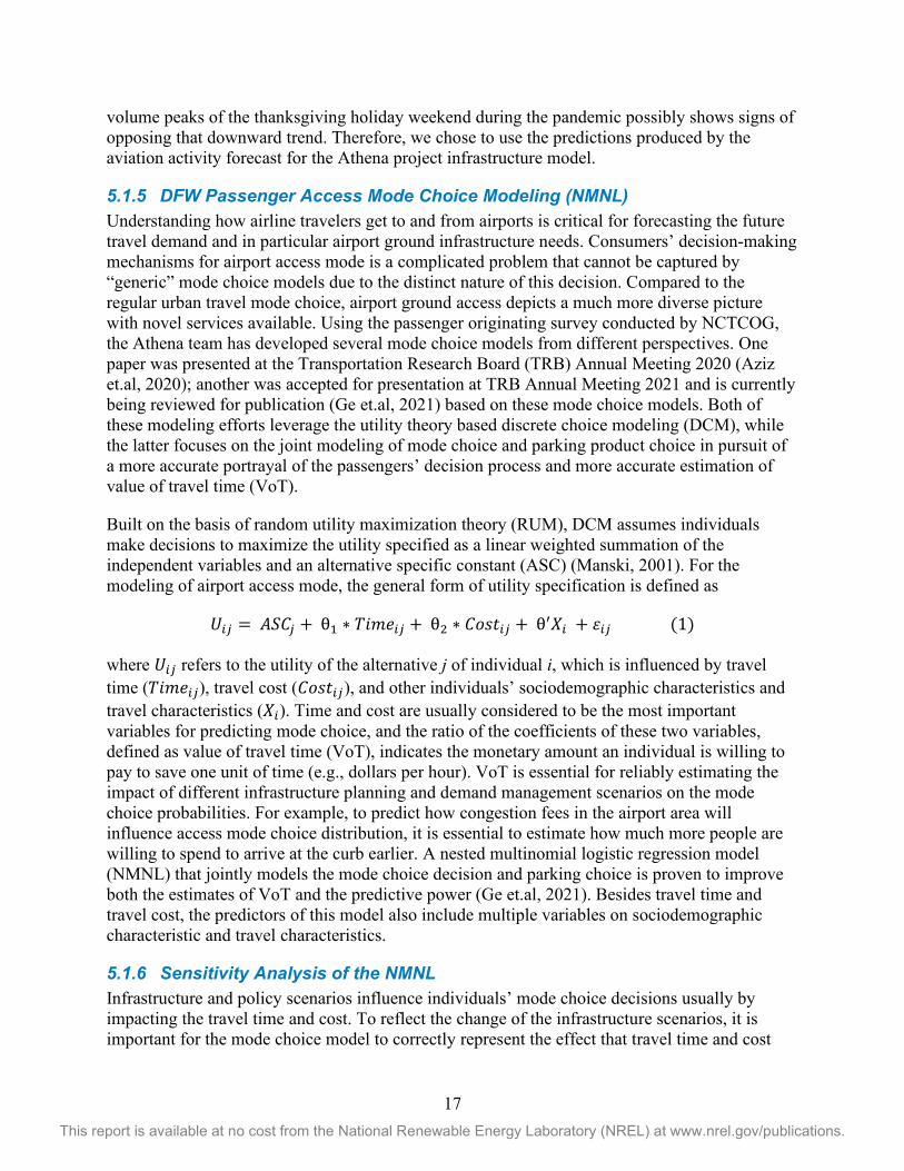
have on individuals’ decisions. To demonstrate this capability of the model we developed, we hereby present an illustrative example with a fictitious individual named Jane who is a middle-aged Dallas-Fort Worth resident, stays 5 miles away from the airport, and has an upcoming leisure trip. Plugging Jane’s individual and trip characteristics in the model, we see that Jane has a higher probability of being dropped off or parking at the airport. If parking, Jane’s top preferences are either to park remotely or at the terminal. We then consider a set of scenarios where congestion fee is introduced in the DFW region and is increased up to a maximum of $80. The congestion fee is reflected in the travel cost for various modes, particularly the car modes. It can be observed from Figure 13 that with increasing congestion fee, Jane’s likelihood of getting dropped off or driving herself (e.g., parking) gradually decrease whereas her likelihood of taking transit increases exponentially. Even in parking choices, with increased congestion fee, Jane’s likelihood of choosing remote parking increases with increasing congestion fee, consistent with intuition (Figure 13).
(a) Mode choice (b) Parking choice
Figure 13. The mode choice and parking choice probability for Jane with the introduction of congestion fee in DFW area. (The solid lines represent the estimates of the probabilities and the
shaded area represents the 95% confidence interval.)

19 This report is available at no cost from the National Renewable Energy Laboratory (NREL) at www.nrel.gov/publications.
(a) Mode choice (b) Parking choice
Figure 14 The mode choice and parking choice probability for Jane when terminal parking price changes. (The solid lines represent the estimates of the probabilities, and the shaded area
represents the 95% confidence interval.)
Similarly, when terminal parking prices are increased, Jane’s likelihood of parking decreases whereas her likelihood of getting dropped off or taking a TNC improve. Unsurprisingly, with increase in cost of terminal parking, Jane’s likelihood of parking at the terminal decreases exponentially, coupled with a complementary increase in remote parking.
5.1.7 Enhancement of NMNL Based on Future TNC Mode Share (NMNL+) As the NCTCOG survey was conducted during late 2015 and early 2016, the share structure looks different from the current, especially for Transportation Network Companies (TNC) which work in a young service. The NCTCOG survey shows that the mode share of TNC was a little over 5%, while a more recent survey conducted in 2018 by a DFW team showed TNC mode share reached about 23%. To facilitate infrastructure planning for future years, one important question to answer is whether TNC services had reached the peak of their market penetration in 2018 to 23%. By combining the plaza data and the transaction data of different services, we estimated the monthly mode share for the airline passengers’ access trips from October 2013 to January 2020, as shown in Figure 15. Using a Bass Diffusion Model, we projected the adoption of TNC in the future years and learned that the peak of TNC mode share is about 25% if both the industry and the airport infrastructure/policy stay the same (Figure 16).

20 This report is available at no cost from the National Renewable Energy Laboratory (NREL) at www.nrel.gov/publications.
Figure 15: DFW Airport Mode Share
Figure 16: TNC Adoption Projection Using Bass Diffusion Model
Instead of applying the NMNL model directly to the synthetic passenger data described by Section 5.1.6 for the prediction of mode and parking choice, another step is carried out to augment the model to better represent future mode share structure which generates the augmented model NMNL+. The alternative specific constants (ACSs) were arbitrarily adjusted to arrive at a more realistic mode share for TNC, a practice that is quite common among agencies due to the difficulty of updating survey data frequently (Kisia, 2017).
5.1.8 DFW Passenger Egress Mode Choice While a lot of effort is spent on developing a suitable mode choice model for the passengers’ access trips, egress trip mode choice gets limited attention due to the lack of data, a conundrum that is shared by other researchers (Gupta, 2008) and agencies (Gosling, 2008). The only piece of literature that looks at the egress mode choice model is by Reibach (2013), who estimated both access and egress mode choice models for a few airports in California using a survey conducted by Metropolitan Transportation Commission (MTC) in 2001-2002. Considering the regional

21 This report is available at no cost from the National Renewable Energy Laboratory (NREL) at www.nrel.gov/publications.
differences and the changes that have happened in transportation in the past two decades, the detailed egress mode choice models developed by Reibach do not bear enough value to be directly applied in the case of today’s DFW airport. However, the relationship between the access and egress trips illustrated in the paper shows a possible path to circumvent a detailed egress model, which is valuable when a rigorous modeling process is prevented by the lack of data. Ultimately, Reibach (2013) shows that the access mode is a predictor of egress trip, for example when some parked their car at the airport for a departure flight, the corresponding arrival flight trip will have egress mode of driving the parked car. Based on the access/egress mode share relationship listed in that article, we constructed the egress mode share for any given access mode for each market segment and the results for residents on business trips are shown by Table 3. A few assumptions were made, particularly surrounding the newly emerged mode TNC which was not in the picture when the MTC data was collected in 2002. When the access mode is drop off or transit for a Texas resident that is on a business trip, it is assumed that some of the percentage of taxi egress will be diverted to TNC due to cost considerations. When TNC is chosen as an access mode, in most cases, TNC will be chosen as the egress mode as well. Admittedly, though the research by Reibach offers some basis for those choices, these numbers are still chosen arbitrarily and should be replaced once more accurate data is available. For the synthetic tickets for arriving passengers, an access mode is first assigned based on the access mode choice model NMNL+, and then the egress mode is assigned based on this relationship between access and egress mode.
Table 3: Relationship Between Access and Egress Mode Share (Approximated)
Texas residents on business trips
Egress mode
Picked up
Parked Car TNC Taxi Airport
shuttle Transit
Access Mode
Dropped off 76% 0% 11% 8% 2% 3%
Parking 0% 100% 0% 0% 0% 0%
TNC 16% 0% 81% 0% 1% 2%
Taxi 16% 0% 0% 81% 1% 2%
Airport shuttle 30% 0% 0% 0% 70% 0%
Transit 18% 0% 11% 0% 0% 71%
5.1.9 Using NREL High-Performance Computer (HPC) Eagle for Mode Choice Datasets Generation
The processes listed in Figure 7, from synthetic tickets, to generating synthetic passengers, to leveraging model choice models, to the final product of passenger volume data for each mode, are run for multiple iterations to cover the variations due to time of the day, day of the week, month of the year, and different infrastructure pricing scenarios. For each of these scenarios, multiple repetitions (10+) are generated to reflect the uncertainty of mode choice decisions for one given set of passengers in one specific infrastructure scenario. As a result, hundreds of thousands of runs within the same procedure are required. NREL’s HPC system, Eagle, facilitates the parallel computing of these runs. In Eagle, the parallel jobs are structured to take advantage of all the 32 cores of each node.

22 This report is available at no cost from the National Renewable Energy Laboratory (NREL) at www.nrel.gov/publications.
5.2 Athena SUMO model 5.2.1 DFW Terminal Area Modeling To represent the DFW terminal curbside behavior, we built the SUMO microsimulation model from a road network and a demand model comprised of various route trips. For the network, we extracted the DFW airport from OpenStreetMap. The network captures various attributes of the airport geometries. We validated the network by adjusting road speeds to observed speeds from TomTom probe data. For the demand side of the model, we utilized predicted traffic demand forecasts from our previously developed demand predictive model. We developed a terminal-specific driver behavior model to better evaluate the travel time for curbside pick-up/ drop-off (PUDO). The terminal behavior model has two components: 1) a more realistic curbside driving model and 2) a garage-parking-as-remote-curb model.
We developed a native SUMO function to simulate the PUDO behavior at the curbside and to set stops at the curb links. Using this function, the vehicles will queue one after another on the right most lane. When the early-arrival vehicles finished PUDO and open the downstream curbside, the newly arrived the vehicles will still queue after the last vehicle. In reality, the human drivers behave differently:
1. the vehicles stop at a random location along the curbside instead of following a queue; 2. the later arrived vehicles could go to the front and use the recently opened curb space;
and 3. when the right most lane (curbside) becomes fully occupied, the newly arrived vehicles
may stop on the second right most lane (double parking). We developed a more realistic curbside driving model to achieve the aforementioned human driver behaviors. As shown in Figure 17, the curbsides are divided into a number of parking spaces (shown in blue color). The PUDO vehicles (the red passenger cars) will stop randomly on the open parking spaces for a PUDO duration following a uniform distribution. If the curbside parking spaces are all occupied, the driver will pick a random location to wait. As the vehicle slows down, if there is a new parking space open down the road, the driver will move on to the newly opened parking space. If there is still no open space after the vehicle is fully stopped, the vehicle will use the stop (on the second lane or the third lane) to pick up or drop off passengers. The vehicle will park where it is stopped and stop for a random PUDO duration.

23 This report is available at no cost from the National Renewable Energy Laboratory (NREL) at www.nrel.gov/publications.
Figure 17: DFW Curbside Terminals

24 This report is available at no cost from the National Renewable Energy Laboratory (NREL) at www.nrel.gov/publications.
Figure 18: Curbside parking at an airport terminal
In Figure 19, we compared the behavior of SUMO driver models (in red) to our custom driver behavior algorithm (in dashed blue). The x-axis is the demand generated as an input to the simulation and the y-axis is the observed output flow over the PUDO edge during the simulation. We can tell from the figure that the custom algorithm increased the capacity of the curbside by implementing a more realistic behavior of drivers. This is shown by an average increase in observed flow in vehicles per hour over the curbside edge compared to the default driving behavior.
Figure 19: Comparing SUMO default driving behavior to realistic curbside driving model.

25 This report is available at no cost from the National Renewable Energy Laboratory (NREL) at www.nrel.gov/publications.
The garage-parking-as-remote-curbs model is a queuing model which takes the overflow of curbside traffic to the garage at the terminal and uses part of the garage as PUDO zones. The newly arrived vehicle chooses to go to parking garage at the terminal if the curbside parking spaces are fully occupied. When a vehicle goes to the parking garage, it is removed from the road network in the SUMO simulation and is added to a virtual queuing system to model the garage parking pick up and drop off process. Within the parking garage, we define a certain number of parking spots converted as “remote” curbside spaces. Vehicles going to a parking garage for PUDO will use the parking spaces. After PUDO, the vehicles will be added back to the road network to leave the terminals.
5.2.2 Remote Curbside Modeling Another part of our SUMO modeling deals with simulating remote curbside areas at the north remote parking and south remote areas at DFW as shown in Figure 20. These remote curbs would be used by DFW patrons to either avoid congestion within the DFW terminal areas, or to avoid having to pay a fee to access the terminal curb spaces. Figure 21 shows the base network for this remote curb simulation. We used a simple geometry with straight lines to limit the complexity of network modifications for curbside expansion. In the diagram, the top road segment, shown as ‘Remote Pickup Drop off Curbside,’ represents where the passengers are to be dropped off or picked up. The lower road segment represents where the airport shuttles would collect the passengers for transport to their respective terminal for departing flights. Arriving passengers who are being collected at the terminal are also dropped off at the ‘Remote Bus PUDO Curbside’ to leave the airport. In the middle, between the two road segments, is the pedestrian median where patrons can safely walk across to catch a shuttle bus to the terminal or to be picked up at the curbside after being transported by the shuttle.
Figure 20: DFW airport network with North and South Remote Curbside candidates.

26 This report is available at no cost from the National Renewable Energy Laboratory (NREL) at www.nrel.gov/publications.
The incoming lanes refer to the tributary edge feeding the curbside PUDO zone. The incoming lanes are important because they limit the number of vehicles that can pass along the curbside. The remote curbside area is comprised of blue spaces. These spaces are primarily only used on the right-most lane. When the right-most lane slots fill to capacity, double parking occurs, and the middle lane begins to be utilized due to congestion along the right-most lane.
Figure 21: Remote Curb Base Network
We conducted initial analysis where we varied the number of lanes, incoming demand, and number of curbside slots. We found that varying the number of lanes tended to be inconsequential to the outcome of the simulations. This is due to the capacity limitations determined by the number curbside slots. Since on average, the vehicles would stop along the curbside with a dwell time of 90 seconds, we could translate that to the average vehicles per hour that could be serviced within that hour. Subsequently, the number of vehicles serviced per hour could be considered as the capacity along the curbside. Thus, we chose to only explore variation in demand and network length while keeping the number of lanes constant (i.e., two incoming lanes). Looking at Table 4, we can see that two lanes produced a capacity of up to 3,160 vehicles and resulted in a reasonable curbside length of 0.5 miles. As the number of lanes increases, the length of the remote curb also needed to be augmented to accommodate high vehicle flow. At some point, this resulted in a curbside that was unreasonably long (e.g., a remote curb of 3 miles and 6 lanes). Since such long curbside areas would not fit in the two candidate locations identified for building remote curb at DFW, we did not consider them for simulation.
Table 4: Capacity of network given number of lanes and curb spots
Lanes 1 2 3 4
Capacity (vph) 1580 3160 4740 6320
Curbs Required to satisfy Capacity 40 79 119 158
Length in Miles (miles) 0.25 0.5 0.75 0.99
To understand the dynamics, including vehicle travel time and delay, along the remote curbside, we explored various combinations of demand and number of curbs. We analyzed how vehicle delay was influenced by various levels of incoming demand. Once the remote curbside simulation reaches the network capacity, the driving behavior of the vehicles began to breakdown and the simulation produced unrealistic results. Hence, we ignored simulation scenarios with incoming volume greater than the capacity levels. In Table 5, we can see the

27 This report is available at no cost from the National Renewable Energy Laboratory (NREL) at www.nrel.gov/publications.
various ranges of network size and demand generated. Along with each combination of demand and network length, we ran many simulation scenarios with varying simulation seed values and aggregated the resulting performance measures to smooth out the randomness inherent in SUMO simulations. We decided to stop at 80 curb spots and 2 lanes, because we found this was a curbside with a reasonable length of 0.5 miles, given the limited space for building remote curb areas as shown in Figure 9. Additionally, we assumed that if the airport needed more remote curb space, they would build parallel curb areas with 2 lanes and 80 curb spots.
Table 5: Range of demand and curbside slots explored in simulation for remote curb.
Lower bound Upper bound (capacity)
Interval
Demand (vehicles per hour) 100 3200 100
Network curb slots 10 80 10
Curb Length (Feet) 361 2657 328
Free flow travel time in seconds 108 212 N/A
Observed Delay in Seconds [0, 138] [0,537] N/A
In Figure 22, we explore the relationship of incoming demand (flow rate) to the observed vehicle delay given a number of curb spots. Delay is measured as observed travel time over the PUDO edge in the simulation minus the free flow travel time on that same edge. The free flow travel time is estimated by taking the speed limit on the PUDO edge and calculating the time it would take to travel through the edge given a of number curb spots and speed limit of 15 miles per hour plus the average dwell time (90 seconds) on the curb for pick up and drop off.
The orange lines in Figure 22 represents the average delay for each incoming flow rate given a quantity of curb spots (stated in legends). The faint green dots that span vertically for each flow rate represent the individual points of delay for 50 simulation scenarios we ran for each combination of flow and number of curb spots. These are displayed to show the distribution of delay for each scenario. As you can see from the plots, the delay tends to increase until a certain threshold and then begins to plateau. The plateauing occurs at a capacity level dictated by the constraints in the simulation. In real world circumstance, this scenario may look different than this plateauing effect seen in the simulation. For modeling purposes, the point at which the plot begins to plateau is viewed as the point where the remote curb starts to experience severe congestion and is no longer functioning. Thus, in the infrastructure model, these curves are extended using the information prior to the plateau point.

28 This report is available at no cost from the National Renewable Energy Laboratory (NREL) at www.nrel.gov/publications.
Figure 22. Delay due to increased flow, broken down by number of curb spots.
5.3 Shuttle Bus Route Optimization Model The shuttle bus optimization model developed for the Athena project is described in detail in (Sigler 2021). This model is formulated as a mixed integer linear program where the user can specify the number of routes, capacity of the buses, allowable headways, and maximum in-vehicle travel time parameters. The model was developed to optimize shuttle operations that move DFW passengers between the rental car center and the five terminals, which can more generally be thought of as the ‘travel within the airport premises’ problem. The solutions generated by the model consists of a set of routes, each with a specified number of buses and the capacity of the bus servicing it. The optimization model was designed with some concepts from the classical VRP with pick-up and delivery time windows but was augmented and modified in

29 This report is available at no cost from the National Renewable Energy Laboratory (NREL) at www.nrel.gov/publications.
many ways to accomplish the goals associated with the ‘travel within the airport premises’ problem. In order to conduct meaningful optimization runs with respect to the DFW rental car center, DFW provided access to their vehicles and data systems. DFW allowed NREL researchers to collect Controller Area Network (CAN) bus data from the airport rental car shuttles using vehicle data loggers resulting in approximately 100,000 miles of 1Hz data from 14 buses over a period of one month of shuttle operations (Kotz, 2020). DFW also provided Spatial Positioning on Transit (SPOT) data, which uses commercial hardware to capture information pertaining to shuttle operations. SPOT data combined with CAN data provided the information required for the optimization model.
Moving passengers between a remote curb and the five DFW terminals is another ‘travel within the airport premises’ problem where the insights gained from the rental car center route optimization work was relevant. One key insight from the optimization work conducted with respect to the DFW rental car center was data driven assignment of shuttles, by time of week, using the standard buses on the standard routes was an easy to implement solution that could save up to 20% in energy consumption but only increase the average passenger wait time by 2 minutes. An example of some results which exhibit these features in shown in Figure 23. Since it is likely the DFW remote curbs, if implemented, would have similar travel times to remote curb, given the layout of the current airport, we used these insights and implemented the remote curb busing system in our infrastructure model such that the standard buses and routes were used but the number of buses in service is determined in a data driven fashion by time of week.
Figure 23: Optimal routes computing assuming 43 passenger buses, a 20 minute headway, a 15
minute max in vehicle travel time, and a passenger arrival rate two standard deviations above the empirical mean arrival rate.
5.4 Athena ASPIRES model In order to model and conduct detailed evaluations of operations at an airport bus system, an event driven simulation was developed named ASPIRES (Airport Shuttle Planning and Improved Routing Event-driven Simulation). This simulation was originally motivated by the need to test the routes computed by the route optimization model for the DFW rental car center. Thus, a digital twin of the DFW rental car center was constructed and was engineered within framework general enough to test other shuttle systems.

30 This report is available at no cost from the National Renewable Energy Laboratory (NREL) at www.nrel.gov/publications.
This simulation model was developed as a Python module using SimPy to simulate and evaluate current and potentially improved future airport shuttle operations (Matloff, 2008). The simulation model tries to address the hard-to-calibrate problems faced by most traffic simulation packages and is mainly driven by empirical distributions of real-world data which drive the simulation rather than a calibration process. The more data collected, the more realistically the simulation can perform. The simulation has been highly optimized for runtime speed, as a result simulating one day of shuttle operations takes around one second. The ability to execute fast simulations enables the exploration of many different infrastructure configurations and operational policies under a wide range of different scenarios.
The simulation model can simulate travel times, dwell times, and passenger arrivals using empirical distributions to capture the stochastic nature of DFW’s rental car center shuttle bus operations. Outputs show passenger statistics, shuttle statistics, and charging station statistics for EV buses. The passenger statistics include the waiting time of each passenger, the queue length of each stop at any time, the number passengers left after each shuttle bus pickup, and the total travel time from one stop to another stop. The shuttle statistics include the routes record, the number of passengers onboard at any time, the distance traveled until any time, the energy consumed until any time, and the location of each bus at any time. The charging station statistics record, at any time of the day, the number of chargers being used.
Using the simulation model and the shuttle operation data, we can simulate and evaluate different system designs of a shuttle bus system. Figure 24 shows a sample state of charge (SoC) profile of an electric bus during a week of simulation. Figure 25 shows the charger usage profiles for 28 days of a simulation and for an initial warm up day.
Figure 24: Sample SoC profile of an electric bus for one week.

31 This report is available at no cost from the National Renewable Energy Laboratory (NREL) at www.nrel.gov/publications.
Figure 25: Charger usage profile. On the left is the profile for a 29-day simulation where the first
day is a warm-up day. On the right is the charger profile for the warm-up day.
Using these features a simulation-based optimization model was developed to address the charging station planning problem for an electrified bus system. The studied shuttle system connects the rental car center and the five terminals at DFW and has a fleet of 46 compressed natural gas (CNG) buses. During operation, only 29 buses are needed to ensure the maximum service frequency. The ratio between the fleet size and the number of activate buses is about 46/29≈1.6. Using the simulation-based optimization model and a genetic algorithm, we found that to replace all CNG buses with battery electric buses while minimizing the total capital cost and maintaining the current service frequency, we need to equip electric buses with a battery capacity of 50 kWh and install 4 chargers with a charging power of 210 kW. However, after conversations with DFW, it was determined that the logistical challenges of having small batteries that charge quickly but often would be unrealistic although our optimization showed it was the most cost-effective option. Instead, DFW recommended we use 550kWh batteries and chargers with 90 kW charging speed in our modeling. These recommendations were based on conversations DFW has had with different EV bus vendors.
To inform the needed model parameters in our infrastructure model for the remote curb bus system, we assume that remote curb shuttle systems will have similar locations and characteristics as the rental car shuttle system. Therefore, we assume that the battery capacity of electric buses will be 550 kWh and the charging power of chargers will be 90 kW. Based on simulations conducted, it was determined that 8 chargers would be needed to electrify the rental car center bus fleet and the current level of service. This implies that the ratio between the fleet size and the number of chargers should be 46/8=5.75 at the remote curbs. The ratio of active buses to total fleet size was chosen to be 46/29≈1.6 in accordance with the rental car fleet. Using these statistics from simulations, we were able to construct the needed constraints in the infrastructure model accurately determine the needed number of buses and chargers for different sizes of remote curbs.

32 This report is available at no cost from the National Renewable Energy Laboratory (NREL) at www.nrel.gov/publications.
6 Results 6.1 Model Implementation and Solution Process Alongside those supporting models discussed in the previous section, we have implemented the core optimization model discussed in Appendix A using the open-source algebraic modeling language Pyomo, and we have leveraged the mpi-sppy python package which works in conjunction with Pyomo. Mpi-sppy provides an HPC ready scalable framework for constructing and solving multi-stage-stochastic programs. Our results have been obtained using the mpi-sppy implementation of progressive hedging on the NREL HPC system, Eagle, using 144 nodes and 4,320 cores. Each of our model runs problem considers 21 years of operations and 90 TSAROs for each year leading us to consider 90*21*16= 30,240 operational circumstances. The full undecomposed problem is a mixed integer linear programming problem that has approximately 200 million decision variables. To solve the problem, we decompose it into 1440 subproblem which progressive hedging solves in parallel to get a solution to the global model. The results from running progressive hedging on our problem indicate that the solutions obtained are within 1.4% [SD1] if the optimal solution, and we are usually able to compute solutions in less than 30 minutes of wall clock time [SD1].
6.2 Parking Conversion to Curb Space In order to understand the benefits of converting parking spaces in the terminal parking lots to passenger PUDO spaces, a large number of SUMO simulations were run with different percentages of cars visiting terminal parking lots instead of the curb. These experiments were done to construct surrogate functions that would characterize, for a fixed volume of cars visiting a terminal curb, the degree congestion in the terminal area would be reduced by converting different numbers of parking spots to passenger PUDO spaces. The SUMO experiments revealed that this was not a beneficial strategy for the following reasons:
1. The congestion in the terminal area road network often occurs within on/off ramps (as shown in Figure 26) or due to the weaving of traffic flows (as show in the red circle in Figure 27) and is not due to overcrowding of the terminal curb areas.
2. The parking garages are not designed to handle high throughput of cars, and ramps associated with the garages can get crowded because of this.

33 This report is available at no cost from the National Renewable Energy Laboratory (NREL) at www.nrel.gov/publications.
Figure 26: DFW road network with cars backing up on the ramp to enter a terminal curb area.
Figure 27: Weaving of Traffic Flows
Thus, we often saw in our SUMO experiments that routing cars through the terminal garages made congestion worse. Based on these experiments, it seems that road infrastructure based on easing difficult lane changing for drivers and expansion of congested on/off ramps would be a more favorable approach for reducing terminal area congestion. These road network augmentations were out of scope for the Athena project but could be an interesting topic of research in the future.
As a result of these observations, we eliminated the parking conversion form of infrastructure expansion from our model runs and only considered building remote parking and remote curb infrastructure. This elimination led the model to address terminal area congestion by reducing the number of cars that enter the terminal area at all. This is achieved the using congestion pricing and building lower cost options outside of the terminal area (i.e., remote curb, and remote parking).

34 This report is available at no cost from the National Renewable Energy Laboratory (NREL) at www.nrel.gov/publications.
6.3 Quasi Dynamic Pricing The infrastructure model chooses prices for different parking products and terminal curb access. For each year, prices are set for 16 different time points (season, day of week, time of day). In our work, season is either {Fall, Winter, Spring, or Summer}. Day of week is either {weekend or weekday}, and time of day is either {on-peak or off-peak}. Hence, there are four times of the week where prices are set, and those prices are set each season of the year. For the purposes of our model, the prices set at those four times of week can be thought of as constant over the season. For example, the Fall weekday on-peak price can be thought of as relatively constant over the Fall season. In practice, these prices could be set at the monthly, weekly, or daily level. It is possible that they could even be set in real time. However, DFW has shared that their market research indicates that passengers want transparency into the prices they will pay at the airport at the time they plan their trip. Hence, at this point in our research we are only making the leap from static prices to quasi dynamic pricing, where there are prices set for different times of the week which vary seasonally. We think this strikes the right balance between a novel pricing approach, customer transparency, and practicality.
Another aspect of pricing is the rate at which we allow the prices to increase from their current levels and under what conditions we allow the prices to increase. Since having the remote curb provides passengers with a free option, it seems reasonable to allow prices to be increased once it is built. However, even once the remote curb is built, it does not seem reasonable to let the prices be raised too quickly. Thus, to have a more realistic implementation of prices, we allow the upper boundary for the prices to be raised one increment each year until a maximum price level is hit. The increments are either $5 for remote parking and terminal congestion or $8 for terminal parking. Valet and express parking are raised proportionally to terminal parking. Below in Figure 28, one can see how the upper bounds on prices would increase if a remote curb was built in 2030.
Figure 28: Plot of toll upper bounds over time if remote curb was built in year 2030.

35 This report is available at no cost from the National Renewable Energy Laboratory (NREL) at www.nrel.gov/publications.
In the case that remote curb is not built, we specify that the model must keep the prices at their current levels. This is to ensure that the model does not allow the airport to exert unrealistic monopoly behavior on its customers. The current mode choice model is not equipped to represent passengers choosing other airports, other forms of travel, or deciding not to travel at all. These effects would be relevant if the model was able to charge high prices without providing an affordable option like the remote curb. Therefore, for the results reported the prices are not raised if remote curb is not built.
6.4 Passenger Experience To ensure the model makes infrastructure decisions which account for the DFW passenger customer experience, customer service penalties are included in the model. As depicted in Figure 5 in Section 4, these customer service penalties are related to parking, the busing of passengers to and from terminals, and congestion at remote curbs and the terminal area. In particular, for parking the customer experience penalties are as follows:
• If a parking lot overflows it is assumed those people go to another parking lot to park. It is assumed this takes them 15 minutes to move to the other parking. As a result, the model’s objective function in penalized (0.25 hours) * (an hour of a DFW passengers’ time) for each person this happens to.
• If all parking at DFW is full, the objective function is penalized the cost of an average DFW flight for each person who cannot park.
In the case of shuttling passengers between terminals, remote curbs and parking lots the customer experience penalties are as follows:
• If a bus leaves a person behind (at parking or the remote curb), it is assumed this delays the customer 15 minutes, and the model’s objective function in penalized (0.25 hours) * (an hour of a DFW passengers’ time).
Finally, in the case of delay at remote and terminal curbs, the customer experience penalties are as follows:
• If the average delay in the terminal area or a remote curb exceeds 10 minutes, it is assumed that the whole airport system begins to slow down, and all passengers are delayed in some manner. This assumption is meant to capture the fact that the airport is a collection of subsystems that influences one another, and failures of performance are not confined to individual subsystems.
• To estimate this effect, we multiply the number of minutes beyond the allowed 10 minute delay by the whole DFW passenger population that hour, and multiple that by the value of time. For example, consider the case where 4,500 people are entering or leaving the airport that hour and the delay at the remote curb is 15 minutes. In this case, we penalize the objective function by the amount 4500*5*(average passengers’ value of time).
We also note that our model uses mode choice behavior that assumes passenger behave under the assumption there is enough capacity in the system for their mode of choice. That is to say, the model does not have any mechanism to capture passengers learning to avoid the remote curb on weekdays at 5:00pm, for example. In the model, the passengers assume a smooth experience when making their mode choice. As a result, our model fails to capture the passenger mode

36 This report is available at no cost from the National Renewable Energy Laboratory (NREL) at www.nrel.gov/publications.
choice patterns that would emerge as a result of previous experiences had by passengers. Finally, in our model, passengers do not have the option of not flying or choosing a different airport. In reality, large delays or high prices might cause passengers to exercise these options. Future work could include enhancing the model to account for these more complex mode choice dynamics so stress on the system could more accurately be captured through the penalties mentioned above.
6.5 Simulation of Infrastructure The infrastructure model uses a two-stage model to compute optimized infrastructure modifications to the airport. However, there are different levels of uncertainty present in actual airport operations which could justify a three or even four stage stochastic model. For example, infrastructure must operate well under a variety of operational circumstances, and the infrastructure decisions must be made years or even decades before those circumstance might arise. This alone necessitates a two-stage model where the first stage decisions are infrastructure improvements, and the second stage decisions are daily operations decisions for different airport circumstances that might arise in the future. Yet, daily operations’ decisions must be made under uncertainty as well. For a current example, consider that mode choices and demands on the system are stochastic, and making decisions about how many buses to use on different “within premises airport shuttle routes” must be made under uncertainty. Another example relevant to the infrastructure model in this report is congestion pricing effects on mode choices. When the prices are set ahead of time, it is not known precisely how the population of passengers will respond to the prices and how mode choice volumes will materialize as a result. Such operational uncertainties can be represented with a third stage in the model, where a single set of prices are chosen for a set of possible mode choice responses from the DFW passengers. Unfortunately, trying to solve such versions of the model has proved intractable at this stage in our research. Thus, we have used a two-stage model as an approximation of a three-stage model. This comes at the risk of our model underestimating the infrastructure needed for efficient airport operations. The reason for this is that our two-stage infrastructure model assumes that operational decisions are made with certain information and perfect forecasts regarding demand and mode choice behavior. The need for the third stage in the infrastructure is largely dependent on how well demand and mode choices responses to prices can be forecasted. An additional factor is how dynamic of a pricing scheme DFW customers will tolerate. If high quality forecasts can be created and used in conjunction with a pricing scheme that is sufficiently dynamic, the need for a three-stage model is reduced.

37 This report is available at no cost from the National Renewable Energy Laboratory (NREL) at www.nrel.gov/publications.
Figure 29: DFW infrastructure simulation workflow.
To test the performance of the optimized infrastructure computed using the two-stage model, we developed a simulation workflow to evaluate the infrastructure decisions under more realistic operations conditions. The workflow proceeds as follows: First, operational models are constructed for a variety of future hours with the prescribed infrastructure and a forecast of demand and mode choice behavior. These models are then solved, and the pricing decisions computed are extracted. Next, a second set of operational models are constructed for the same hours using the prescribed infrastructure, the actual demand, and mode choice behavior, and the computed prices as fixed parameters. These models are then solved, and various performance information is saved and aggerated to access the quality of the infrastructure decisions. This process allows us to explore how the quality of the operational forecast used to set prices affects operational performance. We show in the later sections of this report that the effect can be significant and further research into how to solve three stage versions of this model could be warranted.
The actual demand and mode choice behavior is represented by 9 additional TSAROs for each year. If mode choices responses to prices can be perfectly forecasted, the two operations models will use these 9 additional TSAROs for each year. If we consider imperfect forecasts, then the first operational model for determining prices will use randomly chosen TSAROs as the forecast of demand and mode choice behavior.
6.6 Standard Model Results The standard model represents a baseline version of the model that has the best estimates that could be made for the model parameters and does not consider AVs. The model determines infrastructure to be built while considering its cost, the cost of bus and remote curb operations, emissions costs, and customer service penalties which are translated to people value of time and costs of missed flights. Here we present the infrastructure prescribed by this version of the model.

38 This report is available at no cost from the National Renewable Energy Laboratory (NREL) at www.nrel.gov/publications.
6.6.1 Standard Model Infrastructure Results The primary purpose of this model is to obtain a timeline of infrastructure improvements. These are relatively straight forward to visualize. Figures 30-31 show the infrastructure build results. In these results the model determines the decisions that would maximize revenue, and minimize infrastructure costs, operations costs, emissions costs, and costs the model imposes for poor passenger service. Here, we see that from Figure 30 the remote curb is expanded incrementally every five years at both the “north” and “south” sites along with cell phone parking spots, for vehicle staging purposes. As discussed in the next section, it appears remote curb used in conjunction with dynamic pricing provides a mechanism to manage terminal congestion and generate revenue for the airport. It also seems plausible that it can reduce terminal area emissions by a non-trivial amount.
Figure 30: Plot of remote curb pickup/dropoff spots and vehicle staging parking spots expanding over time for the north and south remote locations.
Figure 31: Plot of remote curb electric bus and charger deployment over time. The plot shows
steady growth in EV bus and charger infrastructure to accommodate increasing remote curb and parking shuttle needs.
In Figure 31, the battery electric buses used to move passengers between the terminals and the remote curb are purchased gradually over the planning horizon as the remote curbs are expanded. The total number of buses fluctuates up and down over time, because the buses are retired after 8 years of service and new buses are only purchased every five years due to the five year investment cycle we assume. This service life of these buses was based on data from DFW’s current bus fleets. This number might be somewhat different with electric buses in practice. In practice, DFW might purchase the buses as needed instead of every 5 years which would make the plots in Figure 31 smoother. However, given the 5-year investment periods the model uses, it buys enough buses to handle the forecasted increase in demand plus the number of buses

39 This report is available at no cost from the National Renewable Energy Laboratory (NREL) at www.nrel.gov/publications.
scheduled to be retired from use in the next 5 years. We also see in Figure 31 on the secondary vertical axis, the number of chargers gradually increasing with the number of buses over time. Remote parking is significantly expanded at the first parking expansion opportunity and then once more to a lesser degree at the last building opportunity in the horizon. There are a few possible reasons for this significant expansion in parking. One reason is that it is a cheaper form of infrastructure relative to remote curb, however, like remote curb, it does require the purchase of buses and chargers. Similar to the remote curb high terminal area, pick-up/ drop-off tolls and parking terminal tolls have the ability to divert people to remote parking, thus it might be an attractive option for reducing terminal congestion assuming dynamic pricing can be used. Another possible reason for the large amount of parking built is a sensitivity in the model parking constraint to the average duration people park and the hourly incoming volume of cars. The average occupancy of parking lot can be estimated by multiplying the average duration parked by the average arrival rate of incoming cars. This fact is used in the models parking constraints which estimate parking lot occupancy. Due to the quadratic nature of this estimate errors in average duration or the volume of cars arriving can lead to drastic overestimations of the occupancy and result in the model overestimating the needed number of parking spots. Such errors could be causing the large number of remote parking spots recommended. Regarding the remote parking buses, similar behavior is observed in Figure 32 as in Figure 31, which shows the number of battery electric buses and needed chargers added over time to the fleet that serves the remote parking lots. We note that the north and south remote parking lots are not served by separate routes, so they share a bus fleet and a set of chargers. Finally, we note our results indicated that for both the “north” and “south” remote curb sites, two car lanes and one bus lane are constructed for access purposes.
Figure 32: Plot of remote parking expansion and the supporting electric bus and charger
deployment over time.
In Table 6, we provide a complete summary of all the infrastructure built in total over the horizon which complements figure 33, where those improvements are visualized along the 25 year timeline. We also provide the sources that were used to estimate the costs of different infrastructure improvements. We note that all costs provided are in 2021 dollars. In total the model recommends $336,105,000 in infrastructure improvements over the 2025 to 2045 horizon. In the following section we provide an analysis of operational simulation results where these infrastructure decisions were tested. This analysis provides deeper insight into why the model recommends these specific infrastructure improvements.

40 This report is available at no cost from the National Renewable Energy Laboratory (NREL) at www.nrel.gov/publications.
Table 6: Recommended infrastructure costs.
Item Quantity Costs Data Source
Total Cost
Remote Curb Space With Rain Shelter
140 $145,000 per spot Industry Experts, (Bushell et al. 2013)
$ 20,300,000
Remote Curb Staging Parking Spaces
109 $5,000 per spot Industry Experts, DFW survey, (Broin et al. 2017)
$545,000
Remote Curb Connecting Road Miles
6 $2,360,000 per mile (Broin et al. 2017)
$14,160,000
EV Buses 550 Kwh Battery) 314 $800,000 per bus DFW $251,200,000
EV chargers (90 Kw) 37 $100,000 per charger DFW $3,700,000
Remote Parking Spaces 9240 $5,000 per spot Industry Experts, DFW survey, (Broin et al. 2017)
$46,200,000

41 This report is available at no cost from the National Renewable Energy Laboratory (NREL) at www.nrel.gov/publications.
Figure 33: Timeline describing recommended infrastructure builds for baseline scenario.
6.6.2 Standard Model Operations Results To estimate how the infrastructure prescribed in Section 6.6.1 would perform, we performed the simulation procedure described in Section 6.5. The actual demand and mode choice behavior was represented by 9 additional TSAROs for each year. This provides in total 3,024 operational time points where the infrastructure is simulated. We conducted the simulations in two ways. The first way assumed the demand and the mode choices responses to prices can be perfectly forecasted. The second way assumes these quantities can be forecasted but in an imperfect manner. In the case, where the mode choices responses to prices can be perfectly forecasted, both the operations model and the operations model with fixed prices use these 9 additional TSAROs for each year. In the case where we consider imperfect forecasts, the operational model for determining prices uses a randomly chosen TSARO from the pool used for the infrastructure model as a forecast of demand and mode choice behavior, and the operations model with fixed prices uses the 9 additional TSAROs for each year as “actuals.” By simulating the performance of the infrastructure in these two ways, we can better understand the impacts of inaccuracies in operational forecasts. It can be informative to visualize operational decisions from the simulation to understand how the model is operating the airport and utilizing the infrastructure built within the simulation. The results presented in this section are for the case where forecasts are perfect unless otherwise specified.

42 This report is available at no cost from the National Renewable Energy Laboratory (NREL) at www.nrel.gov/publications.
To show the internal mechanics of the operations model used for simulation, we extract the results for one operational context over the 21 year horizon representing a peak hour of operations on a weekday in Summer with a high increasing demand rate and a highly efficient emissions technology adoption rate. Figure 34 shows the prices that were set during this hour over the model horizon. We see large variations in the prices across 21 years. There does appear to be a slight upward trend over time, especially in the terminal parking and PUDO tolls. Since the prices determine the passenger mode choice distribution in the model, it is helpful to look at the mode choice distribution over the model horizon.
Figure 34: Plot of terminal tolls and parking prices for one representative scenario. Terminal
parking price and remote parking price stays relatively constant in this scenario while the congestion toll increases steadily over the 20 year period.
Figure 35 shows the passenger volume distributions for this hour amongst different travel modes across the 21 years. For simplicity, we have grouped airport shuttle, charter bus, hotel shuttle, Park N Fly, Parking Spot, and the rental car center into the category of “other modes.”
Figure 35: Plot of passenger mode distributions for one representative scenario.

43 This report is available at no cost from the National Renewable Energy Laboratory (NREL) at www.nrel.gov/publications.
These modes in the “other modes” category all use shuttles or buses to move passenger to and from the terminal curbs and can, in general, be thought of as high occupancy vehicles. We also note that we have included the valet parking volume in the terminal parking category.
In Figure 36, we show the number of buses in service during this hour over the model horizon. We see that the number of buses in service for this hour changes quite a bit from year to year. Each bus fleet has a minimum number of buses that must be in service. From Figure 36, we can see that remote curb and express parking fleets vary in response to demand, while the remote parking seems to always be operating the minimum number of buses. In studying these figures, we observe that although the prices fluctuate over the years, there seems to be general mode distribution trends that are preserved across the years. We see that the remote curb serves a significant portion of passenger volume, as well as the “other modes” category which uses high occupancy vehicles. Terminal parking is the mode choice with the next largest volume and high profitability for the airport. Transit as a mode appears to be the least attractive mode for passengers and accounts for less than 5% of all passenger volumes. Generally, it seems that prices are being set to keep these trends in place. It appears the number of vehicles visiting the terminal is kept low with higher prices. This seems to suggest that the model is trying to avoid congestion in the terminal areas by pushing volume out to the remote curb, while still creating revenue through high congestion prices and price combinations that encourage high amounts of terminal parking. Figure 37 shows an estimate of the cumulative revenue, only on this hour of interest, from parking fees and congestion tolls over the 21-year planning horizon. The total estimated revenue is about $16 billion.
Figure 36: Plot of number of buses in service for one representative scenario.
Moving away from focusing on an individual hour across planning horizon, we now look at quantities across all 3,024 operational contexts considered by the simulation, where each context represents an hour of operations. These data points can be described in terms of their central tendency, spread, or histograms. One question of interest is, given the 3,024 hours of operations simulated, how wide was the range of mode share percentage for each mode? Were there cases where almost everyone takes a TNC or cases where almost everyone parks at the terminals? To

44 This report is available at no cost from the National Renewable Energy Laboratory (NREL) at www.nrel.gov/publications.
give insight into such questions, Figure 38 provides four box and whisker plots of passenger volume distributions among all travel modes for these 3,024 hours of operations. The four box and whisker plots correspond to the four times of week that were considered in the simulation (on-peak/off-peak and weekend/weekday), and each considers 756 hours of operations. For each mode’s boxplot, the left most whisker represents the lowest data point excluding any outliers (0th percentile), the right most whisker represents the largest data point excluding any outliers (100th percentile), the box shows the range from the 25th percentile to the 75th percentile, the orange line within the box shows the 50th percentile value, and the blue “+” shows the outliers. Outliers are defined as data points that are beyond the range of [25𝑡𝑡ℎ percentile − 1.5IQR, 75𝑡𝑡ℎ percentile + 1.5IQR], where IQR = 75𝑡𝑡ℎ percentile − 25𝑡𝑡ℎ percentile. Figure 37 shows the trend of high remote curb utilization, high utilization of “other modes,” relatively high terminal parking, relatively low terminal curb utilization seems to hold across all 3,024 hours considered. Figure 38 does show appreciable variation, and this trend mostly likely does not hold in each individual hour considered. We also note that there does not seem to be an apparent difference between box and whisker plots regarding the for different times of the week.
Figure 37: Accumulative revenue for one representative scenario.

45 This report is available at no cost from the National Renewable Energy Laboratory (NREL) at www.nrel.gov/publications.
Figure 38: Box whisker plot of passenger mode distributions based on all 3,024 operational
contexts across 21 years.

46 This report is available at no cost from the National Renewable Energy Laboratory (NREL) at www.nrel.gov/publications.
To further investigate the operational behavior of the simulation models, we created three sets of histograms using the 3,024 hours of operational results. The first set of histograms shows terminal congestion prices for a passenger pickup or drop off (toll values) in Figure 39, the second set of histograms shows the percentage of passengers using the remote curb in Figure 40, and the third set of histograms shows the percentage of passengers using terminal curbs in Figure 41. Figure 39 shows that across all these hours of operations the congestion price for passenger pickup and drop off in the terminal area is often higher than the current price of $3.
Figure 39: Histogram of congestion prices for a passenger pickup or drop-off (toll values) based
on all 3,024 operational contexts across 21 years.
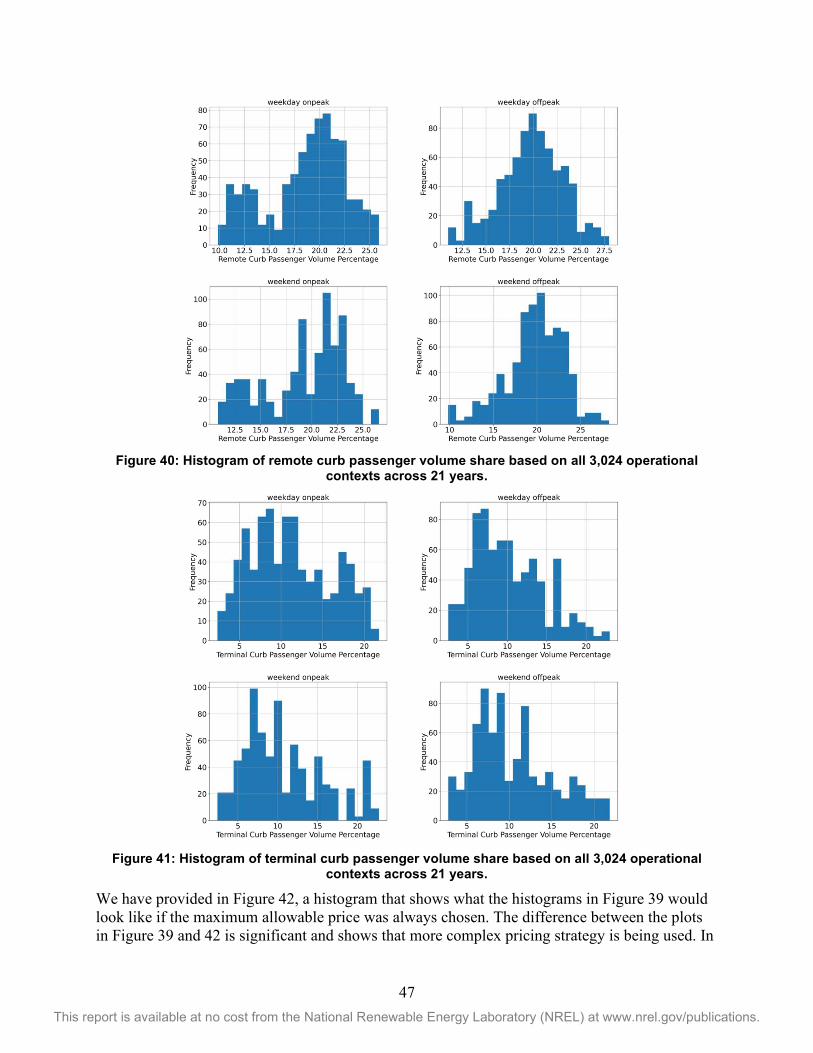
47 This report is available at no cost from the National Renewable Energy Laboratory (NREL) at www.nrel.gov/publications.
Figure 40: Histogram of remote curb passenger volume share based on all 3,024 operational
contexts across 21 years.
Figure 41: Histogram of terminal curb passenger volume share based on all 3,024 operational
contexts across 21 years.
We have provided in Figure 42, a histogram that shows what the histograms in Figure 39 would look like if the maximum allowable price was always chosen. The difference between the plots in Figure 39 and 42 is significant and shows that more complex pricing strategy is being used. In

48 This report is available at no cost from the National Renewable Energy Laboratory (NREL) at www.nrel.gov/publications.
Figure 40, we see that a significant portion of passengers, approximately 12%-25%, are attracted to the remote curb. We note that these histograms seem to be skewed towards 20%, and the on-peak histograms exhibit some bi-modal behavior. Figure 41 shows that approximately 1%-20% of passengers use the terminal curb, and the histograms are skewed towards lower percentages around 10%. Based on these three sets of histograms and that fact that the prices determine the mode choice behavior in our model, it seems reasonable to assume that the higher congestions prices for terminal curb access seem to be driving people away from the terminal curbs. This is likely done to manage terminal congestion and emissions, while generating revenue. This optimization strategy seems to work well with respect to revenue generation. The estimated cumulative revenue across the 21 years is reported in Figure 43 for the high, medium, and low demand growth scenarios. In all three cases revenue is near $12 billion dollars.
Figure 42: A congestion toll distribution assuming the maximum allowed congestion price is used
at each time point. This histogram considers the same 756 points used to make any of the four histograms in Figure 38. This shows that the histograms in Figure 39 show behavior much
different than what is observed if the maximum price always used.
Figure 43: Expected accumulative revenue from parking and terminal toll across 21 years under
different demand scenarios.

49 This report is available at no cost from the National Renewable Energy Laboratory (NREL) at www.nrel.gov/publications.
For completeness we have also visualized the simulation models use of buses over the 3,024 operational scenarios. To understand how the number of buses used varied, we again created four histograms shown in Figure 44. This figure shows the total number of active buses in service for remote parking, remote curb, and express parking. As expected, weekday usually requires more buses than weekend and peak hours require more buses than off-peak hours. The number of active buses for the 3,024 operational contexts ranges from 36 to 65, which further demonstrates the robustness of the bus infrastructure decisions in handling a variety of busing needs.
Figure 44: Histogram of total number of active shuttle buses based on all 3,024 operational
contexts across 21 years.
To demonstrate the value of the recommended infrastructure in context of operations, we constructed a status-quo version of our model that makes no infrastructure improvements and must keep the parking and terminal congestion prices at their current levels. We simulated the system operations under the status quo against the same 3,024 operational hours that we run the infrastructure decisions against. Figure 45 and Table 7 compare the system performance using the optimized infrastructure and the status quo infrastructure. In Figure 45, passenger congestion and overflow costs refer to costs associated with excess delays at the curbs and DFW parking lots being full. Delays at the curb or vehicles needing to go to another parking lot to find open parking spaces are penalized based on the average DFW passengers’ value of time. If parking at DFW is completely full across all lots, each person who cannot park penalizes the operations model the average cost of a DFW flight. One can see that, compared to the status quo with no infrastructure improvements, the recommended infrastructure can significantly reduce the passenger congestion and overflow cost, although it requires some construction cost and operating costs for shuttle and remote curb service. In addition, with increasing upper bounds for parking fees and congestion tolls, the recommended infrastructure leads to much higher expected revenue for the airport.

50 This report is available at no cost from the National Renewable Energy Laboratory (NREL) at www.nrel.gov/publications.
Figure 45: Comparison of lifecycle costs and revenues for optimal solution and status quo.
Table 7: Cost comparison between the airport with recommended infrastructure improvements and status quo infrastructure.
Scenarios Construction Cost ($106)
Total Operating Cost ($106)
Bus and Curb Operating Cost ($106)
Passenger Congestion and Overflow Cost ($106)
Emission Cost ($106)
Revenue ($106)
Optimal Solution 303 1452 612 833 5 12458
Status Quo 0 17247 236 17011 0 7538
Table 8 further compares passenger experience using the optimized infrastructure and the status quo infrastructure. One can see that with the recommended infrastructure, parking overflow probability, especially for terminal parking and remote parking, is significantly reduced compared to the status quo. Particularly, with the recommended infrastructure, the probability of “All Parking Overflow,” i.e., the probability that the total parking demand (including terminal parking, express parking, and remote parking) exceeds the total parking capacity, is reduced from 72.7% in the status quo to 0.6%. For express parking, the overflow probability is only slightly reduced from 37.8% in the status quo to 36.5% in the optimal solution. This observation implies that either the combination of the recommended infrastructure or the dynamic pricing is not able to effectively eliminate the overflow at express parking or the cost (or revenue loss) for distributing the express parking flow to other modes is larger than the overflow penalty.
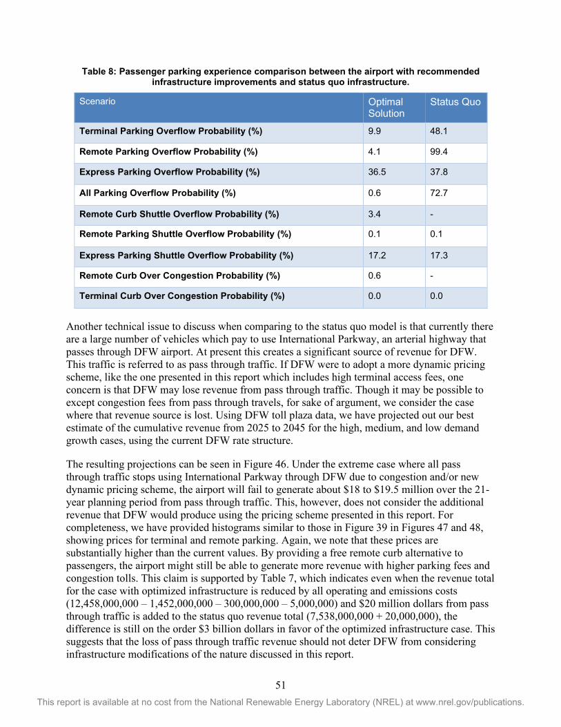
51 This report is available at no cost from the National Renewable Energy Laboratory (NREL) at www.nrel.gov/publications.
Table 8: Passenger parking experience comparison between the airport with recommended infrastructure improvements and status quo infrastructure.
Scenario Optimal Solution
Status Quo
Terminal Parking Overflow Probability (%) 9.9 48.1
Remote Parking Overflow Probability (%) 4.1 99.4
Express Parking Overflow Probability (%) 36.5 37.8
All Parking Overflow Probability (%) 0.6 72.7
Remote Curb Shuttle Overflow Probability (%) 3.4 -
Remote Parking Shuttle Overflow Probability (%) 0.1 0.1
Express Parking Shuttle Overflow Probability (%) 17.2 17.3
Remote Curb Over Congestion Probability (%) 0.6 -
Terminal Curb Over Congestion Probability (%) 0.0 0.0
Another technical issue to discuss when comparing to the status quo model is that currently there are a large number of vehicles which pay to use International Parkway, an arterial highway that passes through DFW airport. At present this creates a significant source of revenue for DFW. This traffic is referred to as pass through traffic. If DFW were to adopt a more dynamic pricing scheme, like the one presented in this report which includes high terminal access fees, one concern is that DFW may lose revenue from pass through traffic. Though it may be possible to except congestion fees from pass through travels, for sake of argument, we consider the case where that revenue source is lost. Using DFW toll plaza data, we have projected out our best estimate of the cumulative revenue from 2025 to 2045 for the high, medium, and low demand growth cases, using the current DFW rate structure.
The resulting projections can be seen in Figure 46. Under the extreme case where all pass through traffic stops using International Parkway through DFW due to congestion and/or new dynamic pricing scheme, the airport will fail to generate about $18 to $19.5 million over the 21-year planning period from pass through traffic. This, however, does not consider the additional revenue that DFW would produce using the pricing scheme presented in this report. For completeness, we have provided histograms similar to those in Figure 39 in Figures 47 and 48, showing prices for terminal and remote parking. Again, we note that these prices are substantially higher than the current values. By providing a free remote curb alternative to passengers, the airport might still be able to generate more revenue with higher parking fees and congestion tolls. This claim is supported by Table 7, which indicates even when the revenue total for the case with optimized infrastructure is reduced by all operating and emissions costs (12,458,000,000 – 1,452,000,000 – 300,000,000 – 5,000,000) and $20 million dollars from pass through traffic is added to the status quo revenue total (7,538,000,000 + 20,000,000), the difference is still on the order $3 billion dollars in favor of the optimized infrastructure case. This suggests that the loss of pass through traffic revenue should not deter DFW from considering infrastructure modifications of the nature discussed in this report.

52 This report is available at no cost from the National Renewable Energy Laboratory (NREL) at www.nrel.gov/publications.
Figure 46: Expected accumulative revenue from passing-through traffic across 21 years under
different demand scenarios.
Figure 47: Histogram of terminal parking fees based on all 3,024 operational contexts across 21
years.
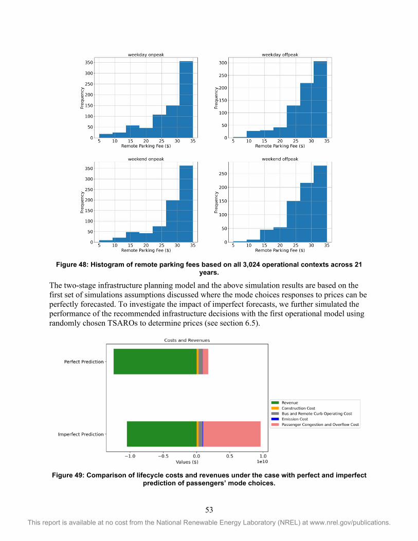
53 This report is available at no cost from the National Renewable Energy Laboratory (NREL) at www.nrel.gov/publications.
Figure 48: Histogram of remote parking fees based on all 3,024 operational contexts across 21
years.
The two-stage infrastructure planning model and the above simulation results are based on the first set of simulations assumptions discussed where the mode choices responses to prices can be perfectly forecasted. To investigate the impact of imperfect forecasts, we further simulated the performance of the recommended infrastructure decisions with the first operational model using randomly chosen TSAROs to determine prices (see section 6.5).
Figure 49: Comparison of lifecycle costs and revenues under the case with perfect and imperfect
prediction of passengers’ mode choices.

54 This report is available at no cost from the National Renewable Energy Laboratory (NREL) at www.nrel.gov/publications.
Figure 49 compares the system performance with perfect and imperfect forecasts. One can see that compared to perfect forecasts, imperfect forecasts will lead to much higher passenger congestion, overflow costs, emission costs, and much lower revenue. Figure 50 further compares the average delay experienced by remote curb users with perfect and imperfect forecasts of mode choice response to prices. We can observe from Figure 50 that remote curb users, especially the north remote curb users, might experience much higher travel time (or more severe congestion) with imperfect forecast. With perfect forecast, the delay experienced by the south remote curb users is below the 10-minute threshold throughout the planning period, and the delay experienced by the north remote curb users is below the 10-minute threshold from year 2030 to year 2045 but slightly exceeds the 10-minute threshold by less than 5 minutes from year 2025 to year 2029. With imperfect forecast, the delay experienced by the south remote curb users slightly exceeds the 10-minute threshold by less than 3 minutes in years 2034 to 2039, years 2041 to 2042, and year 2045, while for the north remote curb users, their experienced delay exceeds the 10-minute threshold in years 2025 to 2029 and years 2032 to 2045, with the excessive delay being as high as 43 minutes. The above observations imply that the performance of the recommended infrastructure and dynamic pricing is significantly impacted by whether mode choices responses to prices can be perfectly forecasted. If a perfect forecast cannot be guaranteed, solving three stage versions of the proposed infrastructure planning model is worthy to be explored to ensure the performance of the recommended infrastructure and dynamic pricing.
Figure 50: Comparison of remote curb delay beyond 10 minutes under the case with perfect and
imperfect prediction of passengers’ mode choices.
6.7 Emissions Analysis Emissions are considered within the infrastructure model and the operations model used for system simulations by considering extra emissions from idling cars when congestion causes delays. This is done by estimating the total delay experienced at the remote curb and terminal area via congestion functions derived from SUMO experiments. We assume that the total delay takes the form of idling and use the total delay, along with vehicle fleet composition statistics to estimate the extra gallons of gasoline consumed due to the congestion delay. From that, the metric tons of CO2 due to delay at the remote curb can be computed and turning into dollars using social cost of carbon estimates from the Environmental Protection Agency (EPA). This cost is directly incorporated into the infrastructure models objective function along with the operational model used to simulate infrastructure decisions performance. This helps encourage the model to build enough remote curb spaces so that severe congestion does not occur at the

55 This report is available at no cost from the National Renewable Energy Laboratory (NREL) at www.nrel.gov/publications.
remote curb. Additionally, it helps encourage the model to build enough infrastructure in the form of the remote curb and remote parking that higher prices can be set to shift volume from the terminal area to the remote curb or parking areas.
Beyond building infrastructure to avoid excessive congestion and the related emissions, there is another source of emissions reductions related to the purposed infrastructure model. This source of emissions reduction comes from cars driving fewer miles to drop people off at the airport when they use the remote curb, and electric buses being used by the airport to move passengers between the remote curbs and terminals. If we assume the remote curb on the south end of DFW is near the rental car center and the remote curb on the north side of DFW is near the existing north remote parking lot, then on average, a car that does a pickup or drop-off using a remote curb instead of the terminal curb drives 5.44 less miles. Note in our model, we have assumed that electric buses are used to move passengers between the remote curb and the five terminals. If we make the additional assumption that cars that use the remote curb are all cars that would have otherwise used the terminal area curbs, then we can estimate based on the reduction in miles driven, the annual emissions saved from cars using the remote curbs. We note that number presented below are technically upper bounds on the possible emissions saved due to this assumption.
In Figure 51, we show the average number of cars visiting the remote curb each hour over the model horizon. Using this information, we can estimate the annual number of cars projected to use the remote curb each year and compute the emissions saved as a result. One complicating factor, however, is the rate at which the cars visiting DFW become EVs, since reducing the number of miles EVs drive does not reduce vehicle emissions. However, the adoption rate of EVs in the future is highly uncertain. To provide a range of possible outcomes, we have considered the case where 100% of cars are EVs is 25, 30, 35, 40, 45, or 50 years.
Figure 51: Average number of vehicles visiting the remote curb an hour over the 21 year model
horizon according to our perfect forecast operations simulations.
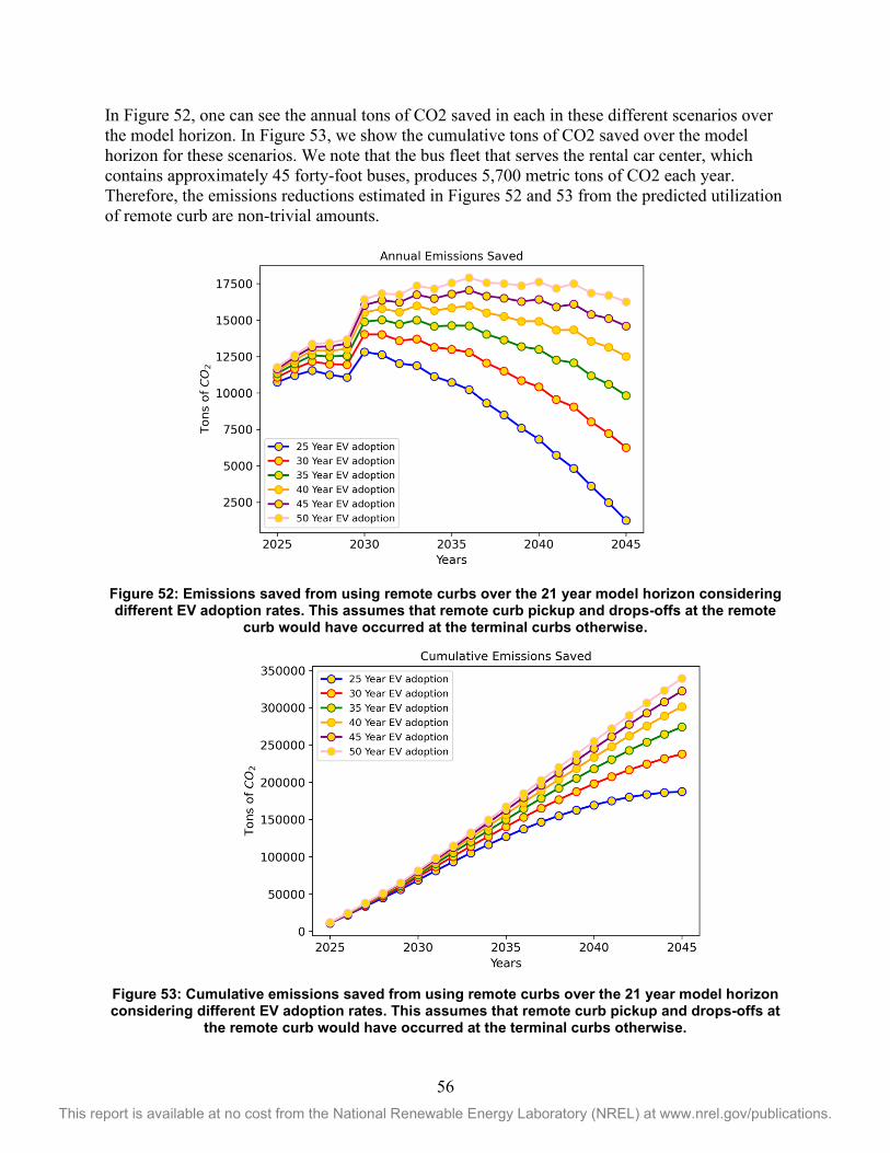
56 This report is available at no cost from the National Renewable Energy Laboratory (NREL) at www.nrel.gov/publications.
In Figure 52, one can see the annual tons of CO2 saved in each in these different scenarios over the model horizon. In Figure 53, we show the cumulative tons of CO2 saved over the model horizon for these scenarios. We note that the bus fleet that serves the rental car center, which contains approximately 45 forty-foot buses, produces 5,700 metric tons of CO2 each year. Therefore, the emissions reductions estimated in Figures 52 and 53 from the predicted utilization of remote curb are non-trivial amounts.
Figure 52: Emissions saved from using remote curbs over the 21 year model horizon considering different EV adoption rates. This assumes that remote curb pickup and drops-offs at the remote
curb would have occurred at the terminal curbs otherwise.
Figure 53: Cumulative emissions saved from using remote curbs over the 21 year model horizon considering different EV adoption rates. This assumes that remote curb pickup and drops-offs at
the remote curb would have occurred at the terminal curbs otherwise.

57 This report is available at no cost from the National Renewable Energy Laboratory (NREL) at www.nrel.gov/publications.
6.8 AV Scenario Analysis One goal of this work was to determine if the adoption of AVs in future years would change the prescribed infrastructure decisions from the model. In searching the literature for information and forecasts that would inform the construction of likely future AV scenarios, not much was found. Due to the lack of available information and forecasts, we decided to examine a few select cases that we thought would at least capture the range of possible effects from AVs on infrastructure needs. Towards this aim, we considered several AV scenarios as an extension of the baseline scenarios described above. In defining these AV scenarios, we made the following assumptions:
1. We assumed that AVs will be first adopted by TNCs at substantial levels, and thus, all AVs in our model are TNCs.
2. Significant adoption of AVs by TNCs does not occur before 2030. 3. The percentage of TNCs that are AVs increases linearly once adoption begins.
To capture AV effects in our model, we define a concept called AV vehicle equivalent (AVVE). We define AVVE as the number of non-autonomous vehicles an AV represents from a congestion perspective. For example, if AVVE = 0.8, then 100 AVs would be treated as 80 for the purpose computing congestion via the congestion functions derived from SUMO simulations: congestion = f(0.8*100).
We consider the scenarios described in Table 9, where each scenario is defines as a tuple (AVVE, Year AV adoption starts, annual percentage increase of AVs used by TNCs). We note that the use of 0.5 and 1.5 AVVE is extreme. This was deliberately done to have a very complete understanding of the range of effects TNC AVs could have on infrastructure needs.
Table 9: AV Adoption Scenarios
Optimistic AVVE Pessimistic AVVE
Fast adoption rate (0.5,2030,20% of TNCs) (1.5,2030,20% of TNCs)
Medium adoption rate (0.5,2035,10% of TNCs) (1.5,2035,10% of TNCs)
Slow adoption rate (0.5,2040,5% of TNCs) (1.5,2040,5% of TNCs)
We found that the six scenarios have similar build results for remote parking but quite different build results for remote curb. Figure 54 shows the remote curb build results for the six different AV scenarios. With slow AV adoption rate, both the optimistic AVVE and the pessimistic AVVE scenarios have identical remote curb build results as the basic scenario that does not consider AVs. This suggests that if AVs are adopted slowly regardless of their AVVE, the infrastructure build decisions will not be changed. For the scenario with optimistic AVVE and fast adoption and the scenario with optimistic AVVE and medium adoption, the remote curb build results are identical. Compared to the basic scenario, without considering AVs, these two scenarios have the same build decisions in construction years 2025, 2030, and 2035, but do not build remote curb spots in construction year 2040. For the scenario with pessimistic AVVE and fast adoption and the scenario with pessimistic AVVE and medium adoption, the south remote curb build results are identical to the basic scenario without AVs. For the north remote curb, the
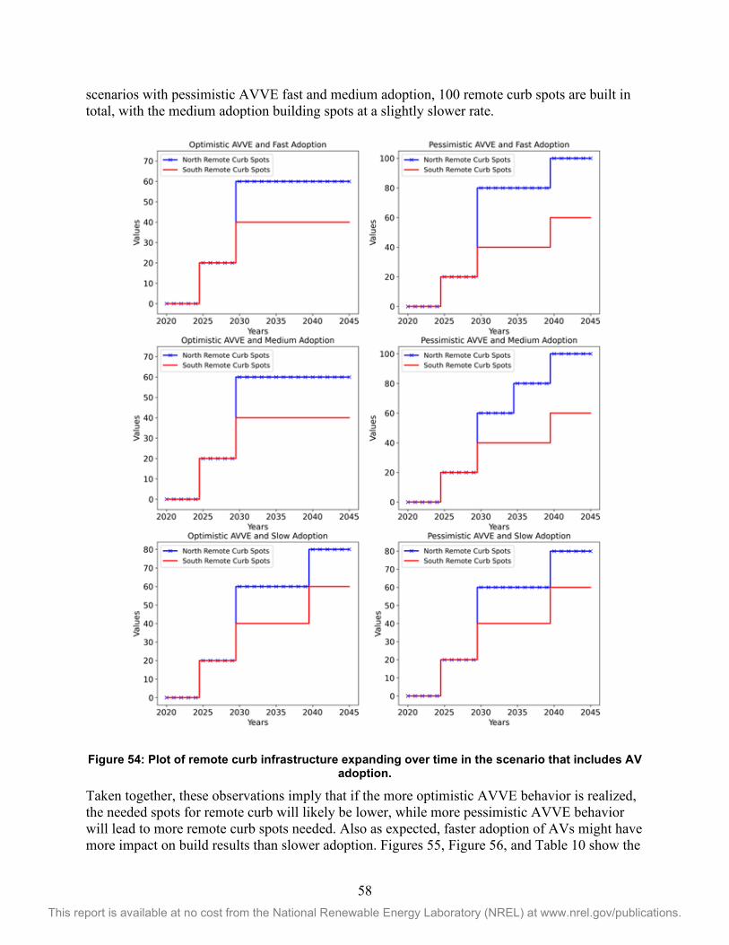
58 This report is available at no cost from the National Renewable Energy Laboratory (NREL) at www.nrel.gov/publications.
scenarios with pessimistic AVVE fast and medium adoption, 100 remote curb spots are built in total, with the medium adoption building spots at a slightly slower rate.
Figure 54: Plot of remote curb infrastructure expanding over time in the scenario that includes AV adoption.
Taken together, these observations imply that if the more optimistic AVVE behavior is realized, the needed spots for remote curb will likely be lower, while more pessimistic AVVE behavior will lead to more remote curb spots needed. Also as expected, faster adoption of AVs might have more impact on build results than slower adoption. Figures 55, Figure 56, and Table 10 show the

59 This report is available at no cost from the National Renewable Energy Laboratory (NREL) at www.nrel.gov/publications.
costs and revenue for different AV scenarios. One can see that although different AV scenarios have different costs and revenues, the differences are marginal. One potential reason for this is that we assume AVs are only adopted by TNCs and TNCs only account for a small portion of the total traffic volume. If personal AVs become widely adopted in the time frame considered the impact of AVs on infrastructure needs could be more significant.
Figure 55: Comparison of lifecycle costs for different AV scenarios.
Figure 56: Comparison of lifecycle revenue for different AV scenarios.
We note that these scenarios do not consider certain effects that AVs might have on mode choice. For example, AVs might lower the cost of TNCs, making it a more appealing mode choice. AVs might also change peoples’ perceived value of time, if AVs allow for people to be more productive on car rides, influencing future mode choice distributions. Additionally, we were not able to construct a special vehicle class in SUMO that could simulate the effects of AVs. This could potentially offer a better estimate of the true AVVE factor. Generally, this work has highlighted a need for work on forecasting AV adoption, simulating AV behavior at curb and broader road networks, as well as modeling how mode choice behavior might be influenced by having AV transportation options. Such research efforts could improve our ability to estimate the needed future infrastructure at DFW and other airports.

60 This report is available at no cost from the National Renewable Energy Laboratory (NREL) at www.nrel.gov/publications.
Table 10: Comparison of lifecycle costs and revenues for different AV scenarios
Scenarios Construction Cost ($106)
Operating Cost ($106)
Revenue ($106)
No AV Impact 303 1452 12458
Pessimistic AVVE and Slow Adoption 316 1440 12456
Pessimistic AVVE and Medium Adoption 322 1453 12465
Pessimistic AVVE and Fast Adoption 322 1456 12428
Optimistic AVVE and Slow Adoption 319 1439 12464
Optimistic AVVE and Medium Adoption 316 1425 12459
Optimistic AVVE and Fast Adoption 303 1436 12472
6.9 Terminal Capacity Sensitivity Analysis Our simulations show that the terminal area of DFW can handle approximately 6,000 vehicles entering it per hour before major congestion starts to occur. In Figure 57, the number of cars going into the DFW terminal area per hour is plotted against the average travel time it takes a car to visit a terminal curb and leave the airport. One can see that several outliers start to emerge between 5,000 and 6,000 vehicles per hour. This indicates that the SUMO simulation network is at capacity. However, several sources of uncertainty in this estimate must be addressed. First, from the data above, it could also be inferred that the terminal capacity is 5,500 vehicles per hour, and it is not completely clear from the simulation when severe congestion would begin. Another issue is that DFW currently has pass through traffic volume along International Parkway, which runs through the terminal area. It is unclear how this traffic volume will evolve in the future and how it will be affected by terminal congestion pricing. This traffic volume can be viewed as a reduction in the terminal capacity and provides uncertainty regarding what the true terminal capacity is. Additionally, DFW is planning substantial road network modifications to the terminal area ramps and bridges. At present all terminal off ramps from International Parkway to the terminals are on the left-hand side of International Parkway, and they are going to be moved to the right-hand side. It is not clear what effect this will have on the network capacity. We are also not considering the 6th terminal that DFW is planning to build at some point in the future, which could change the terminal network capacity as well as the needed capacity. Finally, our estimate of the terminal capacity does not consider weather events, traffic disruptions, or lane closures due to construction. These types of events can lower the network capacity temporally but might occur frequently enough to warrant consideration in the infrastructure planning process.

61 This report is available at no cost from the National Renewable Energy Laboratory (NREL) at www.nrel.gov/publications.
Figure 57: CTA flow capacity at DFW Airport derived from simulation.
To better understand how different capacity values for the DFW terminal area might influence the infrastructure recommendations from our model, we have done a sensitivity analysis of the infrastructure decisions. We consider another three cases with the terminal capacity being 4,000, 5,000, and 7,000 vehicles/hour, respectively. We found that, compared to the basic case (with terminal capacity being 6,000 vehicles/hour), the above three cases have identical solutions for the remote curb construction decisions, while they have slightly different solutions for the remote parking construction and shuttle purchase decisions. Figures 58, Figure 59, and Table 11 show the costs and revenue for different terminal capacity scenarios.
Figure 58: Comparison of lifecycle costs for different terminal capacity scenarios.
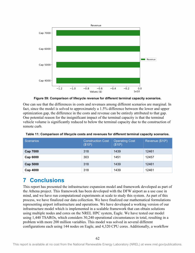
62 This report is available at no cost from the National Renewable Energy Laboratory (NREL) at www.nrel.gov/publications.
Figure 59: Comparison of lifecycle revenue for different terminal capacity scenarios.
One can see that the differences in costs and revenues among different scenarios are marginal. In fact, since the model is solved to approximately a 1.5% difference between the lower and upper optimization gap, the difference in the costs and revenue can be entirely attributed to that gap. One potential reason for the insignificant impact of the terminal capacity is that the terminal vehicle volume is significantly reduced to below the terminal capacity due to the construction of remote curb.
Table 11: Comparison of lifecycle costs and revenues for different terminal capacity scenarios.
Scenarios Construction Cost ($106)
Operating Cost ($106)
Revenue ($106)
Cap 7000 318 1439 12461
Cap 6000 303 1451 12457
Cap 5000 318 1439 12461
Cap 4000 318 1439 12461
7 Conclusions This report has presented the infrastructure expansion model and framework developed as part of the Athena project. This framework has been developed with the DFW airport as a use case in mind, and we have run computational experiments at scale to study this system. As part of this process, we have finalized our data collection. We have finalized our mathematical formulations representing airport infrastructure and operations. We have developed a working version of our infrastructure model which is implemented in a scalable framework that can obtain solutions using multiple nodes and cores on the NREL HPC system, Eagle. We have tested our model using 1,440 TSAROs, which considers 30,240 operational circumstances in total, resulting in a problem with more 200 million variables. This model was solved in several different configurations each using 144 nodes on Eagle, and 4,320 CPU cores. Additionally, a workflow

63 This report is available at no cost from the National Renewable Energy Laboratory (NREL) at www.nrel.gov/publications.
that enables us to simulate the performance of the infrastructure model results was developed and deployed on Eagle across multiple nodes.
We have run the standard version of our model to estimate the needed infrastructure at DFW from 2025 to 2045. We have also examined a select set of AV scenarios in order to estimate the effects on needed infrastructure from AVs. Additionally, we conducted a sensitivity analysis regarding the terminal area capacity at DFW to understand how uncertainties in that estimate might influence infrastructure needs. In general, our results indicate that a combination of remote parking, remote curb infrastructure, and dynamic pricing can generate revenue, reduce emissions, and manage airport passenger growth over time. We note the success of the proposed strategy depends on the data collection and forecasting abilities of DFW as was shown in Section 6.5.2. We have also seen that the AV adoption by TNCs might necessitate larger amounts of remote curb.
This work has left many avenues for further research. The results from section 6.6.2 indicate that the model likely underestimates the needed remote curb. This, we believe, is due to the two-stage nature of our model. Based on our work, we believe a three-stage model would yield better estimations of the needed remote curb infrastructure. However, our efforts to solve the three-stage version of our model were unsuccessful. Thus, new mathematical representations and algorithms are needed so solve three-stage versions of this model. This is one possible avenue for future research. Another difficulty that we faced was representing many airport subsystems within the same model and capturing those systems behavior and interactions within an algebraic modeling framework like Pyomo. One example of this challenge was building surrogate models to represent road network congestion using SUMO simulation data in such a way that the surrogate models could embedded into a Pyomo model using algebraic equations. Research into this question alone would be valuable. Another example along these lines is how to represent parking lot occupancy levels well enough, algebraically, to determine in which hours parking might overflow. Errors in these estimates can result in errors in the prescribed expansion of parking. Thus, a possible area of future research is determining different ways that algebraic constraints can be used to better estimate the dynamics and state behavior in parking lots. A third example is how pricing influences on mode choice behavior can be captured in detail within an algebraic model. These challenges regarding embedding subsystem representations into an algebraic modeling framework so that power commercial branch and bound algorithms can be leveraged begs the question, “Is an algebraic modeling framework the correct framework to be investigating these airport infrastructure expansion questions?” It is likely that direct simulation or more advanced machine learning based surrogate models could better capture mode choice, parking, and traffic network behavior. This would come at the cost of having a less sophisticated optimization framework to leverage these simulations or advanced surrogate models, and the optimization framework used would likely lack optimality guarantees. Still research that explores the trade-off between the quality of the optimization framework and the quality of the surrogate model representation of sub-system behavior would be of value.

64 This report is available at no cost from the National Renewable Energy Laboratory (NREL) at www.nrel.gov/publications.
References Ashford, Norman J., Saleh Mumayiz, and Paul H. Wright. Airport engineering: planning, design, and development of 21st century airports. John Wiley & Sons, 2011.
Asian Development Bank . Sustainable Transport Solutions: Low-Carbon Buses in the People’s
Republic of China. Asian Development Bank (2018). http://dx.doi.org/10.22617/TCS189646-2.
H M Abdul Aziz, Xiaodan Xu, Yanbo Ge, Michael Hillard, Caleb Phillips. :Modeling Travel Mode Choices Near Transportation Hubs: The Case of Dallas-Fort Worth Airport using Revealed Survey Data.” Presented at 99th TRB Annual Meeting. January 12-16, 2020.
Birge, John R., and Francois Louveaux. Introduction to stochastic programming. Springer Science & Business Media, 2011.
Broin, Eoin Ó., and Céline Guivarch. "Transport infrastructure costs in low-carbon pathways." Transportation Research Part D: Transport and Environment 55 (2017): 389-403.
Bushell, Max A., Bryan W. Poole, Charles V. Zegeer, and Daniel A. Rodriguez. "Costs for pedestrian and bicyclist infrastructure improvements." University of North Carolina Highway Safety Research Center, University of North Carolina, Chapel Hill 45 (2013).
Dunning, Iain, Joey Huchette, and Miles Lubin. "JuMP: A modeling language for mathematical optimization." SIAM Review 59, no. 2 (2017): 295-320.
FAA Aerospace Forecast Report for 2019-2039 https://www.faa.gov/data_research/aviation/aerospace_forecasts/media/FAA_Aerospace_Forecasts_FY_2019-2039.pdf
Ge, Yanbo, Alec Biehl, Srinath Ravulaparthy, Venu Garikapati, Monte Lunacek, and Caleb Phillips. “Joint Modeling of Access Mode and Parking Choice of Air Travelers Using Revealed Preference Data.” Transportation Research Record, (July 2021). https://doi.org/10.1177/03611981211019037.
Hart, William E., Carl D. Laird, Jean-Paul Watson, David L. Woodruff, Gabriel A. Hackebeil, Bethany L. Nicholson, and John D. Siirola. Pyomo-optimization modeling in python. Vol. 67. Berlin: Springer, 2017.
Hart, William E., Jean-Paul Watson, and David L. Woodruff. "Pyomo: modeling and solving mathematical programs in Python." Mathematical Programming Computation 3, no. 3 (2011): 219.
Henao, A., Sperling, J., Garikapati, V., Hou, Y., Young, S.. Airport Analyses Informing New Mobility Shifts: Opportunities to Adapt Energy-Efficient Mobility Services and Infrastructure. Intelligent Transportation Society of America. 2018 Annual Meeting. Detroit, Michigan. June 4-7, 2018. https://www.nrel.gov/docs/fy18osti/71036.pdf

65 This report is available at no cost from the National Renewable Energy Laboratory (NREL) at www.nrel.gov/publications.
Helber, Stefan, Justine Broihan, Young Jae Jang, Peter Hecker, and Thomas Feuerle. "Location planning for dynamic wireless charging systems for electric airport passenger buses." Energies 11, no. 2 (2018): 258.
Huchette, Joey, Miles Lubin, and Cosmin Petra. "Parallel algebraic modeling for stochastic optimization." In Proceedings of the 1st First Workshop for High Performance Technical Computing in Dynamic Languages, pp. 29-35. IEEE Press, 2014.
Johnson, Caley, Erin Nobler, Leslie Eudy, and Matthew Jeffers. Financial Analysis of Battery Electric Transit Buses. No. NREL/TP-5400-74832. 2020.
Kotz A, Ficenec K, Kelly K, Berger S. Electrification of Airport Shuttle Operations. InProceedings of the 33rd Electric Vehicle Symposium 2020 Sep 13.
Lawrence, Brianna. (2020). Electric Shuttles are Taking Off at Airports. https://www.act-news.com/news/electric-shuttles-are-taking-off-at-airports/ (Accessed July 2020)
Lopez, Pablo Alvarez, Michael Behrisch, Laura Bieker-Walz, Jakob Erdmann, Yun-Pang Flötteröd, Robert Hilbrich, Leonhard Lücken, Johannes Rummel, Peter Wagner, and Evamarie WieBner. "Microscopic traffic simulation using sumo." In 2018 21st International Conference on Intelligent Transportation Systems (ITSC), pp. 2575-2582. IEEE, 2018.
Matloff, Norm. "Introduction to discrete-event simulation and the simpy language." Davis, CA. Dept of Computer Science. University of California at Davis. Retrieved on August 2, no. 2009 (2008): 1-33.
Munoz, Francisco D., and Jean-Paul Watson. "A scalable solution framework for stochastic transmission and generation planning problems." Computational Management Science 12, no. 4 (2015): 491-518.
Nelson, Barry. Foundations and methods of stochastic simulation: a first course. Springer Science & Business Media, 2013.
Quarles, Neil, Kara M. Kockelman, and Moataz Mohamed. "Costs and Benefits of Electrifying and Automating Bus Transit Fleets." Sustainability 12, no. 10 (2020): 3977.
R. T. Rockafellar. Optimization under uncertainty,” lecture notes, 2001.
Rockafellar, R. Tyrrell, and Roger J-B. Wets. "Scenarios and policy aggregation in optimization under uncertainty." Mathematics of operations research 16, no. 1 (1991): 119-147.
Safta, Cosmin, Richard L-Y. Chen, Habib N. Najm, Ali Pinar, and Jean-Paul Watson. "Toward using surrogates to accelerate solution of stochastic electricity grid operations problems." In 2014 North American Power Symposium (NAPS), pp. 1-6. IEEE, 2014.
Sigler, Devon., Andrew Kotz, Qichao Wang, Zhaocai Liu, Kenneth Kelly, Monte Lunacek, and Caleb Phillips. 6.3.2.1 – ATHENA – Milestone 1.2: M6 - Results from bus electrification and route optimization. NREL. 2020.

66 This report is available at no cost from the National Renewable Energy Laboratory (NREL) at www.nrel.gov/publications.
Sigler, Devon, Qichao Wang, Zhaocai Liu, Venu Garikapati, Andrew Kotz, Kenneth J. Kelly, Monte Lunacek, Caleb Phillips, Route optimization for energy efficient airport shuttle operations – A case study from Dallas Fort worth International Airport. Journal of Air Transport Management. Volume 94. 2021.
Sun, Yanshuo, and Paul Schonfeld. "Stochastic capacity expansion models for airport facilities." Transportation Research Part B: Methodological 80 (2015): 1-18.
Wächter, Andreas, and Lorenz T. Biegler. "On the implementation of an interior-point filter line-search algorithm for large-scale nonlinear programming." Mathematical programming 106, no. 1 (2006): 25-57.
Watson, Jean-Paul, David L. Woodruff, and William E. Hart. "PySP: modeling and solving stochastic programs in Python." Mathematical Programming Computation 4, no. 2 (2012): 109-149

67 This report is available at no cost from the National Renewable Energy Laboratory (NREL) at www.nrel.gov/publications.
Appendix A. Two Stage Stochastic Model In this section, we present the mathematical model we have developed for carrying out the modeling approach described in this report. It is a scenario-based two stage model. We first present the sets, parameters, variables, and functions used in the model. We then break the variables up according to the stages they belong to. Finally, we present the objective function and the constraints according to the stages they belong to.
Table A1: Sets, Parameters, and Variables
Sets Description
𝑌𝑌 Set of years within the planning horizon
𝑌𝑌𝐶𝐶𝐶𝐶𝐶𝐶 Set of years construction can occur
𝑇𝑇 Set of trajectories for future passenger growth as well as EV (or emissions reductions) and AV technology adoption
𝐻𝐻 Set of hours used to represent airport conditions throughout the year
𝐿𝐿𝐷𝐷𝐷𝐷𝐷𝐷𝐷𝐷𝐷𝐷 Set of site areas where delay or congestion is measured
𝐿𝐿𝑅𝑅𝑅𝑅 Set of remote parking sites
𝐿𝐿𝑋𝑋𝑅𝑅 Set of express parking sites
𝐿𝐿𝑇𝑇𝑅𝑅 Set of terminal area parking sites
𝐿𝐿𝑅𝑅 𝐿𝐿𝑅𝑅𝑅𝑅 ∪ 𝐿𝐿𝑋𝑋𝑅𝑅 ∪ 𝐿𝐿𝑇𝑇𝑅𝑅
𝐿𝐿𝑆𝑆 Set of sites that shuttle passengers to the terminals, (e.g., remote curbs, remote parking, express parking)
𝐿𝐿𝑆𝑆𝑆𝑆𝐷𝐷𝑆𝑆 ⊆ 𝐿𝐿𝑆𝑆 Set of currently nonexistent sites that shuttle passengers to the terminals
𝑁𝑁𝐷𝐷𝑆𝑆 Set of shuttle routes for shuttle service site 𝑙𝑙 ∈ 𝐿𝐿𝑆𝑆, (we assume that the sets 𝑁𝑁𝐷𝐷𝑆𝑆 form a partition of the routes used at the airport, hence no route serves two sites in 𝐿𝐿𝑆𝑆)
𝐿𝐿𝐶𝐶𝐶𝐶𝐶𝐶𝑅𝑅 ⊆ 𝐿𝐿𝑅𝑅 Set of potential parking construction sites
𝐿𝐿𝐶𝐶𝐶𝐶𝐶𝐶𝑅𝑅𝑆𝑆𝐷𝐷𝑆𝑆 ⊆ 𝐿𝐿𝐶𝐶𝐶𝐶𝐶𝐶𝑅𝑅 Set of potential parking construction sites that are currently nonexistent.
𝐿𝐿𝐶𝐶𝐶𝐶𝐶𝐶𝑅𝑅𝐶𝐶 Set of potential remote curb construction sites
𝐿𝐿𝐶𝐶𝐶𝐶 ⊆ 𝐿𝐿𝑅𝑅 Set of potential construction sites for converting parking to curb
𝛱𝛱
Set of potential final construction combinations specifying which currently-nonexistent construction sites are built and the year those sites are initially constructed, e.g., a new parking site 𝑙𝑙∗ ∈ 𝐿𝐿𝐶𝐶𝐶𝐶𝐶𝐶𝑅𝑅 is constructed at the first construction year and no new remote curb sites are constructed throughout the planning horizon.
𝛱𝛱𝐷𝐷,𝐷𝐷𝑆𝑆 Set of potential final construction combinations where shuttle site 𝑙𝑙 ∈ 𝐿𝐿𝑆𝑆 exists by year 𝑦𝑦 ∈ 𝑌𝑌
𝑀𝑀 Set of mode choices for passengers to get to and from the airport, for modeling simplicity we make these mode choices location specific
𝐴𝐴 Set of sets 𝐴𝐴(𝐶𝐶, ℎ)
𝐴𝐴(𝐶𝐶, ℎ) Set of stochastic scenarios which describe different congestion price responses, and the resulting mode choice volumes and associated revenue. There exists one

68 This report is available at no cost from the National Renewable Energy Laboratory (NREL) at www.nrel.gov/publications.
of these scenario sets for each trajectory 𝐶𝐶 ∈ 𝑇𝑇, and hour ℎ ∈ 𝐻𝐻. Thus, it is a finite scenario based representation of a conditional distribution, which is conditioned on the respective hour, and trajectory
𝑄𝑄𝑅𝑅𝑅𝑅 Set indexing the remote parking pricing options
𝑄𝑄𝑇𝑇𝑅𝑅 Set indexing the terminal area parking pricing options
𝑄𝑄𝐶𝐶𝐶𝐶𝐶𝐶𝐶𝐶 Set indexing the congestion pricing options
Scalar Parameters Description
𝜃𝜃 Discount rate (year-based) for life cycle cost evaluation
𝑝𝑝𝑇𝑇𝑅𝑅𝑇𝑇𝑇𝑇 Penalty for total parking overflow across all parking sites
𝜔𝜔 Weight of each hour scenario. Should always be 8760
𝑟𝑟𝑆𝑆𝐶𝐶𝑆𝑆 The number of remote curb spots that require a new car lane for in and out flowing traffic
𝑟𝑟𝑆𝑆𝑆𝑆𝑆𝑆 The number of remote curb spots that require a new bus lane for shuttle service
𝑟𝑟𝑆𝑆𝐶𝐶𝑅𝑅𝑅𝑅 The number of remote curb spots that require one cell phone parking spot
𝜁𝜁𝑅𝑅𝐶𝐶 Increment in which remote curb must be built in a construction year
𝜁𝜁𝑅𝑅 Increment in which parking must be built in a construction year
𝜁𝜁𝐶𝐶𝑅𝑅𝑅𝑅 Increment in which cell phone parking must be built in a construction year
𝜁𝜁𝐶𝐶𝐶𝐶 Increment in which parking spots must be converted to curb in a construction year
𝜁𝜁𝐶𝐶𝑆𝑆 Increment in which car lanes must be built in a construction year
𝜁𝜁𝑆𝑆𝑆𝑆 Increment in which bus lanes must be built in a construction year
𝜁𝜁𝐶𝐶𝐶𝐶𝐶𝐶 Increment in which electric bus chargers must be installed in a construction year
𝜁𝜁𝑆𝑆 Increment in which electric buses must be purchased in a construction year
𝑟𝑟𝑆𝑆𝐶𝐶𝐶𝐶𝐶𝐶 Ratio determining the number of chargers needed to serve a certain number of electric buses
𝑟𝑟𝑆𝑆𝑇𝑇 Ratio of total bus fleet with active fleet needed to ensure the active fleet is possible given charging constraints
𝑟𝑟𝐶𝐶𝐶𝐶 The number of parking spots needed to create a new converted pickup/drop-off spot
Set Dependent Parameters Description
𝑝𝑝𝐷𝐷𝑅𝑅𝑇𝑇𝑇𝑇 Penalty for parking overflow at parking site 𝑙𝑙 ∈ 𝐿𝐿𝑅𝑅
𝑝𝑝𝐶𝐶𝑆𝑆𝑇𝑇𝑇𝑇−𝐼𝐼𝑆𝑆 Penalty for leaving people behind waiting for a shuttle going to a terminal for shuttle route 𝑛𝑛 ∈ 𝑁𝑁𝐷𝐷𝑆𝑆, where 𝑙𝑙 ∈ 𝐿𝐿𝑆𝑆
𝑝𝑝𝐶𝐶𝑆𝑆𝑇𝑇𝑇𝑇−𝑇𝑇𝑂𝑂𝑇𝑇 Penalty for leaving people behind waiting for a shuttle to leave a terminal for shuttle route 𝑛𝑛 ∈ 𝑁𝑁𝐷𝐷𝑆𝑆, where 𝑙𝑙 ∈ 𝐿𝐿𝑆𝑆
𝑧𝑧𝐷𝐷𝐶𝐶𝐶𝐶𝐶𝐶𝐷𝐷𝐶𝐶 Max number of spots allowed to be converted from parking to pickup/drop-off spots at site 𝑙𝑙 ∈ 𝐿𝐿𝐶𝐶𝐶𝐶
𝑐𝑐𝐷𝐷,𝐷𝐷𝑅𝑅 Construction cost per parking spot at 𝑙𝑙 ∈ 𝐿𝐿𝐶𝐶𝐶𝐶𝐶𝐶𝑅𝑅 and 𝑦𝑦 ∈ 𝑌𝑌𝐶𝐶𝐶𝐶𝐶𝐶

69 This report is available at no cost from the National Renewable Energy Laboratory (NREL) at www.nrel.gov/publications.
𝑐𝑐𝐷𝐷,𝐷𝐷𝑅𝑅𝐶𝐶 Construction cost per remote curb spot at 𝑙𝑙 ∈ 𝐿𝐿𝐶𝐶𝐶𝐶𝐶𝐶𝑅𝑅𝐶𝐶 and 𝑦𝑦 ∈ 𝑌𝑌𝐶𝐶𝐶𝐶𝐶𝐶
𝑐𝑐𝐷𝐷,𝐷𝐷𝐶𝐶𝐶𝐶 Construction cost to convert parking to pickup/drop-off area at 𝑙𝑙 ∈ 𝐿𝐿𝐶𝐶𝐶𝐶 and 𝑦𝑦 ∈𝑌𝑌𝐶𝐶𝐶𝐶𝐶𝐶
𝑐𝑐𝐷𝐷,𝐷𝐷𝑆𝑆 Construction cost per lane of connecting road at remote curb site 𝑙𝑙 ∈ 𝐿𝐿𝐶𝐶𝐶𝐶𝐶𝐶𝑅𝑅𝐶𝐶 and 𝑦𝑦 ∈ 𝑌𝑌𝐶𝐶𝐶𝐶𝐶𝐶
𝑐𝑐𝐷𝐷,𝐷𝐷𝑆𝑆 Purchase cost of an electric bus for 𝑙𝑙 ∈ 𝐿𝐿𝐶𝐶𝐶𝐶𝐶𝐶𝑅𝑅𝐶𝐶 ∪ 𝐿𝐿𝐶𝐶𝐶𝐶𝐶𝐶𝑅𝑅 and 𝑦𝑦 ∈ 𝑌𝑌𝐶𝐶𝐶𝐶𝐶𝐶
𝑐𝑐𝐷𝐷,𝐷𝐷𝐶𝐶𝐶𝐶𝐶𝐶 Cost of an electric bus charger for 𝑙𝑙 ∈ 𝐿𝐿𝐶𝐶𝐶𝐶𝐶𝐶𝑅𝑅𝐶𝐶 ∪ 𝐿𝐿𝐶𝐶𝐶𝐶𝐶𝐶𝑅𝑅 and 𝑦𝑦 ∈ 𝑌𝑌𝐶𝐶𝐶𝐶𝐶𝐶
𝑐𝑐𝐷𝐷𝑅𝑅𝐷𝐷𝑡𝑡𝑖𝑖𝐶𝐶 Cost reduction ratio to scale the cost based on the limited modeled benefit captured in the optimization horizon 𝑦𝑦 ∈ 𝑌𝑌𝐶𝐶𝐶𝐶𝐶𝐶
𝑧𝑧𝜋𝜋,𝐷𝐷,𝐷𝐷𝑅𝑅𝑃𝑃𝑖𝑖𝐶𝐶
The minimum number of parking spots required at site 𝑙𝑙 ∈ 𝐿𝐿𝑅𝑅 in year 𝑦𝑦 ∈ 𝑌𝑌 considering the final construction combination of currently nonexistent construction sites is 𝜋𝜋 ∈ 𝛱𝛱
𝑧𝑧𝜋𝜋,𝐷𝐷,𝐷𝐷𝑅𝑅𝐶𝐶𝑃𝑃𝑖𝑖𝐶𝐶
The minimum number of remote curb spots required at site 𝑙𝑙 ∈ 𝐿𝐿𝑅𝑅 in year 𝑦𝑦 ∈ 𝑌𝑌 considering the final construction combination of currently nonexistent construction sites is 𝜋𝜋 ∈ 𝛱𝛱
𝑧𝑧𝐷𝐷𝑅𝑅0 Number of parking spots available initially at site 𝑙𝑙 ∈ 𝐿𝐿𝑅𝑅
𝑧𝑧𝐷𝐷𝑅𝑅𝐶𝐶0 Number of remote curb spots available initially at site 𝑙𝑙 ∈ 𝐿𝐿𝐶𝐶𝐶𝐶𝐶𝐶𝑅𝑅𝐶𝐶
𝑧𝑧𝐷𝐷𝐶𝐶𝐶𝐶0 Number of pickup and drop-off spots available initially at parking to curb conversion site 𝑙𝑙 ∈ 𝐿𝐿𝐶𝐶𝐶𝐶
𝑧𝑧𝐶𝐶,𝐷𝐷𝑆𝑆0 Number of shuttle buses available for shuttling passengers for shuttle route
𝑛𝑛 ∈ 𝑁𝑁𝐷𝐷𝑆𝑆, where 𝑙𝑙 ∈ 𝐿𝐿𝑆𝑆
𝐶𝐶𝐶𝐶,𝐷𝐷,𝐷𝐷,ℎ𝑃𝑃𝑖𝑖𝐶𝐶 Lower bound on number of shuttle buses in service in year 𝑦𝑦 ∈ 𝑌𝑌, hour ℎ ∈ 𝐻𝐻 for
shuttle route 𝑛𝑛 ∈ 𝑁𝑁𝐷𝐷𝑆𝑆, where 𝑙𝑙 ∈ 𝐿𝐿𝑆𝑆
𝐶𝐶𝐶𝐶,𝐷𝐷𝐶𝐶𝐷𝐷𝐶𝐶 Capacity for shuttle bus serving route 𝑛𝑛 ∈ 𝑁𝑁𝐷𝐷𝑆𝑆, where 𝑙𝑙 ∈ 𝐿𝐿𝑆𝑆
𝑐𝑐𝐷𝐷,𝐷𝐷𝑇𝑇𝑅𝑅𝐶𝐶 Hourly remote curb operation cost per remote curb spots in year 𝑦𝑦 ∈ 𝑌𝑌 for site 𝑙𝑙 ∈𝐿𝐿𝐶𝐶𝐶𝐶𝐶𝐶𝑅𝑅𝐶𝐶
𝑐𝑐𝐶𝐶,𝐷𝐷,𝐷𝐷𝑇𝑇𝑆𝑆 Hourly shuttle bus operation cost per bus in year 𝑦𝑦 ∈ 𝑌𝑌 for shuttle route 𝑛𝑛 ∈ 𝑁𝑁𝐷𝐷𝑆𝑆,
where 𝑙𝑙 ∈ 𝐿𝐿𝑆𝑆
𝑓𝑓𝐶𝐶,𝐷𝐷,𝐷𝐷,𝑡𝑡,ℎ,𝑠𝑠𝑆𝑆 The number of loops per hour a bus makes servicing shuttle route 𝑛𝑛 ∈ 𝑁𝑁𝐷𝐷𝑆𝑆, where
𝑙𝑙 ∈ 𝐿𝐿𝑆𝑆, year 𝑦𝑦 ∈ 𝑌𝑌, trajectory 𝐶𝐶 ∈ 𝑇𝑇, hour ℎ ∈ 𝐻𝐻, and scenario 𝐶𝐶 ∈ 𝐴𝐴(𝐶𝐶, ℎ)
𝑣𝑣𝜋𝜋,𝐶𝐶,𝐷𝐷,𝑡𝑡,ℎ,𝑠𝑠,𝑖𝑖,𝑖𝑖,𝑘𝑘𝑅𝑅𝐷𝐷𝑃𝑃
Volume parameter for mode 𝑇𝑇 ∈ 𝑀𝑀, year 𝑦𝑦 ∈ 𝑌𝑌, trajectory 𝐶𝐶 ∈ 𝑇𝑇, hour ℎ ∈ 𝐻𝐻, and scenario 𝐶𝐶 ∈ 𝐴𝐴(𝐶𝐶, ℎ) given remote parking, terminal parking, and congestion pricing options 𝑇𝑇, 𝑗𝑗, 𝑘𝑘 respectively, and considering the final construction combination of currently nonexistent construction sites to be 𝜋𝜋 ∈ 𝛱𝛱
𝑣𝑣𝐷𝐷,𝑡𝑡,ℎ,𝑠𝑠𝑇𝑇𝐶𝐶𝑡𝑡𝑅𝑅𝐷𝐷𝑃𝑃 Total volume parameter for year 𝑦𝑦 ∈ 𝑌𝑌, trajectory 𝐶𝐶 ∈ 𝑇𝑇, hour ℎ ∈ 𝐻𝐻, and scenario
𝐶𝐶 ∈ 𝐴𝐴(𝐶𝐶, ℎ)
𝑇𝑇𝜋𝜋,𝐷𝐷,𝑡𝑡,ℎ,𝑠𝑠,𝑖𝑖,𝑖𝑖,𝑘𝑘𝑅𝑅𝐷𝐷𝑃𝑃
Revenue for year 𝑦𝑦 ∈ 𝑌𝑌, trajectory 𝐶𝐶 ∈ 𝑇𝑇, hour ℎ ∈ 𝐻𝐻, and scenario 𝐶𝐶 ∈ 𝐴𝐴(𝐶𝐶, ℎ) given remote parking, terminal parking, and congestion pricing options 𝑇𝑇, 𝑗𝑗, 𝑘𝑘 respectively, and considering the final construction combination of currently nonexistent construction sites to be 𝜋𝜋 ∈ 𝛱𝛱
𝑐𝑐𝐷𝐷𝐶𝐶𝑇𝑇𝑇𝑇 Peoples’ value of time using the airport for year 𝑦𝑦 ∈ 𝑌𝑌

70 This report is available at no cost from the National Renewable Energy Laboratory (NREL) at www.nrel.gov/publications.
𝑎𝑎𝐷𝐷𝐷𝐷𝐷𝐷𝐷𝐷𝐷𝐷𝐷𝐷 Average delay allowed at congestion site 𝑙𝑙 ∈ 𝐿𝐿𝐷𝐷𝐷𝐷𝐷𝐷𝐷𝐷𝐷𝐷
𝑷𝑷𝑷𝑷𝑷𝑷𝑷𝑷𝒕𝒕,𝒉𝒉,𝒔𝒔 The probability of scenario 𝐶𝐶 ∈ 𝐴𝐴(𝐶𝐶, ℎ) for trajectory 𝐶𝐶 ∈ 𝑇𝑇 and hour ℎ ∈ 𝐻𝐻
𝝉𝝉𝒊𝒊𝑹𝑹𝑷𝑷𝑷𝑷𝑹𝑹𝑷𝑷 Remote parking price option 𝑇𝑇 for 𝑇𝑇 ∈ 𝑄𝑄𝑅𝑅𝑅𝑅
𝝉𝝉𝒋𝒋𝑻𝑻𝑷𝑷𝑷𝑷𝑹𝑹𝑷𝑷 Terminal area parking price option 𝑗𝑗 for 𝑗𝑗 ∈ 𝑄𝑄𝑇𝑇𝑅𝑅
𝝉𝝉𝒌𝒌𝑪𝑪𝑷𝑷𝑪𝑪𝑪𝑪𝑷𝑷𝑹𝑹𝑷𝑷 Congestion price option 𝑘𝑘 for 𝑘𝑘 ∈ 𝑄𝑄𝐶𝐶𝐶𝐶𝐶𝐶𝐶𝐶
First Stage Variables Description
𝜓𝜓𝜋𝜋 Binary variable representing whether 𝜋𝜋 ∈ 𝛱𝛱 is the final construction combination of currently nonexistent construction sites
𝝍𝝍 A vector of {⋯ ,𝜓𝜓𝜋𝜋 ,⋯ }
𝑥𝑥𝐷𝐷,𝐷𝐷𝑅𝑅 Integer variable representing the number of parking spot increments built at site 𝑙𝑙 ∈ 𝐿𝐿𝐶𝐶𝐶𝐶𝐶𝐶𝑅𝑅 in construction year 𝑦𝑦 ∈ 𝑌𝑌𝐶𝐶𝐶𝐶𝐶𝐶
𝑥𝑥𝐷𝐷,𝐷𝐷𝑅𝑅𝐶𝐶 Integer variable representing the number of remote curb spot increments built at site 𝑙𝑙 ∈ 𝐿𝐿𝐶𝐶𝐶𝐶𝐶𝐶𝑅𝑅𝐶𝐶 in construction year 𝑦𝑦 ∈ 𝑌𝑌𝐶𝐶𝐶𝐶𝐶𝐶
𝑥𝑥𝐷𝐷,𝐷𝐷𝐶𝐶𝐶𝐶 Integer variable representing the number of increments of pickup and drop-off parking conversions at site 𝑙𝑙 ∈ 𝐿𝐿𝐶𝐶𝐶𝐶𝐶𝐶𝑅𝑅𝐶𝐶 in construction year 𝑦𝑦 ∈ 𝑌𝑌𝐶𝐶𝐶𝐶𝐶𝐶
𝑥𝑥𝐷𝐷,𝐷𝐷𝐶𝐶𝑆𝑆 Integer variable representing the number of car lanes built at site 𝑙𝑙 ∈ 𝐿𝐿𝐶𝐶𝐶𝐶𝐶𝐶𝑅𝑅𝐶𝐶 in construction year 𝑦𝑦 ∈ 𝑌𝑌𝐶𝐶𝐶𝐶𝐶𝐶
𝑥𝑥𝐷𝐷,𝐷𝐷𝑆𝑆𝑆𝑆 Integer variable representing the number of bus lanes built at site 𝑙𝑙 ∈ 𝐿𝐿𝐶𝐶𝐶𝐶𝐶𝐶𝑅𝑅𝐶𝐶 in construction year 𝑦𝑦 ∈ 𝑌𝑌𝐶𝐶𝐶𝐶𝐶𝐶
𝑥𝑥𝐷𝐷,𝐷𝐷𝐶𝐶𝑅𝑅𝑅𝑅 Integer variable representing the number of cell phone parking spots built at site 𝑙𝑙 ∈ 𝐿𝐿𝐶𝐶𝐶𝐶𝐶𝐶𝑅𝑅𝐶𝐶 in construction year 𝑦𝑦 ∈ 𝑌𝑌𝐶𝐶𝐶𝐶𝐶𝐶
𝑥𝑥𝐶𝐶,𝐷𝐷,𝐷𝐷𝑆𝑆 Integer variable representing the number of electric buses purchased for
supporting shuttle route 𝑛𝑛 ∈ 𝑁𝑁𝐷𝐷𝑆𝑆, 𝑙𝑙 ∈ 𝐿𝐿𝐶𝐶𝐶𝐶𝐶𝐶𝑅𝑅𝐶𝐶 ∪ 𝐿𝐿𝐶𝐶𝐶𝐶𝐶𝐶𝑅𝑅 in construction year 𝑦𝑦 ∈ 𝑌𝑌𝐶𝐶𝐶𝐶𝐶𝐶
𝑥𝑥𝐷𝐷,𝐷𝐷𝐶𝐶𝐶𝐶𝐶𝐶 Integer variable representing the number of electric buses chargers installed for supporting shuttle at site 𝑙𝑙 ∈ 𝐿𝐿𝐶𝐶𝐶𝐶𝐶𝐶𝑅𝑅𝐶𝐶 ∪ 𝐿𝐿𝐶𝐶𝐶𝐶𝐶𝐶𝑅𝑅 in construction year 𝑦𝑦 ∈ 𝑌𝑌𝐶𝐶𝐶𝐶𝐶𝐶
𝑧𝑧𝐷𝐷,𝐷𝐷𝑅𝑅 Integer variable representing the cumulative number of parking spots added at site 𝑙𝑙 ∈ 𝐿𝐿𝐶𝐶𝐶𝐶𝐶𝐶𝑅𝑅 in year 𝑦𝑦 ∈ 𝑌𝑌
𝑧𝑧𝐷𝐷,𝐷𝐷𝑅𝑅𝐶𝐶 Integer variable representing the cumulative number of remote curb spots added at site 𝑙𝑙 ∈ 𝐿𝐿𝐶𝐶𝐶𝐶𝐶𝐶𝑅𝑅𝐶𝐶 in year 𝑦𝑦 ∈ 𝑌𝑌
𝑧𝑧𝐷𝐷,𝐷𝐷𝐶𝐶𝐶𝐶 Integer variable representing the cumulative number of pickup and drop-off parking converted spots added at site 𝑙𝑙 ∈ 𝐿𝐿𝐶𝐶𝐶𝐶 in year 𝑦𝑦 ∈ 𝑌𝑌
𝑧𝑧𝐷𝐷,𝐷𝐷𝐶𝐶𝑆𝑆 Integer variable representing the cumulative number of car lanes added at site 𝑙𝑙 ∈𝐿𝐿𝐶𝐶𝐶𝐶𝐶𝐶𝑅𝑅𝐶𝐶 in year 𝑦𝑦 ∈ 𝑌𝑌
𝑧𝑧𝐷𝐷,𝐷𝐷𝑆𝑆𝑆𝑆 Integer variable representing the cumulative number of bus lanes added at site 𝑙𝑙 ∈ 𝐿𝐿𝐶𝐶𝐶𝐶𝐶𝐶𝑅𝑅𝐶𝐶 in year 𝑦𝑦 ∈ 𝑌𝑌
𝑧𝑧𝐷𝐷,𝐷𝐷𝐶𝐶𝑅𝑅𝑅𝑅 Integer variable representing the cumulative number of cell phone parking spots added at site 𝑙𝑙 ∈ 𝐿𝐿𝐶𝐶𝐶𝐶𝐶𝐶𝑅𝑅𝐶𝐶 in year 𝑦𝑦 ∈ 𝑌𝑌
𝑧𝑧𝐶𝐶,𝐷𝐷,𝐷𝐷𝑆𝑆 Integer variable representing the cumulative number of buses added for
supporting shuttling for shuttle route 𝑛𝑛 ∈ 𝑁𝑁𝐷𝐷𝑆𝑆, where 𝑙𝑙 ∈ 𝐿𝐿𝑆𝑆 in year 𝑦𝑦 ∈ 𝑌𝑌

71 This report is available at no cost from the National Renewable Energy Laboratory (NREL) at www.nrel.gov/publications.
𝑧𝑧𝐷𝐷,𝐷𝐷𝐶𝐶𝐶𝐶𝐶𝐶 Integer variable representing the cumulative number of electric buses chargers added for supporting shuttling at site 𝑙𝑙 ∈ 𝐿𝐿𝑆𝑆 in year 𝑦𝑦 ∈ 𝑌𝑌
Second Stage Variables Description
𝜔𝜔𝜋𝜋,𝐷𝐷,𝑡𝑡,ℎ,𝑖𝑖,𝑖𝑖,𝑘𝑘,𝑠𝑠
Binary variable that corresponds to choosing remote parking pricing option 𝑇𝑇, terminal area parking pricing option 𝑗𝑗, congestion pricing option 𝑘𝑘 in year 𝑦𝑦 ∈ 𝑌𝑌, trajectory 𝐶𝐶 ∈ 𝑇𝑇, hour ℎ ∈ 𝐻𝐻, and scenario 𝐶𝐶 ∈ 𝐴𝐴(𝐶𝐶, ℎ), with 𝑇𝑇 ∈ 𝑄𝑄𝑅𝑅𝑅𝑅, 𝑗𝑗 ∈ 𝑄𝑄𝑇𝑇𝑅𝑅, 𝑘𝑘 ∈𝑄𝑄𝐶𝐶𝐶𝐶𝐶𝐶𝐶𝐶 considering the final construction combination of currently nonexistent construction sites 𝜋𝜋 ∈ 𝛱𝛱
𝜔𝜔𝐷𝐷,𝑡𝑡,ℎ,𝑖𝑖,𝑠𝑠𝑅𝑅𝑅𝑅 Binary variable that corresponds to choosing remote parking pricing option 𝑇𝑇 in
year 𝑦𝑦 ∈ 𝑌𝑌, trajectory 𝐶𝐶 ∈ 𝑇𝑇, hour ℎ ∈ 𝐻𝐻, and scenario 𝐶𝐶 ∈ 𝐴𝐴(𝐶𝐶, ℎ), with 𝑇𝑇 ∈ 𝑄𝑄𝑅𝑅𝑅𝑅
𝜔𝜔𝐷𝐷,𝑡𝑡,ℎ,𝑖𝑖,𝑠𝑠𝑇𝑇𝑅𝑅 Binary variable that corresponds to choosing terminal area parking pricing option
𝑗𝑗 in year 𝑦𝑦 ∈ 𝑌𝑌, trajectory 𝐶𝐶 ∈ 𝑇𝑇, hour ℎ ∈ 𝐻𝐻, and scenario 𝐶𝐶 ∈ 𝐴𝐴(𝐶𝐶, ℎ), with 𝑗𝑗 ∈ 𝑄𝑄𝑇𝑇𝑅𝑅
𝜔𝜔𝐷𝐷,𝑡𝑡,ℎ,𝑘𝑘,𝑠𝑠𝐶𝐶𝐶𝐶𝐶𝐶𝐶𝐶 Binary variable that corresponds to choosing congestion pricing option 𝑘𝑘 in year
𝑦𝑦 ∈ 𝑌𝑌, trajectory 𝐶𝐶 ∈ 𝑇𝑇, hour ℎ ∈ 𝐻𝐻, and scenario 𝐶𝐶 ∈ 𝐴𝐴(𝐶𝐶, ℎ), with 𝑘𝑘 ∈ 𝑄𝑄𝐶𝐶𝐶𝐶𝐶𝐶𝐶𝐶
𝜏𝜏𝐷𝐷,𝑡𝑡,ℎ,𝑠𝑠𝑅𝑅𝑅𝑅𝐶𝐶𝐷𝐷𝑃𝑃 Continuous variable representing the chosen remote parking price in year 𝑦𝑦 ∈ 𝑌𝑌,
trajectory 𝐶𝐶 ∈ 𝑇𝑇, hour ℎ ∈ 𝐻𝐻, and scenario 𝐶𝐶 ∈ 𝐴𝐴(𝐶𝐶, ℎ)
𝜏𝜏𝐷𝐷,𝑡𝑡,ℎ,𝑠𝑠𝑇𝑇𝑅𝑅𝐶𝐶𝐷𝐷𝑃𝑃 Continuous variable representing the chosen terminal area parking price in year
𝑦𝑦 ∈ 𝑌𝑌, trajectory 𝐶𝐶 ∈ 𝑇𝑇, hour ℎ ∈ 𝐻𝐻, and scenario 𝐶𝐶 ∈ 𝐴𝐴(𝐶𝐶, ℎ)
𝜏𝜏𝐷𝐷,𝑡𝑡,ℎ,𝑠𝑠𝐶𝐶𝐶𝐶𝐶𝐶𝐶𝐶𝐶𝐶𝐷𝐷𝑃𝑃 Continuous variable representing the chosen congestion price in year 𝑦𝑦 ∈ 𝑌𝑌,
trajectory 𝐶𝐶 ∈ 𝑇𝑇, hour ℎ ∈ 𝐻𝐻, and scenario 𝐶𝐶 ∈ 𝐴𝐴(𝐶𝐶, ℎ)
𝜎𝜎𝐶𝐶,𝐷𝐷,𝐷𝐷,𝑡𝑡,ℎ,𝑠𝑠𝑆𝑆 Integer variable that determines the number of buses in service for route 𝑛𝑛 ∈ 𝑁𝑁𝐷𝐷𝑆𝑆,
where 𝑙𝑙 ∈ 𝐿𝐿𝑆𝑆, in year 𝑦𝑦 ∈ 𝑌𝑌, trajectory 𝐶𝐶 ∈ 𝑇𝑇, hour ℎ ∈ 𝐻𝐻, and scenario 𝐶𝐶 ∈ 𝐴𝐴(𝐶𝐶, ℎ)
𝑇𝑇𝐷𝐷,𝑡𝑡,ℎ,𝑠𝑠𝐶𝐶𝐷𝐷𝑃𝑃 Continuous variable representing the revenue earned in year 𝑦𝑦 ∈ 𝑌𝑌, trajectory 𝐶𝐶 ∈
𝑇𝑇, hour ℎ ∈ 𝐻𝐻, and scenario 𝐶𝐶 ∈ 𝐴𝐴(𝐶𝐶, ℎ)
𝑣𝑣𝐶𝐶,𝐷𝐷,𝑡𝑡,ℎ,𝑠𝑠𝐶𝐶𝐷𝐷𝑃𝑃 Continuous variable representing the mode choice volume for mode 𝑇𝑇 ∈ 𝑀𝑀, year
𝑦𝑦 ∈ 𝑌𝑌, trajectory 𝐶𝐶 ∈ 𝑇𝑇, hour ℎ ∈ 𝐻𝐻, and scenario 𝐶𝐶 ∈ 𝐴𝐴(𝐶𝐶, ℎ)
𝒗𝒗𝐷𝐷,𝑡𝑡,ℎ,𝑠𝑠𝐶𝐶𝐷𝐷𝑃𝑃 A vector of �⋯ , 𝑣𝑣𝐶𝐶,𝐷𝐷,𝑡𝑡,ℎ,𝑠𝑠
𝐶𝐶𝐷𝐷𝑃𝑃 ,⋯�
𝑢𝑢𝐷𝐷,𝑡𝑡,ℎ,𝑠𝑠𝑅𝑅𝑇𝑇𝐶𝐶𝑡𝑡 Continuous slack variable representing total airport parking over-flow in year 𝑦𝑦 ∈
𝑌𝑌, trajectory 𝐶𝐶 ∈ 𝑇𝑇, hour ℎ ∈ 𝐻𝐻, and scenario 𝐶𝐶 ∈ 𝐴𝐴(𝐶𝐶, ℎ)
𝑢𝑢𝐷𝐷,𝐷𝐷,𝑡𝑡,ℎ,𝑠𝑠𝑅𝑅 Continuous slack variable representing airport parking over-flow at site 𝑙𝑙 ∈ 𝐿𝐿𝑅𝑅, in
year 𝑦𝑦 ∈ 𝑌𝑌, trajectory 𝐶𝐶 ∈ 𝑇𝑇, hour ℎ ∈ 𝐻𝐻, and scenario 𝐶𝐶 ∈ 𝐴𝐴(𝐶𝐶, ℎ)
𝑢𝑢𝐶𝐶,𝐷𝐷,𝐷𝐷,𝑡𝑡,ℎ,𝑠𝑠𝑆𝑆−𝐼𝐼𝑆𝑆
Continuous slack variable representing shuttle over-flow for shuttle going to the terminal on shuttle route 𝑛𝑛 ∈ 𝑁𝑁𝐷𝐷𝑆𝑆, where 𝑙𝑙 ∈ 𝐿𝐿𝑆𝑆, in year 𝑦𝑦 ∈ 𝑌𝑌, trajectory 𝐶𝐶 ∈ 𝑇𝑇, hour ℎ ∈ 𝐻𝐻, and scenario 𝐶𝐶 ∈ 𝐴𝐴(𝐶𝐶, ℎ)
𝑢𝑢𝐶𝐶,𝐷𝐷,𝐷𝐷,𝑡𝑡,ℎ,𝑠𝑠𝑆𝑆−𝑇𝑇𝑂𝑂𝑇𝑇
Continuous slack variable representing shuttle over-flow for shuttle leaving the terminal on shuttle route 𝑛𝑛 ∈ 𝑁𝑁𝐷𝐷𝑆𝑆, where 𝑙𝑙 ∈ 𝐿𝐿𝑆𝑆 at site 𝑙𝑙 ∈ 𝐿𝐿𝑆𝑆, in year 𝑦𝑦 ∈ 𝑌𝑌, trajectory 𝐶𝐶 ∈ 𝑇𝑇, hour ℎ ∈ 𝐻𝐻, and scenario 𝐶𝐶 ∈ 𝐴𝐴(𝐶𝐶, ℎ)
𝑢𝑢𝐷𝐷,𝐷𝐷,𝑡𝑡,ℎ,𝑠𝑠𝐶𝐶𝐶𝐶𝐶𝐶𝐶𝐶 Continuous slack variable representing excess congestion levels at site 𝑙𝑙 ∈ 𝐿𝐿𝐷𝐷𝐷𝐷𝐷𝐷𝐷𝐷𝐷𝐷,
in year 𝑦𝑦 ∈ 𝑌𝑌, trajectory 𝐶𝐶 ∈ 𝑇𝑇, hour ℎ ∈ 𝐻𝐻, and scenario 𝐶𝐶 ∈ 𝐴𝐴(𝐶𝐶, ℎ)
Functions Description
𝐹𝐹𝐷𝐷,𝐷𝐷,𝑡𝑡𝐶𝐶𝐶𝐶𝑖𝑖𝑠𝑠 Function that measures carbon emissions costs. It takes 𝒗𝒗𝐷𝐷,𝑡𝑡,ℎ,𝑠𝑠
𝐶𝐶𝐷𝐷𝑃𝑃 as an argument at location 𝑙𝑙 ∈ 𝐿𝐿𝐷𝐷𝐷𝐷𝐷𝐷𝐷𝐷𝐷𝐷, year 𝑦𝑦 ∈ 𝑌𝑌, trajectory 𝐶𝐶 ∈ 𝑇𝑇

72 This report is available at no cost from the National Renewable Energy Laboratory (NREL) at www.nrel.gov/publications.
𝐹𝐹𝐷𝐷,𝑡𝑡𝐷𝐷𝐷𝐷𝐷𝐷𝐷𝐷𝐷𝐷 Function that measures average delay. It takes 𝒗𝒗𝐷𝐷,𝑡𝑡,ℎ,𝑠𝑠
𝐶𝐶𝐷𝐷𝑃𝑃 as an argument at location 𝑙𝑙 ∈ 𝐿𝐿𝐷𝐷𝐷𝐷𝐷𝐷𝐷𝐷𝐷𝐷, trajectory 𝐶𝐶 ∈ 𝑇𝑇
𝐹𝐹𝐷𝐷𝑅𝑅𝐶𝐶 Linear function that takes 𝒗𝒗𝐷𝐷,𝑡𝑡,ℎ,𝑠𝑠
𝐶𝐶𝐷𝐷𝑃𝑃 as an argument and computes the parking volume at site 𝑙𝑙 ∈ 𝐿𝐿𝑅𝑅 in year 𝑦𝑦 ∈ 𝑌𝑌, trajectory 𝐶𝐶 ∈ 𝑇𝑇, hour ℎ ∈ 𝐻𝐻, and scenario 𝐶𝐶 ∈𝐴𝐴(𝐶𝐶, ℎ)
𝐹𝐹𝐶𝐶,𝐷𝐷𝑆𝑆𝐶𝐶−𝐼𝐼𝑆𝑆
Linear function that takes 𝒗𝒗𝐷𝐷,𝑡𝑡,ℎ,𝑠𝑠𝐶𝐶𝐷𝐷𝑃𝑃 as an argument and computes the shuttle
passenger volume going to the terminal for shuttle route 𝑛𝑛 ∈ 𝑁𝑁𝐷𝐷𝑆𝑆, where 𝑙𝑙 ∈ 𝐿𝐿𝑆𝑆, in year 𝑦𝑦 ∈ 𝑌𝑌, trajectory 𝐶𝐶 ∈ 𝑇𝑇, hour ℎ ∈ 𝐻𝐻, and scenario 𝐶𝐶 ∈ 𝐴𝐴(𝐶𝐶, ℎ)
𝐹𝐹𝐶𝐶,𝐷𝐷𝑆𝑆𝐶𝐶−𝑇𝑇𝑂𝑂𝑇𝑇
Linear function that takes 𝒗𝒗𝐷𝐷,𝑡𝑡,ℎ,𝑠𝑠𝐶𝐶𝐷𝐷𝑃𝑃 as an argument and computes the shuttle
passenger volume leaving the terminal for shuttle route 𝑛𝑛 ∈ 𝑁𝑁𝐷𝐷𝑆𝑆, where 𝑙𝑙 ∈ 𝐿𝐿𝑆𝑆, in year 𝑦𝑦 ∈ 𝑌𝑌, trajectory 𝐶𝐶 ∈ 𝑇𝑇, hour ℎ ∈ 𝐻𝐻, and scenario 𝐶𝐶 ∈ 𝐴𝐴(𝐶𝐶, ℎ)
𝐹𝐹𝑅𝑅𝑇𝑇𝐶𝐶𝑡𝑡 Linear function that takes 𝒗𝒗𝐷𝐷,𝑡𝑡,ℎ,𝑠𝑠
𝐶𝐶𝐷𝐷𝑃𝑃 as an argument and computes the total parking volume across all sites in year 𝑦𝑦 ∈ 𝑌𝑌, trajectory 𝐶𝐶 ∈ 𝑇𝑇, hour ℎ ∈ 𝐻𝐻, and scenario 𝐶𝐶 ∈ 𝐴𝐴(𝐶𝐶, ℎ)
𝐹𝐹𝐷𝐷𝜏𝜏𝑃𝑃𝐷𝐷𝐶𝐶𝑅𝑅𝑅𝑅 Linear function that takes 𝝍𝝍 as an argument and computes the upper bound for remote parking price in year 𝑦𝑦 ∈ 𝑌𝑌
𝐹𝐹𝐷𝐷𝜏𝜏𝑃𝑃𝐷𝐷𝐶𝐶𝑇𝑇𝑅𝑅 Linear function that takes 𝝍𝝍 as an argument and computes the upper bound for terminal parking price in year 𝑦𝑦 ∈ 𝑌𝑌
𝐹𝐹𝐷𝐷𝜏𝜏𝑃𝑃𝐷𝐷𝐶𝐶𝐶𝐶𝐶𝐶𝐶𝐶𝐶𝐶 Linear function that takes 𝝍𝝍 as an argument and computes the upper bound for
congestion price in year 𝑦𝑦 ∈ 𝑌𝑌

73 This report is available at no cost from the National Renewable Energy Laboratory (NREL) at www.nrel.gov/publications.
Objective Function (sample average expected value):
minimize �1
(1 + 𝜃𝜃)𝐷𝐷−1 𝑐𝑐𝐷𝐷𝑅𝑅𝐷𝐷𝑡𝑡𝑖𝑖𝐶𝐶 � � 𝑐𝑐𝐷𝐷,𝐷𝐷𝑅𝑅 𝜁𝜁𝑅𝑅𝑥𝑥𝐷𝐷,𝐷𝐷𝑅𝑅
𝐷𝐷∈𝑆𝑆𝐶𝐶𝐶𝐶𝐶𝐶𝐶𝐶𝐷𝐷∈𝑌𝑌𝐶𝐶𝐶𝐶𝐶𝐶
+ � �𝑐𝑐𝐷𝐷,𝐷𝐷𝑅𝑅𝐶𝐶𝜁𝜁𝑅𝑅𝐶𝐶𝑥𝑥𝐷𝐷,𝐷𝐷𝑅𝑅𝐶𝐶 + 𝑐𝑐𝐷𝐷,𝐷𝐷𝑆𝑆 𝜁𝜁𝐶𝐶𝑆𝑆𝑥𝑥𝐷𝐷,𝐷𝐷𝐶𝐶𝑆𝑆 + 𝑐𝑐𝐷𝐷,𝐷𝐷𝑆𝑆 𝜁𝜁𝑆𝑆𝑆𝑆𝑥𝑥𝐷𝐷,𝐷𝐷𝑆𝑆𝑆𝑆 + 𝑐𝑐𝐷𝐷,𝐷𝐷𝑅𝑅 𝜁𝜁𝐶𝐶𝑅𝑅𝑅𝑅𝑥𝑥𝐷𝐷,𝐷𝐷𝐶𝐶𝑅𝑅𝑅𝑅�𝐷𝐷∈𝑆𝑆𝐶𝐶𝐶𝐶𝐶𝐶𝐶𝐶𝐶𝐶
+ � 𝑐𝑐𝐷𝐷,𝐷𝐷𝐶𝐶𝐶𝐶𝜁𝜁𝐶𝐶𝐶𝐶𝑥𝑥𝐷𝐷,𝐷𝐷𝐶𝐶𝐶𝐶
𝐷𝐷∈𝑆𝑆𝐶𝐶𝐶𝐶+ ��� �𝑐𝑐𝐷𝐷,𝐷𝐷𝑆𝑆 𝜁𝜁𝑆𝑆𝑥𝑥𝐶𝐶,𝐷𝐷,𝐷𝐷
𝑆𝑆 �𝐶𝐶∈𝑆𝑆𝑙𝑙
𝑆𝑆
+ 𝑐𝑐𝐷𝐷,𝐷𝐷𝐶𝐶𝐶𝐶𝐶𝐶𝜁𝜁𝐶𝐶𝐶𝐶𝐶𝐶𝑥𝑥𝐷𝐷,𝐷𝐷𝐶𝐶𝐶𝐶𝐶𝐶�𝐷𝐷∈𝑆𝑆𝑆𝑆
�
+ �1
(1 + 𝜃𝜃)𝐷𝐷−1 ��� � 𝑃𝑃𝑟𝑟𝐶𝐶𝑃𝑃𝑡𝑡,ℎ,𝑠𝑠𝑠𝑠∈𝑆𝑆(𝑡𝑡,ℎ)
�� � 𝑐𝑐𝐶𝐶,𝐷𝐷,𝐷𝐷𝑇𝑇𝑆𝑆
𝐶𝐶∈𝑆𝑆𝑙𝑙𝑆𝑆
𝜎𝜎𝐶𝐶,𝐷𝐷,𝐷𝐷,𝑡𝑡,ℎ,𝑠𝑠𝑆𝑆
𝐷𝐷∈𝑆𝑆𝑆𝑆 ℎ∈𝐻𝐻𝑡𝑡∈𝑇𝑇𝐷𝐷∈𝑌𝑌
+ � 𝑐𝑐𝐷𝐷,𝐷𝐷𝑇𝑇𝑅𝑅𝐶𝐶𝑧𝑧𝐷𝐷,𝐷𝐷𝑅𝑅𝐶𝐶
𝐷𝐷∈𝑆𝑆𝐶𝐶𝐶𝐶𝐶𝐶𝐶𝐶𝐶𝐶− 𝑇𝑇𝐷𝐷,𝑡𝑡,ℎ,𝑠𝑠
𝐶𝐶𝐷𝐷𝑃𝑃 + 𝑝𝑝𝑇𝑇𝑅𝑅𝑇𝑇𝑇𝑇𝑢𝑢𝐷𝐷,𝑡𝑡,ℎ,𝑠𝑠𝑅𝑅𝑇𝑇𝐶𝐶𝑡𝑡 + �𝑝𝑝𝐷𝐷𝑅𝑅𝑇𝑇𝑇𝑇𝑢𝑢𝐷𝐷,𝐷𝐷,𝑡𝑡,ℎ,𝑠𝑠
𝑅𝑅
𝐷𝐷∈𝑆𝑆𝐶𝐶
+ � � �𝑝𝑝𝐶𝐶𝑆𝑆𝑇𝑇𝑇𝑇−𝐼𝐼𝑆𝑆𝑢𝑢𝐶𝐶,𝐷𝐷,𝐷𝐷,𝑡𝑡,𝑑𝑑,ℎ,𝑠𝑠𝑆𝑆−𝐼𝐼𝑆𝑆 + 𝑝𝑝𝐶𝐶𝑆𝑆𝑇𝑇𝑇𝑇−𝑇𝑇𝑂𝑂𝑇𝑇𝑢𝑢𝐶𝐶,𝐷𝐷,𝐷𝐷,𝑡𝑡,ℎ,𝑠𝑠
𝑆𝑆−𝑇𝑇𝑂𝑂𝑇𝑇 �𝐶𝐶∈𝑆𝑆𝑙𝑙
𝑆𝑆𝐷𝐷∈𝑆𝑆𝑆𝑆
+ � �𝐹𝐹𝐷𝐷,𝐷𝐷,𝑡𝑡𝐶𝐶𝐶𝐶𝑖𝑖𝑠𝑠�𝒗𝒗𝐷𝐷,𝑡𝑡,ℎ,𝑠𝑠
𝐶𝐶𝐷𝐷𝑃𝑃 � + 𝑣𝑣𝐷𝐷,𝑡𝑡,ℎ,𝑠𝑠𝑇𝑇𝐶𝐶𝑡𝑡𝑅𝑅𝐷𝐷𝑃𝑃𝑐𝑐𝐷𝐷𝐶𝐶𝑇𝑇𝑇𝑇𝑢𝑢𝐷𝐷,𝐷𝐷,𝑡𝑡,ℎ,𝑠𝑠
𝐶𝐶𝐶𝐶𝐶𝐶𝐶𝐶 �𝐷𝐷∈𝑆𝑆𝐷𝐷𝐷𝐷𝑙𝑙𝐷𝐷𝐷𝐷
��
(0)
subject to First Stage Constraints:
�𝜓𝜓𝜋𝜋𝜋𝜋∈Π
= 1 (1)
�𝑧𝑧𝜋𝜋,𝐷𝐷,𝐷𝐷𝑅𝑅𝑃𝑃𝑖𝑖𝐶𝐶𝜓𝜓𝜋𝜋
𝜋𝜋∈Π
≤ 𝑧𝑧𝐷𝐷,𝐷𝐷𝑅𝑅 ∀𝑙𝑙 ∈ 𝐿𝐿𝐶𝐶𝐶𝐶𝐶𝐶𝑅𝑅𝑆𝑆𝐷𝐷𝑆𝑆,𝑦𝑦 ∈ 𝑌𝑌 (2)
�𝑧𝑧𝜋𝜋,𝐷𝐷,𝐷𝐷𝑅𝑅𝐶𝐶𝑃𝑃𝑖𝑖𝐶𝐶𝜓𝜓𝜋𝜋
𝜋𝜋∈Π
≤ 𝑧𝑧𝐷𝐷,𝐷𝐷𝑅𝑅𝐶𝐶 ∀𝑙𝑙 ∈ 𝐿𝐿𝐶𝐶𝐶𝐶𝐶𝐶𝑅𝑅𝐶𝐶 ,𝑦𝑦 ∈ 𝑌𝑌 (3)
𝑧𝑧𝐷𝐷,𝐷𝐷𝑅𝑅𝐶𝐶 = � 𝜁𝜁𝑅𝑅𝐶𝐶𝑥𝑥𝐷𝐷,𝐷𝐷′𝑅𝑅𝐶𝐶
𝐷𝐷′≤𝐷𝐷
∀𝑙𝑙 ∈ 𝐿𝐿𝐶𝐶𝐶𝐶𝐶𝐶𝑅𝑅𝐶𝐶 ,𝑦𝑦 ∈ 𝑌𝑌 (4)
𝑧𝑧𝐷𝐷,𝐷𝐷𝑅𝑅 = � 𝜁𝜁𝑅𝑅𝑥𝑥𝐷𝐷,𝐷𝐷′𝑅𝑅
𝐷𝐷′≤𝐷𝐷
∀𝑙𝑙 ∈ 𝐿𝐿𝐶𝐶𝐶𝐶𝐶𝐶𝑅𝑅,𝑦𝑦 ∈ 𝑌𝑌 (5)
𝑧𝑧𝐷𝐷,𝐷𝐷𝐶𝐶𝐶𝐶 = � 𝜁𝜁𝐶𝐶𝐶𝐶𝑥𝑥𝐷𝐷,𝐷𝐷′𝐶𝐶𝐶𝐶
𝐷𝐷′≤𝐷𝐷
∀𝑙𝑙 ∈ 𝐿𝐿𝐶𝐶𝐶𝐶 ,𝑦𝑦 ∈ 𝑌𝑌 (6)
𝑧𝑧𝐷𝐷,𝐷𝐷𝐶𝐶𝑅𝑅𝑅𝑅 = � 𝜁𝜁𝐶𝐶𝑅𝑅𝑅𝑅𝑥𝑥𝐷𝐷,𝐷𝐷′𝐶𝐶𝑅𝑅𝑅𝑅
𝐷𝐷′≤𝐷𝐷
∀𝑙𝑙 ∈ 𝐿𝐿𝐶𝐶𝐶𝐶𝐶𝐶𝑅𝑅𝐶𝐶 ,𝑦𝑦 ∈ 𝑌𝑌 (7)
𝑧𝑧𝐷𝐷,𝐷𝐷𝐶𝐶𝑆𝑆 = � 𝜁𝜁𝐶𝐶𝑆𝑆𝑥𝑥𝐷𝐷,𝐷𝐷′𝐶𝐶𝑆𝑆
𝐷𝐷′≤𝐷𝐷
∀𝑙𝑙 ∈ 𝐿𝐿𝐶𝐶𝐶𝐶𝐶𝐶𝑅𝑅𝐶𝐶 ,𝑦𝑦 ∈ 𝑌𝑌 (8)
𝑧𝑧𝐷𝐷,𝐷𝐷𝑆𝑆𝑆𝑆 = � 𝜁𝜁𝑆𝑆𝑆𝑆𝑥𝑥𝐷𝐷,𝐷𝐷′𝑆𝑆𝑆𝑆
𝐷𝐷′≤𝐷𝐷
∀𝑙𝑙 ∈ 𝐿𝐿𝐶𝐶𝐶𝐶𝐶𝐶𝑅𝑅𝐶𝐶 ,𝑦𝑦 ∈ 𝑌𝑌 (9)

74 This report is available at no cost from the National Renewable Energy Laboratory (NREL) at www.nrel.gov/publications.
𝑧𝑧𝐶𝐶,𝐷𝐷,𝐷𝐷𝑆𝑆 = � 𝜁𝜁𝑆𝑆𝑥𝑥𝐶𝐶,𝐷𝐷,𝐷𝐷′
𝑆𝑆
𝐷𝐷′≤𝐷𝐷
∀𝑛𝑛 ∈ 𝑁𝑁𝐷𝐷𝑆𝑆 , 𝑙𝑙 ∈ 𝐿𝐿𝐶𝐶𝐶𝐶𝐶𝐶𝑅𝑅𝐶𝐶 ∪ 𝐿𝐿𝐶𝐶𝐶𝐶𝐶𝐶𝑅𝑅,𝑦𝑦∈ 𝑌𝑌 (10)
𝑧𝑧𝐷𝐷,𝐷𝐷𝐶𝐶𝐶𝐶𝐶𝐶 = � 𝜁𝜁𝐶𝐶𝐶𝐶𝐶𝐶𝑥𝑥𝐷𝐷,𝐷𝐷′𝐶𝐶𝐶𝐶𝐶𝐶
𝐷𝐷′≤𝐷𝐷
∀𝑙𝑙 ∈ 𝐿𝐿𝐶𝐶𝐶𝐶𝐶𝐶𝑅𝑅𝐶𝐶 ∪ 𝐿𝐿𝐶𝐶𝐶𝐶𝐶𝐶𝑅𝑅,𝑦𝑦 ∈ 𝑌𝑌 (11)
𝑧𝑧𝐷𝐷,𝐷𝐷𝑅𝑅𝐶𝐶 ≤ 𝑟𝑟𝑆𝑆𝐶𝐶𝑆𝑆𝑧𝑧𝐷𝐷,𝐷𝐷𝐶𝐶𝑆𝑆 ∀𝑙𝑙 ∈ 𝐿𝐿𝐶𝐶𝐶𝐶𝐶𝐶𝑅𝑅𝐶𝐶 ,𝑦𝑦 ∈ 𝑌𝑌 (12) 𝑧𝑧𝐷𝐷,𝐷𝐷𝑅𝑅𝐶𝐶 ≤ 𝑟𝑟𝑆𝑆𝑆𝑆𝑆𝑆𝑧𝑧𝐷𝐷,𝐷𝐷𝑆𝑆𝑆𝑆 ∀𝑙𝑙 ∈ 𝐿𝐿𝐶𝐶𝐶𝐶𝐶𝐶𝑅𝑅𝐶𝐶 ,𝑦𝑦 ∈ 𝑌𝑌 (13) 𝑧𝑧𝐷𝐷,𝐷𝐷𝑅𝑅𝐶𝐶 ≤ 𝑟𝑟𝑆𝑆𝐶𝐶𝑅𝑅𝑅𝑅𝑧𝑧𝐷𝐷,𝐷𝐷𝐶𝐶𝑅𝑅𝑅𝑅 ∀𝑙𝑙 ∈ 𝐿𝐿𝐶𝐶𝐶𝐶𝐶𝐶𝑅𝑅𝐶𝐶 ,𝑦𝑦 ∈ 𝑌𝑌 (14)
� 𝑧𝑧𝐶𝐶,𝐷𝐷,𝐷𝐷𝑆𝑆
𝐶𝐶∈𝑆𝑆𝑙𝑙𝑆𝑆
≤ 𝑟𝑟𝑆𝑆𝐶𝐶𝐶𝐶𝐶𝐶𝑧𝑧𝐷𝐷,𝐷𝐷𝐶𝐶𝐶𝐶𝐶𝐶 ∀𝑙𝑙 ∈ 𝐿𝐿𝐶𝐶𝐶𝐶𝐶𝐶𝑅𝑅𝐶𝐶 ∪ 𝐿𝐿𝐶𝐶𝐶𝐶𝐶𝐶𝑅𝑅,𝑦𝑦 ∈ 𝑌𝑌 (15)
�𝑧𝑧𝐷𝐷,𝐷𝐷𝐶𝐶𝐶𝐶
𝐷𝐷∈𝑌𝑌
≤ 𝑧𝑧𝐷𝐷𝐶𝐶𝐶𝐶𝐶𝐶𝐷𝐷𝐶𝐶 ∀𝑙𝑙 ∈ 𝐿𝐿𝐶𝐶𝐶𝐶 (16)
Second Stage Constraints:
𝜎𝜎𝐶𝐶,𝐷𝐷,𝐷𝐷,𝑡𝑡,ℎ,𝑠𝑠𝑆𝑆 ≥ 𝐶𝐶𝐶𝐶,𝐷𝐷,𝐷𝐷,ℎ
𝑃𝑃𝑖𝑖𝐶𝐶 � � 𝜓𝜓𝜋𝜋𝜋𝜋∈𝛱𝛱𝑙𝑙,𝐷𝐷
𝑆𝑆
� ∀𝑛𝑛 ∈ 𝑁𝑁𝐷𝐷𝑆𝑆 , 𝑙𝑙 ∈ 𝐿𝐿𝑆𝑆,𝑦𝑦 ∈ 𝑌𝑌, 𝐶𝐶 ∈ 𝑇𝑇,ℎ∈ 𝐻𝐻, 𝐶𝐶 ∈ 𝐴𝐴(𝐶𝐶, ℎ) (17)
𝜎𝜎𝐶𝐶,𝐷𝐷,𝐷𝐷,𝑡𝑡,ℎ,𝑠𝑠𝑆𝑆 ≤ 𝑟𝑟𝑆𝑆𝑇𝑇�𝑧𝑧𝐶𝐶,𝐷𝐷
𝑆𝑆0 + 𝑧𝑧𝐶𝐶,𝐷𝐷,𝐷𝐷𝑆𝑆 � ∀𝑛𝑛 ∈ 𝑁𝑁𝐷𝐷𝑆𝑆 , 𝑙𝑙 ∈ 𝐿𝐿𝑆𝑆,𝑦𝑦 ∈ 𝑌𝑌, 𝐶𝐶 ∈ 𝑇𝑇,ℎ
∈ 𝐻𝐻, 𝐶𝐶 ∈ 𝐴𝐴(𝐶𝐶, ℎ) (18)
𝜏𝜏𝐷𝐷,𝑡𝑡,ℎ,𝑠𝑠𝑅𝑅𝑅𝑅𝐶𝐶𝐷𝐷𝑃𝑃 ≤ 𝐹𝐹𝐷𝐷𝜏𝜏𝑃𝑃𝐷𝐷𝐶𝐶𝑅𝑅𝑅𝑅(𝝍𝝍) ∀𝑦𝑦 ∈ 𝑌𝑌, 𝐶𝐶 ∈ 𝑇𝑇,ℎ ∈ 𝐻𝐻, 𝐶𝐶 ∈ 𝐴𝐴(𝐶𝐶,ℎ) (19) 𝜏𝜏𝐷𝐷,𝑡𝑡,ℎ,𝑠𝑠𝑇𝑇𝑅𝑅𝐶𝐶𝐷𝐷𝑃𝑃 ≤ 𝐹𝐹𝐷𝐷𝜏𝜏𝑃𝑃𝐷𝐷𝐶𝐶𝑇𝑇𝑅𝑅(𝝍𝝍) ∀𝑦𝑦 ∈ 𝑌𝑌, 𝐶𝐶 ∈ 𝑇𝑇,ℎ ∈ 𝐻𝐻, 𝐶𝐶 ∈ 𝐴𝐴(𝐶𝐶,ℎ) (20) 𝜏𝜏𝐷𝐷,𝑡𝑡,ℎ,𝑠𝑠𝐶𝐶𝐶𝐶𝐶𝐶𝐶𝐶𝐶𝐶𝐷𝐷𝑃𝑃 ≤ 𝐹𝐹𝐷𝐷
𝜏𝜏𝑃𝑃𝐷𝐷𝐶𝐶𝐶𝐶𝐶𝐶𝐶𝐶𝐶𝐶(𝝍𝝍) ∀𝑦𝑦 ∈ 𝑌𝑌, 𝐶𝐶 ∈ 𝑇𝑇,ℎ ∈ 𝐻𝐻, 𝐶𝐶 ∈ 𝐴𝐴(𝐶𝐶,ℎ) (21)
� 𝜔𝜔𝜋𝜋,𝐷𝐷,𝑡𝑡,ℎ,𝑖𝑖,𝑖𝑖,𝑘𝑘,𝑠𝑠𝑖𝑖,𝑖𝑖,𝑘𝑘∈𝑄𝑄𝐶𝐶𝐶𝐶×𝑄𝑄𝑇𝑇𝐶𝐶×𝑄𝑄𝐶𝐶𝐶𝐶𝐶𝐶𝐶𝐶
= 𝜓𝜓𝜋𝜋 ∀𝜋𝜋 ∈ Π,𝑦𝑦 ∈ 𝑌𝑌, 𝐶𝐶 ∈ 𝑇𝑇,ℎ ∈ 𝐻𝐻, 𝐶𝐶∈ 𝐴𝐴(𝐶𝐶, ℎ) (22)
� �𝜔𝜔𝜋𝜋,𝐷𝐷,𝑡𝑡,ℎ,𝑖𝑖,𝑖𝑖,𝑘𝑘,𝑠𝑠𝜋𝜋∈Π𝑖𝑖,𝑘𝑘∈𝑄𝑄𝑇𝑇𝐶𝐶×𝑄𝑄𝐶𝐶𝐶𝐶𝐶𝐶𝐶𝐶
= 𝜔𝜔𝐷𝐷,𝑡𝑡,𝑑𝑑,ℎ,𝑖𝑖,𝑠𝑠𝑅𝑅𝑅𝑅 ∀𝑦𝑦 ∈ 𝑌𝑌, 𝐶𝐶 ∈ 𝑇𝑇,ℎ ∈ 𝐻𝐻, 𝑇𝑇 ∈ 𝑄𝑄𝑅𝑅𝑅𝑅, 𝐶𝐶
∈ 𝐴𝐴(𝐶𝐶, ℎ) (23)
� �𝜔𝜔𝜋𝜋,𝐷𝐷,𝑡𝑡,ℎ,𝑖𝑖,𝑖𝑖,𝑘𝑘,𝑠𝑠𝜋𝜋∈Π𝑖𝑖,𝑘𝑘∈𝑄𝑄𝐶𝐶𝐶𝐶×𝑄𝑄𝐶𝐶𝐶𝐶𝐶𝐶𝐶𝐶
= 𝜔𝜔𝐷𝐷,𝑡𝑡,ℎ,𝑖𝑖,𝑠𝑠𝑇𝑇𝑅𝑅 ∀𝑦𝑦 ∈ 𝑌𝑌, 𝐶𝐶 ∈ 𝑇𝑇,ℎ ∈ 𝐻𝐻, 𝑗𝑗 ∈ 𝑄𝑄𝑇𝑇𝑅𝑅, 𝐶𝐶
∈ 𝐴𝐴(𝐶𝐶, ℎ) (24)
� �𝜔𝜔𝜋𝜋,𝐷𝐷,𝑡𝑡,ℎ,𝑖𝑖,𝑖𝑖,𝑘𝑘,𝑠𝑠𝜋𝜋∈Π𝑖𝑖,𝑖𝑖∈𝑄𝑄𝐶𝐶𝐶𝐶×𝑄𝑄𝑇𝑇𝐶𝐶
= 𝜔𝜔𝐷𝐷,𝑡𝑡,ℎ,𝑘𝑘,𝑠𝑠𝐶𝐶𝐶𝐶𝐶𝐶𝐶𝐶 ∀𝑦𝑦 ∈ 𝑌𝑌, 𝐶𝐶 ∈ 𝑇𝑇,ℎ ∈ 𝐻𝐻,𝑘𝑘 ∈ 𝑄𝑄𝐶𝐶𝐶𝐶𝐶𝐶𝐶𝐶, 𝐶𝐶
∈ 𝐴𝐴(𝐶𝐶, ℎ) (25)
� 𝜔𝜔𝐷𝐷,𝑡𝑡,ℎ,𝑖𝑖,𝑠𝑠𝑅𝑅𝑅𝑅 𝜏𝜏𝑖𝑖𝑅𝑅𝑅𝑅𝑅𝑅𝐷𝐷𝑃𝑃
𝑖𝑖∈𝑄𝑄𝐶𝐶𝐶𝐶= 𝜏𝜏𝐷𝐷,𝑡𝑡,ℎ,𝑠𝑠
𝑅𝑅𝑅𝑅𝐶𝐶𝐷𝐷𝑃𝑃 ∀𝑦𝑦 ∈ 𝑌𝑌, 𝐶𝐶 ∈ 𝑇𝑇,ℎ ∈ 𝐻𝐻, 𝐶𝐶 ∈ 𝐴𝐴(𝐶𝐶,ℎ) (26)
� 𝜔𝜔𝐷𝐷,𝑡𝑡,ℎ,𝑖𝑖,𝑠𝑠𝑇𝑇𝑅𝑅 𝜏𝜏𝑖𝑖𝑇𝑇𝑅𝑅𝑅𝑅𝐷𝐷𝑃𝑃
𝑖𝑖∈𝑄𝑄𝑇𝑇𝐶𝐶= 𝜏𝜏𝐷𝐷,𝑡𝑡,ℎ,𝑠𝑠
𝑇𝑇𝑅𝑅𝐶𝐶𝐷𝐷𝑃𝑃 ∀𝑦𝑦 ∈ 𝑌𝑌, 𝐶𝐶 ∈ 𝑇𝑇,ℎ ∈ 𝐻𝐻, 𝐶𝐶 ∈ 𝐴𝐴(𝐶𝐶,ℎ) (27)
� 𝜔𝜔𝐷𝐷,𝑡𝑡,ℎ,𝑘𝑘,𝑠𝑠𝐶𝐶𝐶𝐶𝐶𝐶𝐶𝐶 𝜏𝜏𝑘𝑘
𝐶𝐶𝐶𝐶𝐶𝐶𝐶𝐶𝑅𝑅𝐷𝐷𝑃𝑃
𝑘𝑘∈𝑄𝑄𝐶𝐶𝐶𝐶𝐶𝐶𝐶𝐶= 𝜏𝜏𝐷𝐷,𝑡𝑡,ℎ,𝑠𝑠
𝐶𝐶𝐶𝐶𝐶𝐶𝐶𝐶𝐶𝐶𝐷𝐷𝑃𝑃 ∀𝑦𝑦 ∈ 𝑌𝑌, 𝐶𝐶 ∈ 𝑇𝑇,ℎ ∈ 𝐻𝐻, 𝐶𝐶 ∈ 𝐴𝐴(𝐶𝐶,ℎ) (28)
𝑣𝑣𝐶𝐶,𝐷𝐷,𝑡𝑡,ℎ,𝑠𝑠𝐶𝐶𝐷𝐷𝑃𝑃
= � �𝜔𝜔𝜋𝜋,𝐷𝐷,𝑡𝑡,ℎ,𝑖𝑖,𝑖𝑖,𝑘𝑘𝑣𝑣𝜋𝜋,𝐶𝐶,𝐷𝐷,𝑡𝑡,ℎ,𝑠𝑠,𝑖𝑖,𝑖𝑖,𝑘𝑘𝑅𝑅𝐷𝐷𝑃𝑃
𝜋𝜋∈Π𝑖𝑖,𝑖𝑖,𝑘𝑘∈𝑄𝑄𝐶𝐶𝐶𝐶×𝑄𝑄𝑇𝑇𝐶𝐶×𝑄𝑄𝐶𝐶𝐶𝐶𝐶𝐶𝐶𝐶
∀𝑇𝑇 ∈ 𝑀𝑀,𝑦𝑦 ∈ 𝑌𝑌, 𝐶𝐶 ∈ 𝑇𝑇,ℎ ∈ 𝐻𝐻, 𝐶𝐶∈ 𝐴𝐴(𝐶𝐶, ℎ) (29)

75 This report is available at no cost from the National Renewable Energy Laboratory (NREL) at www.nrel.gov/publications.
𝑇𝑇𝐷𝐷,𝑡𝑡,ℎ,𝑠𝑠𝐶𝐶𝐷𝐷𝑃𝑃
= � �𝜔𝜔𝜋𝜋,𝐷𝐷,𝑡𝑡,ℎ,𝑖𝑖,𝑖𝑖,𝑘𝑘𝑇𝑇𝜋𝜋,𝐷𝐷,𝑡𝑡,ℎ,𝑠𝑠,𝑖𝑖,𝑖𝑖,𝑘𝑘𝑅𝑅𝐷𝐷𝑃𝑃
𝜋𝜋∈Π𝑖𝑖,𝑖𝑖,𝑘𝑘∈𝑄𝑄𝐶𝐶𝐶𝐶×𝑄𝑄𝑇𝑇𝐶𝐶×𝑄𝑄𝐶𝐶𝐶𝐶𝐶𝐶𝐶𝐶 ∀ 𝑦𝑦 ∈ 𝑌𝑌, 𝐶𝐶 ∈ 𝑇𝑇,ℎ ∈ 𝐻𝐻, 𝐶𝐶 ∈ 𝐴𝐴(𝐶𝐶,ℎ) (30)
𝐹𝐹𝐷𝐷𝑅𝑅𝐶𝐶�𝒗𝒗𝐷𝐷,𝑡𝑡,ℎ,𝑠𝑠𝐶𝐶𝐷𝐷𝑃𝑃 � ≤ 𝑧𝑧𝐷𝐷𝑅𝑅0 + 𝑧𝑧𝐷𝐷,𝐷𝐷𝑅𝑅 + 𝑢𝑢𝐷𝐷,𝐷𝐷,𝑡𝑡,ℎ,𝑠𝑠
𝑅𝑅 ∀𝑙𝑙 ∈ 𝐿𝐿𝐶𝐶𝐶𝐶𝐶𝐶𝑅𝑅,𝑦𝑦 ∈ 𝑌𝑌, 𝐶𝐶 ∈ 𝑇𝑇,ℎ ∈ 𝐻𝐻, 𝐶𝐶∈ 𝐴𝐴(𝐶𝐶, ℎ) (31)
𝐹𝐹𝐷𝐷𝑅𝑅𝐶𝐶�𝒗𝒗𝐷𝐷,𝑡𝑡,ℎ,𝑠𝑠𝐶𝐶𝐷𝐷𝑃𝑃 � ≤ 𝑧𝑧𝐷𝐷𝑅𝑅0 − 𝑟𝑟𝐶𝐶𝐶𝐶𝑧𝑧𝐷𝐷,𝐷𝐷𝐶𝐶𝐶𝐶 + 𝑢𝑢𝐷𝐷,𝐷𝐷,𝑡𝑡,ℎ,𝑠𝑠
𝑅𝑅 ∀𝑙𝑙 ∈ 𝐿𝐿𝐶𝐶𝐶𝐶 ,𝑦𝑦 ∈ 𝑌𝑌, 𝐶𝐶 ∈ 𝑇𝑇,ℎ ∈ 𝐻𝐻, 𝐶𝐶∈ 𝐴𝐴(𝐶𝐶, ℎ) (32)
𝐹𝐹𝐷𝐷𝑅𝑅𝐶𝐶�𝒗𝒗𝐷𝐷,𝑡𝑡,ℎ,𝑠𝑠𝐶𝐶𝐷𝐷𝑃𝑃 � ≤ 𝑧𝑧𝐷𝐷𝑅𝑅0 + 𝑢𝑢𝐷𝐷,𝐷𝐷,𝑡𝑡,ℎ,𝑠𝑠
𝑅𝑅 ∀𝑙𝑙 ∈ 𝐿𝐿𝑅𝑅\(𝐿𝐿𝐶𝐶𝐶𝐶𝐶𝐶𝑅𝑅 ∪ 𝐿𝐿𝐶𝐶𝐶𝐶),𝑦𝑦 ∈ 𝑌𝑌, 𝐶𝐶∈ 𝑇𝑇,ℎ ∈ 𝐻𝐻, 𝐶𝐶∈ 𝐴𝐴(𝐶𝐶, ℎ)
(33)
𝐹𝐹𝑅𝑅𝑇𝑇𝐶𝐶𝑡𝑡�𝒗𝒗𝐷𝐷,𝑡𝑡,ℎ,𝑠𝑠𝐶𝐶𝐷𝐷𝑃𝑃 � ≤ � �𝑧𝑧𝐷𝐷𝑅𝑅0 + 𝑧𝑧𝐷𝐷,𝐷𝐷𝑅𝑅 �
𝑆𝑆𝐶𝐶𝐶𝐶𝐶𝐶𝐶𝐶
+ ��𝑧𝑧𝐷𝐷𝑅𝑅0 − 𝑟𝑟𝐶𝐶𝐶𝐶𝑧𝑧𝐷𝐷,𝐷𝐷𝐶𝐶𝐶𝐶�𝑆𝑆𝐶𝐶𝐶𝐶
+ � 𝑧𝑧𝐷𝐷𝑅𝑅0
𝐷𝐷∈𝑆𝑆𝐶𝐶\�𝑆𝑆𝐶𝐶𝐶𝐶𝐶𝐶𝐶𝐶∪𝑆𝑆𝐶𝐶𝐶𝐶�
+ 𝑢𝑢𝐷𝐷,𝑡𝑡,ℎ,𝑠𝑠𝑅𝑅𝑇𝑇𝐶𝐶𝑡𝑡
∀𝑦𝑦 ∈ 𝑌𝑌, 𝐶𝐶 ∈ 𝑇𝑇,ℎ ∈ 𝐻𝐻, 𝐶𝐶 ∈ 𝐴𝐴(𝐶𝐶,ℎ) (34)
𝐹𝐹𝐶𝐶,𝐷𝐷𝑆𝑆𝐶𝐶−𝐼𝐼𝑆𝑆�𝒗𝒗𝐷𝐷,𝑡𝑡,ℎ,𝑠𝑠
𝐶𝐶𝐷𝐷𝑃𝑃 �≤ 𝐶𝐶𝐶𝐶,𝐷𝐷
𝐶𝐶𝐷𝐷𝐶𝐶𝑓𝑓𝐶𝐶,𝐷𝐷,𝐷𝐷,𝑡𝑡,ℎ,𝑠𝑠𝑆𝑆 𝜎𝜎𝐶𝐶,𝐷𝐷,𝐷𝐷,𝑡𝑡,ℎ,𝑠𝑠
𝑆𝑆
+ 𝑢𝑢𝐶𝐶,𝐷𝐷,𝐷𝐷,𝑡𝑡,𝑑𝑑,ℎ,𝑠𝑠𝑆𝑆−𝐼𝐼𝑆𝑆
∀𝑛𝑛 ∈ 𝑁𝑁𝐷𝐷𝑆𝑆 , 𝑙𝑙 ∈ 𝐿𝐿𝑆𝑆,𝑦𝑦 ∈ 𝑌𝑌, 𝐶𝐶 ∈ 𝑇𝑇,ℎ∈ 𝐻𝐻, 𝐶𝐶 ∈ 𝐴𝐴(𝐶𝐶, ℎ) (35)
𝐹𝐹𝐶𝐶,𝐷𝐷𝑆𝑆𝐶𝐶−𝑇𝑇𝑂𝑂𝑇𝑇�𝒗𝒗𝐷𝐷,𝑡𝑡,ℎ,𝑠𝑠
𝐶𝐶𝐷𝐷𝑃𝑃 �≤ 𝐶𝐶𝐶𝐶,𝐷𝐷
𝐶𝐶𝐷𝐷𝐶𝐶𝑓𝑓𝐶𝐶,𝐷𝐷,𝐷𝐷,𝑡𝑡,ℎ,𝑠𝑠𝑆𝑆 𝜎𝜎𝐶𝐶,𝐷𝐷,𝐷𝐷,𝑡𝑡,ℎ,𝑠𝑠
𝑆𝑆
+ 𝑢𝑢𝐶𝐶,𝐷𝐷,𝐷𝐷,𝑡𝑡,ℎ,𝑠𝑠𝑆𝑆−𝑇𝑇𝑂𝑂𝑇𝑇
∀𝑛𝑛 ∈ 𝑁𝑁𝐷𝐷𝑆𝑆 , 𝑙𝑙 ∈ 𝐿𝐿𝑆𝑆,𝑦𝑦 ∈ 𝑌𝑌, 𝐶𝐶 ∈ 𝑇𝑇,ℎ∈ 𝐻𝐻, 𝐶𝐶 ∈ 𝐴𝐴(𝐶𝐶, ℎ) (36)
𝐹𝐹𝐷𝐷,𝑡𝑡𝐷𝐷𝐷𝐷𝐷𝐷𝐷𝐷𝐷𝐷�𝒗𝒗𝐷𝐷,𝑡𝑡,ℎ,𝑠𝑠
𝐶𝐶𝐷𝐷𝑃𝑃 � ≤ 𝑎𝑎𝐷𝐷𝐷𝐷𝐷𝐷𝐷𝐷𝐷𝐷𝐷𝐷 + 𝑢𝑢𝐷𝐷,𝐷𝐷,𝑡𝑡,ℎ,𝑠𝑠
𝐶𝐶𝐶𝐶𝐶𝐶𝐶𝐶 ∀𝑙𝑙 ∈ 𝐿𝐿𝐷𝐷𝐷𝐷𝐷𝐷𝐷𝐷𝐷𝐷, 𝐶𝐶 ∈ 𝑇𝑇,ℎ ∈ 𝐻𝐻, 𝐶𝐶∈ 𝐴𝐴(𝐶𝐶, ℎ) (37)
The objective function (0) seeks to minimize the total expected system cost, which consists of infrastructure investment over the planning horizon, i.e., ∑ 1
(1+𝜃𝜃)𝐷𝐷−1 �∑ 𝑐𝑐𝐷𝐷,𝐷𝐷𝑅𝑅 𝜁𝜁𝑅𝑅𝑥𝑥𝐷𝐷,𝐷𝐷𝑅𝑅𝐷𝐷∈𝑆𝑆𝐶𝐶𝐶𝐶𝐶𝐶𝐶𝐶 +𝐷𝐷∈𝑌𝑌𝐶𝐶𝐶𝐶𝐶𝐶
∑ �𝑐𝑐𝐷𝐷,𝐷𝐷𝑅𝑅𝐶𝐶𝜁𝜁𝑅𝑅𝐶𝐶𝑥𝑥𝐷𝐷,𝐷𝐷𝑅𝑅𝐶𝐶 + 𝑐𝑐𝐷𝐷,𝐷𝐷𝑆𝑆 𝜁𝜁𝐶𝐶𝑆𝑆𝑥𝑥𝐷𝐷,𝐷𝐷𝐶𝐶𝑆𝑆 + 𝑐𝑐𝐷𝐷,𝐷𝐷𝑆𝑆 𝜁𝜁𝑆𝑆𝑆𝑆𝑥𝑥𝐷𝐷,𝐷𝐷𝑆𝑆𝑆𝑆 + 𝑐𝑐𝐷𝐷,𝐷𝐷𝑅𝑅 𝜁𝜁𝐶𝐶𝑅𝑅𝑅𝑅𝑥𝑥𝐷𝐷,𝐷𝐷𝐶𝐶𝑅𝑅𝑅𝑅�𝐷𝐷∈𝑆𝑆𝐶𝐶𝐶𝐶𝐶𝐶𝐶𝐶𝐶𝐶 + ∑ 𝑐𝑐𝐷𝐷,𝐷𝐷𝐶𝐶𝐶𝐶𝜁𝜁𝐶𝐶𝐶𝐶𝑥𝑥𝐷𝐷,𝐷𝐷𝐶𝐶𝐶𝐶𝐷𝐷∈𝑆𝑆𝐶𝐶𝐶𝐶 +∑ �∑ �𝑐𝑐𝐷𝐷,𝐷𝐷𝑆𝑆 𝜁𝜁𝑆𝑆𝑥𝑥𝐶𝐶,𝐷𝐷,𝐷𝐷
𝑆𝑆 �𝐶𝐶∈𝑆𝑆𝑙𝑙𝑆𝑆 + 𝑐𝑐𝐷𝐷,𝐷𝐷𝐶𝐶𝐶𝐶𝐶𝐶𝜁𝜁𝐶𝐶𝐶𝐶𝐶𝐶𝑥𝑥𝐷𝐷,𝐷𝐷𝐶𝐶𝐶𝐶𝐶𝐶�𝐷𝐷∈𝑆𝑆𝑆𝑆 �, plus the expected value over the planning
horizon of shuttle operation cost ∑ 1
(1+𝜃𝜃)𝐷𝐷−1∑ ∑ ∑ 𝑃𝑃𝑟𝑟𝐶𝐶𝑃𝑃𝑡𝑡,ℎ,𝑠𝑠𝑠𝑠∈𝑆𝑆(𝑡𝑡,ℎ) ∑ ∑ 𝑐𝑐𝐶𝐶,𝐷𝐷,𝐷𝐷
𝑇𝑇𝑆𝑆𝐶𝐶∈𝑆𝑆𝑙𝑙
𝑆𝑆 𝜎𝜎𝐶𝐶,𝐷𝐷,𝐷𝐷,𝑡𝑡,ℎ,𝑠𝑠𝑆𝑆
𝐷𝐷∈𝑆𝑆𝑆𝑆 ℎ∈𝐻𝐻𝑡𝑡∈𝑇𝑇𝐷𝐷∈𝑌𝑌 , remote curb operation
cost ∑ 1(1+𝜃𝜃)𝐷𝐷−1
∑ ∑ ∑ 𝑃𝑃𝑟𝑟𝐶𝐶𝑃𝑃𝑡𝑡,ℎ,𝑠𝑠𝑠𝑠∈𝑆𝑆(𝑡𝑡,ℎ) ∑ 𝑐𝑐𝐷𝐷,𝐷𝐷𝑇𝑇𝑅𝑅𝐶𝐶𝑧𝑧𝐷𝐷,𝐷𝐷𝑅𝑅𝐶𝐶𝐷𝐷∈𝑆𝑆𝐶𝐶𝐶𝐶𝐶𝐶𝐶𝐶𝐶𝐶 ℎ∈𝐻𝐻𝑡𝑡∈𝑇𝑇𝐷𝐷∈𝑌𝑌 , negative revenue
∑ 1(1+𝜃𝜃)𝐷𝐷−1
∑ ∑ ∑ 𝑃𝑃𝑟𝑟𝐶𝐶𝑃𝑃𝑡𝑡,ℎ,𝑠𝑠𝑠𝑠∈𝑆𝑆(𝑡𝑡,ℎ) �−𝑇𝑇𝐷𝐷,𝑡𝑡,ℎ,𝑠𝑠𝐶𝐶𝐷𝐷𝑃𝑃 � ℎ∈𝐻𝐻𝑡𝑡∈𝑇𝑇𝐷𝐷∈𝑌𝑌 , parking overflow penalty
∑ 1(1+𝜃𝜃)𝐷𝐷−1
∑ ∑ ∑ 𝑃𝑃𝑟𝑟𝐶𝐶𝑃𝑃𝑡𝑡,ℎ,𝑠𝑠𝑠𝑠∈𝑆𝑆(𝑡𝑡,ℎ) �𝑝𝑝𝑇𝑇𝑅𝑅𝑇𝑇𝑇𝑇𝑢𝑢𝐷𝐷,𝑡𝑡,ℎ,𝑠𝑠𝑅𝑅𝑇𝑇𝐶𝐶𝑡𝑡 + ∑ 𝑝𝑝𝐷𝐷𝑅𝑅𝑇𝑇𝑇𝑇𝑢𝑢𝐷𝐷,𝐷𝐷,𝑡𝑡,ℎ,𝑠𝑠
𝑅𝑅𝐷𝐷∈𝑆𝑆𝐶𝐶 � ℎ∈𝐻𝐻𝑡𝑡∈𝑇𝑇𝐷𝐷∈𝑌𝑌 , shuttle
overflow penalty ∑ 1(1+𝜃𝜃)𝐷𝐷−1
∑ ∑ ∑ 𝑃𝑃𝑟𝑟𝐶𝐶𝑃𝑃𝑡𝑡,ℎ,𝑠𝑠𝑠𝑠∈𝑆𝑆(𝑡𝑡,ℎ) ∑ ∑ �𝑝𝑝𝐶𝐶𝑆𝑆𝑇𝑇𝑇𝑇−𝐼𝐼𝑆𝑆𝑢𝑢𝐶𝐶,𝐷𝐷,𝐷𝐷,𝑡𝑡,𝑑𝑑,ℎ,𝑠𝑠𝑆𝑆−𝐼𝐼𝑆𝑆 +𝐶𝐶∈𝑆𝑆𝑙𝑙
𝑆𝑆𝐷𝐷∈𝑆𝑆𝑆𝑆 ℎ∈𝐻𝐻𝑡𝑡∈𝑇𝑇𝐷𝐷∈𝑌𝑌
𝑝𝑝𝐶𝐶𝑆𝑆𝑇𝑇𝑇𝑇−𝑇𝑇𝑂𝑂𝑇𝑇𝑢𝑢𝐶𝐶,𝐷𝐷,𝐷𝐷,𝑡𝑡,ℎ,𝑠𝑠𝑆𝑆−𝑇𝑇𝑂𝑂𝑇𝑇 �, as well as emission and congestion cost
∑ 1(1+𝜃𝜃)𝐷𝐷−1
∑ ∑ ∑ 𝑃𝑃𝑟𝑟𝐶𝐶𝑃𝑃𝑡𝑡,ℎ,𝑠𝑠𝑠𝑠∈𝑆𝑆(𝑡𝑡,ℎ) ∑ �𝐹𝐹𝐷𝐷,𝐷𝐷,𝑡𝑡𝐶𝐶𝐶𝐶𝑖𝑖𝑠𝑠�𝒗𝒗𝐷𝐷,𝑡𝑡,ℎ,𝑠𝑠
𝐶𝐶𝐷𝐷𝑃𝑃 � + 𝑣𝑣𝐷𝐷,𝑡𝑡,ℎ,𝑠𝑠𝑇𝑇𝐶𝐶𝑡𝑡𝑅𝑅𝐷𝐷𝑃𝑃𝑐𝑐𝐷𝐷𝐶𝐶𝑇𝑇𝑇𝑇𝑢𝑢𝐷𝐷,𝐷𝐷,𝑡𝑡,ℎ,𝑠𝑠
𝐶𝐶𝐶𝐶𝐶𝐶𝐶𝐶 �𝐷𝐷∈𝑆𝑆𝐷𝐷𝐷𝐷𝑙𝑙𝐷𝐷𝐷𝐷 ℎ∈𝐻𝐻𝑡𝑡∈𝑇𝑇𝐷𝐷∈𝑌𝑌 .

76 This report is available at no cost from the National Renewable Energy Laboratory (NREL) at www.nrel.gov/publications.
Constraints (1)-(16) are first stage constraints while constraints (17)-(37) are second stage. Constraint (1) ensures that the model will choose one and only one final construction combination for currently nonexistent construction sites from the set 𝛱𝛱. Constraints (2) and (3) respectively specify the lower bound for constructed parking spots and remote curb spots at potential construction sites. Constraints (4)-(11) respectively track the accumulative number of newly added remote curb spots, parking spots, curbs spots converted from terminal parking spots, cell phone parking spots, car lanes, bus lanes, electric buses, and electric bus chargers. Constraints (12)-(14) ensure that enough car lanes, bus lanes, and cellphone parking spots are added to support newly constructed remote curb spots. Constraint (15) ensures that enough electric bus chargers are deployed to support electric buses. Constraint (16) specifies the upper bound for curb spots converted from terminal parking spots. Constraint (17) specifies the minimum number of shuttle buses in service for each shuttle route. Constraint (18) ensures that the fleet size for each shuttle route is large enough to provide required shuttle service. Constraints (19)-(21) respectively specify the upper bounds for remote parking price, terminal parking price, and terminal congestion price. Constraints (22)-(30) ensure that only one group of values will be chosen for (remote parking price, terminal parking price, terminal congestion price) and the pricing values in combination with the final construction configuration for currently nonexistent construction sites will map to the right data point for passenger mode choice and airport revenue. Constraints (31)-(34) specify parking overflow penalty. Constraints (35)-(36) specify shuttle overflow penalty. Constraint (37) specifies congestion penalties.

77 This report is available at no cost from the National Renewable Energy Laboratory (NREL) at www.nrel.gov/publications.
Appendix B. Data Collection and Model Tuning The data required to construct meaningful instances of the models presented above span a wide range of fields. At a high level, it can be broken into three categories:
1. data describing infrastructure characteristics and costs, 2. data used to represent airport operations, 3. and data describing long term and short-term uncertainties.
To ensure the most accurate possible solutions, we have worked in collaboration with DFW officials to locate the best available data for the model. In cases where DFW cannot provide the needed data, we have leveraging public data sources, industry connections hosted by NREL and ORNL, internal expertise at NREL and ORNL, Athena models capable of producing simulated data from calibrated simulations, as well as existing models at NREL and ORNL. We have cataloged the data items that were needed and attempted to find the best sources possible for each. Below in Table B1, we summarize the data items.
Table B1: Categorization of data to collect for future model runs.
Data Type Data Item Description Status Sources
Infrastructure Data
Planning Horizon
The number of years into the future the model prescribes infrastructure to be built
Collected DFW
Infrastructure Data
Infrastructure Investment Cycle
How often the model allows new infrastructure to be built
Collected DFW
Infrastructure Data
Life of Infrastructure
Data on when existing infrastructure should be retired in the planning horizon
Collected DFW
Infrastructure Data
Current Parking Information on current parking quantities and where it is located
Collected DFW
Infrastructure Data
Remote Curb Sites
Possible locations where remote curb could be built, and related space constraints
Reasonable Estimates Made
DFW in person visits
Infrastructure Data
Parking Conversion Sites
Possible locations where existing parking can be converted to curb space
Reasonable Estimates Made
DFW in person visits

78 This report is available at no cost from the National Renewable Energy Laboratory (NREL) at www.nrel.gov/publications.
Infrastructure Data
Cost of New Infrastructure
Cost per new parking spot, converted parking spot, foot of remote curb, and EV shuttle charger
Reasonable Estimates Made
Literature, Discussions with industry experts
Infrastructure Data
Infrastructure Specifications
Length of parking spots, and curb drop off spots
Collected DFW and in person visits
Infrastructure Data
Infrastructure Investment Cycle Budgets
The airport budget constraints for different types of infrastructure each investment cycle
Not known Assumed there were none
Operational Data
Cost of Shuttle Operations
The cost of operating x buses for an hour, with AV and non AV considerations
Collected DFW
Operational Data
Travel Times Estimated travel times for different origin and destination pairs on the DFW road network
Collected Athena Simulations and Bus logger data
Operational Data
Bus Operations Information
Shuttle capacities and desired passenger pickup/drop-off frequencies
Collected DFW, Bus Optimization Work
Operational Data
Representative Times
Set of times during the year to model to ensure we capture annual variations in operations
Collected DFW
Operational Data
Congestion Zones
Set of road network areas to ensure we model congestion within the airport with sufficient detail
Collected DFW, Athena SUMO modeling work
Operational Data
Travel Modes Set of passenger travel modes to and from the airport
Collected DFW, Mode Choice Modeling work

79 This report is available at no cost from the National Renewable Energy Laboratory (NREL) at www.nrel.gov/publications.
Operational Data
Passenger Demographics
Break down of passenger volume by local vs. visiting passengers, and arrivals vs. departure passengers
Collected DFW, Mode Choice Modeling work
Operational Data
Parking Occupancy
Distributions of the occupancy levels of different parking products, so we can estimate available spaces
Collected DFW
Operational Data Parking Pricing Pricing data on the different parking services DFW provides
Collected DFW, Mode Choice Modeling work
Long and Short Term Uncertainties
Low Emissions/EV and AV Adoption
Set of projections regarding how low emissions /EV and AV use may grow over the horizon being modeled
Reasonable Estimates Made
Literature, NREL transportation center modeling capabilities and expertise
Long and Short Term Uncertainties
Demand Growth Set of projections estimating how passenger volumes might grow over the horizon being considered
Collected DFW
Long and Short Term Uncertainties
Mode Choice Volumes
Estimates of how mode choices might evolve over the time horizon being considered, and distributions on how those percentages might vary from day to day
Approximated the best we can give the data we have available
DFW, Mode Choice Modeling work

80 This report is available at no cost from the National Renewable Energy Laboratory (NREL) at www.nrel.gov/publications.
Appendix C. Two Stage Stochastic Model Assumptions In our implementation of the model above, we have made certain assumptions. This has been done for two reasons. In some cases, it is done because we do not have data to justify a certain speciation of the model and some sort of assumption is needed. In other cases, it is done ensure computational tractability of the model. In particular, using progressive hedging, we can decompose our two-stage model by scenario as described in section 2, which makes the model scalable in its ability to be solved while considering a high number of scenarios. From the progressive hedging perspective our scenarios are an individual hour from a TSARO over all 21 years. However, progressive hedging in general does not enable us to decompose the individual scenarios themselves, which means we still need to keep the solution of the individual scenario problems tractable. This leads to the need for us to make certain but reasonable simplifying assumptions. It is most natural to talk about these assumptions in terms of first stage infrastructure assumptions and second stage operational assumption.
First Stage Assumptions (infrastructure assumptions): • The modeling horizon is from 2025 to 2045. • The years in which build decisions are implemented 2025, 2030, 2035, and 2040. • We assume that the five years gaps are sufficient for the implementation of the
infrastructure planned to appear in 2025, 2030, 2035, and 2040. • In order to account for the fact that build decisions in 2030, 2035, and 2040 have a
limited horizon to earn revenue within the modeled horizon we scale their infrastructure costs by the percentage of the horizon they have available to produce revenue.
• We assume costs and wages increase proportionally to inflation, and thus assume constant costs and revenue in 2021 dollars.
• Spots are converted to pickup/drop-off spots are in terminal parking lots and in equal amounts across the 5 lots.
• We assume that building remote curb at site, converting parking spots to pick-up/ drop-off areas, and building parking at site are done in discrete increments of 20,100 (20 spots in each lot) and 20 respectively.
• We are not considering the 6th terminal that DFW is planning to build at some point in the future. This terminal could be included in the model with relative ease once more information is known about it, however adjusting the traffic congestion SUMO model and producing new congestion surrogate models with it included could be a substantial effort.
• We are not considering the road network changes that DFW is planning in the next decade. At present insufficient information about these changes is known. Additionally, to include these changes a new SUMO model of the road network would need to be created and it would need to provide data for the construction of new terminal congestion surrogate models. Our hope is that congestion delays are similar in both road networks.
• We assume the parking to be added is remote parking and is uncovered surface parking. It can either be at the north or south end of the airport, and we have assumed there is room to triple the existing parking capacity in those locations.

81 This report is available at no cost from the National Renewable Energy Laboratory (NREL) at www.nrel.gov/publications.
• We have assumed that the ratio of current remote parking spots to the size of the remote parking bus fleet informs the number of new buses needed to support a given number of new parking spots.
• We assume new buses supporting the remote parking are EVs and those EVs have their own set of chargers.
• We assume there is a remote curb at the north and south end of the airport. The travel times between the remote curbs and terminals are assumed to be similar the rental car center.
• People are moved between the remote curb and the terminals by a new fleet of electric buses and supporting chargers, which must be purchased.
• We assume each remote curb has location specific electric bus fleet and chargers. • We assume bus operational characteristics at the remote curbs are similar to those of the
rental car center which we studied in detail during the early years of the Athena project. This also allows us to estimate the number of total buses needed to sustain a certain number of active buses. It also allows us to estimate the number of chargers needed to sustain a certain number of active electric buses.
• We assume the same charger to bus ratio used for the rental car center is also valid for the remote parking EV buses.
• We assume approximately 1 mile if new road per lane is required to connect the remote curb to the existing road network.
• We assume there is a ratio of cell phone spots to remote curb spots that can be used to guide the number of additional staging cell phone parking spots needed.
• We assume that a certain number of parking spots are needed to create a new pick-up/ drop-off spots, and so parking spots are not converted to pickup/drop spots at a 1:1 ratio.
Second Stage Assumptions (operational assumptions): • We assume in the future the airport gains a clear understanding of how setting seasonal
congestion and parking prices for weekend/weekday/on-peak/off-peak hours effects mode choices. Additionally, we assume they have good quality forecasts of demand at these times thorough out the year.
• We assumed that prices could be raised gradually if an affordable option like the remote curb was provided.
• We assume we can capture delay in the terminal area as a single function which takes in the volume of cars that hour and the existing converted parking spots to curb spaces in terminal parking as inputs, and outputs delay experienced on the DFW road network.
• We assume we can capture remote curb delay at each remote curb as a function of number of spaces and the incoming volume, and outputs delay experienced at the remote curb.
• We assume that delay can be translated into extra time in near idling behavior and that can be converted to extra tons in carbon emission due to delay.
• We assume bus operational characteristics at the remote curbs are similar to those of the rental car center which we studied in detail during the early years of the Athena project.
• We assume due to the connected nature of airport operations if one part of the airport network starts experiencing delays larger than a given threshold it propagates and delays most passengers’ experiences to some degree.

82 This report is available at no cost from the National Renewable Energy Laboratory (NREL) at www.nrel.gov/publications.
• We assume that if a certain parking lot overflows it wastes a half hour of people time and is penalized as such.
• We assume that if a person is left behind by a shuttle, they get on a shuttle 15 minutes afterward and as a result delayed by 15 minutes. Thus, we penalize shuttle overflow by the average cost of 15 minutes of peoples’ time who use DFW.
• We assume that if all parking lots overflow that those people miss their flights, and we penalize the overflow quantity by the average cost of a flight at DFW.