Transportation Economics and Decision MakingTransportation Economics and Decision Making Lecture-11...
64
Transportation Economics and Decision Making Lecture-11
Transcript of Transportation Economics and Decision MakingTransportation Economics and Decision Making Lecture-11...
Transportation Economics and Decision Making
Lecture-11

Multicriteria Decision Making
• Decision criteria can have multiple dimensions
– Dollars
– Number of crashes
– Acres of land, etc.
• All criteria are not of equal importance
• For a given criterion, different stakeholders may have different weights.

Typical Steps in Multi-Criteria Decision Making
1. Establish Transportation
Alternatives
3. Establish
Criteria Weights
4. Establish Scale to be Used for
Measuring Levels of Each Criterion
5. Using Scale, Quantify Level (Impact) of Each Criterion for Each
Alternative
2. Establish
Evaluation Criteria
6. Determine Combined Impact of all
Weighted Criteria for Each Alternative
Weighting
Amalgamation
Scaling
11. Determine the Best Alternative
Typical Techniques
1. Equal Weights
2. Direct Weighting
3. Derived Weights
4. Delphi Technique
5. Gamble Method
6. Pair-wise comparison: AHP
7. Value Swinging

Analytical Hierarchy Process Overview
• AHP is a method for ranking several decision alternatives and selecting the best one when the decision maker has multiple objectives, or criteria, on which to base the decision.
• The decision maker makes a decision based on how the alternatives compare according to several criteria.
• The decision maker will select the alternative that best meets his or her decision criteria.
• AHP is a process for developing a numerical score to rank each decision alternative based on how well the alternative meets the decision maker’s criteria.
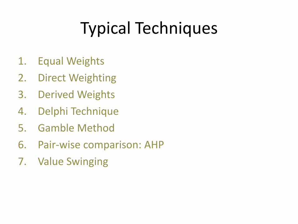
Analytic Hierarchy Process
Select the Best Alternative
Cost Reliability Time Savings
A
B
C
A
B
C
A
B
C
Overall Goal
Criteria
Decision
Alternatives
►Step 1: Structure a hierarchy. Define the problem, determine the criteria and identify the alternatives.
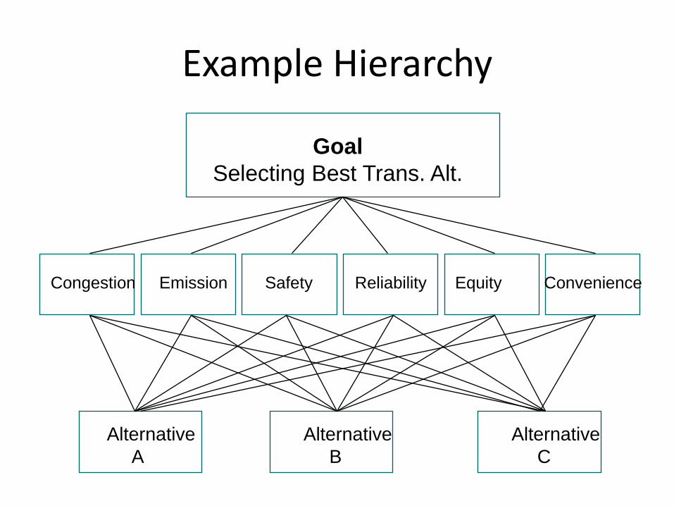
Example Hierarchy
Goal
Selecting Best Trans. Alt.
Congestion Emission Safety Reliability Equity Convenience
Alternative
A
Alternative
C
Alternative
B

AHPExample Problem Statement
• Site selection for a potential traffic generator.
• Three potential sites: – A
– B
– C
• Criteria for site comparisons: – Customer market base.
– Income level
– Infrastructure

AHP Hierarchy Structure
• Top of the hierarchy: the objective (select the best site).
• Second level: how the four criteria contribute to the objective.
• Third level: how each of the three alternatives contributes to each of the four criteria.

AHP General Mathematical Process
• Mathematically determine preferences for sites with respect to each criterion.
• Mathematically determine preferences for criteria (rank order of importance).
• Combine these two sets of preferences to mathematically derive a composite score for each site.
• Select the site with the highest score.
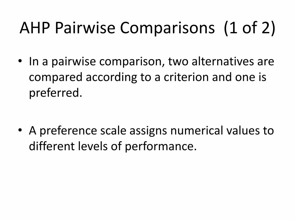
AHP Pairwise Comparisons (1 of 2)
• In a pairwise comparison, two alternatives are compared according to a criterion and one is preferred.
• A preference scale assigns numerical values to different levels of performance.

AHP Pairwise Comparisons (2 of 2)

Example-1 (1) A pairwise comparison matrix summarizes the pairwise
comparisons for a criteria.
Income Level Infrastructure Transportation
A
B
C
193
1/911/6
1/361
11/71
713
11/31
11/42
413
1/21/31
Customer Market
Site A B C
A B C
1 1/3 1/2
3 1 5
2 1/5 1
Example-1 (2)
Customer Market
Site A B C
A B C
1 1/3
1/2 11/6
3 1 5 9
2 1/5 1
16/5
Customer Market
Site A B C
A B C
6/11 2/11 3/11
3/9 1/9 5/9
5/8 1/16 5/16
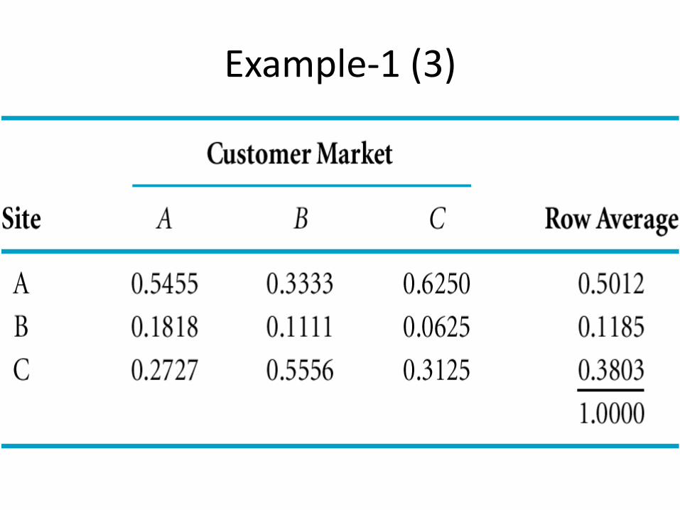
Example-1 (3)

Example-1 (4)
• Preference vectors for other criteria are computed similarly resulting
in the preference matrix

Example-1 (5) Criteria Market Income Infrastructure Transportation
Market Income Infrastructure Transportation
1 5
1/3 1/4
1/5 1
1/9 1/7
3 9 1
1/2
4 7 2 1

Example-1 (6)
Preference Vector for Criteria:
Market
Income
Infrastructure
Transportation
0.0612
0.0860
0.6535
0.1993
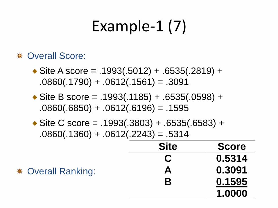
Example-1 (7)
Overall Score:
Site A score = .1993(.5012) + .6535(.2819) +
.0860(.1790) + .0612(.1561) = .3091
Site B score = .1993(.1185) + .6535(.0598) +
.0860(.6850) + .0612(.6196) = .1595
Site C score = .1993(.3803) + .6535(.6583) +
.0860(.1360) + .0612(.2243) = .5314
Overall Ranking:
Site Score
C A B
0.5314 0.3091 0.1595 1.0000

AHP Steps
Develop a pairwise comparison matrix for each decision alternative for each criteria.
Synthesization
Sum the values of each column of the pairwise comparison matrices.
Divide each value in each column by the corresponding column sum.
Average the values in each row of the normalized matrices.
Combine the vectors of preferences for each criterion.
Develop a pairwise comparison matrix for the criteria.
Compute the normalized matrix.
Develop the preference vector.
Compute an overall score for each decision alternative
Rank the decision alternatives.

AHP Consistency
Example: Site selection criteria is how consistent?
Step 1: Multiply the pairwise comparison matrix of the 4 criteria
by its preference vector
Market Income Infrastruc. Transp. Criteria
Market 1 1/5 3 4 0.1993
Income 5 1 9 7 X 0.6535
Infrastructure 1/3 1/9 1 2 0.0860
Transportation 1/4 1/7 1/2 1 0.0612
(1)(.1993)+(1/5)(.6535)+(3)(.0860)+(4)(.0612) = 0.8328
(5)(.1993)+(1)(.6535)+(9)(.0860)+(7)(.0612) = 2.8524
(1/3)(.1993)+(1/9)(.6535)+(1)(.0860)+(2)(.0612) = 0.3474
(1/4)(.1993)+(1/7)(.6535)+(1/2)(.0860)+(1)(.0612) = 0.2473

AHP Consistency
Step 2: Divide each value by the corresponding weight from the
preference vector and compute the average
0.8328/0.1993 = 4.1786
2.8524/0.6535 = 4.3648
0.3474/0.0860 = 4.0401
0.2473/0.0612 = 4.0422
16.257
Average = 16.257/4
= 4.1564
Step 3: Calculate the Consistency Index (CI)
CI = (Average – n)/(n-1), where n is no. of items compared CI = (4.1564-4)/(4-1) = 0.0521 (CI = 0 indicates perfect consistency)

AHP Consistency
N 2 3 4 5 6 7 8 9 10
RI 0 0.58 0.90 1.12 1.24 1.32 1.41 1.45 1.51
Step 4: Compute the Ratio CI/RI
where RI is a random index value obtained from Table below
CI/RI = 0.0521/0.90 = 0.0580
Note: Degree of consistency is satisfactory if CI/RI < 0.10

AHP Decision-Example-2
• Purchasing decision involves, 3 model alternatives, and three decision criteria
• Pairwise comparison matrix
Gear Action
Bike X Y Z
X Y Z
1 3 7
1/3 1 4
1/7 1/4 1
Criteria Price Gears Weight
Price Gears Weight
1 1/3 1/5
3 1
1/2
5 2 1
Weight/Durability
Bike X Y Z
X Y Z
1 1/3 1
3 1 2
1 1/2 1
Price
Bike X Y Z
X Y Z
1 1/3 1/6
3 1
1/2
6 2 1
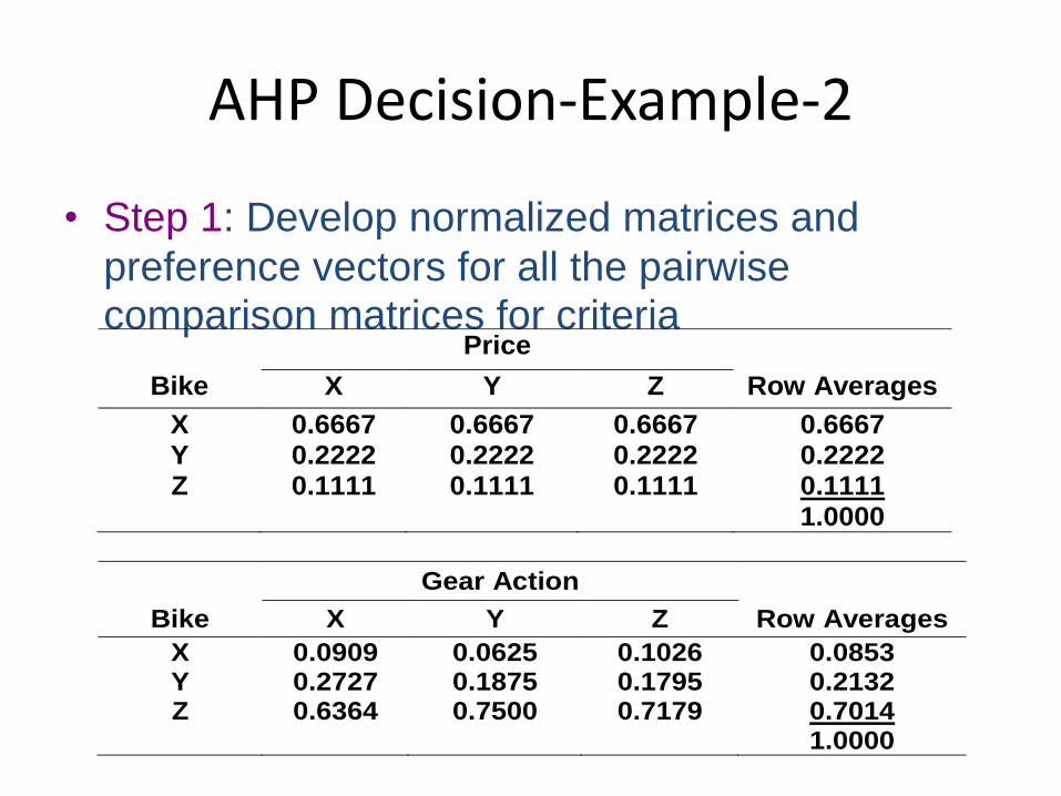
AHP Decision-Example-2
• Step 1: Develop normalized matrices and
preference vectors for all the pairwise comparison matrices for criteria
Price
Bike X Y Z Row Averages
X Y Z
0.6667 0.2222 0.1111
0.6667 0.2222 0.1111
0.6667 0.2222 0.1111
0.6667 0.2222 0.1111 1.0000
Gear Action
Bike X Y Z Row Averages
X Y Z
0.0909 0.2727 0.6364
0.0625 0.1875 0.7500
0.1026 0.1795 0.7179
0.0853 0.2132 0.7014 1.0000

AHP Decision-Example-2
• Step 1 continued: Develop normalized matrices
and preference vectors for all the pairwise
comparison matrices for criteria.
Weight/Durability
Bike X Y Z Row Averages
X Y Z
0.4286 0.1429 0.4286
0.5000 0.1667 0.3333
0.4000 0.2000 0.4000
0.4429 0.1698 0.3873 1.0000
Criteria
Bike Price Gears Weight
X Y Z
0.6667 0.2222 0.1111
0.0853 0.2132 0.7014
0.4429 0.1698 0.3873

AHP Decision-Example-2 Step 2: Rank the criteria.
Price
Gears
Weight
0.1222
0.2299
0.6479
Criteria Price Gears Weight Row Averages
Price Gears Weight
0.6522 0.2174 0.1304
0.6667 0.2222 0.1111
0.6250 0.2500 0.1250
0.6479 0.2299 0.1222 1.0000

AHP Decision-Example-2 Step 3: Develop an overall ranking.
Bike X
Bike Y
Bike Z
Bike X score = .6667(.6479) + .0853(.2299) + .4429(.1222) = .5057
Bike Y score = .2222(.6479) + .2132(.2299) + .1698(.1222) = .2138
Bike Z score = .1111(.6479) + .7014(.2299) + .3873(.1222) = .2806
Overall ranking of bikes: X first followed by Z and Y (sum of
scores equal 1.0000).

Life Cycle Cost Analysis
• A method of calculating the cost of a system over its entire life span.
• It is an engineering economic analysis tool useful in comparing the relative merit of competing project implementation alternatives.
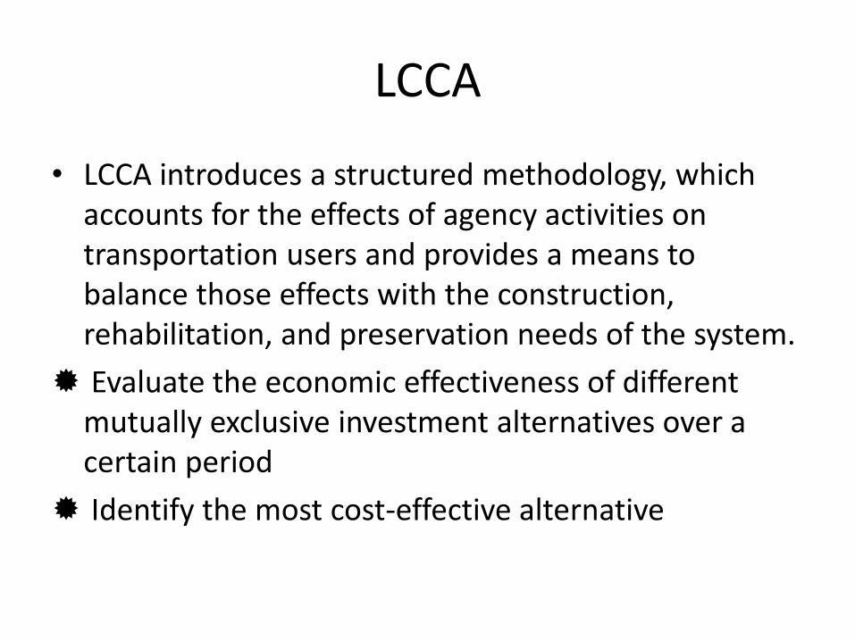
LCCA
• LCCA introduces a structured methodology, which accounts for the effects of agency activities on transportation users and provides a means to balance those effects with the construction, rehabilitation, and preservation needs of the system.
Evaluate the economic effectiveness of different mutually exclusive investment alternatives over a certain period
Identify the most cost-effective alternative

Cost Components of LCCA
32
Since the cost for air quality, noise, etc. are not usually available, it is common practice to include accident costs only.

Life-Cycle Cost Analysis Steps
• Establish design alternatives
• Determine activity timing
• Estimate costs (agency and user)
• Compute life-cycle costs
• Analyze the results
33
Life-Cycle Cost Analysis (LCCA) Steps
• LCCA process begins with the development of alternatives to accomplish the structural and performance objectives for a project.
– A “project” is a transportation improvement that fulfills the agency’s requirements to provide a given level of performance to the public.
– A “project alternative” is a proposed means to provide that performance.
– The economic difference between alternatives is dictated by total cost (when performance is similar).
34
Life-Cycle Cost Analysis (LCCA) Steps
• The analyst then defines the schedule of initial and future activities involved in implementing each project design alternative.
– Note here that the alternatives should have the similar performance levels, otherwise, the project does not fulfill the objective
35

Life-Cycle Cost Analysis (LCCA) Steps
• The costs of these activities are estimated.
– Note that in LCCA, both the agency cost (direct costs like construction and maintenance costs) and user costs (like vehicle operating and running costs) are commonly used.
36
Life-Cycle Cost Analysis (LCCA) Steps
• The predicted schedule of activities and their associated agency and user costs form the projected life-cycle cost stream for each alternative.
• The “discounting” of costs to present worth is performed for cost of the each alternatives.
• An analyst can then determine which one is the most “cost-effective” alternative.
37
Life-Cycle Cost Analysis (LCCA) Steps
• It is to be noted that the most-effective or the lowest cost life-cycle cost option may not necessarily be implemented when other considerations such as risk, available budgets, and political and environmental concerns are taken in to account.
LCCA provides critical information to the overall decision-making process, but not the final answer.
38
LCCA and Benefit-Cost Analysis
• LCCA is a sub-set of benefit-cost analysis
– An agency that uses LCCA has already decided to undertake a project or improvement and is seeking to determine the most cost-effective means to accomplish the project’s objectives.
– LCCA is applied only to compare project implementation alternatives that would yield the same level of service and benefits to the project user at any specific volume of traffic.
39

LCCA and Benefit-Cost Analysis (continued)
– LCCA should consider the costs accrued to the users of the project facility, especially costs associated with increased congestion and reduced safety experienced during project construction and maintenance in addition to the cost
– LCCA does not consider the benefits of an improvement and therefore can not be used to compare design alternatives that do not yield identical benefits.
– Unlike LCCA, benefit-cost analysis can be used to determine whether or not a project should be undertaken at all.
40

LCCA and Benefit-Cost Analysis (continued)
– In Summary, LCCA is a cost-centric approach used to select the most cost-effective alternative that accomplishes a pre-selected project at a specific level of benefits that is assumed to be equal among project alternatives considered.
41
Analysis Period
• A time frame that is sufficiently long to reflect differences in performance among different strategy alternatives.
• It is necessary to select an analysis period over which the alternatives are compared.
• Analysis period (for rehabilitation project) is considered starting at the end of the performance period of the original pavement.

Rehabilitation strategy analysis period beginning at the end of original pavement performance
period 43

Selection of analysis period for alternatives with common performance period, but different performance
44
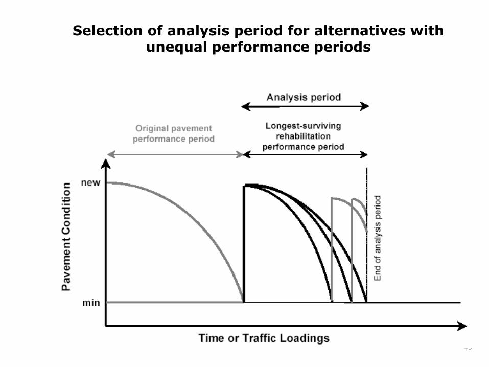
Selection of analysis period for alternatives with unequal performance periods
45

Selection of analysis period to encompass follow-up rehabilitation for all alternatives
46

Discount Rate
• Discount rates used by State DOTs in life cycle cost analysis vary from 0 to 10 percent, with typical values between 3 and 5 percent, and overall average rate of 4 percent.

Monetary Agency Cost
• Costs associated with the alternative that are incurred by the agency during the analysis period, which can be expressed in monetary terms.

User Cost
• Costs associated with the alternative that are incurred by the users of a roadway over the analysis period, which can be expressed in monetary terms.

Categories of User Costs
• Vehicle operating costs - fuel and oil, wear on tires and other parts, registration,
insurance, and others • Delay costs - due to reduced speed and/or use of alternate routes
• Crash costs - damage to the user’s/other vehicles, public/private
property, as well as injuries

Vehicle Operating Cost
In-service vehicle operating costs are a function of pavement serviceability level, which is often difficult to estimate.
Tools are available to model these costs, such as World Bank’s Highway Design and Maintenance Standards Model (HDM-III), FHWA’s Highway Investment Analysis Package (HIAP-Revised), AASHTO Red Book, and others.
Delay Cost
Costs associated with the value of time.
Vary by vehicle class, trip type and trip purpose.
A function of demand for use of the roadway with respect to roadway capacity.
Work zone user delay costs may be significantly different for different rehabilitation alternatives.
Crash Cost
In-service crash rates for different roadway functional classes and crash severities are well known.
Work zone crash rates may differ significantly for different rehabilitation alternatives.

Other Monetary Costs
Those incurred by parties other than the agency or the users of the roadway.
Owners of properties and businesses adjacent to or near the route under study.
Municipalities whose sales tax receipts might be reduced during the period that the nearby businesses were adversely affected.

Salvage Value
The residual value that can be attributed to the alternative at the end of the analysis period.
The value that the item would have in the market place.
Must be defined the same way for all alternatives.
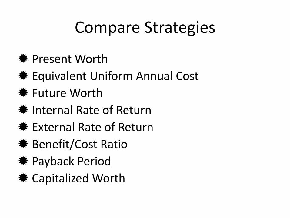
Compare Strategies
Present Worth
Equivalent Uniform Annual Cost
Future Worth
Internal Rate of Return
External Rate of Return
Benefit/Cost Ratio
Payback Period
Capitalized Worth

Sensitivity of Life Cycle Cost Analysis to Key Parameters
• Factors that are more sensitive: • The analysis period and performance period • The predicted traffic over the design and analysis
periods • The initial investment • The discount rate • The timing of follow-up maintenance and
rehabilitation activities • The quantities associated with initial and follow-
up maintenance and rehabilitation
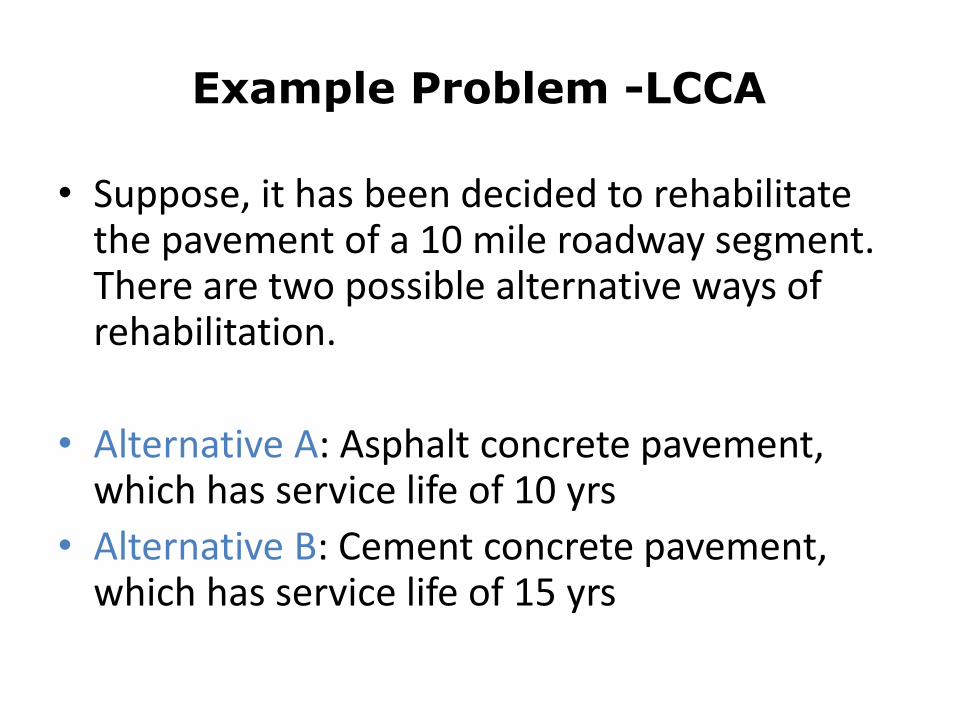
Example Problem -LCCA
• Suppose, it has been decided to rehabilitate the pavement of a 10 mile roadway segment. There are two possible alternative ways of rehabilitation.
• Alternative A: Asphalt concrete pavement, which has service life of 10 yrs
• Alternative B: Cement concrete pavement, which has service life of 15 yrs

Example Problem -LCCA
• You are required to perform “Life Cycle Cost Analysis” for both alternatives.
• Assume, • Interest rate = 7% • Analysis period=30 yrs • The cost components along with the costs are
shown in the following tables • Note that the common that do not vary with the
type of pavement selection are not shown in the cost tables.
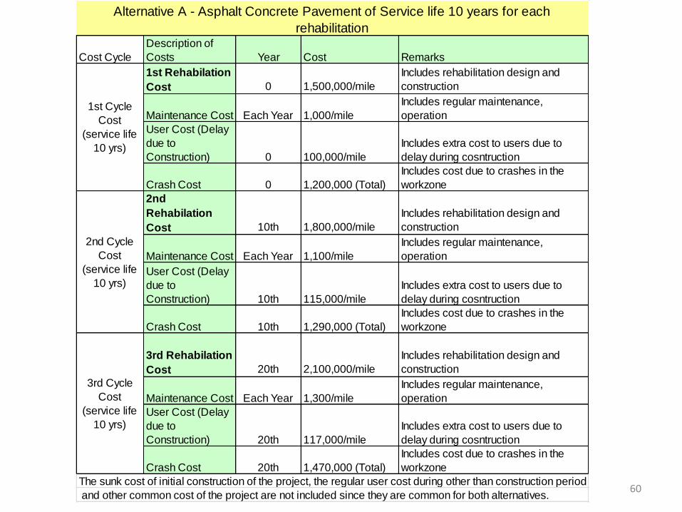
60
Cost Cycle
Description of
Costs Year Cost Remarks
1st Rehabilation
Cost 0 1,500,000/mile
Includes rehabilitation design and
construction
Maintenance Cost Each Year 1,000/mile
Includes regular maintenance,
operation
User Cost (Delay
due to
Construction) 0 100,000/mile
Includes extra cost to users due to
delay during cosntruction
Crash Cost 0 1,200,000 (Total)
Includes cost due to crashes in the
workzone
2nd
Rehabilation
Cost 10th 1,800,000/mile
Includes rehabilitation design and
construction
Maintenance Cost Each Year 1,100/mile
Includes regular maintenance,
operation
User Cost (Delay
due to
Construction) 10th 115,000/mile
Includes extra cost to users due to
delay during cosntruction
Crash Cost 10th 1,290,000 (Total)
Includes cost due to crashes in the
workzone
3rd Rehabilation
Cost 20th 2,100,000/mile
Includes rehabilitation design and
construction
Maintenance Cost Each Year 1,300/mile
Includes regular maintenance,
operation
User Cost (Delay
due to
Construction) 20th 117,000/mile
Includes extra cost to users due to
delay during cosntruction
Crash Cost 20th 1,470,000 (Total)
Includes cost due to crashes in the
workzone
The sunk cost of initial construction of the project, the regular user cost during other than construction period
and other common cost of the project are not included since they are common for both alternatives.
1st Cycle
Cost
(service life
10 yrs)
2nd Cycle
Cost
(service life
10 yrs)
Alternative A - Asphalt Concrete Pavement of Service life 10 years for each
rehabilitation
3rd Cycle
Cost
(service life
10 yrs)

61
Cost Cycle
Description of
Costs Year Cost Remarks
1st Rehabilation
Cost 0 1,700,000/mile
Includes rehabilitation design and
construction
Maintenance Cost Each Year 1,000/mile
Includes regular maintenance,
operation
User Cost (Delay
due to
Construction) 0 100,000/mile
Includes extra cost to users due to
delay during cosntruction
Crash Cost 0 1,400,000 (Total)
Includes cost due to crashes in the
workzone
2nd
Rehabilation
Cost 15th 2,100,000/mile
Includes rehabilitation design and
construction
Maintenance Cost Each Year 1,100/mile
Includes regular maintenance,
operation
User Cost (Delay
due to
Construction) 15th 115,000/mile
Includes extra cost to users due to
delay during cosntruction
Crash Cost 15th 1,570,000 (Total)
Includes cost due to crashes in the
workzone
The sunk cost of initial construction of the project, the regular user cost during other than construction period
and other common cost of the project are not included since they are common for both alternatives.
1st Cycle
Cost
(service life
15 yrs)
2nd Cycle
Cost
(service life
15 yrs)
Alternative B - Cement Concrete Pavement of Service life 15 years for each
rehabilitation

FHWA Software
• http://www.fhwa.dot.gov/infrastructure/asstmgmt/lccasoft.cfm

FHWA LCCA Software

Calculate
Costs (User &
Agency)
Inputs (Traffic Data,
Cost data,
Discount
Rate, etc)
Outputs (NPV curves&
analysis graphs)
Evaluate
Results
in the
Context of
Project
Objectives
Model
traffic
conditions
REALCOST FUNCTIONS Analyst
Function Analyst
Function
FHWA LCCA Software