This is the author’s version of a work that was submitted/accepted for pub-lication in the following source:

He, Jie, Qi, Zhiguo, Hang, Wen, King, Mark J., & Zhao, Chihang (2011)Numerical evaluation of pollutant dispersion at a toll plaza based on sys-tem dynamics and Computational Fluid Dynamics models. TransportationResearch Part C Emerging Technologies, 19(3), pp. 510-520.

This file was downloaded from: http://eprints.qut.edu.au/39776/

c© Copyright 2011 Elsevier Ltd.

Notice: Changes introduced as a result of publishing processes such ascopy-editing and formatting may not be reflected in this document. For adefinitive version of this work, please refer to the published source:

http://dx.doi.org/10.1016/j.trc.2010.08.001

brought to you by COREView metadata, citation and similar papers at core.ac.uk

provided by Queensland University of Technology ePrints Archive

This is the author version published as: This is the accepted version of this article. To be published This is the author version published as: Catalogue from Homo Faber 2007 Abstract B

QUT Digital Repository: http://eprints.qut.edu.au/

He, Jie, Qi, Zhiguo, Hang, Wen, King, Mark J., & Zhao, Chihang (2011) Numerical evaluation of pollutant dispersion at a toll plaza based on system dynamics and Computational Fluid Dynamics models. Transportation Research Part C Emerging Technologies, 19(3), pp. 510-520.

The health of tollbooth workers is seriously threatened by long-term exposure to polluted air from vehicle exhausts. Using traffic data collected at a toll plaza, vehicle movements were simulated by a system dynamics model with different traffic volumes and toll collection procedures. This allowed the average travel time of vehicles to be calculated. A three-dimension Computational Fluid Dynamics (CFD) model was used with a k-ε turbulence model to simulate pollutant dispersion at the toll plaza for different traffic volumes and toll collection procedures. It was shown that pollutant concentration around tollbooths increases as traffic volume increases. Whether traffic volume is low or high (1500 vehicles/h or 2500vehicles/h), pollutant concentration decreases if electronic toll collection (ETC) is adopted. In addition, pollutant concentration around tollbooths decreases as the proportion of ETC-

1

Numerical evaluation of pollutant dispersion at a toll plaza

based on system dynamics and CFD models Jie He1, 2, Zhiguo Qi1, Wen Hang1, Mark King2, Chihang Zhao1

hejie@seu.edu.cn; qzg_001@qq.com; zaeal-hw@sohu.com, mark.king@qut.edu.au, chihangzhao@seu.edu.cn

1 Transportation College, Southeast University, Sipailou 2#, Nanjing City, Jiangsu Province, P.R. China

2 Centre for Accident Research and Road Safety - Queensland (CARRS-Q), Queensland University of Technology

Abstract: The health of tollbooth workers is seriously threatened by long-term exposure to polluted air from vehicle exhausts. Using traffic data collected at a toll plaza, vehicle movements were simulated by a system dynamics model with different traffic volumes and toll collection procedures. This allowed the average travel time of vehicles to be calculated. A three-dimension Computational Fluid Dynamics (CFD) model was used with a k-ε turbulence model to simulate pollutant dispersion at the toll plaza for different traffic volumes and toll collection procedures. It was shown that pollutant concentration around tollbooths increases as traffic volume increases. Whether traffic volume is low or high (1500 vehicles/h or 2500vehicles/h), pollutant concentration decreases if electronic toll collection (ETC) is adopted. In addition, pollutant concentration around tollbooths decreases as the proportion of ETC-equipped vehicles increases. However, if the proportion of ETC-equipped vehicles is very low and the traffic volume is not heavy, then pollutant concentration increases as the number of ETC lanes increases. Keyword: system dynamics; CFD; CO concentration; traffic volume; toll collection method; numerical simulation

Introduction

Toll plazas are important components of highway infrastructure and play an important role in highway operation management. At present, toll plazas in China generally use manual toll collection (MTC) and semi-automatic toll collection (STC). Vehicles spend a long time passing through the toll plaza, including the process of slowing down, stopping to pay the toll and accelerating away from the toll plaza. When traffic is heavy, queues appear prior to the tollbooths. As a result, the health of toll plaza workers is seriously threatened by their exposure to vehicle exhaust emissions. It has been found that the incidence of upper respiratory tract diseases among toll plaza workers is higher than those of other people, due to poor air quality caused by pollution from vehicle exhausts (Huang et al., 2006). Compared to MTC and STC, vehicles can pass through the toll plaza much more quickly without decelerating and stopping when electronic toll collection (ETC) is used. With ETC, the problem of heavy congestion and consequent air pollution caused by vehicle exhausts should be alleviated.

Studies of air pollution at toll plazas have been conducted by undertaking field measurements

(Chen et al.，2007; Diab et al., 2005; Tsai et al., 2002 and 2004; Shih et al., 2008), and analysing

the relationships between pollutant concentrations and various influencing factors such as wind speed, wind direction, temperature, traffic volume, etc. However, field measurement is expensive

2

and time consuming. In addition, there is little opportunity to manipulate the variables being measured, so that it is difficult to distinguish between those variables that are and are not significant contributors to pollutant concentrations (Sagrado et al., 2002). In contrast, numerical simulation offers some advantages compared to field measurements. It is generally less expensive and it provides results of the flow features at every point in space simultaneously (Blocken et al., 2008). Consequently, numerical simulation has become a powerful tool for the researchers.

The CFD (Computational Fluid Dynamics) method is a respected numerical method used to simulate airflow and dispersion and has been widely applied in the field of engineering and environmental studies. The fields of airflow and pollutant concentrations are obtained by solving the equations of momentum, continuity, transport, etc and using appropriate turbulence closure approximation.

Several turbulence models including the standard k-ε model (Jones and Launder, 1972), the RNG k-ε model (Yakhot and Orszag, 1986 and 1988), the realizable k-ε model (Shih et al., 1995), the Reynolds Stress model (Launder et al., 1975), Large Eddy Simulation (LES) (Ghosal et al., 1995), etc. have been used in solving various problems in CFD simulation of pollutant dispersion, and comparisons between numerical simulation and wind tunnel results have been favourable.

A two-dimensional numerical model based on Reynolds-averaged Navier–Stokes (RANS)

equations coupled with a series of standard, Renormalisation Group (RNG) and realizable k-ε turbulence models was developed by Chan et al.(2002) to simulate fluid flow development and pollutant dispersion within an isolated street canyon. Among the studied turbulence models, the RNG k-ε turbulence model was found to be the optimum turbulence model when the results of modelling were compared with wind tunnel tests. Sagrado et al. (2002) studied pollutant dispersion in a two-dimensional street canyon using the realizable k-ε model, with the principal parameter investigated being the height of the downstream building. Two-dimensional LES numerical simulation was conducted by Laatar et al. (2002) to investigate the effect of wind on covered roads. Huang et al. (2008) carried out a three-dimensional CFD simulation coupled with the standard k-ε model to analyse the pollutant dispersion under non-isothermal conditions within small defined area in Kawasaki city, Japan, in winter. The temporal variations of wind speed and pollutant concentrations were analyzed at the pedestrian level (1.5m above the ground level).

Among the existing CFD approaches, the RANS approach has been widely used for flow and dispersion calculations in complex environments. This approach offers significant predictive advantages compared to other simpler approaches, when the geometrical layout is complex (Venetsanos et al., 2000). On the other hand other more accurate CFD approaches like LES or DNS (Direct Numerical Simulation) are restricted by computational power as the Reynolds numbers they use are generally much lower than the typical environmental applications.

However, the CFD method has some disadvantages. For example, the computational domain must not be too large because of the limitations of computer hardware. Furthermore, CFD simulation needs an extensive field data base so that some of the parameters can be calibrated.

In this paper, using actual traffic data, a simulation model based on the system dynamics was established to investigate the effects of traffic volume, number and configuration of ETC lanes, and proportion of ETC-equipped vehicles on the average travel time for all vehicles passing through a toll plaza. Using this information, pollutant emission levels were calculated and several three-dimension CFD simulations of pollutant dispersion at the toll plaza were conducted using

3

the commercial computer program FLUENT. The fields of velocity flow and pollutant concentration were simulated and the effects of traffic volume and toll collection procedures on pollutant dispersion were discussed.

1 Traffic simulation at the toll plaza

In this section, movements of vehicles at the toll plaza were simulated by using a system dynamics model. The average travel time for all vehicles passing through the toll plaza was calculated, and hence the levels of vehicle emitted pollutant were determined.

1.1 Model description and setup

System dynamics is a method for studying the complex behaviour of dynamic systems. It describes the structure of the system and simulates system dynamic behaviour using the control principles of information feedback and logical analysis of causality (Forrester, 1992). System dynamics can be utilised for system problems with dynamic feedback, and its theories have been applied to many fields including industrial processes, economics, ecology, environmental studies, etc (Gertseva et al, 2004; Higgins et al, 1997; Cheng et al, 2007). Universal simulation platforms for system dynamics include Vensim, Stella, Powersim and so on. A toll plaza is a complicated system in which the vehicles’ travel conditions are influenced by many factors that interact with each other and co-determine the toll plaza operation’s efficiency. Hence, it is appropriate to simulate vehicle travel characteristics at a toll plaza utilising system dynamics.

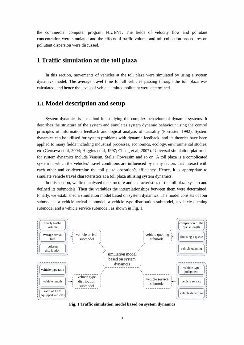
In this section, we first analyzed the structure and characteristics of the toll plaza system and defined its submodels. Then the variables the interrelationships between them were determined. Finally, we established a simulation model based on system dynamics. The model consists of four submodels: a vehicle arrival submodel, a vehicle type distribution submodel, a vehicle queuing submodel and a vehicle service submodel, as shown in Fig. 1.

hourly traffic volume

average arrival rate

poisson distribution

vehicle type ratio

vehicle length

ratio of ETC equipped vehicles

vehicle arrival submodel

vehicle type distribution submodel

simulation model based on system

dynamcis

vehicle queuing submodel

vehicle service submodel

comparison of the queue length

choosing a queue

vehicle queuing

vehicle type judegment

vehicle service

vehicle departure

Fig. 1 Traffic simulation model based on system dynamics

4

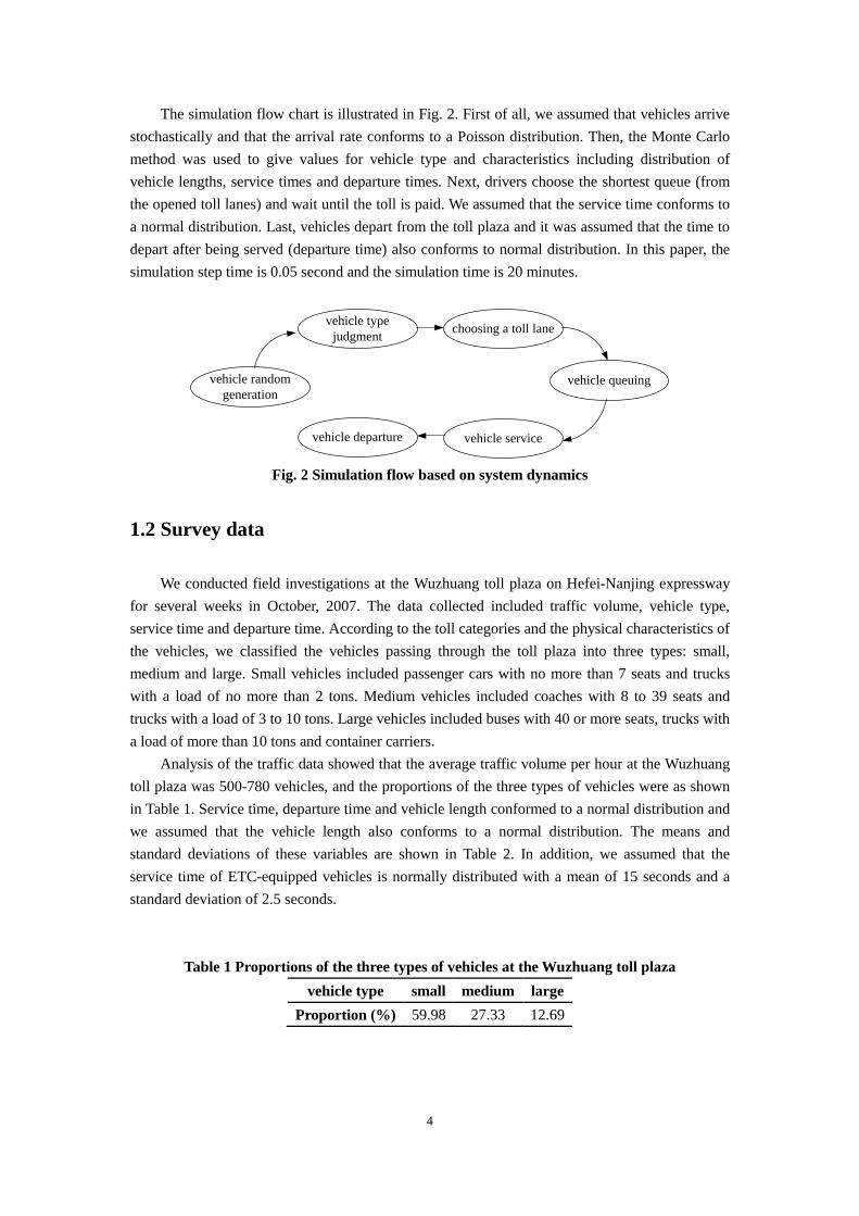
The simulation flow chart is illustrated in Fig. 2. First of all, we assumed that vehicles arrive stochastically and that the arrival rate conforms to a Poisson distribution. Then, the Monte Carlo method was used to give values for vehicle type and characteristics including distribution of vehicle lengths, service times and departure times. Next, drivers choose the shortest queue (from the opened toll lanes) and wait until the toll is paid. We assumed that the service time conforms to a normal distribution. Last, vehicles depart from the toll plaza and it was assumed that the time to depart after being served (departure time) also conforms to normal distribution. In this paper, the simulation step time is 0.05 second and the simulation time is 20 minutes.

vehicle random generation

vehicle type judgment choosing a toll lane

vehicle queuing

vehicle servicevehicle departure

Fig. 2 Simulation flow based on system dynamics

1.2 Survey data

We conducted field investigations at the Wuzhuang toll plaza on Hefei-Nanjing expressway for several weeks in October, 2007. The data collected included traffic volume, vehicle type, service time and departure time. According to the toll categories and the physical characteristics of the vehicles, we classified the vehicles passing through the toll plaza into three types: small, medium and large. Small vehicles included passenger cars with no more than 7 seats and trucks with a load of no more than 2 tons. Medium vehicles included coaches with 8 to 39 seats and trucks with a load of 3 to 10 tons. Large vehicles included buses with 40 or more seats, trucks with a load of more than 10 tons and container carriers.

Analysis of the traffic data showed that the average traffic volume per hour at the Wuzhuang toll plaza was 500-780 vehicles, and the proportions of the three types of vehicles were as shown in Table 1. Service time, departure time and vehicle length conformed to a normal distribution and we assumed that the vehicle length also conforms to a normal distribution. The means and standard deviations of these variables are shown in Table 2. In addition, we assumed that the service time of ETC-equipped vehicles is normally distributed with a mean of 15 seconds and a standard deviation of 2.5 seconds.

Table 1 Proportions of the three types of vehicles at the Wuzhuang toll plaza vehicle type small medium large

Proportion (%) 59.98 27.33 12.69

5

Table 2 Service time, departure time and vehicle length vehicle type small medium large

service time mean value (s) 22.4 28.87 34.59

standard deviation 8.73 9.15 11.75

departure time mean value (s) 9.02 17.31 30.10

standard deviation 8.22 9.79 13.25

vehicle length mean value (m) 6 10 16

standard deviation 1 3 3

1.3 Simulation results

In order to study the effects of traffic volume and toll collection method on pollutant dispersion at a toll plaza, we designed a simulation scheme as shown in Table 3. STC is used at the Wuzhuang toll plaza currently and partial ETC lanes will be built in the near future. We considered two toll collection procedures: the current STC method and mixed toll collection with STC and ETC. In the mixed toll collection method, two cases with two ETC lanes and four ETC lanes were considered separately, using the same total of 20 open toll lanes in all cases. In each case, we simulated two proportions of ETC-equipped vehicles and two traffic volumes. In the STC arrangement, we simulated five traffic volumes from 500 vehicles per hour to 2500 vehicles per hour.

Table 3 Simulation scheme traffic volume (vehicles/h) ETC lanes proportion of ETC-equipped

vehicles (%) 1

500、1000、1500、2000、2500 0 0

2 1500、2500

2 10

3 1500、2500

2 20

4 1500、2500

4 10

5 1500、2500

4 20

In accordance with the above simulation scheme, simulations were conducted and the results

were obtained as shown in Fig. 3. Fig. 3 (a) illustrates the average travel time for all vehicles for the five traffic volumes. The average travel times for the cases with 2 ETC lanes and 4 ETC lanes are shown in Fig. 3(b) and (c), respectively. From Fig. 3 (a) we can see that the average travel time for all vehicles increases as the traffic volume increases. From Fig. 3 (b) and (c) we can see that the average travel time increases as the traffic volume increases no matter how many the ETC lanes are available. For the same traffic volume, the average travel time decreases as the proportion of ETC-equipped vehicles increases.

6

The simulation results for STC and the mixed ETC/STC methods with the same traffic volume are compared in Table 4. In the column for mixed toll collection, the first number shown is for the results when the proportion of ETC-equipped vehicles is 10%, while the numbers in brackets show the simulation results when the proportion is 20%.

From Table 4 we can see that the average travel time is the shortest when there are two ETC lanes and the average travel time becomes shorter as the proportion of ETC equipped vehicles increases from 10% to 20%. If the proportion of ETC-equipped vehicles is 10%, average travel time is the shortest when there are two ETC lanes rather than four. This is because four ETC lanes are underutilized and the travel time of vehicles which are not ETC-equipped is extended because there are less STC lanes provided. As a result, in the 10% case travel times are lowest for the two ETC lane case (though not by much for a volume of 1500 vehicles per hour) and highest for the four ETC case, especially when the volume is 2500 vehicles per hour, while the STC case lies between. When the proportion of ETC-equipped vehicles increases to 20%, this picture changes. The two ETC lane case continues to provide the shortest travel times, but the four ETC case also provides substantially shorter travel times (especially at 2500 vehicles per hour) than the STC case. At this higher proportion of ETC-equipped vehicles, the utilization of ETC lanes is increased and the capacity of the toll plaza is improved. However, having 20% of the toll plaza with ETC lanes (four of the 20 lanes) does not provide greater efficiency where 20% of vehicles are ETC-equipped because their shorter travel times mean that the four ETC lanes are relatively under-utilized (and the 16 STC lanes over-utilized) compared with the full STC case. This demonstrates that when the proportion of ETC-equipped vehicle is low, less rather than more ETC lanes can better improve the overall capacity of the toll plaza.

(a) Average travel time of five traffic volumes

(b) Average travel time with 2 ETC lanes (c) Average travel time with 4 ETC lanes

7

Fig. 3 Simulation results of the system dynamics model

Table 4 Average travel time under two collection manners (unit: second) traffic volume semi-automatic

toll collection mixed toll collection for ETC-

equipped proportion 10% (20%) STC only 2 ETC lanes 4 ETC lanes

1500 vehicles/h 38.77 38.44(33.04) 42.75(34.89) 2500 vehicles/h 192.80 181.01(72.20) 246.13(115.09)

2 CFD modelling

2.1 Toll plaza dimensions

The Wuzhuang toll station is located on the Hefei-Nanjing highway with 22 toll lanes as shown in Fig. 4. There are 11 lanes in each direction, and two lanes for entering and leaving the toll plaza area. The distance between the two sides of the toll plaza is about 120m. The toll canopy

is 10m above the ground, with dimensions of 120m×20m×1m. The widths of toll lanes,

super-wide lanes and shoulders are 3.2m, 4.0m and 0.75m, respectively. Fig. 5 shows the layout of the Wuzhuang toll plaza in one direction.

Fig.4. Photo of the Wuzhuang Toll Station

TOLL

CANOPY

8

Fig. 5 Schematic diagram of the toll plaza, one direction only (11 lanes)

2.2 CFD model of the toll plaza

A simplified three-dimension CFD model of the toll plaza was designed based on the actual physical dimensions as shown in Fig. 6. The origin of the coordinates is the centre of the bottom face of the middle tollbooth. The x axis and y axis are parallel and perpendicular to the traffic

direction respectively. A tollbooth is simplified as a cube with the dimensions 2.5m×1.5m×2.4m.

The inlet and the lateral and top boundaries are 5H away from the tollbooth, where H is the height of the toll canopy (i.e. 5H is 50m). The outflow boundary is positioned at least 20H (200m) behind the tollbooth (Franke et al., 2004). Therefore, the dimensions of the computational domain

are 310m×220m×60 m.

Fig. 6 Illustration of the computational domain

Calculations were performed with an unstructured grid generation, and the computational domain was built using tetrahedral cells with a finer resolution close to the ground (He et al., 2009). The computational domain was split into ten layers horizontally. The bottom part which was attached to the ground was meshed with a grid size of 1m. As the height increased, the grid size of each layer became bigger with a ratio of 1.2. In this way, mesh quality was ensured and calculation speed was improved. The convergence criterion for each variable was 1×10-6.

3 Boundary conditions

3.1 Calculation of pollutant source strength

The pollutant source within the toll plazas is vehicle-emitted exhaust gases which are composed of CO, HC, NOx and so on. Because CO is relatively stable in the air, we choose it as

9

the representative pollutant to analyze the pollutant dispersion in the vicinity of tollbooths. CO, which results from the incomplete combustion of fossil fuel, is one of the major pollutants emitted by motor vehicles. It is of interest because of its significant health effects, due to haemoglobin binding more effectively (245 times more) with CO than with O2 (Diab et al, 2005). Effects range from headaches, dizziness, lassitude and vision problems at low doses to nausea, vomiting, muscle weakness and difficulty in breathing at moderate to high doses, and unconsciousness and death resulting from chronic exposure.

Pollutant sources are typically modelled either as points (Chang and Meroney, 2003) or lines (Chang and Meroney, 2001; Sagrado et al., 2002; Chan et al., 2002). In this paper, the pollutant

source was modelled as lines placed in the middle of each lane with dimensions of 100m×0.2m

based on the distance vehicles travel within the toll plaza. The pollutant source strength can be calculated as follows:

13600

n

i ii

tQ K AS =

=• ∑

In the above formula, Q represents the emission strength of vehicle-induced pollutants (kg/(m2·s));

Ki represents the single vehicle emission factor (kg/s) of vehicle type i, i=1, 2 … n; Ai represents the traffic density (vehicles/h) of vehicle type i; t represents the time spent by vehicles passing through the toll plaza; S represents the area of the pollutant source.

3.2 Settings of other boundary conditions

A velocity inlet boundary condition was used for inlet wind flow with wind direction parallel to the x axis. Because the toll plaza is in the atmospheric boundary layer near the ground, incoming wind velocity u at height z above the ground has an atmospheric boundary layer profile

( )1/7' / 'zu u z z= (Nazridoust and Ahmadi, 2006) where 'zu is the wind speed at a reference

height of 'z which is equal to 60 m in this case. The local meteorology monitoring station confirmed that the dominant wind direction was perpendicular to the tollbooths . For the outlets at the end of the domain, an outflow boundary condition was assumed. The top and lateral surfaces of the domain were treated as three planes of symmetry. All other solid surfaces of the domain (surfaces of tollbooths, toll canopy and retaining walls) were defined as walls with no slip velocity boundary condition. On the walls, conditions of zero diffusive flux and stick-upon-impact for gaseous pollutants were imposed. The line sources of CO were treated as mass flow inlets.

4 Results and discussions

The Chinese national standard Ambient Air Quality Standard (GB3095-1996) divides the country into three class areas in terms of land use, two which it applies two standards of air quality. First class areas include nature reserves, scenic spots and other areas that need to be protected. Second class areas include residential districts, mixed business and residential areas, areas of

10

cultural interest, ordinary industrial estates and rural areas. Third class areas are special industrial estates. Air quality standards for the three class areas in terms of CO concentration limits are specified in Table 5.

Table 5 Limit values for CO concentration in the Ambient Air Quality Standard

land use classes

concentration unit first class second class third class

daily average 4.00 4.00 6.00 mg/m3

hourly average 10.00 10.00 20.00 The CFD simulation results presented in this section are compared with these limits. We

chose the 1.5m height plane as the observation surface, because it is the breathing height of the toll collectors. We also determined CO concentrations on three lines: the central line of the computational domain perpendicular to the X axis (x=0m) and the two lines five metres before (x=-5m) and after (x=5m) it.

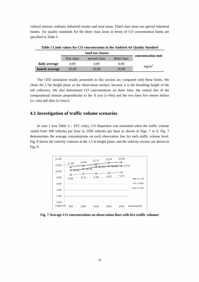
4.1 Investigation of traffic volume scenarios

In case 1 (see Table 3 – STC only), CO dispersion was simulated when the traffic volume varied from 500 vehicles per hour to 2500 vehicles per hour as shown in Figs. 7 to 9. Fig. 7 demonstrates the average concentrations on each observation line for each traffic volume level. Fig. 8 shows the velocity contours at the 1.5 m height plane, and the velocity vectors are shown in Fig. 9.

Fig. 7 Average CO concentrations on observation lines with five traffic volumes

11

Fig. 8 Velocity contour at the 1.5 m height plane

From Fig. 8 we can see that wind speed behind and around the tollbooths is lower than that in

the windward direction because of the obstruction of the tollbooths. The expanded section in Fig. 8 shows that wind speed in the spaces between the tollbooths is greater than that around the tollbooths. There are also some “micelles” apparent in Fig. 8, areas where the speed is lower than the surroundings without there being any physical barriers, which is a result of turbulence.

Fig. 9 Vectors of velocity around a tollbooth at the 1.5 m height plane

In Fig. 7, average CO concentration lie within the range of 8.86 to12.99 mg/m3. On the

observation lines 5 meters before and after the booth, but at the same height, the average CO concentration becomes higher as the traffic volume increases. The lowest CO concentrations appear on the central line of the computational domain (x=0 m), the concentrations on the windward line (x=-5 m) are higher, and the highest concentrations appear on the line behind the tollbooths (x=5 m). Looking at the wind speed distribution in Fig. 8 and vectors of velocity in Fig. 9, we can see that wind speed is much lower behind the tollbooth and backflow appears. This explains why the CO concentration value behind the tollbooth was higher than the values at or before the tollbooth. This demonstrates that wind speed and airflow pattern have a considerable

12

effect on the dispersion of pollutants around the tollbooths. Comparing the CO concentrations in these simulation results with the limit values in Table 5,

we can see that the CO concentrations on the line of x=0m (the tollbooth) are lower than the hourly (but not the daily) average limits for all land use areas, while the CO concentrations on the other two lines (before and after the tollbooth) are only lower than the average hourly limit for third class areas.

4.2 Investigation of toll collection scenarios

For cases 2 to 5 (the mixed toll collection cases with two or four lanes and 10% or 20% of ETC-equipped vehicles), the CO concentration on the observation line (x=0m) was calculated and the simulation results are shown in Fig. 10 with traffic volumes of 1500 vehicles/h and 2500 vehicles/h.

As Fig. 10 shows, with the same traffic volume and proportion of ETC-equipped vehicles, the average CO concentration on the observation line is the lowest when there are two ETC lanes. When there are 4 ETC lanes at the lower traffic volume of 1500 vehicles/h, the average CO concentration on the observation line is about the same as when only STC is used, and there is a clear advantage to having two ETC lanes in terms of CO concentrations. Overall, CO concentrations are lower at this lower traffic volume because travel times are lower (see Table 4). However, when there are four rather than two ETC lanes, the ETC lanes are underutilized because of low proportion of ETC equipped vehicles. Consequently, the average travel time for the non-ETC equipped vehicles is extended and the average concentrations of pollutants are higher than those with two ETC lanes.

When the traffic volume is 2500 vehicles/h, the average CO concentrations with two ETC lanes and four ETC lanes are very similar, and both are lower than those for STC alone. This shows that increasing the number of ETC lanes facilitates pollutant dispersion and decreases pollutant concentration when traffic is heavy.

It can also be seen, for both levels of traffic volume and both the two and four lane ETC cases, that the CO concentration decreases when the proportion of ETC-equipped vehicles increases.

13

Fig. 10 Simulation results of cases 2-5 (T represents traffic volume, R represents the proportion of ETC equipped vehicles, STC means semi-automatic toll collection, MTC means a mixed toll collection with STC and ETC)

5 Conclusions

The effects of traffic volume and toll collection method on pollutant dispersion at a highway toll plaza were studied in this paper. By comparing the simulation results, some conclusions are summarised as follows.

Pollutant concentration increases as traffic volume increases. When the mixed toll collection with ETC lanes is adopted, pollutant concentration is lower than when only STC is used. In addition, pollutant concentration decreases as the proportion of ETC-equipped vehicles rises. For the same proportion of ETC-equipped vehicles and when the traffic volume is not heavy, pollutant concentration increases as the number of ETC lanes is increased, because too many ETC lanes when there is a low proportion of ETC-equipped vehicles increases the average travel time for the non-ETC equipped vehicles, leading to a build-up of pollutant concentration to about the same level as the STC only case. However, when traffic volume is heavy, the advantage of ETC lanes is apparent and the pollutant concentration becomes lower than with STC, and does not vary appreciably as the number of ETC lanes increases from two to four, even though travel time modelling (see Table 4) shows a marked increase in average travel times in this condition due to the relative under-utilization of the ETC lanes. This means that increases in travel times do not necessarily translate into higher levels of pollutant dispersion, which has an important policy implication: introducing more ETC lanes than is optimal in terms of travel time does not necessarily lead to additional adverse pollution outcomes, and therefore can prepare for growth in the proportion of ETC-equipped vehicles.

Due to the logistical constraints on collecting comprehensive field measurement data, we focused on the qualitative analysis of simulation results. In addition, simulation offers a greater facility to model and explain the instantaneous circumstances than field measurements because of the inability to control all the environmental variables in the field. However, field measurements

14

under different conditions are still important, as they are needed to further validate the simulation results.

One of the main issues which stimulated this research was concern about the health of tollbooth workers. The modelling of CO concentrations under the various scenarios in this study shows that the concentration of CO at the tollbooth itself lies just under the 10 mg/m3 hourly limit set out in the Chinese Ambient Air Quality Standard (GB3095-1996) for first and second class areas, and well below the 20 mg/m3 limit for third class areas. However, tollbooth workers may be at work for long hours, and the daily average limits are much lower, at 4 mg/m3 for first and second class areas, and 6 mg/m3 for third class areas. As an example, a tollbooth work who works for 8 hours will be exposed to about 80 mg/m3 in that period, so that exposure to a further 16 mg/m3 over the other 16 hours (i.e. only 1 mg/m3 per hour) would cause them to exceed the daily limits for first class and second class areas. As emission control regulations are introduced gradually, the emission volume of vehicles will decrease and air quality will be improved to a certain extent, however the simulation results in this paper indicate that levels are currently high enough to warrant concern. It is suggested that a source of clean air from an area remote from the plaza should be provided in booth ventilation system.

6 Acknowledgements

The authors would like to thank Southeast University for its financial support (project “Southeast excellent young staff foundation 2008-2011”), Xu Jiabing (Anhui Province Communications Department) for providing essential data and support and Professor Rod Troutbeck (Centre for Accident Research and Road Safety - Queensland (CARRS-Q), Queensland University of Technology) for grammar edit.

References

Blocken, B., Stathopoulos, T., Saathoff, P., Wang, X. 2008. Numerical evaluation of pollutant dispersion in the built environment: Comparisons between models and experiments. Journal of Wind Engineering and Industrial Aerodynamics 96, 1817-1831. Chan, T.L., Dong, G., Leung, C.W., Cheung, C.S., Hung, W.T., 2002. Validation of a two-dimensional pollutant dispersion model in an isolated street canyon. Atmospheric Environment 36, 861-872. Chang, C.H., Meroney, R.N., 2001. Numerical and physical modeling of bluff body flow and dispersion in urban street canyons. Journal of Wind Engineering and Industrial Aerodynamics 89, 1325-1334. Chang, C.H., Meroney, R.N., 2003. Concentration and flow distributions in urban street canyons: wind tunnel and computational data. Journal of Wind Engineering and Industrial Aerodynamics 91, 1141-1154. Chen, K.J., Chen, K.L., Zhang, L.J., Leng, G.Y., 2007. Characteristics and influencing factors of air pollution in and out of the highway toll gates. Environmental Science 28, 1847-1853. Cheng, H.S., Wang, Y., Li, S.S. Sun., R.Y., 2007. Applications of system dynamics software STELLA in ecology. Journal of South China Normal University (Natural science edition) 3,

15

126-131. Diab, R.D., Foster, S.J., François, K., Martincigh, B.S., Salter, L.F., 2005. Carbon monoxide levels at a toll plaza near Durban, South Africa. Environmental Chemistry Letters 3, 91-84. Forrester, J.W., 1992. From the ranch to system dynamics: An autobiography. BEDEIAN A G. Management Laureates: A Collection of Autobiographical Essays. Greenwich: JAI Press, 343-369. Franke, J., Hirsch, C., Jensen, A.G., Krüs, H.W., Schatzmann, M., Westbury, P.S., Miles, S.D., Wisse, J.A., Wright, N.G., 2004. Recommendations for CFD in wind engineering. In: Proceedings of the International Conference on Urban Wind Engineering and Building Aerodynamics. In: van Beeck JPAJ (Ed.), COST Action C14, Impact of Wind and Storm on City Life Built Environment. von Karman Institute, Sint-Genesius-Rode, Belgium, 5-7. Gertseva, V.V., Schindler, J.E., Gertsev V.I., Ponomarev, N.Y., English, W.R., 2004. A simulation model of the dynamics of aquatic macroinvertebrate communities. Ecological Modelling 176, 173-186. Ghosal, S., Lund, T.S., Moin, P., Akselvoll, K., 1995. A dynamic localization model for large-eddy simulation of turbulent flows. Journal of Fluid Mechanics 286, 229-255, Cambridge University Press, U.K. He, J., Qi, Z., Zhao, C., Bao, X., 2009. Simulations of pollutant dispersion at toll plazas using

three-dimensional CFD models. Transportation Research Part D 14, 557–566.

Higgins, S.I., Turpie, J.K., Costanza, R., Cowling, R.M., Le Maitre, D.C., Marais, C., Midgley, G.F., 1997. An ecological economic simulation model of mountain fynbos ecosystems: Dynamics, valuation and management. Ecological Economics 22, 141-156. Huang, Z.N., Pan, J.C., Wu, Y.J., Huang, C.Y., 2006. Investigation on health effect of indoor air pollution in the toll-gates. Occupational Health and Emergency Rescue 24, 43-44. Huang, H., Ooka, R., Chen, H., Kato, S., Takahashi, T., Watanabe, T., 2008. CFD analysis on traffic-induced air pollutant dispersion under non-isothermal condition in a complex urban area in winter. Journal of Wind Engineering and Industrial Aerodynamics 96, 1774-1788. Jones, W.P., Launder, B.E., 1972. The prediction of laminarization with a 2-equation model of turbulence. International Journal of Heat and Mass Transfer 15, 301. Laatar, A.H, Benahmed, M., Belghith, A, Le Quéré, P., 2002. 2D large eddy simulation of pollutant dispersion around a covered roadway. Journal of Wind Engineering and Industrial

Aerodynamics 906, 17–637.

Launder, B.E., Reece, G.J., Rodi, W., 1975. Progress in the development of a Reynolds-stress

turbulence closure. Journal of Fluid Mechanics 68, 537–566.

Nazridoust, K., Ahmadi, G., 2006. Airflow and pollutant transport in street canyons. Journal of Wind Engineering and Industrial Aerodynamics 94, 491-522. Neofytou, P., Venetsanos, A.G., Rafailidis, S., Bartzis, J.G., 2006. Numerical investigation of the pollution dispersion in an urban street canyon. Environmental Modelling & Software 21, 525-531. Sabatino, S.D., Buccolieri, R., Pulvirenti, B., Britter, R., 2007. Simulations of pollutant dispersion within idealised urban-type geometries with CFD and integral models. Atmospheric Environment 41, 8316-8329. Sagrado, A.P.G., Beeck, J.V., Rambaud, P., Olivari, D., 2002. Numerical and experimental

16

modelling of pollutant dispersion in a street canyon. Journal of Wind Engineering and Industrial Aerodynamics 90, 321-339. Shih, T.H., Liou, W.W., Shabbir, A., Yang Z., Zhu, J., 1995. A new k–ε eddy-viscosity model for high Reynolds number turbulent flows+model development and validation. Computers & Fluids

24, 227–238.

Shin, T.S., Lai, C.H., Hung, H.F., Ku, S.Y., Tsai, P.J., Yang, T., Liou, S.H., Loh, C.H., 2008. Elemental and organic carbon exposure in highway tollbooths: A study of Taiwanese toll station workers. Science of the Total Environment 402, 163-170. Tsai, P.J., Lee C.C., Chen M.R, Shih, T.S., Lai, C.H., Liou, S.H., 2002. Predicting the contents of BTEX and MTBE for the three types of tollbooth at a highway toll station via the direct and indirect approaches. Atmospheric Environment 36, 5961-5969 Tsai, P.J., Shih, T.S., Chen, H.L., Lee, W.J., Lai, C.H., Liou, S.H., 2004. Assessing and predicting the exposures of polycyclic aromatic hydrocarbons (PAHs) and their carcinogenic potencies from vehicle engine exhausts to highway toll station workers. Atmospheric Environment 38, 333-343 Venetsanos, A.G., Bartzis, J.G., Würtz, J., Papailiou, D.D., 2000. Comparative modeling of a passive release from an L-shaped building using one, two and three-dimensional dispersion

models. International Journal of Environment and Pollution 14, 324–333.

Yakhot, V., Orszag, S.A., 1986. Renormalization group analysis of turbulence. I. Basic theory, Journal of Science Computing 1, 3-51. Yakhot, V., Orszag, S.A., 1988. Computational test of the renormalization group theory of turbulence, Journal of Science Computing 3, 139-147.