Transport link scanner: simulating geographic transport · PDF filetransport network expansion...

ORIGINAL ARTICLE

Transport link scanner: simulating geographictransport network expansion through individualinvestments

C. Jacobs-Crisioni1 • C. C. Koopmans2

Received: 27 July 2015 / Accepted: 19 May 2016 / Published online: 10 June 2016

� The Author(s) 2016. This article is published with open access at Springerlink.com

Abstract This paper introduces a GIS-based model that simulates the geographic

expansion of transport networks by several decision-makers with varying objec-

tives. The model progressively adds extensions to a growing network by choosing

the most attractive investments from a limited choice set. Attractiveness is defined

as a function of variables in which revenue and broader societal benefits may play a

role and can be based on empirically underpinned parameters that may differ

according to private or public interests. The choice set is selected from an

exhaustive set of links and presumably contains those investment options that best

meet private operator’s objectives by balancing the revenues of additional fare

against construction costs. The investment options consist of geographically plau-

sible routes with potential detours. These routes are generated using a fine-meshed

regularly latticed network and shortest path finding methods. Additionally, two

indicators of the geographic accuracy of the simulated networks are introduced. A

historical case study is presented to demonstrate the model’s first results. These

results show that the modelled networks reproduce relevant results of the histori-

cally built network with reasonable accuracy.

Keywords Transportation � Network growth � Agent-based modelling

& C. Jacobs-Crisioni

[email protected]

C. C. Koopmans

[email protected]

1 Institute for Environment and Sustainability, Sustainability Assessment Unit, European

Commission, Joint Research Centre, Via E. Fermi, 2749, 21027 Ispra, VA, Italy

2 Faculty of Economics and Business Administration, VU University Amsterdam, Boelelaan

1105, 1081 HV Amsterdam, The Netherlands

123

J Geogr Syst (2016) 18:265–301

DOI 10.1007/s10109-016-0233-y

http://crossmark.crossref.org/dialog/?doi=10.1007/s10109-016-0233-y&domain=pdf

http://crossmark.crossref.org/dialog/?doi=10.1007/s10109-016-0233-y&domain=pdf

JEL Classification H54 � L92 � O33 � R42

1 Introduction

The expansion of transport networks is considered an important factor for the spatial

distribution of activities and receives considerable politic and academic attention. It

is commonly perceived as a technology diffusion process in which the innovation

spreads geographically (Grubler 1990; Nakicenovic 1995). The geographic paths

that the developed networks assume have important societal and economic

ramifications. Ideally these paths constitute a social optimum considering

construction costs and generalized travel costs. However, due to often non-

cooperative decision-makers (Knick Harley 1982; Dobbin and Dowd 1997; Xie and

Levinson 2011), potential transport network expansion outcomes may be limited to

Nash equilibria (Bala and Goyal 2000; Anshelevich et al. 2003) that can entail

considerable extra costs to reach a target state of connectivity.

Although it is known that transport network expansion may follow a clear

rationale, largely based on, e.g. expected transport flows versus costs (Rietveld and

Bruinsma 1998; Xie and Levinson 2011), relatively little is known about how

economic and institutional conditions affect transport network expansion. This is

partially because, in contrast to other instruments available to transport planners

such as land-use and transport demand models, ex ante models of transport network

expansion are few and they are hardly ever empirically validated. For a

comprehensive overview of transport network modelling, we refer to Xie and

Levinson (2009). In the 1960s, conceptual and empirical modelling efforts have

been undertaken by quantitative geographers (Taaffe et al. 1963; Warntz 1966;

Kolars and Malin 1970). More recently, network optimality and bi-level optimiza-

tion methods (Patriksson 2008; Youn et al. 2008; Li et al. 2010), the role of self-

organization (Xie and Levinson 2011) and the role of ownership (Xie and Levinson

2007) have been investigated in controlled conditions. This has been followed by

empirically based exercises to test heuristic network design optimization methods

(Vitins and Axhausen 2009), to understand the driving forces of network growth

(Rietveld and Bruinsma 1998) and the role of first mover advantages (Levinson and

Xie 2011) and to forecast future network investments in a fairly mature transport

system (Levinson et al. 2012).

An instrument to evaluate geographically explicit network expansion outcomes in

settings with multiple decision-makers is not yet available in the literature. This is

presumably because of limited data availability, computational limitations and

difficulties in reproducing topologically realistic links or ‘shortcuts’ (Li et al. 2010).

The aim of this paper is to introduce transport link scanner (TLS), an agent-based

model that simulates the overall geographic diffusion of a transport network through

the individual investment decisions that drive network expansion, and to demonstrate

that it is able to reproduce a historical network expansion process reasonably

accurate. The model allows the inclusion of multiple decision-makers with varying

objectives; institutional conditions and the level of cooperation between decision-

makers can be explicitly modelled. A novel heuristic method is integrated to generate

266 C. Jacobs-Crisioni, C. C. Koopmans

123

the plausible geographic paths of potential investments that aim to maximize fares. It

does so in a manner that is consistent with the model’s transport demand module and

is responsive to previously selected links. The principal model output is a network of

transport links, which enables the measurement of model performance based on

graph-theoretic indicators such as diameter and node degree (Rodrigue et al. 2006),

and indicators relevant to transportation networks such as accessibility and network

efficiency (Jacobs-Crisioni et al. 2016). The model is illustrated with a case study in

which the start and expansion of the Dutch railway network in the nineteenth and

early twentieth century is simulated, but the model itself is developed in such a way

that other applications may be configured reasonably easily.

The theoretical basis, overall structure and key assumptions are outlined in Sect. 2.

Subsequently, particular aspects of TLS are described in more detail in Sect. 3. The

case study is described in Sect. 4, and simulation results for that case study are given

in Sect. 5. This is followed by general conclusions on the development of TLS and

ideas for further research in Sect. 6. Lastly, the estimation of cost and demand

functions, a breakdown of model results per investor type and a table of nomenclature

are given in appendices. Before the model and case study are introduced, it is worth

mentioning that this model is programmed in the Geo Data and Model Server

(GeoDMS) software (ObjectVision 2014), which is presumably best known as the

platform that supports land-use models such as Land-Use Scanner and the Land-Use-

based Integrated Sustainability Assessment modelling platform (LUISA) (Hilferink

and Rietveld 1999; Baranzelli et al. 2014). GeoDMS is rather different from

commonly used GIS packages, and we emphasize here that its availability has been a

key prerequisite for the development of TLS. It is an open-source platform that

interprets scripts into a sequence of operations and executes these operations on

dynamically defined C?? arrays. Just like geospatial semantic array programming

tools such as the Mastrave library (de Rigo et al. 2013), GeoDMS adheres to large-

scale modelling and assessment tasks. The major advantages of using GeoDMS for

the work presented in this paper are considerable gains in computation speed,

reproducibility of modelling steps, flexibility and control over data operations and

straightforward links between various data types such as raster and vector type spatial

data. The TLS program and the data that have been used for this paper are freely

available through http://www.jacobs-crisioni.nl/publications/download_tls.

2 Model structure and key assumptions

Transport network expansion is commonly initiated by a technical innovation that

can substantially lower generalized travel costs, such as the introduction of steam

power or the invention of motorways (Nakicenovic 1995). The expansion process

itself is the result of sequential decisions to construct transport links for that new

technology. Transport link investments generally come with considerable set-up

costs and sunk costs and are physically bound, thus making it hard for investors to

move their enterprise (Xie and Levinson 2011). The involved decision-makers may

be private or public and may have very different objectives, including economic and

societal factors, but are generally concerned with providing transport service for

Transport link scanner: simulating geographic transport… 267

123

http://www.jacobs-crisioni.nl/publications/download_tls

which the built infrastructure is instrumental. Because of the high costs of market

access, in many cases the transport market is an oligopoly subject to fierce

competition (Knick Harley 1982; Veenendaal 1995). Thus, potential final network

outcomes consist of Nash equilibria rather than a social optimum (Anshelevich et al.

2003; Xie and Levinson 2007; Youn et al. 2008).

Given high costs of link construction, it stands to reason that investment

decisions are taken with deliberation and that an investor will decide to construct the

link that best fits investor objectives. The high costs involved in link construction

create local monopolies when largely exhausted revenues block competitor

investments in the same space (Xie and Levinson 2011). The position of the first

investor is further boosted by the existence of network externalities that imply that

newly added links may increase revenues for the existing network. This leads to

advantages for the established playing field, as can be seen in the first mover

advantages and lock-in described by network economics. For an overview of

network economics, we refer to Economides (1996). All in all, sequential link

construction is a dynamic process in which previous decisions organize the potential

for future decisions. The characteristics of network expansion processes are the

basis for the ‘strongest link’ assumption of transport network expansion (Xie and

Levinson 2011), which is adopted in this paper. In such an approach, any agent

selects a most attractive investment for construction, if a sufficiently attractive

option is available. After that decision, investments are reconsidered and

construction decisions are taken iteratively until the pool of sufficiently attractive

investments is exhausted.

2.1 Model structure

Especially when network expansion is driven by economic motives, the spatial

distribution of suitable terrain and potential transport revenues may be presumed to

be important aspects of the choice process. This may be one reason why railways

prefer paths with high potential interaction values (Warntz 1966; Kolars and Malin

1970). The geographic nature of these factors supports GIS-based modelling such as

in TLS. In TLS network, investments are drawn from a pool of potential network

extensions with plausible geographic paths. That selection of extensions is based on

a set of adaptable rules. The modelled network investments are discrete choices.

The model is turn-based and dynamic: thus, one investment decision from one

investor is allocated in any iteration, causing one distinct link to be added to the

modelled transport network. The transport link allocated in that iteration affects the

market conditions that are relevant for the generated choice set and for the estimated

revenues of investments in subsequent turns. The model allows multiple investors to

construct network links, such as private investors or governments. The partaking

investors are allowed differing investment objectives.

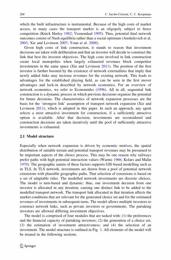
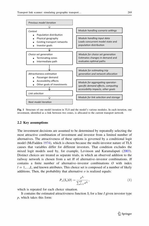
The model is comprised of four modules that are tasked with: (1) the preferences

and the financial capacity of partaking investors; (2) the generation of a choice set;

(3) the estimation of investment attractiveness; and (4) the selection of an

investment. The model structure is outlined in Fig. 1. All elements of the model will

be treated in the following sections.


123

2.2 Key assumptions

The investment decisions are assumed to be determined by repeatedly selecting the

most attractive combination of investment and investor from a limited number of

alternatives. The attractiveness of these options is governed by a conditional logit

model (McFadden 1974), which is chosen because the multi-investor nature of TLS

causes that variables differ for different investors. That condition excludes the

mixed logit models used by, for example, Levinson and Karamalaputi (2003).

Distinct choices are treated as separate trials, in which an observed addition to the

railway network is chosen from a set H of alternative–investor combinations. H

contains a finite number of alternative–investor combinations O with index

l = 1,…,L, and known attributes. This choice set is composed of a number of likely

additions. Then, the probability that alternative o is realized equals:

Po SojOð Þ ¼ eSoPO

l¼1 eSl; ð1Þ

which is repeated for each choice situation.

It contains the estimated attractiveness function Sl for a line I given investor type

p, which takes this form:

Choice set genera�onTermina�ng zonesIntermediate path

ContextPopula�on distribu�onPhysical geographyExis�ng transport networksInvestor goals

A�rac�veness es�ma�onPassenger demandAccessibility effectsOther goals of investments

Link selec�on

Previous model itera�on

Next model itera�on

Module handling scenario se�ngs

Module handling input dataLoads concurrent model state and popula�on distribu�on

Module for choice set genera�onEs�mates changes in demand andevaluates op�mal paths

Module for es�ma�ng trip genera�on and network alloca�on

Module for aggrega�ng operator-specific demand effects, compu�ng accessibility impacts, other goals

Module for link selec�on and storage

Fig. 1 Structure of one model iteration in TLS and the model’s various modules. In each iteration, oneinvestment, identified as a link between two zones, is allocated to the current transport network


123

Sl ¼ b0pROIl þ bnpXnl þ Rp þ Rl þ e; ð2Þ

where ROIl indicates the return on investment that investors presumably seek. This

is modelled by the estimated increase in passenger mileage on an investor’s net-

work, divided by the estimated costs of building the link; Xn is a vector of variables

used to capture other factors that affect the attractiveness of investment options; Rp

and Rl are alternative-specific and investor-specific random components that ensure

that the model does not yield multiple alternatives with identical probabilities; and eis a random disturbance.

The attractiveness of alternatives may differ per investor and may contain a

variety of different social or financial objectives. In the presented case study,

investor-specific attractiveness functions have been estimated using railway

investment choices taken while constructing the Dutch railway network and mainly

aim at increasing the revenues (reflected by passenger kilometres) on the investor’s

network; in other cases, these attractiveness functions need to be modified to reflect

case-specific investor goals or transport revenue types.

The selection of investment choices and the computation of investment

attractiveness is constrained by the following assumptions: (1) the territory is

divided into a given number of zones with estimable numbers of potential

passengers and/or movable goods, observed as origins (i) and destinations (j);

furthermore, (2) all zones are already connected by a preceding base communi-

cations network (base), so that spatial interactions already exist before the transport

mode is introduced. This network is expected to have maximum plausible

connectivity, so that the i to j travel distances Lbaseij obtained from this network

are the minimum realistic link lengths between two zones. A last constraining

assumption (3) is that the introduced transport mode is expected to lower

generalized travel costs per kilometre with a fixed relative cost improvement factor

u.We must emphasize that the value of u has a considerable impact on results of

the network allocation model. In this study, relative general cost improvements

depend on the transport speeds on the base network (Vbase) and the transport speeds

on the introduced network (V intr), so that V intr=Vbase ¼ u: One implication of the

model’s assumptions is that the links l in the modelled network have travel costs c

based on cbasel ¼ Ll=Vbase or cintrl ¼ Ll=V

intr; where Ll indicate link lengths. In the

case of public transport, it seems fair to adapt travel cost estimates with travel cost

penalties cp to simulate the effort involved in entering and exiting the introduced

transport network. This leads to fixed maximum obtainable travel cost improve-

ments between two zones, which can be computed as a ratio between minimum

new-mode travel costs cminij and existing travel costs cbaseij over the base network.

Maximum obtainable travel cost improvements are expressed as:

cbaseij =cminij ¼ Lbaseij =Vbase

� �= Lbaseij =V intr� �

þ 2cph i

; ð3Þ

in which maximum factor improvements are computed as base travel costs divided

by minimum achievable travel costs. Those factors in turn are computed as network


123

length divided by base transport mode speed, and minimum travel costs are com-

puted as the time used to transverse the same network length using the introduced

transport mode plus fixed travel cost penalties to enter and exit the introduced

transport mode. Thus, travel costs improvements are assumed to have a fixed

maximum, which has important ramifications for the selection of a choice set. This

can be seen in the following sections.

3 Choice set generation, investment selection and model accuracymeasures

Although in continuous space infinite potential links exist, computational limita-

tions force us to work with a limited choice set. This is justified by the property of

the conditional logit model demonstrated by McFadden (1974) that drawing a

limited number of alternatives leads to consistent estimates, provided that the true

choice process is described by the estimation procedure.1 TLS establishes a set of

discrete choice set alternatives by drawing samples with a reasonable probability of

selection using heuristic generation methods. In the attractiveness estimation

procedure, the built links are added to the choice set. Because of the dynamic nature

of TLS, the choice sets used in prediction are bound to differ from those used in the

estimation process, and we must therefore assume that the validity of estimated

attractiveness functions holds as long as investment options are selected with the

same criteria as the choice set used in the estimations.

We furthermore assume that link construction is incremental, which implies that

the most profitable link construction investments are selected first, and later, other

links are built as extensions to the investor’s network. To generate investment

options given these assumptions, a two-stage method is applied, which first deals

with the selection of terminating zones and later selects a plausible path between the

terminating points using corridor location searching methods. For a recent overview

of corridor location search methods, we refer to Scaparra et al. (2014). For this

section, it is necessary to explicitly discern links (l), which we consider as complete

investments between two terminating zones, and segments (s), which are the

separately observed lines in the model of which a link is composed.

3.1 Selecting terminating zones

The investment options are picked from a subset of zone pairs with high revenues

compared to costs. We compute a first estimate of the relative revenue-to-cost ratio

(RCR) of a potential new link by dividing additional passenger kilometres by

construction costs C:

1 An assumption of multinomial logit models is independence of irrelevant alternatives. There have been

some recent attempts to develop sampling strategies that may overcome this assumption; see, for

example, Guevara and Ben-Akiva (2013). However, it is beyond the scope of the present paper to try and

apply such methods, in particular since the generation of meaningful links is not trivial, as can be seen in

the rest of the paper.


123

RCRest1ij ¼ Lbaseij Test1

ij þ Test1ji � Tcurr

ij � Tcurrji

� �=Cest1

ij ; ð4Þ

where Lbaseij is a first estimate of link length defined as the shortest distance between i

and j in kilometres over the base network; T is the potential number of trips in both

directions with (est1) and without (curr) the new link; and Cest1ij is a first estimate of

construction costs.

Lengths and costs are assumed to be symmetric for both directions. We must

emphasize here that the link lengths and flows for potential investments are rough

estimates, because at this step in the selection procedure the optimal path of a

potential link between i and j is not yet known and as a consequence, neither are the

definitive travel times. The construction costs are obtained by finding the least-cost

path between zones given estimated construction costs for each potential network

segment. These construction costs are imposed on a fine-meshed network of

regularly distributed segments, which is elaborated upon later.

Potential trips T between zones are computed using a spatial interaction model

derived from Alonso’s General Theory of Movements (GTM) (Alonso 1978). It

must be emphasized that in the model these formulations can be easily substituted

by any other spatial interaction formulation, for example to take into account spatial

dependencies (Patuelli and Arbia 2013), heterogeneity or endogeneity (Donaghy

2010). For the selection of terminating zones, we compute trips T in three cases:

Tbaseij ¼ A

baseð1�cÞi

� ��1

PiPjf cbaseij

� �; and Abase

i ¼X

j

B1�hj Pjf cbaseij

� �; ð5aÞ

Tcurrij ¼ A

currð1�cÞi

� ��1

PiPjf ccurrij

� �; and Acurr

i ¼X

j

B1�hj Pjf ccurrij

� �; ð5bÞ

Test1ij ¼ A

est1ð1�cÞi

� ��1

PiPjf cest1ij

� �; and Aest1

i ¼X

j

B1�hj Pjf cest1ij

� �; ð5cÞ

where P represents zonal populations; cbaseij describes travel costs over the base

network; ccurrij describes current travel costs obtained from the network at the start of

the model’s iteration, thus including already allocated investments; cest1ij approxi-

mates travel costs if the potential investment is in place and is computed as

cest1ij ¼ Lbaseij =V intr; f(.) is a distance-decay function; c and h are parameters that

govern transport consumption elasticity for reduced travel costs; and Bj is a desti-

nation-specific constant that may be used to model congestion at destinations.

The computed levels of RCRest1ij are instrumental to select a pool of potentially

high revenue-to-cost ratio investments from which investment options in O are

selected. To exclude lines that offer relatively small total travel cost improvements

between two terminating zones, the line proposed in cest1ij must offer minimally half

the maximum travel cost improvements that may be obtained by substituting a base

network link with the link considered. Furthermore, intrazonal links and


123

symmetrical elements in the matrix are excluded. These criteria yield the following

selection dummy Zij:

Zij ¼ 1 if cest1ij =ccurrij

� �� 0:5 cest1ij =cbaseij

� �and i\j

0 otherwise

(

: ð6Þ

The criterion is admittedly chosen ad hoc, but seems to be a reasonable

assumption. This selection criterion is necessary to obtain a small choice set with

reasonably plausible alternatives. Note that in the case that cp[ 0; proposed links

between i and j also have an absolute minimum distance, because with lower

distances the rail link’s travel cost including waiting times does not offer sufficient

travel cost advantages. Finally, a fixed number of links between i and j with the

highest values of RCRest1ij Zij are selected as investment options.

3.2 Finding plausible paths

Simply connecting two zones without detours leads to the odd situation that the link

does not serve the zones that it passes. Optimal transport lines may ‘depart from the

straight line’ when a detour improves the balance between revenues and

construction costs (Morrill 1970). The links between selected terminating zone

pairs are therefore allowed to detour. Three factors are taken into account in the path

selection mechanism, namely potential revenues, construction costs and the overall

length of the link. These are used to obtain optimal paths given revenue-to-cost

ratios based on differently weighted combinations of the three factors. In all cases,

optimal paths are searched that meet a minimum travel cost improvement. Thus, the

maximum length of a link Lintrmaxij is a logical consequence of the maximum travel

cost improvements in (3), u; and the criterion used in Eq. (6), and is defined as:

Lintrmaxij ¼ V intr cbaseij � 2cp

� �=0:5 uð Þ

h i; ð7Þ

so that to achieve the maximum link distance, the maximum acceptable travel costs

are multiplied with the speed of the introduced transport model. To obtain optimal

paths, the continuous space in which built lines are determined is approximated by a

regularly formed network of potential line segments, in which equally distributed

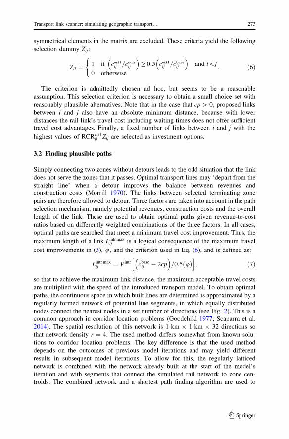
nodes connect the nearest nodes in a set number of directions (see Fig. 2). This is a

common approach in corridor location problems (Goodchild 1977; Scaparra et al.

2014). The spatial resolution of this network is 1 km 9 1 km 9 32 directions so

that network density r = 4. The used method differs somewhat from known solu-

tions to corridor location problems. The key difference is that the used method

depends on the outcomes of previous model iterations and may yield different

results in subsequent model iterations. To allow for this, the regularly latticed

network is combined with the network already built at the start of the model’s

iteration and with segments that connect the simulated rail network to zone cen-

troids. The combined network and a shortest path finding algorithm are used to


123

obtain a path with an optimal combination of revenues, construction costs and

length.

The revenue-cost indicators per segment s are computed as:

RCs ¼ Rs=Csð Þ1�k=Ls; ð8Þ

where Rs indicates estimated revenues obtained from the segment; Cs indicates costs

of segment construction; and Ls indicates segment lengths. This formula puts a high

weight on the revenue-to-cost ratio for low values of k, while the least lengthy path

is favoured in case k = 1. The method to estimate segment revenues will be

explained later. Construction costs are obtained from terrain characteristics. To

model additive network construction, already built railway segments are given a

very low cost of one. Note that more sophisticated cost structures for existing links

can be configured to simulate specific cooperation conditions. Finally, segment

lengths are primarily taken into account to ensure that the found path respects

Lintrij \Lintr maxij :

The inverse RC�1S is used as a measure of friction for each segment.

Subsequently, Dijkstra’s least-friction path algorithm is applied to find a path

between the terminating zones with the lowest total friction. Clearly, this approach

provides the possibility to obtain optimal paths according to a limited set of

parameterized factors. Because methods to obtain real parameter values for path

selection are not yet available, we iterate the importance of segment revenue-to-cost

ratios using the k parameter. Thus, the shortest path finding algorithm with RC�1S is

repeated in 40 iterations, in which k is gradually increased from zero to one. The

total inverse revenue-cost indicator of a path is:

Fig. 2 Schematic example of a regularly formed network with equally dispersed nodes shown as stars,segments from the centre node shown as regular lines and exemplary additional segments shown asdashed lines (left); example of the regularly formed network shown as dashed lines and potentiallyderived link shown as regular bold line positioned over a map of Amsterdam in 1842 (right)


123

RC�1TOT ¼

Xn

s¼1

RC�1S ¼

Xn

s¼1

Ls= Cs=Rsð Þ1�k: ð9Þ

For k = 0, this amounts to a distance-weighted sum of inverse revenue-to-cost

ratios, while for k = 1 it is simply total distance.

3.2.1 Estimating segment revenues

The revenues for each segment are estimated using a relatively straightforward

method. Explicitly taking into account revenues with different railroad line

geometries might require repetitive re-estimation of transport demand with various

path alternatives, which is computationally infeasible. We therefore take the

potential fare of a link as a proxy for potential revenues. This can be partially done

by taking into account the amount of people in the zones that a link connects. To

take into account that zones which are already connected to the network might

suffer from transport market saturation, we also include MS, which approximates

transportation market saturation at the origin and destination, so that:

MSi ¼Xn

j¼1

Lbaseij Test1ij � Lbaseij Tbase

ij

h i� Lbaseij Tcurr

ij � Lbaseij Tbaseij

h i� �

Lbaseij Test1ij � Lbaseij Tbase

ij

h i� � ; ð10Þ

in which the relative amount of passenger kilometres that can be obtained by

connecting a zone is estimated, given a base level of passenger kilometres

(Lbaseij Tbaseij ), the current level of passenger kilometres (Lbaseij Tcurr

ij Þ and the presumed

maximum number of passenger kilometres (Lbaseij Test1ij ). MSi is zero if the market is

fully saturated and one if there is no saturation whatever. Finally, the segments’

revenue levels are estimated as average non-saturated potential revenues in the

zones in which both the first and the last point of a segment are located:

Rs ¼1

2

Xn

i¼1

MSi Pis1 þ 1ð Þ þXn

i¼1

MSi Pis2 þ 1ð Þ" #

; ð11Þ

where revenues R of segments s are computed by means of the population P of zone

i in which the segment’s first point (s1) and last point (s2) are located and the zone’s

saturation factor MSi. One person is added to each zone to ensure that values of Rs

are above zero and thus warrant the computation of Eq. (9).

3.2.2 Optimal path selection

The iterative path finding method leaves 40 alternative paths with varying lengths.

These varying lengths signify a varying mix of revenue-cost optimization and length

reduction. We must acknowledge that in some cases the method captures many

alternatives with similar geometries, thus causing inefficiencies in the alternative

path generation. An extension of the model using recent advances in corridor


123

location problems such as those proposed by Scaparra et al. (2014) may be explored

in the future to solve this. To find the likely most profitable path, the passenger

kilometre increases obtained are recomputed for the whole i to j matrix, for which

the travel costs and travel distances between connected zones are repeatedly re-

estimated for every value of k. To do so, a dummy variable Qi indicates whether

zone i is connected to the alternative path at hand. Subsequently, the estimated

travel costs ccurrij and travel distances Lbaseij between all connected zones are updated

so that cest kij and Lest kij are defined for each alternative path k as:

cest kij ¼ path travel costs if QiQj ¼ 1

ccurrij otherwise

�

ð12Þ

Lestkij ¼ path travel distance if QiQj ¼ 1

Lbaseij otherwise

�

ð13Þ

which enables a more accurate estimate of revenues within the scope of the con-

nected zones. Lbaseij is used in (13) because a shortest length finding method on the

current network would always represent the geographically more efficient base

network, regardless of the state of the introduced transport mode. As with the first

estimate, revenues from not directly connected zones are neglected here. This is a

necessary evil to prevent excessive computational requirements in this stage of the

modelling exercise. Furthermore, the sum of segment construction costs is taken so

that the overall cost of the path for the iteration is known as Cest k. These new cost

and revenue estimates are used to estimate path revenue-cost indicators using:

Test kij ¼ A

est kð1�cÞi

� ��1

PiPjf cest kij

� �; and Aest k

i ¼Xn

j¼1

B1�hj Pjf cest kij

� �: ð14Þ

Finally, the overall length of the link is computed as Lintr k and used to obtain the

final revenue-cost ratios of all paths, so that:

RCRest k ¼Pn

i¼1

Pn

j¼1

Lest kij Test kij

� �h i=Cest k if Lintr k\Lintr max

ij

Lintr k� ��2

otherwise

8><

>:ð15Þ

In Eq. (15), the length of links is purposely squared to enforce that the shortest

path is only selected if no path is found that meets the Lintr maxij criterion.

Subsequently, the path with the highest value of RCR is selected. In this way, the

path with the highest estimated revenue-to-cost ratios is selected if a path that meets

the length criterion is found, and else the method picks the path with the shortest

overall length.

It is important to note that two additional restrictions are imposed on the path

decision method: first, we assume that railway network construction is incremental,

so that a) in all cases, if a link starts or terminates in a zone already connected by a

built line, the generated line must connect to the line already built there and b) the


123

links of an investor’s already existing network have negligible costs for the

considered expansion; second, to simulate that built railway links terminated outside

contemporary urban areas, the link may not start on a node less than 500 metres

away from the zone’s centroid. This approximates the distance between stations and

urban area centres that are observable in the historically built network.

3.3 Investment selection

Subsequently, the attractiveness of the investment options is computed. A wide

range of variables that deal with investor objectives can be computed here.

Increasing mileage, total transport flows or reduction in congestion due to

insufficient transport network capacity are, presumably, generally important reasons

for transport network investments. TLS therefore includes a module to model

expected transport flows on potential network extensions, on the investor’s

remaining network or on the whole transport network.

For all investment options generated in the choice set, the attractiveness is

estimated with the methods shown in the previous section, yielding values of Slspecific for each investor in a vector that is as long as the number of active investors

times the number of options. A very small random component is added to the

computed attractiveness values to warrant that two options do not have identical

attractiveness. Based on the estimated values, Eq. (1) is solved to obtain

probabilities for the considered investments. Ultimately, the investment with the

highest probability is selected. The new link and its relevant attributes are added to

the already existing network in a new file; this file may form the basis for the

evaluation of a subsequent investment if need be.

3.4 Measuring model accuracy

The primary goal of this paper is to demonstrate that modelling transport network

development with reasonable geographic accuracy is feasible. Xie and Levinson

(2011) use rank correlations to verify to what degree their model captures the

sequence of links accurately. Unfortunately this only works if the modelling is

restricted to the topology of the observed network, which is not the case in TLS. A

visual inspection of allocation results yields useful insights, but does not provide the

possibility to assess the accuracy of the model at hand in a balanced and objective

manner, for which accuracy indicators and a baseline comparison are necessary.

Although many network-based indicators to compare modelling results are

conceivable such as the ones provided by Rodrigue et al. (2006), we concentrate

on two indicators that deal with geographically relevant aspects of the results. One

indicator measures to what degree the same zones are connected as have been

connected by the historically built line; and the other indicator measures differences

in travel times. Because we assume that model accuracy is more critical for

populous areas, all indicators are weighted by population. Weighted connection

error WCE is thus measured as:


123

WCE ¼ 1�Xn

i¼1

Pobservedi Xmodelled

i Xobservedi

� �=Xn

i¼1

Pobservedi Xobserved

i

!

; ð16Þ

where X is a zone-specific dummy that takes the value one when a municipality is

connected by the modelled and observed railway networks, and zero otherwise.

Essentially this measure indicates to which degree the zones that were connected

by the really built network are being connected by the modelled network, and it thus

only measures double positives. We believe this is sufficient for the scope of this

paper but plan to develop a wider range of indicators in further exercises. The

weighted mean average absolute percentage travel-time error (‘WMAPE’) is

measured as:

WMAPE ¼ 1

n

Xn

i¼1

Xn

j¼1

Pobservedi Abs cobservedij � cmodelled

ij

h i

Pobservedi cobservedij

0

@

1

A; ð17Þ

where the absolute population-weighted differences between the observed and

modelled travel times are expressed as percentage of the observed travel times, and

the final results are subsequently averaged. Naturally, in both the modelled and

historical networks the same rules regarding waiting times and travel speeds are

upheld to enable a fair comparison of travel times.

To ensure a meaningful comparison, modelled networks are compared with the

state of the historically built network that is closest to the modelled network in terms

of length. Thus, if in the fourth investment turn, a modelled network has a length of

1000 km, subsequent individual historical investments are tested for cumulative

length until the historical investment is selected that brought the historically built

network the closest to a 1000-km cumulative length. The network comprising that

and previous investments is selected for comparison. In addition, the population

levels of the year in which the selected historical investment is built are selected to

serve as weights for the presented indicators.

4 Case study

In this section, we present an effort to simulate the development of the Dutch

railway network in the nineteenth and early twentieth century using TLS.

Investment attractiveness functions were fitted on observed transport network

investments. First the history of the development of that railway network is

summarized, after which the model set-up, main assumptions and estimation of

transport link attractiveness are outlined.

4.1 The development of the Dutch railway network

The first railway in the Netherlands opened in 1839 (Veenendaal 2008). It was

operated by the ‘Holland Iron Railway Company’ (HSM) and linked Amsterdam to

Haarlem. It was soon extended towards Rotterdam. Subsequently, competing


123

companies built their own lines in the Netherlands. More than ten operators have

separately provided railway services on railway links in the Netherlands. The Dutch

government began participating actively by building state lines defined in the

Railway Acts of 1860 and 1875. Most of those state lines were run by the ‘State

Railways’ (SR), a private company which leased lines owned by the state. In 1878, a

third Act followed that allowed for the cheaper construction of railways, if operated

with slow light trains. Supported by attractive loans from the Dutch State and

subsidies from local governments (Doedens and Mulder 1989), this Railway Act

incited the construction of ‘local tracks’ that typically connected rural areas to the

main railway network (Veenendaal 2008) and were often subsidized by local

governments. In this paper, we treat state involvement as the introduction of other

types of investors with distinct preferences in the railway development playing field.

After an initial slow start, railway development began to pick up speed in the

1850s when additional operators and the Dutch state began to participate in network

development (see Fig. 3). In total, 25 operators have operated rail lines in the

country according to the data observed in this study. Increasing competition led to

considerable growth in the length of the railway network between 1860 and 1890.

Many operators could not keep up, and in 1890 the infrastructure of the third largest

railway operator (‘NRS’) was nationalized. After this, the railway transport market

was almost completely in hands of HSM and SR. In 1917, decreasing revenues

forced HSM and SR to cooperate within an institutional framework in which Dutch

policies regarding railroad operations shifted from pro-competition to pro-cartel.

Finally, in 1936 all railway infrastructure was nationalized, and operations were

continued by the state. By 1936, opportunities for further railway network

expansion evidently were exhausted and the network did not expand any further

until the 1980s.

4.2 Population distribution, network speeds and network ownership

Based on Veenendaal (2008) and Stationsweb (2009), the historical railway network

development in the Netherlands has been reconstructed in a GIS database that also

contains population counts from 1830 to 1930 in 1076 municipalities. The data,

furthermore, build on the same assumptions as in Koopmans et al. (2012), of which

we now list the most important ones. The study area is assumed to already have an

underlying network of paths that connects all municipalities with each other. In the

0

1

2

3

1830 1860 1890 1920Leng

th (i

n 1,

000

km)

Year

All railways

State-built lines

Fig. 3 Length of railway lines in the Netherlands over time


123

nineteenth century, horse-drawn boats through the country’s tow canals were the

main long distance travel mode and often the only alternative to walking to most

people. They operated at a speed that was but slightly faster than walking. We must

acknowledge that the historical networks of paved roads and tow canals are not

taken into account explicitly; instead, just as Koopmans et al. (2012), we consider

both networks to be regional substitutes for each other that are approximated using

one simplified network. In the case study, that network connects each municipality

with its five nearest neighbours. A speed Vbase ¼ 6 km=h is maintained as the

average speed to traverse this network to proxy movement over roads and

waterways. We assume this is a reasonably accurate assumption for the Netherlands.

One model variant is run with Vbase ¼ 4 km=h to test model sensitivity for this

setting.

Municipalities are represented by means of their geographic centres. The base

network has direct connections between those centroids. The rail network is

connected to those centroids through connector road links. Train schedules or the

accelerating and decelerating of trains are not explicitly modelled, but are

approximated by imposing relatively low average speeds for the introduced

transport links. To proxy that passengers lose some time with entering and exiting

the rail network as well as with transferring between physically separate rail

networks, a relatively small travel cost penalty cp ¼ 10 min is given to all

connectors between rail networks and municipalities.

When assessing the attractiveness of investments, links of the previously

modelled network extensions are included as well as the underlying network. As

given in Sect. 4.3, passenger transport demand is an important reason for

investment. The level of demand depends on generalized transport cost, which is

proxied by travel time, and on price elasticity. This makes the modelled speeds on

the railway network and assumptions on price elasticity a key factor for network

outcomes. To take these factors into account, we present scenarios with varying

travel-time improvements and with varying assumptions on price elasticity of

passenger transport demand. Construction costs, passenger demand and price

elasticity have been estimated using observed data. Details of the method used, data

and results can be found in Appendices 1 and 2.

To model railway network expansion in a case with multiple investors with

varying objectives, five independent investors are simulated. This set of investors

consists of two regular private investors, two private local line investors and the

state and roughly resembles the playing field during Dutch railway construction.

The regular private investors partake in investments from the model start. The state

partakes from 1860; local line investors from 1879. At any point, the investment–

investor combination with the highest probability is selected. All investors are

eligible to the same investments with attributes that may differ per investor; ten

investment options are available in every round. The built lines are assumed to be

operated by the building investor, so that all revenues from an investor’s line are

therefore assumed to fall to that investor. In the presented case study, the modelled

investment sequence starts in 1839, with one investment allowed every year. After

an investment, an operator is excluded one round to simulate financial recuperation


123

and evaluation of the investment. Municipal population counts are updated every

decade. If the model does not find any suitable investments, it skips years to a

following decade; if it does no longer find suitable investments in 1930, the network

expansion sequence ends.

Because both travel speed improvements and price elasticity can only be roughly

estimated, we present a range of scenarios in which those assumptions vary

considerably. In one scenario, train speeds are three times faster than the pedestrian

network, so that average speed of train trips is defined as V intr ¼ 18 km=h and

Vbase ¼ 6 km=h, and total municipal transport consumption is affected by changes

in travel times (scenario A). The level of elasticity is given as c as in Eq. (5a). In

scenario C, trains speeds are 7.5 times faster than the pedestrian network, with

V intr ¼ 30 km=h and Vbase ¼ 4 km=h, while municipal transport consumption is

inelastic (scenario C). In four other scenarios, train speeds are five times faster, with

V intr ¼ 30 km=h and Vbase ¼ 6 km=h, while municipal transport consumption is

again inelastic (scenarios B1 to B4). In scenario B1, only train speed and transport

consumption are changed. To understand the sensitivity of the model for other

model assumptions, further variations in rules are simulated in scenarios B2 to B4.

In scenario B2, investors are not excluded in the round directly following an

investment. In scenarios B3 and B4, only regular private investors are modelled, so

that state lines and local line investors are excluded in the simulations. In scenario

B3, investors are assumed to be competitors, while in scenario B4, investors are

assumed to be co-dependent. Co-dependency is approximated by adding the relative

change in passenger mileage on the competitor network to the attractiveness

function of an investment. All used scenarios are summarized in Table 1. We must

acknowledge that this is not a complete sensitivity analysis in which all assumptions

are varied independently. That is an almost impossible task, given the number of

assumptions in the model and the minimum 10 days needed for one model run even

Table 1 The scenarios used

Scenario Description u and

ðV intr=VbaseÞc

A Slow trains, elastic consumption 3 (18/6) 0.3

B1 Fast trains, inelastic consumption 5 (30/6) 0

B2 As B1, but investors are not excluded directly after an investment 5 (30/6) 0

B3 As B1, but only private investors 5 (30/6) 0

B4 As B3, but change in passenger mileage on competitor network is a

factor for investment attractiveness

5 (30/6) 0

C Slower walking speeds, B5 parameters 7.5 (30/4) 0

Rietveld and

Bruinsma

Reproduction of Rietveld and Bruinsma (1998) 5 (30/6) 0

Parameter u indicates relative speed improvement as a ratio of the speed of the introduced transport mode

V intr versus the speed of prior transport modes Vbase; see Sect. 2.2. Parameter c indicates transport

consumption elasticity, see Eqs. (5a)–(5c)


123

on a, at the time of writing, high-end 2.6 Ghz Xeon PC. In any case, such a

sensitivity analysis is outside of the scope of this paper. For future applications, we

propose to pinpoint parameters that are crucial to conclusion validity and test model

sensitivity for these parameters.

Measuring performance is meaningless without a baseline comparison of

accuracy. To compare relative model performance, the model described by Rietveld

and Bruinsma (1998) has been approximated using the TLS framework. The

Rietveld and Bruinsma method repeatedly adds a straight line between the two cities

that yield the highest expected return on investment. Only the 35 most populous

cities in the country are taken into account. Costs are equal to length, with the

exception of links that cross large waterbodies; those links cost a factor 20 more. No

fixed costs or minimum travel times are applied, and varying investor differences

are not accounted for. This model is implemented in TLS by selecting the highest

value of Eq. (4), taking into account only the original subset of 35 cities. One link is

added in every model iteration. All links are assumed to be private lines. The

plausible paths method in Sect. 3.2 is adapted to exclude variation in estimated link

revenues. The allocation procedure is finished when the pool of available cities is

exhausted. We must note that a comparison with a socially optimal network (Li

et al. 2010) is also useful here; further work is needed to establish norms for

optimality and generate a meaningful optimum.

4.3 Investment choices

Because inland water transport provided the Dutch freight sector, a cheap substitute

for rail passenger transport was a particularly important service for Dutch railway

investors (Filarski and Mom 2008). Furthermore, railways have been considered to

possess unifying qualities (Veenendaal 2008), which were presumably sought after

by the Dutch administration in the nineteenth century. Although the ‘United

Provinces’ created in the seventeenth century had become a centrally led monarchy

by 1806, the country was only starting to form a political union when the railways

began to develop (Kossmann 1986).

To investigate the motives of investment decisions in the development of the

Dutch railway network, the conditional logit choice model in (1) has been fitted on

sets of built and unbuilt railway links. Investments were separated into regular

private lines, private lines that comply with local track legislation, and state lines.

As noted before, return on investment is assumed to be the key driving force.

Revenues are expected to be linear with travelled distances; this cannot be validated

because data on historical ticket pricing structures are currently unavailable. We

thus implicitly assume that pricing levels were equal throughout the country

regardless of regulation or level of competition. This is presumably not true, and the

consequences are worth exploring in follow-up research.

Next to return on investment a number of other variables are taken into account

in the attractiveness function. Amongst those, changes in the level of inequality of

accessibility values proxy the endeavour of in particular government investors to

reduce national disparities in economic opportunity. It is computed as changes in the

Theil index of municipal accessibility levels. This variable takes this form:


123

IAl ¼ 1001

n

X

i¼1

Aopt li

Aopt l� lnA

opt li

Aopt l

!

� 1

n

X

i¼1

Acurri

Acurr� lnA

curri

Acurr

� �" #

; ð18Þ

Acurri ¼

X

i6¼j

Pjf ccurrij

� �; A

opt li ¼

X

i 6¼j

Pjf copt lij

� �; ð19Þ

so that differences in the distributions of current accessibility levels Acurri and

accessibility levels Aopt li , which include the investment option l, are taken into

account. Thus, Acurri is a measure of accessibility with initial travel times; A

opt li

describes accessibility levels when including the travel costs improvements from the

potential investment.

Furthermore, two dichotomous variables indicate whether a link connects to

other links in the entire railway network and in particular to links on the operator’s

network. Connecting to the existing rail network is presumed to add option values

for revenues of later connections to further cities; operational cost reductions for an

operator because inventory can be kept at one centralized point; and furthermore,

operators might consider that having an extensive connected network brings

prestige. Another dichotomous variable indicates whether a link provides a first

connection to provincial capitals or to the country capital city, Amsterdam.

Connecting to these cities might be attractive if investors expected larger growth of

the passenger market in those cities and might have prestige value as well. Yet

another dichotomous variable indicates whether a link connects municipalities on

the country border. This variable represents attempts to profit from international

passenger and mail transport. A last dichotomous variable indicates whether a link

connects to a sea harbour. This variable represents endeavours to connect Dutch sea

harbours with their hinterlands by means of rail for the sake of goods transport.

The built links in the choice set were derived from the database of constructed

railway links. We have used the following definition of a link: a link connects at

least two existing nodes (railway junctions, stations or municipalities) and has been

realized by an investor as one integrated project within a limited number of years.

We assume that the results of the applied models are more accurate in the case of

longer links, and therefore weight the results of Eq. (1) by the length of built link o,

normalized by the average length of all built links in period t so that the total

number of observations in the choice model is not affected. To generate a choice set

of unbuilt links, we applied the following procedure: (1) a set of 50 alternatives was

generated for all links that were built in one decade; (2) to simulate that investors

presumably had limited capital in particular in the early stages of network

development, the costs of railway construction of an alternative could not exceed

the costs of a built railway in a longer period (either 1839–1859, 1859–1889 or

1889–1929); (3) selection of terminating municipalities and the routing of the

intermediate path were not affected by the transport market saturation of

municipalities MS.

Going through the results in Table 2, one finds that private line investors were

focused on high return on investments, while, compared with other alternatives with

reasonably good return on investments, local line and state investments were rather


123

indifferent to maximizing their returns on investment. We must note that the results

of an alternative model specification that included passenger mileage change on the

whole network in the return on investment yielded worse results for all operators

Table 2 Results of fitting a conditional logit model on the attributes of the built and automatically

generated unbuilt lines in the Dutch railway network

Scenario A B1

Coefficient Z score Coefficient Z score

Return on investment

Private lines 0.64** (3.84) 1.28** (3.81)

Private local lines 0.11 (0.58) 0.38 (0.79)

State lines 0.46 (1.64) 0.40 (0.81)

Change in accessibility inequality

Private lines 6.59** (3.03) 8.16** (3.10)

Private local lines -21.00** (-3.83) -20.53** (-3.70)

State lines -20.89** (-4.48) -23.20** (-5.10)

Connects operator network

Private lines 1.69 (1.76) 1.69 (1.78)

Private local lines 2.42** (3.11) 2.22** (2.87)

State lines 3.83* (2.57) 4.07** (2.76)

Connects railway network

Private lines -0.65 (-1.05) -0.71 (-1.17)

Private local lines 0.05 (0.12) 0.14 (0.31)

State lines -2.68** (-3.41) -2.77** (-3.36)

First connection to a provincial capital

Private lines 3.86** (4.62) 3.77** (4.55)

Private local lines N/A N/A

State lines -1.67 (-1.34) -1.90 (-1.47)

Connects border zone

Private lines 3.45** (4.96) 3.71** (5.26)

Private local lines -0.59 (-0.52) -0.52 (-0.45)

State lines 0.06 (0.06) -0.10 (-0.10)

Connects sea harbour

Private lines -0.35 (-0.53) -0.43 (-0.64)

Private local lines -0.11 (-0.17) -0.01 (-0.01)

State lines 1.46* (2.15) 1.41* (2.11)

McFadden’s Pseudo-R2 0.57 0.57

AIC 262.95 265.37

Coefficients marked by * are significant at the 0.05 level; those marked by ** are significant at the 0.01

level. All others are not. In the provincial capital variable, coefficients for local lines are missing because

of insufficient variance in the data. The coefficients are set to zero in the later modelling exercise. In

Scenario A, N = 3160; in Scenario B1, N = 3193


123

(results available upon request). We thus conclude that, consistent with other

findings (Xie and Levinson 2011), the various operators were primarily preoccupied

with the results for their own network. While private lines increased the disparities

in accessibility in the country, private local lines and state lines aimed to decrease

those disparities. The state presumably had political aims to decrease disparities in

accessibility. These aims were, clearly, further enforced through subsidies and loans

that accompanied the local railway act. All parties aimed to connect their new

investments to their own network. The poor significance values in case of regular

private lines presumably are due to the relatively large number of operators starting

new networks in the early stages of network development. Private investors were

apparently indifferent to whether their networks connected to competitors, while,

surprisingly, state investments actively avoided connecting to other networks.

Establishing the first connection to provincial capitals was sought after by private

investors. Connecting border zones (and, implicitly, foreign railway networks) was

also sought after by private line investors. In contrast, connecting sea harbours was

sought after only by the Dutch state, possibly to provide a stimulus to the Dutch

ports or for defensive purposes. The lack of interest from private parties seems to

confirm that in the Netherlands, there was a very limited market for the overland

transport of goods (Filarski and Mom 2008).

5 Simulation results

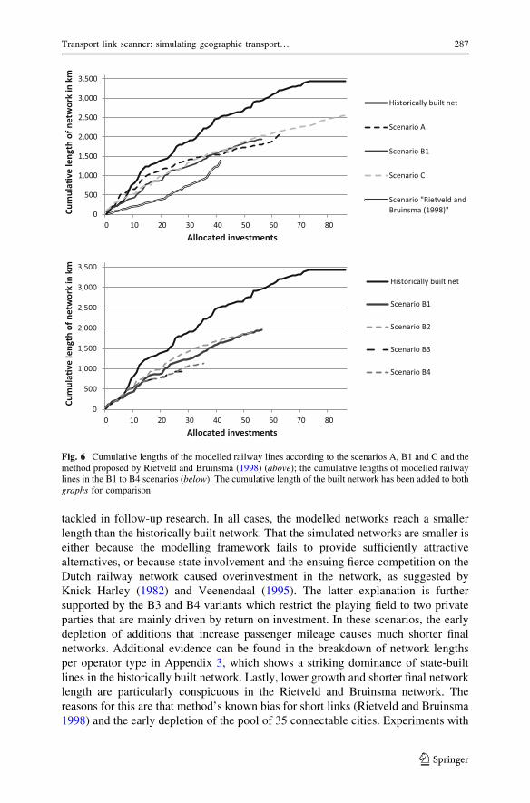
The historically built network and the allocation results for various scenarios are

plotted in Figs. 4 and 5. The modelling efforts have yielded networks that are

particularly dense in the Western, most urbanized part of the country. In contrast,

the northern, eastern and southern parts of the country are much less served. In

particular, the southwest of the country seems to gain more investments than built in

reality, while especially lines in the eastern and south-eastern parts of the country

are underrepresented in the modelling results. An in-depth investigation of this bias

is planned in follow-up research.

The differences in network shapes and network ownership are striking. In all

cases, private lines mostly function as trunk lines, with the state providing

peripheral extensions to the trunk network and local lines providing connections

between trunk lines. With the exception of scenario C, local lines do not seem to

have a dominant feeder function. The density of the trunk line network depends on

overarching conditions: for example, with a lower value of / the trunk network

appears to be more extensive (cf. scenario A vs scenario B1). Interestingly, in the

B2 variant, one operator obtains complete monopoly in the private lines and

expands that network much more than happens in a more competitive setting (cf.

scenario B1). Possibly the existence of greater network externalities allows for a

greater density in the final network of the monopolist.

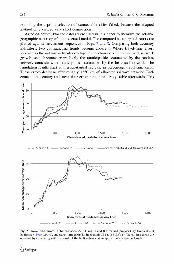
The total cumulative length of the historical and modelled networks is shown in

Fig. 6. It is clear that after the first five investments or so, the model allocates

network investments in smaller chunks than the historically built network, causing

the lower per investment growth of the modelled networks. This bias deserves to be


123

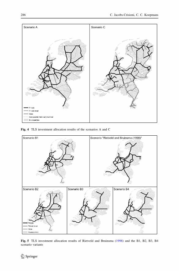
Fig. 4 TLS investment allocation results of the scenarios A and C

Fig. 5 TLS investment allocation results of Rietveld and Bruinsma (1998) and the B1, B2, B3, B4scenario variants


123

tackled in follow-up research. In all cases, the modelled networks reach a smaller

length than the historically built network. That the simulated networks are smaller is

either because the modelling framework fails to provide sufficiently attractive

alternatives, or because state involvement and the ensuing fierce competition on the

Dutch railway network caused overinvestment in the network, as suggested by

Knick Harley (1982) and Veenendaal (1995). The latter explanation is further

supported by the B3 and B4 variants which restrict the playing field to two private

parties that are mainly driven by return on investment. In these scenarios, the early

depletion of additions that increase passenger mileage causes much shorter final

networks. Additional evidence can be found in the breakdown of network lengths

per operator type in Appendix 3, which shows a striking dominance of state-built

lines in the historically built network. Lastly, lower growth and shorter final network

length are particularly conspicuous in the Rietveld and Bruinsma network. The

reasons for this are that method’s known bias for short links (Rietveld and Bruinsma

1998) and the early depletion of the pool of 35 connectable cities. Experiments with

0

500

1,000

1,500

2,000

2,500

3,000

3,500

0 10 20 30 40 50 60 70 80

Cum

ula�

ve le

ngth

of n

etw

ork

in k

m

Allocated investments

Historically built net

Scenario A

Scenario B1

Scenario C

Scenario "Rietveld andBruinsma (1998)"

0

500

1,000

1,500

2,000

2,500

3,000

3,500

0 10 20 30 40 50 60 70 80

Cum

ula�

ve le

ngth

of n

etw

ork

in k

m


Historically built net

Scenario B1

Scenario B2

Scenario B3

Scenario B4

Fig. 6 Cumulative lengths of the modelled railway lines according to the scenarios A, B1 and C and themethod proposed by Rietveld and Bruinsma (1998) (above); the cumulative lengths of modelled railwaylines in the B1 to B4 scenarios (below). The cumulative length of the built network has been added to bothgraphs for comparison


123

removing the a priori selection of connectable cities failed, because the adapted

method only yielded very short connections.

As noted before, two indicators were used in this paper to measure the relative

geographic accuracy of the presented model. The computed accuracy indicators are

plotted against investment sequences in Figs. 7 and 8. Comparing both accuracy

indicators, two contradicting trends become apparent. Where travel-time errors

increase as the railway network develops, connection errors decrease with network

growth, as it becomes more likely the municipalities connected by the random

network coincide with municipalities connected by the historical network. The

simulation results start with a substantial increase in percentage travel-time error.

These errors decrease after roughly 1250 km of allocated railway network. Both

connection accuracy and travel-time errors remain relatively stable afterwards. This

0

10

20

30

0 500 1,000 1,500 2,000 2,500

emit levart

nirorreegatne crep

naeM

Kilometres of modelled railway lines

Scenario A Scenario B1 Scenario C Scenario "Rietveld and Bruinsma (1998)"

0

10

20

30

0 500 1,000 1,500 2,000 2,500

emi tlev art

niro rreegatnecre p

na eM


Scenario B1 Scenario B2 Scenario B3 Scenario B4

Fig. 7 Travel-time errors in the scenarios A, B1 and C and the method proposed by Rietveld andBruinsma (1998) (above), and travel-time errors in the scenarios B1 to B4 (below). Travel-time errors areobtained by comparing with the result of the built network at an approximately similar length


123

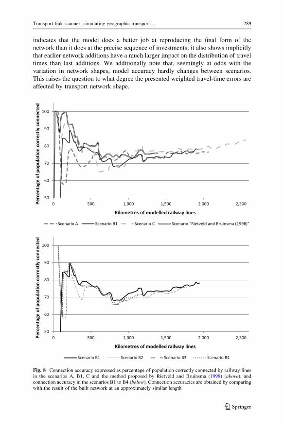
indicates that the model does a better job at reproducing the final form of the

network than it does at the precise sequence of investments; it also shows implicitly

that earlier network additions have a much larger impact on the distribution of travel

times than last additions. We additionally note that, seemingly at odds with the

variation in network shapes, model accuracy hardly changes between scenarios.

This raises the question to what degree the presented weighted travel-time errors are

affected by transport network shape.

50

60

70

80

90

100

0 500 1,000 1,500 2,000 2,500

det cenn ocyltce rroc

noita lupo pf oega tnec reP



50

60

70

80

90

100

0 500 1,000 1,500 2,000 2,500

detce nn ocyltcer roc

noit alu popf oegat necr eP


Scenario B1 Scenario B2 Scenario B3 Scenario B4

Fig. 8 Connection accuracy expressed as percentage of population correctly connected by railway linesin the scenarios A, B1, C and the method proposed by Rietveld and Bruinsma (1998) (above), andconnection accuracy in the scenarios B1 to B4 (below). Connection accuracies are obtained by comparingwith the result of the built network at an approximately similar length


123

6 Closing remarks

This paper presents transport link scanner, a model that simulates the expansion of

transport networks. Based on a conditional logit method, the model repeatedly

selects one most attractive link from a choice set to add to the expanding network.

That choice set is generated using heuristics with the goal to obtain a limited set of

relevant, geographically plausible links. The model outlined in this paper explicitly

allows the empirical estimation of preferences in a context with multiple actors with

possibly different characteristics. It allows to test, amongst others, the impact of

investor preferences, transport revenue structures and network effects on the final

outcomes of a transport network.

A practical application of the model is presented as well. This exercise focuses

on the expansion of the Dutch railway network in the nineteenth and early

twentieth century and compares the model’s accuracy with a previous attempt by

Rietveld and Bruinsma (1998). The results presented show that the early expansion

of the Dutch railway network is simulated by TLS with similar accuracy as by

Rietveld and Bruinsma, without the necessity of an a priori selection of

connectable cities. The results corroborate findings that transport network

expansion follows a clear rationale (Rietveld and Bruinsma 1998; Xie and

Levinson 2011; Levinson et al. 2012), show that the modelling rationale can

simulate network expansion processes with some success and illustrate that

institutional and economic settings may have a profound effect on network

expansion outcomes. Future research may be necessary to further improve the

accuracy of the model and measure its performance in terms of characteristic

spatial network metrics (Rodrigue et al. 2006). One other useful addition would be

the inclusion of socially optimal networks (Li et al. 2010) that would enable

exploration of how competitive investment decisions can be directed towards social

optima (Anshelevich et al. 2003). Nevertheless, we conclude that the model

appears to become a useful tool for academic studies and policy evaluations.

Acknowledgements This work has profited immeasurably from the many inputs given by Piet Rietveld,

whose untimely death has prevented him from seeing these final results. We must also thank Aart Huijg,

Peter Groote, Maarten Hilferink, Martin van der Beek, the Dutch Railway museum and three anonymous

reviewers, who have all had an important role in the preparation of this paper.

Open Access This article is distributed under the terms of the Creative Commons Attribution 4.0

International License (http://creativecommons.org/licenses/by/4.0/), which permits unrestricted use, dis-

tribution, and reproduction in any medium, provided you give appropriate credit to the original

author(s) and the source, provide a link to the Creative Commons license, and indicate if changes were

made.


123

http://creativecommons.org/licenses/by/4.0/

Appendix 1: Transport link construction costs

In the choice set generation and in the estimation of investment attractiveness, the

construction costs of distinct investments come into play. In this study, the costs that

are taken into account are a fixed cost and costs linked with the geography that the

proposed link overcomes. For the sake of simplicity, the costs for maintenance,

personnel and inventory are currently ignored in the model. In the case study, the

costs of constructing a link have been estimated using an ordinary least squares

(OLS) regression of the following equation:

Cl ¼ b0RIVERl þ b1HARDSOILSl þ b2SOFTSOILSl þ e ð20Þ

in which guilders of recorded costs of nineteenth-century rail construction

projects in the Netherlands are explained by a constant and traversed metres of

river, hard and soft soils. The hard soils class contains gravel, sand and loam.

The soft soils class contains clay and peat. The recorded costs describe the costs

imbued by the Dutch state in a number of network expansions between 1860 and

1880. These costs have been inflated to the 1913 level and are assumed to be

fixed (in real terms) over time. For the comparison of investment options, the

geographic distribution of cost factors is much more important than temporal

variations. Therefore, we expect that this assumption does not substantially

affect the results of this article. The OLS estimation results are given in Table 3.

Unfortunately, the exact locations of built-up land in the Netherlands in the

nineteenth century and the costs of building railways through such built-up areas

are not precisely known, so that we cannot model the presumably high costs of

constructing railways in already urbanized areas. We note, however, that the

Netherlands were a mainly rural country in the nineteenth century. Moreover,

railway stations and railway lines were mainly built at the edges of the then

existing cities.

Table 3 Estimated factors

contributing to the costs of

constructing a railway line

* Estimates significant at the

0.05 level. N = 38. R2 = 0.14

Coefficient t statistics

Constant 1,980,280.00* 2.39

Meter of river 2760.61 1.76

Meter of hard soil 12.38 0.55

Meter of soft soil 64.57* 2.57


123

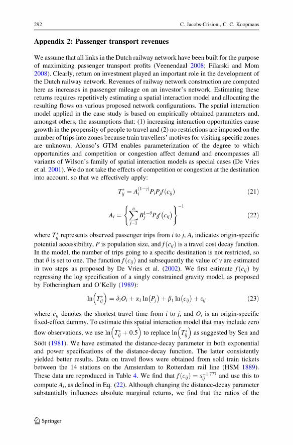
Appendix 2: Passenger transport revenues

We assume that all links in the Dutch railway network have been built for the purpose

of maximizing passenger transport profits (Veenendaal 2008; Filarski and Mom

2008). Clearly, return on investment played an important role in the development of

the Dutch railway network. Revenues of railway network construction are computed

here as increases in passenger mileage on an investor’s network. Estimating these

returns requires repetitively estimating a spatial interaction model and allocating the

resulting flows on various proposed network configurations. The spatial interaction

model applied in the case study is based on empirically obtained parameters and,

amongst others, the assumptions that: (1) increasing interaction opportunities cause

growth in the propensity of people to travel and (2) no restrictions are imposed on the

number of trips into zones because train travellers’ motives for visiting specific zones

are unknown. Alonso’s GTM enables parameterization of the degree to which

opportunities and competition or congestion affect demand and encompasses all

variants of Wilson’s family of spatial interaction models as special cases (De Vries

et al. 2001). We do not take the effects of competition or congestion at the destination

into account, so that we effectively apply:

T�ij ¼ A

1�cð Þi PiPjf ðcijÞ ð21Þ

Ai ¼Xn

j¼1

B1�hj Pjf cij

� �( )�1

ð22Þ

where T�ij represents observed passenger trips from i to j, Ai indicates origin-specific

potential accessibility, P is population size, and f ðcijÞ is a travel cost decay function.In the model, the number of trips going to a specific destination is not restricted, so

that h is set to one. The function f ðcijÞ and subsequently the value of c are estimated

in two steps as proposed by De Vries et al. (2002). We first estimate f ðcijÞ by

regressing the log specification of a singly constrained gravity model, as proposed

by Fotheringham and O’Kelly (1989):

ln T�ij

� �¼ diOi þ a1 ln Pj

� �þ b1 ln cij

� �þ eij ð23Þ

where cij denotes the shortest travel time from i to j, and Oi is an origin-specific

fixed-effect dummy. To estimate this spatial interaction model that may include zero

flow observations, we use ln T�ij þ 0:5

� �to replace ln T�

ij

� �as suggested by Sen and

Soot (1981). We have estimated the distance-decay parameter in both exponential

and power specifications of the distance-decay function. The latter consistently

yielded better results. Data on travel flows were obtained from sold train tickets

between the 14 stations on the Amsterdam to Rotterdam rail line (HSM 1889).

These data are reproduced in Table 4. We find that f ðcijÞ ¼ s�1:777ij and use this to

compute Ai, as defined in Eq. (22). Although changing the distance-decay parameter

substantially influences absolute marginal returns, we find that the ratios of the


123

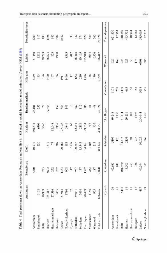
Table

4Totalpassenger

flowsonAmsterdam

–Rotterdam

railway

linein

1888usedin

spatialinteractionmodel

estimation.Source:

HSM

(1889)

Amsterdam

Bennebroek

Delft

Haarlem

Haarlem

merliede

Hillegom

Leiden

Noordwijkerhout

Amsterdam

6210

10,977

380,371

26,101

3349

51,450

3709

Bennebroek

6108

220

6304

252

143

1262

917

Delft

10,939

225

3346

72

186

20,223

183

Haarlem

385,317

5802

3317

19,454

2420

26,873

4026

Haarlem

merliede

27,516

252

77

18,948

167

823

145

Hillegom

3455

232

207

2459

159

36

1900

1504

Leiden

51,914

1333

20,167

27,028

854

1911

8652

Noordwijkerhout

3780

908

184

3849

143

1496

8393

Rijsw

ijk

52

42

5737

63

10

17

412

33

Rotterdam

39,641

967

100,856

12,751

682

652

46,418

332

Schiedam

5434

137

35,343

2189

112

210

10,105

374

TheHague

90,409

1322

134,445

29,354

386

1326

205,918

1629

Voorschoten

1156

253

1405

653

51

146

6064

559

Warmond

955

187

214

935

48

170

6576

765

Totalarrivals

626,676

17,870

313,149

488,250

48,324

12,229

386,417

22,828

Rijsw

ijk

Rotterdam

Schiedam

TheHague

Voorschoten

Warmond

Totaldepartures

Amsterdam

56

42,685

5197

89,248

1171

926

621,450

Bennebroek

41

841

120

1330

257

168

17,963

Delft

5495

101,960

34,475

131,814

1439

223

310,580

Haarlem

64

13,505

2153

29,231

665

925

493,752

Haarlem

merliede

11

483

91

381

50

50

48,994

Hillegom

17

736

238

1396

153

176

12,668

Leiden

417

46,394

10,025

204,044

6018

6308

385,065

Noordwijkerhout

29

315

368

1626

555

686

22,332


123

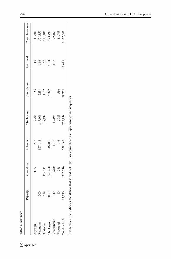
Table

4continued

Rijsw

ijk

Rotterdam

Schiedam

TheHague

Voorschoten

Warmond

Totaldepartures

Rijsw

ijk

1173

707

3266

156

16

11,684

Rotterdam

1200

127,148

245,406

2231

366

578,650

Schiedam

719

129,133

46,439

1147

162

231,504

TheHague

3853

245,450

46,415

15,372

3120

778,999

Voorschoten

149

2220

1106

15,194

507

29,463

Warmond

19

335

146

3083

510

13,943

Totalarrivals

12,070

585,230

228,189

772,458

29,724

13,633

3,557,047

Haarlem

merliedeindicates

thestationthat

served

both

theHaarlem

merliedeandSpaarnwoudemunicipalities


123

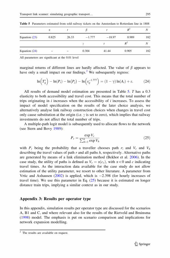
marginal returns of different lines are hardly affected. The value of b appears to

have only a small impact on our findings.2 We subsequently regress:

ln T�ij

� �� ln Pið Þ � ln Pj

� �� ln s�1:777

ij

� �¼ 1� cð Þ ln Aið Þ þ e: ð24Þ

All results of demand model estimation are presented in Table 5. T has a 0.3

elasticity to both accessibility and travel cost. This means that the total number of

trips originating in i increases when the accessibility of i increases. To assess the

impact of model specification on the results of the later choice analysis, we

alternatively analyse link railway construction choices when changes in travel cost

only cause substitution at the origin (i.e. c is set to zero), which implies that railway

investments do not affect the total number of trips.

A multiple-path logit model is subsequently used to allocate flows to the network

(see Stern and Bovy 1989):

Pr ¼expVrPnh¼1 expVh

ð25Þ

with Pr being the probability that a traveller chooses path r; and Vr and Vh

describing the travel values of path r and all paths h, respectively. Alternative paths

are generated by means of a link elimination method (Bekhor et al. 2006). In the

case study, the utility of paths is defined as Vr ¼ aðcrÞ; with a\0 and c indicating

travel times. As the interaction data available for the case study do not allow

estimation of the utility parameter, we resort to other literature. A parameter from

Vrtic and Axhausen (2002) is applied, which is -2.398 (for hourly increases of

travel time). We use this parameter in Eq. (25) because it is estimated on longer

distance train trips, implying a similar context as in our study.

Appendix 3: Results per operator type

In this appendix, simulation results per operator type are discussed for the scenarios

A, B1 and C, and where relevant also for the results of the Rietveld and Bruinsma

(1998) model. The emphasis is put on scenario comparison and implications for

network expansion modelling.

Table 5 Parameters estimated from sold railway tickets on the Amsterdam to Rotterdam line in 1888

a t b t R2 N

Equation (23) 0.825 26.33 -1.777 -18.97 0.989 182

c t R2 N

Equation (24) – – 0.304 41.44 0.905 182

All parameters are significant at the 0.01 level

2 The results are available on request.


123

In Fig. 9, the lengths of the state-built network in the scenarios discussed are

shown as shares of total network length. From the results, it is clear that, in contrast

to the historically built network, all networks modelled obtain a much smaller share

of state-built links. Larger values of / result in larger state involvement, presumably

because potential investments with good return on investment are depleted faster.

The very early onset of state involvement in the historically built network is

0

25

50

0 10 20 30 40 50 60 70 80

Shar

e of

stat

e-bu

ilt n

etw

ork

in m

odel

led

netw

ork

leng

th


Historic net Scenario A Scenario B1 Scenario C

Fig. 9 Shares state-built network length in total network length

0

10

20

30

40

50

60

0 500 1,000 1,500 2,000 2,500

emi tlevart

nirorree gatnecr ep

naeM



Fig. 10 Mean percentage error in travel time on regular private railway lines


123

particularly striking. State involvement was relatively early because network

expansion in the study area was particularly slow at the start (see Veenendaal 1995).

This was the case either because of market imperfections left out of consideration,

or because of the almost exclusive reliance of the transport network on passenger

transport that yielded poor absolute revenues.

Figures 10, 11 and 12 show the mean errors in travel time when only considering

the networks built for regular private lines, state lines and local private lines,

0

10

20

30

40

50

60

0 500 1,000 1,500 2,000 2,500

Mea

n pe

rcen

tage

err

or in

trav

el �

me


Scenario A Scenario B1 Scenario C

Fig. 11 Mean percentage error in travel time on state-built lines

0

10

20

30

40

50

60

0 500 1,000 1,500 2,000 2,500

Mea

n av

erag

e pe

rcen

tage

err

or in

trav

el �

me


Scenario A Scenario B1 Scenario C

Fig. 12 Mean percentage error in travel time on local private lines


123

respectively. The travel times on the subnets are compared with similar subnets of

the historically built network in which the total reference network is about as long as

the total network modelled. Thus, the demonstrated mean errors reflect both

discrepancies in shares per operator type and errors in travel times modelled. From

these results, it is clear that the scenarios B1 and C are the best performers, thus

leading to the conclusion that a value of u of at least five has been obtained by the

railways. When comparing the different operator types, the population-weighted

errors presented here mostly reflect the transport relevance of the various operator

types. Regular private lines served the largest cities, and network allocation errors

on the regular private networks consequently cause emphasized relative errors. In

contrast, the errors on state and local lines have a much lower weight.

Appendix 4: Nomenclature

Ai Interaction options at the origin (destination accessibility)

Alternative Potential addition to the network represented by a link

Base Network before introduction of modelled transport mode or characteristic of existing

transport mode

Bj Interaction options at the destination (origin accessibility)

C Construction costs of link or segment

c Generalized travel cost of link or segment

cp Penalty for entering and exiting the introduced transport mode

curr Network state at start of model iteration

est(x) Estimated network state with treated investment choice in place (multiple versions

indicated by x)

i Origin municipality

INEQACC Changes in the Theil’s index of accessibility due to a considered investment option

intr Characteristic of introduced transport mode

Investor Agent deciding on investments and obtaining revenues from the investment

j Destination municipality

k Parameter used while iterating plausible paths with changing importance of path length

L Length of link or segment

Link (l) Connection between two municipalities (i and j) physically represented by a path

MS Market saturation of i or j, computed as potential number of trips to be gained from link

connection given the current and future network state

Operator Agent deciding on investments and obtaining revenues from the investment

Option Potential addition to the network represented by a link, considered for investment by an

investor

P Municipal population

Path Combination of segments that forms the physical representation of an alternative

R Crudely estimated revenues of a link or segment, instrumental in the generation of plausible

paths, computed by averaging connected population multiplied with MS

RC Revenue-cost indicators per segment, instrumental in the generation of plausible paths,

computed as ratio of R versus C


123

RCR Factor to be optimized in choice set generation computed as ratio of estimated increase in

passenger mileage versus the costs of link construction

ROI An alternative’s expected return on investment, computed as the ratio between estimated

transport flows on the investor’s network and the costs of constructing the alternative

Segment

(s)

Individual, unseparable lines from which paths are composed

T Trips between municipalities i and j

V Speed of transport mode

WCE Population-weighted connection error, used as accuracy indicator

WMAPE Population-weighted average errors in travel times between municipalities, used as

accuracy indicator

Z Selection dummy used to obtain a limited set of alternatives in the first step of choice set

generation

B Parameter governing distance-decay model

c Parameter governing transport consumption elasticity to travel cost at the origin

d Parameter governing trip production for each municipality as a fixed effect

# Parameter governing congestion effects at destination on destination attractiveness

/ Parameter indicating relative travel cost decrease offered by introduced transport mode

References

Alonso W (1978) A theory of movements. In: Hansen NM (ed) Human settlement systems: international

perspectives on structure, change and public policy. Ballinger, Cambridge, pp 197–211

Anshelevich E, Dasgupta A, Tardos E, Wexler T (2003) Near-optimal network design with selfish agents.

In: Proceedings of the thirty-fifth annual ACM symposium on theory of computing, ACM, San

Diego, 9–11 June 2003, pp 511–520

Bala V, Goyal S (2000) A noncooperative model of network formation. Econometrica 68(5):1181–1229

Baranzelli C, Jacobs-Crisioni C, Batista F, Castillo CP, Barbosa A, Torres JA, Lavalle C (2014) The

reference scenario in the LUISA platform—updated configuration 2014 towards a common baseline

scenario for EC impact assessment procedures. Report EUR 27019 EN. Publications Office of the

European Union, Luxembourg

Bekhor S, Ben-Akiva ME, Ramming MS (2006) Evaluation of choice set generation algorithms for route

choice models. Ann Oper Res 144(1):235–247

De Rigo D, Corti P, Caudullo G, McInerney D, Di Leo M, San Miguel-Ayanz J (2013) Toward open

science at the European scale: geospatial semantic array programming for integrated environmental

modelling. Geophys Res Abstr 15:13245

De Vries JJ, Nijkamp P, Rietveld P (2001) Alonso’s theory of movements: developments in spatial

interaction modeling. J Geogr Syst 3(3):233–256

De Vries JJ, Nijkamp P, Rietveld P (2002) Estimation of Alonso’s theory of movements by means of

instrumental variables. Netw Spat Econ 2(2):107–126

Dobbin F, Dowd TJ (1997) How policy shapes competition: early railroad foundings in Massachusetts.

Adm Sci Q 42(3):501–529

Doedens A, Mulder L (1989) Een spoor van verandering: Nederland en 150 jaar spoorwegen. Bosch &

Keuning, Baarn

Donaghy KP (2010) Models of travel demand with endogenous preference change and heterogeneous

agents. J Geogr Syst 13(1):17–30

Economides E (1996) The economics of networks. Int J Ind Organ 14(2):673–699

Filarski R, Mom G (2008) Van transport naar mobiliteit: de transportrevolutie 1800–1900. Walburg,

Zutphen


123

Fotheringham AS, O’Kelly ME (1989) Spatial interaction models: formulations and applications. Kluwer,

Dordrecht

Goodchild MF (1977) An evaluation of lattice solutions to the corridor location problem. Environ Plan A

9(7):727–738

Grubler A (1990) The rise and fall of infrastructures. Dynamics of evolution and technological change in

transport. Physica Verlag, Heidelberg

Guevara CA, Ben-akiva ME (2013) Sampling of alternatives in multivariate extreme value (MEV)

models. Transp Res Part B 48(1):31–52

Hilferink M, Rietveld P (1999) Land use scanner: an integrated GIS based model for long term

projections of land use in urban and rural areas. J Geogr Syst 1(2):155–177

HSM (1889) Financieel verslag over dienstjaar 1888. Metzler & Basting, Amsterdam

Jacobs-Crisioni C, Batista e Silva F, Lavalle C, Baranzelli C, Barbosa A, Castillo CP, Perpina Castillo C

(2016) Accessibility and territorial cohesion in a case of transport infrastructure improvements with

endogenous population distributions. Eur Transp Res Rev 8(9):1–16

Knick Harley C (1982) Oligopoly agreement and the timing of American railroad construction. J Econ

Hist 42(4):797–823

Kolars J, Malin HJ (1970) Population and accessibility: an analysis of Turkish railroads. Geogr Rev

60(2):229–246

Koopmans C, Rietveld P, Huijg A (2012) An accessibility approach to railways and municipal population

growth, 1840–1930. J Transp Geogr 25(1):98–104

Kossmann EH (1986) De lage landen 1780–1980: Twee eeuwen Nederland en Belgie. Elsevier,

Amsterdam

Levinson D, Karamalaputi R (2003) Induced supply: a model of highway network expansion at the

microscopic level. J Transp Econ Policy 37(3):297–318

Levinson D, Xie F (2011) Does first last? The existence and extent of first mover advantages on spatial

networks. J Transp Land Use 4(2):47–69

Levinson D, Xie F, Oca NM (2012) Forecasting and evaluating network growth. Netw Spat Econ

12(2):239–262

Li G, Reis SDS, Moreira AA, Havlin S, Stanley HE, Andrade JS (2010) Towards design principles for

optimal transport networks. Phys Rev Lett 104(018701):1–4

McFadden D (1974) Conditional logit analysis of qualitative choice behavior. In: Zarembka P (ed)

Frontiers in econometrics. Academic Press, New York, pp 105–142

Morrill RL (1970) The spatial organization of society. Duxbury Press, Belmont

Nakicenovic N (1995) Overland transportation networks: history of development and future prospects. In:

Batten D, Casti J, Thord R (eds) Networks in action. Springer, Heidelberg, pp 195–228

ObjectVision (2014) Geo data and model server (GeoDMS). http://objectvision.nl/geodms. Accessed 30

Mar 2016

Patriksson M (2008) Robust bi-level optimization models in transportation science. Philos Trans R Soc A

366(1872):1989–2004

Patuelli R, Arbia G (2013) Editorial: advances in the statistical modelling of spatial interaction data.

J Geogr Syst 15(3):229–231

Rietveld P, Bruinsma F (1998) Is transport infrastructure effective?. Springer, Berlin

Rodrigue J-P, Comtois C, Slack B (2006) The geography of transport systems, 2nd edn. Routledge,

London

Scaparra M, Church R, Medrano FA (2014) Corridor location: the multi-gateway shortest path model.

J Geogr Syst 16(3):287–309

Sen A, Soot S (1981) Selected procedures for calibrating the generalized gravity model. Pap Reg Sci

Assoc 48(1):165–176

Stationsweb (2009) Information on stations in the Netherlands. http://www.stationsweb.nl. Accessed 5

May 2016

Stern E, Bovy PHL (1989) Theory and models of route choice behaviour. Research Institute of Urban

Planning and Architecture, Delft

Taaffe EJ, Morrill RL, Gould PR (1963) Transport expansion in underdeveloped countries: a comparative

analysis. Geogr Rev 53(4):503–529

Veenendaal AJ (1995) State versus private enterprise in railway building in the Netherlands, 1838–1938.

Bus Econ Hist 24(1):186–193

Veenendaal AJ (2008) Spoorwegen in Nederland, 2nd edn. Boom, Amsterdam


123

http://objectvision.nl/geodms

http://www.stationsweb.nl

Vitins BJ, Axhausen KW (2009) Optimization of large transport networks using the ant colony heuristic.

Comput Civ Infrastruct Eng 24(1):1–14

Vrtic M, Axhausen KW (2002) The impact of tilting trains in Switzerland: A route choice model of

regional- and long distance public transport trips. Institut fur Verkehrsplanung und Transportsys-

teme, ETH Zurich, Zurich

Warntz W (1966) The topology of a socio-economic terrain and spatial flows. Pap Reg Sci Assoc

17(1):47–61

Xie F, Levinson DM (2007) Jurisdictional control and network growth. Netw Spat Econ 9(3):459–483

Xie F, Levinson D (2009) Modeling the growth of transportation networks: a comprehensive review.

Netw Spat Econ 9(3):291–307

Xie F, Levinson D (2011) Evolving transportation networks. Springer, New York

Youn H, Gastner MT, Jeong H (2008) The price of anarchy in transportation networks: efficiency and

optimality control. Phys Rev Lett 101(128701):1–4


123

Transport link scanner: simulating geographic transport · PDF filetransport network expansion...

Documents

Transcript of Transport link scanner: simulating geographic transport · PDF filetransport network expansion...