1

NUMERICAL SIMULATION OF TRANSONIC

FLOW OVER 3D WING

A Progress Report

Submitted in Partial Fulfillment of the Requirements for the

Degree of

MASTER OF TECHNOLOGY

(AEROSPACE & APPLIED MECHANICS)

(Specialization: Mechanics of fluid)

BY

CHANDAN KUMAR

EXAMINATION ROLL NO.: 321315001

REGISTRATION NO.: IIEST151600775

Of YEAR 2015-2016

Under the guidance of

DR. SUBHASIS BHAUMIK

DEPARTMENT OF AEROSPACE ENGINEERING

& APPLIED MECHANICS

INDIAN INSTITUTE OF ENGINEERING SCIENCE AND TECHNOLOGY,

SHIBPUR

2

DEPARTMENT OF AEROSPACE & APPLIED MECHANICS

INDIAN INSTITUTE OF ENGINEERING SCIENCE AND TECHNOLOGY,

SHIBPUR

FORWARDING

I hereby forward the thesis report entitled “NUMERICAL SIMULATION OF

TRANSONIC FLOW OVER 3D WING” submitted by CHANDAN

KUMAR(Roll No.-321315001) under my guidance and supervision in partial

fulfillment of the requirements for the degree of ‘Master of Technology’ in

Mechanics of Fluids in the Department of Aerospace Engineering & Applied

Mechanics, Indian Institute of Engineering Science and Technology, Shibpur.

Dated……. /...……/……….……

(Dr. S. BHAUMIK) Professor & Head

Department of Aerospace Engg. & Applied Mechanics

Indian Institute of Engineering Science and Technology

Shibpur, Howrah-711103, WB

COUNTERSIGNED BY:

………………………………

…………………………………

(Dr.S.BHAUMIK)

Professor & Head Dean(Academics) Dept. of Aerospace Engg. & Applied Mechanics Indian Institute of Engg Science Indian Institute of Engg Science & Tech, Shibpur & Tech, Shibpur

3

DEPARTMENT OF AEROSPACE & APPLIED MECHANICS

INDIAN INSTITUTE OF ENGINEERING SCIENCE AND TECHNOLOGY

SHIBPUR

HOWRAH- 711103

CERTIFICATE OF APPROVAL

The foregoing report is hereby approved as a creditable study of Engineering subject carried out

and presented in a satisfactory manner to warrant its acceptance as a prerequisite for the Degree

of ‘Master of Technology’ in Aerospace & applied mechanics (Mechanics of Fluids) in the

Department of Aerospace Engineering & Applied Mechanics, Indian Institute of Engineering

Science and Technology, Shibpur for which it has been submitted. It is understood that by this

approval the undersigned do not necessarily endorse or approve any statement made, opinion

expressed or conclusion drawn therein but approve the report only for the purpose for which it is

submitted.

Board of Thesis Examiners:

1.…………………………………….

2.…………………………………….

3.…………………………………….

4

ACKNOWLEDGEMENT

I take this opportunity to express my sincere thanks to my thesis guide, Dr. S.Bhaumik,

Department of Aerospace Engg. & Applied Mechanics of Indian Institute of Engineering Science

and Technology, Shibpur for his invaluable guidance, advice, constant encouragement and

enlightening discussions during the course of this research work without which it would not have

been possible for me to give the progress report in this shape.

Dated:……………………….

(CHANDAN KUMAR)

Examination Roll No.-321315001

Indian institute of Engineering Science and Technology, Shibpur

Howrah: 711103

5

TABLE OF CONTENTS

Chapter Page

1. INTRODUCTION…………………………………………………6

1.1 Background……………………………………………………6

1.2 Objective……………………………………………………….7

2. LITERATURE REVIEW………………………………………….8

3. NUMERICAL SIMULATION…………………………………….9

3.1 Modeling……………………………………………………….9

3.2 Meshing………………………………………………………..15

3.3 Analysis………………………………………………………..16

4. RESULTS AND DISCUSSION…………………………………..20

4.1 Convergence…………………………………………………...20

4.2 Results and comparison……………………………………....23

4.2.1 Lift and Drag verification……………………………….26

4.2.2 Pressure verification…………………………………….27

5. CONCLUSION AND FUTURE WORK………………………...30

5.1 Conclusion…………………………………………………….30

5.2 Future work…………………………………………………...30

REFERRENCE…………………………………………………………31

6

1. INTRODUCTION

1.1 Background

The transonic regime is a critical range of flight that has been widely studied from the

1930s. The vast majority of air transports operate in this regime. Similarly, fighter and strike

aircraft, despite being capable of supersonic flight, tend to operate in the transonic range. There

are numerous factors that affect transonic fight such as shock wave and turbulence boundary-

layer interaction which can induce flow separation and cause large-scale instability.

Experiments have been performed to investigate transonic flow over wing. Modern transonic

wind tunnels that operate at high Reynolds numbers are able to obtain reasonably accurate data

for large transports. Within the past two decades or so, advances in numerical techniques and

computational power have ensured the viability of computational fluid dynamics (CFD) in

studying fluid phenomenon. An interesting development of late is the synergism between

experimental and computational methods. For example, computations may be verified using

existing experimental databases. On other hand, computations have the ability to check

experiments, such as to ensure that wall interference effects are properly taken into account.

Transonic flows signify too many complex phenomena, contact discontinuities, such as creation

of shock, buffet onset and shock-boundary-layer interaction. Since these flows are robustly time-

dependent and cannot be fully implicit without reference to viscous character of the fluid, as

viscous terms are significant in their interaction with the convective process.

In real viscous flows, a change in flow field occurs in non-monotonic trend and leads to surface

instability, even in the absence of unsteady boundary conditions. Therefore, transonic flows must

be illustrated by the time dependent, compressible Navier-Stokes equations. Numerical methods

for solving Navier-Stokes equations must be capable of predicting all the above flow

characteristic accurately. Turbulent shock/boundary-layer interaction adjacent to an airfoil’s

surface has a intensely effect on the aerodynamic performance of a transonic aircraft due to the

rapid thickening of boundary layer induced by the shock.

When the shock is adequately strong to provoke boundary layer separation, a ‘k-shock’ structure

originates close to the separation point. This extensively affects the resulting drags and lift

coefficients. The concurrent presence of high pressure gradient, shear, and recirculation related

curvature close to a solid surface leads to a complex, highly anisotropic turbulence of structure.

Extensive occurrence with such conditions in incompressible flows recommends that advanced

modeling practices, based on second-moment closure, are often essential for a satisfactory

prediction of recirculation.

7

1.2 Objective

The present study deals with the analysis of transonic flow over 3D ONERA- M6 wing.

Aerodynamic characteristic of wing such as static and dynamic pressure, skin friction

coefficient, turbulence intensity in transonic regime the performance parameters of wing

such as angle of attack, lift coefficient, drag coefficient has been analyzed and predicted

with the help of finite volume tool ANSYS-Fluent.

The transonic compressible flow simulation has been carried out using Spalart-Allmaras

turbulence model and PRESTO solution technique has been applied to govern Euler and

Navier-Stokes continuity principle.

The results obtained from finite volume technique are verified with well published in

literature and furthermore with experimentation as per the graph and figure are generated.

This simulation is modeled after the simulation done by NASA using WINDSIM and we

try to produce results here. It is from there we have obtained the experimental data for

comparison purposes.

The research objectives are to verify the experimental data and to confirm the ability of a

commercial flow solver for simulating configuration in a transonic tunnel

8

2. LITERATURE REVIEW

CFD Applications: Transonic airfoils and wings [ JD Anderson] : Modern subsonic transports

such as Boeing 747, 777 etc. cruise at the free stream Mach number on the order of 0.85, and

high-performance military combat air-planes spend time at high subsonic speeds near Mach one.

These airplanes are in the transonic flight regime. The only approach that allows the accurate

calculation of airfoil and wing characteristics at transonic speeds is to use computational fluid

dynamics. The need to calculate accurately the transonic flow over airfoils and wings was one of

the two areas that drove advances in CFD in early days of its development, the other area being

hypersonic flow .Beginning in the 1960s, transonic CFD calculations historically evolved

through four distinct steps as follow;

1. The earliest calculations numerically solved the non-linear small perturbation potential

equation for transonic flow

2. The next step was numerical solutions of the full potential equation. This allowed

applications to airfoils of any shape at any angle of attack. However, the flow was still

assumed to be isentropic, and even though shock wave appeared in the result, the

properties of these shocks were not always accurately predicted.

3. As CFD algorithms became more sophisticated, numerical solutions of the Euler

equations were obtained. The advantage of these Euler solutions was that shock waves

were properly treated

4. This led to the CFD solution of the viscous flow equations( the Navier Stokes equation)

for transonic flow. Such CFD solutions of the Navier stokes equations are currently the

state of the art in transonic flow calculations.

Turbulent Shock-wave/Boundary-layer interaction [AGARD-AG-280, NATO]: In analyzing

flows past obstacles, both from theoretical and a phenomenological point of view, it is customary

to conceptually divide the field into distinct zones consisting of : 1) Regions where viscous

effects play a negligible role. There the flow is said to behave like a perfect fluid which means

that the dissipative effects are inexistent. In these regions, the fluid motion can be accurately

computed by solving the Euler equations. Frequently, the perfect fluid region is called the outer

or external flow field. 2) Regions where viscosity must play a predominant role, namely:

boundary-layers, wakes, mixing zones.

Finite volume method for transonic flow calculation [Antony Jameson CIMS NY]: This paper

explained a method for calculating transonic potential flow which can be applied to bodies of

more or less arbitrary geometric, complexity, given a sufficiently powerful computer. It is

proposed to circumvent the geometric difficulties by deriving a discrete approximation on a

mesh constructed from volume elements which can be conveniently packed around the body.

This leads to a relatively simple treatment of the exact potential flow equation in conservation

form

9

3. NUMERICAL SIMULATION

The numerical approach utilized ANSYS workbench. For designing a 3D wing model

SOLIDWORKS has been used later this is modeled in ANSYS DESIGN MODELER, where the

flow domain has been created. Subsequently ANSYS ICEM CFD meshing was used to generate

unstructured tetrahedral mesh for using in computation. CFD-Post used to generate graph and

flow counters.

3.1 Modeling

The model of this simulation is ONERA-M6 wing half model. For creating the wing first we

need to make the airfoil. We obtained the coordinate for ONERA OA206 airfoil from the

airfoiltools.com. The coordinate has been obtained for 100 points on the upper and lower surface

of airfoil. These coordinates have been imported to solidworks in order to generate the airfoil.

NASA have performed experimental work on the ONERA-M6 on original wing with one side

span of 1.196 meters. So in order performs CFD simulation first we have to scale down

everything.

Our model has been scaled down by factor 3.9 of the model used NASA for their experiment.

Before getting into scaling down the model we have some common terms regarding geometry

that we have to keep in mind. Those terms are as follow.

Terminology

Wing root chord (Cr):- It is the chord of airfoil at root of the aircraft wing.

Wing tip chord (Ct):- It is chord of airfoil at the tip of aircraft wing.

Aspect ratio (AR):- It is ratio of Span Square to the surface area of wing.

𝐴𝑅 =𝑏2

𝑆 ; b = span; S = surface area

Taper ratio: - It is ratio of tip chord and root chord.

Taper ratio = Ct/Cr; for untapered wing Ct=Cr

Mean aerodynamic chord: - It is average of tip chord and root chord.

Cm = (Ct + Cr) / 2

Leading & trailing edge sweep angle: - It is angle made between vertical line and leading edge &

vertical line and trailing edge in 2D plane looking form top.

10

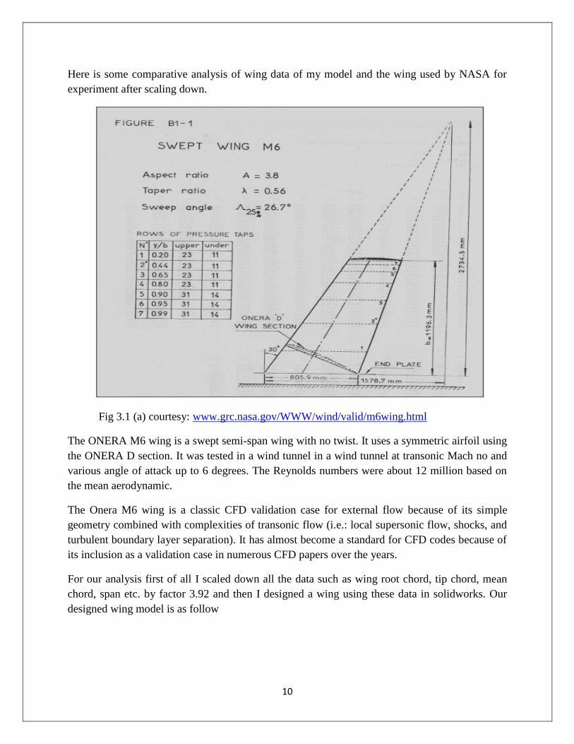
Here is some comparative analysis of wing data of my model and the wing used by NASA for

experiment after scaling down.

Fig 3.1 (a) courtesy: www.grc.nasa.gov/WWW/wind/valid/m6wing.html

The ONERA M6 wing is a swept semi-span wing with no twist. It uses a symmetric airfoil using

the ONERA D section. It was tested in a wind tunnel in a wind tunnel at transonic Mach no and

various angle of attack up to 6 degrees. The Reynolds numbers were about 12 million based on

the mean aerodynamic.

The Onera M6 wing is a classic CFD validation case for external flow because of its simple

geometry combined with complexities of transonic flow (i.e.: local supersonic flow, shocks, and

turbulent boundary layer separation). It has almost become a standard for CFD codes because of

its inclusion as a validation case in numerous CFD papers over the years.

For our analysis first of all I scaled down all the data such as wing root chord, tip chord, mean

chord, span etc. by factor 3.92 and then I designed a wing using these data in solidworks. Our

designed wing model is as follow

11

Fig 3.1 (b) Designed wing model with scale down factor of 3.92

Here is some comparative data of original ONERA-M6 wing and designed wing .

Specification ONERA-M6 wing used

NASA for

Tunnel experiment

Solidworks designed model

For FLUENT analysis

Wing root chord 2.64 ft 0.67 ft

Wing tip chord 1.49 ft 0.38 ft

Taper ratio 0.562 0.562

Mean aerodynamic

chord

2.1 ft 0.53 ft

Half wing span b 3.92 ft 1 ft

Leading edge sweep

angle

300 300

Trailing edge sweep

angle

15.80 15.80

Aspect ratio 3.8 3.8

Wing twist NO NO

12

Airfoil specification

Fig : 3.1 (c) Wing cross section ( airfoil) at root

Symmetry airfoil – means no camber

Chord - 0.67 ft.

Maximum thickness – 0.104 ft. at quarter chord from leading edge.

Trailing edge angle – 19.40 deg.

Since this is symmetry airfoil so the lift will be zero at aero angle of attack. The lift curve slope

has been obtained from the graph at the airfoiltools.com which is as follow

𝑑𝑐𝑙

𝑑𝛼= 0.0884 = 𝑎0

Using this we can calculate the lift curve for finite wing will be using the correction for a swept

wing. We need to use this correction for a swept wing since the free stream Mach no. is not seen

by entire wig and instead the wing sees a lesser Mach no, delaying the onset of a shock and

increasing the critical Mach number. The following formula is used to convert the infinite wing

lift slope to the finite swept wing lift slope.

AR – Aspect ratio

after we use all of our values, we get a corrected slope a = .0760. For finite wings, we know that

the lift curve will be lower than for infinite wings due to 3D effects and this is reflected our

calculation here. Once we know the slope for our finite wing, we can calculate the lift coefficient

for the wing as follow.

13

Since the airfoil is symmetric, we will say that αL = 0. Then, we get that our lift coefficient is

.2328. However, this is for the entire wing (remember that we use only half for our simulation)

and the data that we used to calculate this is for low speed incompressible flows. This means that

we need to use a correction for the compressibility at M = .8395.

Using this correction factor, we get that the lift coefficient for the entire wing will be .4284.This

would be for the entire wing and for our half wing, we simply divide by 2 to predict a lift

coefficient of .2141.

Importing of solidworks geometry file to ANSYS workbench & domain formation

The wing geometry which was created in solidworks has been imported to ANSYS-Fluent. In

order to capture the flow around the wing, suitable domain has been created using tools available

in workbench. The following figure shows the domain surrounding the wing with a near side

contacting the wing surface.

Fig: 3.1(d) Flow domain around wing

The above figure is showing the domain for half of the wing span , in which the wing surface

acts as wall, near side is symmetry whereas the other boundary are inlet , outlet & far field on

which we need to specify pressure, Mach no. temperature and component of velocity .

14

Boundary condition

Boundary Name Boundary Type Condition

Near_side Symmetry Symmetry w.r.t boundary

Wing_surface Wall V = 0

Inlet,

Far_side

Outlet

Pressure far-field P = 45.82 psia = 2.11 atm

T = 460 R = 255.5 k

M = 0.839

Angle of attack = 3.06 deg

Reynolds no. 11.72E6

Side slip angle = 0

Density = Ideal gas

Viscosity = 1.09329E-5 lbm/ft-s

2.2 Meshing

ANSYS MESHING was used to generate an unstructured mesh for the computations. The

unstructured mesh consisted of small tetrahedral grid near to the area of interest namely wing

and larger sizes further away. This mesh distribution yielded accuracy and allows for complex

gradients around the wing to be resolved for a minimum number of meshes.. The final process of

meshing is to define the boundary conditions for the model.

Fig: 3.2 (a) 3D Unstructured Meshed domain (b) Finer mesh near the wing body

15

Tetrahedral mesh has triangular structure in 2D plane. Mesh quality can be judge by the

orthogonal quality of mesh. The orthogonal quality value varies from 0 to 1. In case here

minimum orthogonal quality of mesh is 7.976e-2. Another term we define is that aspect ratio of

mesh.

Aspect ratio for triangular grid = 2Ri/ Ro

Where Ri = Radius of circle inscribed in triangle

Ro = Radius of circle circumscribed circle around triangle

Mesh summary

Mesh structure Tetrahedral

No. of nodes 1,01,063

No. of elements 3,69,052

Minimum

orthogonal quality

7.92 e-2

Aspect ratio 3.162e+2

Fig 3.2 (c) Wing body finely meshed at leading and trailing edge to capture the flow

Wing has been meshed finely at leading and trailing edge. In transonic flow condition there is

formation of sonic pocket over the wing and also there is interaction between shock and

boundary layer so this requires finer meshing compare to other parts of the wing.

16

2.3 Analysis

Here we come to the analysis part where we import the meshed file to the FLUENT solver.

Problem is solved with density based and steady option. Since here our flow condition is

turbulent so we have used the Spalart-Allmaras turbulence model

Our simulation is governed by Continuity, Momentum (Navier-Stokes) , energy equation. But

since this is turbulent flow so we will be using Reynolds Averaged version of this equations. The

equations are as follow

Law of conservation of mass (Continuity equation):

Differential form

where

ρ is fluid density,

t is time,

u is the flow velocity vector field

By Reynolds decomposition we can write the instantaneous flow velocity as the sum of

averaged and fluctuation velocity as follow

So we can now write for steady, incompressible flow as

On Reynolds time averaging this equation we get

17

Hence the Reynolds averaged continuity equation can be written for unsteady,

compressible flow as

Law of conservation of Momentum (Navier-Stokes equation):

From Momentum equation the Navier-Stokes equation can be written as

On replacing the instantaneous variable with the sum of averaged and fluctuation term and

then averaging it we get Reynolds averaged Navier-Stokes equation as follow

where, mean strain rate tensor is given by

On comparing Navier-Stokes equation with RANS we found that there is one extra term in

RANS that is Reynolds stress tensor

Law of conservation of Energy ( Energy equation):-

Energy equation can be drived based on First law of thermodynamics which is given as

follow

18

In fluid dynamics, turbulence kinetic energy (TKE) is the mean kinetic energy per unit

mass associated with eddies in turbulent flow. Physically, the turbulence kinetic energy is

characterized by measured root-mean-square (RMS) velocity fluctuations.

In Reynolds-averaged Navier-Stokes equations, the turbulence kinetic energy can be

calculated based on the closure method, i.e. a turbulence model. The full form of TKE

equation can be given as follow:

Where, k is the mean of turbulence normal stresses given by

Spalart Allmaras Turbulence modeling

The Spalart–Allmaras model is a one-equation model that solves a modeled transport

equation for the kinematic eddy turbulent viscosity. The Spalart-Allmaras model was

designed specifically for aerospace applications involving wall-bounded flows and has been

shown to give good results for boundary layers subjected to adverse pressure gradients. It is

also gaining popularity in turbo machinery applications.

In its original form, the Spalart-Allmaras model is effectively a low-Reynolds number

model, requiring the viscosity-affected region of the boundary layer to be properly resolved (

y+ ~1 meshes). In ANSYS-FLUENT, the Spalart-Allmaras model has been extended with a

y+ -insensitive wall treatment (Enhanced Wall Treatment), which allows the application of

the model independent of the near wall y+ resolution.

The formulation blends automatically from a viscous sub layer formulation to a logarithmic

formulation based on y+. On intermediate grids, (1< y+ <30), the formulation maintains its

integrity and provides consistent wall shear stress and heat transfer coefficients. While the y+

sensitivity is removed, it still should be ensured that the boundary layer is resolved with a

minimum resolution of 10-15 cells.

Spalart Allamaras Turbulence model is given by

Where Sij is strain rate tensor given by

19

The Spalart-Allmaras model has only one equation which solves for the kinematic eddy

viscosity. We need to solve for the variables of the problem in all cell centers of our mesh. In

total, we have six variables to solve for: 3 components of velocity, pressure, temperature, and the

kinematic eddy viscosity.

20

4. RESULTS AND DISCUSSION

The equations are converted to algebraic equations. It then solves for our six variables at each of

the cell centers of our mesh. This means that if we have 300,000 cells, FLUENT is going to

solve 1.8 million equations to solve the problem.

In this simulation, we expect to see many flow features in three dimensions. We will be

especially interested in the suction peak (low pressure zone) that forms on the wing and how the

size of the suction peak changes spanwise. We will also be looking for a shock along the wing

surface as this is transonic flow. We also expect to see trailing edge vortices forming

downstream of the wing, due to the interaction of the high and low pressure zones since this is a

finite length wing.

4.1 Convergence

There are no universal metrics for judging convergence. Residual definitions that are useful for

one class of problem are sometimes misleading for other classes of problems. Therefore it is a

good idea to judge convergence not only by examining residual levels, but also by monitoring

relevant integrated quantities such as drag or heat transfer coefficient.

Generally at convergence following condition should be satisfied

All discrete conservation equations (momentum, energy, etc.) are obeyed in all cells to a

specified tolerance OR the solution no longer changes with subsequent iterations.

Overall mass, momentum, energy, and scalar balances are achieved.

Generally, a decrease in residuals by three orders of magnitude indicates at least qualitative

convergence. At this point, the major flow features should be established.

Scaled energy residual should decrease to 10-6 (for the pressure-based solver).

Scaled species residual may need to decrease to 10-5 to achieve species balance.

Monitoring quantitative convergence:

Monitor other relevant key variables/physical quantities for a confirmation.

Ensure that overall mass/heat/species conservation is satisfied.

In addition to residuals, we can also monitor lift, drag and moment coefficients. Relevant

variables or functions (e.g. surface integrals) at a boundary or any defined surface. In addition to

monitoring residual and variable histories, we should also check for overall heat and mass

balances. The net flux imbalance should be less than 1% of the smallest flux through the domain

boundary. If solution monitors indicate that the solution is converged, but the solution is still

changing or has a large mass/heat imbalance, this clearly indicates the solution is not yet

converged.

Here the simulations were defined to investigate the converged solution by monitoring the

residuals of continuity, velocity components, energy, and eddy viscosity. Convergence criteria

were determined when the residual were less than 0.001. The maximum iteration was set to 1000

in order to observe that the solution was converged, and the simulations automatically proceeded

to the final step of iteration. In addition, lift and drag coefficients were monitored for examining

21

the converged solution. The results are shown here. These figures show that convergence was

achieved at about 190 iteration.

Fig 4.1 The iterations for the residual of continuity, velocity components, energy & eddy

Fig 4.2 The iteration of lift convergence history at M = 0.839 and α = 3.060

22

Fig 3.3 The iteration of lift convergence history at M = 0.839 and α = 3.060

4.2 Result and comparison

This part includes the various plots and contour of different variables. Since we are dealing

with transonic flow, the flow will supersonic at some location over the wing. The pressure at

leading edge will be higher due to conversion from kinetic to pressure energy. As flow start

to move downstream it will start accelerate and achieve sonic velocity at some point which

leads to formation of shock wave over wing. After the shock wave there is sudden increase

in pressure. The following figure show the variation of pressure along the wing span

Fig 4.4 Variation of pressure coefficient over the surface of wing at M=0.839 and α =3.06

23

From the above figure it can be clearly seen that at root of wing pressure increases suddenly at

approx.. 2/3rd of chord from leading edge whereas this happen at tip at 1/4 th of chord from

leading edge. Similarly pressure contour variation over wing has been obtained shown as follow

Fig: 4.5 Pressure contour lines at root and tip of the Onera-M6 wing

On comparing the above pressure contour lines it can be clearly seen that the sudden increase in

pressure is much closer to leading edge at tip in compared to the root. This explains that there is

shock wave near leading at the tip of wing

Since the free stream Mach no. is transonic, the flow will achieve Mach 1 over the wing and it

leads to formation of shock, which interacts with the boundary layer formed over the surface.

This phenomenon is one of the most interested topic for scientist and engineers called as Shock-

Boundary Layer interaction. This process cause the local heating of the wing surface

Basically a boundary layer is a thin layer across which the flow velocity decreases from high

external value to zero at the wall where the no-slip condition must be satisfied. At the same time,

the Mach number varies from the outer value M∞ to zero. Since the static pressure is

transversally constant across it, the boundary-layer can be viewed as a quasi-parallel flow with

variable entropy from one streamline to the other, or which is equivalent, as a quasi-parallel

rotational flow

Here we have obtained the clear Mach number contour variation along the cross section of wing

at the root.

24

Fig: 4.6 Mach contour lines at the root of the wing having shock along with boundary layer

When a shock-wave propagates through a boundary-layer, it sees an upstream flow of lower and

lower Mach number as it approaches the wall. The shock must adapt itself to this situation so that

it becomes vanishingly weak when it reaches the place where the Mach number is sonic.

Moreover, the pressure signal carried by the shock is necessarily transmitted in the upstream

direction through the subsonic inner part of the boundary-layer. Thus the pressure rise caused by

the shock is felt upstream of the point where the shock would meet the surface in a flow without

boundary layer.

The transfer of momentum caused by turbulent eddies is often modeled with an effective eddy

viscosity in a similar way as the momentum transfer caused by molecular diffusion is modeled

with a molecular viscosity. The hypotheses that effect the turbulent eddies on the flow can be

modeled in this are often referred to as the Boussinesq eddy viscosity assumption. Flow over the

wing here is turbulent so there is existence of eddy viscosity.

Fig: 4.7 Eddy viscosity strength contour lines at the root and tip of the wing

25

Fig: 4.8 After effect of eddies generating from wing placed in M = 0.839

The eddies generated from the wing in transonic flow exist longer behind the wing and effect the

performance of the aircraft. So this must be reduced in the proper manner to reduce the drag.

This eddies are more severe at the wing tip as shown above which leads to sharp reduction in the

lift at the wing tip.

In order to look at the velocity vector at the trailing edge of the wing we create a vertical plane at

the trailing edge of the wing. This plane is facing the free stream of the flow coming through the

wing.

Fig: 4.9 Plane generated at the trailing edge of the wing and velocity vector leaving trailing edge

26

Fig:4.10 Front view of velocity vector leaving trailing edge

In the above figure it can be seen clearly that most of the velocity vector are perpendicular to the

plane but near the wing tip these velocity vector is no longer perpendicular , it got tilted and

having the circular motion causing wing tip vortices.

Vortices form because of the difference in pressure between upper and lower surfaces of a wing

that is operating at a positive lift. Since pressure is a continuous function, the pressure must

become equal at wing tips. The tendency is for particles of air to move from the region of high

pressure to the region of low pressure so that the pressure becomes equal above and below the

wing. In addition, there is an inclined inward flow of air on the upper wing surface and an

inclined outward flow of air on the lower wing surface. The flow is strongest at the wing tips and

decreases to zero at the midspan (wing-root) as evidence by the flow direction there being

parallel to the free-stream direction.

4.2.1 Lift and drag verification

Lift Force – Direction Vector ( -0.0534 0.9986 0)

Forces

(lbf)

Force

Coefficients

Zone Pressure Viscous Total Pressure viscous Total

Wing_surface 439.2911 -0.2633 439.0277 0.12548 -7.52e-05 0.1254

Wing_tip -1.2e-07 0.0138 0.01384 -3.42e-11 3.95e-06 3.95e-06

Net 439.2911 -0.2495 439.0415 0.12548 -7.12e-05 0.1254

27

Drag Force – Direction Vector (0.9986 0.0534 0)

Forces

(lbf)

Force

coefficients

Zone Pressure Viscous Total Pressure Viscous Total

Wing_surface 30.4809 8.0124 38.4933 0.0087 0.0022 0.01099

Wing_tip 3.84e-07 0.09061 0.09061 1.09e-10 2.58e-05 2.58e-05

Net 30.4809 8.1030 38.5839 0.00870 0.00231 0.01102

Comparison with NASA CFD

We compared the drag and lift coefficient to those from NASA’s WIND simulation:

Lift Coefficient

CL

Drag Coefficient

CD

Percent

Difference CL

Percent Difference

CD

NASA CFD 0.1410 0.0088 …… ……

Original Mesh 0.1254 0.01102 11.06 22.2

Refined Mesh 0.1302 0.0090 8.42 12.6

For refined mesh the relevance factor has been increased from zero to fifty with the leading edge

face and trailing edge face cell sizes further refined. Relevance center has been changed from

coarse to medium. Smoothing of the mesh sizing selected as medium to get refined mesh.

4.2.2 Pressure variation verification

We ran the simulation and compared the pressure variation over the wing with the existing data

available on NASA website http://www.grc.nasa.gov/WWW/wind/valid/m6wing.html and graph

has been plotted using CFD-POST.

28

Fig: 4.11 comparison of variation of Cp on top and bottom surface at y/b = 0.2

Fig: 4.12 Comparison of variation of Cp on top and bottom at y/b = 0.44

29

Fig: 4.13 Comparison of variation of Cp on top and bottom surface at y/b = 0.65

30

5. CONCLUSION AND FUTURE WORK

5.1 Conclusion

Numerical simulations are presented for the flow over Onera-M6 wing in the transonic

regime. The computation were performed for mesh having number of nodes 1,01,063.

The three dimensional simulations were conducted for a half wing. Aerodynamic data

such as pressure distributions and lift and drag coefficient were obtained and compared

with existing data.

The shock wave formed over the wing is closer to leading edge at the wing tip compared

to wing root. This predicts that the flow will separate earlier at the wing tip and there is

loss in lift.

The comparison experimental and fluent result showed discrepancies in regions of

shock/boundary-layer interactions. Despite this, the overall lift and drag coefficient

appeared to compare well with experimental result

5.2 Future work

To run the simulation at different Mach number in transonic regime varying form 0.8 to

1.2 and to observe the location of shock wave

To obtain the lift coefficient curve at different location of span leading from wing root to

wing tip.

To check the variation in lift and drag forces with the shift of maximum thickness of

airfoil towards the trailing edge.

Despite the difficulty in resolving regions with shock/boundary-layer interaction, the

numerical simulation appeared to be suitable for studying transonic aerodynamics. Future

work will be also extended to more realistic wing having supercritical airfoil.

31

REFERENCE

[1] Peter M. Goorjian, Guru P. Guruswamy, “Transonic unsteady aerodynamic and aeroelstic

calculations about airfoils snad wings”,Computers & structures, Vol 30, Issue 4,1988, page 929-

936

[2] Angelo Iollo, Manuel D. Salas,”Optimum transonic airfoils based on Euler equations”,

Computers and Fluids, Vol 28, Issues 4-5, May-June 1999

[3] Jose L. Vadillo, Ramesh K. Agarwal, Ahmed A. Hasan, “Active Control of Shock/Boundary

layer interaction in Transonic flow Over airfoils”, Copmutational Fluid Dynamics 2004 2006,pp

361-366

[4] “CFD Applications: Transonic airfoils and wings” Jhon D Anderson , fifth edition page 729

[5] Tapan K. Sengupta, Ashish Bhole, N.A. Sreejith, “Direct numerical simulation of 2D

transonic flows around airfoils”, Computers & Fluids , Volume 88,15 dec 2013 page 19-23

[6] “Shock-Wave Boundary Layer interactions” Advisory group for aerospace research &

development. AGARD-AG-280

[7] W. C. Selerowicz,”Prediction of transonic wind tunnel test section geometry-a numerical

study”’ The archive of mechanical engineering, vol. LVI,pp. 113-130, 2009