Transmitting and Gathering Streaming Data in Wireless Multimedia Sensor Networks within Expected...
40
Transmitting and Gathering Streaming Data in Wireless Multimedia Sensor Networks within Expected Network Lifetime Lei Shu Yan Zhang Digital Enterprise Research Institute Simula Research Laboratory [email protected] [email protected]
-
Upload
darcy-morton -
Category
Documents
-
view
223 -
download
0
Transcript of Transmitting and Gathering Streaming Data in Wireless Multimedia Sensor Networks within Expected...
Transmitting and Gathering Streaming Data in Wireless
Multimedia Sensor Networks within Expected Network
Lifetime Lei Shu Yan Zhang
Digital Enterprise Research Institute Simula Research Laboratory
Wireless Sensor NetworksDigital Enterprise Research
Institute
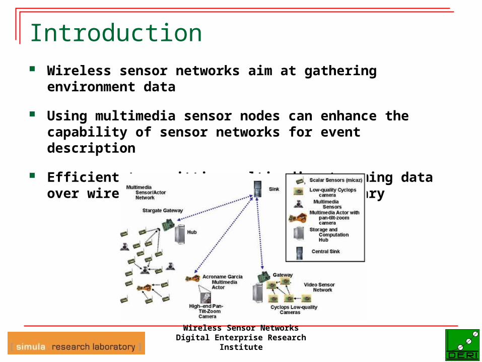
Introduction Wireless sensor networks aim at gathering
environment data
Using multimedia sensor nodes can enhance the capability of sensor networks for event description
Efficient transmitting multimedia streaming data over wireless sensor networks is necessary
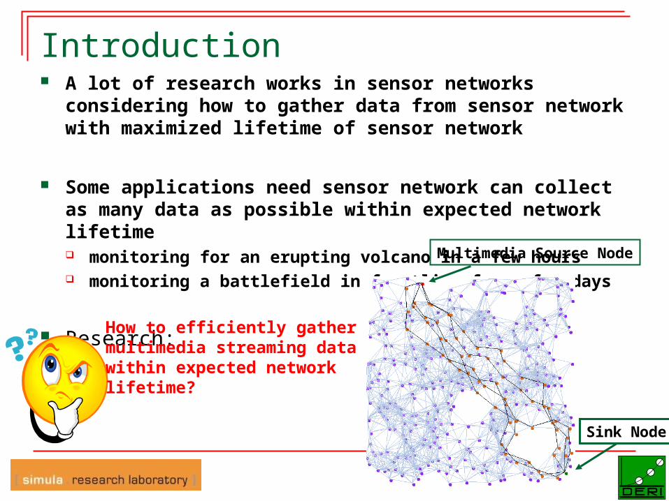
Introduction A lot of research works in sensor networks
considering how to gather data from sensor network with maximized lifetime of sensor network
Some applications need sensor network can collect as many data as possible within expected network lifetime monitoring for an erupting volcano in a few hours monitoring a battlefield in frontline for a few days
Research:
Multimedia Source Node
Sink Node
How to efficiently gather multimedia streaming data within expected network lifetime?
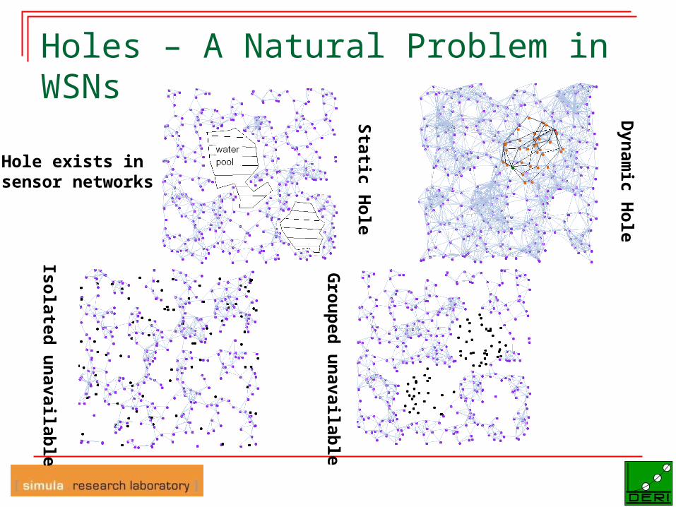
Holes – A Natural Problem in WSNs
Sta
tic
Hole
Dyn
am
ic
Hole
Isola
ted
u
nava
ilab
le
Gro
up
ed
u
nava
ilab
le
Hole exists in sensor networks
Requirements on Multimedia Streaming Shortest path transmission
Multimedia applications generally have a delay constraint which requires that the multimedia streaming in WSNs should always use the shortest routing path which has the minimum end to end transmission delay.
Multipath transmission Packets of multimedia streaming data generally are
large in size and the transmission requirements can be several times higher than the maximum transmission capacity (bandwidth) of sensor nodes.
Hole-bypassing Dynamic holes may occur if several sensor nodes in a
small area overload due to the multimedia transmission.
State-of-the-art (1) Existing Data Gathering Problem in WSNs
Maximum lifetime data gathering Balance data gathering Maximum data gathering
No research work has ever considered “ Streaming Data Gathering in Wireless Multimedia S
ensor Networks within Expected Lifetime”
State-of-the-art (2) E. Gurses, O. B. Akan, Multimedia Communication in
Wireless Sensor Networks, in Annals of Telecommunications, vol. 60, no. 7-8, pp. 799-827, July-August 2005.
I. F. Akyildiz, T. Melodia, and K. R. Chowdury, “A Survey on Wireless Multimedia Sensor Networks,” Computer Networks (Elsevier), Vol. 51, no. 4, pp.921-960, March 2007.
Existing protocols from both multimedia and sensor networks fields are not suitable for multimedia communication in wireless sensor networks
No solution proposal specifically tailored to address the routing problems of multimedia streams in wireless sensor networks
State-of-the-art (3) Limited research work had been done for
hole bypassing routing
Two catagories Hole bypassing without knowing hole information
in advance GPSR Destination’s location information 1-hop neighbor nodes’ location information
Hole bypassing with hole information & boundary nodes information in advance Destination’s location information 1-hop neighbor nodes’ location information Boundary nodes information & hole information
Holes and their boundary nodes can be identified in advance
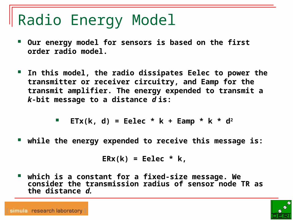
Radio Energy Model Our energy model for sensors is based on the first order
radio model.
In this model, the radio dissipates Eelec to power the transmitter or receiver circuitry, and Eamp for the transmit amplifier. The energy expended to transmit a k-bit message to a distance d is:
ETx(k, d) = Eelec * k + Eamp * k * d2
while the energy expended to receive this message is:
ERx(k) = Eelec * k,
which is a constant for a fixed-size message. We consider the transmission radius of sensor node TR as the distance d.
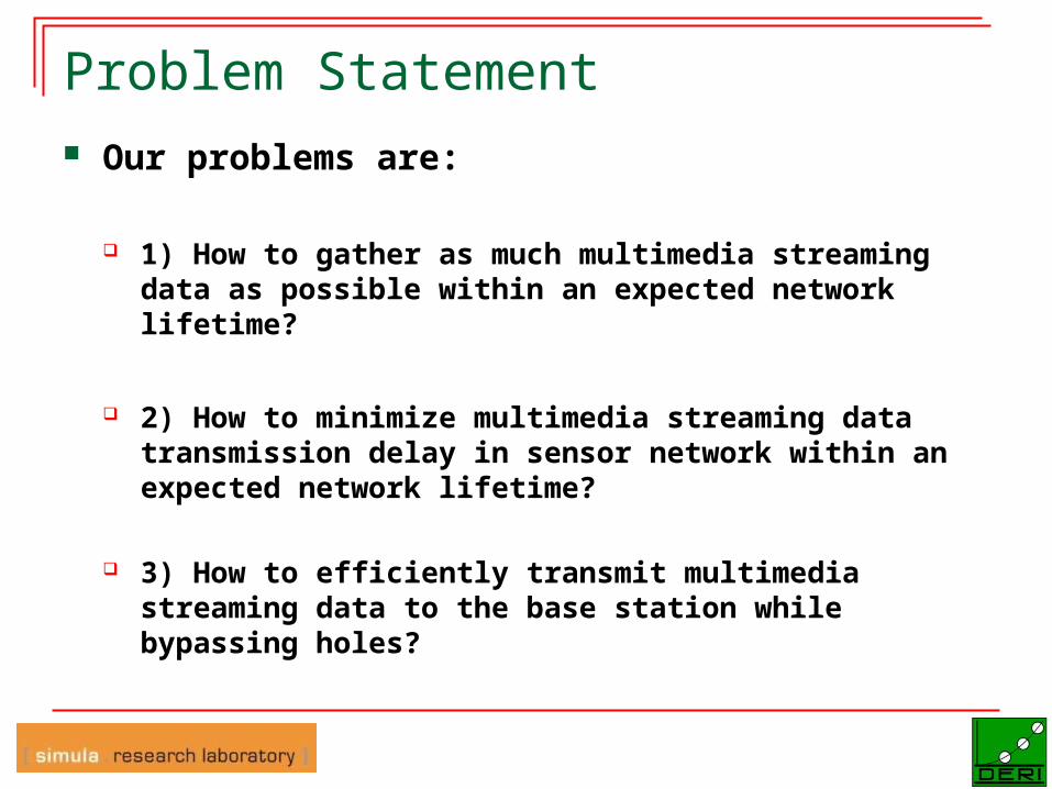
Problem Statement Our problems are:
1) How to gather as much multimedia streaming data as possible within an expected network lifetime?
2) How to minimize multimedia streaming data transmission delay in sensor network within an expected network lifetime?
3) How to efficiently transmit multimedia streaming data to the base station while bypassing holes?
Wireless Sensor NetworksDigital Enterprise Research
Institute
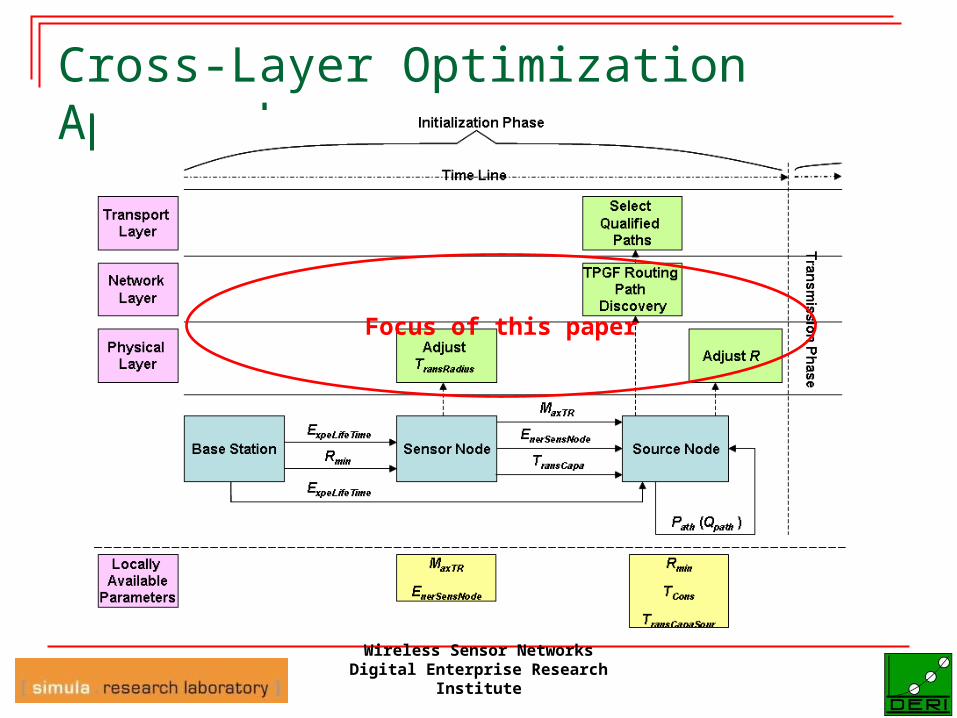
Cross-Layer Optimization Approach
Focus of this paper
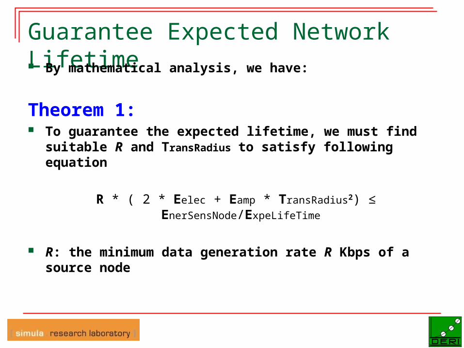
Guarantee Expected Network Lifetime By mathematical analysis, we have:
Theorem 1: To guarantee the expected lifetime, we must find
suitable R and TransRadius to satisfy following equation
R * ( 2 * Eelec + Eamp * TransRadius2) ≤ EnerSensNode/ExpeLifeTime
R: the minimum data generation rate R Kbps of a source node
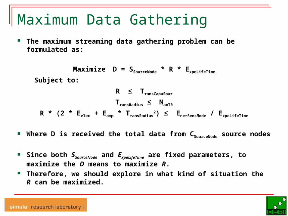
Maximum Data Gathering The maximum streaming data gathering problem can be
formulated as:
Maximize D = SSourceNode * R * ExpeLifeTime
Subject to:
R ≤ TransCapaSour
TransRadius ≤ MaxTR
R * (2 * Eelec + Eamp * TransRadius2) ≤ EnerSensNode / ExpeLifeTime
Where D is received the total data from CSourceNode source nodes
Since both SSourceNode and ExpeLifeTime are fixed parameters, to maximize the D means to maximize R.
Therefore, we should explore in what kind of situation the R can be maximized.
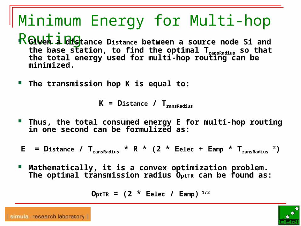
Minimum Energy for Multi-hop Routing Given a distance Distance between a source node Si and
the base station, to find the optimal TransRadius so that the total energy used for multi-hop routing can be minimized.
The transmission hop K is equal to:
K = Distance / TransRadius
Thus, the total consumed energy E for multi-hop routing in one second can be formulized as:
E = Distance / TransRadius * R * (2 * Eelec + Eamp * TransRadius 2)
Mathematically, it is a convex optimization problem. The optimal transmission radius OptTR can be found as:
OptTR = (2 * Eelec / Eamp) 1/2

Energy Consumption Rate The energy consumption rate ECR(MaxTR) of sensor
nodes when they are using MaxTR can be formulized as:
ECR(MaxTR) = R * (2 * Eelec + Eamp * MaxTR2)
The energy consumption rate ECR(OptTR) can be formulized as:
ECR(OptTR) = R * (2 * Eelec + Eamp * OptTR2)
The energy consumption rate of sensor nodes when using ExpTR to transmit stream data can be formulized as:
ECR(ExpTR) = R * (2 * Eelec + Eamp * ExpTR2)
Where ExpTR = ((EnerSensNode / (ExpeLifeTime * R) - 2 * Eelec) / Eamp) 1/2
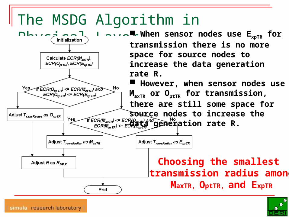
The MSDG Algorithm in Physical Layer
Choosing the smallest transmission radius among
MaxTR, OptTR, and ExpTR
When sensor nodes use ExpTR for transmission there is no more space for source nodes to increase the data generation rate R. However, when sensor nodes use MaxTR or OptTR for transmission, there are still some space for source nodes to increase the data generation rate R.
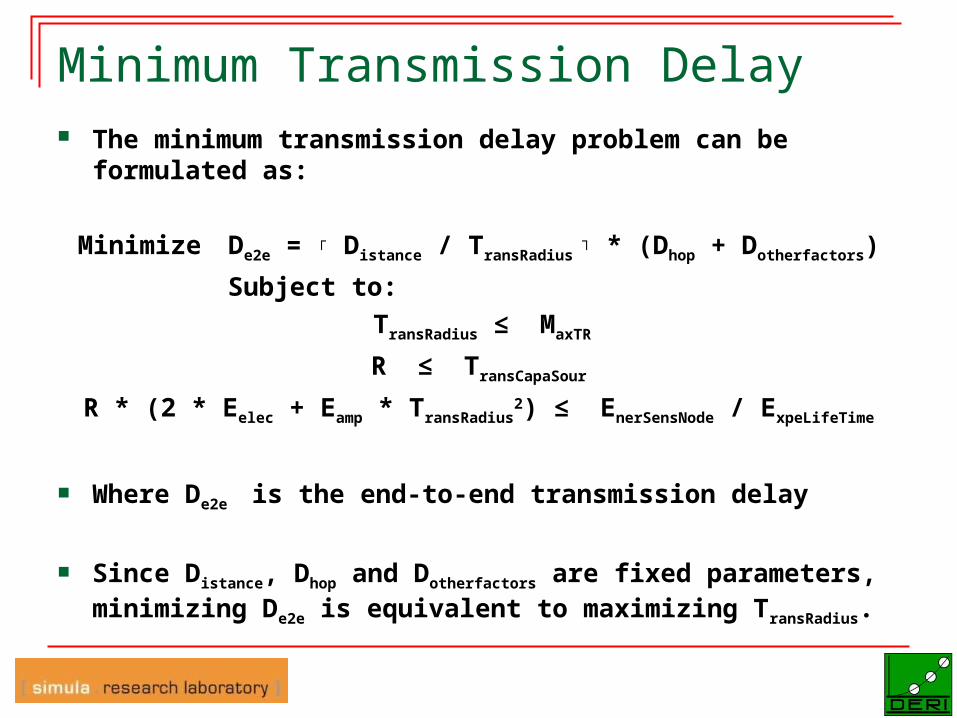
Minimum Transmission Delay The minimum transmission delay problem can be
formulated as:
Minimize De2e = ┌ Distance / TransRadius ┐ * (Dhop + Dotherfactors)
Subject to: TransRadius ≤ MaxTR
R ≤ TransCapaSour
R * (2 * Eelec + Eamp * TransRadius2) ≤ EnerSensNode / ExpeLifeTime
Where De2e is the end-to-end transmission delay
Since Distance, Dhop and Dotherfactors are fixed parameters, minimizing De2e is equivalent to maximizing TransRadius.
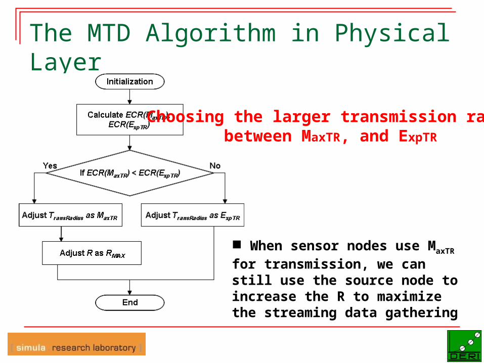
The MTD Algorithm in Physical Layer
Choosing the larger transmission radiusbetween MaxTR, and ExpTR
When sensor nodes use MaxTR for transmission, we can still use the source node to increase the R to maximize the streaming data gathering
Routing Algorithm in Network Layer Design a new routing protocol to facilitate the
multimedia streaming data transmission in wireless multimedia sensor networks.
Hole-bypassing, the designed routing algorithm should be able to bypass holes
Guarantee path exploration result, the designed routing algorithm should be able to find the routing paths if they exist
Routing path optimization, the designed routing algorithm should be able to optimize each routing path with less number of transmission hops
Node-disjoint multi-path transmission, the designed routing algorithm should be able to be executed repeatedly to find multiple node-disjoint routing paths
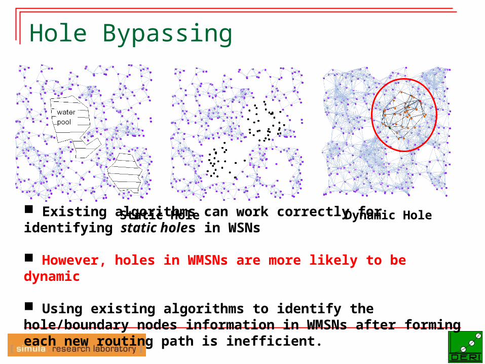
Hole Bypassing
Existing algorithms can work correctly for identifying static holes in WSNs
However, holes in WMSNs are more likely to be dynamic
Using existing algorithms to identify the hole/boundary nodes information in WMSNs after forming each new routing path is inefficient.
Static Hole Dynamic Hole
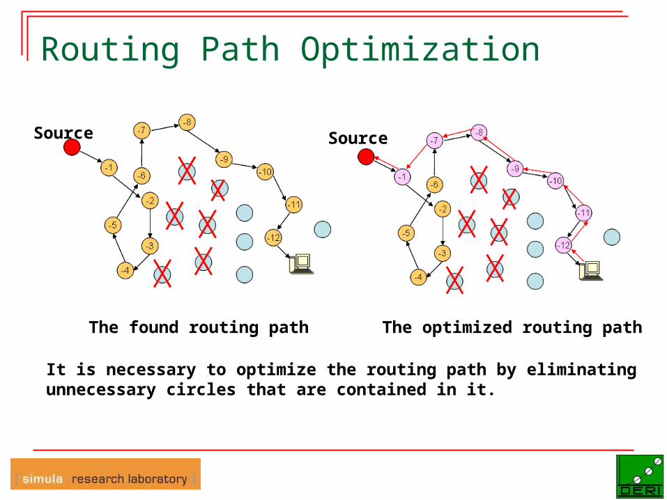
Routing Path Optimization
The found routing path The optimized routing path
It is necessary to optimize the routing path by eliminating unnecessary circles that are contained in it.
Source Source
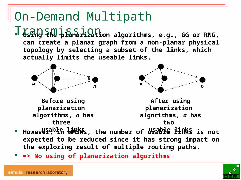
On-Demand Multipath Transmission Using the planarization algorithms, e.g., GG or RNG,
can create a planar graph from a non-planar physical topology by selecting a subset of the links, which actually limits the useable links.
However, in WMSNs, the number of usable links is not expected to be reduced since it has strong impact on the exploring result of multiple routing paths.
=> No using of planarization algorithms
Before using planarization
algorithms, a has three
usable links
After using planarization
algorithms, a has two
usable links
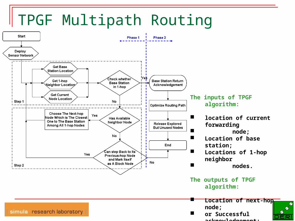
TPGF Multipath Routing Algorithm
The inputs of TPGF algorithm:
location of current forwarding node; Location of base station; Locations of 1-hop neighbor nodes. The outputs of TPGF algorithm:
Location of next-hop node; or Successful
acknowledgement; or Unsuccessful
acknowledgement.
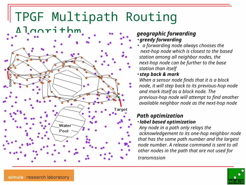
TPGF Multipath Routing Algorithm geographic forwarding
•greedy forwarding• a forwarding node always chooses the next-hop node which is closest to the based station among all neighbor nodes, the next-hop node can be further to the base station than itself •step back & mark When a sensor node finds that it is a block node, it will step back to its previous-hop node and mark itself as a block node. The previous-hop node will attempt to find another available neighbor node as the next-hop node
Path optimization•label based optimization Any node in a path only relays the acknowledgement to its one-hop neighbor node that has the same path number and the largest node number. A release command is sent to all other nodes in the path that are not used for
transmission
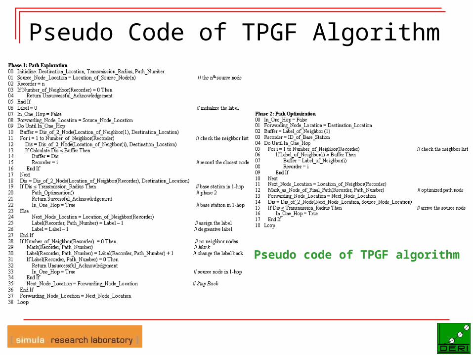
Pseudo Code of TPGF Algorithm
Pseudo code of TPGF algorithm
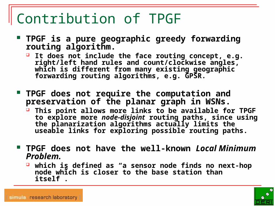
Contribution of TPGF TPGF is a pure geographic greedy forwarding
routing algorithm. It does not include the face routing concept, e.g.
right/left hand rules and count/clockwise angles, which is different from many existing geographic forwarding routing algorithms, e.g. GPSR.
TPGF does not require the computation and preservation of the planar graph in WSNs. This point allows more links to be available for TPGF
to explore more node-disjoint routing paths, since using the planarization algorithms actually limits the useable links for exploring possible routing paths.
TPGF does not have the well-known Local
Minimum Problem. which is defined as “a sensor node finds no next-hop
node which is closer to the base station than itself”.
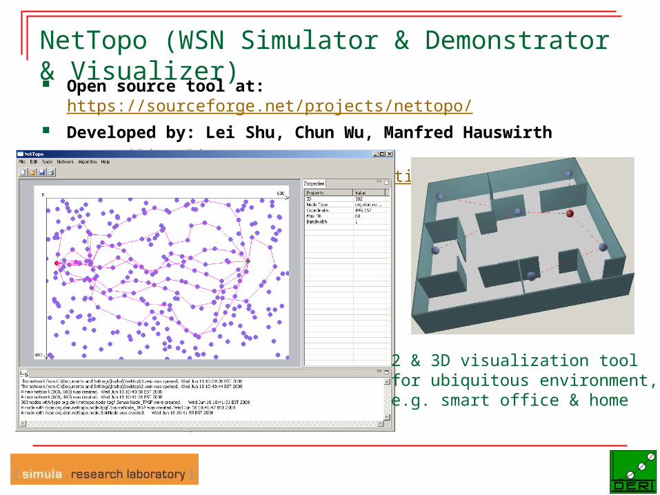
NetTopo (WSN Simulator & Demonstrator & Visualizer) Open source tool at: https://sourceforge.net/projects/nettopo/ Developed by: Lei Shu, Chun Wu, Manfred Hauswirth Our mailing list: http://lists.deri.org/mailman/listinfo/nettopo
2 & 3D visualization tool for ubiquitous environment, e.g. smart office & home
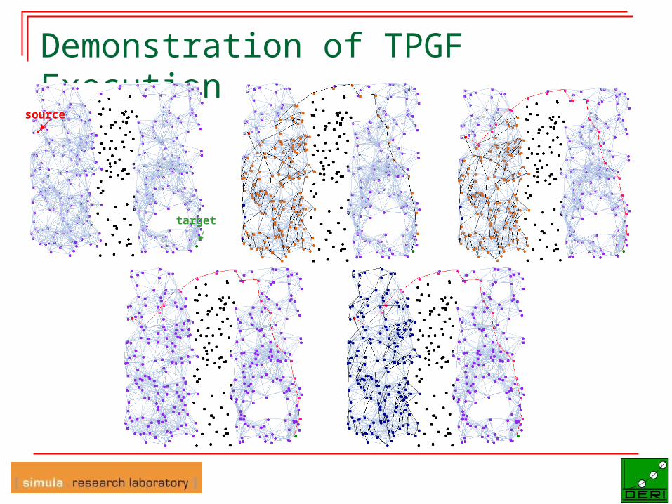
Demonstration of TPGF Execution
source
target
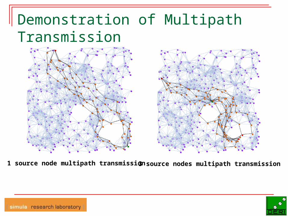
Demonstration of Multipath Transmission
1 source node multipath transmission 3 source nodes multipath transmission
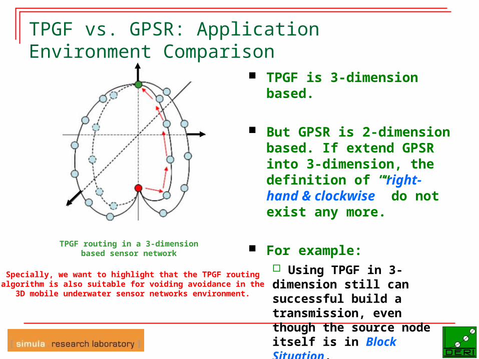
TPGF vs. GPSR: Application Environment Comparison
TPGF is 3-dimension based.
But GPSR is 2-dimension based. If extend GPSR into 3-dimension, the definition of “right-hand & clockwise” do not exist any more.
For example: Using TPGF in 3-dimension still can successful build a transmission, even though the source node itself is in Block Situation.
TPGF routing in a 3-dimension based sensor network
Specially, we want to highlight that the TPGF routing algorithm is also suitable for voiding avoidance in the 3D mobile underwater sensor networks environment.
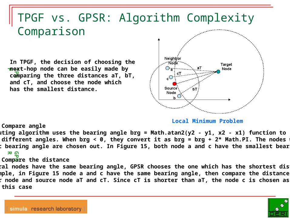
TPGF vs. GPSR: Algorithm Complexity Comparison
Local Minimum Problem Step 1: Compare angleGPSR routing algorithm uses the bearing angle brg = Math.atan2(y2 - y1, x2 - x1) function to compare different angles. When brg < 0, they convert it as brg = brg + 2* Math.PI. The nodes with the smallest bearing angle are chosen out. In Figure 15, both node a and c have the smallest bearing angle.
Step 2: Compare the distanceIf several nodes have the same bearing angle, GPSR chooses the one which has the shortest distance. For example, in Figure 15 node a and c have the same bearing angle, then compare the distance between neighbor node and source node aT and cT. Since cT is shorter than aT, the node c is chosen as the next-hop node in this case
GP
SR
TP
GF In TPGF, the decision of choosing the
next-hop node can be easily made by comparing the three distances aT, bT, and cT, and choose the node which has the smallest distance.
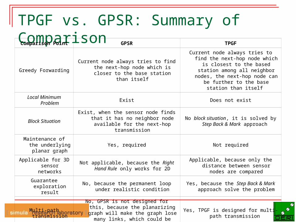
TPGF vs. GPSR: Summary of ComparisonComparison Point GPSR TPGF
Greedy ForwardingCurrent node always tries to find the next-hop
node which is closer to the base station than itself
Current node always tries to find the next-hop node which is closest to the based station among all neighbor nodes, the next-hop node can be further to the base station
than itself
Local Minimum Problem Exist Does not exist
Block SituationExist, when the sensor node finds that it has no
neighbor node available for the next-hop transmission
No block situation, it is solved by Step Back & Mark approach
Maintenance of the underlying planar
graphYes, required Not required
Applicable for 3D sensor networks
Not applicable, because the Right Hand Rule only works for 2D
Applicable, because only the distance between sensor nodes are compared
Guarantee exploration result
No, because the permanent loop under realistic condition
Yes, because the Step Back & Mark approach solve the problem
Multi-path transmission
No, GPSR is not designed for this, because the planarizing graph will make the graph lose
many links, which could be used in the multiple paths
Yes, TPGF is designed for multi-path transmission
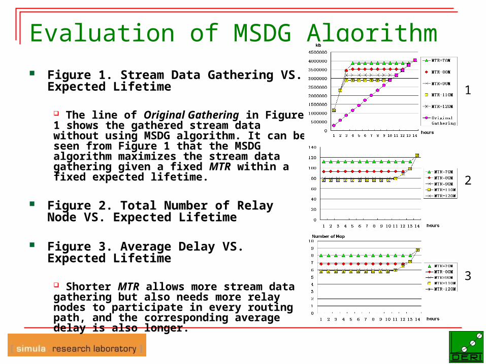
Evaluation of MSDG Algorithm Figure 1. Stream Data Gathering VS.
Expected Lifetime
The line of Original Gathering in Figure 1 shows the gathered stream data without using MSDG algorithm. It can be seen from Figure 1 that the MSDG algorithm maximizes the stream data gathering given a fixed MTR within a fixed expected lifetime.
Figure 2. Total Number of Relay Node VS. Expected Lifetime
Figure 3. Average Delay VS. Expected Lifetime
Shorter MTR allows more stream data gathering but also needs more relay nodes to participate in every routing path, and the corresponding average delay is also longer.
1
2
3
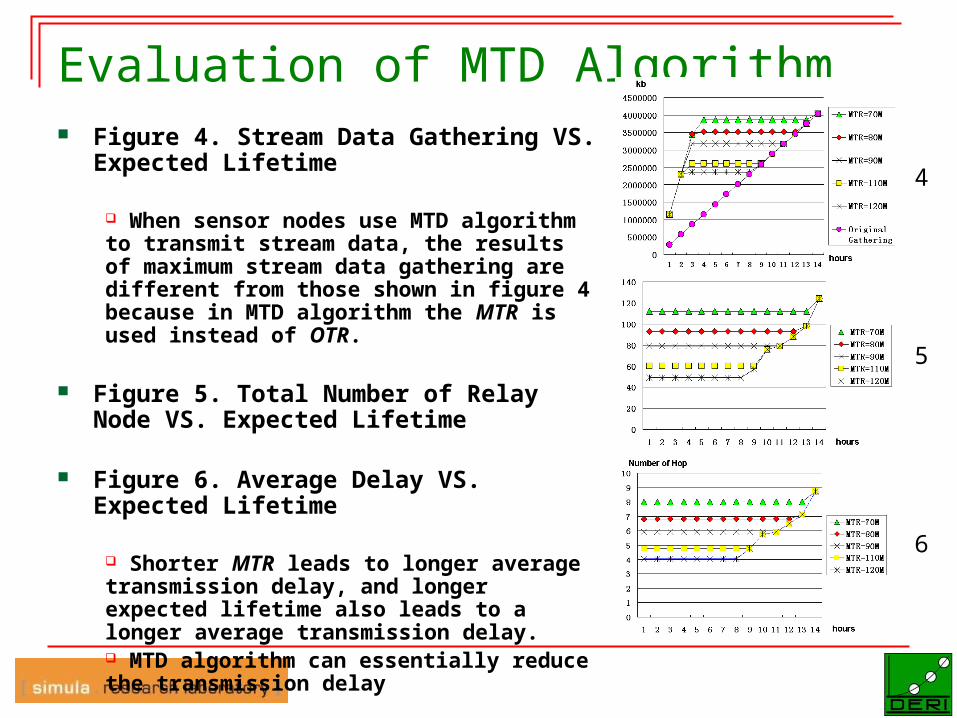
Evaluation of MTD Algorithm Figure 4. Stream Data Gathering VS.
Expected Lifetime
When sensor nodes use MTD algorithm to transmit stream data, the results of maximum stream data gathering are different from those shown in figure 4 because in MTD algorithm the MTR is used instead of OTR.
Figure 5. Total Number of Relay Node VS. Expected Lifetime
Figure 6. Average Delay VS. Expected Lifetime
Shorter MTR leads to longer average transmission delay, and longer expected lifetime also leads to a longer average transmission delay. MTD algorithm can essentially reduce the transmission delay
4
5
6

GPSR vs. TPGF: Execution Comparison
(a) Running GPSR in the GG virtual WSN with 4 routing paths when TR is set as 60 meters
(b)Running GPSR in the RNG virtual WSN with 4 routing paths when TR is set as 60 meters
(c)Running TPGF in the virtual WSN with 4 routing paths when TR is set as 60 meters
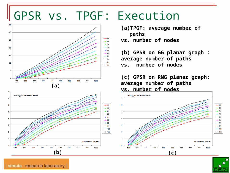
GPSR vs. TPGF: Execution Comparison (a)TPGF: average number of
paths vs. number of nodes
(b) GPSR on GG planar graph : average number of paths vs. number of nodes
(c) GPSR on RNG planar graph: average number of paths vs. number of nodes
(a)
(b) (c)
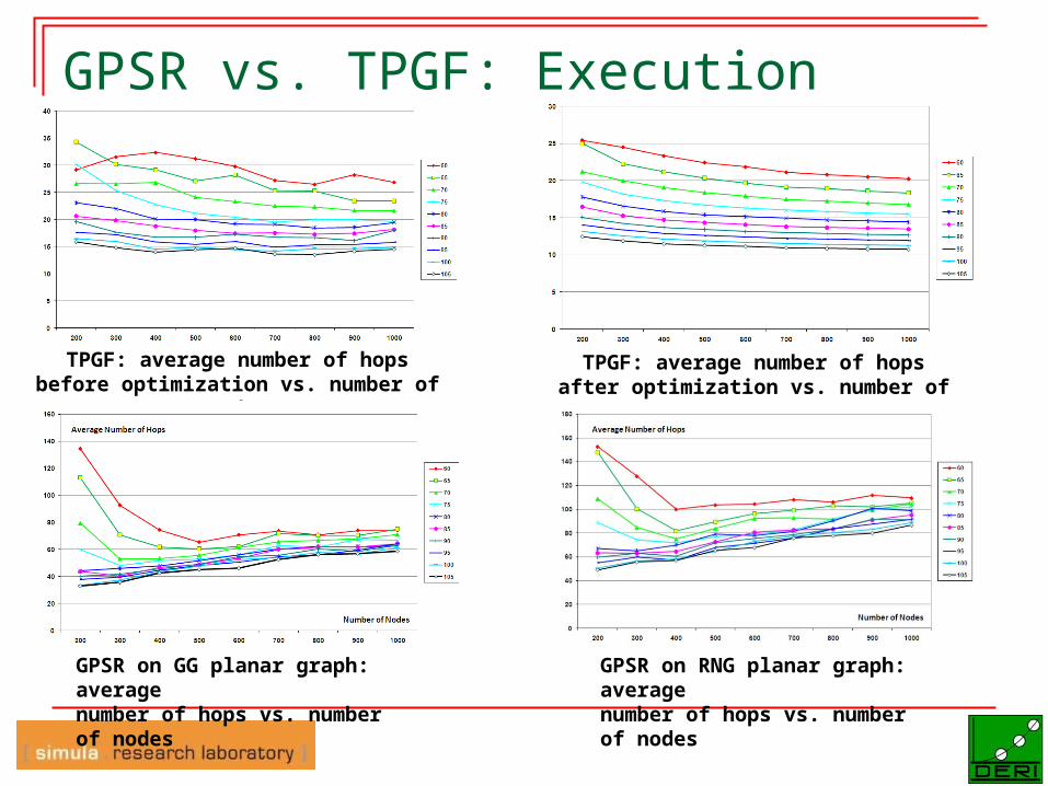
GPSR vs. TPGF: Execution Comparison
TPGF: average number of hops before optimization vs. number of
nodes
TPGF: average number of hops after optimization vs. number of
nodes
GPSR on GG planar graph: average number of hops vs. number of nodes
GPSR on RNG planar graph: average number of hops vs. number of nodes
Conclusion Studied two important research problems:
1) maximizing stream data gathering in wireless sensor networks within expected lifetime;
2) minimizing transmission delay for stream data gathering in wireless sensor networks within expected lifetime.
Either of these two algorithms should be run in the initializing phase in every node of whole sensor network for choosing the appropriate transmission radius.
When generate rate R of source nodes is larger than the maximum transmission capacity of sensor nodes, we find that using node-disjoint multi-path transmission can solve the problem.
Our algorithms can be used in various applications when
video sensor nodes, audio sensor nodes, or any type of sensor nodes are deployed in sensor networks for gathering stream data continuously during a short amount of time.
Reference L. Shu, Y. Zhang, G. Min, Y. Wang, M. Hauswirth, "Cross-Layer
Optimization on Data Gathering in Wireless Multimedia Sensor Networks within Expected Network Lifetime", submitted to Springer Journal of Universal Computer Science (JUCS), 2008.
L. Shu, Y. Zhang, Z. Zhou, M. Hauswirth, Z. Yu, G. Hynes, "Transmitting and Gathering Streaming Data in Wireless Multimedia Sensor Networks within Expected Network Lifetime", accepted in ACM/Springer Journal Mobile Networks and Applications (MONET), 2008.
L. Shu, Z. Zhou, M. Hauswirth, D. Phuoc, P. Yu, L. Zhang, "Transmitting Streaming Data in Wireless Multimedia Sensor Networks with Holes", the Sixth International Conference on Mobile and Ubiquitous Multimedia (MUM 2007 acceptance rate: 21%), December 12-14, 2007. Oulu, Finland.
L. Shu, Z. Zhou, A. Aguilar, M. Hauswirth, "Stream Data Gathering in Wireless (multimedia) Sensor Networks within Expected Lifetime", the third ACM International Mobile Multimedia Communications Conference, (MobiMedia 2007), August 27-29, 2007 Nafpaktos Greece.
Thanks