Transmission Lines and Power Flow Analysis - UMN … Lines and Power Flow Analysis Dr. Greg Mowry...

Transmission Lines and

Power Flow Analysis

Dr. Greg Mowry

Annie Sebastian

Marian Mohamed

School of Engineering (SOE)

University of St Thomas (UST)

1

2

The UST Mission

Inspired by Catholic intellectual tradition, the

University of St. Thomas educates students

to be morally responsible leaders who think

critically, act wisely, and work skillfully to

advance the common good. http://www.stthomas.edu/mission/

Since civilization depends on power, power is for the

‘common good’!!

School of Engineering

http://www.stthomas.edu/mission/

Outline

I. Background material

II. Transmission Lines (TLs)

III. Power Flow Analysis (PFA)


3

I. Background Material


4

Networks & Power Systems

In a network (power system) there are 6 basic

electrical quantities of interest:

1. Current 𝑖 𝑡 = 𝑑𝑞/𝑑𝑡

2. Voltage 𝑣 𝑡 = 𝑑𝜑/𝑑𝑡 (FL)

3. Power 𝑝 𝑡 = 𝑣 𝑡 𝑖 𝑡 =𝑑𝑤

𝑑𝑡=

𝑑𝐸

𝑑𝑡


5


6 basic electrical quantities continued:

4. Energy (work) w t = −∞

𝑡𝑝 𝜏 𝑑𝜏 = −∞

𝑡𝑣 𝜏 𝑖 𝜏 𝑑𝜏

5. Charge (q or Q) 𝑞 𝑡 = −∞

𝑡𝑖 𝜏 𝑑𝜏

6. Flux 𝜑 𝑡 = −∞

𝑡𝑣 𝜏 𝑑𝜏


6


A few comments:

Voltage (potential) has potential-energy characteristics

and therefore needs a reference to be meaningful; e.g.

ground 0 volts

I will assume that pretty much everything we discuss

& analyze today is linear until we get to PFA


7


Linear Time Invariant (LTI) systems:

Linearity:

If 𝑦1 = 𝑓 𝑥1 & 𝑦2 = 𝑓(𝑥2)

Then 𝛼 𝑦1 + 𝛽 𝑦2 = 𝑓(𝛼 𝑥1 + 𝛽 𝑥2)


8


Implications of LTI systems:

Scalability: if 𝑦 = 𝑓(𝑥), then 𝛼𝑦 = 𝑓(𝛼𝑥)

Superposition & scalability of inputs holds

Frequency invariance: 𝜔𝑖𝑛𝑝𝑢𝑡 = 𝜔𝑜𝑢𝑡𝑝𝑢𝑡


9


ACSS and LTI systems:

Suppose: 𝑣𝑖𝑛 𝑡 = 𝑉𝑖𝑛 cos 𝜔𝑡 + 𝜃

Since input = output, the only thing a linear system can

do to an input is:

Change the input amplitude: Vin Vout

Change the input phase: in out


10



These LTI characteristics along with Euler’s theorem

𝑒𝑗𝜔𝑡 = cos 𝜔𝑡 + 𝑗 sin 𝜔𝑡 ,

allow 𝑣𝑖𝑛 𝑡 = 𝑉𝑖 cos 𝜔𝑡 + 𝜃 to be represented as

𝑣𝑖𝑛 𝑡 = 𝑉𝑖 cos 𝜔𝑡 + 𝜃 𝑉𝑖𝑒𝑗𝜃 = 𝑉𝑖 ∠𝜃


11


In honor of Star Trek,

𝑉𝑖𝑒𝑗𝜃 = 𝑉𝑖 ∠𝜃

is called a ‘Phasor’


12


13𝑉𝑖𝑒𝑗𝜃 = 𝑉𝑖 ∠𝜃



Since time does not explicitly appear in a phasor, an

LTI system in ACSS can be treated like a DC system

on steroids with j

ACSS also requires impedances; i.e. AC resistance


14


Comments:

Little, if anything, in ACSS analysis is gained by

thinking of j = −1 (that is algebra talk)

Rather, since Euler Theorem looks similar to a 2D

vector

𝑒𝑗𝜔𝑡 = cos 𝜔𝑡 + 𝑗 sin 𝜔𝑡

𝑢 = 𝑎 𝑥 + 𝑏 𝑦


15


16

𝑒𝑗90° = cos 90° + 𝑗 sin 90° = 𝑗

Hence in ACSS analysis,

think of j as a 90 rotation

Operators


17

)(tv VV

dt

dvVj

vdtj

V

Ohm’s Approximation (Law)


Summary of voltage-current relationship

Element Time domain Frequency domain

R

L

C

Riv RIV

dt

diLv LIjV

dt

dvCi

Cj

IV

18

Impedance & Admittance


18

RY

1

LjY

1

CjY

Impedances and admittances of passive elements

Element Impedance Admittance

R

L

C

RZ

LjZ

CjZ

1

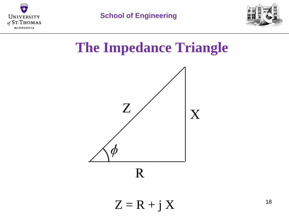
The Impedance Triangle


18Z = R + j X

The Power Triangle (ind. reactance)


18S = P + j Q

Triangles

Comments:

Power Triangle = Impedance Triangle

The cos() defines the Power Factor (pf)


22

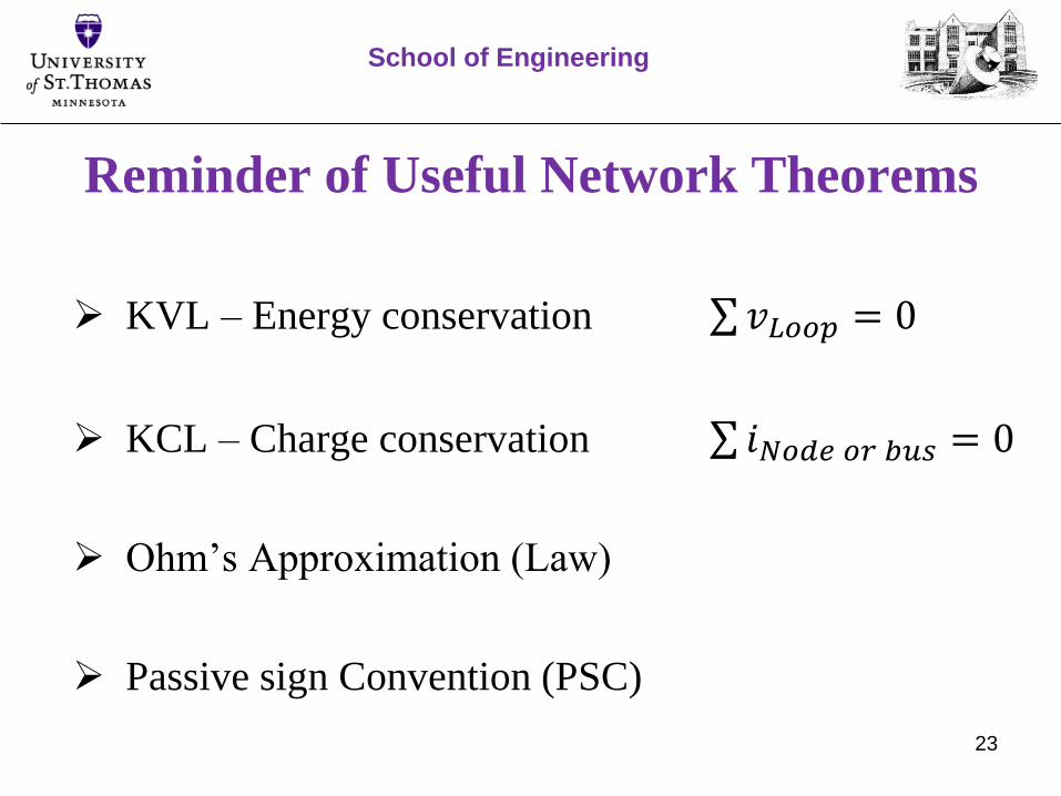
Reminder of Useful Network Theorems

KVL – Energy conservation 𝑣𝐿𝑜𝑜𝑝 = 0

KCL – Charge conservation 𝑖𝑁𝑜𝑑𝑒 𝑜𝑟 𝑏𝑢𝑠 = 0

Ohm’s Approximation (Law)

Passive sign Convention (PSC)


23

Passive Sign Convection – Power System


24

PSC


25

Source Load or Circuit Element

PSource = vi PLoad = vi

PSource = PLoad

Reminder of Useful Network Theorems

Pointing Theorem 𝑆 = 𝑉 𝐼∗

Thevenin Equivalent – Any linear circuit may be

represented by a voltage source and series Thevenin

impedance

Norton Equivalent – Any linear circuit my be

represented by a current source and a shunt Thevenin

impedance

𝑉𝑇𝐻 = 𝐼𝑁 𝑍𝑇𝐻


26

Transmission Lines and

Power Flow Analysis

Dr. Greg Mowry

Annie Sebastian

Marian Mohamed

School of Engineering (SOE)

University of St Thomas (UST)

1

II. Transmission Lines


2

Outline

General Aspects of TLs

TL Parameters: R, L, C, G

2-Port Analysis (a brief interlude)

Maxwell’s Equations & the Telegraph equations

Solutions to the TL wave equations


3


4


5

Transmission Lines (TLs)

A TL is a major component of an electrical

power system.

The function of a TL is to transport power

from sources to loads with minimal loss.


6

Transmission Lines

In an AC power system, a TL will operate

at some frequency f; e.g. 60 Hz.

Consequently, 𝜆 = 𝑐/𝑓

The characteristics of a TL manifest

themselves when 𝝀 ~ 𝑳 of the system.


7

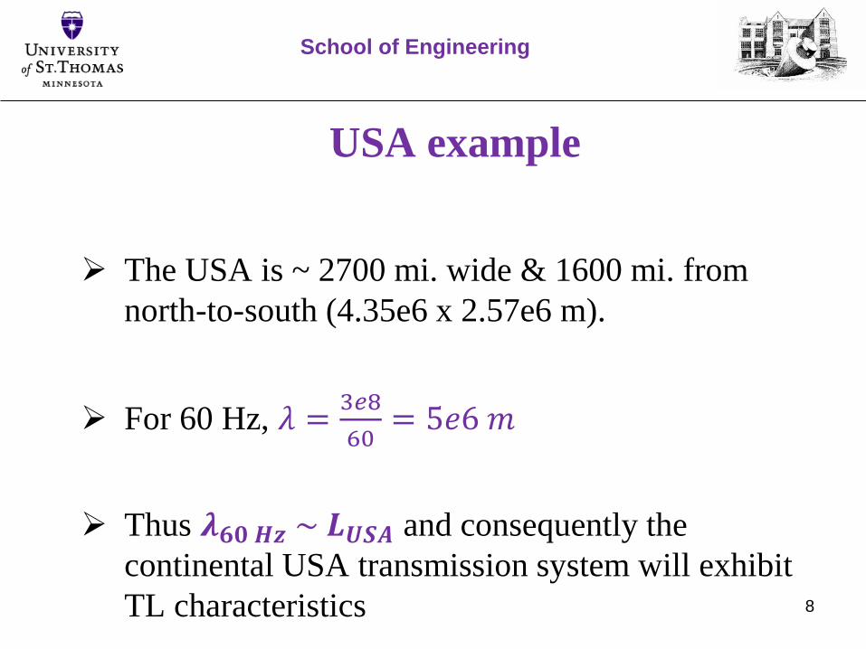
USA example

The USA is ~ 2700 mi. wide & 1600 mi. from

north-to-south (4.35e6 x 2.57e6 m).

For 60 Hz, 𝜆 =3𝑒8

60= 5𝑒6 𝑚

Thus 𝝀𝟔𝟎 𝑯𝒛 ~ 𝑳𝑼𝑺𝑨 and consequently the

continental USA transmission system will exhibit

TL characteristics


8

Overhead TL Components


9

Overhead ACSR TL Cables


10

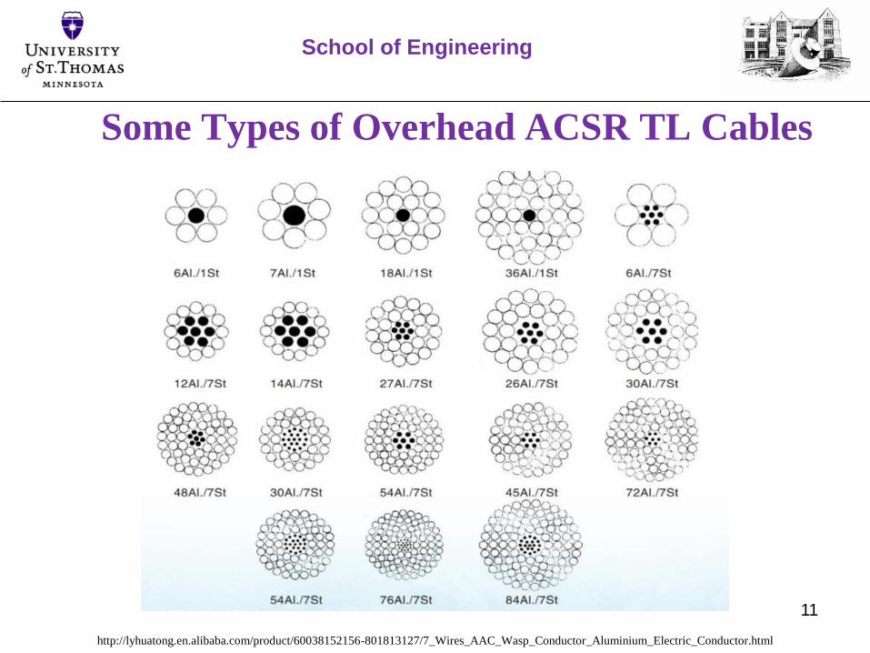
Some Types of Overhead ACSR TL Cables


11

http://lyhuatong.en.alibaba.com/product/60038152156-801813127/7_Wires_AAC_Wasp_Conductor_Aluminium_Electric_Conductor.html

TL Parameters


12

13

Model of an Infinitesimal TL Section


General TL Parameters

a. Series Resistance – accounts for Ohmic (I2R losses)

b. Series Impedance – accounts for series voltage drops

Resistive

Inductive reactance

c. Shunt Capacitance – accounts for Line-Charging Currents

d. Shunt Conductance – accounts for V2G losses due to leakage

currents between conductors or between conductors and

ground.


14

Power TL Parameters

Series Resistance: related to the physical structure of

the TL conductor over some temperature range.

Series Inductance & Shunt Capacitance: produced

by magnetic and electric fields around the conductor

and affected by their geometrical arrangement.

Shunt Conductance: typically very small so

neglected.


15

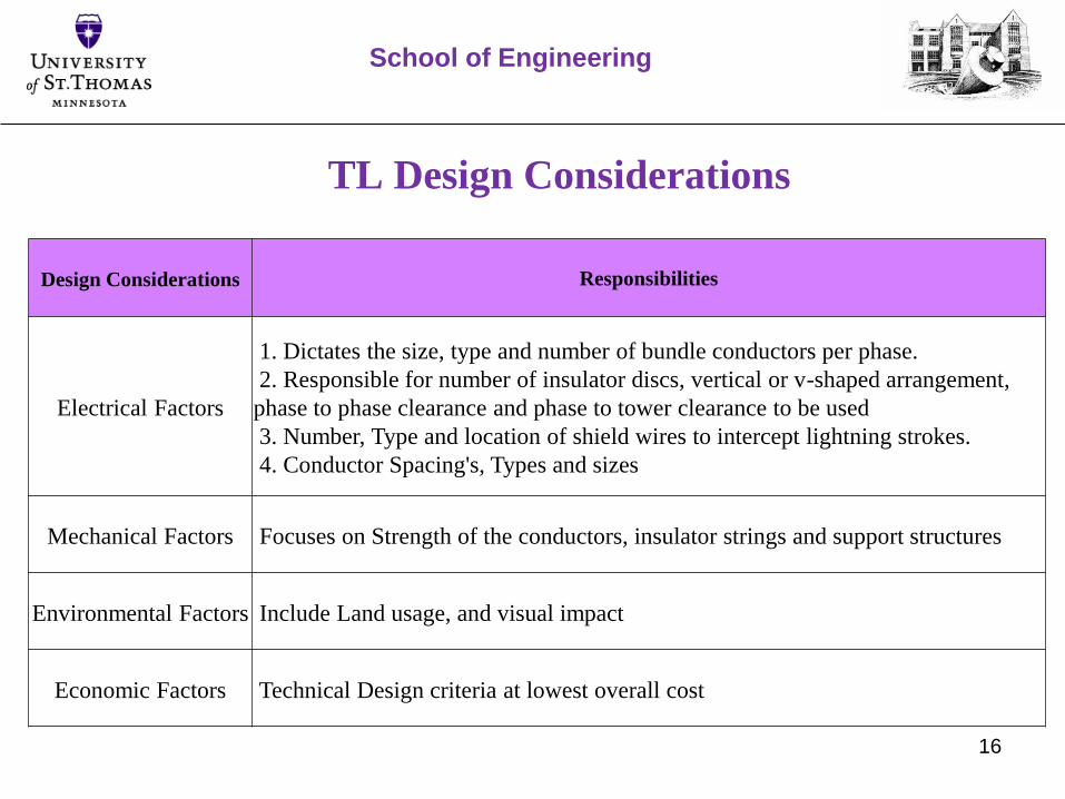
TL Design Considerations


Design Considerations Responsibilities

Electrical Factors

1. Dictates the size, type and number of bundle conductors per phase.

2. Responsible for number of insulator discs, vertical or v-shaped arrangement,

phase to phase clearance and phase to tower clearance to be used

3. Number, Type and location of shield wires to intercept lightning strokes.

4. Conductor Spacing's, Types and sizes

Mechanical Factors Focuses on Strength of the conductors, insulator strings and support structures

Environmental Factors Include Land usage, and visual impact

Economic Factors Technical Design criteria at lowest overall cost

16

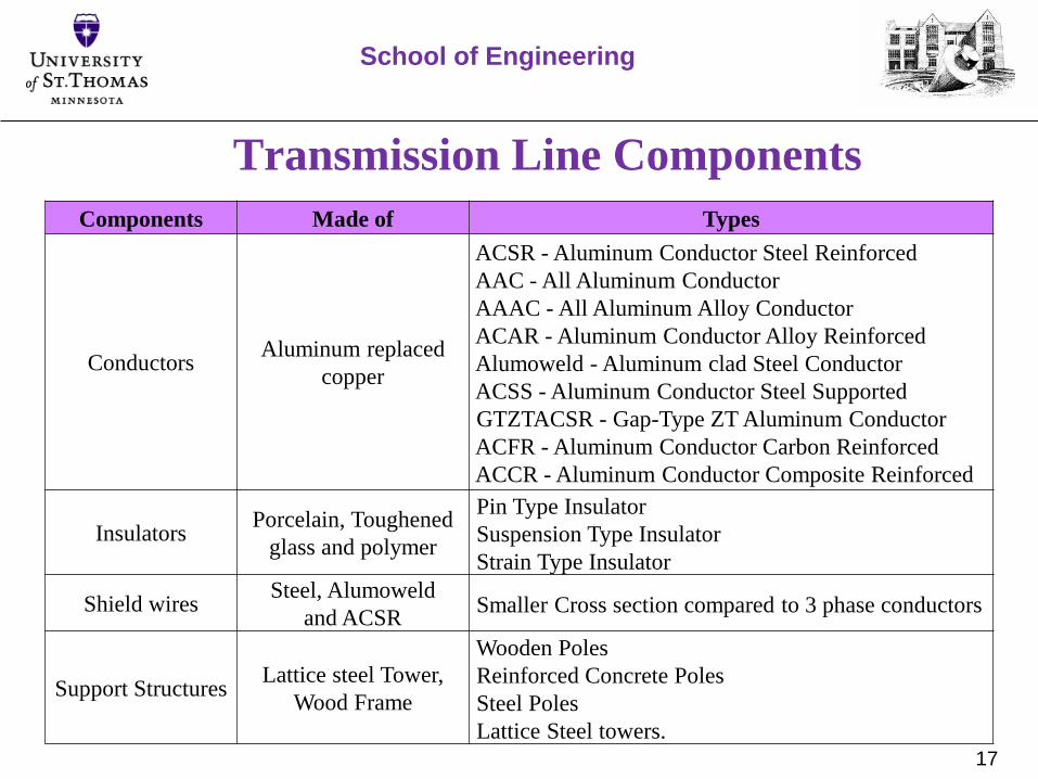
Transmission Line Components


Components Made of Types

ConductorsAluminum replaced

copper

ACSR - Aluminum Conductor Steel Reinforced

AAC - All Aluminum Conductor

AAAC - All Aluminum Alloy Conductor

ACAR - Aluminum Conductor Alloy Reinforced

Alumoweld - Aluminum clad Steel Conductor

ACSS - Aluminum Conductor Steel Supported

GTZTACSR - Gap-Type ZT Aluminum Conductor

ACFR - Aluminum Conductor Carbon Reinforced

ACCR - Aluminum Conductor Composite Reinforced

Insulators Porcelain, Toughened

glass and polymer

Pin Type Insulator

Suspension Type Insulator

Strain Type Insulator

Shield wiresSteel, Alumoweld

and ACSRSmaller Cross section compared to 3 phase conductors

Support StructuresLattice steel Tower,

Wood Frame

Wooden Poles

Reinforced Concrete Poles

Steel Poles

Lattice Steel towers.

17

ACSR Conductor Characteristic


NameOverall Dia

(mm)

DC Resistance

(ohms/km)

Current Capacity

(Amp) 75 C

Mole 4.5 2.78 70

Squirrel 6.33 1.394 107

Weasel 7.77 0.9291 138

Rabbit 10.05 0.5524 190

Racoon 12.27 0.3712 244

Dog 14.15 0.2792 291

Wolf 18.13 0.1871 405

Lynx 19.53 0.161 445

Panther 21 0.139 487

Zebra 28.62 0.06869 737

Dear 29.89 0.06854 756

Moose 31.77 0.05596 836

Bersimis 35.04 0.04242 998 18

TL Parameters - Resistance


19

TL conductor resistance depends on factors such

as:

Conductor geometry

The frequency of the AC current

Conductor proximity to other current-carrying conductors

Temperature


20

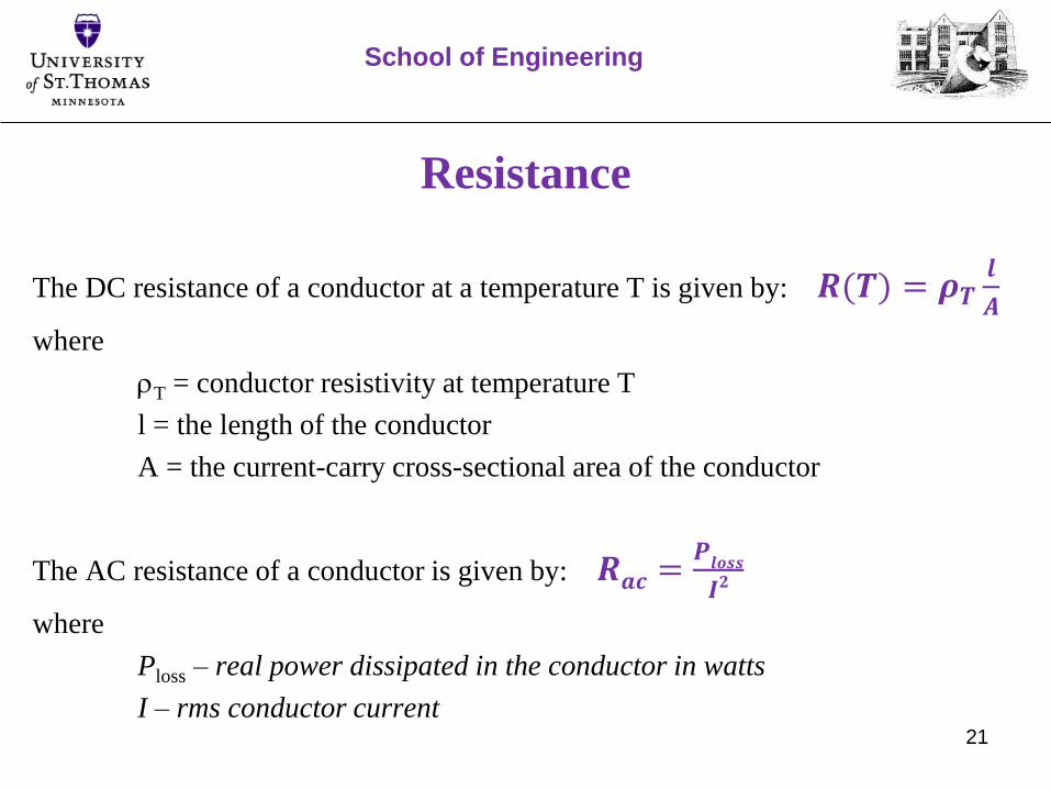
Resistance

The DC resistance of a conductor at a temperature T is given by: 𝑹(𝑻) = 𝝆𝑻𝒍

𝑨

where

T = conductor resistivity at temperature T

l = the length of the conductor

A = the current-carry cross-sectional area of the conductor

The AC resistance of a conductor is given by: 𝑹𝒂𝒄 =𝑷𝒍𝒐𝒔𝒔

𝑰𝟐

where

Ploss – real power dissipated in the conductor in watts

I – rms conductor current


21

TL Conductor Resistance depends on:

Spiraling:

The purpose of introducing a steel core inside the stranded

aluminum conductors is to obtain a high strength-to-weight ratio. A

stranded conductor offers more flexibility and easier to

manufacture than a solid large conductor. However, the total

resistance is increased because the outside strands are larger than

the inside strands on account of the spiraling.


22

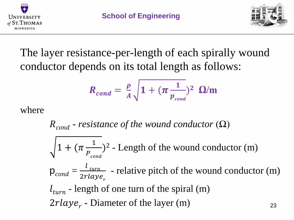
The layer resistance-per-length of each spirally wound

conductor depends on its total length as follows:

𝑹𝒄𝒐𝒏𝒅 =𝝆

𝑨𝟏 + (𝝅

𝟏

𝒑𝒄𝒐𝒏𝒅

)𝟐 Ω/m

where

𝑅𝑐𝑜𝑛𝑑 - resistance of the wound conductor (Ω)

1 + (𝜋1

𝑃𝑐𝑜𝑛𝑑

)2 - Length of the wound conductor (m)

p𝑐𝑜𝑛𝑑 = 𝑙𝑡𝑢𝑟𝑛

2𝑟𝑙𝑎𝑦𝑒𝑟

- relative pitch of the wound conductor (m)

𝑙𝑡𝑢𝑟𝑛 - length of one turn of the spiral (m)

2𝑟𝑙𝑎𝑦𝑒𝑟 - Diameter of the layer (m)


23

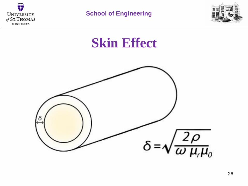
Frequency:

When voltages and currents change in time, current flow (i.e. current

density) is not uniform across the diameter of a conductor.

Thus the ‘effective’ current-carrying cross-section of a conductor with

AC is less than that for DC.

This phenomenon is known as skin effect.

As frequency increases, the current density decreases from that at the

surface of the conductor to that at the center of the conductor.


24

Frequency cont.

The spatial distribution of the current density in a particular conductor is

additionally altered (similar to the skin effect) due to currents in adjacent

current-carrying conductors.

This is called the ‘Proximity Effect’ and is smaller than the skin-effect.

Using the DC resistance as a starting point, the effect of AC on the

overall cable resistance may be accounted for by a correction factor k.

k is determined by E&M analysis. For 60 Hz, k is estimated around 1.02

𝑹𝑨𝑪 = 𝒌 𝑹𝑫𝑪


25

26

Skin Effect


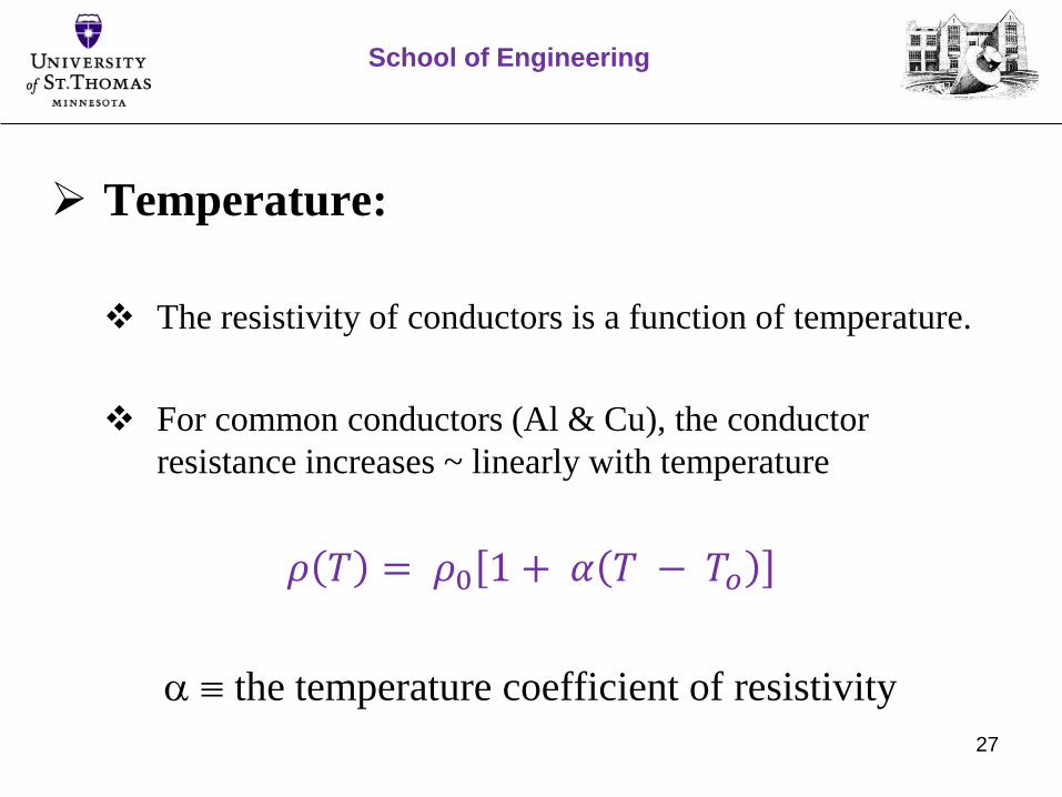
Temperature:

The resistivity of conductors is a function of temperature.

For common conductors (Al & Cu), the conductor

resistance increases ~ linearly with temperature

𝜌 𝑇 = 𝜌0 1 + 𝛼 𝑇 − 𝑇𝑜

the temperature coefficient of resistivity


27

TL Parameters - Conductance


28

Conductance

Conductance is associated with power losses between the

conductors or between the conductors and ground.

Such power losses occur through leakage currents on insulators

and via a corona

Leakage currents are affected by:

Contaminants such dirt and accumulated salt accumulated on insulators.

Meteorological factors such as moisture


29

Conductance

Corona loss occurs when the electric field at the surface of a

conductor causes the air to ionize and thereby conduct.

Corona loss depends on:

Conductor surface irregularities

Meteorological conditions such as humidity, fog, and rain

Losses due to leakage currents and corona loss are often small

compared to direct I2R losses on TLs and are typically neglected

in power flow studies.


30

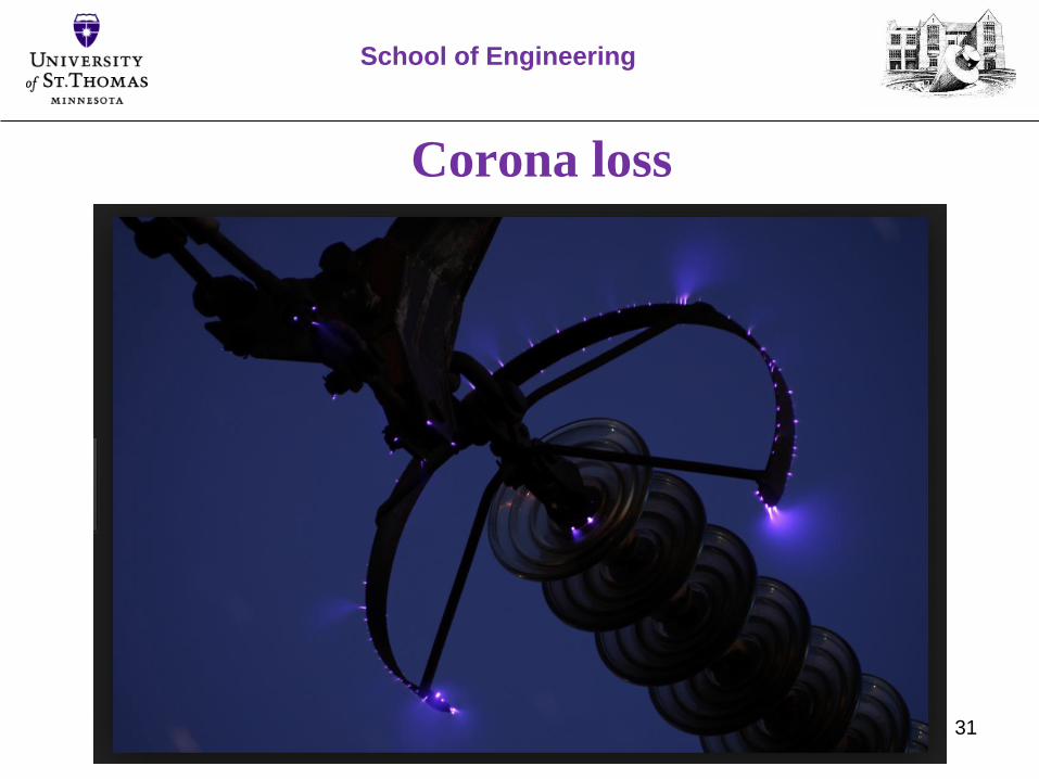
Corona loss


31

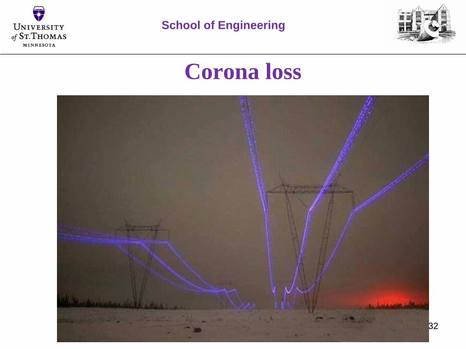
Corona loss


32

TL Parameters - Inductance


33


34

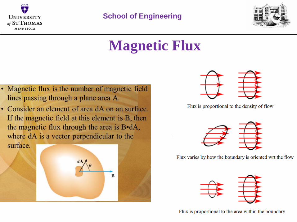
Inductance is defined by the ratio of the total magnetic flux flowing

through (passing through) an area divided by the current producing

that flux

Φ = S

B ∙ d 𝑠 ∝ 𝐼 , 𝑂𝑏𝑠𝑒𝑟𝑣𝑎𝑡𝑖𝑜𝑛

L =Φ

𝐼, 𝐷𝑒𝑓𝑖𝑛𝑖𝑡𝑖𝑜𝑛

Inductance is solely dependent on the geometry of the arrangement

and the magnetic properties (permeability ) of the medium.

Also, B = H where H is the mag field due to current flow only.

Magnetic Flux


35

Inductance

When a current flows through a conductor, a magnetic flux is set

up which links the conductor.

The current also establishes a magnetic field proportional to the

current in the wire.

Due to the distributed nature of a TL we are interested in the

inductance per unit length (H/m).


36

Inductance - Examples


37

Inductance of a Single Wire

The inductance of a magnetic circuit that has a constant permeability (𝜇) can be

obtained as follows:

The total magnetic field Bx at x via Amperes law:

𝐵𝑥 =𝜇𝑜 𝑥

2𝜋𝑟2𝐼 (𝑊𝑏/𝑚)

The flux d through slice dx is given by:

𝑑Φ = 𝐵𝑥 𝑑𝑎 = 𝐵𝑥 𝑙 𝑑𝑥 (𝑊𝑏)


38

The fraction of the current I in the wire that links the area da = dxl is:

Nf =x

r

2

The total flux through the wire is consequently given by:

Φ = 0

𝑟

𝑑Φ = 0

𝑟 𝑥

𝑟

2 𝜇𝑜 𝑥 𝐼

2𝜋𝑟2𝑙𝑑𝑥

Integrating with subsequent algebra to obtain inductance-per-m yields:

𝐿𝑤𝑖𝑟𝑒 −𝑠𝑒𝑙𝑓 = 0.5 ∙ 10−7 (𝐻/𝑚)


39


40

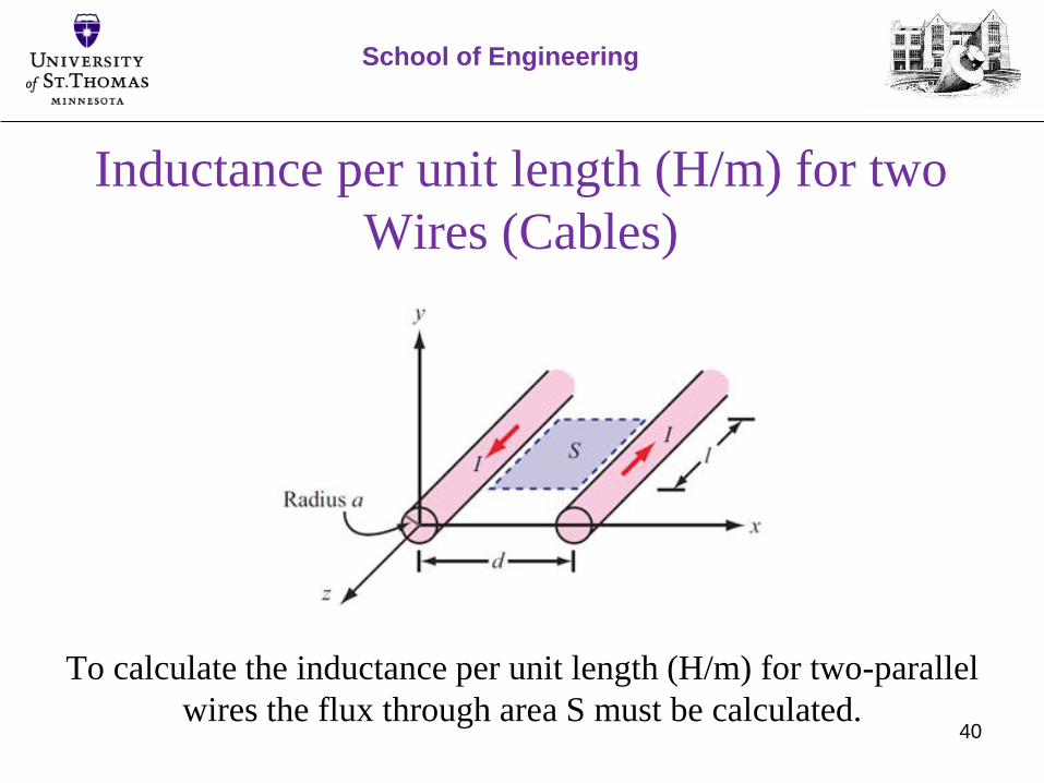
To calculate the inductance per unit length (H/m) for two-parallel

wires the flux through area S must be calculated.

Inductance per unit length (H/m) for two

Wires (Cables)

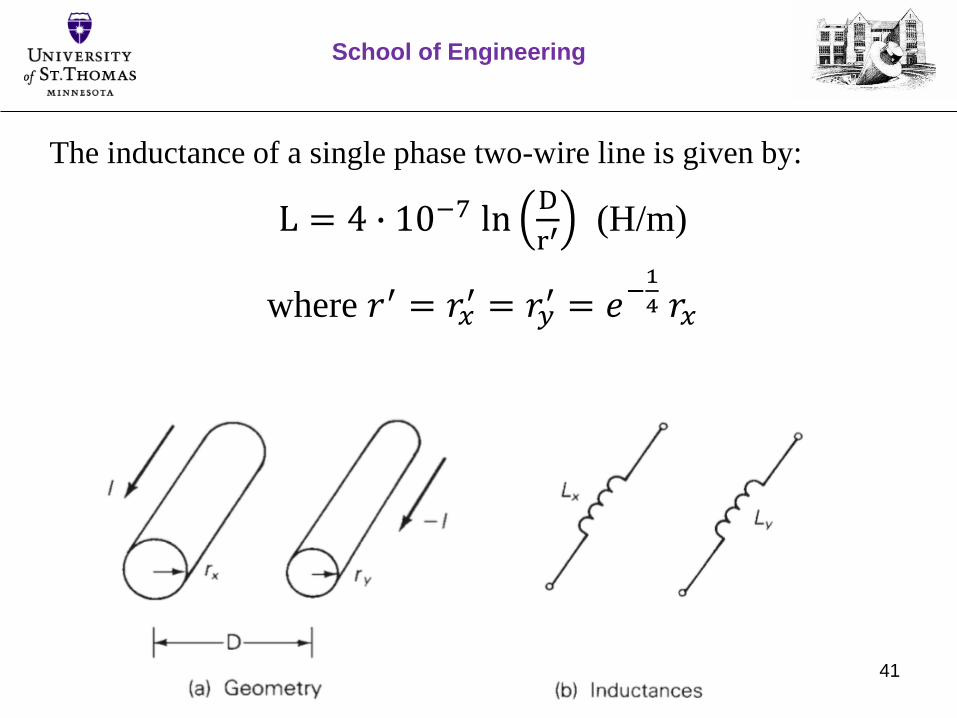
The inductance of a single phase two-wire line is given by:

L = 4 ∙ 10−7 lnD

r′(H/m)

where 𝑟′ = 𝑟𝑥′ = 𝑟𝑦′ = 𝑒−

1

4 𝑟𝑥


41

The inductance per phase of a 3-phase 3 wire line with equal spacing is given by:

La = 2 ∙ 10−7 ln

D

r′(H/m) per phase


42

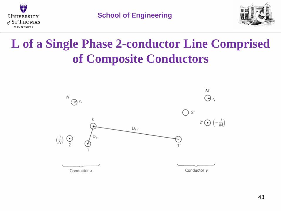
L of a Single Phase 2-conductor Line Comprised

of Composite Conductors


43

𝐿𝑥 = 2 ∙ 10−7 ln𝐷𝑥𝑦

𝐷𝑥𝑥

where

𝐷𝑥𝑦 =𝑀𝑁

𝑘=1

𝑁

𝑚=1′

𝑀

𝐷𝑘𝑚 𝑎𝑛𝑑 𝐷𝑥𝑥 =𝑁2

𝑘=1

𝑁

𝑚=1

𝑀

𝐷𝑘𝑚

Dxy is referred to as GMD = geometrical mean distance between conductors x & y

Dxx is referred to as GMR = geometrical mean radius of conductor x


44

A similar Ly express exists for conductor y.

LTotal = Lx + Ly (H/m)

Great NEWs!!!!!

Manufacturers often calculate these inductances for us for

various cable arrangements


45

Long 3-phase TLs are sometimes transposed for positive sequence balancing.

This is cleverly called ‘transposition’

The inductance (H/m) of a completely transposed three phase line may also be

calculated


46

𝐿𝑎 = 2 ∙ 10−7 ln𝐷𝑒𝑞

𝐷𝑠

𝐷𝑒𝑞 =3 𝐷12𝐷13𝐷23

La has units of (H/m)

Ds is the conductor GMR for stranded conductors or r’ for solid conductors


47

In HV TLs conductors are often arranged in one of the

following 3 standard configurations


48

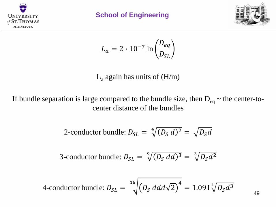
𝐿𝑎 = 2 ∙ 10−7 ln𝐷𝑒𝑞

𝐷𝑆𝐿

La again has units of (H/m)

If bundle separation is large compared to the bundle size, then Deq ~ the center-to-

center distance of the bundles

2-conductor bundle: 𝐷𝑆𝐿 =4𝐷𝑆 𝑑

2 = 𝐷𝑆𝑑

3-conductor bundle: 𝐷𝑆𝐿 =9𝐷𝑆 𝑑𝑑

3 =3𝐷𝑆𝑑2

4-conductor bundle: 𝐷𝑆𝐿 =16

𝐷𝑆 𝑑𝑑𝑑 24= 1.091

4𝐷𝑆𝑑3


49

TL Parameters - Capacitance


50


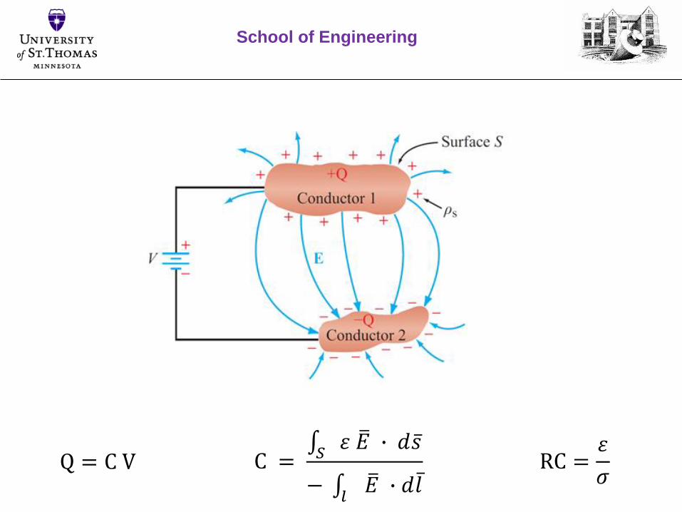
Q = C V C = 𝑆 𝜀 𝐸 ∙ 𝑑 𝑠

− 𝑙 𝐸 ∙ 𝑑 𝑙

RC =𝜀

𝜎

Capacitance

A capacitor results when any two conductors are separated by an insulating

medium.

Conductors of an overhead transmission line are separated by air – which acts

as an insulating medium – therefore they have capacitance.

Due to the distributed nature of a TL we are interested in the capacitance per

unit length (F/m).

Capacitance is solely dependent on the geometry of the arrangement and the

electric properties (permittivity ) of the medium


52

Calculating Capacitance

To calculate the capacitance between conductors we

must calculate two things:

The flux of the electric field E between the two conductors

The voltage V (electric potential) between the conductors

Then we take the ratio of these two quantities


53

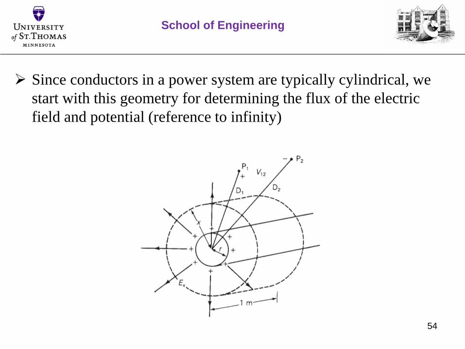
Since conductors in a power system are typically cylindrical, we

start with this geometry for determining the flux of the electric

field and potential (reference to infinity)


54

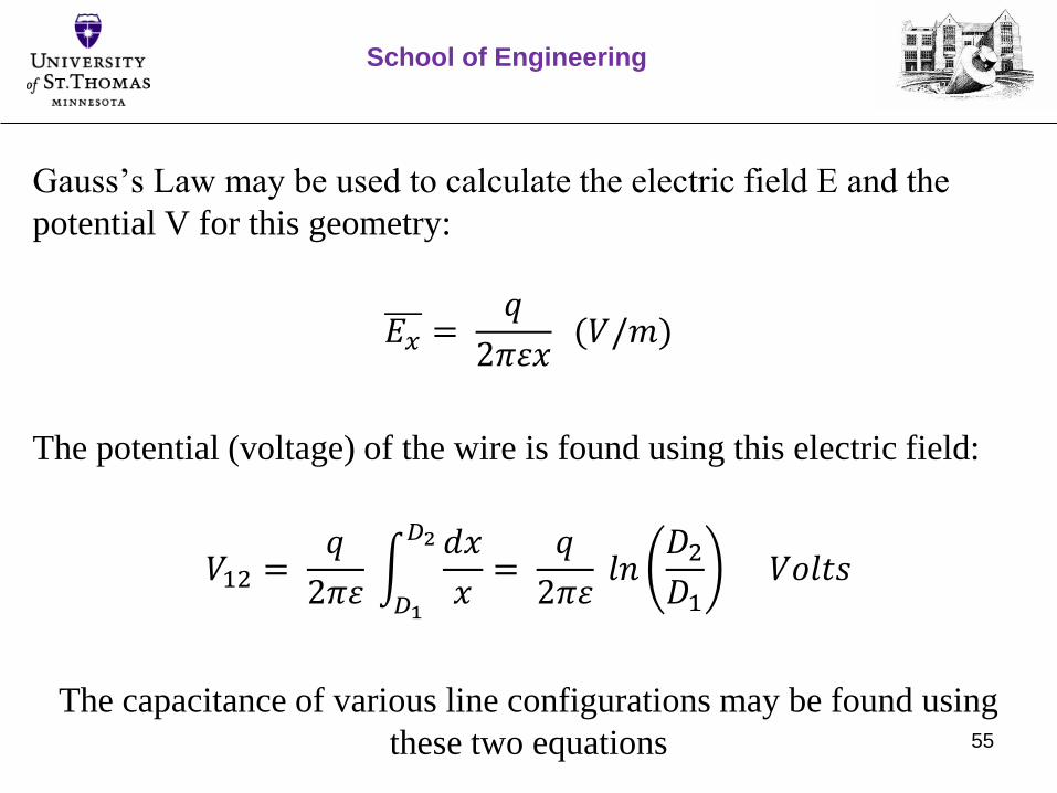
Gauss’s Law may be used to calculate the electric field E and the

potential V for this geometry:

𝐸𝑥 =𝑞

2𝜋𝜀𝑥(𝑉/𝑚)

The potential (voltage) of the wire is found using this electric field:

𝑉12 =𝑞

2𝜋𝜀 𝐷1

𝐷2 𝑑𝑥

𝑥=𝑞

2𝜋𝜀𝑙𝑛𝐷2𝐷1𝑉𝑜𝑙𝑡𝑠

The capacitance of various line configurations may be found using

these two equations


55

Capacitance - Examples


56

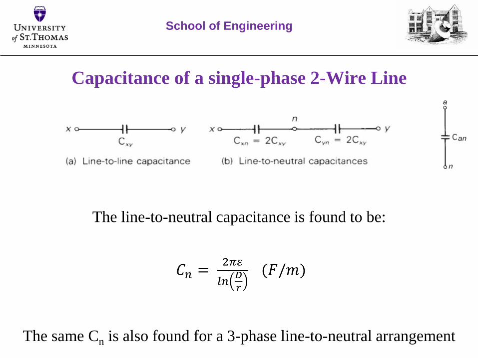
Capacitance of a single-phase 2-Wire Line

The line-to-neutral capacitance is found to be:

𝐶𝑛 =2𝜋𝜀

𝑙𝑛𝐷

𝑟

(𝐹/𝑚)

The same Cn is also found for a 3-phase line-to-neutral arrangement


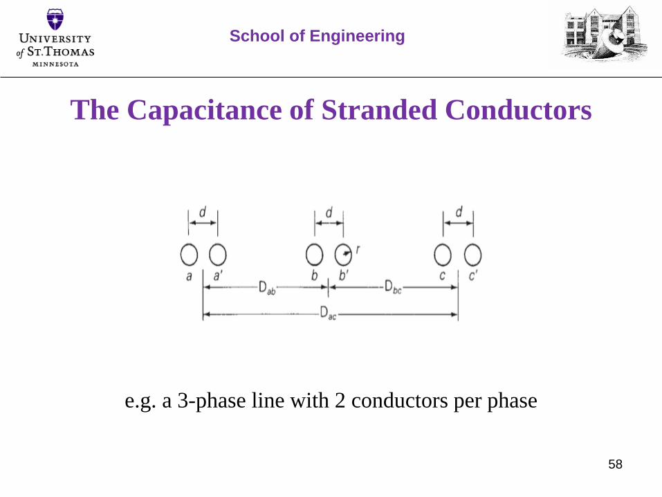
The Capacitance of Stranded Conductors

e.g. a 3-phase line with 2 conductors per phase


58

Direct analysis yields

𝐶𝑎𝑛 =2𝜋𝜀

𝑙𝑛𝐷𝑒𝑞𝑟

(𝐹/𝑚)

where

𝐷𝑒𝑞 =3 𝐷𝑎𝑏𝐷𝑎𝑐𝐷𝑏𝑐


59

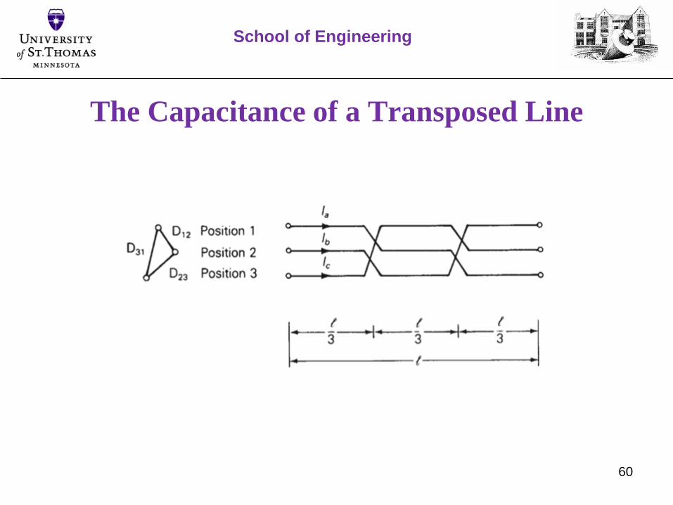
The Capacitance of a Transposed Line


60

The Capacitance of a Transposed Line

𝐶𝑎𝑛 =2𝜋𝜀

𝑙𝑛𝐷𝑒𝑞𝐷𝑆𝐶

(𝐹/𝑚)

where

𝐷𝑒𝑞 =3 𝐷𝑎𝑏𝐷𝑎𝑐𝐷𝑏𝑐

2-conductor bundle: 𝐷𝑆𝐶 = 𝑟 𝑑

3-conductor bundle: 𝐷𝑆𝐶 =3𝑟 𝑑2

4-conductor bundle: 𝐷𝑆𝐶 = 1.0914𝑟 𝑑3


61

TLs Continued


1

Dr. Greg Mowry

Annie Sebastian

Marian Mohamed

Maxwell’s Eqns. & the

Telegraph Eqns.


2

3


Maxwell’s Equations & Telegraph Equations

The ‘Telegrapher's Equations’ (or) ‘Telegraph Equations’ are a

pair of coupled, linear differential equations that describe the

voltage and current on a TL as functions of distance and time.

The original Telegraph Equations and modern TL model was

developed by Oliver Heaviside in the 1880’s.

The telegraph equations lead to the conclusion that voltages and

currents propagate on TLs as waves.


4

Maxwell’s Equations & Telegraph Equations

The Transmission Line equation can be derived using Maxwell’s

Equation.

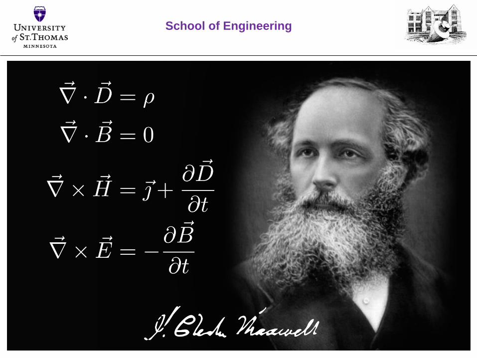
Maxwell's Equations (MEs) are a set of 4 equations that describe

all we know about electromagnetics.

MEs describe how electric and magnetic fields propagate, interact,

and how they are influenced by other objects.


5

Time for History

James Clerk Maxwell [1831-1879] was an Einstein/Newton-

level genius who took the set of known experimental laws

(Faraday's Law, Ampere's Law) and unified them into a

symmetric coherent set of Equations known as Maxwell's

Equations.

Maxwell was one of the first to determine the speed of

propagation of electromagnetic (EM) waves was the same as the

speed of light - and hence concluded that EM waves and visible

light were really descriptions of the same phenomena.


6

Maxwell’s Equations – 4 Laws

Gauss’ Law: The total of the electric flux through a closed surface

is equal to the charge enclosed divided by the permittivity. The

electric flux through an area is defined as the electric field

multiplied by the area of the surface projected in a plane

perpendicular to the field.

𝜵 ∙ 𝑫 =𝝆

𝝐

The ‘no name’ ME: The net magnetic flux through any closed

surface is zero.

𝛁 ∙ 𝑩 = 𝟎


7

Faraday’s law: Faraday's ‘law of induction’ is a basic law of

electromagnetism describing how a magnetic field interacts over a

closed path (often a circuit loop) to produce an electromotive force

(EMF; i.e. a voltage) via electromagnetic induction.

𝜵 𝑿 𝑬 = −𝝏 𝑩

𝝏𝒕

Ampere’s law: describes how a magnetic field is related to two

sources; (1) the current density J, and (2) the time-rate-of-change of

the displacement vector D.

𝜵 𝑿 𝑯 =𝝏 𝑫

𝝏𝒕+ 𝑱


8

The Constitutive Equations

Maxwell’s 4 equations are further augmented by the

‘constitutive equations’ that describe how materials interact with

fields to relate (B & H) and (D & E).

For simple linear, isotropic, and homogeneous materials the

constitutive equations are represented by:

𝑩 = 𝝁 𝑯 𝝁 = 𝝁𝒓 𝝁𝒐

𝑫 = 𝜺 𝑬 𝝐 = 𝜺𝒓 𝜺𝒐


9

The Telegraph Eqns.


10

11

TL Equations

TL equations can be derived by two methods:

Maxwell’s equations applied to waveguides

Infinitesimal analysis of a section of a TL operating in ACSS

with LCRG parameters (i.e. use phasors)

The TL circuit model is an infinite sequence of 2-port

components; each being an infinitesimally short

segment of the TL.


12

TL Equations

The LCRG parameters of a TL are expressed as per-

unit-length quantities to account for the experimentally

observed distributed characteristics of the TL

R’ = Conductor resistance per unit length, Ω/m

L’ = Conductor inductance per unit length, H/m

C’ = Capacitance per unit length between TL conductors, F/m

G’ = Conductance per unit length through the insulating medium between

TL conductors, S/m


13

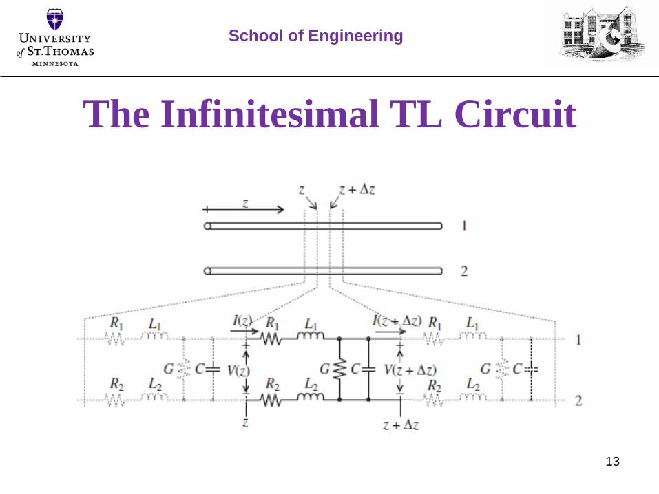
The Infinitesimal TL Circuit


14

The Infinitesimal TL Circuit Model


15

Transmission Lines Equations

The following circuit techniques and laws are used to

derive the lossless TL equations

KVL around the ‘abcd’ loop

KCL at node b

VL= L 𝜕i

𝜕tOLL for an inductor

IC= C 𝜕v

𝜕tOLC for a capacitor

Set 𝑅′= 𝐺′= 0 for the Lossless TL case


Apply KVL around the “abcd” loop:

𝑉(z) = V(z+∆z) +𝑅′∆z I(z) + 𝐿′∆z 𝜕𝐼(𝑧)

𝜕𝑡

Divide all the terms by ∆z :

𝑉 𝑧

∆𝑧=

𝑉 𝑧+∆𝑧

∆𝑧+ 𝑅′𝐼 𝑧 + 𝐿′

𝜕𝐼(𝑧)

𝜕𝑡

As ∆z 0 in the limit and R’ = 0 (lossless case):

𝜕𝑉(𝑧)

𝜕𝑧= – 𝑅′𝐼 𝑧 + 𝐿′

𝜕𝐼(𝑧)

𝜕𝑡

𝝏𝑽(𝒛)

𝝏𝒛= –𝑳′

𝝏𝑰(𝒛)

𝝏𝒕(Eq.1)


Apply KCL at node b:

𝐼(z) = I(z+∆z) +𝐺′∆z V(z+∆z) + 𝐶′∆z 𝜕𝑉(𝑧+∆𝑧)

𝜕𝑡

Divide all the terms by ∆z:

𝐼 𝑧

∆𝑧=

𝐼 𝑧+∆𝑧

∆𝑧+ 𝐺′𝑉 𝑧 + ∆𝑧 + 𝐶′

𝜕𝑉(𝑧+∆𝑧)

𝜕𝑡

As ∆z 0 in the limit and G’ = 0 (lossless case):

𝜕𝐼(𝑧)

𝜕𝑧= – 𝐺′𝑉 𝑧 + 𝐶′

𝜕𝑉(𝑧)

𝜕𝑡

𝝏𝑰(𝒛)

𝝏𝒛= – 𝑪′

𝝏𝑽(𝒛)

𝝏𝒕(Eq.2)


18

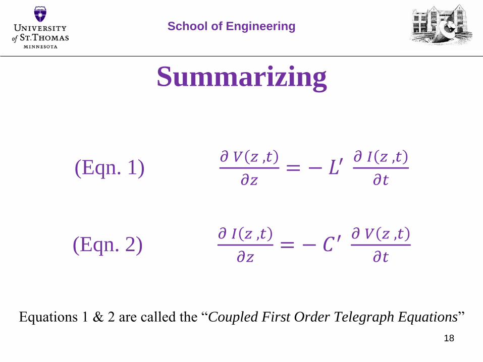
Summarizing

(Eqn. 1)𝜕 𝑉 𝑧 ,𝑡

𝜕𝑧= − 𝐿′

𝜕 𝐼 𝑧 ,𝑡

𝜕𝑡

(Eqn. 2)𝜕 𝐼 𝑧 ,𝑡

𝜕𝑧= − 𝐶′

𝜕 𝑉 𝑧 ,𝑡

𝜕𝑡


Equations 1 & 2 are called the “Coupled First Order Telegraph Equations”

Differentiating (Eq.1) wrt ‘z’ yields:

𝜕2𝑉(𝑧)

𝜕𝑧2= – 𝐿′

𝜕2𝐼(𝑧)

𝜕𝑧𝜕𝑡(Eq.3)

Differentiating (2) wrt ‘t’ yields:

𝜕2𝐼(𝑧)

𝜕𝑧𝜕𝑡= – 𝐶′

𝜕2𝑉(𝑧)

𝜕𝑡2(Eq.4)

Plugging equation 4 into 3:

𝝏𝟐𝑽(𝒛)

𝝏𝒛𝟐= 𝑳′𝑪′

𝝏𝟐𝑽(𝒛)

𝝏𝒕𝟐(Eq.5) 19


Differentiating (Eq.1) wrt ‘t’ yields:

𝜕2𝑉(𝑧)

𝜕𝑧𝜕𝑡= – 𝐿′

𝜕2𝐼(𝑧)

𝜕𝑡2(Eq.6)

Differentiating (2) wrt ‘z’ yields:

𝜕2𝐼(𝑧)

𝜕𝑧2= – 𝐶′

𝜕2𝑉(𝑧)

𝜕𝑧𝜕𝑡(Eq.7)

Plugging equation 6 into 7:

𝝏𝟐𝑰(𝒛)

𝝏𝒛𝟐= 𝑳′𝑪′

𝝏𝟐𝑰(𝒛)

𝝏𝒕𝟐(Eq.8)

20


Reversing the differentiation sequence

21

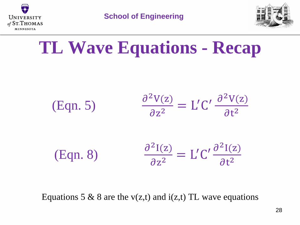
Summarizing

(Eqn. 5)𝜕2V(z)

𝜕z2= L′C′

𝜕2V(z)

𝜕t2

(Eqn. 8)𝜕2I(z)

𝜕z2= L′C′

𝜕2I(z)

𝜕t2


Equations 5 & 8 are the v(z,t) and i(z,t) TL wave equations

22

What is really cool about Equations 5 & 8 is that the solution to a

wave equation was already known; hence solving these equations

was straight forward.

The general solution of the wave equation has the following form:

f z, t = f(z ± ut)

where the ‘wave’ propagates with Phase Velocity 𝑢

u =ω

β=

ω

ω L′C′=

1

L′C′


23

The solution of the general wave equation, f(z,t), describes the

shape of the wave and has the following form:

f z, t = f(z − ut)

or

f z, t = f(z + ut)

The sign of 𝑢𝑡 determines the direction of wave propagation:

𝑓 𝑧 − 𝑢𝑡 Wave traveling in the +z direction

𝑓 𝑧 + 𝑢𝑡 Wave traveling in the –z direction


24

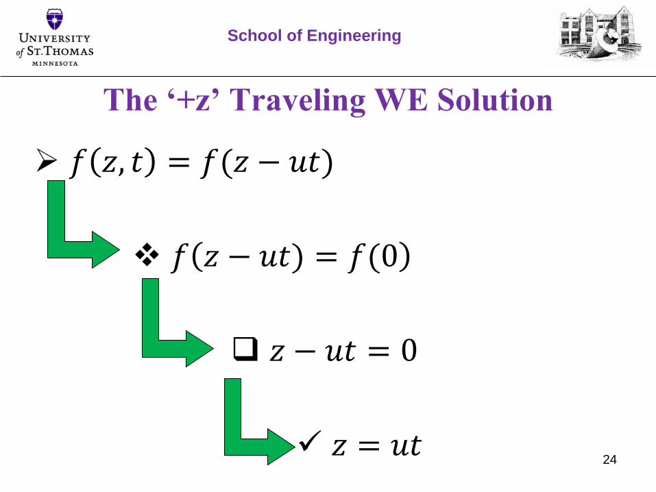
The ‘+z’ Traveling WE Solution

𝑓 𝑧, 𝑡 = 𝑓(𝑧 − 𝑢𝑡)

𝑓 𝑧 − 𝑢𝑡) = 𝑓(0

𝑧 − 𝑢𝑡 = 0

𝑧 = 𝑢𝑡


25

The argument of the wave equation solution is called the

phase.

Hence the culmination of all of this is that, “Waves

propagate by phase change”

One other key point, the form of the voltage WE and

current WE are identical. Hence solutions to each must

be of the same form and in phase.


26

Wave Equation z increases as t increase for a constant phase


TL Solutions


27

28

TL Wave Equations - Recap

(Eqn. 5)𝜕2V(z)

𝜕z2= L′C′

𝜕2V(z)

𝜕t2

(Eqn. 8)𝜕2I(z)

𝜕z2= L′C′

𝜕2I(z)

𝜕t2


Equations 5 & 8 are the v(z,t) and i(z,t) TL wave equations

29

ACSS TL Analysis Recipe


30

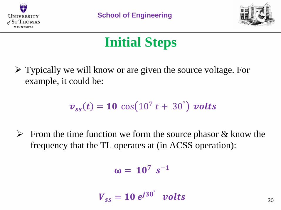
Initial Steps

Typically we will know or are given the source voltage. For

example, it could be:

𝒗𝒔𝒔 𝒕 = 𝟏𝟎 cos 107 𝑡 + 30° 𝒗𝒐𝒍𝒕𝒔

From the time function we form the source phasor & know the

frequency that the TL operates at (in ACSS operation):

𝛚 = 𝟏𝟎𝟕 𝒔−𝟏

𝑽𝒔𝒔 = 𝟏𝟎 𝒆𝒋𝟑𝟎°𝒗𝒐𝒍𝒕𝒔


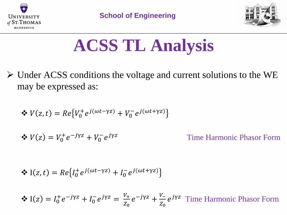
ACSS TL Analysis

Under ACSS conditions the voltage and current solutions to the WE

may be expressed as:

𝑉 𝑧, 𝑡 = 𝑅𝑒 𝑉0+𝑒𝑗(𝜔𝑡−γ𝑧) + 𝑉0

−𝑒𝑗(𝜔𝑡+γ𝑧)

𝑉 𝑧 = 𝑉0+𝑒−𝑗γ𝑧 + 𝑉0

−𝑒𝑗γ𝑧 Time Harmonic Phasor Form

I 𝑧, 𝑡 = 𝑅𝑒 𝐼0+𝑒𝑗(𝜔𝑡−γ𝑧) + 𝐼0

−𝑒𝑗(𝜔𝑡+γ𝑧)

I 𝑧 = 𝐼0+𝑒−𝑗γ𝑧 + 𝐼0

−𝑒𝑗γ𝑧 =𝑉+

𝑍0𝑒−𝑗γ𝑧 +

𝑉−

𝑍0𝑒𝑗γ𝑧 Time Harmonic Phasor Form


32

ACSS TL Analysis Recipe

Step 1: Assemble 𝑍0 , 𝑍𝐿, 𝑙, 𝑎𝑛𝑑 γ

Step 2: Determine Г𝐿

Step 3: Determine 𝑍𝑖𝑛

Step 4: Determine 𝑉𝑖𝑛

Step 5: Determine 𝑉0+

Step 6: Determine 𝑉𝐿

Step 7: Calculate 𝐼𝐿 and 𝑃𝐿


33

Step 1: Assemble 𝒁𝟎 , 𝒁𝑳, 𝒍, , and 𝜸

Characteristic Impedance:

𝒁𝒐 =𝑳′

𝑪′=

𝑽𝒐+

𝑰𝒐+ = −

𝑽𝒐−

𝑰𝒐−

Load Impedance:

𝒁𝑳 =𝑽𝑳𝑰𝑳

=𝑽𝟎+ + 𝑽𝟎

−

𝑽𝟎+ − 𝑽𝟎

− 𝒁𝟎

Complex Propagation Constant: ( = 0 for lossless TL)

𝜸 = 𝜶 + 𝒋𝜷 = 𝒋𝝎 𝑳′𝑪′


34

Additional Initial Results

Phase velocity uP:

𝐮𝐏 =𝛚

𝛃=

𝟏

𝐋′ 𝐂′

Identity:

𝐋′ 𝐂′ = 𝛍 𝛆


35

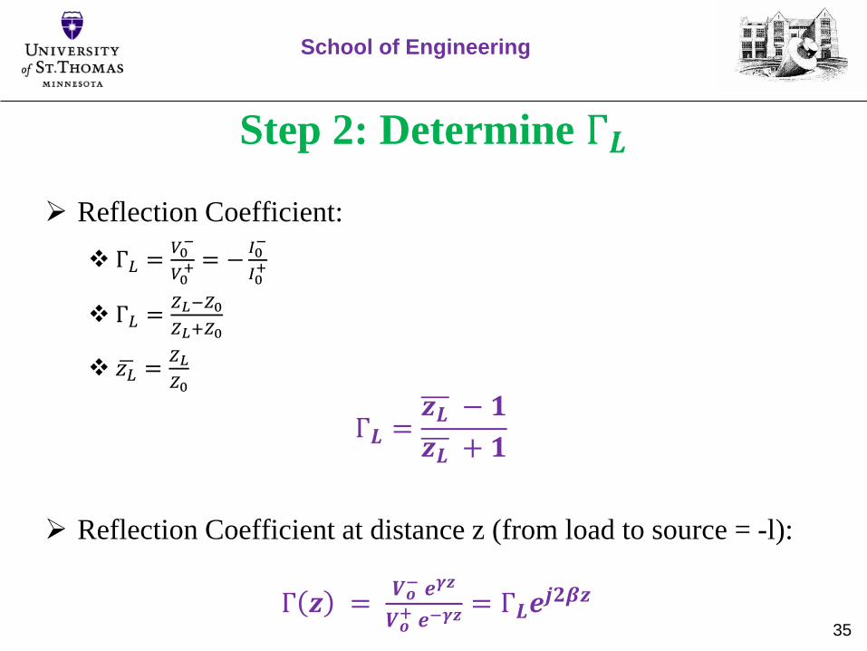
Step 2: Determine Г𝑳

Reflection Coefficient:

Г𝐿 =𝑉0−

𝑉0+ = −

𝐼0−

𝐼0+

Г𝐿 =𝑍𝐿−𝑍0

𝑍𝐿+𝑍0

𝑧𝐿 =𝑍𝐿

𝑍0

Г𝑳 =𝒛𝑳 − 𝟏

𝒛𝑳 + 𝟏

Reflection Coefficient at distance z (from load to source = -l):

Г 𝒛 =𝑽𝒐− 𝒆𝜸𝒛

𝑽𝒐+ 𝒆−𝜸𝒛

= Г𝑳𝒆𝒋𝟐𝜷𝒛


36

Additional Step-2 Results

VSWR:

𝐕𝐒𝐖𝐑 =𝟏 + 𝚪𝑳𝟏 − 𝚪𝑳

Range of the VSWR:

𝟎 < 𝑽𝑺𝑾𝑹 < ∞


37

Step 3: Determine 𝒁𝒊𝒏

Input Impedance:

𝒁𝒊𝒏 =𝑽𝒊𝒏 𝒛 = −𝒍

𝑰𝒊𝒏 𝒛 = −𝒍= 𝒁𝟎

𝒁𝑳 + 𝒁𝟎𝐭𝐚𝐧𝐡(𝜸𝒍)

𝒁𝟎 + 𝒁𝑳𝒕𝒂𝒏𝒉(𝜸𝒍)

For a lossless line tanh γl = j tan(βl):

𝒁𝒊𝒏 = 𝒁𝟎𝒁𝑳 + 𝒋𝒁𝟎𝒕𝒂𝒏(𝜷𝒍)

𝒁𝟎 + 𝒋𝒁𝑳𝒕𝒂𝒏(𝜷𝒍)

At any distance 𝑧1 from the load:

𝒁(𝒛𝟏) = 𝒁𝟎𝒁𝑳 + 𝒋𝒁𝟎𝐭𝐚𝐧(𝜷𝒛𝟏)

𝒁𝟎 + 𝒋𝒁𝑳𝒕𝒂𝒏(𝜷𝒛𝟏)


38

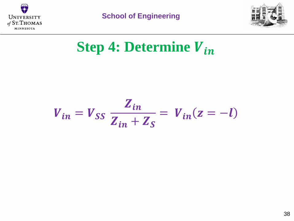
Step 4: Determine 𝑽𝒊𝒏

𝑽𝒊𝒏 = 𝑽𝑺𝑺𝒁𝒊𝒏

𝒁𝒊𝒏 + 𝒁𝑺= 𝑽𝒊𝒏 𝒛 = −𝒍


39

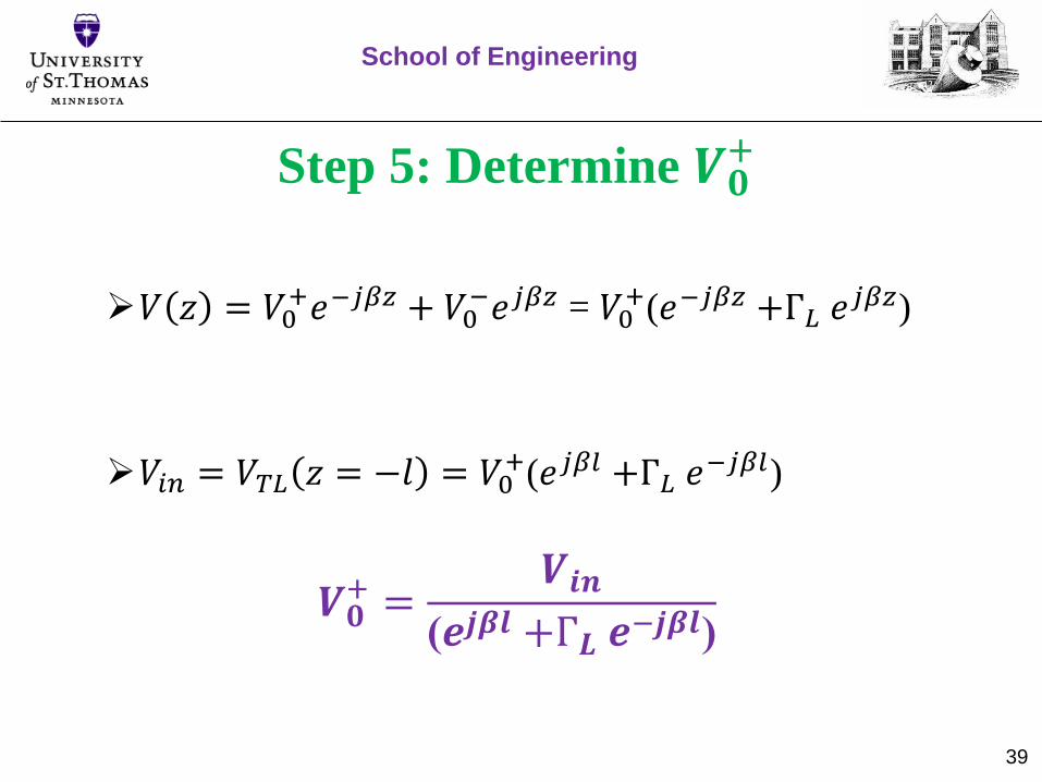
Step 5: Determine 𝑽𝟎+

𝑉 𝑧 = 𝑉0+𝑒−𝑗𝛽𝑧 + 𝑉0

−𝑒𝑗𝛽𝑧 = 𝑉0+(𝑒−𝑗𝛽𝑧 +Г𝐿 𝑒

𝑗𝛽𝑧)

𝑉𝑖𝑛 = 𝑉𝑇𝐿 𝑧 = −𝑙 = 𝑉0+(𝑒𝑗𝛽𝑙 +Г𝐿 𝑒

−𝑗𝛽𝑙)

𝑽𝟎+ =

𝑽𝒊𝒏(𝒆𝒋𝜷𝒍 +Г𝑳 𝒆

−𝒋𝜷𝒍)


40

Step 6: Determine 𝑽𝑳

Voltage at the load, VL:

𝑽𝑳 = 𝑽𝑻𝑳 𝒛 = 𝟎 = 𝑽𝒐+ 𝟏 + 𝚪𝑳

where:

𝑽𝟎+ =

𝑽𝒊𝒏(𝒆𝒋𝜷𝒍 +Г𝑳 𝒆

−𝒋𝜷𝒍)


41

Step 7: Calculate 𝑰𝑳 𝐚𝐧𝐝 𝑷𝑳

𝑰𝑳 =𝑽𝑳𝒁𝑳

𝑷𝒂𝒗𝒈 = 𝑷𝑳 =𝟏

𝟐𝑰𝑳𝟐𝑹𝒆(𝒁𝑳)

𝑰𝒏 𝒈𝒆𝒏𝒆𝒓𝒂𝒍, 𝑺𝑳 = 𝑽𝑳 𝑰𝑳∗ = 𝑷𝑳 + 𝒋 𝑸𝑳


42

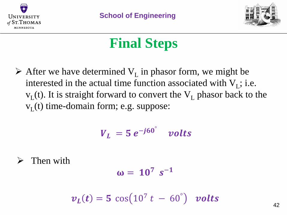
Final Steps

After we have determined VL in phasor form, we might be

interested in the actual time function associated with VL; i.e.

vL(t). It is straight forward to convert the VL phasor back to the

vL(t) time-domain form; e.g. suppose:

𝑽𝑳 = 𝟓 𝒆−𝒋𝟔𝟎°

𝒗𝒐𝒍𝒕𝒔

Then with

𝛚 = 𝟏𝟎𝟕 𝒔−𝟏

𝒗𝑳 𝒕 = 𝟓 cos 107 𝑡 − 60° 𝒗𝒐𝒍𝒕𝒔


43

Surge Impedance Loading (SIL)


Lossless TL with VS fixed for line-lengths < /4

2-Port Analysis


44

Two Port Network


45

A two-port network is an electrical ‘black box’

with two sets of terminals.

The 2-port is sometimes referred to as a four

terminal network or quadrupole network.

In a 2-port network, port 1 is often considered as

an input port while port 2 is considered to be an

output port.


46

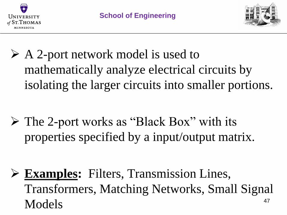
A 2-port network model is used to

mathematically analyze electrical circuits by

isolating the larger circuits into smaller portions.

The 2-port works as “Black Box” with its

properties specified by a input/output matrix.

Examples: Filters, Transmission Lines,

Transformers, Matching Networks, Small Signal

Models


47

Characterization of 2-Port Network

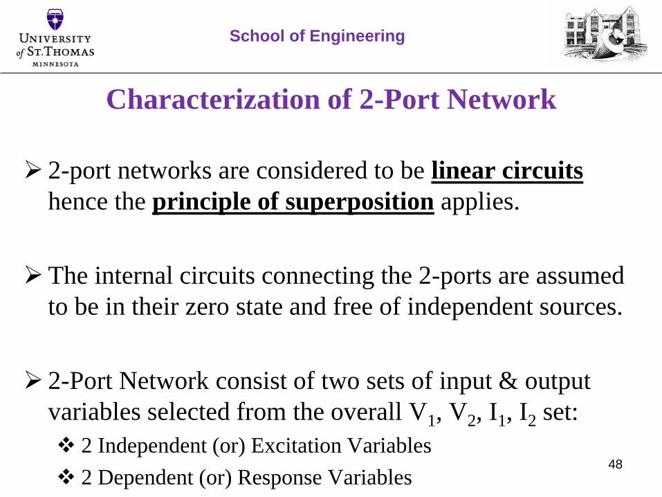
2-port networks are considered to be linear circuits

hence the principle of superposition applies.

The internal circuits connecting the 2-ports are assumed

to be in their zero state and free of independent sources.

2-Port Network consist of two sets of input & output

variables selected from the overall V1, V2, I1, I2 set:

2 Independent (or) Excitation Variables

2 Dependent (or) Response Variables


48

Characterization of 2-Port Network

Uses of 2-Port Network:

Analysis & Synthesis of Circuits and Networks.

Used in the field of communications, control system, power systems, and

electronics for the analysis of cascaded networks.

2-ports also show up in geometrical optics, wave-guides, and lasers

By knowing the matric parameters describing the 2-port network, it can be

considered as black-box when embedded within a larger network.


49

2-Port Networks & Linearity

Any linear system with 2 inputs and 2 outputs can always be

expressed as:

𝑦1𝑦2

=𝑎11 𝑎12𝑎21 𝑎22

𝑥1𝑥2


50

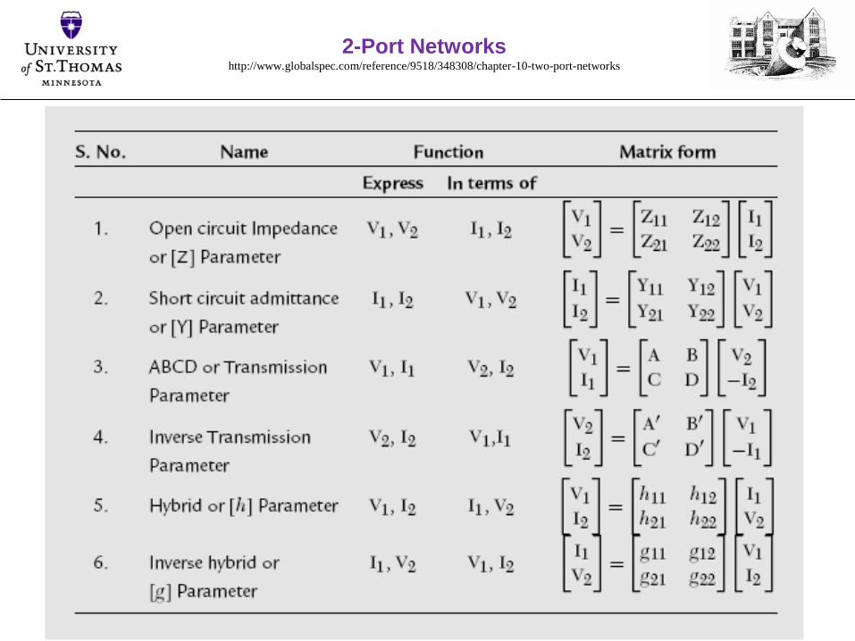
2-Port Networkshttp://www.globalspec.com/reference/9518/348308/chapter-10-two-port-networks

51

52

Review

A careful review of the preceding TL analysis reveals that all we

really determined in ACSS operation was Vin & Iin and VL & IL.

This reminds us of the exact input and output form of any linear

system with 2 inputs and 2 outputs which can always be

expressed as:

𝑦1𝑦2

=𝑎11 𝑎12𝑎21 𝑎22

𝑥1𝑥2

∴


Transmission Line as Two Port Network


ZS

+

-VS V1 = Vin V2 = VL

I1 = Iin I2 = IL

ZL

++

--

A B

C D

Source 2-Port Network Load

Representation of a TL by a 2-port network

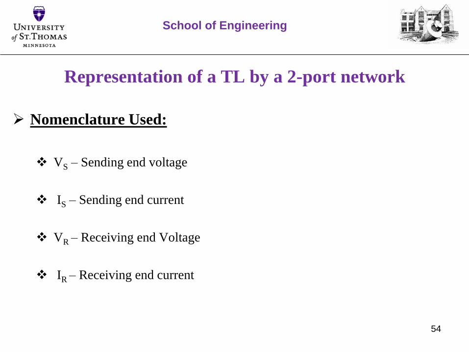
Nomenclature Used:

VS – Sending end voltage

IS – Sending end current

VR – Receiving end Voltage

IR – Receiving end current


54

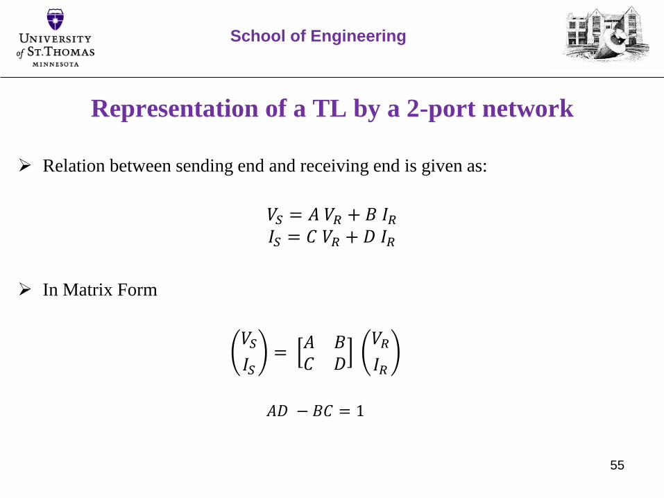
Representation of a TL by a 2-port network

Relation between sending end and receiving end is given as:

𝑉𝑆 = 𝐴 𝑉𝑅 + 𝐵 𝐼𝑅𝐼𝑆 = 𝐶 𝑉𝑅 + 𝐷 𝐼𝑅

In Matrix Form

𝑉𝑆𝐼𝑆

=𝐴 𝐵𝐶 𝐷

𝑉𝑅𝐼𝑅

𝐴𝐷 − 𝐵𝐶 = 1


55

56

4 Cases of Interest

Case 1: Short TL

Case 2: Medium distance TL

Case 3: Long TL

Case 4: Lossless TL


57

ABCD Matrix- Short Lines


58

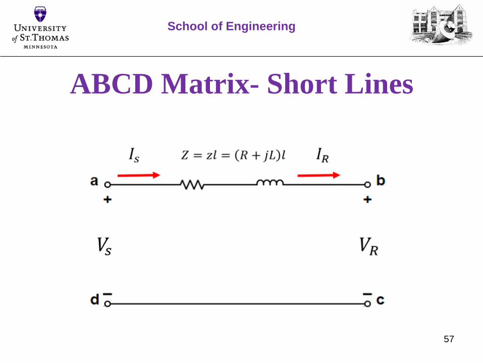
Short TL Less than ~80 Km

shunt Admittance is neglected

Apply KVL & KCL on abcd loop:

VS = VR + 𝑍IR

IS = IR

ABCD Matrix for short lines:

𝑉𝑆𝐼𝑆

=1 𝑍0 1

𝑉𝑅𝐼𝑅

ABCD Parameters:

A = D = 1 per unit

B = 𝑍 Ω

C = 0


ABCD Matrix- Medium Lines

59


60

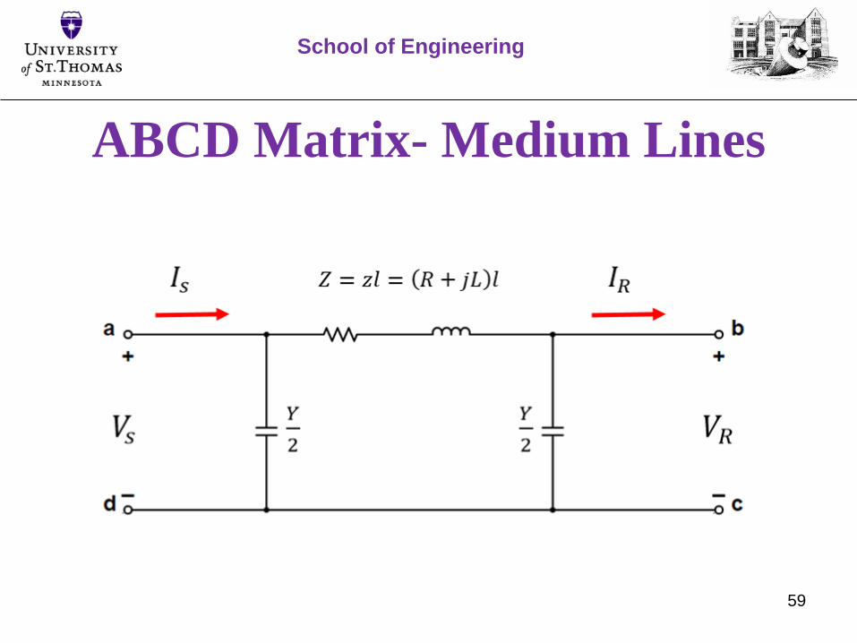
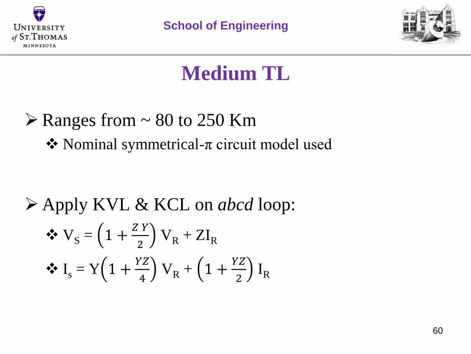
Medium TL

Ranges from ~ 80 to 250 Km

Nominal symmetrical-π circuit model used

Apply KVL & KCL on abcd loop:

VS = 1 +𝑍 𝑌

2VR + ZIR

Is = Y 1 +𝑌𝑍

4VR + 1 +

𝑌𝑍

2IR


61

Medium TL

ABCD Matrix for medium lines:

𝑉𝑆𝐼𝑆

=

1 +𝑌 𝑍

2𝑍

𝑌 1 +𝑌 𝑍

41 +

𝑌 𝑍

2

𝑉𝑅𝐼𝑅

ABCD Parameters:

A = D = 1 +𝑌𝑍

2per unit

B = Z Ω

C = Y 1 +𝑌𝑍

4Ω-1


ABCD Matrix- Long Lines

62


63

Long TL

More than ~ 250 Km and beyond

Full TL analysis

ZC = Z0

ABCD Matrix for long lines:

𝑉𝑆𝐼𝑆

=

cosh(𝛾𝑙) 𝑍𝐶 sinh(𝛾𝑙)1

𝑍𝐶sinh(𝛾𝑙) cosh(𝛾𝑙)

𝑉𝑅𝐼𝑅


64

ABCD Matrix- Lossless Lines R = G = 0

𝑍0 =𝐿′

𝐶′

γ = 𝑗ω 𝐿′𝐶′ = 𝑗β

ABCD Matrix for lossless lines:

𝑉𝑆𝐼𝑆

=

cos(𝛽𝑙) 𝑗 𝑍𝐶 sin(𝛽𝑙)𝑗

𝑍𝐶sin(𝛽𝑙) cos(𝛽𝑙)

𝑉𝑅𝐼𝑅

ABCD Parameters:

𝐴 = 𝐷 = cosh 𝛾𝑙 = cosh(𝑗β𝑙) = cos(β𝑙) per unit

𝐵 = 𝑍0 sinh γ𝑙 = 𝑗𝑍0sin(β𝑙) Ω

𝐶 =sinh(𝛾𝑙)

𝑍0= 𝑗

sin(𝛽𝑙)

𝑍0S


65

ABCD Matrix-Summary


A Brief Recipe on ‘How to do’

Power Flow Analysis (PFA)

Cooking with Dr. Greg Mowry


2

Steps

1. Represent the power system by its one-line diagram


3

Steps Cont.

2. Convert all quantities to per unit (pu)

2-Base pu analysis:

SBase kVA, MVA, …

VBase V, kV, …


4

Steps Cont.

3. Draw the impedance diagram


5

Steps Cont.

4. Determine the YBUS


6

Steps Cont.

5. Classify the Buses; aka ‘bus types’


7

Steps Cont.

6. Guess starting values for the unknown bus parameters;

e.g.


8

Steps Cont.

7. Using the power flow equations find approximations for the

real & reactive power using the initially guessed values and

the known values for voltage/angles/admittance at the

various buses. Find the difference in these calculated

values with the values that were actually given;

i.e. form P & Q.

(Δ value ) = (Given Value) – (Approximated Value)


9

Steps Cont.

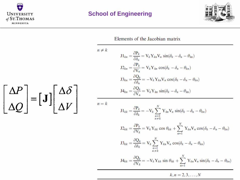
8. Write the Jacobian Matrix for the first iteration of the

Newton Raphson Method. This will have the form:

[Δvalues] = [Jacobian Matrix] * [ for Unknown Parameters]


10


11

Steps Cont.

9. Solve for the unknown differences by inverting the

Jacobian and multiplying & form the next guess:

(Unknown Value)new = (Unknown Value)old + Solved (Δ Value)


12

Steps Cont.

10. Repeat steps 7 – 9 iteratively until an accurate value for

the unknown differences as they 0. Then solve for all

the other unknown parameters.

Once these iterations converge (e.g. via NR), we now have

a fully solved power system with respect to Sj & Vj at all of

the system buses!!


1

Power Flow Analysis

(PFA)


Dr. Greg Mowry

Annie Sebastian

Marian Mohamed

2

Introduction


3

Power Flow Analysis

In modern power systems, bus voltages and power flow are controlled.

Power flow is proportional to v2, therefore controlling both bus voltage &

power flow is a nonlinear problem.

In power engineering, the power-flow study, or load-flow study, is a

numerical analysis of the flow of electric power in an interconnected system.

A power-flow study usually a steady-state analysis that uses simplified

notation such as a one-line diagram and per-unit system, and focuses on

various aspects of AC power parameters, such as voltages, voltage angles,

real power and reactive power.


4

Power Flow Analysis - Intro

PFA is very crucial during the power-system planning phases as well as

during periods of expansion and change for meeting present and future load

demands.

PFA is very useful (and efficient) at determining power flows and voltage

levels under normal operating conditions.

PFA provides insight into system operation and optimization of control

settings, which leads to maximum capacity at lower the operating costs.

PFA is typically performed under ACSS conditions for 3-phase power

systems


5

PFA Considerations

1. Generation Supplies the demand (load) plus losses.

2. Bus Voltage magnitudes remain close to rated values.

3. Gens Operate within specified real & reactive power limits

4. Transmission lines and Transformers are not overloaded.


6

Load Flow Studies (LFS)

Power-Flow or Load-Flow software (e.g. CYME, Power World, CAPE) is used

for investigating power system operations.

The SW determines the voltage magnitude and phase at each bus in a power

system under balanced three-phase steady state conditions.

The SW also computes the real and reactive power flows (P and Q

respectively) for all loads, buses, as well as the equipment losses.

The load flow is essential to decide the best operation of existing system, for

planning the future expansion of the system, and designing new power system.


7

LFS Requirements

Representation of the system by a one-line diagram.

Determining the impedance diagram using information in the one-

line diagram.

Formulation of network equations & PF equations.

Solution of these equations.


8

Conventional Circuit Analysis vs. PFA

Conventional nodal analysis is not suitable for power flow studies

as the input data for loads are normally given in terms of power

and not impedance.

Generators are considered power sources and not voltage or

current sources

The power flow problem is therefore formulated as a set of non-

linear algebraic equations that require numerical analysis for the

solution.


9

Bus

A ‘Bus’ is defined as the meeting point (or connecting

point) of various components.

Generators supply power to the buses and the loads

draw power from buses.

In a power system network, buses are considered as

nodes and hence the voltage is specified at each bus


The Basic 2-Bus AnalysisThe Foundational Heart of PFA

Quick Review


10

Motivation

The basic 2-Bus analysis must be understood by all

power engineers.

The 2-Bus analysis is effectively the ‘Thevenin

Equivalent” of all power systems and power flow

analysis.

Many variant exist, by my count, at least a dozen. We

will explore the basic 2-Bus PFA that models

transmission systems.


11

The Basic 2-Bus Power System


12

j X

+ -

I

𝑉𝑅 = 𝑉𝑅 ∠0° = 𝑉𝑅 𝑉𝑆 = 𝑉𝑆 ∠𝛿 = 𝑉𝑅𝑒

𝑗𝛿

1 2

S = ‘Send’ R = ‘Receive’

The Basic 2-Bus Power System


13

j X

+ -

I

𝑉𝑅 = 𝑉𝑅 ∠0° = 𝑉𝑅 𝑉𝑆 = 𝑉𝑆 ∠𝛿 = 𝑉𝑅𝑒

𝑗𝛿

1 2

~ ~

S = ‘Send’ R = ‘Receive’

2-Bus Phasor Diagram

VR the Reference


14

VRO

VS

I

90

j X I

j X I I due to j

Discussion

1) VS leads VR by

2) KVL VS – j X I = VR

∴ 𝐼 =𝑉𝑆 − 𝑉𝑅𝑗𝑋


15

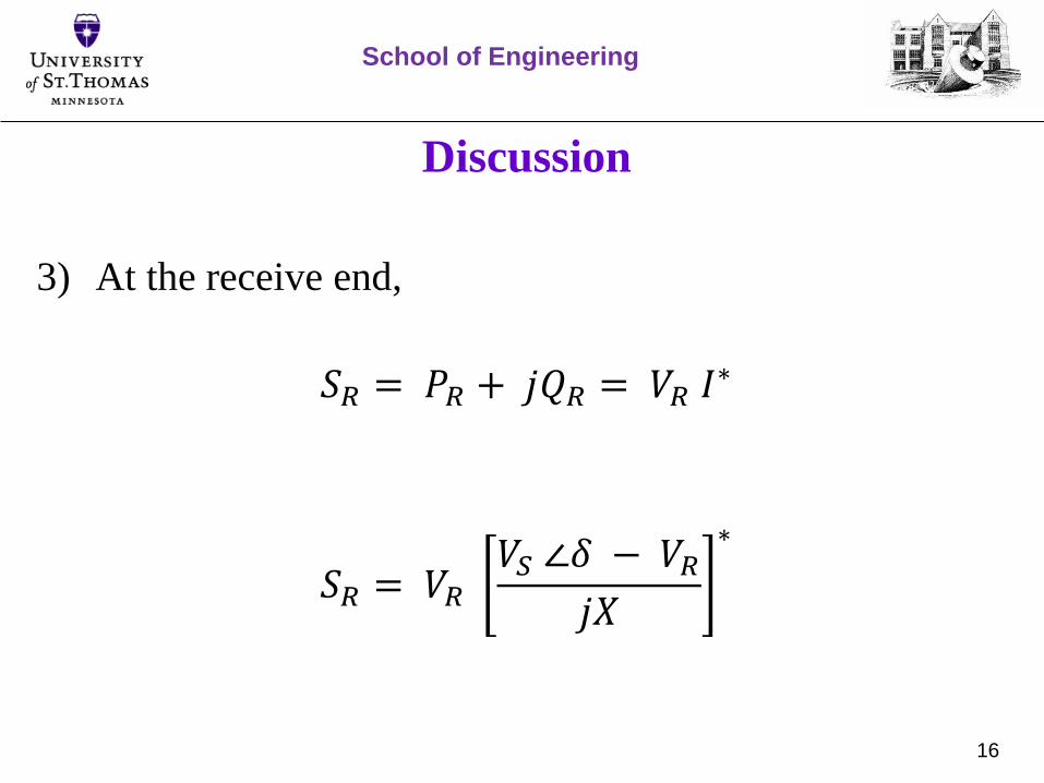
Discussion

3) At the receive end,

𝑆𝑅 = 𝑃𝑅 + 𝑗𝑄𝑅 = 𝑉𝑅 𝐼∗

𝑆𝑅 = 𝑉𝑅𝑉𝑆 ∠𝛿 − 𝑉𝑅𝑗𝑋

∗


16

Discussion

4) Therefore the complex power received is (after algebra):

𝑆𝑅 =𝑉𝑆 𝑉𝑅𝑋sin 𝛿 + 𝑗

𝑉𝑆 𝑉𝑅𝑋cos 𝛿 −

𝑉𝑅2

𝑋

𝑆𝑅 = 𝑃𝑅 + 𝑗𝑄𝑅

Recall 𝑉𝑆 = 𝑉𝑆∠𝛿 = 𝑉𝑆𝑒𝑗𝛿 = 𝑉𝑆 cos 𝛿 + 𝑗 sin 𝛿


17

Discussion

5) Or:

𝑃𝑅 =𝑉𝑆 𝑉𝑅𝑋sin 𝛿

𝑄𝑅 =𝑉𝑆 𝑉𝑅𝑋cos 𝛿 −

𝑉𝑅2

𝑋


18

Discussion

6) Note that if VS ~ VR ~ V then:

𝑃𝑅 ≈𝑉2

𝑋𝛿

𝑄𝑅 ≈𝑉

𝑋∆𝑉


19

20

2-Bus, Y, and PFA Lead-in


21

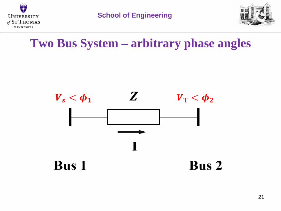
Two Bus System – arbitrary phase angles


22

Two Bus System

The complex AC power flow at the receiving end bus can be calculated as

follows:

𝑺𝒓 = 𝑽𝒓 𝑰∗

Similarly, the power flow at the sending end bus is:

𝑺𝒔 = 𝑽𝒔 𝑰∗

where

𝑉𝑠 = 𝑉𝑠 𝑒𝑗𝜑1 is the voltage and phase angle at the sending bus.

𝑉𝑟 = 𝑉𝑟 𝑒𝑗𝜑2 is the voltage and phase angle at the receiving bus.

Z is the complex impedance of the TL.


23

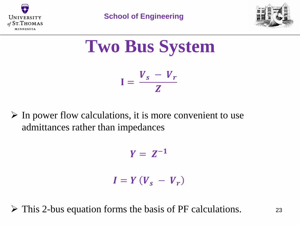
Two Bus System

𝐈 =𝑽𝒔 − 𝑽𝒓𝒁

In power flow calculations, it is more convenient to use

admittances rather than impedances

𝒀 = 𝒁−𝟏

𝑰 = 𝒀 𝑽𝒔 − 𝑽𝒓

This 2-bus equation forms the basis of PF calculations.


24

The Admittance Matrix

The use of admittances greatly simplifies PFA

e.g. an open circuit between two buses (i.e. no connection) results in Y = 0

(which is computationally easy to deal with) rather than Z = ∞ (which is

computationally hard to deal with).

Vij is the voltage at bus i wrt bus j; bus i positive, bus j negative

Iab represents the current flow from bus a to bus b

Recall that a ‘node voltage’ (bus voltage) is the voltage at that node (Bus) with

respect to the reference.


25

Admittance Matrix Method (1)

NV analysis results in n-1 node equations (bus equations) which is

analytically very efficient for systems with large n.

Given systems with n large, an efficient and automatable method is

needed/required for PFA. NVM and Y-matrix methods are so.

In circuit analysis, series circuit elements are typically combined to

form a single impedance to simplify the analysis. This is generally

not done in PFA.


26

Admittance Matrix Method (2)

In PFA, combining series elements is not typically done as we seek to keep track

of the impedances of various assets and their power flows; e.g. in:

i. Generators

ii. TLs

iii. XFs

iv. FACTs

Voltages sources (e.g. generators) have an associated impedance (the Thevenin

impedance) that is typically inductive in ACSS


27

Y-Matrix Example


28

Example Circuit


29

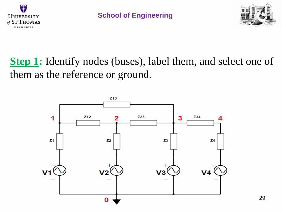
Step 1: Identify nodes (buses), label them, and select one of

them as the reference or ground.


30

Step 2 & 3: (2) Replace voltage sources and their Thevenin

impedance with their Norton equivalent. (3) Replace

impedance with their associated admittances.


31

Step 4: Form the system matrix

𝒀𝑩𝒖𝒔 ∗ 𝑽 = 𝑰 (Eqn-1)

where,

Ybus = Bus Admittance matrix of order (n x n); known

V = Bus (node) voltage matrix of order (n x 1); unknown

I = Source current matrix of order (n x 1); known


32

Step 5: Solve the system matrix for bus voltages

𝑽 = 𝒀𝑩𝒖𝒔−𝟏 ∗ 𝑰 (Eqn-2)

Note: at this point the various known bus voltages (amplitude and

phase) may be used to calculate currents and power flow.


33

Stuffing the Y-Matrix

Y-matrix elements are designated as 𝑌𝑘𝑛 where k refers to the kth bus

and n refers to the nth bus.

Diagonal elements 𝑌𝑘𝑘:

𝑌𝑘𝑘 = sum of all of the admittances connected to the kth bus

Off-diagonal elements 𝑌𝑘𝑛:

𝑌𝑘𝑛 = 𝑌𝑛𝑘 = -(sum of the admittances in the branch connecting bus k to bus n)


34

Y-Matrix Terminology

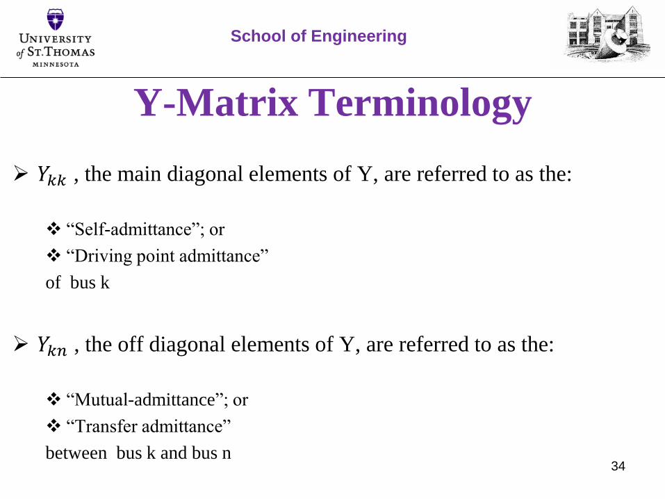
𝑌𝑘𝑘 , the main diagonal elements of Y, are referred to as the:

“Self-admittance”; or

“Driving point admittance”

of bus k

𝑌𝑘𝑛 , the off diagonal elements of Y, are referred to as the:

“Mutual-admittance”; or

“Transfer admittance”

between bus k and bus n


35

Y-Matrix Notes

If there is no connection between bus k and bus n, then 𝑌𝑘𝑛 = 0 in

the Y-matrix; hence there are 2 zeros in the Y-matrix for this

situation since 𝑌𝑘𝑛 = 𝑌𝑛𝑘.

If a new connection is made between 2 buses k & n in a network,

then only 4 elements of the Y matrix change, all of the others remain

the same. The elements that change are:

𝑌𝑘𝑘 𝑌𝑛𝑛 𝑌𝑘𝑛 = 𝑌𝑛𝑘


36

The ‘stuffed’ Y-Matrix

I1I2I3I4

=

Y11 Y12 Y13 0Y21 Y22 Y23 0

Y310Y320

Y33Y43

Y34Y44

V1V2V3V4

Note that since no direct connections exist between Bus 1 & 4 or Bus 2 & 4,

the corresponding entries in the Y matrix are zero


37

Y-Matrix Math


38

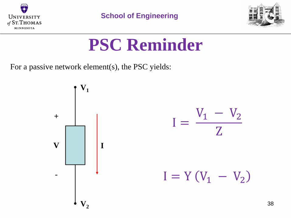
PSC ReminderFor a passive network element(s), the PSC yields:


I

+

V

-

I =V1 − V2Z

V2

V1

I = Y V1 − V2

39

Y-Matrix Equations

Consider the following bus in a network:


I3

V1

Bus 3

V2

V3

Z23

Z13

Ic

Ia

Ib

Id

ZC1

ZC2

40

Y-Matrix EquationsKCL at bus 3 yields:

𝐈𝟑 = 𝐈𝐛 + 𝐈𝐝 + 𝐈𝐚 + 𝐈𝐜

𝑰𝟑 =𝑽𝟑𝒁𝑪𝟏+𝑽𝟑𝒁𝑪𝟐+𝑽𝟑 − 𝑽𝟏𝒁𝟏𝟑

+𝑽𝟑 − 𝑽𝟐𝒁𝟐𝟑

𝑰𝟑 = 𝑽𝟑 𝒀𝟑,𝒕𝒐𝒕𝒂𝒍 𝒕𝒐 𝒈𝒏𝒅 +

𝒎≠ 𝟑

𝑽𝟑 − 𝑽𝒎𝒁𝒎𝟑


41

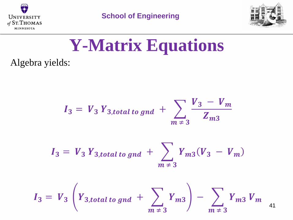
Y-Matrix EquationsAlgebra yields:


𝒎≠ 𝟑

𝑽𝟑 − 𝑽𝒎𝒁𝒎𝟑


𝒎≠ 𝟑

𝒀𝒎𝟑 𝑽𝟑 − 𝑽𝒎


𝒎≠ 𝟑

𝒀𝒎𝟑 −

𝒎≠ 𝟑

𝒀𝒎𝟑 𝑽𝒎


42

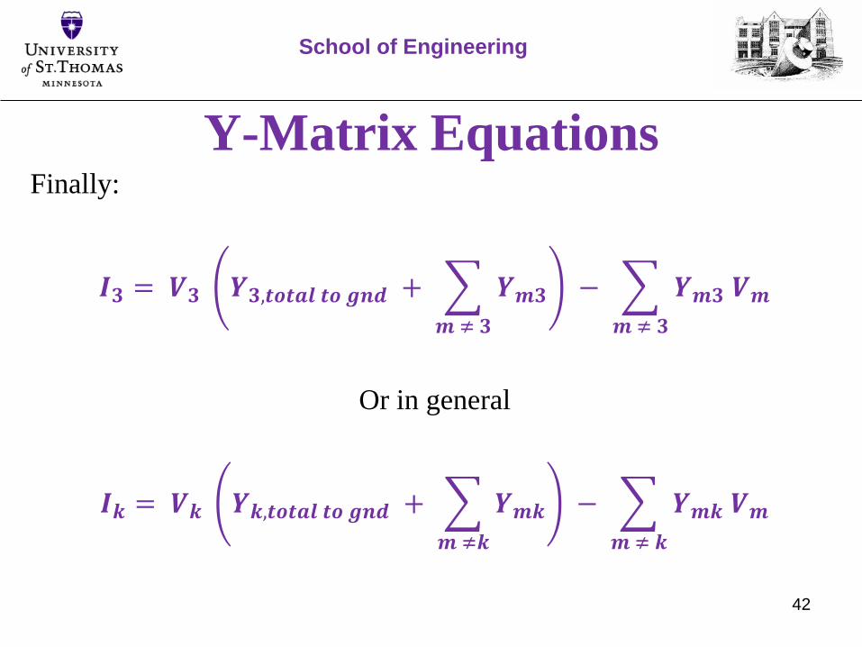
Y-Matrix EquationsFinally:


𝒎≠ 𝟑

𝒀𝒎𝟑 −

𝒎≠ 𝟑

𝒀𝒎𝟑 𝑽𝒎

Or in general

𝑰𝒌 = 𝑽𝒌 𝒀𝒌,𝒕𝒐𝒕𝒂𝒍 𝒕𝒐 𝒈𝒏𝒅 +

𝒎≠𝒌

𝒀𝒎𝒌 −

𝒎≠ 𝒌

𝒀𝒎𝒌 𝑽𝒎


43

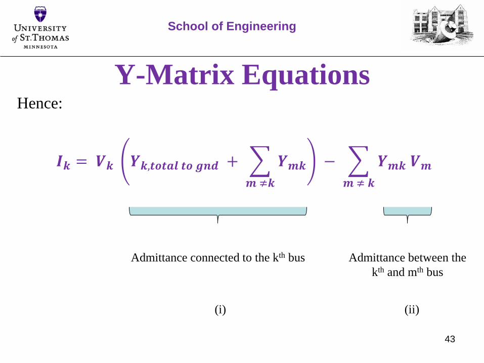
Y-Matrix EquationsHence:

𝑰𝒌 = 𝑽𝒌 𝒀𝒌,𝒕𝒐𝒕𝒂𝒍 𝒕𝒐 𝒈𝒏𝒅 +

𝒎≠𝒌

𝒀𝒎𝒌 −

𝒎≠ 𝒌

𝒀𝒎𝒌 𝑽𝒎


Admittance connected to the kth bus Admittance between the

kth and mth bus

(i) (ii)

44

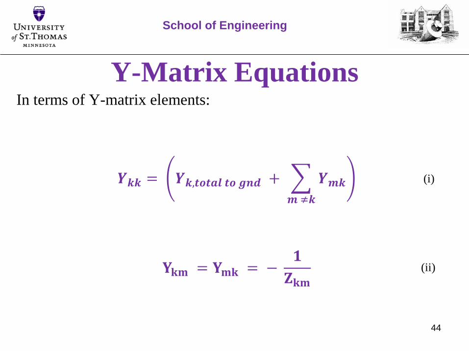
Y-Matrix EquationsIn terms of Y-matrix elements:

𝒀𝒌𝒌 = 𝒀𝒌,𝒕𝒐𝒕𝒂𝒍 𝒕𝒐 𝒈𝒏𝒅 +

𝒎≠𝒌

𝒀𝒎𝒌

𝐘𝐤𝐦 = 𝐘𝐦𝐤 = −𝟏

𝐙𝐤𝐦


(i)

(ii)

45

Y-Matrix EquationsUsing the short-hand notation:

𝑰𝒌 = 𝑽𝒌 𝒀𝒌𝒌 +

𝒎≠ 𝒌

𝑽𝒎 𝒀𝒎𝒌

𝐘𝐤𝐦 = 𝐘𝐦𝐤


46

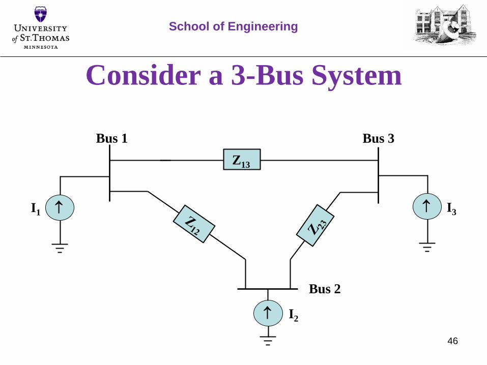
Consider a 3-Bus System


I3

Bus 3

Z13

Bus 2

Bus 1

I2

I1

47

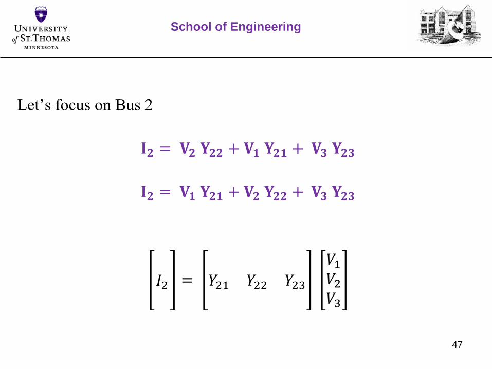
Let’s focus on Bus 2

𝐈𝟐 = 𝐕𝟐 𝐘𝟐𝟐 + 𝐕𝟏 𝐘𝟐𝟏 + 𝐕𝟑 𝐘𝟐𝟑

𝐈𝟐 = 𝐕𝟏 𝐘𝟐𝟏 + 𝐕𝟐 𝐘𝟐𝟐 + 𝐕𝟑 𝐘𝟐𝟑

𝐼2 = 𝑌21 𝑌22 𝑌23

𝑉1𝑉2𝑉3


48

The General Case

For a n-Bus system we have:

𝐼1⋮𝐼𝑛

=𝑌11 ⋯ 𝑌1𝑛⋮ ⋱ ⋮𝑌𝑛1 ⋯ 𝑌𝑛𝑛

𝑉1⋮𝑉𝑛


To be calculatedKnown sources The Y-Matrix

49

Power Flow Equations


50

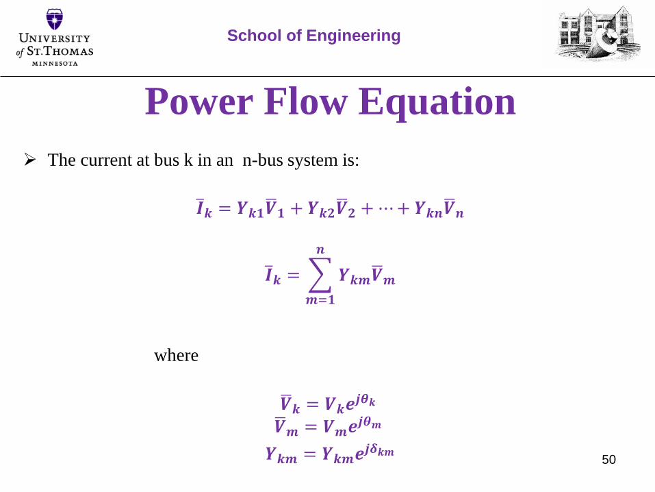
Power Flow Equation

The current at bus k in an n-bus system is:

𝑰𝒌 = 𝒀𝒌𝟏 𝑽𝟏 + 𝒀𝒌𝟐 𝑽𝟐 +⋯+ 𝒀𝒌𝒏 𝑽𝒏

𝑰𝒌 =

𝒎=𝟏

𝒏

𝒀𝒌𝒎 𝑽𝒎

where

𝑽𝒌 = 𝑽𝒌𝒆𝒋𝜽𝒌

𝑽𝒎 = 𝑽𝒎𝒆𝒋𝜽𝒎

𝒀𝒌𝒎 = 𝒀𝒌𝒎𝒆𝒋𝜹𝒌𝒎


51

The complex power S at bus k is given by:

𝑺𝒌 = 𝑽𝒌 𝑰𝒌∗ = 𝑷𝒌 + 𝒋𝑸𝒌

𝑺𝒌 = 𝑽𝒌

𝒎=𝟏

𝒏

𝒀𝒌𝒎 𝑽𝒎

∗


Power Flow Equation

52

Substituting the voltage and admittance phasors into the complex power

equations yields:

𝐒𝐤 = 𝐏𝐤 + 𝐣𝐐𝐤 = 𝐕𝐤𝐞𝐣𝛉𝐤

𝐦= 𝟏

𝐧

𝐘𝐤𝐦𝐞𝐣𝛅𝐤𝐦 𝐕𝐦𝐞

𝐣𝛉𝐦

∗

By Euler’s Theorem

𝑽𝒌 𝑽𝒎∗= 𝑽𝒌 𝑽𝒎 𝐜𝐨𝐬 𝜽𝒌𝒎 + 𝒋 𝐬𝐢𝐧 𝜽𝒌𝒎

where 𝜽𝒌𝒎 = 𝜽𝒌 − 𝜽𝒎


Power Flow Equation

53

Expanding the complex power summation into real and imaginary parts and

associating these with P & Q respectively yields our fundamental PFA equations

𝑷𝒌 =

𝒎= 𝟏

𝒏

𝑽𝒌 𝑽𝒎 𝒀𝒌𝒎 𝐜𝐨𝐬 𝜽𝒌 − 𝜽𝒎 + 𝜹𝒌𝒎

𝑸𝒌 =

𝒎= 𝟏

𝒏

𝑽𝒌 𝑽𝒎 𝒀𝒌𝒎 𝐬𝐢𝐧 𝜽𝒌 − 𝜽𝒎 + 𝜹𝒌𝒎


Power Flow Equation

54

Key SUMMARY points:

The bus voltage equations, I=YV, are linear

The power flow equations are quadratic, V2 appears in all P & Q terms

Consequently simultaneously controlling bus voltage and power flow is a non-

linear problem

In general this forces us to use numerical solution methods for solving the

power flow equations while controlling bus voltages


Power Flow Equation

55

Network Terminology


56

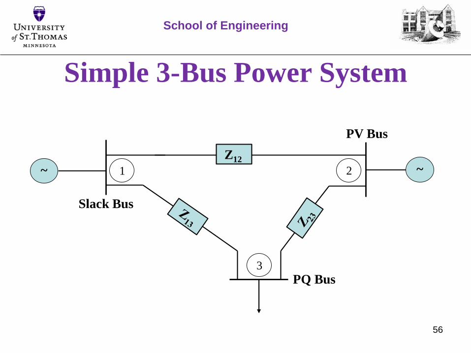
Simple 3-Bus Power System


PV Bus

Z12

PQ Bus

Slack Bus

~ ~1 2

3

57

Bus Types


Bus TypeTotal number of

buses

Quantities

Specified

Quantities to be

obtained

Load Bus (or)

PQ Busn-m P, Q V , δ

Generator Bus (or)

Voltage Controlled

Bus (or)

PV Bus

m-1 P, V Q , δ

Slack Bus (or)

Swing Bus (or)

Reference Bus

1 V , δ P, Q

58

Bus Terminology

P = PG – PD

Q = QG – QD

PG & QG are the Real and Reactive Power supplied by the power system

generators connected

PD & QD are respectively the Real and Reactive Power drawn by bus loads

V = Magnitude of Bus Voltage

δ = Phase angle of Bus Voltage


59

The Need for a Slack Bus

TL losses can be estimated only if the real and reactive power at all

buses are known.

The powers in the buses will be known only after solving the load

flow equations.

For these reasons, the real and reactive power of one of the

generator bus is not specified.

This special bus is called Slack Bus and serves as the system

reference and power balancing agent.


60

The Need for a Slack Bus

It is assumed that the Slack Bus Generates the real and reactive

power of the Transmission Line losses.

Hence for a Slack Bus, the magnitude and phase of bus voltage are

specified and real and reactive powers are obtained through the

load flow equation.

𝑺𝒖𝒎 𝒐𝒇 𝑪𝒐𝒎𝒑𝒍𝒆𝒙𝑷𝒐𝒘𝒆𝒓 𝒐𝒇 𝑮𝒆𝒏𝒆𝒓𝒂𝒕𝒐𝒓

= 𝑺𝒖𝒎 𝒐𝒇 𝑪𝒐𝒎𝒑𝒍𝒆𝒙𝑷𝒐𝒘𝒆𝒓 𝒐𝒇 𝑳𝒐𝒂𝒅𝒔

+ 𝑻𝒐𝒕𝒂𝒍 𝑪𝒐𝒎𝒑𝒍𝒆𝒙 𝑷𝒐𝒘𝒆𝒓𝒍𝒐𝒔𝒔 𝒊𝒏 𝑻𝒓𝒂𝒏𝒔𝒎𝒊𝒔𝒔𝒊𝒐𝒏 𝑳𝒊𝒏𝒆𝒔

or

𝑻𝒐𝒕𝒂𝒍 𝑪𝒐𝒎𝒑𝒍𝒆𝒙 𝒑𝒐𝒘𝒆𝒓𝒍𝒐𝒔𝒔 𝒊𝒏 𝑻𝒓𝒂𝒏𝒔𝒎𝒊𝒔𝒔𝒊𝒐𝒏 𝑳𝒊𝒏𝒆𝒔

= 𝑺𝒖𝒎 𝒐𝒇 𝑪𝒐𝒎𝒑𝒍𝒆𝒙𝑷𝒐𝒘𝒆𝒓 𝒐𝒇 𝑳𝒐𝒂𝒅𝒔

-𝑺𝒖𝒎 𝒐𝒇 𝑪𝒐𝒎𝒑𝒍𝒆𝒙𝑷𝒐𝒘𝒆𝒓 𝒐𝒇 𝑮𝒆𝒏𝒆𝒓𝒂𝒕𝒐𝒓


61

Solving the PF equations


62

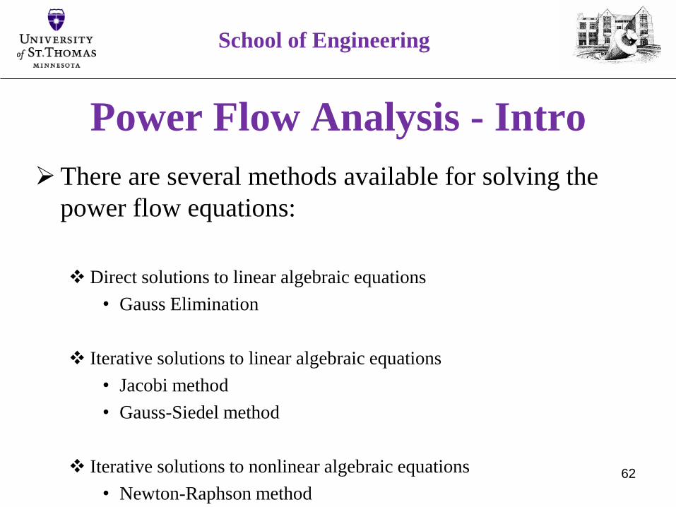
Power Flow Analysis - Intro

There are several methods available for solving the

power flow equations:

Direct solutions to linear algebraic equations

• Gauss Elimination

Iterative solutions to linear algebraic equations

• Jacobi method

• Gauss-Siedel method

Iterative solutions to nonlinear algebraic equations

• Newton-Raphson method


63

Gauss-Seidel Method

In numerical linear algebra, the Gauss–Seidel method, also known as the Liebmann method

or the method of successive displacement, is an iterative method used to solve a linear system

of equations. It is named after the German mathematicians Carl Friedrich Gauss and Philipp

Ludwig von Seidel, and is similar to the Jacobi method. Though it can be applied to any

matrix with non-zero elements on the diagonals, convergence is only guaranteed if the matrix

is either diagonally dominant, or symmetric and positive definite. It was only mentioned in a

private letter from Gauss to his student Gerling in 1823.


64

The Jacobi Method

Carl Gustav Jacob Jacobi was a German mathematician,

who made fundamental contributions to elliptic functions,

dynamics, differential equations, and number theory.


Newton-Raphson Method

65


In numerical analysis, Newton's method (also known as the Newton–Raphson method),

is named after Isaac Newton and Joseph Raphson. It is a method for finding

successively better approximations to the roots (or zeroes) of a real-valued function.

𝐱; 𝐟 𝐱 = 𝟎

The Newton–Raphson method in one variable is implemented as follows:

The method starts with a function f defined over the real numbers x

The function's derivative f',

An initial guess x0 for a root of the function f.

If the function is ‘well behaved’ then a better approximation to the actual root is x1:

𝒙𝟏 = 𝒙𝟎 −𝐟(𝒙𝟎)

𝐟′(𝒙𝟎)66



67

The Newton-Raphson method is a very popular non-

linear equation solver as:

NR is very powerful and typically converges very quickly

Almost all PFA SW uses Newton-Raphson

Very forgiving when errors are made in one iterations; the final

solution will be very close to the actual root



68

Procedure:

Step 1: Assume a vector of initial guess x(0) and set iteration counter k = 0

Step 2: Compute f1(x(k)), f2(x

(k)),⋯⋯ fn(x(k))

Step 3: Compute ∆𝑚1, ∆𝑚2, ⋯⋯ Δ𝑚𝑛.

Step 4: Compute error = max[ ∆𝑚1 , ∆𝑚2 ,⋯⋯ ∆𝑚𝑛 ]

Step 5: If error ≤ ∈ (pre-specified tolerance), then the final solution vector is x(k)

and print the results. Otherwise go to step 6

Step 6: Form the Jacobin matrix analytically and evaluate it at x = x(k)

Step 7: Calculate the correction vector ∆𝑥 = [∆𝑚1, ∆𝑚2, ⋯⋯ Δ𝑚𝑛]T by using

equation d

Step 8: Update the solution vector x(k+1) = x(k) + ∆𝑥 and update k=k+1 and go back

to step 2.



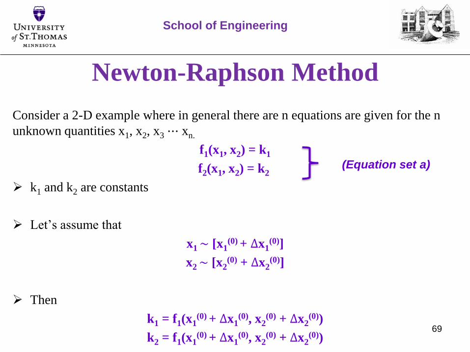
69

Consider a 2-D example where in general there are n equations are given for the n

unknown quantities x1, x2, x3⋯ xn.

f1(x1, x2) = k1

f2(x1, x2) = k2

k1 and k2 are constants

Let’s assume that

x1~ [x1(0) + ∆x1

(0)]

x2~ [x2(0) + ∆x2

(0)]

Then

k1 = f1(x1(0) + ∆x1

(0), x2(0) + ∆x2

(0))

k2 = f1(x1(0) + ∆x1

(0), x2(0) + ∆x2

(0))


(Equation set a)


70

Applying the first order Taylor Expansion to f1 and f2

k1≅ f1(x1(0), x2

(0)) +∆x1(0) 𝝏𝒇𝟏𝝏𝒙𝟏

+ ∆x2(0) 𝝏𝒇𝟏𝝏𝒙𝟐

k2≅ f2(x1(0), x2

(0)) +∆x1(0) 𝝏𝒇𝟐𝝏𝒙𝟏

+ ∆x2(0) 𝝏𝒇𝟐𝝏𝒙𝟐

‘Equation set b’ expressed in matrix form,

k1− f1(x1(0), x2

(0))

k2− f2(x1(0), x2

(0))=

𝝏𝒇𝟏𝝏𝒙𝟏

𝝏𝒇𝟏𝝏𝒙𝟐

𝝏𝒇𝟐𝝏𝒙𝟏

𝝏𝒇𝟐𝝏𝒙𝟐

∆x1(0)

∆x2(0)


(Equation set b)

(Equation c)

The Baby Jacobian

Matrix


71

Then

∆k1(0)

∆k2(0) = J(0)

∆x1(0)

∆x2(0)

Adjusting the guess according to

x1(1) = [x1

(0) + ∆x1(0)]

x2(1) = [x2

(0) + ∆x2(0)]

Iterate until ∆xi(N) < ∈



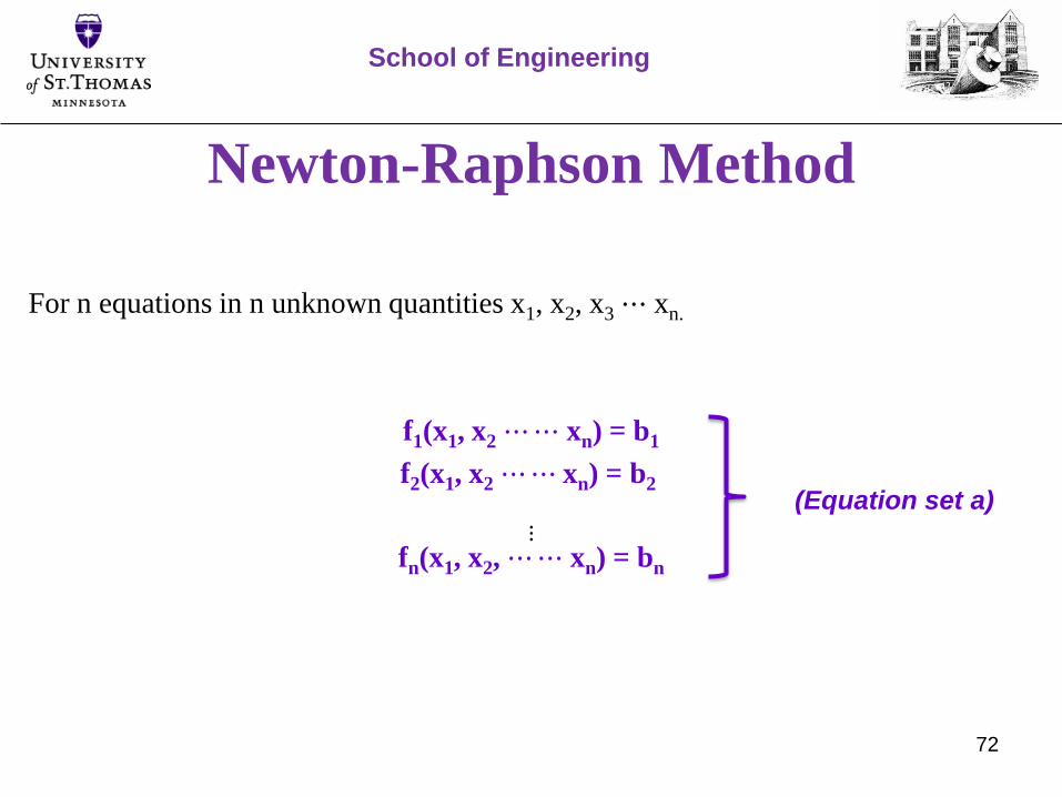
72

For n equations in n unknown quantities x1, x2, x3⋯ xn.

f1(x1, x2⋯⋯ xn) = b1

f2(x1, x2⋯⋯ xn) = b2

⋮fn(x1, x2, ⋯⋯ xn) = bn


(Equation set a)


73

In ‘equation set a’ the quantities b1, b2, ⋯ bn as well as the functions f1, f2⋯⋯fn

are known.

To solve the equation set an initial guess is made; the initial guesses be denoted

as x1(0), x2

(0), ⋯ xn(0).

First order Taylor’s series expansions (neglecting the higher order terms) are

carried out for these equation about the initial guess

The vector of initial guesses is denoted as x(0) = [x1(0), x2

(0), ⋯ xn(0)]T.

Applying Taylor’s expansion to the “equation set a” will give:



74

f1(x1(0), x2

(0) ⋯⋯ xn(0)) +

𝝏𝒇𝟏

𝝏𝒙𝟏

∆𝒙𝟏+𝝏𝒇𝟏

𝝏𝒙𝟐

∆𝒙𝟐 + ⋯+𝝏𝒇𝟏

𝝏𝒙𝒏∆𝒙𝒏 = b1

f2(x1(0), x2

(0) ⋯⋯ xn(0)) +

𝝏𝒇𝟐

𝝏𝒙𝟏

∆𝒙𝟏+𝝏𝒇𝟐

𝝏𝒙𝟐

∆𝒙𝟐 + ⋯+𝝏𝒇𝟐

𝝏𝒙𝒏∆𝒙𝒏 = b2

⋮

fn(x1(0), x2

(0) ⋯⋯ xn(0)) +

𝝏𝒇𝒏

𝝏𝒙𝟏

∆𝒙𝟏 +𝝏𝒇𝒏

𝝏𝒙𝟐

∆𝒙𝟐 + ⋯+𝝏𝒇𝟐

𝝏𝒙𝒏∆𝒙𝒏 = bn

‘Equation set b’ can be written in matrix form as:

𝒇𝟏(𝒙𝟎)

𝒇𝟐(𝒙𝟎)

⋮𝒇𝒏(𝒙

𝟎)

=

𝝏𝒇𝟏

𝝏𝒙𝟏

𝝏𝒇𝟏

𝝏𝒙𝟐

⋯𝝏𝒇𝟏

𝝏𝒙𝒏𝝏𝒇𝟐

𝝏𝒙𝟏

𝝏𝒇𝟐

𝝏𝒙𝟐

⋯𝝏𝒇𝟐

𝝏𝒙𝒏

⋮𝝏𝒇𝒏

𝝏𝒙𝟏

𝝏𝒇𝒏

𝝏𝒙𝟐

⋯𝝏𝒇𝒏

𝝏𝒙𝒏

∆𝒙𝟏∆𝒙𝟐

⋮∆𝒙𝒏

=

𝒃𝟏𝒃𝟐

⋮𝒃𝒏


(Equation set b)

(Equation c)

75

𝝏𝒇𝟏

𝝏𝒙𝟏

𝝏𝒇𝟏

𝝏𝒙𝟐

⋯𝝏𝒇𝟏

𝝏𝒙𝒏𝝏𝒇𝟐

𝝏𝒙𝟏

𝝏𝒇𝟐

𝝏𝒙𝟐

⋯𝝏𝒇𝟐

𝝏𝒙𝒏

⋮𝝏𝒇𝒏

𝝏𝒙𝟏

𝝏𝒇𝒏

𝝏𝒙𝒏⋯𝝏𝒇𝒏

𝝏𝒙𝒏

Hence ‘equation c’ can be written as

∆𝒙𝟏∆𝒙𝟐

⋮∆𝒙𝒏

= [J-1]

𝒃𝟏 − 𝒇𝟏(𝒙𝟎)

𝒃𝟐 − 𝒇𝟐(𝒙𝟎)

⋮𝒃𝒏 − 𝒇𝒏(𝒙

𝟎)

= [J-1]

∆𝒎𝟏∆𝒎𝟐

⋮∆𝒎𝒏

‘Equation d’ is the basic equation for solving the n algebraic equations given in

‘equation set a’.


Jacobin Matrix (J)

(Equation d)

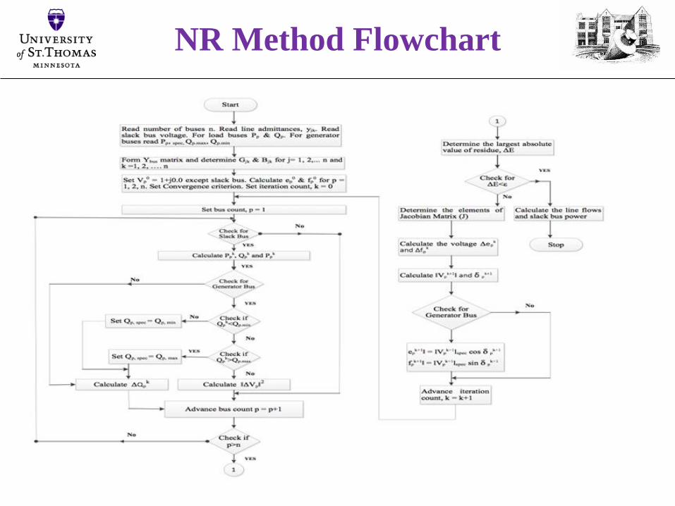
76

NR Method Flowchart

77

Power Flow Example(using Power World)


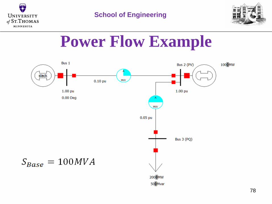
78

Power Flow Example


79

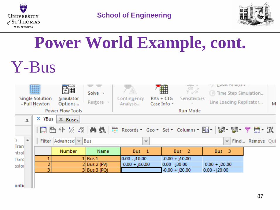
Step 1: Calculate Y-Bus:

YBus =

−𝑗10 𝑗10 0

𝑗100

−𝑗30𝑗20

𝑗20−𝑗20


Power Flow Example, cont.

80

Step 2: Define Bus types and their quantities:



Bus No Bus TypeQuantities

Specified

Quantities to be

obtained

One Slack Bus 𝑉1 , δ1 ---

TwoGenerator Bus

PV𝑃2 , 𝑉2 δ2 , 𝑄2

ThreeLoad Bus

PQ 𝑃3 , 𝑄3 𝑉3 , δ3

81

Step 3: User Power Equations to solve for unknowns:

𝑷𝟐 =

𝒎= 𝟏

𝟑

𝑽𝟐 𝑽𝒎 𝒀𝟐𝒎 𝐜𝐨𝐬 𝜽𝟐𝒌 − 𝜹𝟐 + 𝜹𝒎

𝑷𝟑 =

𝒎= 𝟏

𝟑

𝑽𝟑 𝑽𝒎 𝒀𝟑𝒎 𝐜𝐨𝐬 𝜽𝟑𝒌 − 𝜹𝟑 + 𝜹𝒎

𝑸𝟑 = −

𝒎= 𝟏

𝟑

𝑽𝟑 𝑽𝒎 𝒀𝟑𝒎 𝐬𝐢𝐧 𝜽𝟑𝒌 − 𝜹𝟑 + 𝜹𝒎



82

𝟏 = 𝟏𝟎 𝒔𝒊𝒏𝜹𝟐 − 𝟐𝟎 𝑽𝟑 𝒔𝒊𝒏(−𝜹𝟐+𝜹𝟑) Eq.1

𝟐 = 𝟐𝟎 𝑽𝟑 𝒔𝒊𝒏(−𝜹𝟑+𝜹𝟐) Eq.2

𝟎. 𝟓 = 𝟐𝟎 𝑽𝟑 𝒄𝒐𝒔 −𝜹𝟑+𝜹𝟐 − 𝟐𝟎 𝑽𝟑𝟐

Eq.3



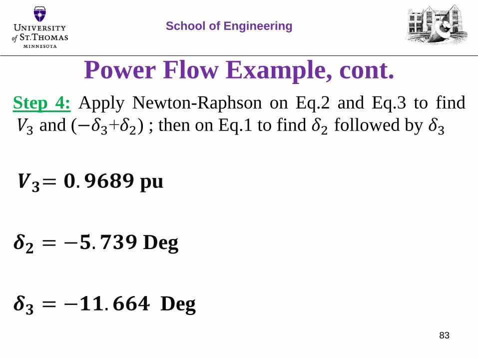
83

Step 4: Apply Newton-Raphson on Eq.2 and Eq.3 to find

𝑉3 and (−𝛿3+𝛿2) ; then on Eq.1 to find 𝛿2 followed by 𝛿3

𝑽𝟑= 𝟎. 𝟗𝟔𝟖𝟗 pu

𝜹𝟐 = −𝟓. 𝟕𝟑𝟗 Deg

𝜹𝟑 = −𝟏𝟏. 𝟔𝟔𝟒 Deg



84

Step 5: Use 𝑽𝟑, 𝜹𝟐, and 𝜹𝟑 to find 𝑸𝟐 and 𝑸𝟏:

𝑸𝟐 = −

𝒎=𝟏

𝟑

𝑽𝟐 𝑽𝒎 𝒀𝟐𝒎 𝐬𝐢𝐧 𝜽𝟐𝒌 − 𝜹𝟐 + 𝜹𝒎

𝑸𝟏 = −

𝒎=𝟏

𝟑

𝑽𝟏 𝑽𝒎 𝒀𝟏𝒎 𝐬𝐢𝐧 𝜽𝟏𝒌 − 𝜹𝟏 + 𝜹𝒎

𝑸𝟐 = 𝟎. 𝟕𝟕𝟔 pu

𝑸𝟐 = 𝟎. 𝟕𝟕𝟔 pu



85

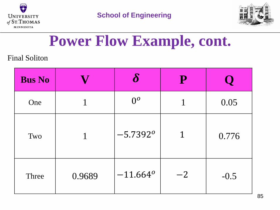
Final Soliton



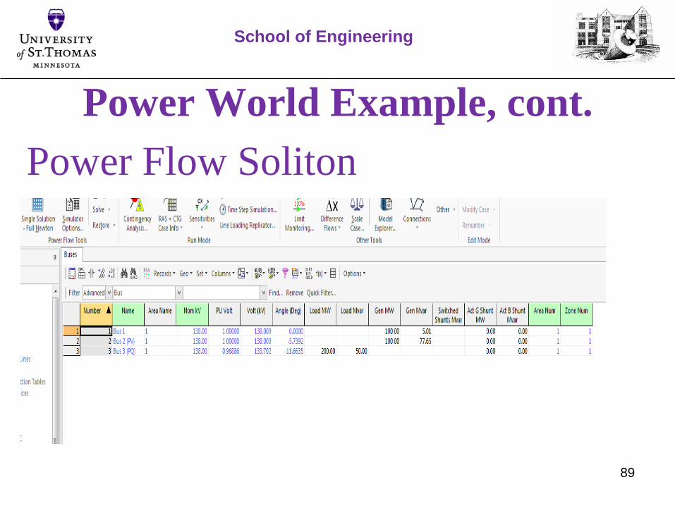
Bus No V 𝜹 P Q

One 1 0𝑜 1 0.05

Two 1 −5.7392𝑜 1 0.776

Three 0.9689 −11.664𝑜 −2 -0.5

86

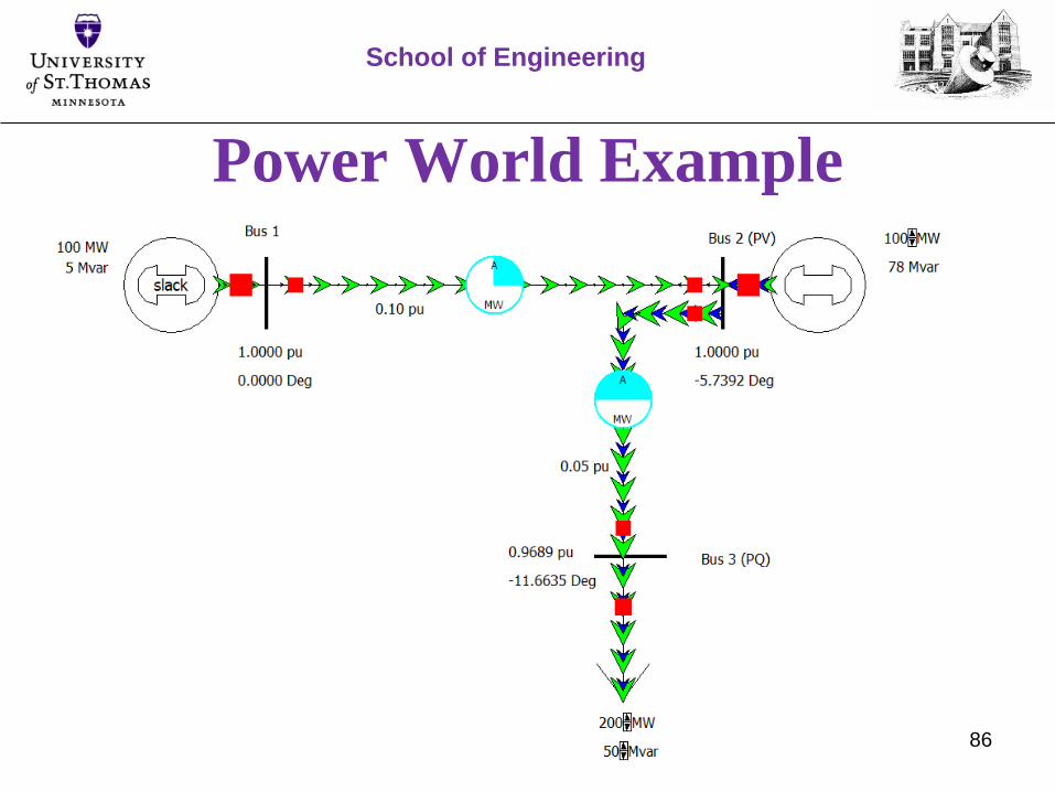
Power World Example


87

Power World Example, cont.


Y-Bus

88



Jacobin Matrix

89



Power Flow Soliton

Transmission Lines and Power Flow Analysis - UMN … Lines and Power Flow Analysis Dr. Greg Mowry...

Documents

Transcript of Transmission Lines and Power Flow Analysis - UMN … Lines and Power Flow Analysis Dr. Greg Mowry...