ClickHere

for

FullArticle

Transient luminous events above two mesoscale convectivesystems: Storm structure and evolution

Timothy J. Lang,1 Walter A. Lyons,2 Steven A. Rutledge,1 Jonathan D. Meyer,2,3

Donald R. MacGorman,4 and Steven A. Cummer5

Received 28 May 2009; revised 17 November 2009; accepted 4 December 2009; published 7 May 2010.

[1] Two warm‐season mesoscale convective systems (MCSs) were analyzed with respectto their production of transient luminous events (TLEs), mainly sprites. The 20 June 2007symmetric MCS produced 282 observed TLEs over a 4 h period, during which the storm’sintense convection weakened and its stratiform region strengthened. TLE productioncorresponded well to convective intensity. The convective elements of the MCS containednormal‐polarity tripole charge structures with upper‐level positive charge (<−40°C),midlevel negative charge (−20°C), and low‐level positive charge near the melting level.In contrast to previous sprite studies, the stratiform charge layer involved in TLEproduction by parent positive cloud‐to‐ground (+CG) lightning resided at upper levels.This layer was physically connected to upper‐level convective positive charge via adownward sloping pathway. The average altitude discharged by TLE‐parent flashes duringTLE activity was 8.2 km above mean sea level (MSL; −25°C). The 9 May 2007asymmetric MCS produced 25 observed TLEs over a 2 h period, during which the storm’sconvection rapidly weakened before recovering later. Unlike 20 June, TLE productionwas approximately anticorrelated with convective intensity. The 9 May storm, which alsohad a normal tripole in its convection, best fit the conventional model of low‐altitudepositive charge playing the dominant role in sprite production; however, the averagealtitude discharged during the TLE phase of flashes still was higher than the melting level:6.1 km MSL (−15°C). Based on these results, it is inferred that sprite production andsprite‐parent positive charge altitude depend on MCS morphology.

Citation: Lang, T. J., W. A. Lyons, S. A. Rutledge, J. D. Meyer, D. R. MacGorman, and S. A. Cummer (2010), Transientluminous events above two mesoscale convective systems: Storm structure and evolution, J. Geophys. Res., 115, A00E22,doi:10.1029/2009JA014500.

1. Introduction

[2] Sprites, a class of transient luminous event (TLE)that occurs above thunderstorms, are thought to result fromdielectric breakdown at approximately 75 km height [Stanleyet al., 1999]. Breakdown is induced by a strong transientelectric field resulting from the removal of large amountsof charge in a cloud‐to‐ground (CG) lightning flash [Paskoet al., 1996, 1997; Williams, 2001]. As initially suggestedby Wilson [1924], an important metric in this process is thecharge moment change (CMC):

�Mq tð Þ ¼ Zq tð Þ � Q tð Þ Ckmð Þ; ð1Þ

where Zq is the altitude (above ground level, AGL) fromwhich the charge Q is lowered to ground, both as functionsof time t. Various studies have suggested that for suchbreakdown to occur, total DMq values would need to beat least on the order of hundreds of C km [Bell et al., 1995;Pasko et al., 1997; Huang et al., 1999; Williams, 2001;Cummer and Lyons, 2005]. These values are extremely largecompared to typical CG strokes [Cummer and Lyons, 2004].[3] As reviewed by Williams and Yair [2006], in order to

achieve these large CMC values, the present paradigm forsprite production in warm‐season thunderstorms is the dis-charging of hundreds of C of positive charge within a lat-erally extensive layer near 0°C in the stratiform region of amesoscale convective system (MCS) [Houze et al., 1990] byenergetic positive CG (+CG) lightning [Marshall and Rust,1993; Boccippio et al., 1995; Lyons, 1996; Marshall et al.,1996; Williams, 1998; Marshall et al., 2001; Williams,2001; Lyons et al., 2003]. Such lightning often propagatesalong cloud base and is called “spider lightning” [Marshallet al., 1989; Mazur et al., 1995, 1998].[4] However, balloon‐borne electric field meter measure-

ments have established that multiple positive charge layers

1Department of Atmospheric Science, Colorado State University, FortCollins, Colorado, USA.

2FMA Research, Inc., Fort Collins, Colorado, USA.3Now at Department of Atmospheric Sciences, South Dakota School of

Mines and Technology, Rapid City, South Dakota, USA.4National Severe Storms Laboratory, Norman, Oklahoma, USA.5Department of Electrical Engineering, Duke University, Durham,

North Carolina, USA.

Copyright 2010 by the American Geophysical Union.0148‐0227/10/2009JA014500

JOURNAL OF GEOPHYSICAL RESEARCH, VOL. 115, A00E22, doi:10.1029/2009JA014500, 2010

A00E22 1 of 22

can exist with the stratiform region of an MCS [Chauzy etal., 1985; Schuur et al., 1991; Marshall and Rust, 1993;Stolzenburg et al., 1994, 1998, 2001]. In addition, thenumber and altitudes of the positive charge layers appear todepend on MCS morphology, with differences seen betweenasymmetric and symmetric MCSs [Schuur and Rutledge,2000a], as well as between bow echo, “squall line,” andpredominantly stratiform MCSs [Marshall and Rust, 1993].[5] Indeed, in recent years three‐dimensional lightning

mapping studies have shown that stratiform lightning canpropagate in different positive layers. One of these is anupper‐level (<−20°C), often downward sloping layer [Careyet al., 2005; Dotzek et al., 2005; Steiger et al., 2007; Elyet al., 2008; Lang and Rutledge, 2008; MacGorman et al.,2008]. Another is a midlevel layer near −10 to −15°C [Langet al., 2004; Carey et al., 2005; Lang and Rutledge, 2008;MacGorman et al., 2008; Lu et al., 2009]. Finally, laterallyextensive positive charge near 0°C can be active in lightning[Carey et al., 2005; Lang and Rutledge, 2008], includingsprite‐parent lightning [Lyons et al., 2003]. It is this lastlayer that best fits the current paradigm for sprite‐parentlightning.[6] However, while the near‐0°C layer has been observed

to be involved in the initiation of stratiform lightning [Langand Rutledge, 2008], it is not always observed as the mostactive stratiform lightning pathway. For example, the sym-metric MCS studied by Carey et al. [2005] had the mostlightning occurring along the upper pathway, while theasymmetric MCS studied by Lang et al. [2004] and Lang andRutledge [2008] had the midlevel pathway as the most elec-trically active. Ely et al. [2008] inferred that the slope andaltitude of lightning‐active charge layers in the stratiformregion may depend on updraft‐influenced microphysicalprocesses there. In addition, energetic and likely sprite‐producing +CGs in MCSs studied by Marshall et al. [2001]and Lu et al. [2009] did not propagate at 0°C. Therefore, itis hypothesized that sprite‐parent +CG lightning can tapcharge layers other than one near 0°C. Additionally, thespecific layer that is discharged may depend on MCSmorphology.[7] While it is well known that the typical meteorological

scenario for sprites involves MCSs with both ongoingconvection and laterally extensive stratiform rain areas[Lyons, 2006], the relationships between sprite productionand convective intensity, the microphysical structure of thestratiform region, and MCS organizational structure remainuncertain. Lyons [1996] found little direct correlation be-tween CG rate and sprite production, as sprite productionpeaked ∼1 h later than the CG peak. Assuming CG rate is anapproximate measure of convective intensity in MCSs, thissuggests that sprite production is not directly correlated withconvective intensity. These results are supported by Lyons etal. [2003], who noted a significant descent in the altitude oflightning activity before sprite production began as low‐level discharges associated with the melting layer began todominate within the stratiform region.[8] However, such a result may depend critically on the

preferred initiation locations for sprite‐parent lightning.Lang et al. [2004] noted that stratiform +CG lightning caninitiate both within the convective line as well as within thestratiform region. If sprite parent lightning typically initiatesin the convective line, it is reasonable to expect that total

flash rate in this convection, a direct measure of its intensity[Williams et al., 1999], could modulate sprite production inan MCS. This would be particularly true if the lightningtraveled through the upper‐level charge layer, since thisappears to be fed via charge advection from the convectiveline [Rutledge and MacGorman, 1988; Stolzenburg et al.,1994, 2001; Carey et al., 2005].[9] If most sprite parents initiate within the stratiform

region, then sprite production may depend on in situ charg-ing there [Marshall and Rust, 1993; Rutledge and Petersen,1994; Stolzenburg et al., 1994; Shepherd et al., 1996], andthus would depend on significant microphysical develop-ment within the stratiform region, a process that occurs latein MCS lifecycles. This would match the observed behaviorof both stratiform‐initiated lightning [Lang et al., 2004;Lang and Rutledge, 2008], as well as sprite production ingeneral.[10] Both charge advection and in situ charging are

important in MCS stratiform regions [Stolzenburg et al.,1994; Schuur and Rutledge, 2000b], and these two pro-cesses may account for different charge layers [Shepherdet al., 1996; Carey et al., 2005; Lang and Rutledge, 2008]as well as different classes of stratiform +CG lightning[Rutledge et al., 1990]. Therefore, it is hypothesized that therelationships between sprite production and MCS intensityand structure may be complex, and may depend on thedominant sprite‐parent charge layer, and on the dominantphysical process (charge advection or in situ) that led to thecreation of that layer.[11] On 9 May and 20 June 2007, TLE‐producing MCSs

were observed over central Oklahoma. In this paper, thestructure and evolution of these two storms are examinedin detail, in order to investigate the scientific questions thathave been raised regarding MCS morphology, the dominantcharge altitude for sprite‐parent lightning, and the relation-ship between MCS intensity, structure, and sprite production.

2. Data and Methodology

2.1. Overview

[12] Figure 1 shows key components of the observing net-work for 9 May and 20 June storms, which occurred duringa field experiment informally titled Sprites 2007. The avail-able instrumentation included several radars, geostationarysatellite observations, forecast model output, video camerasto capture TLEs, a network of charge moment change sen-sors, a very high frequency (VHF) three‐dimensional (3‐D)lightning mapper, and a CG lightning detection network.Each component of the observing network will be discussedindividually. Data analysis focused on the 03–05 UTC timeperiod for 9 May and 03–07 UTC on 20 June, when TLEswere observed.

2.2. Radars

[13] Reflectivity data from the Weather Surveillance Radar88 Doppler (WSR‐88D) network were used to characterizethe structure and evolution of the MCSs. The 9 May stormwas relatively small, and data from a single radar at Okla-homa City, OK (KTLX), were used. The 20 June storm wasextremely large, and thus data from several radars weremerged to create a 3‐D mosaic. These radars includedKTLX; Vance Air Force Base, OK (KVNX); Tulsa, OK

LANG ET AL.: TLES ABOVE MESOSCALE CONVECTIVE SYSTEMS A00E22A00E22

2 of 22

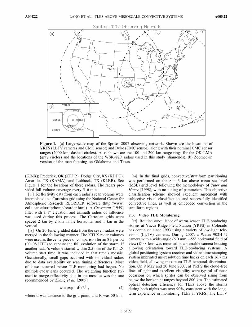
(KINX); Frederick, OK (KFDR); Dodge City, KS (KDDC);Amarillo, TX (KAMA); and Lubbock, TX (KLBB). SeeFigure 1 for the locations of these radars. The radars pro-vided full‐volume coverage every 5–6 min.[14] Reflectivity data from each radar’s scan volume were

interpolated to a Cartesian grid using the National Center forAtmospheric Research REORDER software (http://www.eol.ucar.edu/rdp/home/reorder.html). A Cressman [1959]filter with a 1° elevation and azimuth radius of influencewas used during this process. The Cartesian grids werespaced 2 km by 2 km in the horizontal and 1 km in thevertical.[15] On 20 June, gridded data from the seven radars were

merged in the following manner. The KTLX radar volumeswere used as the centerpiece of comparison for an 8 h period(00–08 UTC) to capture the full evolution of the storm. Ifanother radar’s volume started within 2.5 min of the KTLXvolume start time, it was included in that time’s mosaic.Occasionally, small gaps occurred with individual radarsdue to data availability or scan timing differences. Mostof these occurred before TLE monitoring had begun. Nomultiple‐radar gaps occurred. The weighting function (w)used to merge reflectivity data in the mosaics was the onerecommended by Zhang et al. [2005]:

w ¼ exp �d2=R2� �

; ð2Þwhere d was distance to the grid point, and R was 50 km.

[16] In the final grids, convective/stratiform partitioningwas performed on the z = 3 km above mean sea level(MSL) grid level following the methodology of Yuter andHouze [1998], with no tuning of parameters. This objectiveclassification scheme showed excellent agreement withsubjective visual classification, and successfully identifiedconvective lines, as well as embedded convection in thestratiform regions.

2.3. Video TLE Monitoring

[17] Routine surveillance of warm‐season TLE‐producingstorms at Yucca Ridge Field Station (YRFS) in Coloradohas continued since 1993 using a variety of low‐light tele-vision (LLTV) cameras. During 2007, a Watec 902H Ucamera with a wide‐angle (6.0 mm, ∼55° horizontal field ofview) f/0.8 lens was mounted in a steerable camera housingallowing orientation toward TLE‐producing systems. Aglobal positioning system receiver and video time‐stampingsystem imprinted ms‐resolution time hacks on each 16.7 msvideo field, allowing maximum TLE temporal discrimina-tion. On 9 May and 20 June 2007, at YRFS the cloud‐freelines of sight and excellent visibility were typical of thoseoccasions on which sprites can be observed rising frombelow the horizon at ranges beyond 800 km. The estimatedoptical detection efficiency for TLEs above the stormsduring both nights was over 90%, consistent with the long‐term experience in monitoring TLEs at YRFS. The LLTV

Figure 1. (a) Large‐scale map of the Sprites 2007 observing network. Shown are the locations ofYRFS (LLTV cameras and CMC sensor) and Duke (CMC sensor), along with their nominal CMC sensorranges (2000 km; dashed circles). Also shown are the 100 and 200 km range rings for the OK‐LMA(gray circles) and the locations of the WSR‐88D radars used in this study (diamonds). (b) Zoomed‐inversion of the map focusing on Oklahoma and Texas.

LANG ET AL.: TLES ABOVE MESOSCALE CONVECTIVE SYSTEMS A00E22A00E22

3 of 22

field of view was sufficiently wide to encompass all of theMCSs on both dates.

2.4. National Lightning Detection Network

[18] National Lightning Detection Network (NLDN) stroke‐level data were used in this study. The NLDN can misclas-sify intracloud (IC) flashes as +CGs, and so +CGs with peakcurrents under 10 kA were not considered [Cummins et al.,1998]. Parent CGs were matched to observed TLEs via themethodology of Lyons et al. [2003, 2008], which comparedTLE timing and azimuth to NLDN strike timing and location.Not all TLE‐parent +CGs were detected by the NLDN. Only230 of 282 observed TLEs on 20 June had a detected +CGparent (82%), while 23 of 25 observed TLEs on 9 May werematched to a detected parent +CG (92%). Therefore, theanalysis in this study was confined to only TLEs with adetected parent +CG flash. This does not imply that someTLEs were IC‐produced, as NLDN detection efficiency isbelow 100% and TLE parent CGs may have complex waveforms (K. Cummins, personal communication, 2009).

2.5. Charge Moment Change Network

[19] A prototype Charge Moment Change Network(CMCN) with essentially national coverage (Figure 1) wasestablished by placing two highly sensitive broadband mag-netic sensors (ultralow through very low frequency, <1 Hzto 30 kHz) at YRFS and Durham, NC (Duke University).The details of this system are discussed by Lyons et al.[2009]. Real‐time processing retrieved the impulse chargemoment change (iDMq), which is the charge moment changecontributed within the first ∼2 ms of the CG discharge[Cummer and Lyons, 2005]. These time‐tagged iDMq eventswere geolocated via temporal matching with NLDN CGsof the appropriate polarity. Web‐based displays, updatedevery 5 min, allowed identifying storms generating potentialsprite‐parent CGs, typically positive iDMq events >100 Ckm, with more than 60–80% producing optically confirmedTLEs when values were >300 C km. While real‐time datawere utilized in the detection of TLEs (e.g., the CMCNdisplay was very valuable in orienting the camera towardTLE‐producing regions), detailed analysis of the CMC datawill appear in a subsequent paper.

2.6. Three‐Dimensional VHF Lightning MappingArray

2.6.1. Overview[20] The Oklahoma Lightning Mapping Array (OK‐LMA)

is a time‐of‐arrival 3‐D lightning mapping system developedby the New Mexico Institute of Mining and Technology(NMIMT), and operated by the University of Oklahoma,the National Severe Storms Laboratory, and NMIMT[MacGorman et al., 2008]. The OK‐LMA maps lightningby receiving radiation produced in a specific VHF bandas a flash develops. Flashes commonly consist of tens tothousands of individual VHF sources. The design, opera-tion, and accuracy of LMAs has been discussed extensivelyby Rison et al. [1999], Krehbiel et al. [2000], and Thomas etal. [2004], and this section will focus only on details rele-vant to the present study.[21] Only VHF sources detected by at least 7 stations were

examined, and goodness‐of‐fit values (c2) were required

to be ≤ 1.0 in the source location solutions. These criteriaallowed excellent 3‐D visualization of flashes while mini-mizing the influence of noisy or poorly located sources,similar to the methodology of Lang and Rutledge [2008].[22] MacGorman et al. [2008] noted that the 3‐D map-

ping of lightning flashes by the OK‐LMA is optimal within100 km of the network center, while two‐dimensional (2‐D)mapping is optimal within 200 km range. The presentstudy considered a massive MCS that spanned two states(20 June). Notably, only a portion of the 20 June storm waswithin 200 km of the OK‐LMA center at any one time.Therefore, the total lightning mapping of the 20 June stormwas limited. Moreover, most TLE‐parent lightning coveredlarge horizontal distances (∼100 km or more in the largestdimension). Therefore, the mapping quality of individualTLE‐producing flashes varied depending on the particularflash or flash section being examined. The resolution of theOK‐LMA, and its impact on this study’s results, are treatedin more detail in Appendix A.2.6.2. Flash Analysis[23] TLE‐parent flashes were manually identified and

isolated using NMIMT’s XLMA lightning viewing soft-ware. The source data associated with each flash (i.e.,time, altitude, latitude‐longitude coordinates) were saved forlater analysis with in‐house Interactive Data Language(IDL) programs. For 20 June, TLE‐producing flashes withdetected parent +CGs within 175 km of the LMA centerwere analyzed (49 total TLE‐producing +CGs). For 9 May,the furthest TLE‐parent +CG was 93 km, and so all detectedTLE parents were analyzed (23 total).[24] Various parameters were computed for each flash.

Initiation height (ZINIT) was taken from the mean locationof the first 10 sources. Initiation reflectivity was obtainedfrom the radar grid point containing this location, and CGreflectivity was taken from the near‐surface reflectivity atthe strike grid point. Time to CG was the time betweenflash initiation (in the VHF data) to CG strike time. Flasharea was the area of the smallest rectangle containing allVHF sources in a flash. Height of the flash during theTLE (ZTLE) was the mean of all sources after the parent+CG through the end of the TLE time. This was essen-tially an estimate of Zq in equation (1) [Lyons et al., 2003].To ensure nearly normal statistics, a minimum of 30 sourceswere required to compute ZTLE [Walpole et al., 2002]. Iffewer sources were available (which happened for 13 totalTLEs), the time period was extended until 30 sources wereobtained. If the end of the flash was reached beforehand(which happened with one TLE), then the difference wasmade up with sources immediately prior to the parent CG.For context, the average number of sources contributing toZTLE on 20 June was 250 (the mean for 9 May was 440).This methodology was similar to that used by Lyons et al.[2003, 2008] for calculating Zq.[25] Some 20 June LMA‐mapped flashes produced more

than one TLE‐parent +CG. In these circumstances, twoseparate estimates for unique parameters such as ZTLE werekept, while duplicate parameters such as ZINIT were countedonly once.2.6.3. Charge Identification[26] Manual charge identification using the LMA data

was performed following Rison et al. [1999], Rust et al.

LANG ET AL.: TLES ABOVE MESOSCALE CONVECTIVE SYSTEMS A00E22A00E22

4 of 22

[2005], and Wiens et al. [2005]. This technique assumedthe bidirectional electric field breakdown model for light-ning discharges proposed by Kasemir [1960] and furtheradvocated by Mazur and Ruhnke [1993]. It was based onthe fact that negative breakdown through positive chargelayers is inherently more noisy at VHF than positivebreakdown though negative charge, leading to more VHFsources being detected in positive charge layers than innegative [Rison et al., 1999]. The technique usually assignedcharge for a flash within a charge dipole based on theinitial vertical direction of the negative leader discharge. Ifupward, then the dipole was assumed to be positive chargeover negative charge; if downward, the opposite. Relativedistribution of VHF sources with altitude also was used tohelp identify charge layers. This technique shows goodagreement with charge distributions inferred from balloon‐borne electric field soundings [Coleman et al., 2003; Rust etal., 2005; MacGorman et al., 2008], and it has been suc-cessfully applied by other researchers [Wiens et al., 2005;Lang and Rutledge, 2008] to infer physically reasonablegross charge distributions in thunderstorms. Due to thelarge number of flashes in this MCS, charge was sortedonly for select flashes.[27] When manual sorting was not feasible, charge iden-

tification was done by examination of VHF source densitymaps for LMA‐visible portions of the MCS during specifictime periods. This methodology was based on the afore-mentioned results of Rison et al. [1999] and has been usedto infer physically reasonable charge distributions by Careyet al. [2005]. Regions of maximum source density typicallywere attributed to the presence of positive charge. However,this was not always the case, and hand analysis of selectflashes was used to confirm all inferences.[28] LMA‐based charge identification is limited by the

fact that only charge involved in lightning can be mapped.In addition, charge does not always exist in regions whereLMA sources propagate (particularly when LMA sourcesexist in gaps between charge layers, e.g., the initiationlocation of an IC flash). Finally, care needs to be taken ininterpreting data containing large numbers of flashes, due tohorizontal heterogeneity in charge structure or the presenceof thin, vertically stacked layers of opposite charge.

2.7. Other Data

[29] Large, warm‐season MCSs over the U.S. High Plainsappear to be among the most efficient at generating light-ning discharges meeting the requirements for sprites, halos,and elves [Lyons, 2006]. Fifteen years of monitoring andforecasting experience has demonstrated that TLEs areincreasingly likely when the −50°C cloud area associatedwith an MCS exceeds 25,000 km2, with the coldest topsoften −60°C or less. The MCS also must possess a largeregion of stratiform precipitation (>10–20 × 103 km2), anda smaller, intense convective core with peak reflectivities>55 dBZ [Lyons, 2006; Lyons et al., 2006]. Therefore, real‐time weather data, such as infrared brightness temperaturedata from the Geostationary Operational EnvironmentalSatellite (GOES) network, routine output from the RapidUpdate Cycle (RUC) weather forecast model [Benjamin etal., 2004a, 2004b], and national mosaics of WSR‐88Dreflectivity, were used to identify and characterize TLE‐

producing storms. In addition, 00 UTC Oklahoma Citysounding data on 9 May and 20 June were used to char-acterize temperature levels.

3. Results

3.1. Overview of Cases

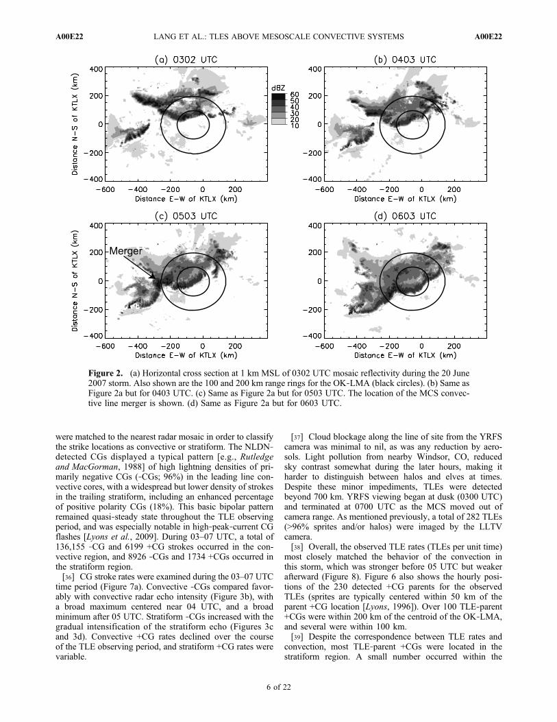
3.1.1. The 20 June 2007 Case[30] The meteorological context for this case has been

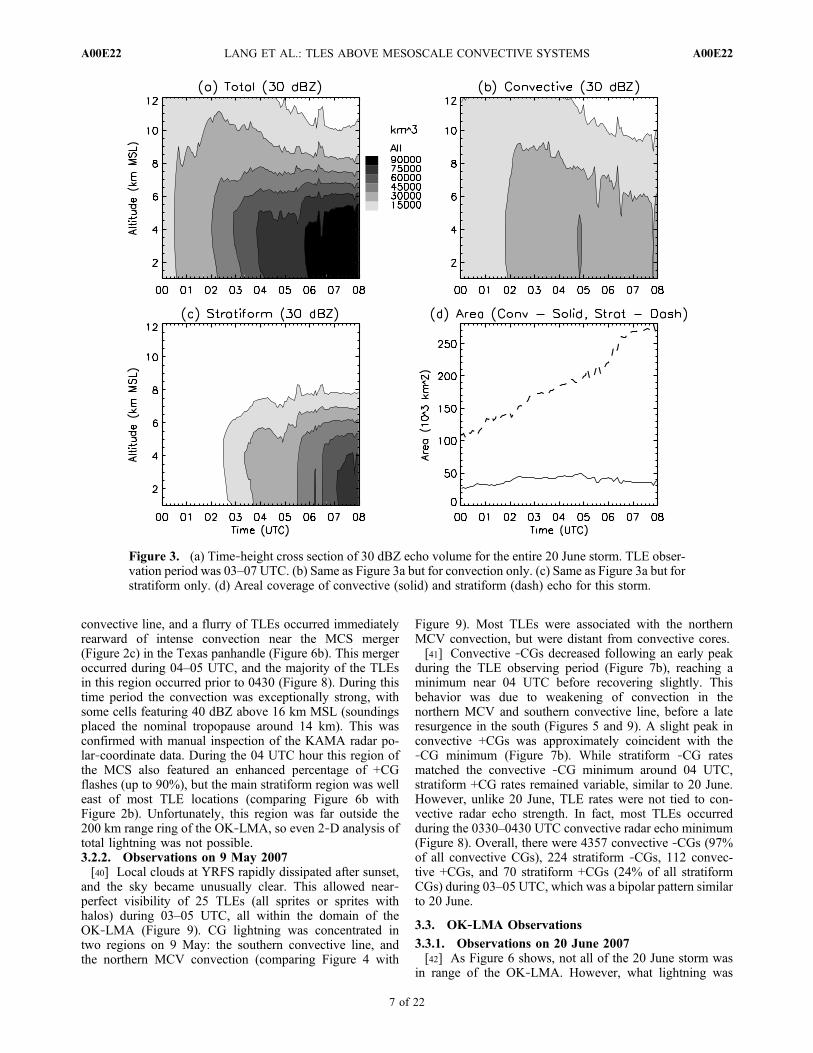
discussed previously by Lyons et al. [2009]. The basicstructure of the storm, which experienced a merger betweentwo separate MCSs during its lifetime, defined it as asymmetric leading‐line/trailing stratiform MCS (Figure 2)[Houze et al., 1990]. It was partially contained within theOK‐LMA domain during much of the TLE observing period(03–07 UTC). Though not discussed in detail here, theMCS qualified as a mesoscale convective complex (MCC)[Maddox, 1980], and was perhaps the largest MCC of theseason in the central U.S.[31] Horizontal and vertical evolution of radar echoes in

the convective and stratiform regions of the MCS wereexamined in more detail (Figure 3). The TLE observingperiod was characterized by intense but gradually weaken-ing convection, while the stratiform region was intensifying,a classic pattern in MCSs [Houze et al., 1990]. Stratiformarea more than doubled over the analysis period, whileconvective area stayed nearly constant.3.1.2. The 9 May 2007 Case[32] On 9 May 2007, a persistent upper‐level trough

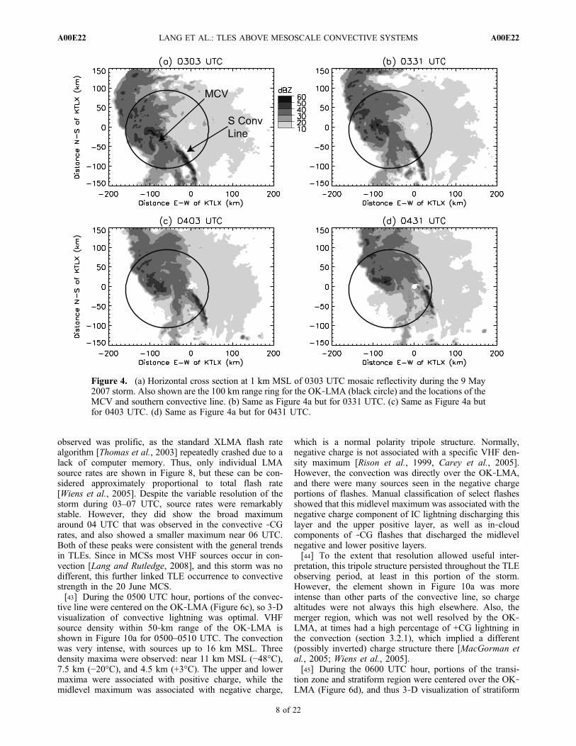
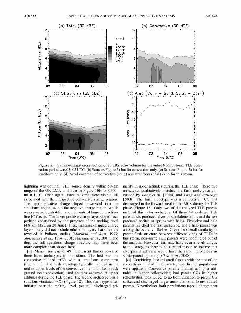
over the Rockies sent a wave of storms into western Texas,which evolved upscale into MCSs while moving northeastinto Oklahoma. GOES and KTLX radar imagery showedthat a large storm system was centered over the OK‐LMAby 03 UTC (Figure 4). The −50°C cloud canopy area(61,000 km2) during 04–05 UTC exceeded sprite criteria, asdid peak convective radar reflectivity and stratiform radarecho area (Figure 5).[33] The structure of this storm (Figure 4) classified it

as an asymmetric MCS [Houze et al., 1990], consisting ofa convective line to the southeast, with a stratiform regionto the northwest. Radar imagery loops showed that thenorthern stratiform region was rotating cyclonically as amesoscale convective vortex (MCV) [Smull and Houze,1985; Scott and Rutledge, 1995; Davis et al., 2004]. TheMCV also contained disorganized embedded convection(Figure 4), which was the remnant of the northern portionof the original convective line that was wrapped up by theMCV prior to 03 UTC.[34] By 05 UTC, RUC‐estimated CAPE in the region rap-

idly depleted to values below 1500 J kg−1. After 0430 UTC,cloud tops began to subside, and TLE production endedshortly after 05 UTC. During much of the TLE observingperiod (03–05 UTC), the vertical radar structure of the stormgradually weakened, although areal coverage remained rel-atively stable (Figure 5). However, despite the subsidingcloud tops, there was an increase in convective intensityafter 0430 UTC (Figure 5b).

3.2. CG and TLE Observations

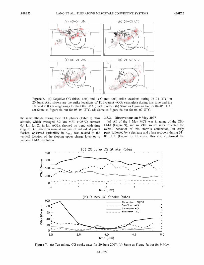
3.2.1. Observations on 20 June 2007[35] The hourly evolution of CG and TLE‐parent CG

strike locations on 20 June is shown in Figure 6. CG strikes

LANG ET AL.: TLES ABOVE MESOSCALE CONVECTIVE SYSTEMS A00E22A00E22

5 of 22

were matched to the nearest radar mosaic in order to classifythe strike locations as convective or stratiform. The NLDN‐detected CGs displayed a typical pattern [e.g., Rutledgeand MacGorman, 1988] of high lightning densities of pri-marily negative CGs (‐CGs; 96%) in the leading line con-vective cores, with a widespread but lower density of strokesin the trailing stratiform, including an enhanced percentageof positive polarity CGs (18%). This basic bipolar patternremained quasi‐steady state throughout the TLE observingperiod, and was especially notable in high‐peak‐current CGflashes [Lyons et al., 2009]. During 03–07 UTC, a total of136,155 ‐CG and 6199 +CG strokes occurred in the con-vective region, and 8926 ‐CGs and 1734 +CGs occurred inthe stratiform region.[36] CG stroke rates were examined during the 03–07 UTC

time period (Figure 7a). Convective ‐CGs compared favor-ably with convective radar echo intensity (Figure 3b), witha broad maximum centered near 04 UTC, and a broadminimum after 05 UTC. Stratiform ‐CGs increased with thegradual intensification of the stratiform echo (Figures 3cand 3d). Convective +CG rates declined over the courseof the TLE observing period, and stratiform +CG rates werevariable.

[37] Cloud blockage along the line of site from the YRFScamera was minimal to nil, as was any reduction by aero-sols. Light pollution from nearby Windsor, CO, reducedsky contrast somewhat during the later hours, making itharder to distinguish between halos and elves at times.Despite these minor impediments, TLEs were detectedbeyond 700 km. YRFS viewing began at dusk (0300 UTC)and terminated at 0700 UTC as the MCS moved out ofcamera range. As mentioned previously, a total of 282 TLEs(>96% sprites and/or halos) were imaged by the LLTVcamera.[38] Overall, the observed TLE rates (TLEs per unit time)

most closely matched the behavior of the convection inthis storm, which was stronger before 05 UTC but weakerafterward (Figure 8). Figure 6 also shows the hourly posi-tions of the 230 detected +CG parents for the observedTLEs (sprites are typically centered within 50 km of theparent +CG location [Lyons, 1996]). Over 100 TLE‐parent+CGs were within 200 km of the centroid of the OK‐LMA,and several were within 100 km.[39] Despite the correspondence between TLE rates and

convection, most TLE‐parent +CGs were located in thestratiform region. A small number occurred within the

Figure 2. (a) Horizontal cross section at 1 km MSL of 0302 UTC mosaic reflectivity during the 20 June2007 storm. Also shown are the 100 and 200 km range rings for the OK‐LMA (black circles). (b) Same asFigure 2a but for 0403 UTC. (c) Same as Figure 2a but for 0503 UTC. The location of the MCS convec-tive line merger is shown. (d) Same as Figure 2a but for 0603 UTC.

LANG ET AL.: TLES ABOVE MESOSCALE CONVECTIVE SYSTEMS A00E22A00E22

6 of 22

convective line, and a flurry of TLEs occurred immediatelyrearward of intense convection near the MCS merger(Figure 2c) in the Texas panhandle (Figure 6b). This mergeroccurred during 04–05 UTC, and the majority of the TLEsin this region occurred prior to 0430 (Figure 8). During thistime period the convection was exceptionally strong, withsome cells featuring 40 dBZ above 16 km MSL (soundingsplaced the nominal tropopause around 14 km). This wasconfirmed with manual inspection of the KAMA radar po-lar‐coordinate data. During the 04 UTC hour this region ofthe MCS also featured an enhanced percentage of +CGflashes (up to 90%), but the main stratiform region was welleast of most TLE locations (comparing Figure 6b withFigure 2b). Unfortunately, this region was far outside the200 km range ring of the OK‐LMA, so even 2‐D analysis oftotal lightning was not possible.3.2.2. Observations on 9 May 2007[40] Local clouds at YRFS rapidly dissipated after sunset,

and the sky became unusually clear. This allowed near‐perfect visibility of 25 TLEs (all sprites or sprites withhalos) during 03–05 UTC, all within the domain of theOK‐LMA (Figure 9). CG lightning was concentrated intwo regions on 9 May: the southern convective line, andthe northern MCV convection (comparing Figure 4 with

Figure 9). Most TLEs were associated with the northernMCV convection, but were distant from convective cores.[41] Convective ‐CGs decreased following an early peak

during the TLE observing period (Figure 7b), reaching aminimum near 04 UTC before recovering slightly. Thisbehavior was due to weakening of convection in thenorthern MCV and southern convective line, before a lateresurgence in the south (Figures 5 and 9). A slight peak inconvective +CGs was approximately coincident with the‐CG minimum (Figure 7b). While stratiform ‐CG ratesmatched the convective ‐CG minimum around 04 UTC,stratiform +CG rates remained variable, similar to 20 June.However, unlike 20 June, TLE rates were not tied to con-vective radar echo strength. In fact, most TLEs occurredduring the 0330–0430 UTC convective radar echo minimum(Figure 8). Overall, there were 4357 convective ‐CGs (97%of all convective CGs), 224 stratiform ‐CGs, 112 convec-tive +CGs, and 70 stratiform +CGs (24% of all stratiformCGs) during 03–05 UTC, which was a bipolar pattern similarto 20 June.

3.3. OK‐LMA Observations

3.3.1. Observations on 20 June 2007[42] As Figure 6 shows, not all of the 20 June storm was

in range of the OK‐LMA. However, what lightning was

Figure 3. (a) Time‐height cross section of 30 dBZ echo volume for the entire 20 June storm. TLE obser-vation period was 03–07 UTC. (b) Same as Figure 3a but for convection only. (c) Same as Figure 3a but forstratiform only. (d) Areal coverage of convective (solid) and stratiform (dash) echo for this storm.

LANG ET AL.: TLES ABOVE MESOSCALE CONVECTIVE SYSTEMS A00E22A00E22

7 of 22

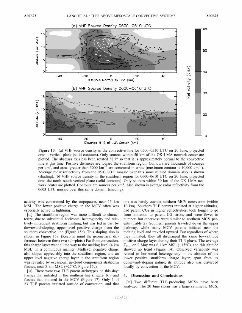
observed was prolific, as the standard XLMA flash ratealgorithm [Thomas et al., 2003] repeatedly crashed due to alack of computer memory. Thus, only individual LMAsource rates are shown in Figure 8, but these can be con-sidered approximately proportional to total flash rate[Wiens et al., 2005]. Despite the variable resolution of thestorm during 03–07 UTC, source rates were remarkablystable. However, they did show the broad maximumaround 04 UTC that was observed in the convective ‐CGrates, and also showed a smaller maximum near 06 UTC.Both of these peaks were consistent with the general trendsin TLEs. Since in MCSs most VHF sources occur in con-vection [Lang and Rutledge, 2008], and this storm was nodifferent, this further linked TLE occurrence to convectivestrength in the 20 June MCS.[43] During the 0500 UTC hour, portions of the convec-

tive line were centered on the OK‐LMA (Figure 6c), so 3‐Dvisualization of convective lightning was optimal. VHFsource density within 50‐km range of the OK‐LMA isshown in Figure 10a for 0500–0510 UTC. The convectionwas very intense, with sources up to 16 km MSL. Threedensity maxima were observed: near 11 km MSL (−48°C),7.5 km (−20°C), and 4.5 km (+3°C). The upper and lowermaxima were associated with positive charge, while themidlevel maximum was associated with negative charge,

which is a normal polarity tripole structure. Normally,negative charge is not associated with a specific VHF den-sity maximum [Rison et al., 1999, Carey et al., 2005].However, the convection was directly over the OK‐LMA,and there were many sources seen in the negative chargeportions of flashes. Manual classification of select flashesshowed that this midlevel maximum was associated with thenegative charge component of IC lightning discharging thislayer and the upper positive layer, as well as in‐cloudcomponents of ‐CG flashes that discharged the midlevelnegative and lower positive layers.[44] To the extent that resolution allowed useful inter-

pretation, this tripole structure persisted throughout the TLEobserving period, at least in this portion of the storm.However, the element shown in Figure 10a was moreintense than other parts of the convective line, so chargealtitudes were not always this high elsewhere. Also, themerger region, which was not well resolved by the OK‐LMA, at times had a high percentage of +CG lightning inthe convection (section 3.2.1), which implied a different(possibly inverted) charge structure there [MacGorman etal., 2005; Wiens et al., 2005].[45] During the 0600 UTC hour, portions of the transi-

tion zone and stratiform region were centered over the OK‐LMA (Figure 6d), and thus 3‐D visualization of stratiform

Figure 4. (a) Horizontal cross section at 1 km MSL of 0303 UTC mosaic reflectivity during the 9 May2007 storm. Also shown are the 100 km range ring for the OK‐LMA (black circle) and the locations of theMCV and southern convective line. (b) Same as Figure 4a but for 0331 UTC. (c) Same as Figure 4a butfor 0403 UTC. (d) Same as Figure 4a but for 0431 UTC.

LANG ET AL.: TLES ABOVE MESOSCALE CONVECTIVE SYSTEMS A00E22A00E22

8 of 22

lightning was optimal. VHF source density within 50‐kmrange of the OK‐LMA is shown in Figure 10b for 0600–0610 UTC. Once again, three maxima were visible, allassociated with their respective convective charge regions.The upper positive charge sloped downward into thestratiform region, as did the negative charge region, whichwas revealed by stratiform components of large convective‐line IC flashes. The lower positive charge layer sloped less,perhaps constrained by the presence of the melting level(4.8 km MSL on 20 June). These lightning‐mapped chargelayers likely did not include other thin layers that often arerevealed in balloon studies [Marshall and Rust, 1993;Stolzenburg et al., 1994, 2001; Marshall et al., 2001], andthus the full stratiform charge structure may have beenmore complex than shown here.[46] Manual analysis of 49 TLE‐parent flashes revealed

three basic archetypes in this storm. The first was theconvective‐initiated +CG with a stratiform component(Figure 11). This flash archetype typically initiated in themid to upper levels of the convective line (and often struckground near convection), and sources occurred at upperaltitudes during the TLE phase. The second archetype was astratiform‐initiated +CG (Figure 12). This flash type ofteninitiated near the melting level, yet still discharged pri-

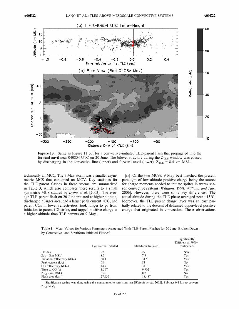
marily in upper altitudes during the TLE phase. These twoarchetypes qualitatively matched the flash archetypes dis-cussed by Lang et al. [2004] and Lang and Rutledge[2008]. The final archetype was a convective +CG thatdischarged in the forward anvil of the MCS during the TLEphase (Figure 13). Only two of the analyzed TLE parentsmatched this latter archetype. Of these 49 analyzed TLEparents, six produced elves or standalone halos, and the restproduced sprites or sprites with halos. Five elve and haloparents matched the first archetype, and a halo parent wasamong the two anvil flashes. Given the overall similarity inparent‐flash structure between different kinds of TLEs inthis storm, non‐sprite TLE parents were not filtered out ofthe analysis. However, this may have been a result uniqueto this study, as there is no a priori reason to assume thatelve‐parent lightning would have the same morphology assprite‐parent lightning [Chen et al., 2008].[47] Combining forward‐anvil flashes with the rest of the

convective‐initiated TLE parents, two distinct populationswere apparent. Convective parents initiated at higher alti-tudes in higher reflectivities, had parent CGs in higherreflectivities, took longer to go from initiation to parent CGstrike, and discharged larger areas than stratiform‐initiatedparents. Nevertheless, both populations tapped charge near

Figure 5. (a) Time‐height cross section of 30 dBZ echo volume for the entire 9 May storm. TLE obser-vation period was 03–05 UTC. (b) Same as Figure 5a but for convection only. (c) Same as Figure 5a but forstratiform only. (d) Areal coverage of convective (solid) and stratiform (dash) echo for this storm.

LANG ET AL.: TLES ABOVE MESOSCALE CONVECTIVE SYSTEMS A00E22A00E22

9 of 22

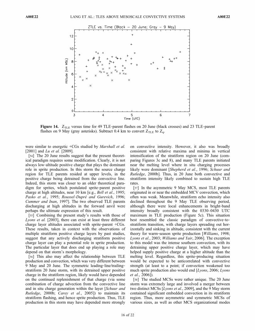
the same altitude during their TLE phases (Table 1). Thisaltitude, which averaged 8.2 km MSL (−25°C; subtract0.4 km for Zq in km AGL), showed no trend with time(Figure 14). Based on manual analysis of individual parentflashes, observed variability in ZTLE was related to thevertical location of the sloping upper charge layer or tovariable LMA resolution.

3.3.2. Observations on 9 May 2007[48] All of the 9 May MCS was in range of the OK‐

LMA (Figure 9), and so VHF source rates reflected theoverall behavior of this storm’s convection: an earlypeak followed by a decrease and a late recovery during 03–05 UTC (Figure 8). However, this also confirmed the

Figure 6. (a) Negative CG (black dots) and +CG (red dots) strike locations during 03–04 UTC on20 June. Also shown are the strike locations of TLE‐parent +CGs (triangles) during this time and the100 and 200 km range rings for the OK‐LMA (black circles). (b) Same as Figure 6a but for 04–05 UTC.(c) Same as Figure 6a but for 05–06 UTC. (d) Same as Figure 6a but for 06–07 UTC.

Figure 7. (a) Ten minute CG stroke rates for 20 June 2007. (b) Same as Figure 7a but for 9 May.

LANG ET AL.: TLES ABOVE MESOSCALE CONVECTIVE SYSTEMS A00E22A00E22

10 of 22

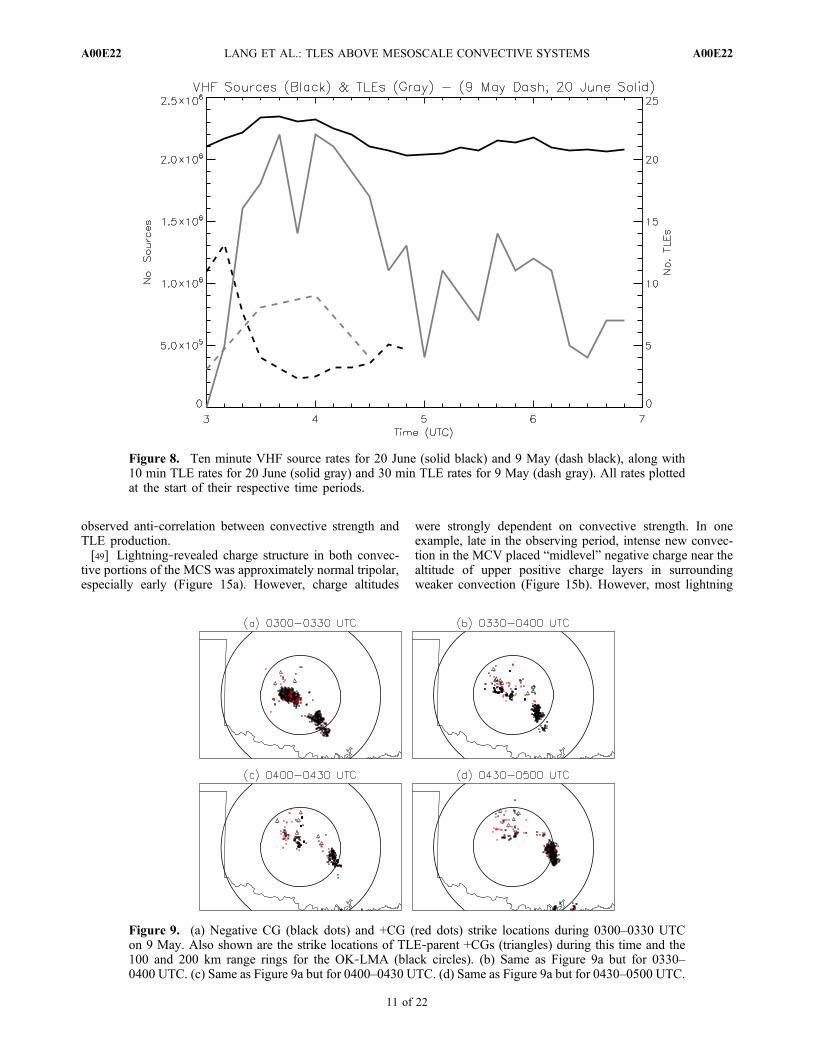
observed anti‐correlation between convective strength andTLE production.[49] Lightning‐revealed charge structure in both convec-

tive portions of the MCS was approximately normal tripolar,especially early (Figure 15a). However, charge altitudes

were strongly dependent on convective strength. In oneexample, late in the observing period, intense new convec-tion in the MCV placed “midlevel” negative charge near thealtitude of upper positive charge layers in surroundingweaker convection (Figure 15b). However, most lightning

Figure 8. Ten minute VHF source rates for 20 June (solid black) and 9 May (dash black), along with10 min TLE rates for 20 June (solid gray) and 30 min TLE rates for 9 May (dash gray). All rates plottedat the start of their respective time periods.

Figure 9. (a) Negative CG (black dots) and +CG (red dots) strike locations during 0300–0330 UTCon 9 May. Also shown are the strike locations of TLE‐parent +CGs (triangles) during this time and the100 and 200 km range rings for the OK‐LMA (black circles). (b) Same as Figure 9a but for 0330–0400 UTC. (c) Same as Figure 9a but for 0400–0430 UTC. (d) Same as Figure 9a but for 0430–0500 UTC.

LANG ET AL.: TLES ABOVE MESOSCALE CONVECTIVE SYSTEMS A00E22A00E22

11 of 22

activity was constrained by the tropopause, near 13 kmMSL. The lower positive charge in the MCV often wasespecially active in lightning.[50] The stratiform region was more difficult to charac-

terize, due to substantial horizontal heterogeneity and rela-tively infrequent stratiform flashing, but was fed in part bydownward‐sloping, upper‐level positive charge from thesouthern convective line (Figure 15c). This sloping also isshown in Figure 15a. (Keep in mind the geometrical dif-ferences between these two sub‐plots.) Far from convection,this charge layer went all the way to the melting level (4 kmMSL) in a continuous manner. Midlevel negative chargealso sloped appreciably into the stratiform region, and anupper‐level negative charge layer in the stratiform regionwas revealed by occasional in‐cloud components stratiformflashes, near 8 km MSL (−27°C; Figure 15c).[51] There were two TLE parent archetypes on this day:

flashes that initiated in the southern line (Figure 16), andflashes that initiated in the MCV (Figure 17). Only 1 of23 TLE parents initiated outside of convection, and that

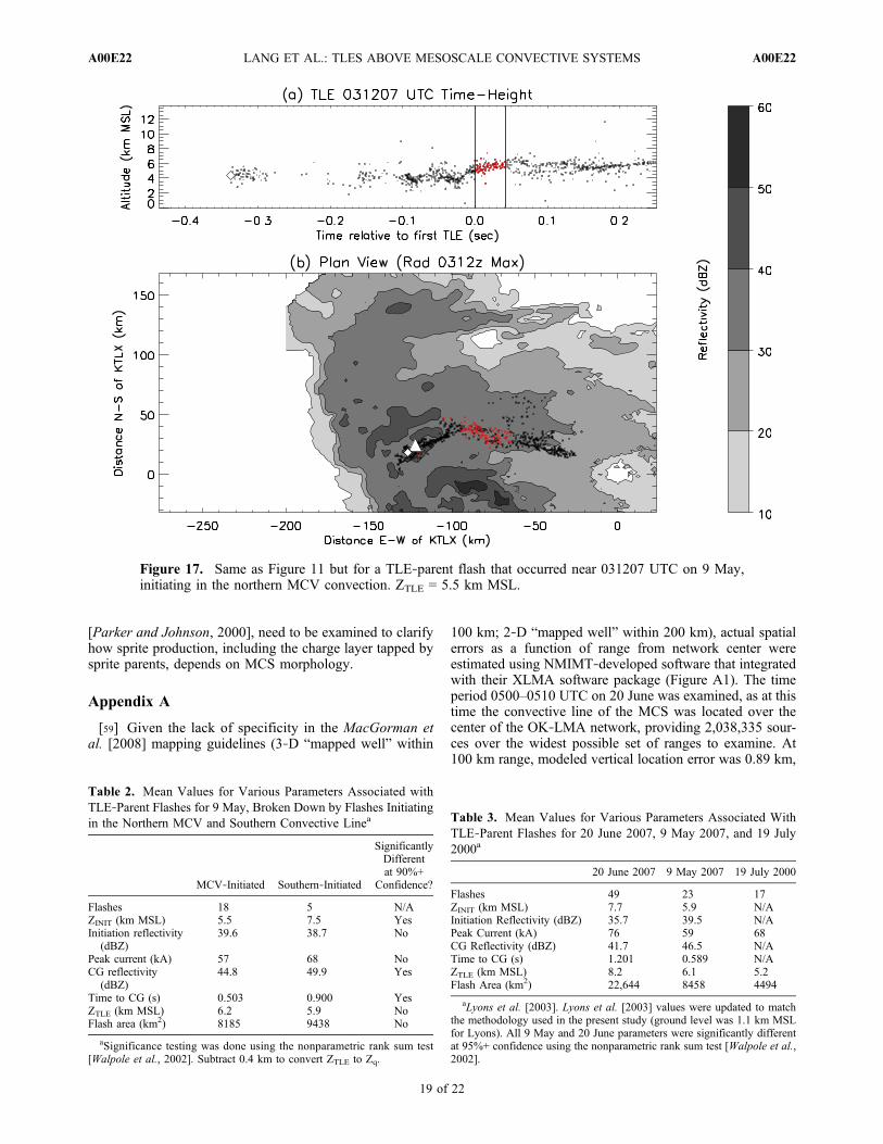
one was barely outside northern MCV convection (within10 km). Southern TLE parents initiated at higher altitudes,had parent CGs in higher reflectivities, took longer to gofrom initiation to parent CG strike, and were fewer innumber, but otherwise were similar to northern MCV par-ents (Table 2). Southern parents traveled down the upperpathway, while many MCV parents initiated near themelting level and traveled upward. But regardless of wherethey initiated, they all discharged the same low‐altitudepositive charge layer during their TLE phase. The averageZTLE on 9 May was 6.1 km MSL (−15°C), and this altitudeshowed no trend (Figure 14). Observed variability wasrelated to horizontal heterogeneity in the altitude of thelower positive stratiform charge layer; apart from itsdownward‐sloping nature, its altitude also was disturbedlocally by convection in the MCV.

4. Discussion and Conclusions

[52] Two different TLE‐producing MCSs have beenanalyzed. The 20 June storm was a large symmetric MCS,

Figure 10. (a) VHF source density in the convective line for 0500–0510 UTC on 20 June, projectedonto a vertical plane (solid contours). Only sources within 50 km of the OK‐LMA network center areplotted. The abscissa axis has been rotated 38.7° so that it is approximately normal to the convectiveline at this time. Positive distances are toward the stratiform region. Contours are thousands of sourcesper km2, and areas greater than 5000 km−2 are contoured in white (maximum contour is 10,000 km−2).Average radar reflectivity from the 0503 UTC mosaic over this same rotated domain also is shown(shading). (b) VHF source density in the stratiform region for 0600–0610 UTC on 20 June, projectedonto the north–south vertical plane (solid contours). Only sources within 50 km of the OK‐LMA net-work center are plotted. Contours are sources per km2. Also shown is average radar reflectivity from the0603 UTC mosaic over this same domain (shading).

LANG ET AL.: TLES ABOVE MESOSCALE CONVECTIVE SYSTEMS A00E22A00E22

12 of 22

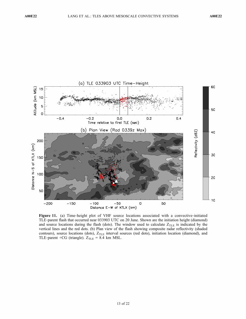
Figure 11. (a) Time‐height plot of VHF source locations associated with a convective‐initiatedTLE‐parent flash that occurred near 033903 UTC on 20 June. Shown are the initiation height (diamond)and source locations during the flash (dots). The window used to calculate ZTLE is indicated by thevertical lines and the red dots. (b) Plan view of the flash showing composite radar reflectivity (shadedcontours), source locations (dots), ZTLE interval sources (red dots), initiation location (diamond), andTLE‐parent +CG (triangle). ZTLE = 8.4 km MSL.

LANG ET AL.: TLES ABOVE MESOSCALE CONVECTIVE SYSTEMS A00E22A00E22

13 of 22

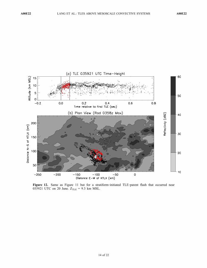
Figure 12. Same as Figure 11 but for a stratiform‐initiated TLE‐parent flash that occurred near035921 UTC on 20 June. ZTLE = 9.3 km MSL.

LANG ET AL.: TLES ABOVE MESOSCALE CONVECTIVE SYSTEMS A00E22A00E22

14 of 22

technically an MCC. The 9 May storm was a smaller asym-metric MCS that contained an MCV. Key statistics forthe TLE‐parent flashes in these storms are summarizedin Table 3, which also compares these results to a smallsymmetric MCS studied by Lyons et al. [2003]. The aver-age TLE‐parent flash on 20 June initiated at higher altitude,discharged a larger area, had a larger peak current +CG, hadparent CGs in lower reflectivities, took longer to go frominitiation to parent CG strike, and tapped positive charge ata higher altitude than TLE parents on 9 May.

[53] Of the two MCSs, 9 May best matched the presentparadigm of low‐altitude positive charge being the sourcefor charge moments needed to initiate sprites in warm‐sea-son convective systems [Williams, 1998; Williams and Yair,2006]. However, there were some key differences. Theactual altitude during the TLE phase averaged near −15°C.Moreover, the TLE‐parent charge layer was at least par-tially related to the descent of detrained upper‐level positivecharge that originated in convection. These observations

Figure 13. Same as Figure 11 but for a convective‐initiated TLE‐parent flash that propagated into theforward anvil near 040854 UTC on 20 June. The bilevel structure during the ZTLE window was causedby discharging in the convective line (upper) and forward anvil (lower). ZTLE = 8.4 km MSL.

Table 1. Mean Values for Various Parameters Associated With TLE‐Parent Flashes for 20 June, Broken Downby Convective‐ and Stratiform‐Initiated Flashesa

Convective‐Initiated Stratiform‐Initiated

SignificantlyDifferent at 90%+

Confidence?

Flashes 22 27 N/AZINIT (km MSL) 8.3 7.3 YesInitiation reflectivity (dBZ) 38.1 31.5 YesPeak current (kA) 68 83 NoCG reflectivity (dBZ) 44.7 34.3 YesTime to CG (s) 1.567 0.902 YesZTLE (km MSL) 8.2 8.2 NoFlash area (km2) 27,635 18,487 Yes

aSignificance testing was done using the nonparametric rank sum test [Walpole et al., 2002]. Subtract 0.4 km to convertZTLE to Zq.

LANG ET AL.: TLES ABOVE MESOSCALE CONVECTIVE SYSTEMS A00E22A00E22

15 of 22

were similar to energetic +CGs studied by Marshall et al.[2001] and Lu et al. [2009].[54] The 20 June results suggest that the present theoret-

ical paradigm requires some modification. Clearly, it is notalways low‐altitude positive charge that plays the dominantrole in sprite production. In this storm the source chargeregion for TLE parents resided at upper levels, in thepositive charge being detrained from the convective line.Indeed, this storm was closer to an older theoretical para-digm for sprites, which postulated sprite‐parent positivecharge at high altitudes, near 10 km [e.g., Bell et al., 1995;Pasko et al., 1995; Roussel‐Dupré and Gurevich, 1996;Cummer and Inan, 1997]. The two observed TLE parentsdischarging at high altitudes in the forward anvil wereperhaps the ultimate expression of this result.[55] Combining the present study’s results with those of

Lyons et al. [2003], there can exist at least three differentcharge layer altitudes associated with sprite‐parent +CGs.These results, taken in context with the observations ofmultiple stratiform positive charge layers by past studies,suggest that any actively discharging stratiform positivecharge layer can play a potential role in sprite production.The particular layer that does end up playing a role maydepend on that storm’s morphology.[56] This also may affect the relationship between TLE

production and convection, which was very different between9 May and 20 June. The symmetric leading‐line/trailing‐stratiform 20 June storm, with its detrained upper positivecharge in the stratiform region, likely would have dependedon the continued replenishment of that charge (via somecombination of charge advection from the convective lineand in situ charge generation within the layer [Schuur andRutledge, 2000b; Carey et al., 2005]) to maintain itsstratiform flashing, and hence sprite production. Thus, TLEproduction in this storm may have depended more strongly

on convective intensity. However, it also was broadlyconsistent with relative maxima and minima in verticalintensification of the stratiform region on 20 June (com-paring Figures 3c and 8), and many TLE parents initiatednear the melting level where in situ charging processeslikely were dominant [Shepherd et al., 1996; Schuur andRutledge, 2000b]. Thus, in 20 June both convective andstratiform intensity likely combined to sustain high TLErates.[57] In the asymmetric 9 May MCS, most TLE parents

originated in or near the embedded MCV convection, whichoften was weak. Meanwhile, stratiform echo intensity alsodeclined throughout the 9 May TLE observing period,although there were local enhancements in bright‐bandintensity broadly consistent with the 0330–0430 UTCmaximum in TLE production (Figure 5c). This situationbest resembled the classic paradigm of convective‐to‐stratiform transition, with charge layers spreading out hor-izontally and sinking in altitude, consistent with the currenttheory for warm‐season sprite production [Williams, 1998;Lyons et al., 2003; Williams and Yair, 2006]. The exceptionto this model was the intense southern convection, with itsdetraining upper positive charge layer, which may havehelped supply positive charge at a higher altitude than themelting level. Regardless, this sprite‐producing situationwould be expected to be anticorrelated with convectivestrength (at least to a point; if convection weakened toomuch sprite production also would end [Lyons, 2006; Lyonset al., 2006]).[58] The studied MCSs were rather unique. The 20 June

storm was extremely large and involved a merger betweentwo distinct MCSs [Lyons et al., 2009], and the 9 May stormcontained significant embedded convection in its stratiformregion. Thus, more asymmetric and symmetric MCSs ofvarious sizes, as well as other MCS organizational modes

Figure 14. ZTLE versus time for 49 TLE‐parent flashes on 20 June (black crosses) and 23 TLE‐parentflashes on 9 May (gray asterisks). Subtract 0.4 km to convert ZTLE to Zq.

LANG ET AL.: TLES ABOVE MESOSCALE CONVECTIVE SYSTEMS A00E22A00E22

16 of 22

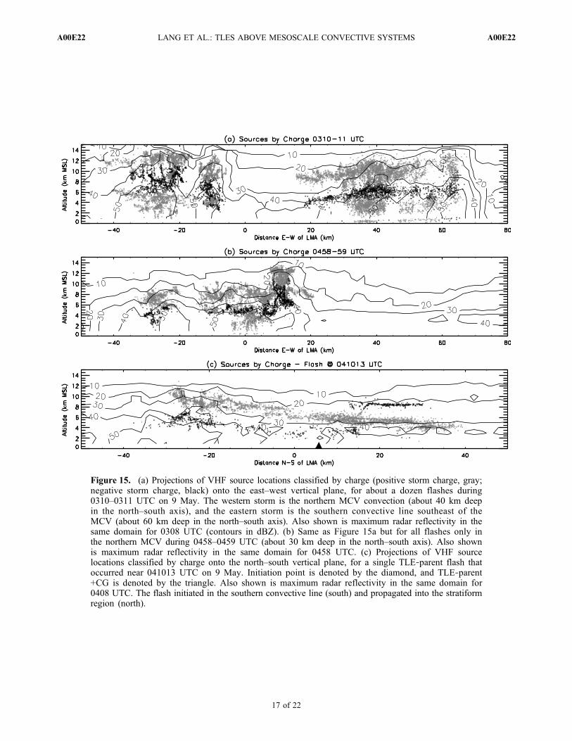
Figure 15. (a) Projections of VHF source locations classified by charge (positive storm charge, gray;negative storm charge, black) onto the east–west vertical plane, for about a dozen flashes during0310–0311 UTC on 9 May. The western storm is the northern MCV convection (about 40 km deepin the north–south axis), and the eastern storm is the southern convective line southeast of theMCV (about 60 km deep in the north–south axis). Also shown is maximum radar reflectivity in thesame domain for 0308 UTC (contours in dBZ). (b) Same as Figure 15a but for all flashes only inthe northern MCV during 0458–0459 UTC (about 30 km deep in the north–south axis). Also shownis maximum radar reflectivity in the same domain for 0458 UTC. (c) Projections of VHF sourcelocations classified by charge onto the north–south vertical plane, for a single TLE‐parent flash thatoccurred near 041013 UTC on 9 May. Initiation point is denoted by the diamond, and TLE‐parent+CG is denoted by the triangle. Also shown is maximum radar reflectivity in the same domain for0408 UTC. The flash initiated in the southern convective line (south) and propagated into the stratiformregion (north).

LANG ET AL.: TLES ABOVE MESOSCALE CONVECTIVE SYSTEMS A00E22A00E22

17 of 22

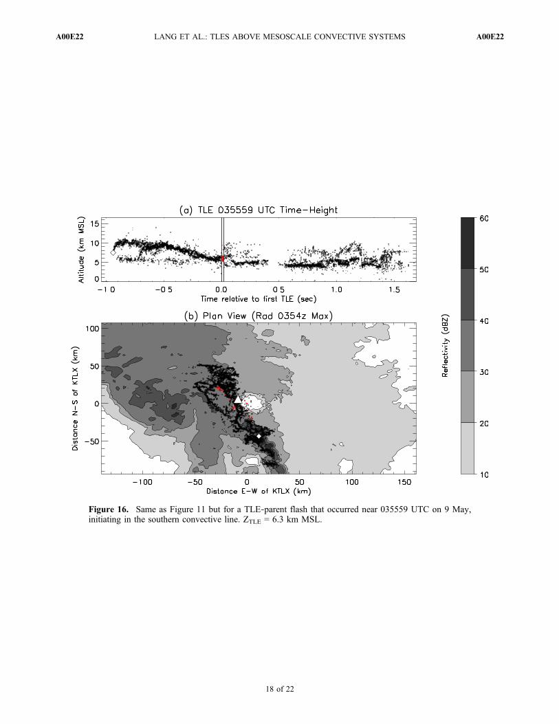
Figure 16. Same as Figure 11 but for a TLE‐parent flash that occurred near 035559 UTC on 9 May,initiating in the southern convective line. ZTLE = 6.3 km MSL.

LANG ET AL.: TLES ABOVE MESOSCALE CONVECTIVE SYSTEMS A00E22A00E22

18 of 22

[Parker and Johnson, 2000], need to be examined to clarifyhow sprite production, including the charge layer tapped bysprite parents, depends on MCS morphology.

Appendix A

[59] Given the lack of specificity in the MacGorman etal. [2008] mapping guidelines (3‐D “mapped well” within

100 km; 2‐D “mapped well” within 200 km), actual spatialerrors as a function of range from network center wereestimated using NMIMT‐developed software that integratedwith their XLMA software package (Figure A1). The timeperiod 0500–0510 UTC on 20 June was examined, as at thistime the convective line of the MCS was located over thecenter of the OK‐LMA network, providing 2,038,335 sour-ces over the widest possible set of ranges to examine. At100 km range, modeled vertical location error was 0.89 km,

Table 2. Mean Values for Various Parameters Associated withTLE‐Parent Flashes for 9 May, Broken Down by Flashes Initiatingin the Northern MCV and Southern Convective Linea

MCV‐Initiated Southern‐Initiated

SignificantlyDifferentat 90%+

Confidence?

Flashes 18 5 N/AZINIT (km MSL) 5.5 7.5 YesInitiation reflectivity

(dBZ)39.6 38.7 No

Peak current (kA) 57 68 NoCG reflectivity

(dBZ)44.8 49.9 Yes

Time to CG (s) 0.503 0.900 YesZTLE (km MSL) 6.2 5.9 NoFlash area (km2) 8185 9438 No

aSignificance testing was done using the nonparametric rank sum test[Walpole et al., 2002]. Subtract 0.4 km to convert ZTLE to Zq.

Table 3. Mean Values for Various Parameters Associated WithTLE‐Parent Flashes for 20 June 2007, 9 May 2007, and 19 July2000a

20 June 2007 9 May 2007 19 July 2000

Flashes 49 23 17ZINIT (km MSL) 7.7 5.9 N/AInitiation Reflectivity (dBZ) 35.7 39.5 N/APeak Current (kA) 76 59 68CG Reflectivity (dBZ) 41.7 46.5 N/ATime to CG (s) 1.201 0.589 N/AZTLE (km MSL) 8.2 6.1 5.2Flash Area (km2) 22,644 8458 4494

aLyons et al. [2003]. Lyons et al. [2003] values were updated to matchthe methodology used in the present study (ground level was 1.1 km MSLfor Lyons). All 9 May and 20 June parameters were significantly differentat 95%+ confidence using the nonparametric rank sum test [Walpole et al.,2002].

Figure 17. Same as Figure 11 but for a TLE‐parent flash that occurred near 031207 UTC on 9 May,initiating in the northern MCV convection. ZTLE = 5.5 km MSL.

LANG ET AL.: TLES ABOVE MESOSCALE CONVECTIVE SYSTEMS A00E22A00E22

19 of 22

while at 200 km range, the error was 2.13 km. Horizontallocation errors were less.[60] At 175 km range, vertical location error was 1.82 km,

which was not ideal for 3‐D flash analysis. However,these errors were nearly normally distributed [Thomas etal., 2004], and not all sources associated with the par-ent lightning were at this long range (though some werefurther depending on flash structure). Therefore, givenenough sources, there would be reduced uncertainty in anyderived mean locations. For example, the average 95%confidence interval for ZTLE values computed on 20 Junewas +/−0.3 km, and the absolute worst confidence intervalfor a 20 June ZTLE was +/−0.6 km. These values were muchbetter than the vertical location errors for individual sources.[61] There is the potential for overestimation of vertical

locations in long‐range LMA data, which can create anupward bias in any derived altitude parameter [Thomas etal., 2004]. To examine this possibility, ZTLE analyseswere recomputed for 20 June using a few different inde-pendent methodologies (Table A1). Examining only flasheswith the TLE‐parent +CG within 130 km of the OK‐LMA(which was within 1.25 km vertical error; Figure A1),average ZTLE was 8.2 km MSL, the same as flashes beyond130 km.[62] Another method was to consolidate all sources con-

tributing to ZTLE estimates among all flashes, instead oftreating TLE parents individually. This allowed thebreakdown of all sources within 100 km of the OK‐LMA,and all sources beyond that range. Once again, long‐rangeresults were only slightly higher in altitude (with onlyslightly worse standard deviations) than short‐range results(Table A1). Other alternative methodologies for calculatingZTLE, such as not utilizing the 30‐source rule (section 2.6.2),

or specifying a fixed time period after the TLE‐parent +CG(such as 100 ms), also did not change the results.[63] Additional special care was taken to ensure that

altitude estimates were correct for 20 June. In particular,objectively analyzed heights were compared with handanalysis of the same flashes. For example, the ZTLE para-meter’s value was visually compared to the vertical loca-tions of sources outside the defined time period (i.e., beforeand after the CG/TLE) to ensure that the estimate wasaccurate.[64] Based on this work, no serious problems were

found with the objective analyses on 20 June, and altitudeparameters derived for each flash are considered the mostaccurate possible. More specifically, the observed ZTLE

values on 20 June clearly were the result of discharging ofthe upper positive charge layer in the MCS during TLEproduction, and not an artifact of long‐range OK‐LMAobservations or an incorrect methodology for calculatingZTLE.

[65] Acknowledgments. The authors gratefully acknowledge ThomasNelson for serving as facilities manager for YRFS and for maintainingthe TLE monitoring equipment and database during Sprites 2007. RonThomas of NMIMT provided substantial assistance with assessing locationerrors by the OK‐LMA. Thomas Marshall of the University of Mississippiprovided helpful comments on this paper. Jingbo Li of Duke Universityprovided substantial assistance with the CMC data. WSR‐88D data wereobtained from the National Oceanic and Atmospheric Administration’sNational Climate Data Center. NLDN data were obtained from Vaisala,Inc. Sounding data were obtained from the University of Wyoming(http://weather.uwyo.edu/upperair/sounding.html). This research wasfunded by the National Science Foundation’s Physical Meteorology pro-gram via grant ATM‐0649034.[66] Amitava Bhattacharjee thanks Thomas Marshall and another

reviewer for their assistance in evaluating this paper.

ReferencesBell, T. F., V. P. Pasko, and U. S. Inan (1995), Runaway electrons as asource of red sprites in the mesosphere, Geophys. Res. Lett., 22(16),2127–2130, doi:10.1029/95GL02239.

Benjamin, S. G., et al. (2004a), An hourly assimilation–forecast cycle: TheRUC, Mon. Weather Rev., 132, 495–518, doi:10.1175/1520-0493(2004)132<0495:AHACTR>2.0.CO;2.

Benjamin, S. G., G. A. Grell, J. M. Brown, T. G. Smirnova, and R. Bleck(2004b), Mesoscale weather prediction with the RUC hybrid isentropic–terrain‐following coordinate model, Mon. Weather Rev., 132, 473–494,doi:10.1175/1520-0493(2004)132<0473:MWPWTR>2.0.CO;2.

Boccippio, D. J., E. R. Williams, W. A. Lyons, I. Baker, and R. Boldi(1995), Sprites, ELF transients and positive ground strokes, Science,269, 1088–1091, doi:10.1126/science.269.5227.1088.

Carey, L. D., M. J. Murphy, T. L. McCormick, and N. W. S. Demetriades(2005), Lightning location relative to storm structure in a leading‐line,

Table A1. Statistics for 20 June ZTLE Estimates Derived FromDifferent Techniquesa

MethodRange

CriterionNumber of

MeasurementsZTLE

(km MSL)

StandardDeviation(km)

Flashes treatedseparately

<130 km 13 flashes 8.2 0.8

>130 km 36 flashes 8.2 1.1ZTLE sources for all

flashes combinedtogether

<100 km 4262 sources 8.2 1.9

>100 km 7984 sources 8.3 2.0

aSubtract 0.4 km to convert ZTLE to Zq.

Figure A1. Linear fits via the least squares method toOK‐LMA VHF source location errors as functions of rangefor 2+ million sources observed during 0500–0510 UTC on20 June. Shown are errors for the vertical direction (Z; solidblack), east–west direction (X; dash black), and north–southdirection (Y; solid gray). Y errors were less than X becausethe storm was oriented approximately east–west, and azi-muthal errors are less than range errors with LMA systems[Thomas et al., 2004]. Correlation coefficients were 0.82 (X),0.70 (Y), and 0.63 (Z).

LANG ET AL.: TLES ABOVE MESOSCALE CONVECTIVE SYSTEMS A00E22A00E22

20 of 22

trailing‐stratiform mesoscale convective system, J. Geophys. Res., 110,D03105, doi:10.1029/2003JD004371.

Chauzy, S., M. Chong, A. Delannoy, and S. Despiau (1985), The June 22tropical squall line observed during COPT 81 experiment: Electrical sig-nature associated with dynamical structure and precipitation, J. Geophys.Res., 90(D4), 6091–6098, doi:10.1029/JD090iD04p06091.

Chen, A. B., et al. (2008), Global distributions and occurrence rates of tran-sient luminous events, J. Geophys. Res., 113, A08306, doi:10.1029/2008JA013101.

Coleman, L. M., T. C. Marshall, M. Stolzenburg, T. Hamlin, P. R. Krehbiel,W. Rison, and R. J. Thomas (2003), Effects of charge and electrostaticpotential on lightning propagation, J. Geophys. Res., 108(D9), 4298,doi:10.1029/2002JD002718.

Cressman, G. P. (1959), An operational objective analysis system, Mon.Weather Rev., 87, 367–374, doi:10.1175/1520-0493(1959)087<0367:AOOAS>2.0.CO;2.

Cummer, S. A., and U. S. Inan (1997), Measurement of charge transfer insprite‐producing lightning using ELF radio atmospherics, Geophys. Res.Lett., 24(14), 1731–1734, doi:10.1029/97GL51791.

Cummer, S. A., and W. A. Lyons (2004), Lightning charge momentchanges in U.S. High Plains thunderstorms, Geophys. Res. Lett., 31,L05114, doi:10.1029/2003GL019043.

Cummer, S. A., and W. A. Lyons (2005), Implications of lightning chargemoment changes for sprite initiation, J. Geophys. Res., 110, A04304,doi:10.1029/2004JA010812.

Cummins, K. L., M. J. Murphy, E. A. Bardo, W. L. Hiscox, R. B. Pyle, andA. E. Pifer (1998), A combined TOA/MDF technology upgrade of theU. S. National Lightning Detection Network, J. Geophys. Res., 103,9035–9044, doi:10.1029/98JD00153.

Davis, C., et al. (2004), The Bow Echo and MCV Experiment: Observa-tions and opportunities, Bull. Am. Meteorol. Soc., 85, 1075–1093,doi:10.1175/BAMS-85-8-1075.

Dotzek, N., R. M. Rabin, L. D. Carey, D. R. MacGorman, T. L. McCormick,N. W. Demetriades, M. J. Murphy, and R. L. Holle (2005), Lightningactivity related to satellite and radar observations of a mesoscale convec-tive system over Texas on 7–8 April 2002, Atmos. Res., 76, 127–166,doi:10.1016/j.atmosres.2004.11.020.

Ely, B. L., R. E. Orville, L. D. Carey, and C. L. Hodapp (2008), Evolutionof the total lightning structure in a leading‐line, trailing‐stratiform meso-scale convective system over Houston, Texas, J. Geophys. Res., 113,D08114, doi:10.1029/2007JD008445.

Houze, R. A., Jr., B. F. Smull, and P. Dodge (1990), Mesoscale organiza-tion of springtime rainstorms in Oklahoma, Mon. Weather Rev., 118,613–654, doi:10.1175/1520-0493(1990)118<0613:MOOSRI>2.0.CO;2.

Huang, E., E. Williams, R. Boldi, S. Heckman, W. Lyons, M. Taylor,T. Nelson, and C. Wong (1999), Criteria for sprites and elves based onSchumann resonance observations, J. Geophys. Res., 104, 16,943–16,964, doi:10.1029/1999JD900139.

Kasemir, H. W. (1960), A contribution to the electrostatic theory of a light-ning discharge, J. Geophys. Res., 65(7), 1873–1878, doi:10.1029/JZ065i007p01873.

Krehbiel, P. R., R. J. Thomas, W. Rison, T. Hamlin, J. Harlin, and M. Davis(2000), GPS‐based mapping system reveals lightning inside storms, EosTrans. AGU, 81, 21–25, doi:10.1029/00EO00014.

Lang, T. J., and S. A. Rutledge (2008), Kinematic, microphysical, andelectrical aspects of an asymmetric bow‐echo mesoscale convectivesystem observed during STEPS 2000, J. Geophys. Res., 113, D08213,doi:10.1029/2006JD007709.

Lang, T. J., S. A. Rutledge, and K. C. Wiens (2004), Origins of positivecloud‐to‐ground lightning flashes in the stratiform region of a mesoscaleconvective system, Geophys. Res. Lett., 31, L10105, doi:10.1029/2004GL019823.

Lu, G., S. A. Cummer, J. Li, F. Han, R. J. Blakeslee, and H. J. Christian(2009), Charge transfer and in‐cloud structure of large‐charge‐momentpositive lightning strokes in a mesoscale convective system, Geophys.Res. Lett., 36, L15805, doi:10.1029/2009GL038880.

Lyons, W. A. (1996), Sprite observations above the U.S. High Plains inrelation to their parent thunderstorm systems, J. Geophys. Res., 101,29,641–29,652, doi:10.1029/96JD01866.

Lyons, W. A. (2006), The meteorology of transient luminous events—Anintroduction and overview, in NATO Advanced Study Institute on Sprites,Elves and Intense Lightning Discharges, edited by M. Fullekrug et al.,pp. 19–56, Springer, New York.

Lyons, W. A., T. E. Nelson, E. R. Williams, S. A. Cummer, and M. A.Stanley (2003), Characteristics of sprite‐producing positive cloud‐to‐ground lightning during the 19 July 2000 STEPS mesoscale convectivesystems, Mon. Weather Rev., 131, 2417–2427, doi:10.1175/1520-0493(2003)131<2417:COSPCL>2.0.CO;2.

Lyons, W. A., L. M. Andersen, T. E. Nelson, and G. R. Huffines (2006),Characteristics of sprite‐producing electrical storms in the STEPS 2000domain, paper presented at Second Conference on Meteorological Appli-cations of Lightning Data, Am. Meteorol. Soc., Atlanta, Ga.

Lyons, W. A., S. A. Cummer, M. A. Stanley, G. R. Huffines, K. C. Wiens,and T. E. Nelson (2008), Supercells and sprites, Bull. Am. Meteorol. Soc.,89, 1165–1174, doi:10.1175/2008BAMS2439.1.

Lyons, W. A., M. Stanley, J. D. Meyer, T. E. Nelson, S. A. Rutledge, T. J.Lang, and S. A. Cummer (2009), The meteorological and electrical struc-ture of TLE‐producing convective storms, in Lightning: Principles,Instruments and Applications, edited by H. D. Betz et al., pp. 389–417, doi:10.1007/978-1-4020-9079-0_17, Springer, New York.

MacGorman, D. R., W. D. Rust, P. Krehbiel, W. Rison, E. Bruning, andK. Wiens (2005), The electrical structure of two supercell storms duringSTEPS, Mon. Weather Rev., 133, 2583–2607, doi:10.1175/MWR2994.1.

MacGorman, D. R., et al. (2008), TELEX The Thunderstorm Electrificationand Lightning Experiment, Bull. Am. Meteorol. Soc., 89, 997–1013,doi:10.1175/2007BAMS2352.1.

Maddox, R. A. (1980), Mesoscale convective complexes, Bull. Am. Meteorol.Soc., 61, 1374–1387, doi:10.1175/1520-0477(1980)061<1374:MCC>2.0.CO;2.

Marshall, T. C., and W. D. Rust (1993), Two types of vertical electricalstructures in stratiform precipitation regions of mesoscale convective sys-tems, Bull. Am. Meteorol. Soc., 74, 2159–2170, doi:10.1175/1520-0477(1993)074<2159:TTOVES>2.0.CO;2.

Marshall, T. C., W. D. Rust, W. P. Winn, and K. E. Gilbert (1989), Elec-trical structure in two thunderstorm anvil clouds, J. Geophys. Res., 94,2171–2181, doi:10.1029/JD094iD02p02171.

Marshall, T. C., M. Stolzenburg, and W. D. Rust (1996), Electric fieldmeasurements above mesoscale convective systems, J. Geophys. Res.,101(D3), 6979–6996, doi:10.1029/95JD03764.

Marshall, T. C., M. Stolzenburg, W. D. Rust, E. R. Williams, and R. Boldi(2001), Positive charge in the stratiform cloud of a mesoscale con-vective system, J. Geophys. Res., 106(D1), 1157–1163, doi:10.1029/2000JD900625.

Mazur, V., and L. H. Ruhnke (1993), Common physical processes innatural and artificially triggered lightning, J. Geophys. Res., 98,12,913–12,930, doi:10.1029/93JD00626.

Mazur, V., P. R. Krehbiel, and X.‐M. Shao (1995), Correlated high‐speedvideo and interferometric observations of a cloud‐to‐ground lightningflash, J. Geophys. Res., 100, 25,731–25,753, doi:10.1029/95JD02364.

Mazur, V., X.‐M. Shao, and P. R. Krehbiel (1998), “Spider” lightning inintracloud and positive cloud‐to‐ground flashes, J. Geophys. Res., 103,19,811–19,822, doi:10.1029/98JD02003.

Parker, M. D., and R. H. Johnson (2000), Organizational modes of midlat-itude mesoscale convective systems, Mon. Weather Rev., 128, 3413–3436, doi:10.1175/1520-0493(2001)129<3413:OMOMMC>2.0.CO;2.

Pasko, V. P., U. S. Inan, Y. N. Taranenko, and T. F. Bell (1995), Heating,ionization and upward discharges in the mesosphere, due to intensequasi‐electrostatic thundercloud fields, Geophys. Res. Lett., 22(4),365–368, doi:10.1029/95GL00008.

Pasko, V. P., U. S. Inan, and T. F. Bell (1996), Sprites as luminous col-umns of ionization produced by quasi‐electrostatic thundercloud fields,Geophys. Res. Lett., 23, 649–652, doi:10.1029/96GL00473.

Pasko, V. A., U. S. Inan, T. F. Bell, and Y. N. Taranenko (1997), Spritesproduced by quasi‐electrostatic heating and ionization in the lower iono-sphere, J. Geophys. Res., 102(A3), 4529–4561, doi:10.1029/96JA03528.

Rison, W., R. J. Thomas, P. R. Krehbiel, T. Hamlin, and J. Harlin (1999),A GPS‐based three‐dimensional lightning mapping system: Initial obser-vations in central New Mexico, Geophys. Res. Lett., 26, 3573–3576,doi:10.1029/1999GL010856.

Roussel‐Dupré, R., and A. V. Gurevich (1996), On runaway breakdownand upward propagating discharges, J. Geophys. Res., 101(A2), 2297–2311, doi:10.1029/95JA03278.

Rust, W. D., D. R. MacGorman, E. C. Buning, S. A. Weiss, P. R. Krehbiel,R. J. Thomas, W. Rison, and J. Harlin (2005), Inverted‐polarity electricalstructures in thunderstorms in the Severe Thunderstorm ElectrificationStudy (STEPS), Atmos. Res., 76, 247–271, doi:10.1016/j.atmosres.2004.11.029.

Rutledge, S. A., and D. R. MacGorman (1988), Cloud‐to‐ground lightningactivity in the 10–11 June 1985 mesoscale convective system observedduring the Oklahoma‐Kansas PRE‐STORM project, Mon. WeatherRev., 116, 1393–1408, doi:10.1175/1520-0493(1988)116<1393:CTGLAI>2.0.CO;2.

Rutledge, S. A., and W. A. Petersen (1994), Vertical radar reflectivity struc-ture and cloud‐to‐ground lightning in the stratiform region of MCSs:Further evidence for in situ charging in the stratiform region, Mon.Weather Rev., 122, 1760–1776, doi:10.1175/1520-0493(1994)122<1760:VRRSAC>2.0.CO;2.

LANG ET AL.: TLES ABOVE MESOSCALE CONVECTIVE SYSTEMS A00E22A00E22

21 of 22

Rutledge, S. A., C. Lu, and D. R. MacGorman (1990), Positive cloud‐to‐ground lightning in mesoscale convective systems, J. Atmos. Sci., 47,2085–2100, doi:10.1175/1520-0469(1990)047<2085:PCTGLI>2.0.CO;2.

Schuur, T. J., and S. A. Rutledge (2000a), Electrification of stratiformregions in mesoscale convective systems. Part I: An observational com-parison of symmetric and asymmetric MCSs, J. Atmos. Sci., 57, 1961–1982, doi:10.1175/1520-0469(2000)057<1961:EOSRIM>2.0.CO;2.

Schuur, T. J., and S. A. Rutledge (2000b), Electrification of stratiformregions in mesoscale convective systems. Part II: Two‐dimensionalnumerical model simulations of a symmetric MCS, J. Atmos. Sci., 57,1983–2006, doi:10.1175/1520-0469(2000)057<1983:EOSRIM>2.0.CO;2.

Schuur, T. J., W. D. Rust, B. F. Smull, and T. C. Marshall (1991), Electri-cal and kinematic structure of the stratiform precipitation region trailingan Oklahoma squall line, J. Atmos. Sci., 48, 825–842, doi:10.1175/1520-0469(1991)048<0825:EAKSOT>2.0.CO;2.

Scott, J. D., and S. A. Rutledge (1995), Doppler radar observations of anasymmetric mesoscale convective system and associated vortex couplet,Mon. Weather Rev., 123, 3437–3457, doi:10.1175/1520-0493(1995)123<3437:DROOAA>2.0.CO;2.

Shepherd, T. R., W. D. Rust, and T. C. Marshall (1996), Electric fields andcharges near 0°C in stratiform clouds,Mon. Weather Rev., 124, 919–938,doi:10.1175/1520-0493(1996)124<0919:EFACNI>2.0.CO;2.

Smull, B. F., and R. A. Houze (1985), A midlatitude squall line with a trail-ing region of stratiform rain: Radar and satellite observations, Mon.Weather Rev., 113, 117–133, doi:10.1175/1520-0493(1985)113<0117:AMSLWA>2.0.CO;2.

Stanley, M., P. Krehbiel, M. Brook, C. Moore, and W. Rison (1999), Highspeed video of initial sprite development, Geophys. Res. Lett., 26, 3201–3204, doi:10.1029/1999GL010673.

Steiger, S. M., R. E. Orville, and L. D. Carey (2007), Total lightning sig-natures of thunderstorm intensity over north Texas. Part II: Mesoscaleconvective systems, Mon. Weather Rev., 135, 3303–3324, doi:10.1175/MWR3483.1.

Stolzenburg, M., T. C. Marshall, W. D. Rust, and B. F. Smull (1994),Horizontal distribution of electrical and meteorological conditionsacross the stratiform region of a mesoscale convective system, Mon.Weather Rev., 122, 1777–1797, doi:10.1175/1520-0493(1994)122<1777:HDOEAM>2.0.CO;2.

Stolzenburg, M., W. D. Rust, B. F. Smull, and T. C. Marshall (1998), Elec-trical structure in thunderstorm convective regions: 1. Mesoscale convec-tive systems, J. Geophys. Res., 103, 14,059–14,078, doi:10.1029/97JD03546.

Stolzenburg, M., T. C. Marshall, and W. D. Rust (2001), Serial soundingsof electric field through the mesoscale convective system, J. Geophys.Res., 106, 12,371–12,380, doi:10.1029/2001JD900074.

Thomas, R., P. Krehbiel, W. Rison, J. Harlin, T. Hamlin, and N. Campbell(2003), The LMA flash algorithm, paper presented at 11th International

Conference on Atmospheric Electricity, pp. 655–656, Int. Comm. onAtmos. Electr., Versailles, France.

Thomas, R. J., P. R. Krehbiel, W. Rison, S. J. Hunyady, W. P. Winn,T. Hamlin, and J. Harlin (2004), Accuracy of the Lightning MappingArray, J. Geophys. Res., 109, D14207, doi:10.1029/2004JD004549.

Walpole, R. E., R. H. Meyers, S. L. Myers, and K. Ye (2002), Probabilityand Statistics for Scientists and Engineers, 7th ed., 730 pp., PrenticeHall, Upper Saddle River, N. J.

Wiens, K. C., S. A. Rutledge, and S. A. Tessendorf (2005), The 29 June2000 supercell observed during STEPS. Part II: Lightning and chargestructure, J. Atmos. Sci., 62, 4151–4177, doi:10.1175/JAS3615.1.

Williams, E. R. (1998), The positive charge reservoir for sprite‐producinglightning, J. Atmos. Sol. Terr. Phys., 60, 689–692, doi:10.1016/S1364-6826(98)00030-3.

Williams, E. R. (2001), Sprites, elves and glow discharge tubes, Phys.Today, 54, 41–47, doi:10.1063/1.1428435.

Williams, E. R., and Y. Yair (2006), The microphysical and electricalproperties of sprite‐producing thunderstorms, in NATO Advanced StudyInstitute on Sprites, Elves and Intense Lightning Discharges, edited byM. Fullekrug et al., pp. 57–83, Springer, New York.

Williams, E., B. Boldi, A. Matlin, M. Weber, S. Hodanish, D. Sharp,S. Goodman, R. Raghavan, and D. Buechler (1999), The behavior oftotal lightning activity in severe Florida thunderstorms, Atmos. Res.,51, 245–265, doi:10.1016/S0169-8095(99)00011-3.

Wilson, C. T. R. (1924), The electric field of a thunderstorm and some ofits effects, Proc. Phys. Soc. London, 37, 32D–37D, doi:10.1088/1478-7814/37/1/314.

Yuter, S. E., and R. A. Houze Jr. (1998), The natural variability of precip-itating clouds over the western Pacific warm pool, Q. J. R. Meteorol.Soc., 124, 53–99, doi:10.1002/qj.49712454504.

Zhang, J., K. Howard, and J. J. Gourley (2005), Constructing three‐dimensional multiple‐radar reflectivity mosaics: Examples of convectivestorms and stratiform rain echoes, J. Atmos. Oceanic Technol., 22, 30–42, doi:10.1175/JTECH-1689.1.

S. A. Cummer, Department of Electrical Engineering, Duke University,PO Box 90291, Durham, NC 27708, USA.T. J. Lang and S. A. Rutledge, Department of Atmospheric Science,

Colorado State University, 200 W. Lake St. Fort Collins, CO 80523,USA. (tlang@atmos.colostate.edu)W. A. Lyons, FMA Research, Inc., 46050 Weld County Rd. 13, Fort

Collins, CO 80524, USA.D. R. MacGorman, National Severe Storms Laboratory, CIMMS/Room

1110, 100 E. Boyd, Norman, OK 73069, USA.J. D. Meyer, Department of Atmospheric Sciences, South Dakota School

of Mines and Technology, 501 East Saint Joseph St., Rapid City, SD 57701,USA.

LANG ET AL.: TLES ABOVE MESOSCALE CONVECTIVE SYSTEMS A00E22A00E22

22 of 22