TRANSFORMATION OF RENDERING ALGORITHMS FOR …sirkan.iit.bme.hu/~szirmay/abbas.pdfTRANSFORMATION OF...

TRANSFORMATIONOF RENDERING ALGORITHMS

FOR HARDWARE IMPLEMENTATION

Ph.D. Thesis byAli Mohamed Ali Abbas

scientific supervisorProfessor Dr. Szirmay-Kalos Laszlo

Faculty of Electrical Engineering and InformaticsBudapest University of Technology and Economics

Budapest, ��

Contents

1 Introduction 11.1 Tasks of image synthesis . . . . . . . . . . . . . . . . . . . . . . . . . . . . . . . . . . 41.2 Incremental shading techniques . . . . . . . . . . . . . . . . . . . . . . . . . . . . . . . 7

1.2.1 Rasterization . . . . . . . . . . . . . . . . . . . . . . . . . . . . . . . . . . . . 81.3 The objectives of this thesis . . . . . . . . . . . . . . . . . . . . . . . . . . . . . . . . . 10

2 Hardware implementation of rendering functions 112.1 Functions on scan-lines . . . . . . . . . . . . . . . . . . . . . . . . . . . . . . . . . . . 11

2.1.1 One-variate constant functions . . . . . . . . . . . . . . . . . . . . . . . . . . . 112.1.2 One-variate linear functions . . . . . . . . . . . . . . . . . . . . . . . . . . . . 122.1.3 One-variate quadratic functions . . . . . . . . . . . . . . . . . . . . . . . . . . 13

2.2 Functions on triangles . . . . . . . . . . . . . . . . . . . . . . . . . . . . . . . . . . . . 142.2.1 Two-variate constant functions . . . . . . . . . . . . . . . . . . . . . . . . . . . 152.2.2 Two-variate linear functions . . . . . . . . . . . . . . . . . . . . . . . . . . . . 162.2.3 Two-variate quadratic functions . . . . . . . . . . . . . . . . . . . . . . . . . . 18

3 Drawing lines 213.1 Bresenham algorithm . . . . . . . . . . . . . . . . . . . . . . . . . . . . . . . . . . . . 21

3.1.1 Hardware implementation of Bresenham’s line-drawing algorithm . . . . . . . . 243.2 Anti-aliasing lines . . . . . . . . . . . . . . . . . . . . . . . . . . . . . . . . . . . . . . 26

3.2.1 Box-filtering lines . . . . . . . . . . . . . . . . . . . . . . . . . . . . . . . . . 263.2.2 Incremental cone-filtering lines . . . . . . . . . . . . . . . . . . . . . . . . . . 283.2.3 Hardware implementation of incremental cone-filtering lines . . . . . . . . . . . 31

3.3 Depth cueing . . . . . . . . . . . . . . . . . . . . . . . . . . . . . . . . . . . . . . . . 35

4 Shaded surface rendering with linear interpolation 364.1 Rasterizing an image space triangle . . . . . . . . . . . . . . . . . . . . . . . . . . . . 364.2 Linear interpolation on a triangle . . . . . . . . . . . . . . . . . . . . . . . . . . . . . . 37

4.2.1 2D linear interpolation . . . . . . . . . . . . . . . . . . . . . . . . . . . . . . . 384.2.2 Using a sequence of 1D linear interpolations . . . . . . . . . . . . . . . . . . . 384.2.3 Interpolation with blending functions . . . . . . . . . . . . . . . . . . . . . . . 39

4.3 An image space hidden surface elimination algorithm: the z-buffer algorithm . . . . . . 394.3.1 Hardware implementation of z-buffer algorithm . . . . . . . . . . . . . . . . . . 40

4.4 Incremental shading algorithms . . . . . . . . . . . . . . . . . . . . . . . . . . . . . . . 424.4.1 Constant shading . . . . . . . . . . . . . . . . . . . . . . . . . . . . . . . . . . 434.4.2 Gouraud shading . . . . . . . . . . . . . . . . . . . . . . . . . . . . . . . . . . 43

i

CONTENTS ii

4.5 Hardware implementation of Gouraud shading and z-buffer algorithms . . . . . . . . . . 44

5 Drawing triangles with Phong shading 475.1 Normals shading . . . . . . . . . . . . . . . . . . . . . . . . . . . . . . . . . . . . . . 485.2 Dot product interpolation . . . . . . . . . . . . . . . . . . . . . . . . . . . . . . . . . . 495.3 Polar angles interpolation . . . . . . . . . . . . . . . . . . . . . . . . . . . . . . . . . . 495.4 Angular interpolation . . . . . . . . . . . . . . . . . . . . . . . . . . . . . . . . . . . . 495.5 Phong shading and Taylor’s series approximation . . . . . . . . . . . . . . . . . . . . . 51

5.5.1 Diffuse part for directional light sources . . . . . . . . . . . . . . . . . . . . . . 525.5.2 Specular part for directional light sources . . . . . . . . . . . . . . . . . . . . . 53

6 Spherical interpolation 546.1 Independent spherical interpolation of a pair of vectors . . . . . . . . . . . . . . . . . . 556.2 Simultaneous spherical interpolation of a pair of vectors . . . . . . . . . . . . . . . . . 566.3 Interpolation and Blinn BRDF calculation by hardware . . . . . . . . . . . . . . . . . . 576.4 Simulation results . . . . . . . . . . . . . . . . . . . . . . . . . . . . . . . . . . . . . . 63

7 Quadratic interpolation 657.1 Error control . . . . . . . . . . . . . . . . . . . . . . . . . . . . . . . . . . . . . . . . . 677.2 Hardware implementation of quadratic interpolation . . . . . . . . . . . . . . . . . . . . 687.3 Simulation results . . . . . . . . . . . . . . . . . . . . . . . . . . . . . . . . . . . . . . 69

8 Texture mapping 728.1 Quadratic texturing . . . . . . . . . . . . . . . . . . . . . . . . . . . . . . . . . . . . . 738.2 Simulation results . . . . . . . . . . . . . . . . . . . . . . . . . . . . . . . . . . . . . . 74

9 Shaded surface rendering using global illumination 759.1 The global illumination problem . . . . . . . . . . . . . . . . . . . . . . . . . . . . . . 759.2 Ray-bundle based transfer . . . . . . . . . . . . . . . . . . . . . . . . . . . . . . . . . 769.3 Calculation of the radiance transport in a single direction . . . . . . . . . . . . . . . . . 789.4 Hardware implementation of the proposed radiance transfer algorithm . . . . . . . . . . 79

10 Conclusions and summary of new results 8210.1 General framework to compute simple functions on 2D triangles . . . . . . . . . . . . . 8210.2 Hardware implementation of incremental cone-filtering lines . . . . . . . . . . . . . . . 8310.3 Hardware implementation of Phong shading using spherical interpolation . . . . . . . . 8310.4 Quadratic interpolation in rendering . . . . . . . . . . . . . . . . . . . . . . . . . . . . 83

10.4.1 Adaptive error control in quadratic interpolation . . . . . . . . . . . . . . . . . 8410.4.2 Application of quadratic rendering for Phong shading and texture mapping . . . 84

10.5 Hardware implementation of global illumination . . . . . . . . . . . . . . . . . . . . . . 8710.6 Suggestions of future research . . . . . . . . . . . . . . . . . . . . . . . . . . . . . . . 87

BIBLIOGRAPHY 88

List of Figures

1.1 Tasks of rendering . . . . . . . . . . . . . . . . . . . . . . . . . . . . . . . . . 11.2 Geometry of the rendering equation . . . . . . . . . . . . . . . . . . . . . . . 21.3 Diffuse reflection . . . . . . . . . . . . . . . . . . . . . . . . . . . . . . . . . 31.4 Specular reflection . . . . . . . . . . . . . . . . . . . . . . . . . . . . . . . . 31.5 The evolution of the image . . . . . . . . . . . . . . . . . . . . . . . . . . . . 61.6 Dataflow of image synthesis . . . . . . . . . . . . . . . . . . . . . . . . . . . 71.7 Radiance calculation in local illumination methods . . . . . . . . . . . . . . . 71.8 Ambient, diffuse, and specular reflections . . . . . . . . . . . . . . . . . . . . 91.9 Comparison of linear interpolation i.e. Gouraud shading (left) and non-linear

interpolation by Phong shading (right) . . . . . . . . . . . . . . . . . . . . . . 10

2.1 Hardware implementation of one-variate constant functions . . . . . . . . . . . 122.2 Hardware implementation of one-variate linear functions . . . . . . . . . . . . 132.3 Hardware implementation of one-variate quadratic functions . . . . . . . . . . 142.4 Image space triangle and horizontal sided triangle . . . . . . . . . . . . . . . . 152.5 Hardware implementation of two-variate constant functions (left) and a raster

grid (right) . . . . . . . . . . . . . . . . . . . . . . . . . . . . . . . . . . . . . 162.6 Hardware implementation of two-variate linear functions . . . . . . . . . . . . 172.7 Hardware implementation of two-variate quadratic functions . . . . . . . . . . 19

3.1 Pixel grid for Bresenham’s Midpoint based line generator . . . . . . . . . . . . 223.2 Hardware implementation of Bresenhame’s line-drawing algorithm . . . . . . . 253.3 Time sequence of the hardware implementation of Bresenhame’s line-drawing

algorithm . . . . . . . . . . . . . . . . . . . . . . . . . . . . . . . . . . . . . 253.4 Box filtering of a line segment . . . . . . . . . . . . . . . . . . . . . . . . . . 263.5 Cone-filtering of a line segment . . . . . . . . . . . . . . . . . . . . . . . . . 283.6 Precomputed � �� weight tables . . . . . . . . . . . . . . . . . . . . . . . . 293.7 Incremental calculation of distance � . . . . . . . . . . . . . . . . . . . . . . 293.8 Hardware implementation of incremental cone-filtering lines . . . . . . . . . . 323.9 The time sequences of incremental cone-filtering lines . . . . . . . . . . . . . 333.10 The overlapped operations in the hardware of incremental cone-filtering lines . 333.11 Comparison of lines drawn by Bresenham’s algorithm (bottom), box-filtering

(middle) and the incremental cone-filtering (top) . . . . . . . . . . . . . . . . . 34

iii

LIST OF FIGURES iv

3.12 Comparison of coarsely tessellated wire-frame spheres (�� triangles) drawn byBresenham’s algorithm (left), box-filtering (middle) and the incremental cone-filtering (right) . . . . . . . . . . . . . . . . . . . . . . . . . . . . . . . . . . 34

3.13 Comparison of coarsely tessellated wire-frame spheres (�� triangles) hiddensurface removed, without depth-cueing (left) and with depth-cueing (right) . . . 35

4.1 Transformation to the screen coordinate system . . . . . . . . . . . . . . . . . 374.2 Linear interpolation on a triangle . . . . . . . . . . . . . . . . . . . . . . . . . 374.3 Screen space triangle . . . . . . . . . . . . . . . . . . . . . . . . . . . . . . . 414.4 Incremental concept in z-buffer calculations . . . . . . . . . . . . . . . . . . . 414.5 Hardware implementation of Gouraud shading and z-buffer algorithms . . . . . 454.6 Timing diagram of the hardware implementation of Gouraud shading and z-

buffer algorithms . . . . . . . . . . . . . . . . . . . . . . . . . . . . . . . . . 454.7 An interpolation of color in a triangle, with constant and Gouraud shadings . . 46

5.1 Comparison of linear and spherical interpolation of direction vectors . . . . . . 505.2 Vectors and angles variations along the mapped scan-line on two circular paths 51

6.1 Interpolation of vectors on a unit sphere . . . . . . . . . . . . . . . . . . . . . 546.2 Interpolation of two vectors . . . . . . . . . . . . . . . . . . . . . . . . . . . . 566.3 The bell shapes of �� for � � � �� (left) and of �� for

� � �� (right) . . . . . . . . . . . . . . . . . . . . . . . . . . . . 586.4 Approximation of �� by �� . . . . . . . . . . . . . . . . . . . . . . . 606.5 Quantization errors of the �� function for � and � address/data bits verses

the origonal �� function . . . . . . . . . . . . . . . . . . . . . . . . . . . . 616.6 Hardware implementation of Phong shading using spherical interpolation . . . 626.7 Timing diagram of the hardware of Phong shading using spherical interpolation 626.8 Evaluation of the visual accuracy approximation of the functions �� (left)

� �� (right). The shine (�) parameters of the rendered spheres are , �and �� . . . . . . . . . . . . . . . . . . . . . . . . . . . . . . . . . . . . . . . 63

6.9 Rendering of coarsely tessellated spheres with the proposed spherical interpo-lation, � bit precision (left) and � bit precision (right) . . . . . . . . . . . . . . 64

6.10 The mesh of a chicken (left) and its image rendered by classical Phong shading(middle) and by the proposed spherical interpolation (right) . . . . . . . . . . . 64

7.1 Highlight test and adaptive subdivision . . . . . . . . . . . . . . . . . . . . . . 677.2 Timing diagram of the hardware implementation of quadratic shading . . . . . 707.3 Rendering of coarsely tessellated spheres (�� triangles) of specular exponents

� � (top), � � �� (middle) and � � � (bottom) with Gouraud shading (left),quadratic shading (middle) and Phong shading (right) . . . . . . . . . . . . . . 70

7.4 Rendering of normal tessellated spheres (� � triangles) of specular exponents� � (top), � � �� (middle) and � � � (bottom) with Gouraud shading (left),quadratic shading (middle) and Phong shading (right) . . . . . . . . . . . . . . 71

LIST OF FIGURES v

7.5 Rendering of highly tessellated spheres (�� triangles) of specular exponents� � (top), � � �� (middle) and � � � (bottom) with Gouraud shading (left),quadratic shading (middle) and Phong shading (right) . . . . . . . . . . . . . . 71

8.1 Survey of texture mapping . . . . . . . . . . . . . . . . . . . . . . . . . . . . 738.2 Texture mapping with linear (left), quadratic (right) texture transformation . . . 74

9.1 Interpretation of �� . . . . . . . . . . . . . . . . . . . . . . . . . . . . 779.2 Global visibility algorithms . . . . . . . . . . . . . . . . . . . . . . . . . . . . 789.3 Scene as seen from two subsequent patches . . . . . . . . . . . . . . . . . . . 789.4 Organization of the transillumination buffer . . . . . . . . . . . . . . . . . . . 799.5 Hardware implementation of radiance transfer algorithm . . . . . . . . . . . . 819.6 Stage one time sequence of the hardware implementation of radiance transfer

algorithm . . . . . . . . . . . . . . . . . . . . . . . . . . . . . . . . . . . . . 81

10.1 Conventional rendering with Phong shading and texture mapping without inter-polation . . . . . . . . . . . . . . . . . . . . . . . . . . . . . . . . . . . . . . 84

10.2 Linear interpolation, i.e. Gouraud shading and linear texture mapping . . . . . 8510.3 Quadratic rendering . . . . . . . . . . . . . . . . . . . . . . . . . . . . . . . . 8510.4 A shaded pawn with Gouraud (left), Phong (middle) and Quadratic (right) . . . 8610.5 A shaded and textured apple with Gouraud (left), Phong (middle) and Quadratic

(right) . . . . . . . . . . . . . . . . . . . . . . . . . . . . . . . . . . . . . . . 8610.6 Coarsely tessellated, shaded, textured and specular tiger with Gouraud (left)

Phong (middle) and quadratic (right) . . . . . . . . . . . . . . . . . . . . . . . 86

Common abbreviations and notations

BRDF (��) Bi-Directional Reflection and Refraction FunctionCAD Computer Aided DesignFPGA Field Programmable Gate ArrayVHDL Hardware Description Language�� Local or world coordinates of �� and � respectively�� Screen coordinates of �� and � respectively�� Tristimulus color values, stands for red, green and blue respectively� Lighting direction� Surface normal� Reflection direction of � onto �� Viewing direction� Halfway vector between � and �� Surface point�� Ambient intensity�� Surface self-emission�� Radiance function of point � into direction �� Incoming radiance generated by light source �� Outgoing radiance�� Visibility function� Light transport operator� Directional hemisphere�� Differential solid angle at �� The angle between � and �

Æ The angle between � and �

� The angle between � and �� Ambient reflection parameter�� Diffuse reflection parameter�� Specular reflection parameter� Running variable

vi

Preface

Computer graphics basically aims at rendering complex virtual world models and presentingimages on a computer screen. To obtain an image of a virtual world, surfaces visible in pixelsshould be determined, and the rendering equation is used to calculate the color values of thepixels. The rendering equation, even in its simplified form, contains a lot of complex opera-tions, including the computation of the vectors, their normalization and the evaluation of theoutput radiance, which makes the process rather resource demanding. A real-time animationsystem has to generate at least images per second to provide the illusion of continuous mo-tion. Suppose that the number of pixels on the screen is about �� (advanced systems usuallyhave �� resolution). Thus the maximum average time to manipulate a single pixel,which might include visibility and rendering calculations, cannot exceed the following limit: � � �� !"#. Since this value is comparable to a few commercial memory read orwrite cycles, processors which execute programs by reading the instructions and the data frommemories are far too slow for this task, thus special solutions are needed. One alternative is thehardware realization, i.e. the design of a special digital network.

Hardware realization requires the original algorithms to be transformed to use only simpleoperations that are supported by the hardware elements. The idea behind this is to carry outthe expensive computations just for a few points or pixels, and the rest can be approximatedfrom these representative points by much simpler expressions using incremental evaluation.One way of doing this is the tessellation of the original surfaces to polygon meshes and usingthe vertices of the polygons as representative points. These techniques are based on linear(or in the extreme case, constant) interpolation. These methods are particularly efficient if thegeometric properties can also be determined in a similar way, connecting incremental shadingto the incremental visibility calculations of polygon mesh models.

Of course, when speeding up the algorithms, we cannot allow significant decrease of therealism. For example, the jaggies, which are common in all raster graphics systems should bereduced, which is called the anti-aliasing. The surfaces usually do not have constant materialproperties, but patterns or textures may appear. Such phenomena should also be handled by thegraphics system, which is the area of texture mapping. Sometimes it is not enough to computeonly the direct reflection of the light, but multiple reflections should also be taken into account.The family of algorithms that are capable of doing this is called global illumination.

This thesis contributes to the state of the art of rendering by proposing new rendering al-gorithms that overcome the drawbacks of linear interpolations and are comparable in imagequality with the already known sophisticated techniques but allow for simple hardware imple-mentation. These algorithms include the filtered line drawing, Phong shading, texture mapping

vii

LIST OF FIGURES viii

and ray-bundle based global illumination.The thesis is organized as follows:

� Chapter 1 is an introductory part to image synthesis process.

� Chapter 2 is a survey of various functions on scan-lines and triangles.

� Chapter 3 focuses on some line drawing algorithms, application of some filtering tech-niques and introduces a new approach called “incremental cone-filtering lines”.

� Chapter 4 is a survey of linear interpolation on triangles, visibility calculations based onthe z-buffer algorithm and an overview of constant and Gouraud shading methods.

� Chapter 5 is an overview of Phong shading and its related methods, such as normalsshading, dot product, angular shading, etc.

� Chapter 6 introduces a new shading algorithm based on “spherical interpolation” as analternative to Phong shading.

� Chapter 7 introduces a new method called “quadratic shading”.

� Chapter 8 is an overview of texture mapping and includes the application of our newmethod “quadratic interpolation” for this task.

� Chapter 9 focuses on ray-bundle global illumination and its hardware implementation.

� Chapter 10 contains the conclusions and the summary of the new results.

Acknowledgments

In the name of God, I wish to express my sincere gratitude to all who contributed their time,talent, knowledge, support and encouragement, for the completion of this work, in particular to:

My advisor and scientific supervisor, Professor Dr. Szirmay-Kalos Laszlo, for his advice,support and encouragement.

Dr. Horvath Tamas and Mr. Foris Tibor, for providing the valuable knowledge on program-ming and simulation environments.

Professor Dr. Arato Peter (Head of the Department and Dean of the Faculty), for his en-couragement and offering the pleasant research atmosphere.

Academic, technical and administrative staff at the Department of Control Engineering andInformation Technology, for their assistance during my study period.

Members in charge at the Faculty: Professor Dr. Selenyi Endre (Vice-Dean of scientificaffairs), Dr. Harangozo, Jozsef (Ph.D. course director) and Dr. Zoltai Jozsef (Vice-Dean ofstudent affairs), for their excellent cooperation during my study period.

Members in charge at the International Education Center: Dr. Gyula Csopaki (Director),Dr. Logo Janos (Libyan students affairs coordinator) and Mrs. Nagy Margit (administrativecoordinator), for their excellent cooperation during my study period.

My parents, my wife and my five children, for their encouragement, support and patience.

Libyan society, for the financial support.

Budapest, ��. Ali Mohamed Ali Abbas

ix

Chapter 1

Introduction

The objective of image synthesisor rendering is to provide the user with the illusion of watch-ing real objects on the computer screen. The image is generated from an internal model that iscalled the virtual world . To provide the illusion of watching the real world, the color sensationof an observer looking at the artificial image generated by the graphics system must be similarto the color perception which would be obtained in the real world (Figure 1.1).

Tonemapping

R

G

B

RadiancePower

Radiance

Power

λλ

λ

λ

Power

λ

Color perceptionin the nerve cells

Real world

WindowMeasuring device

Monitor

Virtual world

Rendering

Observer of thecomputer screen

Observer of the real world

Figure 1.1: Tasks of rendering

The color perception of humans depends on the light power reaching the eye from a given

1

1. INTRODUCTION 2

direction. The power, in turn, is determined from the radiance [SK95] of the visible points.The radiance depends on the shape and optical properties of the objects and on the intensity ofthe light sources.

The image synthesis uses an internal model consisting of the geometry of the virtual world ,optical material properties and the description of the lighting in the scene. From these, ap-plying the laws of physics (e.g. rendering equation) the real world optical phenomena can besimulated to find the light distribution in the scene.

The rendering equation [Kaj86] describes the light-material interaction on a single wave-length and has the following form:

�� (1.1)

where �� is the radiance function at surface point � when looking from viewing direction� , �� is the self-emission and � is an integral operator called light transport operatorthat is responsible for calculating a single reflection of the light. This equation expresses theradiance of a surface as a sum of its own emission � �� and the reflection of the radiancesof those points that are visible from here (� �)(�, � ). To find the possible visible points, allincoming directions should be considered and the other contribution of the directions should besummed, which is done by the light transport operator:

��

�� (1.2)

where � is the directional hemisphere, �� is the visibility function defining the point thatis visible from point � at illumination or lighting direction �, �� is the bi-directionalreflection/refraction function (BRDF for short), � is the angle between direction vector � thesurface normal � , and �� is the differential solid angle at direction � (Figure 1.2).

x

h(x, L

I(x, )θ

I(h(x, L

V

L

V), -L)L

)

N

Figure 1.2: Geometry of the rendering equation

1. INTRODUCTION 3

BRDFs define the optical material properties of the surfaces. Some materials are dull andreflect light dispersely and about equally in all directions (diffuse reflections); others are shinyand reflect light only in certain directions relative to the viewer and light source (specular re-flections).

First of all, consider diffuse — optically very rough — surfaces reflecting a portion of theincoming light with radiance uniformly distributed in all directions. Looking at the wall, sand,etc. the perception is the same regardless of the viewing direction (Figure 1.3). If the BRDF isindependent of the viewing direction, it must also be independent of the light direction becauseof the Helmholtz-symmetry [Min41], thus the BRDF of these diffuse surfacesis constant on asingle wavelength:

�� (1.3)

where �� is the diffuse reflection parameter, � is the direction of the incident light, and � is theviewing direction.

L

NV I

θL

θV

Figure 1.3: Diffuse reflection

Specular surfacesreflect most of the incoming light around the ideal reflection direction�, which is the mirror direction of lighting direction � onto surface normal � , thus the BRDFshould be maximum at this direction and should decrease sharply (Figure 1.4).

L

NH

R

V

δ

ψ

I

Figure 1.4: Specular reflection

1.1 TASKS OF IMAGE SYNTHESIS 4

The Phong BRDF[Pho75] was the first model proposed for specular materials, which usesthe �� function for this purpose, thus the BRDF is the following:

��

��

� � � ��

� � � �� (1.4)

where �� is the specular reflection parameter, � is the mirror direction of � onto the surfacenormal � , � is the shininess parameter, and �, � , � and � are supposed to be unit vectors.

Blinn [Bli77] proposed an alternative to this BRDF, which has the following form:

�� Æ

��

� � ��

� � � �� (1.5)

where � is the halfway unit vector between � and � defined as:

� ��

�� (1.6)

Unlike Phong and Blinn models, which are only empirical constructions, Cook-TorranceBRDF [CT81] is derived from physical laws and from the statistical analysis of the microfacetstructure of the surface and results in the following formula:

�� $ � �� % �&� � � ��

� ��

��

� � ��

��

� � ��

�

�� (1.7)

where $ is the probability density of the microfacet normals, and % is the wavelength (&)dependent Fresnel function computed from the refraction index and the extinction coefficientof the material [SK95].

Examining these BRDF models, we can come to the conclusion that the reflected radianceformulae are relatively simple functions of dot products (i.e. cosine angles) of the pairs of unitvectors, including, for example, the light vector �, viewing vector � , halfway vector � , normalvector � , etc.

1.1 Tasks of image synthesis

Image synthesis is basically a transformation of objects from modeling space to the color dis-tribution of the display defined by the digital image (Figure 1.6). Its techniques mostly dependon the space where the geometry of the internal model is represented. The photo is taken ofthe model by a “software camera”. The position and direction of the camera are determinedby the user, and the generated image is displayed on the computer screen (Figure 1.5). Thetransformation involves the following characteristic steps:


� Primitive decomposition: The first step of image generation is the decomposition ofobjects used for modeling into points, lines, or polygons suitable for the image synthe-sis algorithms [Kun93]. In order to allow geometric transformations, the allowed typeof objects should be limited. Suppose, for example, that the scene consists of spheres.Unfortunately, the transformation of a sphere, even if we use linear transformations, isnot necessarily a sphere, which changes the type of the object and makes the calculationprocess complicated. In order to overcome this problem, the tessellation finds the setsof geometric objects whose type is invariant under homogeneous linear transformation.These types are the point, the line segment and the polygon. Tessellation approximatesall surface types by points, line segments and polygons.

� Transformation and clipping : Objects are defined in a variety of local coordinate sys-tems. However, the generated image is required in a coordinate system of the screen sinceeventually the color distribution of the screen has to be determined. This requires geo-metric transformation. On the other hand, it is obvious that the photo will only reproducethose portions of the model, which lie in the finite pyramid defined by the camera as theapex, and the sides of the �� window. The process of removing those invisible parts thatfall outside the pyramid is called clipping [Kuz95].

� Rasterization, visibility computations and shading: In the screen coordinate systemthe pixels that cover the projection of the objects should be identified, which is called therasterization. Whenever the visible object is identified, its color needs to be computedusing the approximated rendering equation.

� Tone mapping and display: The result of the solution of the rendering equation is theradiance function sampled at different wavelengths and at different pixels. Computerscreens can produce controllable electromagnetic waves, or colored light, mixed fromthree separate wavelengths for their observers. Thus image synthesis should compute the�, �, � intensities that can be produced by the color monitor. This step is generallyreferred to as tone mapping. In order to simplify this process, the rendering equation issolved just only for three wavelengths, which directly correspond to the wavelengths ofthe red, green and blue phosphors. We have to note that this is only an approximation,but due to the fact that it can eliminate the tone mapping operation, became popular inreal-time graphics systems.

Note that transformation and clipping handle geometric primitives such as points, lines orpolygons, while in visibility and shading computation — if it is done in image space — theprimary object is the pixel. Since the number of pixels is far more than the number of primitives,the last step is critical for real-time rendering.

For the sake of simplicity and without loss of generality, in this thesis we assume that thepolygon mesh consists of triangles only (this assumption has the important advantages that threepoints are always on a plane and the triangle formed by the points is convex).


The model in world coordinates

The transformed model in screen coordinates

The rendered image

Figure 1.5: The evolution of the image

1.2 INCREMENTAL SHADING TECHNIQUES 7

Virtual world

Primitivedecomposition

Transformation and clipping

Rasterization

Visibilitycomputation

Shading

Tonemapping

Image

Figure 1.6: Dataflow of image synthesis

1.2 Incremental shading techniques

Incremental shading models take a very drastic approach to simplifying the rendering equation,namely eliminating all the factors which can cause multiple interdependence of the radiantintensities of different surfaces. To achieve this, they allow only non-refracting transparency(where the refraction index is ), and reflection of the light from point, directional and ambientlight sources, while ignoring the multiple reflections, i.e. the light coming from other surfaces.

The reflection of the light from light sources can be evaluated without the intensity of othersurfaces, so the dependence between them has been eliminated. In fact, non-refracting trans-mission is the only feature left which can introduce dependence, but only in one way, since onlythose objects can alter the image of a given object which are behind it, looking at the scene fromthe camera.

Window

EyeV

N

L Lightsource 1

Lightsource 2

x

θ

in

outI

LL

θ2

I1

11

in2

L2 I

Figure 1.7: Radiance calculation in local illumination methods

If the indirect illumination coming from other surfaces is ignored and only directional andpositional light sources are present (Figure 1.7), � �� is a Dirac-delta type function which sim-plifies the integral of the rendering equation to a discrete sum:


��

� �� (1.8)

where �� is the outgoing radiance, � � is the self emission, �� and �� are the ambient reflectionparameter and the ambient intensity respectively, and � �� is the incoming radiance generated bylight source �.

The radiance values are needed for each pixel, which, in turn, require the rendering equationto be solved for the visible surface. The rendering equation, even in its simplified form, containsa lot of complex operations, including the computation of the vectors, their normalization andthe evaluation of the output radiance, which makes the process rather resource demanding.

1.2.1 Rasterization

The image consists of pixels, thus rasterization approximates all objects by sets of pixels. Recallthat thanks to tessellation, we have to consider only point, line segment and triangle rasteriza-tion. During rasterization, we also have to take into account that many different objects maybe projected onto the same pixel, thus they would be approximated by the same pixel. It mustbe found out which object is used to determine the color of the pixel. This step is generallyreferred as the visibility computation [Kau93].

Wire frame rendering

Wire frame rendering draws only the edges of the triangles approximating complex surfaces.Since the intersections of these edges on the scene do not significantly modify the perceptionof the image, the visibility computation can be ignored. Wire frame rendering is very fast,however, the images are difficult to perceive, because parts, that otherwise should be invisible,also show up. On the other hand, it is difficult to find out which parts are in front. To guide thehuman perception, pixels that represent points close to the observer are drawn with intensivecolors. This technique, that can be interpreted as using fog in the scene, is called depth cueing.

Shaded rendering

Shaded rendering draws tessellated triangles including their interior not just their edges. Foreach pixel belonging to the projection of a triangle, the visibility problem should be solved andthe color of the visible point should be computed. For the solution of the visibility problem,the z-buffer algorithm has become the most popular. This algorithm recognizes that from thosepatches that can be projected onto a given pixel that patch is really visible which is the closestto the eye. In order to find the patch with the minimum distance, a separate buffer is maintainedwhich stores these distance values and patches are compared and inserted into the buffer duringrendering.

The calculation of the color of the visible surfaces is called the shading. In light-surfaceinteraction the surface illuminated by an incident beam may reflect a portion of the incomingenergy in various directions or it may absorb the rest. To find the color of the surfaces, we


have to determine the incident illumination and to compute the light reflected towards the eyeaccording to the optical properties of the surface.

This can be rather time consuming if we used it independently for each pixel. However,the distance of two close points from the camera, or their colors are usually quite similar. Thismakes interpolation techniques worthwhile. Interpolation can be used to speed up the renderingof the triangle mesh, where the expensive computations take place just at the vertices and thedata of the internal points are interpolated. A simple interpolation scheme would compute thecolor and linearly interpolate it inside the triangle (Gouraud shading [Gou71]). However, specu-lar reflections may introduce strong non-linearity, thus linear interpolation can introduce severeartifacts (left of Figure 1.9). The core of the problem is that the color may be a strongly non-linear function of the pixel coordinates, especially if specular highlights occur on the triangle,and this non-linear function can hardly be well approximated by a linear function (Figure 1.8).

Ambient

Diffuse

SpecularLightsource

Eye

Figure 1.8: Ambient, diffuse, and specular reflections

The artifacts of Gouraud shading can be eliminated by a non-linear interpolation calledPhong shading [Pho75] (right of Figure 1.9). In Phong shading, vectors used by the BRDFs inthe rendering equation are interpolated from the real vectors at the vertices of the approximat-ing triangle; the interpolated vectors are normalized and the rendering equation is evaluated atevery pixel for diffuse and specular reflections and for each lightsource, which is rather timeconsuming. The main problem of Phong shading is that it requires complex operations on thepixel level, thus its hardware implementation is not suitable for real-time rendering.

Texture mapping

So far we have assumed the optical material properties are constant on the surfaces. This as-sumption does not hold in practice, but the BRDF itself is a function of the surface point. Todefine such a function, the surface is mapped to the unit square, called texture space, where theBRDF data are stored. This means that during rendering each pixel should be transformed tothe texture space where the optical data are available. This method is called texture mapping(bottom of Figure 1.5).

1.3 THE OBJECTIVES OF THIS THESIS 10

Figure 1.9: Comparison of linear interpolation i.e. Gouraud shading (left) and non-linear interpolationby Phong shading (right)

1.3 The objectives of this thesis

This thesis contributes to the state of the art of rendering by proposing new image synthesisalgorithms that overcome the drawbacks of linear interpolations and are comparable in imagequality with the already known, sophisticated techniques but allow for simple hardware imple-mentation. These algorithms cover filtered line drawing, Phong shading, texture mapping andray-bundle based global illumination.

In order to achieve these goals, the following methodology was used. First, sophisticatedrendering algorithms providing the required visual quality were analyzed. Since these are toointensive computationally, their hardware realization is not feasible. Based on a general frame-work of using the incremental concept, the algorithms have been transformed to an equivalentor approximately equivalent form with the aim of direct hardware support [AVJ01] [Abb95].

The new algorithms have been implemented in software and their functional propertieshave been evaluated. Then, the algorithms also have been specified in VHDL [Ash90] [Per91][WWD�95], which is a popular computer hardware description language, assuming the delaytimes according to Xilinx Synthesis Technology real FPGA device [Xil01]. The conversion al-lowed the direct simulation in Model-Technology environments [Inc94], and the demonstrationsshow that the algorithms can really provide real-time rendering.

Chapter 2

Hardware implementation of renderingfunctions

In incremental image synthesis all operations are applied to linear objects, including points,lines and triangles. These linear objects are the results of the tessellation process. The objectsare then transformed to the screen coordinate system and clipped. Note that the reason ofselecting these linear objects is that their type is invariant to these operations, i.e. a transformedand clipped line segment is also a line segment, while a transformed and clipped triangle list isalso a triangle list. Suppose that these objects are already in the screen coordinate system.

Since these linear objects correspond to linear or in special cases constant functions, therendering of these objects requires the computation of linear or constant expressions over thepixel grid. This chapter discusses how it can be realized efficiently by synchronous digitalnetworks.

2.1 Functions on scan-lines

This section reviews the implementation strategies of simple functions that shade the pixels ina single scan-line.

2.1.1 One-variate constant functions

In this case we have to generate the sequence of � values from �� to �� and with each �value we have to give a constant color � . For the generation of an � series, a counter is neededthat is initialized by �� and a comparator to stop the counter when � � ��.

The resulting algorithm is:

for � � �� to � � �� doStore � in the raster memory at �� ;

endfor

The hardware implementation of one-variate constant functions is shown in Figure 2.1.

11

2.1 FUNCTIONS ON SCAN-LINES 12

counter Register

comp.

CLK

start

end

STOP <

IX

X

X

<

X

X

I

Figure 2.1: Hardware implementation of one-variate constant functions

2.1.2 One-variate linear functions

Let us consider the implementation of the following linear function:

�� '�� '�� (2.1)

for � from �� to ��.If we implemented this directly, the hardware should compute a floating point multiplication

and an addition for each value, which is rather demanding. To eliminate the multiplication, weintroduce the incremental concept which computes �� from the previous value ��instead of �� , using the following formula:

�� '�� '� � '�� '� � '� � �� '��

Note that in this way the computation requires just a single addition.The sequence of �� can be generated by the following algorithm:

� � '�� '��for � � �� to �� do

Store � in the raster memory at �� ;� += '��

endfor

The hardware implementation of one-variate linear functions is shown in Figure 2.2.Note that the incremental concept traced back the computation of the multiplication to a

single addition. However, function � and the parameters are not necessarily integers, and itis not possible to ignore the fractional part, since the incremental formula will accumulate theerror to an unacceptable degree. The realization of floating point addition is not at all simple.Non-integers, fortunately, can also be represented in fixed point form where the low (� bits ofthe code word represent the fractional part, and the high (� bits store the integer part. From adifferent point of view, a code word having binary code ) represents the real number ) � �� .

2.1 FUNCTIONS ON SCAN-LINES 13

Let us determine the length of the register needed to store � . Concerning the integer part, if � canhave values from � to � , then (� * �� bits are needed. The number of bits in the fractionalpart has to be set to avoid incorrect � calculations due to the cumulative error in � . Since themaximum length of the iteration is + , �+ � �� , and the maximum errorintroduced by a single step of the iteration is less than �� , the cumulative error is maximum+�� . Incorrect calculations of � is avoided if the cumulative error is less than :

+�� , � (� * ��+� (2.2)

Since the results are expected in integer form, they must be converted to integers at thefinal stage of the calculation. The Round function finding the nearest integer for a real number,however, has high combinational complexity. Fortunately, the Round function can be replacedby the Trunc function generating the integer part of a real number if �� is added to the numberto be converted. The implementation of the Trunc function poses no problem for fixed pointrepresentation, since just the bits corresponding to the fractional part must be neglected. Thistrick can generally be used if we want to get rid of the Round function.

counter Register

comp.

CLK

start

end

STOP <

Σ

T1

IX

X

X

< <

X

XFigure 2.2: Hardware implementation of one-variate linear functions

2.1.3 One-variate quadratic functions

Let us consider the implementation of the following quadratic function:

�� '�� '�� '�� (2.3)

for � from �� to ��.To eliminate the multiplication, we apply the incremental concept two times. First the

quadratic expression is reduced to a linear one:

�� '�� '�� '� � ��

where �� '�� '� � '�.

2.2 FUNCTIONS ON TRIANGLES 14

Then we apply the incremental concept once more for the linear function ��:

�� '��


� � '�� '�� '��

�� '�� '� � '��for � � �� to �� do

Store � in the raster memory at �� ;� += �� += �'��

endfor

The hardware implementation of one-variate quadratic functions is shown in Figure 2.3.

counter Register

comp.

CLK

start

end

STOP <

Σ

IX

X

X

< <

X

X

Register

Σ

<

2T 2

Figure 2.3: Hardware implementation of one-variate quadratic functions

2.2 Functions on triangles

This section reviews the implementation strategies of simple functions on scan-lines that areused to fill image space triangles. A complete triangle is rendered by generating those scan-lines and the pixels in these scan-lines which cover this triangle. For each scan-line, the startand end points should be identified and the interpolation parameters need to be initialized, thenthe scan-line interpolation can be initiated. As the hardware algorithm considers only horizontalsided triangles — if not so — the image space triangle should be divided at �� coordinate to twohorizontal sided parts a lower and an upper (Figure 2.4). In this section we will consider onlylower horizontal sided triangle. The upper part can be handled similarly. Note that the color


is two-variate function �� . If only a scan-line is considered then � is constant and there�� will be represented by a one-variate function ��.

Image space triangle

x

y

Single scan-line

Single pixel

X1,Y1

X2,Y2

X3,Y3

Horizontal sided triangle (lower part)

y

xX1,Y1

X2,Y2

Horizontal sided triangle (upper part)

Figure 2.4: Image space triangle and horizontal sided triangle

2.2.1 Two-variate constant functions

In this case we have to generate the sequence of �� integer values called pixels that areinside a horizontal sided triangle. The algorithm generates the pixels on a scan-line by scan-line basis. In a single scan-line the � coordinate is constant.

When we step onto the next scan-line, � is incremented, and �� and �� coor-dinates should be determined by the following equations and are illustrated in a raster grid by alower part horizontal sided triangle (Figure 2.5):

��

� ��

��

� �� (2.4)

Since �� and �� are linear functions, they can be simplified by applying theincremental concept:

��

�� (2.5)

where

��

��

��

�� (2.6)



�� for � = �� to �� do

for � = �� to �� doStore � in the raster memory at �� ;

endfor�� += �� += ��

endfor

The hardware implementation of two-variate constant functions is shown in Figure 2.5 .

counter Register

comp.

CLK

start

end

STOP

<

IX

X

X

< <

X

X

I

counterY <

comp.Y

<

Y2

Y

1Y

X,Y

(X+A ,Y+1)start (X+A ,Y+1)end

Figure 2.5: Hardware implementation of two-variate constant functions (left) and a raster grid (right)

2.2.2 Two-variate linear functions

Let us consider the implementation of the following linear function:

�� '�� '�� '�� (2.7)

for �� pairs that are inside a horizontal sided triangle. The �� pairs are generatedscan-line by scan-line as discussed in the previous section.

To eliminate the multiplication, we introduce the incremental concept of each scan-line andfor their start edges:

�� '��

��

where �� '�� '��



�� '�� '�� '�� '�� '��for � � �� to �� do

� � ��for � � �� to �� do

Store � in the raster memory at �� ;� += '��

endfor�� += �� += �� += ��

endfor

The hardware implementation of two-variate linear functions is shown in Figure 2.6.

I start

∆ I

Σ

Σ

Register

Register

counter

X

CLK

XX

comp.

>

<

comp.

counter

STOP

Y

<

Y

>

>

< T

start

end

I(X,Y)

X

X

Y

Y

2

Y1

2

start (X,Y)

(X,Y)

L Sload

Figure 2.6: Hardware implementation of two-variate linear functions

The registers usually have two data inputs � and -. � is the input to the register when theload signal is active, and - is the input to the register for each clock. The clock signal of thesubsystem responsible for the internal pixels of the scan-lines is the system clock. However,the clock signal controlling the elements that compute the interpolation at the start edge is theoutput of the comparator detecting the end of the scan-line.


2.2.3 Two-variate quadratic functions

Let us consider the implementation of the following quadratic function:

�� '�� '�� '��

� � '�� '�� '�� (2.8)

To simplify Equation 2.8, we introduce the incremental concept for the scan-lines and fortheir start edges. First, the quadratic function is reduced to a linear one for the scan-lines:

��

where �� '�� '�� '� � '�.

Applying the incremental concept once more for the linear function �� , we obtainthe incremental value inside the scan-lines:

�� '��

When we step onto the next scan-line, � is incremented, and the start �� and the end�� coordinates should be determined by Equation 2.6.

Now let us consider the computation on the start edge. The quadratic function �� willbe reduced to a linear one:

��

where

�� '�� '�� '�� '� � '�� '�� '�� '� � '��

Applying the incremental concept once more for the linear function �� , we ob-tain the incremental value on the start edges:

�� '�� '�� '��

To obtain the incremental value for the scan-lines at the start edges we should apply theincremental concept once more for the linear function �� :

�� '�� '��


Let us group the above formulation in the following algorithm:

�� = �� = �� '��

�� '�� '��

�� '�� '�� '��

�� '�� '�� '�� '� � '��

+ '�� '�� '� � '�� '�� '�� '� � '��for � = �� to �� do

�� = �� = �� for � = �� to �� do

Store �� in the raster memory at �� ;�� += �� += �'��

endfor�� += �'�� '�� += �� += ��'��

�� '�� '��

�� += �� += ��endfor

The hardware implementation of two-variate quadratic functions is shown in Figure 2.7.

2T

I(X,Y)

I start

∆

∆ I (X,Y)

Σ

Σ

Σ

Σ

Register

Register

start2

start

counter

X

CLK

XX

comp.

>

<

comp.

counter

Y1

STOP

Y

<

Y2

>

>

>

>

<

start

end

Register

X

X

Y

Y

2(T A5 4 3

T TA+ + )

5

(X,Y)

start

Register

Register

Σ

>

2T5

A start +T4

∆ I ,Y)

I(X,Y)

(X start

L S

S L

load

load

Figure 2.7: Hardware implementation of two-variate quadratic functions


As we have already discussed it in Section 2.1.2, function � and the parameters are notintegers, thus we have to use fixed point representation. However, now the number of fractionalbits should be determined differently. In order to obtain �� for some �� pixel,

+� ��

iteration steps are executed on the start edge and

+� ��

steps on the horizontal span. A single iteration step involves the calculation of increments �� or�� as an addition with a constant, then the increase of � or �� by the current incrementvalues. The maximum error introduced by an addition with a constant is �� , thus after .steps, the cumulative error of the increment is less than . � �� . Consequently, the cumulativeerror in values � and �� after + steps is less than:

��

. � �� +�+ � � � �� (2.9)

Incorrect calculations of � is avoided if the cumulative error is less than . Since a singlevalue requires at most +� steps on the start edge and +� steps on the horizontal span, weobtain:

�+��+��+� �+� �� , � (� * ��+��+��+� �+� ��(2.10)

If the horizontal and vertical sizes of the largest allowed triangle are � pixels, then thisformula results in the requirement of �� fractional bits.

Note that quadratic interpolation roughly doubles the number of fractional bits comparedwith linear interpolation.

Chapter 3

Drawing lines

Line drawing algorithms take very important part in the design of computer graphics softwareand hardware, where many images are mostly composed of line segments. The task is to identifythe set of those pixels that approximate the appearance of �� or �� lines [Gar75]. Simplesampling algorithms would make it too obvious that the approximation consists of a set ofsmall rectangles, creating jagged or stair-cased images. These jaggies can be eliminated bysophisticated filtering, which is called the anti-aliasing.

A scan-conversion algorithm for lines computes the coordinates of the pixels that lie on ornear to an ideal, infinitely thin straight line imposed on a �� raster grid. In principle, we wouldlike the sequence of pixels to lie as close to the ideal line as possible and to be as straight as pos-sible. If we consider one-pixel-thick approximation to an ideal line, the properties will changeaccording to its slope. For lines with slopes between � and inclusive, exactly one-pixelshould be illuminated in each column, but for lines with slopes outside this range, exactly one-pixel should be illuminated in each row. All lines should be drawn with constant brightness, in-dependently of its length and orientation, and as rapidly as possible [RBX90] [SKM94] [BB99].

Let the two end points of the line segment be �� and �� respectively. Then theslope of the line is:

. ��

��

�� (3.1)

Since we will consider only the cases of slope � . , [Abb98] we have:

� , ��

3.1 Bresenham algorithm

In the incremental concept . must be real or fractional binary because the slope is a frac-tion. Bresenham developed a classic algorithm, which uses only integer arithmetic. Thechoice of pixels is made by testing the sign of a Discriminator based on the Midpoint princi-ple [FvDFH90] [Che97]. The Discriminator obeys a simple recursive strategy where the chosenpixel will be the closest to the true line.

21

3.1 BRESENHAM ALGORITHM 22

We assume that the slope of the line is between � and , where �� represents thelower-left endpoint and �� represents the upper-right endpoint.

Consider the line in Figure 3.1 where the previously selected pixel appears as black circleand the two pixels from which to choose at the next stage are shown as unfilled circles. Assumethat we have just selected the pixel $ at �� and now must choose between the pixelone increment to right (called the east pixel, /) or the pixel one increment to right and oneincrement up (called the north-east pixel, �/). Let 0 be the intersection point of the line beingscan-converted with the grid line � � �� . In Bresenham’s formulation, the differencebetween the vertical distances from / and �/ to 0 is computed, and the sign of the differenceis used to select the pixel whose distance from 0 is smaller as the best approximation to theline. In the Midpoint formulation, we observe on which side of the line the Midpoint + lies. If+ lies above the line, pixel / is closer to line, and if + lies below the line, pixel �/ is closerto the line. The line may pass exactly between / and �/, or both pixels may lie on one sideof the line. Also the error which is the vertical distance between the chosen pixel and the actualline is always less than a half.

MQ

P(X

NE

Previous pixel

Choices forcurrent pixel

Choices for next pixel

Desired lineE

P P,Y )

Figure 3.1: Pixel grid for Bresenham’s Midpoint based line generator

Now all we need is a way to calculate on which side of the line + lies. Let us represent theline by an implicit function with coefficients �, (, and #:

% �� ( � � � # � �� (3.2)

If �� , and �� , the slope-intercept form can be written as:

� ��

��

therefore:

% �� (3.3)


here � � �� ( � �� and # � � �� .It can easily be verified that % �� is zero on the line, positive for points below the line,

and negative for points above the line. To apply the Midpoint criterion, we need only to compute% �+� � % �� , and to test its sign. Because our decision is based on the valueof the function at �� , we define a decision variable �1 � % �� .By definition, �1 � � � �� ( � �� #.

If �1 �, then pixel / is selected, + is incremented by one in � direction, and the nextposition we need to consider is �� . Here we have:

�1�/� � % �� ( � �� #� � � �1 � �� (3.4)

where we call the increment to add �/� � � � �� .If �1 * �, then pixel �/ is selected, + is incremented by one step in both � and �

coordinates, and the next position we need to consider is �� . Here we have:

�1��/� � % �� ( � �� #��( � �1��(� (3.5)

where we call the increment to add �/� � �� ( � �� .Since �� is on the line, % �� , so we can directly calculate the initial value

of �1 for choosing between / and �/. The first midpoint is at �� and:

% �� % �� (

�� % ��

�� % �� 1��

(3.6)Using �1��, we choose the second pixel, and so on. To eliminate the fraction in �1��, wemultiply the original function % �� (Equation 3.2) by �:

% �� ( � � � #��

This also multiplies the constants �/� and �/� and the decision variable �1�� withoutaffecting its sign.

Bresenham summarized the above formulation in to the following algorithm (note that werenamed the decision variable �1 to /):

BresenhamLineGenerator�� =��-�� =��-��;/= - ��; �/� = � �� ; �/� = �� - ��;� � ��;for � � �� to ��

if / � then / += �/�;else / += �/�; � ++;endifAdd Frame Buffer �� ;

endforend


3.1.1 Hardware implementation of Bresenham’s line-drawing algorithm

The hardware implementation of Bresenham’s line-drawing algorithm is straightforward. Notethat the selection of the pixel coordinates �� is evaluated at every clock cycle, where the �coordinate is always incremented by , and the increment of the � coordinate depends on thesign of the decision variable /. If the sign of / is zero or negative, there is no increment in the� coordinate and, if the sign of / is positive, the � coordinate is incremented by . Note thatthe generated line is “jagged” as shown in bottom of Figure 3.11 because we did not apply anyfiltering techniques. The block scheme of this hardware is shown in Figure 3.2. We can followthe operation of this hardware through its timing sequence shown in Figure 3.3. The controlsequence of the hardware is given by the following behavioral model:

ARCHITECTURE Behavior OF BresenhamLG ISBEGIN -- The line runs from (0,0) to (7,5)

PROCESS ( ClkX )VARIABLE Xi,Yi,Ev: bit_vector_16;VARIABLE Running: BOOLEAN := FALSE;BEGINIF ( Running = FALSE ) THEN

IF ( Start = ’1’ ) THENStop <= ’0’;Running := TRUE;Ev := E;Xi := X1;Yi := Y1;

END IF;ELSE

IF( ClkX = ’0’ ) THENIF ( Xi > X2 ) THENRunning := FALSE;Stop <= ’1’;

ELSEIF ( Ev < 0 ) THEN

Ev := (Ev + Edec);ELSE

ClkY <= ’1’, ’0’ AFTER Delay;Ev := (Ev + Einc);Yi := (Yi + 1);

END IF;END IF;

ELSE -- Add-Frame-Buffer and inrement XX <= Xi;Y <= Yi;Xi := (Xi + 1);

END IF;END IF;

END PROCESS;END Behavior;


E

E

E

Color

CLKStart

X

Y

Color

Stop

Bren.linegen.

+

-

>

Y

Y

1

1

2

2

X

X

Figure 3.2: Hardware implementation of Bresenhame’s line-drawing algorithm

Figure 3.3: Time sequence of the hardware implementation of Bresenhame’s line-drawing algorithm

3.2 ANTI-ALIASING LINES 26

3.2 Anti-aliasing lines

Line anti-aliasing methods are important techniques to handle the jagged lines [CW99] [Lui94][Cro81]. These jaggies are the result of the improper sampling, which can be reduced by fil-tering. In order to realize this filtering, anti-aliasing line drawing algorithms have to calculatean integral over the intersection of one-pixel wide line and support of the filter kernel centeredaround the pixel concerned. The support and the shape of the filter depend on the selected filtertype.

An ideal low pass filter would require the !��# function to be convolved with the line, butthis is quite intensive computationally, has infinite support, and may result in negative colors,which cannot be displayed. Thus approximations of the !��# function are used in practice. Thesimplest and the most popular approximation is the box filter, which is inside a pixel area and� otherwise.

3.2.1 Box-filtering lines

For box filtering, the intersection of the one-pixel wide line segment and the pixel concerned hasto be calculated. The color of the pixel will be a sum of the line color and the background color,weighted by the intersection area and that area of the pixel which is not inside the intersection,respectively.

Looking at Figure 3.4, we can see that a maximum of three pixels may intersect a pixelrectangle in each column if the slope is between � and � degrees. Let the vertical distance ofthe three closest pixels to the center of the line be !, � and 2 respectively, and suppose ! , � , 2.By geometric considerations !, � , , !� � � and 2 � should also hold.

One pixel wide line segment

1

rs

t

At

A

Ar

s

0

1

Figure 3.4: Box filtering of a line segment

Unfortunately, the areas of intersection, ��, �� and ��, depend not only on !, � and 2, butalso on the slope of the line segment. This dependence, however, can be ignored by using thefollowing approximation:

�� !�� (3.7)


These equations are accurate only if the line segment is horizontal, but can be accepted as a fairapproximation for lines with a slope from � to � degrees. Variables ! and � are calculated for aline � � . �� (:

! � . �� (� �34��. �� (� � /2232�� !� (3.8)

where /2232�� is, in fact, the accuracy of the digital approximation of the line for verticalcoordinate � . The color contribution of the two closest pixels in this pixel column is:

�� /2232�� /2232�� (3.9)

These formulae are also primary candidates for incremental evaluation since if the closestpixel has the same � coordinate for an � � as for �:

�� .� �� .�

If the � coordinate has been incremented when stepping from � to � � , then:

�� . � �� .� ��

The incremental algorithm of Bresenham’s line generator using Box filter is:

AntiAliasedBresenhamLine�� =��-�� =��-��;/= - � ��; �/� = � �� ; �/� = �� - ��;��= �� / ��; �� = � - ��;�� = � + ��; �� = - ��;� � ��;for � � �� to ��

if / � then/ += �/�; �� -= ��; �� += ��;

else/ += �/�; �� += ��; �� -= ��; � ++;

endifAdd Frame Buffer �� ; Add Frame Buffer �� +� ��;

endforend

This algorithm assumes that the frame buffer is initialized such that each pixel has the colorderived without taking this new line into account, and thus the new contribution can simply beadded to it. This is true only if the frame buffer is initialized to the color of background andlines do not cross each other. The artifact resulting from crossed lines is usually negligible.

In the general case � must rather be regarded as a weight value determining the portions ofthe new line color and the color already stored in the frame buffer, which corresponds to thecolor of objects behind the new line. This requires program line “Add Frame Buffer �� ”to be replaced by the following statements:


old-color = frame-buffer �� ;frame-buffer �� = line-color � � � old-color � �� ;

3.2.2 Incremental cone-filtering lines

Box filter is a piece-wise constant approximation of the !��# function. An even better approx-imation is provided by a piece-wise linear function, which is called the cone filter. For conefiltering, the volume of the intersection between the one-pixel wide line segment and the one-pixel radius cone centered around the pixel concerned has to be calculated. The height of thecone must be selected to guarantee that the volume of the cone is . Looking at Figure 3.5, wecan see that a maximum of three pixels may have intersection with a base circle of the cone ineach column if the line slope is between � and � degrees.

D

Figure 3.5: Cone-filtering of a line segment

Let the distance between the pixel center and the center of the line be �. For possibleintersection, � must be in the range of �� For a pixel center �� , the convolutionintegral — that is the volume of the cone segment above a pixel — depends only on the value of�, thus it can be computed for discrete � values and stored in a lookup table � �� during thedesign of the algorithm. The number of table entries depends on the number of intensity levelsavailable to render lines, which in turn determines the necessary precision of the representationof �. Since � � � � � intensity levels are enough to eliminate the aliasing, the lookup table isdefined here for three and four fractional bits. Since function � �� is obviously symmetrical,the number of necessary table entries for three and four fractional bits is � � �� and� � �� respectively. The precomputed � �� tables for three and four fractional bits, areshown in Figure 3.6.

Now the generation of � and the subsequent pixel coordinates must be discussed. Guptaand Sproull [GSS81] proposed a modification of the Bresenham algorithm to produce the pixeladdress and introduce an incremental scheme to generate the subsequent � distances. However,it required floating point multiplications on the pixel level, which are hard to realize in hard-


0 1 2 3 4 5 6 7 8 9 10 117 6 6 5 4 3 2 1 1 0 0 0

��

� ��

0 1 2 3 4 5 6 7 8 9 10 1114 14 13 13 12 12 11 10 9 8 7 6

��

� ��12 13 14 15 16 17 18 19 20 21 22 235 4 3 3 2 2 1 1 0 0 0 0

Figure 3.6: Precomputed � �� weight tables

ware. Thus we propose a new algorithm that has a similar approach, but applies just fixed pointadditions [Abb01].

Let the slope of the line be 5, and the vertical distance between the center of the line and theclosest pixel be � (note that, for the sake of simplicity only lines slopes in the range of �� are considered).

For geometric reasons, as illustrated by Figure 3.7, the � values for the three verticallyarranged pixels are:

� � � � ��5 � � � ��

� � ��

�� 5 � ��

��

� � � � �� 5 � � ��

�� (3.10)

∆

∆

φ

φd

D

D

D

H

L

y

x

11

Figure 3.7: Incremental calculation of distance �

Let us realize that these formulae can also be simplified by the incremental concept. Assume


first that the Bresenham algorithm does not increment the � coordinate:

��

��

��

�� (3.11)

Now we consider the case when the Bresenham algorithm increments the � coordinate:

��

��

�

��

��

� ��

��

� ��

�� (3.12)

The complicated operations including divisions and square root in Equations 3.10, 3.11and 3.12 should be executed once for the whole line, thus the pixel level algorithms containjust simple instructions and a single addition not counting the averaging with the colors alreadystored in the frame buffer.

In the subsequent program expressions that are difficult to calculate are evaluated at thebeginning, and stored in the following variables:

�"�3. ��

�� "�3.� (3.13)

Summarizing the new incremental cone-filtering line-drawing algorithm is:

IncrementalConeFilteringLine �� = ��-��; �� = �� / = - �� /� =2 �� /� = �� - ��;

�"�3. � �� ; �� = �� "�3.�

� � ��;for � � �� to �� do

if / � then/ += �/�; � += ��;

else/ += �/�; � += ��; � ++;

endif� = � + ��; �� = - � + ��Add Frame Buffer �� Add Frame Buffer �� +� � ��Add Frame Buffer �� -� � ��

endforend


3.2.3 Hardware implementation of incremental cone-filtering lines

The hardware implementation of incremental cone-filtering lines algorithm is based on Bre-senham line generator algorithm to enhance the generated line by removing the jaggies, wherethree adjacent pixels are intensified in the � coordinate for every step on the � coordinate.The three pixels are �� and �� . The hardware is composed of twostages, stage one and stage two. Stage one loads the initial values for all registers and coun-ters, calculates the �� coordinates of the center line, and the values for all the variables used.Stage two computes the three pixels coordinates, fetches their color values from a precomputedcolor table according to their relevant indexed values stored in the registers �, �, and �� ,respectively. In stage one, each of the working registers /, �, �, and �� requires one clockcycle to modify its value, so four clock cycles are needed to complete stage one operation. Atthe working registers � and / the sign of the decision variable / will be checked, if the sign of/ is zero or negative � is incremented by , / is incremented by �/�, and � is incrementedby ��. If the sign of / is positive, both � and � are incremented by , / is incrementedby �/�, and � is incremented by ��. When this process is over, the --� (start stage twosignal) is activated. The working registers �� and � are modified as follows, � � ��and �� . Stage two needs only three clock cycles to compute the three pixelscoordinates and stors their colors in the raster memory. Because Stage two does not depend on� and �� , so the two stages can overlap each other by two clock cycles (Figure 3.10). Stagetwo has no operation for the forth clock cycle, because it waits for stage one to complete itsoperation. At the initialization process � is initialized to ��, and �� and � are initializedto zero. To have visible time sequence, the line runs from �� to �� The block scheme ofthis hardware is shown in Figure 3.8 and its generated timing sequence is given by Figure 3.9.

The initialization process and the control of the working registers are given by the followingbehavioral model:

ARCHITECTURE Behavior OF Control1 ISBEGIN

PROCESS ( CLK )VARIABLE State: INTEGER RANGE 0 to 15 := 0;BEGINIF ( CLK = ’1’ ) THEN

CASE State IS -- 0 to 11; are the loading statesWHEN 12 => -- 12 to 15; are the working statesIF ( StopSS2 = ’1’ ) THEN

StartS2 <= ’0’; State := 0;ELSE

Sel1Out <= Sel_D; Sel1In <= Sel_D; PM <= ’1’;IF ( EOut = ’1’ ) THEN -- E is negative or zeroSel2 <= Sel_dDm; -- Delta D mince

ELSE -- E is positiveSel2 <= Sel_dDp; -- Delta D plus

END IF;ClkMpxR <= ’1’ AFTER Delay1, ’0’ AFTER Delay2;State := 13;

END IF;


WHEN 13 =>Sel1In <= Sel_E; Sel1Out <= Sel_E; PM <= ’1’;IF ( EOut = ’1’ ) THEN

Sel2 <= Sel_dEm; -- Delta E minceELSE

Sel2 <= Sel_dEp; -- Delta E plusClkY <= ’1’, ’0’ AFTER Delay;

END IF;StartS2 <= ’1’ AFTER Delay1, ’0’ AFTER Delay2;ClkMpxR <= ’1’ AFTER Delay1, ’0’ AFTER Delay2;State := 14;

WHEN 14 => -- DL = Delta low, --dD = Delta DSel1Out <= Sel_D; Sel1In <= Sel_DL; Sel2 <= Sel_dD; PM <= ’1’;ClkMpxR <= ’1’ AFTER Delay1, ’0’ AFTER Delay2;State := 15;

WHEN 15 => -- DH = Delta high, --dD = Delta DSel1Out <= Sel_D; Sel1In <= Sel_DH; Sel2 <= Sel_dD; PM <= ’0’;ClkMpxR <= ’1’ AFTER Delay1, ’0’ AFTER Delay2;State := 12;

END CASE;END IF;

END PROCESS;END Behavior;

E,D,D

∆D DE ED

registers

registers

Y counter

counter

comp.E

CLK

START

InitialValues

X registerend

start

X

StopSS2

comp.

StartStage2X

X

Control2Control1

V(D

MemWr

ClkYClkX

load

ClkR

SS2

Sel1in

Sel2

Sel1out

Σ

V(D

V(D

CLK

(X,Y-1)

V(D)(X,Y)

(X,Y+1)

X Y

+/−

Yi

−

<

STOP

--

++

,,

∆∆

,,∆

∆

L ,DH L

H

)

)i )

Stage2

Figure 3.8: Hardware implementation of incremental cone-filtering lines


Figure 3.9: The time sequences of incremental cone-filtering lines

V(D )L V(D )HV(D )HV(D )L V(D )L V(D )HV(D) V(D) V(D)Nooper.

Nooper.

E DHD LDD HD H D LD L D ED E

CLK

MpxRClk

Start stage 2

Memory write

Stop start stage 2

STOP

Stage 1

Stage 2

1 1 1 1 2 2 2 2 3 3 3 3

1 1 1 2 2 2 3 3 3

Figure 3.10: The overlapped operations in the hardware of incremental cone-filtering lines


Figures 3.11 and 3.12 illustrate the results of Bresenham line-drawing algorithm, and theBresenham’s line-drawing with box-filtering and incremental cone-filtering algorithms.

Figure 3.11: Comparison of lines drawn by Bresenham’s algorithm (bottom), box-filtering (middle) andthe incremental cone-filtering (top)

Figure 3.12: Comparison of coarsely tessellated wire-frame spheres (�� triangles) drawn byBresenham’s algorithm (left), box-filtering (middle) and the incremental cone-filtering (right)

3.3 DEPTH CUEING 35

3.3 Depth cueing

To enhance the appearance of �� wire-frame images, a depth cueing procedure is applied,which uses more intensive colors for rendering those pixels which are closer to the eye positionand the pixels become darker as the line gets further into the background, so the line seemsto fade into the distance (Figure 3.13). A basic line drawing algorithm can generate the pixeladdress of a �� digital line, therefore it must be extended to produce the color intensities byan incremental algorithm. In order to derive an incremental formula, the increment of inten-sity � is determined. Let the �� screen space coordinates of the two end points of the linebe �� and �� respectively and suppose that the � values are in the range�� . Assume that the intensity factor of depth cueing is )�� for � � � and )�� for��. The number of pixels composing this digital line is � � .�� .The perceived color, taking into account the effect of depth cueing, is:

�� )�� )�� )�� )��

��

� �� (3.14)

The difference in the color of the two pixel centers is �� . This constantvalue should be added to the pixel color, which can be realized by a simple hardware similar tothat of Figure 2.6.

Figure 3.13 also demonstrates hidden surface removal (visibility calculation), which findsthe surface points that are visible through the given pixels, that are the nearest from the eyetowards the center of the concerned pixels. For this, the z-buffer method is used.

Figure 3.13: Comparison of coarsely tessellated wire-frame spheres (�� triangles) hidden surfaceremoved, without depth-cueing (left) and with depth-cueing (right)

Chapter 4

Shaded surface rendering with linearinterpolation

As mentioned in Section 1.2, the rendering equation, even in its simplified form, contains a lotof complex operations, including the computation of the vectors, their normalization and theevaluation of the output radiance, which makes the process rather resource demanding.

The speed of rendering could be significantly increased if it were possible to carry out theexpensive computations just for a few points or pixels, and the rest could be approximated fromthese representative points by much simpler expressions. One way of obtaining this is the tes-sellation of the original surfaces to triangle meshes and using the vertices of the triangles asrepresentative points. These techniques are based on linear (or in the extreme case, constant)interpolation requiring a value of the function to be approximated at the representative points,which leads to the incremental concept. These methods are particularly efficient if the geo-metric properties can also be determined in a similar way, connecting incremental shading tothe incremental visibility calculations of triangle mesh models. Only triangle mesh models areconsidered, thus the geometry should be approximated by a triangle mesh before the algorithmscan be used. It is assumed that the geometry has been transformed to the screen coordinatesystem suitable for visibility calculations and projection. In the screen coordinate system the�� coordinates of a point are equal to the corresponding coordinates of that pixel in whichthis point can be seen, and the � coordinate increases with the distance from the viewer, thus itis the basis of visibility calculations (Figure 4.1). Note, on the other hand, that the vectors usedby the rendering equation are not transformed, because the viewing transformation is not anglepreserving, thus the transformation would distort the angles between them.

4.1 Rasterizing an image space triangle

Having transformed the triangles to the screen space, those pixels that cover the projection ofthe triangle should be identified. This is a triangle filling algorithm (Section 2.2).

In the following sections a visibility algorithm and incremental shading algorithms are dis-cussed, which are capable to work parallel to the triangle rasterization algorithm [YR97].

36

4.2 LINEAR INTERPOLATION ON A TRIANGLE 37

V

LN

World coordinate system

y

x

z

Screen

X

Y

Z

Screen coordinate system

Eye at infinity

.

Camera window

Eye at finite distance

Viewing transformation

Single pixelV

LN

Lightsource

Figure 4.1: Transformation to the screen coordinate system

4.2 Linear interpolation on a triangle

In image synthesis functions should be computed on image space triangles (Figure 2.4). Themost important family contains linear functions.

Suppose that the function to be interpolated is 6�� where 6 can be either vector or scalarand �� are the pixel coordinates (Figure 4.2).

ξ

ξ

1

2

ξ3

ξ (X)ξ ξstart end (Y)(Y)

Xstart

Xend (Y)

(Y)

Figure 4.2: Linear interpolation on a triangle

4.2 LINEAR INTERPOLATION ON A TRIANGLE 38

The function is defined by values at the vertices of the triangle, i.e. we have:

6� � 6�� 6� � 6�� 6� � 6��

Linearity means that:

6�� ( � � � #� (4.1)

The question is whether or not these parameters �, ( and # are worth computing and usingin the interpolation scheme or their computation requires too much overhead.

In this section three linear interpolation methods are discussed and compared.

4.2.1 2D linear interpolation

This alternative computes the �, ( and # parameters of the interpolation scheme and uses thestandard form of the �� function during interpolation. These parameters can be computedfrom the constraints at the vertices:

6� � � �� ( � �� #�

6� � � �� ( � �� #�

6� � � �� ( � �� #� (4.2)

This is a system of linear equations for unknown parameters �, ( and #.When the parameters are available, function 6 for a given �� requires the evaluation of

� � � � ( � � � #� which, in turn, needs two multiplications and two additions. This step canalso be speeded up by the incremental concept since:

6�� 6��

thus a new function value requires just a single addition.

4.2.2 Using a sequence of 1D linear interpolations

It is usually simpler to replace the two-variate interpolation scheme by two one-variate schemes,one running on the edges of the triangle and the other running inside horizontal spans calledscan-lines.

Thus it is enough to consider a one-variate interpolation either on the edge of the triangleor inside the scan-line. This alternative uses the values of the coordinates and the vectors at thestart and end edges of the triangle at each scan-line, which are evaluated from the coordinatesand the vectors at the three vertices, and applies a running variable � between the start and endedges of each scan-line. That is � � � at the start edge and � � at the end edge, where

� ��

��

� (4.3)

4.3 AN IMAGE SPACE HIDDEN SURFACE ELIMINATION ALGORITHM: THE Z-BUFFER ALGORITHM 39

The scheme of interpolation on the scan-line is as follows:

6�� 6�� 6�� (4.4)

Substituting � in Equation 4.4 for the � coordinate of a single scan-line, we obtain:

6��

��

� 6��

��

� 6�� (4.5)

Applying the incremental concept to Equation 4.5 yields to:

6�� 6�� 6�� 6��

(4.6)

4.2.3 Interpolation with blending functions

Originally, the interpolating function is linear. Let us express 6 with � blending functions:

6�� 6� � �� 6� � �� 6� (4.7)

where��

(� � � �� is a linear weighting function. The interpolation criterion requires that �� at vertex � and � in the other two vertices. From this criterion, the parameters �� ofeach weighting function can be determined.

4.3 An image space hidden surface elimination algorithm:the z-buffer algorithm

One of the simplest visible-surface algorithms to implement in either software or hardware, isthe z-buffer algorithm. In addition to a frame-buffer �%7� in which color values are stored,a z-buffer ��7� is designed with the same number of entries, in which a z-value is stored foreach pixel. The z-buffer is initialized to infinity, representing the z-value at the back-clippingplane, and the frame buffer is initialized to the background color. The smallest value that canbe stored in the z-buffer represents the � coordinate of the front clipping plane. Triangles arescan-converted into the frame buffer in arbitrary order. During the scan-conversion process, ifthe triangle point being scan-converted at �� is closer to the viewer than the point whosecolor and depth are currently in the buffers, then the new point’s color and depth replace the oldvalues.


The basic form of the z-buffer algorithm is:

Initialize frame-buffer to background color;Initialize each cell of z-buffer�� to �;for each object 8 do

for each pixel $ covered by the projection of 8 doif z-coordinate of the surface point , z-buffer �$ � then

color of $ = color of surface point;z-buffer�$ � = depth of surface point;

endifendfor

endfor

No presorting is necessary and no object-object comparisons are required. The entire pro-cess is no more than a search over each set of pairs �7�� %7�� for fixed � and � , tofind the smallest ��. The z-buffer and the frame-buffer record the information associated withthe smallest � for each �� .

4.3.1 Hardware implementation of z-buffer algorithm

Having approximated the surface by a triangle mesh, the surface is given by the set of meshvertices, which should have been transformed to screen coordinate system. The visibility cal-culation of the surface is thus a series of visibility computations for screen coordinate systemtriangles. This allows us to consider only the problem of scan conversion of single triangle.Let the vertices of the triangle in screen coordinates be 2� � �� , 2� � �� and 2� � �� , respectively. The scan-conversion algorithm should determine the �� pixel addresses and the corresponding � coordinates of those pixels which belong to this tri-angle (Figure 4.3). If the �� pixel addresses are already available, then the calculation ofthe corresponding � coordinate can exploit the fact that the triangle is on a plane, thus the �coordinate is some linear function of the �� coordinates. This linear function can be derivedfrom the equation of the plane, using the notation � and 2 to represent the normal vector andthe points of the plane respectively:

� � 2 � � � 2� (4.8)

where� � �2� � 2�� 2� � 2��

Let us denote the constant � � 2� by ), and express the equation in scalar form, sub-stituting the coordinates of the vertices 2 � �� and the normal of the plane� � �� . The function of �� is then:

�� ) � ��

�� (4.9)

This linear function must be evaluated for those pixels which cover the pixel space triangle de-fined by the vertices �� , �� and �� . Equation 4.9 is suitable for the application


n

r =(X , Y , Z )3 3 33

r =(X , Y , Z )2 2 2 2r =(X , Y , Z )1 1 11

Z(X,Y)

X

Y

Z(X,Y)

X,Y

Figure 4.3: Screen space triangle

of the incremental concept. In order to make the boundary curve differentiable and simple tocompute, the triangle is split into two parts by a horizontal line at the position of the vertexwhich is in between the two vertices in the � direction (horizontal sided triangle).

The computational burden for the evaluation of the linear expression of the � coordinateand for the calculation of the starting and ending coordinates of the horizontal spans of pixelscovering the triangle can be significantly reduced by the incremental concept (Figure 4.4).

(X ,Y ,Z )1 1 1

(X ,Y ,Z )

(X ,Y ,Z )2

3

22

3 3

X

Y

Z

Z = Z (X,Y)

(Y)Z start∆

(Y )Xend∆

Z∆

(Y)Xstart∆

X

Figure 4.4: Incremental concept in z-buffer calculations

Expressing �� as a function of �� , we get:

��

��

�� (4.10)

4.4 INCREMENTAL SHADING ALGORITHMS 42

Since �� does not depend on the actual �� coordinates, it has to be evaluated once for thetriangle. In a scan-line, the calculation of a � coordinate requires a single addition according toEquation 4.10.

Since � and � vary linearly along the left and right edges of the triangle, the start and endedges of a scan-line can be obtained by the following expressions in the range of �� :

��

��

��

��

��

�� (4.11)

The complete incremental z-buffer algorithm is:

�� for � � �� to �� do

� � ��;for � = Trunc �� to Trunc �� do

�=Trunc ��;if � , z-buffer �� then

frame-buffer �� = computed color; z-buffer �� ;endif� += �� ;

endfor�� += �� ; �� += �� ; �� += �� ;

endfor

Having represented the numbers in a fixed-point format, the hardware implementation forthis algorithm is straightforward. This will be combined with Gouraud shading in Section 4.4.2.

4.4 Incremental shading algorithms

Incremental shading algorithms follow the idea of computing the solution of the rendering equa-tion just at a few representative points and interpolate the result of other points:

��

�� (4.12)

where �� is the outgoing radiance, � � is the self emission, �� and �� are the ambient reflectionparameter and ambient intensity respectively, and ��

�� Æ� is the cosine

weighted BRDF, i.e. �� .

According to the interpolation strategies, two important classes should be identified: con-stant shading and Gouraud shading [Gou71] [Nar95] incorporating linear interpolation.

4.4 INCREMENTAL SHADING ALGORITHMS 43

4.4.1 Constant shading

Constant shading, also called flat shading, implies that the rendering equation is evaluated oncefor each triangle, and the color of the triangle is approximated by a constant value (left ofFigure 4.7), usually obtained from the center of the triangle:

)�� (4.13)

where ) is the color value at position �.Constant shading is fast and simple. In general, constant shading of triangle meshes provides

an accurate rendering for an object if all the following assumptions are valid:

� The object is not an approximation of an object with a curved surface.

� All light-sources illuminating the object are sufficiently far from the surface, so that � � �and the attenuation function are constant over the surface.

� The viewing position is sufficiently far from the surface so that � � � is constant over thesurface.

4.4.2 Gouraud shading

In Gouraud shading the rendering equation is evaluated at the vertices of the triangle and thecolor is linearly interpolated inside the triangles (right of Figure 4.7). Since in this case thedifference of the color of the adjacent pixels is constant due to linear interpolation scheme, thisstrategy requires just a single addition per pixel, which can be easily implemented in hardware.

For the color computation inside the scan line, we have:

)�� (4.14)

For each scan-line, the color at the intersection of the scan-line with a triangle edge islinearly interpolated from the colors at the edge end-points.

Recall that the same approach was applied to calculate the � coordinate in z-buffer method(Section 4.3). Because of their algorithmic similarity, the same hardware implementation canbe used to compute the � coordinate, and the �, �, �, color coordinates.

The last equation in Equation 4.11 can be used again, but it actually represents three equa-tions, one for each color coordinate, ��:

)�� )��

�� )�� (4.15)

4.5 HARDWARE IMPLEMENTATION OF GOURAUD SHADING AND Z-BUFFER ALGORITHMS 44

The complete incremental algorithm for Gouraud shading is:

�� for � � �� to �� do

� � �� ;for � = Trunc �� to Trunc �� do

Store (Trunc(�), Trunc(�), Trunc(�)) in raster memory at �� ;� += �� ; � += �� ; � += ��

endfor�� += �� ; �� += �� ;�� += �� ; �� += �� ; �� += �� ;

endfor

4.5 Hardware implementation of Gouraud shading andz-buffer algorithms

The possibility of hardware implementation makes Gouraud shading very attractive and popularin advanced graphics hardware systems, although it has several severe drawbacks.

In this section we combine the algorithms of Gouraud shading and z-buffer introduced in theprevious sections for a common hardware implementation. The block scheme of this hardwareis shown in Figure 4.5, we can follow the operations of the hardware of a lower horizontal sidedtriangle through its timing sequence shown in Figure 4.6.

The linear interpolator of the hardware implementation of Gouraud shading algorithm com-bined with z-buffer algorithm is given by the following behavioral model:

ARCHITECTURE Behavior OF Interpolator ISBEGIN

PROCESS ( CLK )VARIABLE TmpVal: bit_vector_24 := (others => ’0’);BEGIN

IF ( CLK = ’1’ ) THENIF ( sel = ’1’ ) THENTmpVal := InitVal;

ELSEIF ( step = ’1’ ) THEN

int_to_bit_Vector(bit_vector_to_int(TmpVal) +bit_vector_to_int(StepVal), TmpVal);

END IF;END IF;OutVal <= TmpVal AFTER Delay;

END IF;END PROCESS;

END Behavior;


X

X

comp.

counter

Register

Σ

X<

∆

start

(Z, R, G, or B)

STOP

Y

comp.

counter

Y

<

Register

Σ

CLK

<Z, R, G, or B

(Z, R, G, or B)

(Z, R, G, or B) start

(Z, R, G, or B) L S

L S

Register

Σ

L S

Register

Σ

S

X startX end∆ ∆

X start

X end

∆

X startX end

Y

Y 2

<

<

<

<

L

<

Y1

ClkY

LoadRegX

start

Figure 4.5: Hardware implementation of Gouraud shading and z-buffer algorithms

Figure 4.6: Timing diagram of the hardware implementation of Gouraud shading and z-bufferalgorithms


Constant shading Gouraud shading

Figure 4.7: An interpolation of color in a triangle, with constant and Gouraud shadings

Chapter 5

Drawing triangles with Phong shading

Phong shading implies that at every pixel the vectors being involved in the BRDF are interpo-lated, normalized and their dot product is computed, then substituted into the simplified render-ing equation:

��

�� (5.1)

where �� is the self emission, �� and �� are the ambient reflection parameter and ambient inten-sity respectively, and

�� Æ�

is the cosine weighted BRDF, where ��is the angle between the surface normal � and the

direction of the �th light source �, and Æ is the angle between the halfway vector � and thesurface normal � . According to this formula, the rendering equation requires the computationof the angle of vectors that vary inside the triangle. In order to emphasize this, � �� can beregarded as a function of � , � and � vectors (note that this function depends on as many �and � vectors as many light sources exist). Alternatively, � �� can be supposed to be the functionof angles ��

and Æ. Thus Phong shading can be interpreted as the calculation of these vectorsand angles and then the evaluation of the simplified rendering equation.

To be general, let us consider the interpolation of two vectors 4 and 1 that can be any fromthe light vector �, normal vector � , viewing vector � , etc. on a single scan-line.

Suppose that the vectors vary according to a linear function. The generic formulae of thecomputation of the cosine of the angle between 4�� and 1�� are then:

4�� 4�� 4��

4� �4��

�4�� 1�� 1�� 1��

1� �1��

�1�� 4� � 1�� (5.2)

47

5.1 NORMALS SHADING 48

Note that this method requires a lot of pixel level operations, including linear interpolationof vectors and the evaluation of the rendering equation. Since dot products provide the cosineangle only if the vectors are unit vectors, normalization is required which involves � multiplica-tions, � additions, a square root and � divisions. These complex operations are rather expensivecomputationally and make Phong shading slow and inappropriate for real time hardware ren-dering.

The superior rendering quality of Phong shading forced research to try to find a reason-able compromise between Gouraud and Phong algorithms, to keep the image quality but alsoto allow hardware implementation. In Textronix terminals, for example, the method calledpseudo-Phong shading was implemented. Pseudo-Phong shading recursively decomposed thetriangles into small triangles setting the vectors at the vertices according to a linear formula, andused Gouraud shading when the small triangles are rendered. If the size of the small trianglesare comparable to the size of the pixels, then this corresponds to Phong shading. However,when they are close to the original triangle, this corresponds to Gouraud shading. Another fam-ily of algorithms used highlight tests [Wat89] to determine whether or not a specular highlightintersects the triangle. If there is no intersection, then Gouraud shading is used, otherwise thetriangle is rendered with Phong shading. Duff [Duf79] extended the incremental approach ofGouraud shading to Phong shading. The simplification using Taylor’s approximation proposedin [BW86]. This approach assumed that the Phong-Blinn reflection model is used. The deter-mination of the derivatives of the reflected radiance is quite complicated and requires expensivecomputation, and this computation must be repeated at each pixel for diffuse and specular reflec-tions and for each lightsource. Besides, according to the nature of Taylor’s series, the approx-imation is good around the point where the derivatives were computed. Neighboring trianglesmay have different color variation on their edges, which leads to Mach banding over the edgesof the triangles. Claussen [Cla90] compared different simplification strategies of the Phong illu-mination formulae and vector interpolation [BERW97]. Spherical interpolation elegantly tracesback the interpolation to the interpolation of a single angle inside a scan-line [KB89]. However,finding the parameters of a scan-line is also rather complicated where it requires vector compu-tation for diffuse and specular reflections and the evaluation of the rendering equation at eachpixel and for each light-source. The computational cost is also proportional to the number oflight sources.

The following sections review the possible interpolation strategies.

5.1 Normals shading

This is an approximation algorithm for speeding up Phong shading where no time-consumingnormalization is needed, but some artifacts will occur in the image [Cla90] [HBB01] .

��

)�� (5.3)

5.2 DOT PRODUCT INTERPOLATION 49

This approach saves the time consuming normalization step. This, of course, results in in-correct cosine angles, which can be tolerated if the vectors do not change intensively on thetriangles [DWS�88].

5.2 Dot product interpolation

Dot product interpolation is a reduced type of Phong shading [Cla90], which is intermediatein complexity between Gouraud shading and Phong shading. It is used to avoid the expensivecomputation and normalization of any of the direction vectors.

��

)�� (5.4)

Dot product interpolation applies a linear interpolation for the cosine angles �� .It is as good as this cosine function can be assumed to be linear.

5.3 Polar angles interpolation

Polar angle interpolation interpolates the polar angles:

�� Æ��

Æ��

��

Æ�� Æ�� Æ��

)�� Æ�� (5.5)

5.4 Angular interpolation

The angular rotations of direction vectors �� or � are linearly related to the position alonga straight line across the triangle. Vectors interpolated according to this assumption have aconstant length and are all in one plane, the plane spanned by start and end vector (Figure 5.1).

The interpolation will be done by two steps, first the vector is interpolated along the edges;next, the resulting vectors are used for interpolation along the span.

For the sake of simplicity, we shall consider only diffuse reflections, thus only the angleof � and � is used. For each � and � , there is a mapping of the triangle on the unisphereindicating the range of that vector across the triangle. A scan-line across the triangle is mappedon two circular paths, indicating the variation of � and � along the scan-line. These paths,

5.4 ANGULAR INTERPOLATION 50

Linearinterpolation

Angular or Spherical interpolation N Nstart end

Figure 5.1: Comparison of linear and spherical interpolation of direction vectors

from �� to �� and from �� to ��, are parts of great-circles. These two great-circlesintersect at -. Let 9 be the angle between the two great-circles, � be the angle between - and��, � be the angle between - and ��. Having � linearly changing along the scan-line, wedefine �� to be the angle between �� and ��, and �� to be the angle between �� and ��.�� and �� are linearly interpolated along the scan-line. With this we have the spherical triangle-� �� , dependent on � (Figure 5.2). For this triangle a standard formula is given by thespherical trigonometry, which leads to the following relation between ��

(the angle between ��

and ��) and the linearly incremented angles �� and �� [KB89]:

�� 9�

)�� (5.6)

Note that �, �, and 9 are constant along the scan-line:

�� 9 � �� (5.7)

In [KB89] it was also shown that instead of interpolating the two independently varyingvectors � and � , only one vector can be interpolated. Realizing that only the relative positionof vectors � and � is of interest not their absolute position. Vector 0 is defined at each vertexof the triangle that is found by rotating � around the same axis and with the same angle asneeded to rotate � to be aligned with a fixed vector 8, (where 8 � �� ). In this case onlyvector 0 is interpolated across the formed triangle 0� 8 -, where - is the third vertex lies onthe great circle, such that the arc segment 0� - is perpendicular to the arc segment - 8, and :is defined as the changing angle between 0� and 8�

In this special case we have:

��:� � ��; � ;�� !�

)�� :�� (5.8)

where ;� is the angle between 0�� and 0�, ; is the angle between 0�� and -, and ! is theangle between - and 8�

5.5 PHONG SHADING AND TAYLOR’S SERIES APPROXIMATION 51

N L

L

S

start start

endL t

n t

n

l

Nt

γNend

lt

Figure 5.2: Vectors and angles variations along the mapped scan-line on two circular paths

5.5 Phong shading and Taylor’s series approximation

For the sake of simplicity, assume that the light source is at infinity and the interpolated trianglesare planar, so �� is independent of the surface point, resulting that the linear interpolation is onlydependent on �� in diffuse reflection and on � �� in specular reflection, considering theviewing direction � � at finite position.

Phong shading (Blinn model) can be implemented more efficiently by combining the fol-lowing reflection and interpolation equations of successive � and � [BW86]:

�� )�� /� � % �

��

� � � �

��

� ��

��

�� Æ�� (5.9)

where �, �, and ) are chosen to interpolate the normal � across the triangle and �� /, and %are chosen to interpolate the halfway vector � across the triangle.


5.5.1 Diffuse part for directional light sources

Let us combine the two-variate linear (reflection and interpolation) equations in Equation 5.9for diffuse reflection:

��

��

�� )

� �� )�

� � (5.10)

Performing the indicated dot products and expanding the vector magnitude yields:

�� (� � #�

�� "�� <� � �� (5.11)

where

� �

��

� � ( �

��

� � # �

�� ) � ��

� �

� � � � �� " � ��

< � �� )�� )�� ) � )�

Applying second order Taylor’s series approximation, and shifting the triangle to the coor-dinate origin yields to the following quadratic function:

�� '�� '�� '��

� � '�� '�� '�� (5.12)

where

'� ��#<� � �#�� <�

��

�

'� ��#<�� #"�� (<��

��

�

'� ��#�� #�� (��

��

�

'� �� #<

��

�

'� ��(�� #�

��

�

'� �#��

Note that for every pixel the resulting value of �� should be multiplied by �� .


5.5.2 Specular part for directional light sources

Let us combine the two-variate linear (reflection and interpolation) equations in Equation 5.9for specular reflection:

�� Æ �� )� � � �� /� � % �

� �� )� � � �� /� � % � � (5.13)

Performing the indicated dot products and expanding the vector magnitude yields:

�� Æ �� (�� #� � � �� "� � ��

�<�� .�� 3� � � 7� � ;� � 2��

(5.14)where

� � � � �� ( � � � / � � � �� # � � � /� � � � � % � ) � �� " � � � % � ) � /�

� � ) � % � < � � � �� )�� )��

� � ) � )� . � � � �� /�� 3 � / � /� 7 � �� % ��

; � �� / � % �� 2 � % � % �

Applying second order Taylor’s series approximation, and shifting the triangle to the coor-dinate origin yields to the following quadratic function:

�� Æ�� '�� '�� '��

� � '�� '�� '�%� (5.15)

where

'� ��2� � ��2� � ��<�2� � ��2� � ��72 � ��72 � ��.2 � ��7�

��2��2

�

'� ��(��2� � ��2� � �"�2� � ��2� � ��2� � ��;2

��2��2

��;2 � �"��72 � ��72 � �� 2 � ��7;

��2��2

�

'� ��#��2� � �"��2� � ��2� � ��2� � �"��;2 � ��;2 � ��32 � ��;�

��2��2

�

'� ��2 � �2 � ��7

��2��2

�

'� ��"�2 � ��2 � ��;

��2��2

�

'� ��2�

Note that for every pixel the resulting value of �� Æ should be powered by the required �which can be realized by a memory table, then it will be multiplied by �� .

Chapter 6

Spherical interpolation

Spherical interpolation traces back the vector interpolation to the interpolation of a single angleinside a scan-line. It interpolates linearly the angles between the start and the end of the vectors�, normals � , and vectors � for each scan-line, resulting that no normalization is needed.

Suppose that we intend to interpolate between two unit vectors 4� and 4�, in a way thatthe interpolant 4�� is moving uniformly between the two vectors and its length is always one,(Figure 6.1). An appropriate interpolation method must generate the great arc between 4� and4�, and as can easily be shown, this great arc has the following form:

4�� 9

�� 9� 4� � �� 9

�� 9� 4�� (6.1)

where �� 9 � 4� � 4� (Figure 6.1).

γ

sphereu

u

1

2

Figure 6.1: Interpolation of vectors on a unit sphere

In order to demonstrate that this really results in a uniform interpolation, the followingequations must be proven for 4��:

�4�� 4� � 4�� 9� 4� � 4�� 9� (6.2)

That is, the interpolated vector is really on the surface of the sphere, and the angle of rotation isa linear function of parameter �.

54

6.1 INDEPENDENT SPHERICAL INTERPOLATION OF A PAIR OF VECTORS 55

Let us first prove the second assertion (the third can be proven similarly):

4� �4�� 9

�� 9�� 9

�� 9�� 9 �

�� 9 � �� 9�� 9

� �� 9 � �� 9�� 9

�� 9

�� 9�� 9 � �� 9�

(6.3)Concerning the first assertion, i.e. the norm of the interpolated vector, we can use the definitionof the norm and the previous result, thus we obtain:

�4�� 4�� 4�� 9

�� 9� 4� � �� 9

�� 9� 4�

�� 4��

�� 9

�� 9� �� 9 �

�� 9

�� 9� �� 9 �

�� 9 � �9�

�� 9� � (6.4)

6.1 Independent spherical interpolation of a pair of vectors

In our case the light, normal and halfway vectors should be interpolated:

��

��

��

��

��

��

��

��

��

��

��

��

)�� (6.5)

We will consider only diffuse reflection �� for implementation:

��

��

��

��

��

��

��

��

��

�

�� !��

��

��

��

� � �� ( � ��

�# � ��

��

This formula can be evaluated by sine tables. However, there is an even more effectiveapproach which takes into account that we are interested in the angle of the two interpolatedvectors, thus they do not have to be independently interpolated. This approach is discussed inthe following section.

6.2 SIMULTANEOUS SPHERICAL INTERPOLATION OF A PAIR OF VECTORS 56

6.2 Simultaneous spherical interpolation of a pair of vectors

Having discussed how vectors can be interpolated without modifying their length, we can startexamining how the angle between two interpolated vectors can be determined. Let us assumethat 4�� is interpolated from 4� to 4� while 1�� is interpolated from 1� to 1�, and we areinterested in �� 4�� 1�� (left of Figure 6.2).

One obvious possibility is to use the previous results separately for 4�� and 1�� and tocompute the dot product for each �. However, we can realize that a similar interpolation canbe obtained keeping one vector — say 1� — fixed and the other is rotated by the compositionof its own transformation and the inverse of the transformation of the other vector (right ofFigure 6.2). It means that while 1 �� 1� is fixed, 4�� is interpolated between 4� and 4��which is obtained by rotating 4� by the inverse of the rotation from 1� to 1�.

θ(t)v1

u2

u’2

u’(t)u1

θ(t)v

v(t)

v

1

2

u2

u(t)

u1

=v’(t)

Figure 6.2: Interpolation of two vectors

The new end point 4�� can, for instance, be expressed by quaternion multiplications [SK95].The unit quaternion that rotates 1� to 1� is:

; �

��

1

��

1

�� 1� 1��1� 1��

��

��

1

��

1

�� 1� 1�

�� 1

��

where 1 is the angle between 1� and 1�. Applying the inverse of this quaternion to 4� we get:

�� 4�� ;�� 4�� ; �

�� 4� � �1� 1�� 4� �

�1� 1�� 1� 1�� 4��

� �� 1

��

Vector 4�� is obtained by spherical interpolation from 4� to 4�� thus the angle between thisvector and the fixed 1� is:

�� 4�� 1� � �� 9

�� 9� �4� � 1�� 9

�� 9� �4�� 1��

�� 9

�� 9� �� 9

�� 9� ��

� �� 9 � �� 9 � �� 9�� 9

� (6.6)

6.3 INTERPOLATION AND BLINN BRDF CALCULATION BY HARDWARE 57

where �� 9 � 4� � 4�� Note that this interpolation does not give exactly the same values asinterpolating the two vectors separately. Since the interpolation is only used for approximatingthe vectors, this is as acceptable as the separate spherical interpolation.

Let us express �� and �� 9� �� 9 by � and :, respectively, in thefollowing way:

� � ��: � �� : �� 9

�� 9� (6.7)

Substituting these into Equation 6.6, we obtain:

�� 9 � ��: � �� 9 � ��:� � � � ��9 � :�� (6.8)

Let us realize that the complex sequence of operations including the spherical interpolationsof two vectors and the computation of their dot product have been traced back to the calculationof a single cosine value. Based on this simplification, even the hardware realization of Phongshading becomes possible, as detailed in the next section for the Blinn illumination model.Similar hardware architectures can be developed for other BRDFs as well.

6.3 Interpolation and Blinn BRDF calculation by hardware

Substituting Equation 6.8 into the reflected radiance formula (Equation 1.8), and assumingBlinn type BRDF and a single lightsource, we get:

�� Æ� (6.9)

Let us consider the most difficult part, i.e. the calculation of the specular reflection:

� �� Æ � � �� 9 � :�� (6.10)

The constant �� can be added in a trivial way, while the diffuse part � �� can be computed in a similar way without the exponentiation.

Factor � �� ) is constant in the scan-line, thus only ��9 � :� should becomputed pixel by pixel and the result should be multiplied by this constant ).

The computation of ��9 � :� consists of three elementary operations: the calculationof �� 9 � : from the actual pixel coordinate � , the application of the cosine function,and finally exponentiation with �. These operations are too complex to allow direct hardwareimplementation thus further simplifications are needed.

The �� 9�: term is a linear function, thus it is a primary candidate for the application ofthe incremental concept. The cosine and the exponentiation are a little bit more difficult. In fact,we could use two tables of tabulated function values for this purpose. This would work well forthe cosine function since it is relatively flat, but the accurate representation of the exponentiationwould require a large table, which should be reinitialized each time when � changes (note thatthe practical values of � can range from � to a few hundred). Thus a different approximationstrategy is used.


0.2

0.4

0.6

0.8

1

–1.4 –1.2 –1 –0.8 –0.6 –0.4 –0.2 0.2 0.4 0.6 0.8 1 1.2 1.4x

0.2

0.4

0.6

0.8

1

–1.4 –1.2 –1 –0.8 –0.6 –0.4 –0.2 0.2 0.4 0.6 0.8 1 1.2 1.4x

Figure 6.3: The bell shapes of �� for � � � �� (left) and of �� for� � �� (right)

Looking at the bell shapes of the �� functions for different � values (Figure 6.3), wecan realize that these functions are approximately similar and can be transformed to each otherby properly scaling the abscissa. For example, we can use the horizontally scaled versions of�� , i.e. �� to approximate �� for arbitrary �. The reason of using the square of thecosine function is that � is greater than � in practical cases and the square cosine already hasthe bell shape caused by the inflection point. Thus our formal approximation is:

�� if � ��

�� (6.11)

and zero otherwise. Parameter � should be found to maximize the accuracy for all possible �values. We can, for example, require the weighted integrals of the two functions to be equalin order to obtain the parameter �. Note that the approximation is exact for � � � regardlessof the parameter �, that is the zero point of all cosines are fixed. This consideration makes itworth emphasizing the accuracy of larger � values when � is determined. Let us use the ��weighting function, thus the criterion for determining � is:

� �

�

��

� �

��

�� (6.12)

Expressing these integrals in closed form, we get:


��

��

��

This equation needs to be solved once for a set of values and the results can be stored in a table.A few representative results are shown in Table 6.1. The quality of the approximation is quitegood as demonstrated by Figure 6.4.

� 2 5 10 20 50 100 500� 1.0000 1.4502 1.9845 2.7582 4.3143 6.0791 13.5535

Table 6.1: Correspondence between � and �

Let us return to the computation of the reflected radiance. The

) � �� 9 � :�

has been simplified to the evaluation of

) � �� 9 � :�� ) � �� 6��

where

6�� 9 � � ��

��

� � � : � ! �� (�

Since 6�� is a linear function, it can conveniently be generated by the incremental concept.Its basic idea is that instead of computing 6 from � , it can be computed from the previous value,i.e. from 6�� . Recall that a complete scan-line is filled, that is when pixel � is shaded,the results of pixel � � are already available. In our case:

6�� 6�� !�

thus the new value of 6 requires just a single addition.Having the 6 value generated, it should be input to the �� 6�� function that can be im-

plemented as a read only memory. The number of address and data bits of this memory, i.e. thenumber and the length of the words are determined from the requirement of accurate represen-tation. Figure 6.5 shows the original �� function together with its table representations fordifferent address and data bit numbers. Note that using six bit address and data, which meansthat our memory stores �� bits, provides sufficient accuracy.


0.2

0.4

0.6

0.8

1

–1 –0.5 0.5 1x

0.2

0.4

0.6

0.8

1

–0.6 –0.4 –0.2 0.2 0.4 0.6x

� � , � � �� , � � ��

0.2

0.4

0.6

0.8

1

–0.4 –0.2 0.2 0.4x

0.2

0.4

0.6

0.8

1

–0.3 –0.2 –0.1 0.1 0.2 0.3x

� � ��, � � �� , � � ��

0.2

0.4

0.6

0.8

1

–0.2 –0.1 0.1 0.2x

0.2

0.4

0.6

0.8

1

–0.1 –0.05 0.05 0.1x

� � ��, � � �� , � � ��

Figure 6.4: Approximation of �� by ��


0.2

0.4

0.6

0.8

1

–1.4 –1.2 –1 –0.8 –0.6 –0.4 –0.2 0.2 0.4 0.6 0.8 1 1.2 1.4x

0.2

0.4

0.6

0.8

1

–1.4 –1.2 –1 –0.8 –0.6 –0.4 –0.2 0.2 0.4 0.6 0.8 1 1.2 1.4x

� bits � bits

Figure 6.5: Quantization errors of the �� function for � and � address/data bits verses the origonal�� function

The complete hardware is shown in Figure 6.6. The hardware has two parts, one for thediffuse and one for the specular components, and each part has two stages. In the specular part,the first stage is a linear interpolator, which provides the �� table with angle 6, according to6�� 6�� !. Since it has a register at its output, this stage can operate in parallel withthe multiplier unit. Assuming white light sources and wavelength independent specular factor��, a single linear interpolator can be used for all color channels. However, the diffuse part,which is responsible for coloring, requires � channels. The cosine, and square cosine functionscan be implemented by ROMs. At the initial phase, for each scan line, the constant parametersmust be loaded into hardware. Then, for each step, the hardware will generate �� values.

The VHDL specification is straightforward for the multiplicators and for the ROMs. Here,as an example, the linear interpolator is given by the following behavioral model:

ARCHITECTURE Behavior OF Line_interpolator ISSIGNAL add_Out, mpx_Out, reg_Out: bit_vector_12;BEGINadd_Out <= s + reg_Out AFTER t_add;reg_out <= mpx_out AFTER t_reg WHEN step’EVENT AND step = ’1’;ra <= reg_out(11 DOWNTO 6);mpx_process:PROCESS ( sxsb,add_out,init )BEGIN

IF ( init = ’1’ ) THENmpx_out <= sxsb AFTER t_mpx;

ELSEmpx_out <= add_out AFTER t_mpx;

END IF;END PROCESS;

END Behavior;


Register

Mpx

Σs start

>Register

Mpx

Σ start

>

s

step

init

+b +bs ’’XX

s’

cos ROM2k s cos ROM (G) (B)dk dk(R)dk

∗∗∗ ∗

Σ Σ Σ

R G B

Linear interpolators ofdiffuse and specular reflections

Figure 6.6: Hardware implementation of Phong shading using spherical interpolation

Figure 6.7: Timing diagram of the hardware of Phong shading using spherical interpolation

6.4 SIMULATION RESULTS 63

6.4 Simulation results

The proposed algorithm has been implemented first in C++ and tested as a software. Firstthe difference between the simultaneous vector interpolation and the method of keeping onevector fixed while rotating the other vector by the composition of the two rotations was investi-gated, and we concluded that the results are visually indistinguishable. Then the quality of the�� approximation has been studied.

Figure 6.8: Evaluation of the visual accuracy approximation of the functions �� (left) � �� (right). The shine (�) parameters of the rendered spheres are , � and ��

Note that the halos in the left image of Figure 6.8 obtained with the �� function areslightly bigger but the centers are smaller. This is also obvious looking at the bell shapes ofFigure 6.4 since the �� is zero if � � = �� while �� only converges to zero, whilehaving the same integral.

Finally, the necessary precision, i.e. the number of bits, was determined. Since the �� function is implemented as a memory, it is the most sensitive to the word length. Figure 6.9shows the results assuming � and � bit precision, respectively, where a rather coarse surfacetessellation was used to emphasize the possible interpolation errors. Note that with � bits thequantization errors are visible in the form of concentric halo circles around the highlight spots.However, these circles disappear when � bit precision is used. This also conforms with thequantization error functions of Figure 6.5.

Finally, the hardware was specified in VHDL and simulated in Model-Technology envi-ronment. The delay times are according to Xilinx Synthesis Technology real FPGA device.The timing diagram of the operation is shown by Figure 6.7. In this figure we can follow theoverlapped operation of the two stages while the cycle time of the “step” signal is �� !"#.


Figure 6.9: Rendering of coarsely tessellated spheres with the proposed spherical interpolation, � bitprecision (left) and � bit precision (right)

Figure 6.10: The mesh of a chicken (left) and its image rendered by classical Phong shading (middle)and by the proposed spherical interpolation (right)

Chapter 7

Quadratic interpolation

As mentioned in Section 1.2.1, interpolation can be used to speed up the rendering of the trianglemesh, where the expensive computations take place just at the vertices and the data of theinternal points are interpolated.

A simple interpolation scheme (Figure 10.1) would compute the color and linearly interpo-late it inside the triangle (Gouraud shading [Gou71]). However, the core of the problem ofGouraud shading is that the color may be a strongly non-linear function of the pixel coordinates,especially if specular highlights occur on the triangle, and this non-linear function can hardly bewell approximated by a linear function, thus linear interpolation may introduce severe artifacts.

The artifacts of Gouraud shading can be eliminated by a non-linear interpolation scheme(Figure 10.2) called Phong shading[Pho75]. In Phong shading, vectors used by the BRDFs inthe rendering equation are interpolated from the real vectors at the vertices of the approximatingtriangle. The interpolated vectors are normalized and the rendering equation is evaluated atevery pixel for diffuse and specular reflections and for each lightsource, which is rather timeconsuming. The main problem of Phong shading is that it requires complex operations on thepixel level, thus its hardware implementation is not suitable for real-time rendering.

Here we introduce a new approach called quadratic interpolation (Figure 10.3), whichis in between Gouraud shading and Phong shading. The rendering equation is evaluated in afew representative points and the interpolation is done in color space as in Gouraud shading.However, the interpolation is non-linear, but rather quadratic. Since the general two-variatequadratic function has six degrees of freedom, thus six-knot points are needed to establishthe interpolation formula without ambiguity. The rendering equation will be evaluated at sixrepresentative points on the triangle and the defined color at these points should be interpolatedacross the triangle.

Let us approximate the color inside the triangle by the following two-variate quadratic func-tion:

�� '�� '�� '��

� � '�� '�� '�� (7.1)

To find the unknown parameters '�� '�, the color obtained from the rendering equationis substituted into this scheme at six points, and the six-variate linear equation is solved forthe parameters. The selection of these representative points should take into account different

65

7. QUADRATIC INTERPOLATION 66

criteria. The error should be roughly uniform inside the triangle but less on the edges and onthe vertices in order to avoid Mach banding. On the other hand, the resulting linear equationshould be easy to solve in order to save computation time. An appropriate selection meetingboth requirements uses the three vertices:

��

and the other three points on the edges half way between the two vertices, as follows:

��

��

�

� ��

��

��

�

� ��

��

��

�

� ��

Translating the triangle to have its bottom vertex at the coordinate origin yields:

�� '��

�� '�� '�� '��

�� '�� '�� '��

�� '��

�

�� '�

��

� '��

�� '�

��

�� '�

��

� '��

�� '�� '�� '��

�� '�� '�� '��

�� '��

�

�� '�

��

� '��

�� '�

��

�� '�

��

� '��

�� '��

�

�� '�

��

��

�� '�

��

�

� '��

�� '�

��

� '��

(7.2)

This system of linear equations can be solved in a straightforward way resulting in:

'� � ��

'� �)�� )��

��

'� �)�� )��

�

'� ��)�� '��

�� '��

� ��

�

'� ��)�� )��

�� )�� )��

��

��

� ��

� � ��

'� ��)�� )��

�� )�� )��

� ��

��

� ��

� � ��

(7.3)

where

7.1 ERROR CONTROL 67

)� � ��

)��

)� � ��

)��

)�� (7.4)

Having computed the '�� '� parameters, we should run a quadratic interpolation schemewhich has already been discussed in Section 2.2.3.

7.1 Error control

The method proposed above approximates a non-linear function by a quadratic formula. If thetriangles are too big and the radiance changes quickly due to a highlight, then this approximationcan still be inaccurate. In order to avoid this problem, the accuracy of the approximation isestimated, and if it exceeds a certain threshold, then the triangle is adaptively subdivided into �triangles by halving the edges (Figure 7.1).

X

Testpoint

X1 2+

2

X1 ,Y1

X 2 ,Y2

3 ,Y3

Y Y1 2+

2,

X2 3+

2

Y Y2 3+

2,

X X1 3+

2

Y Y1 3+

2,

Difference of thetest pairs is small

Difference of the test pairs is big

X

X

Figure 7.1: Highlight test and adaptive subdivision

Recall that the knot points of the interpolation are the vertices and the middle points of theedges. Thus a reasonable point where the error can be measured is the center of the triangle.This leads to the following highlight test algorithm. Having computed the '�� '� param-eters, the function value is estimated at the center of the triangle using Equation 7.1, and theresult is compared with the real value of �� . In case of big difference, adaptive subdivisiontakes place. Note that the overhead of one more function evaluation is affordable and duringsubdivision the already computed function values can be reused.

7.2 HARDWARE IMPLEMENTATION OF QUADRATIC INTERPOLATION 68

7.2 Hardware implementation of quadratic interpolation

The quadratic function (Equation 7.1) in its original form is hard to be implemented directly inhardware. Fortunately, the main advantage of a quadratic function is that it can be traced back tosimple additions using the incremental concept. It means that the color of a pixel is obtained us-ing the color of the previous pixel and an increment is linear if the original function is quadratic.Furthermore, the increment itself is obtained as the increment value of the previous pixel by asimple addition. This requires altogether two fixed-point additions per pixel (Section 2.2.3).

The hardware implementation of the proposed quadratic interpolation is straightforward.We use registers with a feedback through an adder to realize the increment operation. Twosuch networks are used, one for the color and the other one for the increment of the color. Anadditional counter (we call it � counter) is responsible for providing the pixels addresses insidethe scan-line. In fact, the same trick can be used on the edges of the triangle, which leads to ahardware that automatically renders a complete half triangle, not only a triangle scan-line.

The block scheme of the hardware implementation of quadratic shading is shown in Fig-ure 2.7, the linear interpolator of this hardware is given by the following behavioral model:

ARCHITECTURE Behavior OF Interpolator IS

SIGNAL Adder_Out, Reg_Out: bit_vector_32;

Register_Process:

PROCESS ( Clk,Load_Step )IF ( Load_Step = ’1’ ) THEN

Reg_Out <= InitVal AFTER DelayReg;ELSE

IF ( Clk’EVENT AND Clk = ’1’ ) THENReg_Out <= Adder_Out AFTER DelayReg;

END IF;END IF;

END PROCESS;

Adder_Process:

PROCESS ( Reg_Out,Stepval )VARIABLE TmpVal: bit_vector_32 := (others => ’0’);

int_to_bit_vector(bit_vector_to_int(Reg_Out)+ bit_vector_to_int(StepVal), TmpVal);

Adder_Out <= TmpVal AFTER DelayAdder;END PROCESS;

OutVal <= Reg_Out;END Behavior;



The new interpolation scheme that uses appropriately selected quadratic functions can be im-plemented in hardware and can be initialized without the computational burden of the Taylor’sseries approach. Unlike previous techniques the new method can simultaneously handle arbi-trary number of light sources and arbitrary BRDF models. The proposed algorithm has beenimplemented in C++ and tested as a software. In Figures 7.3, 7.4 and 7.5 spheres are tessellatedon different levels are compared. Gouraud shading evaluates the shading equation for every ver-tex, quadratic shading for every vertex and edge centers and Phong shading for each pixel. Thedifference of the algorithms is significant when the tessellation is not very high. The measuredtimes of drawing highly tessellated shaded sphere (690 triangles) is as follows: Gouraud shad-ing �� .!"#, quadratic shading �� .!"#, and Phong shading �� .!"#. Note that Gouraudshading performs poorly on coarsely tessellated spheres, but the visual quality of quadratic andPhond shadings are similar. On the other hand, concerning the speed and the suitability forhardware implementation, quadratic shading is close to Gouraud shading. Finally, the hardwarewas specified in VHDL, which is a popular hardware description language, and simulated inModel-Technology environment. The delay times are according to Xilinx Synthesis Technol-ogy real FPGA device. We can follow the operation of the hardware from the timing sequence(Figure 7.2). The hardware can generate one pixel per one clock cycle. The length of clockcycle — which is also the pixel drawing time — depends on FPGA devices and on the screenmemory access time. For the mentioned device it can be less than � �!"#. While the hardwaredraws the actual triangle, the software can compute the initial values for the next triangle, soinitialization and triangle drawing are executed parallely. The number of triangles per seconddepends only on initialization time (for small triangles, initialization time can be grater thandrawing time).

In the Appendix at the end of this thesis, we map the RGB interpolators of the quadraticinterpolation for the lower half triangle on Xilinx Spartan2e device, FPGA Family Members,xc2s100e type. Upon the results of this mapping we can conclude that this hardware is reallysuitable for real time rendering.


Figure 7.2: Timing diagram of the hardware implementation of quadratic shading

Figure 7.3: Rendering of coarsely tessellated spheres (�� triangles) of specular exponents � � (top),� � �� (middle) and � � � (bottom) with Gouraud shading (left), quadratic shading (middle) and

Phong shading (right)


Figure 7.4: Rendering of normal tessellated spheres (� � triangles) of specular exponents � � (top),� � �� (middle) and � � � (bottom) with Gouraud shading (left), quadratic shading (middle) and


Figure 7.5: Rendering of highly tessellated spheres (�� triangles) of specular exponents � � (top),� � �� (middle) and � � � (bottom) with Gouraud shading (left), quadratic shading (middle) and


Chapter 8

Texture mapping

Since linear interpolation may degrade the image quality, while the non-linear interpolation in-volves complex operations on the pixel level, which makes its hardware realization impossible.Texture mapping is another famous non-linear operation in incremental rendering. Our new ap-proach called quadratic interpolation introduced in Chapter 7, which is in between these twostrategies is also implemented here to handle texture mapping, we call it quadratic texturing(Figure 10.3).

Texture mapping is a technique for adding realism to computer-generated scene. In itsbasic form, texture mapping lays an image (the texture, i.e. surface details) onto an object in ascene [KSKS96]. Texture mapping requires the determination of the surface parameters eachtime the rendering equation is evaluated for a surface point. When mapping an image onto anobject, the color of the object at each pixel is modified by a corresponding color from the image.In general, obtaining this color from the image conceptually requires several steps. The varyingoptical parameters required by the rendering equation, on the other hand, are usually definedand stored in a separate coordinate system, called texture space. The texture information canbe represented by some data stored in an array or by a function that returns the value neededfor the points of the texture space. The image first should be filtered to remove high frequencycomponents causing an aliasing by one of the filtering techniques such as Mip-Map or SummedArea Table [EWWL98]. In order to have a correspondence between texture space data and thesurface points, a transformation is associated with the texture, which maps texture space onto thesurface defined in its local coordinate system. This transformation is called parameterization.Modeling transformation maps these local coordinate system points to the world coordinatesystem where the shading is calculated. Incremental shading models, however, need anothertransformation from world coordinates to screen space where the hidden surface eliminationand simplified color computation take place. This latter mapping is regarded as projection intexture mapping (Figure 8.1).

Since the parameters of the rendering equation are required in screen space, but they areavailable only in texture space, the mapping between the two spaces must be evaluated for eachpixel.

72

8.1 QUADRATIC TEXTURING 73

Texture space

Local modeling system

Parametrization

World coordinate system Pixel space

Projection

Texture order mapping

Screen order mapping

u

v

xy

z

X

Y

Figure 8.1: Survey of texture mapping

Generally, two major implementations are possible:

1. Texture order or direct mapping which scans the data in texture space and maps fromtexture space to screen space.

2. Screen orderor inverse mappingwhich scans the pixels in screen space and uses themapping from screen space to texture space.

Screen order is more popular, because it is appropriate for image precision hidden surface re-moval algorithms. In our approach screen order scheme is implemented.

8.1 Quadratic texturing

Since texture mapping finds a point in texture space for each pixel in screen space. Mappinga triangle from �� screen space by the inverse camera transformation to the �� texture spacerequires a homogeneous linear transformation, which becomes non-linear for Cartesian coor-dinates. For triangles, the screen coordinates and the texture coordinates are connected by ahomogeneous linear transformation [SK95], thus for a pixel �� the corresponding texel co-ordinates 4� 1 can be obtained as:

4 �� (�� #�� "��

� 1 �� (�� #�� "��

� (8.1)

where �� depend on the positions of the triangle in the texture and screen spaces. Notethat this operation also contains divisions that are quite intensive computationally and makes themapping non-linear. Implementing division in hardware is difficult and can be the bottleneck oftexture mapping [Ack96]. Approximating this function by a linear transformation, on the otherhand, makes the perspective distortion incorrect [GPC82, SSW86] [DG96] (Figure 8.2).


We propose the application of the quadratic interpolation introduced in Chapter 7 alsofor this problem. Since the quadratic function (Equation 7.1) has six degrees of freedom, itsparameters '�� '� should also be solved for the 4 and 1 texture coordinates at six represen-tative points on an equivalent triangle in texture space. Again, we can select the vertices andthe middle points of the edges as representatives and check the accuracy of the approximationat the middle of the triangle.


In order to compare the quality of linear and quadratic approximation of texture transformationa tiger and a turtle texture were assigned to a rectangle divided into two triangles (Figure 8.2).Note that linear transformation distorts the textures in an unacceptable way, while quadraticapproximation handles the perspective shrinking properly.

Figure 8.2: Texture mapping with linear (left), quadratic (right) texture transformation

In general we can conclude that, incorrect highlights and texture distortion all disappears,so quadratic texturing can really solve the drawbacks of linear texture mapping.

Chapter 9

Shaded surface rendering using globalillumination

Global illumination algorithms aim at solving the rendering equation (Equation 1.1). Thisequation expresses the radiance of a surface as a sum of its own emission � � and the reflection ofthe radiances of those points that are visible from here �� . To find the possible visible points,all incoming directions should be considered and the contribution of these directions should besummed, which results in an integral operator (called light transport operator, Equation 1.2).

9.1 The global illumination problem

Since the rendering equation contains the unknown radiance function both inside and outsidethe integral, in order to express the solution, this coupling should be resolved [KSKA01]. Thepossible solution techniques fall into one of the following three categories: inversion, expansionor iteration. Here only iteration is discussed in details since it is the most appropriate for fastrendering. Iteration realizes that the solution of the rendering equation is the fixed point of thefollowing iteration scheme:

��

This scheme requires the temporary representation of the radiance function � until it is substi-tuted into the iteration formula. In order to represent this function by finite number of vari-ables, finite-element methods can be applied. Since the radiance function has four variates andchanges quickly, the finite element approximation requires very many basis functions, whichmakes this approach rather time and memory consuming. Fortunately this problem can be ef-fectively attacked by the concept of stochastic iteration[SK00] [MSKSA01].

The basic idea of stochastic iteration is that instead of approximating operator � in a deter-ministic way, a much simpler random operator is used during the iteration which “behaves” asthe real operator just in the “average” case. Suppose that we have a random linear operator � �

so that:/�� (9.1)

for any integrable function � .

75

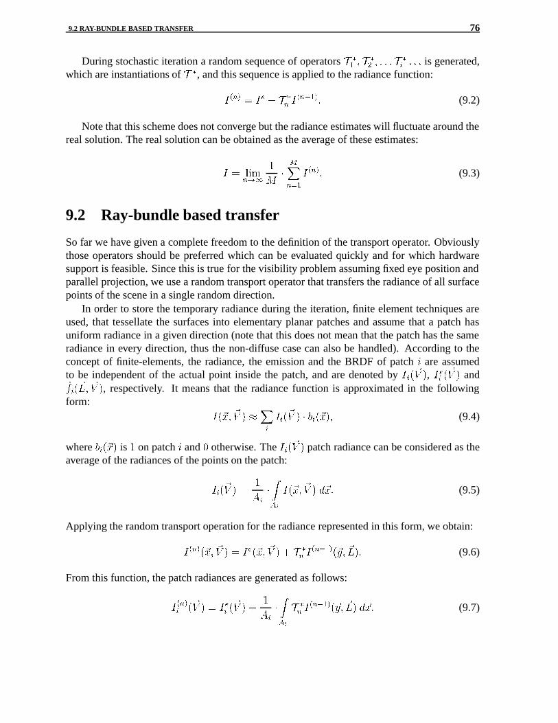
9.2 RAY-BUNDLE BASED TRANSFER 76

During stochastic iteration a random sequence of operators � �

� � � ��

� � � � is generated,which are instantiations of � �, and this sequence is applied to the radiance function:

��

� �� (9.2)

Note that this scheme does not converge but the radiance estimates will fluctuate around thereal solution. The real solution can be obtained as the average of these estimates:

� � ��

+�

��

�� (9.3)

9.2 Ray-bundle based transfer

So far we have given a complete freedom to the definition of the transport operator. Obviouslythose operators should be preferred which can be evaluated quickly and for which hardwaresupport is feasible. Since this is true for the visibility problem assuming fixed eye position andparallel projection, we use a random transport operator that transfers the radiance of all surfacepoints of the scene in a single random direction.

In order to store the temporary radiance during the iteration, finite element techniques areused, that tessellate the surfaces into elementary planar patches and assume that a patch hasuniform radiance in a given direction (note that this does not mean that the patch has the sameradiance in every direction, thus the non-diffuse case can also be handled). According to theconcept of finite-elements, the radiance, the emission and the BRDF of patch � are assumedto be independent of the actual point inside the patch, and are denoted by �� , �� and�� , respectively. It means that the radiance function is approximated in the followingform:

��

�� (�� (9.4)

where (�� is on patch � and � otherwise. The �� patch radiance can be considered as theaverage of the radiances of the points on the patch:

��

��

��

�� (9.5)

Applying the random transport operation for the radiance represented in this form, we obtain:

��

� �� (9.6)

From this function, the patch radiances are generated as follows:

��

��

��

� �

� �� (9.7)

9.2 RAY-BUNDLE BASED TRANSFER 77

Taking into account that in a given direction other patches are seen that have constant radi-ance, this integral can also be presented in closed form:

��

��

�� (9.8)

where �� expresses the projected area of patch that is visible from patch � in direction�. In the unoccluded case this is the intersection of the projections of patch � and patch ontoa plane perpendicular to �. If occlusion occurs, the projected areas of other patches that are inbetween patch � and patch should be subtracted as shown in Figure 9.1.

A

A j

iA(i,j,L)

Projection of

Projection of

AkProjection of Ak

Ai

A j

Projection plane

LL

Figure 9.1: Interpretation of ��

The resulting algorithm is quite simple. In a step of the stochastic iteration an image estimateis computed by reflecting the previously computed radiance estimate towards the eye, and a newdirection is found and this direction together with the previous direction are used to evaluate therandom transport operator. The complete algorithm — which requires just one variable for eachpatch �, the previous radiance �� — is summarized in the following algorithm:

Generate the first random global direction ��for each patch � do

�� = �� endforfor . � to + do // iteration cycles

Calculate the image estimate reflecting �� from �� towards the eye;Average the estimate with the Image;Generate random global direction ��for each patch � do

�� = �� = ��

�� endfor

endfor

9.3 CALCULATION OF THE RADIANCE TRANSPORT IN A SINGLE DIRECTION 78

9.3 Calculation of the radiance transport in a singledirection

To evaluate the transport operator, we need to know which patches are visible from a givenpatch, and then we have to weight the radiances of visible patches by the ratio of their visiblesizes and the size of the given patch.

This requires the solution of a global visibility problem, where the eye position visits allsurface points but the viewing direction is fixed to the selected random direction. This fixeddirection is called the transillumination direction (Figure 9.2).

At a given point of all global visibility algorithms the objects visible from the points ofa patch must be known (Figure 9.3). This information is stored in a data structure called thevisibility map . The visibility map can also be regarded as an image on the plane perpendicularto the transillumination direction. This plane is called the transillumination plane.

Transillumination direction

Transillumination plane

5

4

3

2

1

Figure 9.2: Global visibility algorithms

4 54 5

3

Image seen from patch 3 Image seen from patch 2

Figure 9.3: Scene as seen from two subsequent patches

9.4 HARDWARE IMPLEMENTATION OF THE PROPOSED RADIANCE TRANSFER ALGORITHM 79

Discrete algorithms, which decompose the transillumination plane to small pixels of size�$ , can solve the problem much faster. For discrete algorithms, the visibility map is simply arasterized image where each pixel can store either the index of the visible patch or the radianceof the visible point.

Discrete algorithms determine the image of the visible patches through a discretized windowassuming the eye to be on patch �, the window to be on the transillumination plane and the colorof patch to be if the patch is facing to patch � and to be � otherwise.

We use an extension of the z-buffer algorithm to identify the patches that see each otherthrough the pixels of the transillumination plane. The main difference from the original z-bufferalgorithm is that now a pixel should be capable to store a list of patch indices and z-values, notjust the values of the closest patch (Figure 9.4). The lists are sorted according to the z-values.The patches are rendered one after the other into the buffer using a modified z-buffer algorithmwhich keeps all visible points not just the nearest one. Traversing the generated lists the pairsof mutually visible points can be obtained. For each pair of points, the radiance transfer iscomputed and the transferred radiance is multiplied by the BRDF, resulting in the reflectedradiance.

1

2

3

Window

Transillumination buffer

Global direction

1 2 3

1 3

3

2

Figure 9.4: Organization of the transillumination buffer

9.4 Hardware implementation of the proposed radiancetransfer algorithm

The hardware of the radiance transfer algorithm is composed of two dependent stages, stageone (input interface and sorting the input data in memory) and stage two (output interface of thesorted data in memory). The input data is produced by the software and it is composed of arraysof patches with their related � values according to the screen position that these patches can be


seen. When the software initiates the data for the hardware, stage one fetches it and halts stagetwo until it finishes its operation of sorting the input data in memory according to the smallest �value of the patches that can be seen from the specific screen position. When stage one finishesits operation generates a signal to stage two to output the sorted data to the software.

The block scheme of this hardware is shown in Figure 9.5. This hardware runs according tothe data illustrated in Figure 9.4. The time sequence of stage one is shown in Figure 9.6 and itsVHDL description code is given by the following behavioral model:

ARCHITECTURE Behavior OF Control1 ISSIGNAL FP: ADDRESS := ("00........01"); -- Pointing to SCREEN_ADDRESS 1SIGNAL PR,PPR: ADDRESS; -- Pointer field is 24 bits wideSIGNAL ZR: DATA; -- DATA field is 24 bits wideSIGNAL Zero: DATA := (others => ’0’);BEGIN

PROCESSPROCEDURE Mem_Write (Addr: IN ADDRESS; d_w: IN DATA; Sel: in Sel_Type);PROCEDURE Mem_Read (Addr: IN ADDRESS; d_r: OUT DATA; Sel: in Sel_Type);

BEGINMem_Write(FP,Z,Sel_Z); Mem_Write(FP,I,Sel_I); Mem_Write(FP,Zero,Sel_P);Mem_Read(SCREEN_to_ADDRESS(S), PR, Sel_S);

-- SCREEN_ADDRESS 20 bits, extended to 24 bitsIF ( IsNull(PR) ) THEN

Mem_Write(SCREEN_to_ADDRESS(S), FP, Sel_S);ELSE -- Sel_Z selects Z_value field

PPR <= PR; -- Sel_S selects Screen fieldWHILE ( TRUE ) LOOP -- Sel_P selects pointer field

Mem_Read(PR,ZR,Sel_Z); -- Read z-value addressed by PRIF ( IsLessOrEq(Z,ZR) ) THEN -- Sel_I selects patches fieldEXIT;

END IF;PPR <= PR; Mem_Read(PR,PR,Sel_P);IF ( IsNull(PR) ) THEN -- If true, then end of storingEXIT;

END IF;END LOOP;

END IF;-- PPR is a pointer holding the previous value of a specific pointerIF ( IsNull(PR) ) THEN

Mem_Write(PPR,FP,Sel_P); -- Store the first addressELSEIF ( PR = PPR ) THEN

Mem_Write(SCREEN_to_ADDRESS(S),FP,Sel_S);Mem_Write(FP,PR,Sel_P);

ELSEMem_Write(PPR,FP,Sel_P); Mem_Write(FP,PR,Sel_P);

END IF;END IF;

FP <= Increment(FP); -- Free SCREEN pointerEND PROCESS;

END Behavior;


Z

Control1 Memory Conrol2

Start1

S

Ready

Din

Dout

A1Sel0

Sel1

Rd1

Wr1

Start2

CLK

0PReg.

Rd2

SPSel

StoreP

ClearSC

StepSCS counter

P Reg.

A2 Mpx

Stop2

Z PS I

Stage1Stage2

PValue

I

Stop1

<

<

10

00

01

11

Figure 9.5: Hardware implementation of radiance transfer algorithm

Figure 9.6: Stage one time sequence of the hardware implementation of radiance transfer algorithm

Chapter 10

Conclusions and summary of new results

In this thesis we proposed new image synthesis algorithms. These algorithms have solved thedrawbacks of linear interpolations and are comparable in image quality with the already known,sophisticated techniques but they have allowed simple hardware implementation. These algo-rithms cover the incremental cone-filtering lines, an alternative Phong shading using sphericalinterpolation, quadratic interpolation in Phong shading and texture mapping and ray-bundlebased global illumination. The main framework and the conclusions of these rendering algo-rithms are discussed in the following sections. The suggestions of the future research work isdeclared in Section 10.6.

10.1 General framework to compute simple functions on 2Dtriangles

In incremental rendering the geometric primitives are tessellated to triangles and line segmentsand are transformed and projected onto the screen coordinates. The projected triangles arefilled and the line segments are rasterized, i.e. those pixels are identified that approximate them,and pixel colors are computed simultaneously. Realizing that the pixel color can be a non-linear function of the pixel coordinates, a general framework and a supporting hardware weredeveloped to realize this filling operation together with the non-linear function computation.The computation is based on the so-called incremental concept, which means that a pixel valueis obtained as the increment value of the previous pixel. Since if the function is an � degreepolynomial, the increment is an �� degree polynomial, thus the computation of an � degreepolynomial can be traced back to an addition and to the evaluation of an �� degree polynomial.Using this idea recursively � parallel and fixed-point additions can compute the new value. Therequired accuracy was also investigated and we concluded that the required number of fractionalbits is proportional to the degree of the polynomial.

82

10.2 HARDWARE IMPLEMENTATION OF INCREMENTAL CONE-FILTERING LINES 83

10.2 Hardware implementation of incrementalcone-filtering lines

In order to reduce the jaggies of digital lines, the Gupta-Sproull algorithm applies conic filteringthat computes the conic volume above the intersection of the pixel and the base of the cone. Theresulting lines are of good quality, but the algorithm is computationally intensive. We proposethe transformation of this algorithm using the incremental concept that allows its hardwarerealization. In the new algorithm the distance between the line and the pixel center is evaluatedincrementally and the volume of the conic segment is obtained through a look-up table.

10.3 Hardware implementation of Phong shading usingspherical interpolation

Classical Phong shading interpolates the normal, view and light vectors inside the triangle andevaluates the rendering equation for each pixel in the triangle. The vector interpolation in-volves vector normalization, while the rendering equation requires dot product computationand exponentiation of scalar values. These operations are far too complex to be implemented inhardware. To attack the problem of vector normalization, we proposed the spherical interpola-tion of vectors [ASKH00], i.e. when the interpolation is done on the great arc of the surface of aunit sphere rather than on the line. Using quaternion algebra, the dot product of two sphericallyinterpolated vectors has been expressed as a simple cosine. Finally, the exponentiation of thecosine has been approximated by the ��! � � � (� function, where parameters ! and ( canbe determined from the original material parameters. We demonstrated that the approximationsneeded by the algorithm simplification do not degrade the visual quality of the rendered images.

10.4 Quadratic interpolation in rendering

Since rendering involves strongly non-linear operations, classical approaches using linear in-terpolation are inadequate for rendering high-quality images. To eliminate those artifacts wepropose a quadratic scheme [ASKHF00] for a function �:

�� '�� '�� '��

� � '�� '�� '��

In order to compute the unknown '�� '� parameters, the function to be interpolatedshould be evaluated at six representative points. In order to take into account the ease of com-putation and the elimination of visual inaccuracy called Mach banding, we propose the trianglevertices and the half points between the vertices for such representative points. We concludedthat this selection results in simple formulae and does not necessitate the solution of linearequations.

10.4 QUADRATIC INTERPOLATION IN RENDERING 84

10.4.1 Adaptive error control in quadratic interpolation

In order to control the error of the quadratic interpolation, the difference between the origi-nal function value and its approximation is compared and if it exceeds a certain threshold thetriangle is subdivided into � equivalent triangles.

10.4.2 Application of quadratic rendering for Phong shading and texturemapping

The idea of quadratic interpolation [ASKH�01a] was used to develop an alternative shadingalgorithm for Phong shading. The solution of the rendering equation is evaluated at six repre-sentative points and the color interpolation is done by the quadratic scheme in image space. Wedemonstrated that the quadratic interpolation is comparable to Phong shading in image quality.

Quadratic interpolation has also been used to solve the non-linearity problem of texturemapping [ASKH�01a] [ASKH�01b]. The texture coordinates are evaluated at six represen-tative points and the other pixels are approximated according to the quadratic formula. Wedemonstrated that the quadratic interpolation can avoid texture distortions.

Summarizing, the main problem of the original shading pipeline used by Phong shading(Figure 10.1) is that it involves complex operations such as lighting calculations and texturetransformations, which makes its direct hardware realization impossible.

Texture transform

Diffuselighting

Specularreflection

Texturememory

~~ Σ I * cos θ l

kd

Σ

u

v

X Y

Specular

DiffuseColor

1 lN,V,L . . . L vectorinterpolator

*

k s , n

l

Figure 10.1: Conventional rendering with Phong shading and texture mapping without interpolation

Traditionally, this problem is attacked by linear interpolation as shown by Figure 10.2,but the linear interpolation of the strongly non-linear functions degrades the image quality[SAFL99].


Texture transformat the vertices

Diffuse lighting at the vertices

Specular reflectionat the vertices

Linear texture interpolator

Linear diffuse lighting interpolator

Linear specular reflection interpolator

Texturememory

∼∼ Σ I * cos θ l

kd

Σ

u

v

X Y

Specular

DiffuseColor

*

l

Figure 10.2: Linear interpolation, i.e. Gouraud shading and linear texture mapping

In this thesis we proposed a new interpolation scheme (Figure 10.3) that uses appropriatelyselected quadratic functions which can be implemented in hardware and can be initialized with-out the computational burden of the Taylor’s series approach. Unlike previous techniques thenew method can simultaneously handle arbitrary number of light sources and arbitrary BRDFmodels.

Texturetransform at 6 points

Diffuse lighting at3 or 6 points

Specularreflection at 6 points

Quadratic texture coordinate interpolator

Linear or quadraticdiffuse lighting interpolator

Quadratic specular reflection interpolator

Texturememory

∼∼ Σ I * cos θ l

kd

Σ

u

v

X Y

Specular

DiffuseColor

*

l

Figure 10.3: Quadratic rendering

Figures 10.4, 10.5 and 10.6 show specular objects of more complex scenes with normal tes-sellation levels rendered with Gouraud shading, classical Phong shading and with the proposedquadratic rendering. Looking at these images we can conclude that the quadratic rendering isvisually superior to Gouraud shading and indistinguishable from classical Phong shading.


Figure 10.4: A shaded pawn with Gouraud (left), Phong (middle) and Quadratic (right)

Figure 10.5: A shaded and textured apple with Gouraud (left), Phong (middle) and Quadratic (right)

Figure 10.6: Coarsely tessellated, shaded, textured and specular tiger with Gouraud (left) Phong(middle) and quadratic (right)

10.5 HARDWARE IMPLEMENTATION OF GLOBAL ILLUMINATION 87

10.5 Hardware implementation of global illumination

The ray-bundle based stochastic iteration algorithm can render complex scenes according to theglobal illumination principles. In this thesis we presented a global visibility algorithm and itshardware realization, which can support its operation.

10.6 Suggestions of future research

We realized that during the last two decades there were enormous developments in the fieldof computer graphics software and hardware. The main objective of computer graphics is togenerate realistically looking images on a computer screen and as fast as possible. Taking intoaccount the computational burden associated with this process, real-time image synthesis ispossible only with either hardware support or with high-level parallelization. Recently, paral-lelization has become available on the low levels that are close to the hardware. The famouspixel shaders of the latest graphics cards delivered low level firmware programming featuresto the application developers. One possibility of the future research work could be the consid-eration of pixel shaders as an implementation framework for the proposed algorithms. On theother hand, there are many other computationally intensive methods of rendering, which canbe attacked by the simplification methods proposed in this thesis, including for example, so-phisticated texture filtering, and bump-, environment-, reflection- and displacement-mapping,volume visualization algorithms, etc. We believe that even these complex operations can beexecuted directly by the hardware in the future.

BIBLIOGRAPHY

[Abb95] A. M. Abbas. Programmable Logic Controller based Intel 80C196KB Microprocessor,M.Sc. Project. Faculty of Electrical Engineering and Informatics, Technical Universityof Budapest, Hungary, December, 1995.

[Abb98] A. M. Abbas. On 2D Line Scan Conversion. In Conference on The Latest Results in In-formation Technology, pages 50–57, Department of Control Engineering and InformationTechnology, Technical University of Budapest, Hungary, 1998.

[Abb01] A. M. Abbas. Photorealistic Images in Real-Time. Journal of Industrial Researches,Accepted for publication, Industrial Research Center, Tripoli Libya, June 2001.

[Ack96] H. Ackermann. Single chip hardware support for rasterization and texture mapping. Com-puters & Graphics, 20(4):503–514, 1996.

[Ash90] Peter J. Ashenden. The VHDL Cookbook. Department of Computer Science, Universityof Adelaide, South Australia, 1990.

[ASKH00] A. M. Abbas, L. Szirmay-Kalos, and T. Horvath. Hardware Implementation of PhongShading using Spherical Interpolation. Periodica Polytechnica, 44(3-4):283–301, 2000.

[ASKH�01a] A. M. Abbas, L. Szirmay-Kalos, T. Horvath, T. Foris, and Szijato G. Quadratic Inter-polation in Hardware Rendering. In Spring Conference on Computer Graphics, pages239–248, Budmerice, Slovakia, 25–28 April 2001.

[ASKH�01b] A. M. Abbas, L. Szirmay-Kalos, T. Horvath, T. Foris, and G. Szijarto. Quadratic Inter-polation in Hardware Phong Shading and Texture Mapping. In IEEE Computer SocietyPress in the Post-Proceedings of The 17th. Spring Conference on Computer Graphics,pages 181–188, Budmerice, Slovakia, 25–28 April 2001.

[ASKHF00] A. M. Abbas, L. Szirmay-Kalos, T. Horvath, and T. Foris. Quadratic Shading and itsHardware Interpolation. Machine GRAPHICS & VISION, 9(4):825–839, 2000.

[AVJ01] P. Arato, T. Visegrady, and I. Jankovits. High Level Synthesis of Pipelined Datapaths.JOHN WILEY & SONS, LTD, IIT, Budapest University of Technology and Economics,Hungary, 2001.

[BB99] V. Boyer and J. J. Bourdin. Fast Lines: a Span by Span Method. EUROGRAPHICS’99,18(3):C–377–C–384, 1999.

88

BIBLIOGRAPHY 89

[BERW97] K. Bennebroek, I. Ernst, H. Russeler, and O. Witting. Design principles of hardware-based Phong shading and bump-mapping. Computers & Graphics, 21(2):143–149, 1997.

[Bli77] J. F. Blinn. Models of Light Reflections for Computer Synthetized Pictures. In ComputerGraphics ( SIGGRAPH ’77 Proceedings), pages 192–198, 1977.

[BW86] G. Bishop and D. M. Weimar. Fast Phong Shading. Computer Graphics, 20(4):103–106,1986.

[Che97] Jim X. Chen. Multiple Segment Line Scan-conversion. COMPUTER GRAPHICS forum,16(5):257–268, 1997.

[Cla90] U. Claussen. On Reducing the Phong Shading Method. Computer & Graphics, 14(1):73–81, 1990.

[Cro81] F. C. Crow. A Comparison of Antialiasing Techniques. Computer Graphics and Appli-cations, 1(1):40–48, 1981.

[CT81] R. Cook and K. Torrance. A Reflectance Model for Computer Graphics. ComputerGraphics, 15(3), 1981.

[CW99] Jim X. Chen and Xusheng Wang. Approximate Line Scan-Conversion and Antialiasing.COMPUTER GRAPHICS forum, 18(1):69–78, 1999.

[DG96] D. Demirer and R. Grimsdale. Approximation techniques for high performance texturemapping. Computers and Graphics, 20(4):483–490, 1996.

[Duf79] T. Duff. Smoothly Shaded Rendering of Polyhedral Objects on Raster Displays. InComputer Graphics (SIGGRAPH ’79 Proceedings), 1979.

[DWS�88] M. Deering, S. Winner, B. Schediwy, C. Duffy, and Hunt N. The Triangle Processor andNormal Vector Shader: A VLSI System for High Performance Graphics. In ComputerGraphics (SIGGRAPH ’88 Proceedings), volume 22, pages 21–30, 1988.

[EWWL98] Jon P. Ewins, Marcus D. Waller, M. White, and Paul F. Lister. MIP-MAP Level Selec-tion for Texture Mapping. IEEE TRANSACTION ON VISULATION AND COMPUTERGRAPHICS, 4(4):317–329, 1998.

[FvDFH90] J. D. Foley, A. van Dam, S. K. Feiner, and J. F. Hughes. Computer Graphics: Principlesand Practice. Addison-Wesley, Reading, Mass., 1990.

[Gar75] P. L. Gardner. Modification of Bresenham’s Algorithm for Displays. IBM TechnicalDisclosure Bulletin, 18(5):1595–1596, 1975.

[GK92] R. L. Grimsdale and A. Kaufman. Advanced in computer graphics hardware V. Springer[etc.] 1992, Eurographics seminars, Berlin, 1992.

[Gou71] H. Gouraud. Computer Display of Curved Surfaces. ACM Transactions on Computers,C-20(6):623–629, 1971.

[GPC82] M. Gangnet, P. Perny, and P. Coueignoux. Perspective Mapping of Planar Textures. InEUROGRAPHICS ’82, pages 57–71, 1982.

BIBLIOGRAPHY 90

[GSS81] S. Gupta, R. Sproull, and I. Sutherland. Filtering Edges for Gray-Scale Displays. InComputer Graphics (SIGGRAPH ’81 Proceedings), pages 1–5, 1981.

[HBB01] A. Hast, T. Barrera, and E. Bengtsson. IMPROVED SHADING PERFORMANCE BYVECTOR NORMALIZATION. In Winter School of Computer Graphics’2001, volumeI–II, pages 344–351, Plzen, Czech Republic, 14–18 February 2001.

[Inc94] Model Technology Incorporated. VHDL Simulation for PCs Running Windows & Win-dows NT. Model Technology Incorporated, Beaverton OR 97008-7159 USA, 1994.

[Kaj86] J. T. Kajiya. The Rendering Equation. In Computer Graphics (SIGGRAPH ’86 Proceed-ings), pages 143–150, 1986.

[Kau93] A. Kaufman. Rendering, Visualization and Rasterization Hardware. EUROGRAPHICS,Department of Computer Science, State University of NY at Stony Brook, USA, 1993.

[KB89] A. A. M. Kuijk and E. H. Blake. Faster Phong Shading via Angular Interpolation. Com-puter Graphics Forum, (8):315–324, 1989.

[KSKA01] L. Kovacs, L. Szirmay-Kalos, and A. M. Abbas. Testing Global Illumination Methodswith Analytically Computable Scenes. In Winter School of Computer Graphics’01, vol-ume II, pages 419–426, Plzen, Czech Republic, 14–18 February 2001.

[KSKS96] G. KNITTEL, A. SCHILLING, A. KUGLER, and W. STRABER. HARDWARE FORSUPERIOR TEXTURE PERFORMANCE. Computer & Graphics, 20(4):475–481,1996.

[Kun93] Tosiyasu L. Kunii. Computer graphics: Theory and applications. Springer [etc.], Inter-Graphics, Tokyo, 1993.

[Kuz95] Yevgeny P. Kuzmin. Bresenham’s Lin generation Algoritm with Built-in Clipping. Com-puter Graphics Forum, 14(5):275–280, 1995.

[Lui94] Yong-Kui Lui. An All-integer Algorithm for Drawing Anti-aliased Straight Lines. COM-PUTER GRAPHICS forum, 13(4):219–221, 1994.

[Min41] M. Minnaert. The Reciprocity Principle in Lunar Photometry. Astrophysical Journal,93:403–410, 1941.

[MSKSA01] R. Martinez, L. Szirmay-Kalos, M. Sbert, and A. M. Abbas. Parallel Implementation ofStochastic Iteration Algorithms. In Winter School of Computer Graphics’01, volume II,pages 344–351, Plzen, Czech Republic, 14–18 February 2001.

[Nar95] Chandrasekhar Narayanaswami. Efficient Parallel Gouraud Shading and Linear Interpo-lation over Triangles. Computer Graphics Forum, 14(1):17–24, 1995.

[Per91] Douglas L. Perry. VHDL (Computer hardware description language). R. R. Donnelley& Sons Company, San Ramon, California, 1991.

[Pho75] B. T. Phong. Illumination for Computer Generated Images. Communications of the ACM,18:311–317, 1975.

BIBLIOGRAPHY 91

[RBX90] J. G. Rokne, W. Brian, and Wu. Xiaolin. Fast Line Scan-Conversion. ACM Transactionson Graphics, 9(4):376–388, 1990.

[RL98] Hassan K. Reghbati and Anson Y. C. Lee. Computer graphics hardware. IEEE ComputerSociety Press, USA, 1998.

[SAFL99] M. Segal, K. Akeley, C. Frazier, and J. Leech. The OpenGL graphics system: A specifi-cation. Technical Report (version 1.2.1), Silicon Graphics, Inc., 1999.

[SK95] L. Szirmay-Kalos. Theory of Three Dimensional Computer Graphics. Akademia Kiado,Budapest, 1995. http//www.iit.bme.hu/˜szirmay.

[SK99a] L. Szirmay-Kalos. Monte-Carlo Methods in Global Illumination. Institute of ComputerGraphics, Vienna University of Technology, Vienna, 1999.

[SK99b] L. Szirmay-Kalos. Stochastic iteration for non-diffuse global illumination. ComputerGraphics Forum (Eurographics’99), 18(3):233–244, 1999.

[SK00] L. Szirmay-Kalos. Photorealistic Image Synthesis with Ray-Bundles. HungarianAcademy of Sciences, D. Sc. Dissertation, Budapest, Hungary, 2000.

[SKM94] L. Szirmay-Kalos and G. Marton. On Hardware Implementation of Scan-conversion Al-gorithms. In 8th. Symp. on Microcomputer Appl., Budapest, Hungary, 1994.

[SKP98] L. Szirmay-Kalos and W. Purgathofer. Global ray-bundle tracing with hardware acceler-ation. In Rendering Techniques ’98, pages 247–258, 1998.

[SSW86] M. Samek, C. Slean, and H. Weghorst. Texture Mapping and Distortion in Digital Graph-ics. Visual Computer, 3:313–320, 1986.

[Str87] W. Strasser. Advanced in computer graphics I. Springer [etc.], Eurographics seminars,Eurographics workshop on graphics hardware, Lisbon, 1987.

[Wat89] A. Watt. Fundamentals of Three-dimensional Computer Graphics. Addison-Wesley,1989.

[WWD�95] M. White, M. D. Waller, G. J. Dunnett, P. F. Lister, and R. L. Grimsdale. Graphics ASICDesign Using VHDL. Computer & Graphics, 19(2):301–308, 1995.

[Xil01] Xilinx. Xilinx Synthesis Technology, Series Spartan-II FPGA Family Members. XILINX,2001.

[YR97] Chengfu Yao and Jon G. Rokne. Applying Rounding-Up Integral Linear Interpolationto the Scan-Conversion of Filled Polygons. Computer Graphics Forum, 16(2):101–106,1997.

AppendixMapping the RGB interpolators of the quadratic interpolation for the lower half

triangle on Xilinx Spartan2e device, FPGA Family Members, xc2s100e type

library IEEE;use IEEE.std_logic_$1164$.all;library unisim;use unisim.vcomponents.all;

package newpack issubtype sbyte is STD_LOGIC_VECTOR$(11$ downto $0$);subtype sword is STD_LOGIC_VECTOR($31$ downto $0$);subtype slong_word is STD_LOGIC_VECTOR($47$ downto $0$);end newpack;package body newpack isend newpack;

library IEEE;use IEEE.std_logic_$1164$.all;library unisim;use unisim.vcomponents.all;use work.newpack.all;entity IXYinterface is

port(StepIXsYR,StepIX1R,StepIY1R,InitIXsYR,InitIY1R, InitIY2R:out sword;StepIXsYG,StepIX1G,StepIY1G,InitIXsYG,InitIY1G, InitIY2G,StepIXsYB,StepIX1B,StepIY1B,InitIXsYB,InitIY1B, InitIY2B:out sword;Sel: in std_logic_vector(4 downto 0);iclk: in std_logic; idata: in sword);

end IXYinterface;

Architecture behaviour of IXYinterface isbeginregister_field_process:process(iclk) -- synchronous register load at rising edge of iclkbeginif iclk’event and iclk = ’1’ thencase Sel iswhen "00000" => StepIXsYR <= idata;when "00001" => StepIX1R <= idata;when "00010" => StepIY1R <= idata;

92

BIBLIOGRAPHY 93

when "00011" => InitIXsYR <= idata;when "00100" => InitIY1R <= idata;when "00101" => InitIY2R <= idata;when "00110" => StepIXsYG <= idata;when "00111" => StepIX1G <= idata;when "01000" => StepIY1G <= idata;when "01001" => InitIXsYG <= idata;when "01010" => InitIY1G <= idata;when "01011" => InitIY2G <= idata;when "01100" => StepIXsYB <= idata;when "01101" => StepIX1B <= idata;when "01110" => StepIY1B <= idata;when "01111" => InitIXsYB <= idata;when "10000" => InitIY1B <= idata;when "10001" => InitIY2B <= idata;when others => null;

end case;end if;end process;end behaviour;

library IEEE;use IEEE.std_logic_1164.all;library IEEE;use IEEE.std_logic_signed.all;library unisim;use unisim.vcomponents.all;use work.newpack.all;

ENTITY Interpolator IsPORT(clk,load_step: in STD_LOGIC; InitVal,StepVal: in sword;

OutVal: out sword);end Interpolator;

Architecture Behaviour of Interpolator issignal Adder_Out, Reg_Out: sword;beginregister_process:process(clk) -- sychronous load/step at rising edge of clkbegin

if clk’event and clk = ’1’ thenif load_step = ’1’ then

Reg_Out <= InitVal ;else

Reg_Out <= Adder_Out ;end if;

end if;end process;

BIBLIOGRAPHY 94

adder_process:process(Reg_Out,Stepval)begin

Adder_Out <= Reg_out + StepVal ;end process;

OutVal <= Reg_Out;end Behaviour;

library IEEE;use IEEE.std_logic_1164.all;library unisim;use unisim.vcomponents.all;use work.newpack.all;entity IXYgenerator is

port(clk,startX,startY:in STD_LOGIC;StepIXsYR,StepIX1R,StepIY1R,InitIXsYR,InitIY1R, InitIY2R:in sword;StepIXsYG,StepIX1G,StepIY1G,InitIXsYG,InitIY1G, InitIY2G,StepIXsYB,StepIX1B,StepIY1B,InitIXsYB,InitIY1B, InitIY2B:in sword;IXsYR,IX1R,IXYR,IXYG,IXYB:out sbyte);

end IXYgenerator;

architecture structure of IXYgenerator iscomponent interpolator

port(clk,load_step:in STD_LOGIC; InitVal,StepVal:in sword;OutVal:out sword);

end component;component Uinterpolator

port(clk,load_step:in STD_LOGIC; InitVal,StepVal:in sword;OutVal:out sword);

end component;

signal StepIXsYRs,InitIXsYRs, IXsYoutRs : sword;signal StepIX1Rs, IX1outRs, IX2outRs : sword;signal StepIY1Rs, InitIY1Rs, IY1outRs : sword;signal InitIY2Rs, IY2outRs: sword;signal StepIXsYGs, InitIXsYGs, IXsYoutGs : sword;signal StepIX1Gs, IX1outGs, IX2outGs : sword;signal StepIY1Gs, InitIY1Gs, IY1outGs : sword;signal InitIY2Gs, IY2outGs: sword;signal StepIXsYBs, InitIXsYBs, IXsYoutBs : sword;signal StepIX1Bs, IX1outBs, IX2outBs : sword;signal StepIY1Bs, InitIY1Bs, IY1outBs : sword;signal InitIY2Bs, IY2outBs: sword;signal dIX1clk, dIY1clk,dIY2clk,dIXsYclk,dIX2clk,dclk:STD_LOGIC;

begindclk <= clk;dIY2clk <= dclk and startX;dIY1clk <= dclk and startX;dIX2clk <= dclk ;dIX1clk <= dclk ;

BIBLIOGRAPHY 95

dIXsYclk <= dclk and startX;

IXsYRI:Uinterpolatorport map (dIXsYclk,startY,InitIXsYRs,StepIXsYRs,IXsYoutRs);

IX1RI:interpolatorport map (dIX1clk,startX,IXsYoutRs,StepIX1Rs,IX1outRs);

IX2RI:interpolatorport map (dIX2clk,startX,IY2outRs,IX1outRs,IX2outRs);

IY1RI:interpolatorport map (dIY1clk,starty,InitIY1Rs,StepIY1Rs,IY1outRs);

IY2RI:interpolatorport map (dIY2clk,starty,InitIY2Rs,IY1outRs,IY2outRs);

IXsYGI:Uinterpolatorport map (dIXsYclk,starty,InitIXsYGs,StepIXsYGs,IXsYoutGs);

IX1GI:interpolatorport map (dIX1clk,startX,IXsYoutGs,StepIX1Gs,IX1outGs);

IX2GI:interpolatorport map (dIX2clk,startX,IY2outGs,IX1outGs,IX2outGs);

IY1GI:interpolatorport map (dIY1clk,starty,InitIY1Gs,StepIY1Gs,IY1outGs);

IY2GI:interpolatorport map (dIY2clk,starty,InitIY2Gs,IY1outGs,IY2outGs);

IXsYBI:Uinterpolatorport map (dIXsYclk,starty,InitIXsYBs,StepIXsYBs,IXsYoutBs);

IX1BI:interpolatorport map (dIX1clk,startX,IXsYoutBs,StepIX1Bs,IX1outBs);

IX2BI:interpolatorport map (dIX2clk,startX,IY2outBs,IX1outBs,IX2outBs);

IY1BI:interpolatorport map (dIY1clk,starty,InitIY1Bs,StepIY1Bs,IY1outBs);

IY2BI:interpolatorport map (dIY2clk,starty,InitIY2Bs,IY1outBs,IY2outBs);

StepIXsYRs <= StepIXsYR;InitIXsYRs <= InitIXsYR;StepIX1Rs <= StepIX1R;StepIY1Rs <= StepIY1R;InitIY1Rs <= InitIY1RInitIY2Rs <= InitIY2R;IXsYR<= IXsYoutRs(31 downto 20);IX1R <= IX1outRs(31 downto 20);IXYR <= IX2outRs(31 downto 20);StepIXsYGs <= StepIXsYG;InitIXsYGs <= InitIXsYG;StepIX1Gs <= StepIX1G;StepIY1Gs <= StepIY1G;InitIY1Gs <= InitIY1G;InitIY2Gs <= InitIY2G;IXYG <= IX2outGs(31 downto 20);StepIXsYBs <= StepIXsYB;InitIXsYBs <= InitIXsYB;StepIX1Bs <= StepIX1B;

BIBLIOGRAPHY 96

StepIY1Bs <= StepIY1B;InitIY1Bs <= InitIY1B;InitIY2Bs <= InitIY2B;IXYB <= IX2outBs(31 downto 20);end structure;

library IEEE;use IEEE.std_logic_1164.all;library IEEE;use IEEE.std_logic_signed.all;library unisim;use unisim.vcomponents.all;use work.newpack.all;

ENTITY UInterpolator IsPORT(clk,load_step: in STD_LOGIC; InitVal,StepVal: in sword;

OutVal: out sword);end UInterpolator;

Architecture Behaviour of UInterpolator issignal Adder_Out, Reg_Out: sword;beginregister_process:process(clk,load_step, InitVal)begin

if load_step = ’1’ thenReg_Out <= InitVal ;elseif clk’event and clk = ’1’ then

Reg_Out <= Adder_Out ;end if;

end if;end process;

adder_process:process(Reg_Out,Stepval)beginAdder_Out <= Reg_Out + Stepval ;end process;

OutVal <= Reg_Out;end Behaviour;

library IEEE;use IEEE.std_logic_1164.all;library unisim;use unisim.vcomponents.all;

BIBLIOGRAPHY 97

use work.newpack.all;entity conn isport(Sel: in std_logic_vector(4 downto 0); iclk: in std_logic;

idata: in sword; clk,startX,startY:in STD_LOGIC;IXsYRb,IX1Rb,IXYRb,IXYGb,IXYBb:out sbyte);

end conn;

architecture structure of conn iscomponent IXYinterfaceport(StepIXsYR,StepIX1R,StepIY1R,InitIXsYR,InitIY1R, InitIY2R:out sword;

StepIXsYG,StepIX1G,StepIY1G,InitIXsYG,InitIY1G, InitIY2G,StepIXsYB,StepIX1B,StepIY1B,InitIXsYB,InitIY1B, InitIY2B:out sword;Sel: in std_logic_vector(4 downto 0);iclk: in std_logic; idata: in sword);

end component;

component IXYgeneratorport(clk,startX,startY:in STD_LOGIC;

StepIXsYR,StepIX1R,StepIY1R,InitIXsYR,InitIY1R, InitIY2R:in sword;StepIXsYG,StepIX1G,StepIY1G,InitIXsYG,InitIY1G, InitIY2G,StepIXsYB,StepIX1B,StepIY1B,InitIXsYB,InitIY1B, InitIY2B:in sword;IXsYR,IX1R,IXYR,IXYG,IXYB:out sbyte);

end component;

signal StepIXsYR,StepIX1R,StepIY1R,InitIXsYR,InitIY1R, InitIY2R,StepIXsYG,StepIX1G,StepIY1G,InitIXsYG,InitIY1G, InitIY2G,StepIXsYB,StepIX1B,StepIY1B,InitIXsYB,InitIY1B, InitIY2B:sword;

signal IXsYR,IX1R,IXYR,IXYG,IXYB: sbyte;beginIXsYRb <= IXsYR;IX1Rb <= IX1R;IXYRb <= IXYR;IXYGb <= IXYG;IXYBb <= IXYB;

Generator_hw:IXYgenerator port map (clk,startX,startY,

StepIXsYR,StepIX1R,StepIY1R,InitIXsYR,InitIY1R, InitIY2R,StepIXsYG,StepIX1G,StepIY1G,InitIXsYG,InitIY1G, InitIY2G,StepIXsYB,StepIX1B,StepIY1B,InitIXsYB,InitIY1B, InitIY2B,IXsYR,IX1R,IXYR,IXYG,IXYB);

Interface_hw:IXYinterface port map (StepIXsYR,StepIX1R,StepIY1R,InitIXsYR,InitIY1R, InitIY2R,StepIXsYG,StepIX1G,StepIY1G,InitIXsYG,InitIY1G, InitIY2G,StepIXsYB,StepIX1B,StepIY1B,InitIXsYB,InitIY1B, InitIY2B, Sel, iclk, idata);

end structure;

BIBLIOGRAPHY 98

Design Information------------------Target Device : x2s100eTarget Package : ft256Target Speed : -6

Design Summary--------------

Number of Slices: 883 out of 1,200 73%Number of Slices containing

unrelated logic: 0 out of 883 0%Number of Slice Flip Flops: 1,056 out of 2,400 44%Number of 4 input LUTs: 1,183 out of 2,400 49%Number of bonded IOBs: 99 out of 178 55%Number of GCLKs: 2 out of 4 50%Number of GCLKIOBs: 2 out of 4 50%

Total equivalent gate count for design: 18,336Additional JTAG gate count for IOBs: 4,848

---- Target ParametersTarget Device : xc2s100e-ft256-6Target Technology : spartan2e

---- Source OptionsAutomatic FSM Extraction : YESFSM Encoding Algorithm : AutoFSM Flip-Flop Type : DMux Extraction : YESResource Sharing : YESComplex Clock Enable Extraction : YESROM Extraction : YesRAM Extraction : YesRAM Style : AutoMux Style : AutoDecoder Extraction : YESPriority Encoder Extraction : YESShift Register Extraction : YESLogical Shifter Extraction : YESXOR Collapsing : YESAutomatic Register Balancing : No

---- Target OptionsAdd IO Buffers : YESEquivalent register Removal : YESAdd Generic Clock Buffer(BUFG) : 4Global Maximum Fanout : 100Register Duplication : YESMove First FlipFlop Stage : YESMove Last FlipFlop Stage : YESSlice Packing : YESPack IO Registers into IOBs : autoSpeed Grade : 6

BIBLIOGRAPHY 99

---- General OptionsOptimization Criterion : SpeedOptimization Effort : 1Check Attribute Syntax : YESKeep Hierarchy : NoGlobal Optimization : AllClockNetsWrite Timing Constraints : No========================================================HDL Synthesis Report FPGA Macro Statistics# Registers : 33

32-bit register : 33# Multiplexers : 15

2-to-1 multiplexer : 15# Adders/Subtractors : 15

32-bit adder : 15========================================================Design Statistics# IOs : 101

Cell Usage :# BELS : 2114# BUF : 5# GND : 1# LUT2 : 212# LUT2_D : 15# LUT2_L : 450# LUT3 : 35# LUT3_L : 465# LUT4 : 1# MUXCY : 465# XORCY : 465# FlipFlops/Latches : 1056# FD : 384# FDCP : 96# FDE : 576# Clock Buffers : 2# BUFGP : 2# IO Buffers : 99# IBUF : 39# OBUF : 60==========================================================Timing Summary:---------------

Minimum period: 7.148ns (Maximum Frequency: 139.899MHz)Minimum input arrival time before clock: 14.470nsMaximum output required time after clock: 6.778ns

TRANSFORMATION OF RENDERING ALGORITHMS FOR …sirkan.iit.bme.hu/~szirmay/abbas.pdfTRANSFORMATION OF...

Documents

Transcript of TRANSFORMATION OF RENDERING ALGORITHMS FOR …sirkan.iit.bme.hu/~szirmay/abbas.pdfTRANSFORMATION OF...