Transform Based and Search Aware Text Compression Schemes and Compressed Domain Text Retrieval Nan...
123
Transform Based and Search Aware Text Compression Schemes and Compressed Domain Text Retrieval Nan Zhang PhD Candidate School of Computer Science University of Central Florida Spring, 2005
-
Upload
leona-brown -
Category
Documents
-
view
232 -
download
0
Transcript of Transform Based and Search Aware Text Compression Schemes and Compressed Domain Text Retrieval Nan...

Transform Based and Search Aware Text Compression
Schemes and Compressed Domain Text Retrieval
Nan ZhangPhD Candidate
School of Computer ScienceUniversity of Central Florida
Spring, 2005

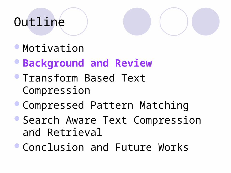
Outline
MotivationBackground and ReviewTransform Based Text CompressionCompressed Pattern MatchingSearch Aware Text Compression and
Retrieval Conclusion and Future Works

Motivation
Decrease storage requirementsEffective use of communication bandwidthIncreased data securityMultimedia data on information
superhighwayGrowing number of “killer” applications.Find information from the “sleeping” files.
Growth of Data
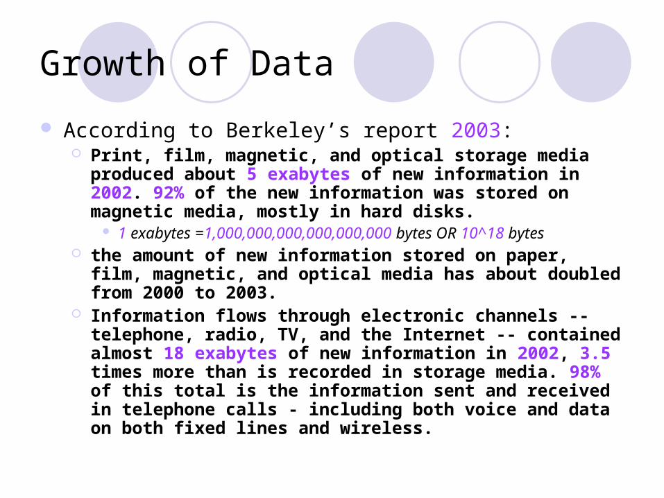
According to Berkeley’s report 2003: Print, film, magnetic, and optical storage media produced
about 5 exabytes of new information in 2002. 92% of the new information was stored on magnetic media, mostly in hard disks.
1 exabytes =1,000,000,000,000,000,000 bytes OR 10^18 bytes the amount of new information stored on paper, film,
magnetic, and optical media has about doubled from 2000 to 2003.
Information flows through electronic channels -- telephone, radio, TV, and the Internet -- contained almost 18 exabytes of new information in 2002, 3.5 times more than is recorded in storage media. 98% of this total is the information sent and received in telephone calls - including both voice and data on both fixed lines and wireless.

Brief History of Data Compression
1838: Morse Code: using shorter codes for more commonly used letters.
Late 1940’s: born of Information Theory. 1948: Claude Shannon and Robert Fano using probabilities of blocks. 1953: Huffman Coding. 1987: Arithmetic Coding.
1977, 1978 (LZ77, LZ78): Abraham Lempel and Jacob Ziv they assigned codewords to repeating patterns in the text.
1984 (LZW): Terry Welch, from LZ78. 1987 (DMC): Cormack and Horspool, Dynamic Markov Model. 1989 (PPM): Cleary and Witten. 1994 (BWT): Burrows and Wheeler, block sorting. Others: Run-Length Coding (RLE), Move-to-Front (MTF), Vector
Quantization (VQ), Discrete Cosine Transform (DCT), Wavelet methods, etc.

Our Contribution (I)
Star family compression algorithms: A reversible transformation that can be applied to a
source text that improves existing algorithm's ability to compress.
We use a static dictionary to convert the English words into predefined symbol sequences.
Create additional context information that is superior to the original text.
Use ternary tree data structure to expedite the transformation.

Our Contribution (II)
Exact and approximate pattern matching in Burrows-Wheeler transformed (BWT) text. Compressed Pattern Matching (CPM) domain. Extract auxiliary arrays to facilitate matching. K-mismatching. K-approximate matching. CPM up to MTF stage in BWT based
compression.
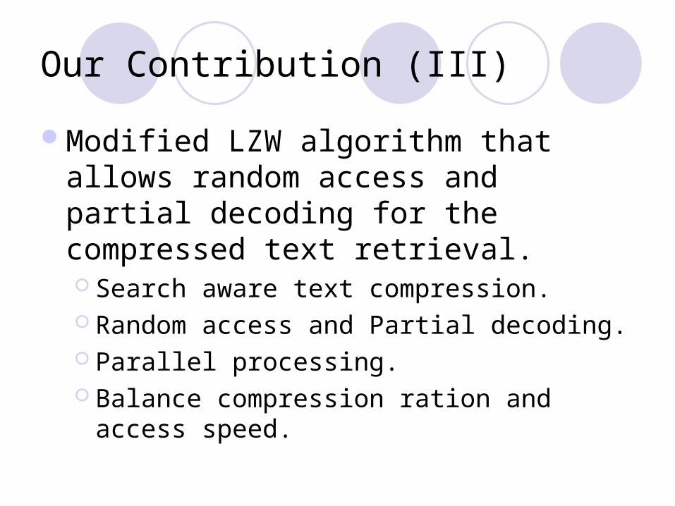
Our Contribution (III)
Modified LZW algorithm that allows random access and partial decoding for the compressed text retrieval. Search aware text compression. Random access and Partial decoding. Parallel processing. Balance compression ration and access speed.
Outline
MotivationBackground and ReviewTransform Based Text CompressionCompressed Pattern MatchingSearch Aware Text Compression and
Retrieval Conclusion and Future Works
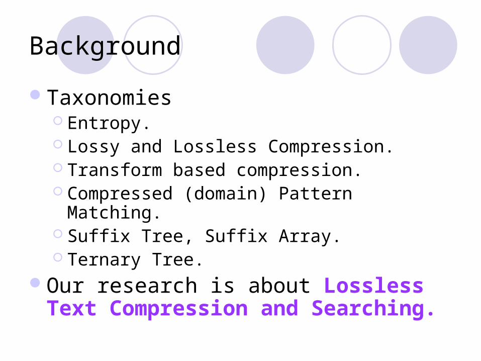
Background
Taxonomies Entropy. Lossy and Lossless Compression. Transform based compression. Compressed (domain) Pattern Matching. Suffix Tree, Suffix Array. Ternary Tree.
Our research is about Lossless Text Compression and Searching.

Lossless Text Compression
Basic techniques Run-Length Move-to-Front Distance Coding
Statistical methods: variable-sized codes based on the statistics of the symbols or group of symbols. Huffman, Arithmetic PPM (PPMC, PPMD, PPMD+, PPMZ …)
Dictionary methods: encode a sequence of symbols with another token LZ (LZ77, LZ78, LZW, LZH …)
Transform base methods: BWT
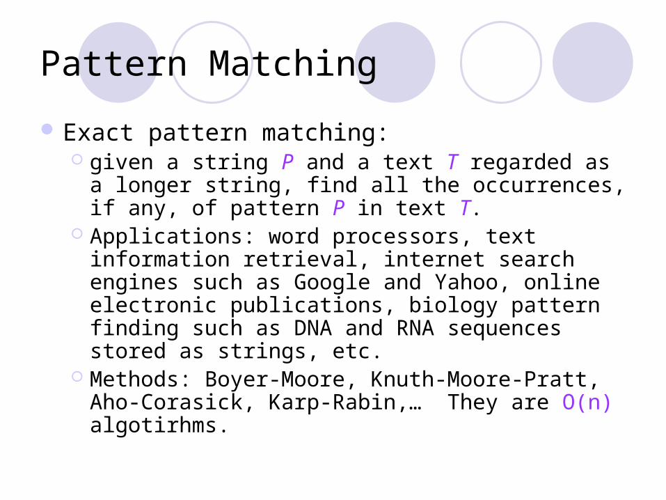
Pattern Matching
Exact pattern matching: given a string P and a text T regarded as a longer
string, find all the occurrences, if any, of pattern P in text T.
Applications: word processors, text information retrieval, internet search engines such as Google and Yahoo, online electronic publications, biology pattern finding such as DNA and RNA sequences stored as strings, etc.
Methods: Boyer-Moore, Knuth-Moore-Pratt, Aho-Corasick, Karp-Rabin,… They are O(n) algotirhms.

Pattern Matching
Subproblems: suffix tree, suffix array, longest common
ancestor, longest common substring When we search in the compressed text, we will
try to build such structures on the fly by (partially) decomposing the compressed text

Approximate Pattern Matching
Looking for simliar patterns involves: definition of distance/similarity between the
patterns the degree of error allowed
Subproblems: dynamic programming, longest common sequences
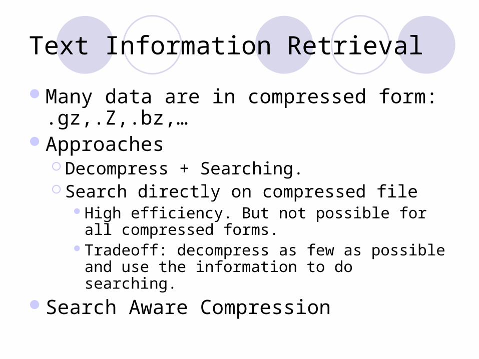
Text Information Retrieval
Many data are in compressed form: .gz,.Z,.bz,…
Approaches Decompress + Searching. Search directly on compressed file
High efficiency. But not possible for all compressed forms.
Tradeoff: decompress as few as possible and use the information to do searching.
Search Aware Compression

Outline
MotivationBackground and ReviewTransform Based Text CompressionCompressed Pattern MatchingSearch Aware Text Compression and
Retrieval Conclusion and Future Works

Data Compression
Lossless Compression Text Compression (gzip, compress) Digitized Audio Compression (PCM, DPCM) Digitized Image Compression (GIF, TIFF)
Lossy Compression Text Compression (Summary) Digitized Audio Compression (RM, MP3) Digitized Image Compression (JPEG, MPEG)
We focus on Lossless Text Compression

Model Data Compression
Coding
Source Messages, M Codeword, C
(alphabet ) (alphabet )
Properties
•Distinct
•Uniquely Decipherable (Prefix)
•Instantaneously Decodable
•Minimal Prefix
f

Data Compression Stages
Preliminary compression steps. (LIPT, BWT)
Organization by context. (MTF,DC)
Probability estimation. (PPM, DMC)
Length-reducing code. (Huffman, Arithmetic)

Information Theory Basics
Given a source S with an alphabet that generates a sequence
First order entropy:
Entropy of the source:
where
and is a sequence of length n from the source
m
i
iPiPSH1
)(log)()(
m,,2,1 ,,2,1 XX
nn
Gn
SH1
lim)(
mi
i
mi
i
mi
innnnn
n
n
iXiXiXPiXiXiXPG1
1
2
21 1 1,22,11,22,11 )(log)(
nXXX 21,

Text Compression Algorithms Data Compression
It is easier to compute the first order entropy by using the frequency of the occurrences of the symbols as the estimation of the probability.
When higher order is considered, there might exist the correlation between the subsequences.
The order can be considered the length of the subsequences. The compression algorithm aims to reach the bound given by the
entropy. Difficulty: we do not know the general entropy of a source
because the order can be as high as infinity and that the equation of computing the entropy does not give any hint of how to actually reach that entropy bound.

First Order Entropy Coder Data Compression
Huffman Coding Word Huffman Canonical Huffman
Arithmetic Coding Can approach to arbitrary precision

Dictionary Models Data Compression
LZ family LZ77: Match history patterns with a finite
window LZ78:Build explicit dictionary LZW: Variation of LZ78 (removing the last
element)
Good compression and fast: gzip, unix Compress,etc.

Statistical Models Data Compression
PPM (Predict by Pattern Matching) family with different zero-frequency estimation methods: PPMC PPMD …
DMC (Dynamic Markov Compression)
Mixture Models Data Compression
Burrows-Wheeler Transform It is not a actual “compression” method. The output of BWT is good for entropy coder
after MTF (move-to-front) algorithm. Can be used for compressed searching.

Star Transform Model
Perform a lossless, reversible transformation to a source file prior to applying an existing compression algorithm
The basic philosophy of the compression algorithm is to transform the text into some intermediate form, which can be compressed with better efficiency.

Star Transform Model
Original text:This is a test.
Transform encoding
Transformed text:***a^ ** * ***b.
Data compression
Compressed text:(binary code)
Data decompressionOriginal text:This is a test.
Transform decoding
Transformed text:***a^ ** * ***b.

Dictionary
All the transforms use an English language dictionary D that has about 60,000 words (current dictionary) 500Kbytes.
Shared by both compression and decompression ends. This English dictionary D is partitioned into disjoint dictionaries
Di, each containing words of length i, where i = 1,2…n. Each dictionary Di is partially sorted according to the
frequency of words in the English language. A mapping is used to generate the encoding for all words in
each dictionary Di. Di[j] denotes the jth word in dictionary Di. If the word in the input text is not in the English dictionary (viz.
a new word in the lexicon) it will be passed to the transformed text unaltered. Special characters and alphabet capitalization is also handled by escape character.

Star Family Transforms
*-Encoding replaces each character in the input word by a special placeholder character ‘*’ and retains at most two characters from the original word. It preserves the length of the original word in the
encoding. e.g. the one letter word ‘a’ will be encoded as ‘*’ , ‘am’
will be encoded as ‘*a’ , the word ‘there’ will be encoded as ‘*****’, and ‘which’ will be encoded as ‘a*****’.

Star Family Transforms
LPT transform encodes the input word as *pc1c2c3 where c1c2c3 give the dictionary offset of the corresponding word (c1 cycles through z-a, c2 cycles through A-Z, c3
cycles through a-z), and p is the padding sequence (suffix of the string ‘…nopqrstuvw’) to equalize the length of encoded and original input word. The number of dictionary offset characters(at the end) is
fixed for all words. e.g. the first word of length nine in the original dictionary
will be encoded as *stuvwzAa

Star Family Transforms
RLPT also encodes the input word as *pc1c2c3 but uses
the reverse string for p i.e. suffix of the string ‘wvutsrqpon…’ .
e.g. the first word of length nine in the original dictionary will be encoded as *wvutszAa

Star Family Transforms
SCLPT transform does not preserve the original length of the input word.
Encodes the input word as *pc1c2c3 but discards all the characters except the first one in the LPT padding sequence p. This character is used to determine the sequence of characters that follow up to the last character ‘w’ in LPT. e.g. the first word of length nine in the original dictionary
will be encoded as *szAa.

Star Family Transforms
LIPT- Length Index Preserving Transform introduces the idea of using a character denoting the length of the original word. It is given by *cl[c1][c2][c3] where cl is an alphabet [a-z] denoting the length of input word ( a denotes length of 1, b length of 2,…, z length of 26, A 27…., Z denotes 52). The number of Last characters giving the dictionary offset (with respect to the start of each length block) is variable and not fixed as in last three transforms. Each of c1,c2,c3 cycles through [a-zA-z]. e.g first word of length ten in the original dictionary will be
encoded as *j, second word as *ja,fifty fourth as *jaa, 2758th word will be encoded as *jaaa .

Star Family Transforms
Original Text (83 bytes):
It is truly a magnificent piece of work.
constitutionalizing
internationalizations
*- (84 bytes):
r*~ q* v*D** * OC********* Vl*** y* Q***.
b******************
*********************

Star Transforms Examples
RLPT (84 bytes):r*~ q* *wtbE * *wvutsrqwzD *wvaM y* *zbR.*wvutsrqponmlkjizaC
*wvutsrqponmlkjihgzaA SCLPT (48 bytes):
*s~ *r *wtbE * *qwzD *wvaM *z *zbR.*izaC*gzaA
LIPT (44 bytes):*br~ *bq *eazD *a *kYC *eZl *by *dQ.*sb*u

Test Corpus Data Compression
Calgary Canterbury Textfiles (from Gutenberg)FileNames Actual Sizes FileNames Actual Sizes FileNames Actual Sizesbib 111261 alice29.txt 152089 1musk10.txt 1344739book1 768771 asyoulik.txt 125179 anne11.txt 586960book2 610856 cp.html 24603 world95.txt 2988578news 377109 fields.c 11150paper1 53161 grammar.lsp 3721paper2 82199 lcet10.txt 426754paper3 46526 plrabn12.txt 481861paper4 13286 xargs.1 4227paper5 11954 bible.txt 4047392paper6 38105 kjv.gutenberg 4846137progc 39611 world192.txt 2473400progl 71646progp 49379trans 93695

Results
Bzip2 (Average
BPC
PPMD (order 5) (Average
BPC)
Gzip –9 (Average
BPC)
Original
2.28 2.14 2.70
LIPT 2.16 2.04 2.52
% improvement
5.3% 4.5% 6.7%

Dictionary Overhead
The size of English dictionary is 500kb uncompressed and 197KB when compressed with Bzip2.
Let the uncompressed size of the data to be transmitted be F and the uncompressed dictionary size be D. Then for Bzip2 with LIPT :
F 2.16 + D 2.28 F 2.28, which gives F 9.5 MB. To break even the overhead associated with dictionary, transmission of
9.5MB data has to be achieved. If the normal file size for a transmission is 1 MB then the dictionary overhead will break even after about 9.5 transmissions. All the transmission above this number contributes towards gain achieved by LIPT.
Similarly for PPMD with LIPT, F 10.87 MB. With increasing dictionary size, this threshold will go up, but in a scenario
where thousands of files are transmitted, the amortized cost will be negligible.

Fast Implementation
Hash table Binary tree Digital search tries Ternary search trees
Searching for a string of length k in a ternary search tree with nstrings will require at most O(log n+k) CHAR comparisons

Timing Performance -- Compared with LIPT
Encoding
Decoding
76.3%
84.9%

Timing Performance -- Compared with Backend Compressor
28.1%
Bzip2 -9
Enc
odin
gD
ecod
ing
50.4%
Gzip -9
21.2%
PPMD (k=5)
Some minimal increase18.6%

Outline
MotivationBackground and ReviewTransform Based Text CompressionCompressed Pattern MatchingSearch Aware Text Compression and
Retrieval Conclusion and Future Works

Pattern Matching
Pattern Matching Why?
Searching in DNA sequence, Information retrieval…
How? Naïve Algorithm Smarter Algorithms:
• Knuth-Moore-Pratt• Boyer-Moore• Suffix tree• Suffix array• …

Pattern Matching Algorithms
Naïve: O(mn) |P|=n |T|=m
BM: O(n+m) KMP: O(n+m) Aho-Corasick: O(n+m) Shift-And: O(mn) bit operations Suffix tree: O(m+n)
Space resuction: Suffix array. Can use binary search

Suffix Tree Pattern Matching
The label of a path from the root that ends at a node is the concatenation, in order, of the substrings labeling the edges of that path. The path-label of a node is the label of the path from the root of T to that node.
For any node v in a suffix tree, the string-depth of v is the number of characters in v’s label.
A path that ends in the middle of an edge (u,v) splits the label on (u,v) at a designated point. Define the label of such a path as the label of u concatenated with the characters on edge (u,v) down to the designated split point.An implicit suffix tree for string S is a tree obtained from the suffix tree for S$ by removing every copy of the terminal symbol $ from the edge labels of the tree, then removing any edge that has no label, and then removing any node that does not have at least two children.We denote the implicit suffix tree of the string S[1..i] by Ii,for i from 1 to m.

Suffix Array Pattern Matching
Definition: Given an m-character string T, a suffix array of T, called Pos, is an array of the integers in the range 1 to m, specifying the lexicographic order of the m suffixes of string T.
Suffix array can be obtained in linear time by performing a “lexical” depth-first traversal of T.

Approximate Pattern Matching Pattern Matching
Edit distance problem K-mismatch problem K-approximate problem

Compressed Pattern Matching
Motivation: When the sheer volume of data provided to users, they
are increasingly in compressed format: .gz, .tar.gz, etc. Storage & transmission Information retrieval Speed

Compressed Pattern Matching
DefinitionGiven T a text string, P a pattern, and Z the compressed
representation of T, locate the occurrences of P in T with minimal (or no) decompression of Z.
Approach Decompress + Searching Search directly on compressed file
High efficiency. But not possible for all compressed forms Tradeoff: decompress as few as possible and use the
information to do searching.

Compressed Pattern Matching
Amir et.al. search a pattern in LZ-77 compressed text on
time, where m=|P|, u=|T|, and n=|Z|. Bunke et.al. search for patterns in run-length encoded
files in time. Where is the length of pattern when it is compressed.
Moura.et. al. proposed algorithms on Huffman-encoded files.
Special compressed schemes facilitate latter pattern Matching (Manber, Shibata, Kida, etc).
))/(log( 2 mnunO
)( cumO cm
)( nmnO

Compressed Pattern Matching
Little has been done on searching directly on text compressed with the Burrows-Wheeler Transform (BWT).
Compression Ratio: BWT is significantly superior to the popular LZ-based methods such as gzip and compress, and only second to PPM.
Running Time: much faster than PPM, but comparable with LZ-based algorithms
Exact Matching in BWT Text
BWT performs a permutation of the characters in the text, such that characters in lexically similar contexts will be near to each other.

Burrows-Wheeler Transform
Forward Transform Given an input text ,
1. Form u permutations of T by cyclic rotations of characters in T, forming a uxu matrix M’, with each row representing one permutation of T.
2. Sort the rows of M’ lexicographically to form another matrix M, including T as one of rows.
3. Record L, the last column of M, and id, the row number where T is in M.
4. Output of BWT is (L, id).
utttT 21
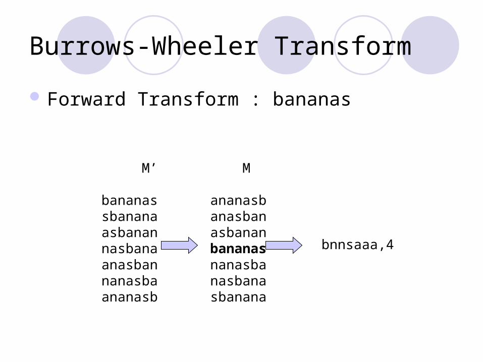
Burrows-Wheeler Transform
Forward Transform : bananas
M’
bananassbananaasbanannasbanaanasbannanasbaananasb
M
ananasbanasbanasbananbananasnanasbanasbanasbanana
bnnsaaa,4

Burrows-Wheeler Transform
Inverse Transform: Given only the (L,id) pair
1. Sort L to produce F, the array of first characters
2. Compute V, provides 1-1 mapping between the elements of L and F. F[V [j]]=L[j].
3. Generate original text T, the symbol L[j] cyclically precedes the symbol F[j] in T, that is, L[V [j]] cyclically precedes the symbol L[j] in T.

Burrows-Wheeler Transform
F L a ba na nb s id =4 n an as a
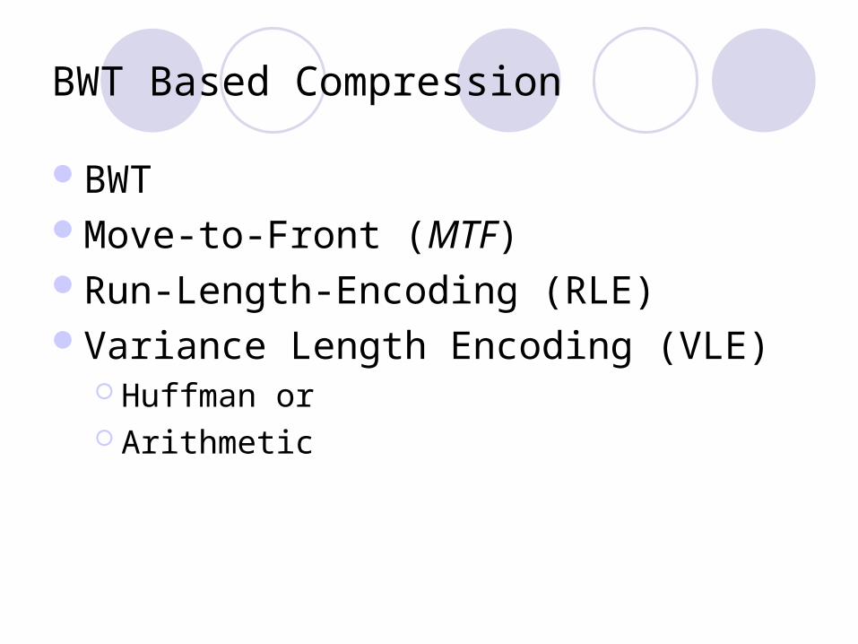
BWT Based Compression
BWTMove-to-Front (MTF)Run-Length-Encoding (RLE)Variance Length Encoding (VLE)
Huffman or Arithmetic

Motivations
BWT provides a lexicographic ordering of the input text as part of its inverse transform process.
It maybe possible to perform an initial match on a symbol and its context, and then decode only that part of text.
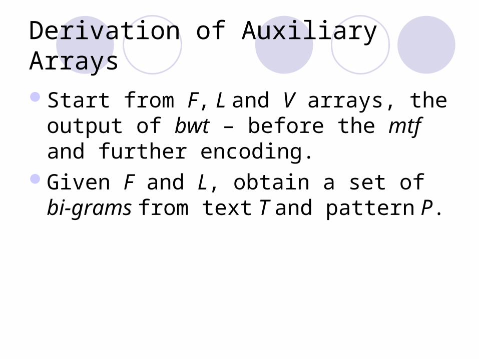
Derivation of Auxiliary Arrays
Start from F, L and V arrays, the output of bwt – before the mtf and further encoding.
Given F and L, obtain a set of bi-grams from text T and pattern P.

Derivation of Auxiliary Arrays
T=abraca:F …. L V FS FST …… M
a c 5 aa aab aabrac
a a 1 ab abr abraca
a r 6 ac aca acaabr
b a 2 br bra bracaa
c a 3 ca caa caabra
r b 4 ra rac racaab

Derivation of Auxiliary Arrays
Generating q-grams from BWT outputGrams(F,L,V,q) F(1-gram) = F;
for x = 2 to q dofor i = 1 to u do
F(x-gram)[V(i)] := L[I]*F((x-1)-gram)[i]; end; end;* Denotes concatenation. If q=2, the result will be the
sorted bi-grams;

Derivation of Auxiliary Arrays
T=abraca:F …. L V FS FST …… M
a c 5 aa aab aabrac
a a 1 ab abr abraca
a r 6 ac aca acaabr
b a 2 br bra bracaa
c a 3 ca caa caabra
r b 4 ra rac racaab

Derivation of Auxiliary Arrays
Fast q-gram generation Permissible q-grams: matching can not progress
beyond the last characters in T and P. There are totally u-q+1 q-grams from T.
From inversed BWT, F[z] = L[V[z]]. We can generate F<->T mapping.
or Hr=reverse(H) . We have
]][[][ idVViH i ]]1[[][ iuHFiT
]][[][ iHrFiT

Derivation of Auxiliary Arrays
Define Hrs be the index vector to Hr, we have
Example: Idx T L F V | Hr Hrs
1 a c a 5 | 2 6
2 b a a 1 | 4 1
3 r r a 6 | 6 4
4 a a b 2 | 3 2
5 c a c 3 | 5 3
6 a b r 4 | 1 5
][]][[ iFiHrsT

Lemma: Given F, Hr, and Hrs. q-grams generation is in constant time.
Sketch of Proof:The availability of F, Hr, and Hrs implies constant-
time access to any area in the text string T. The i used in the precious description is simply an index on the elements of T.
Derivation of Auxiliary Arrays

Exact Matching in BWT Text (Qgram)
Fast q-gram intersection algorithm : Let be the set of matching q-grams. Need to
search for each member of in . It requires a time proportional to . This will be on average, and worst case.
Since F is already sorted, hence use binary search on F to find the location of each q-gram from . This reduce the searching time to , giving an intersection time of . Average time is , the worst case is .
Tq
Pqq QQMQ
PqQ
TqQ
)1)(1( qmquq )(muO)( 3uO
PqQ
)1log( quq
))log()(( quqmqO )log( umO
)log( 2 uuO

Exact Matching in BWT Text (Qgram)
Let and be the set of bi-grams for text T and pattern P. We use them for at least two purposes: Pre-filtering: If is empty, the pattern does not
occur in the text. We do not need to do any further decompression.
Approximate pattern matching: Generate bi-grams to q-grams and perform q-gram intersection. Can verify if the q-grams in intersection are part of a k-approximate match to the pattern.
TQ2PQ2
PT QQ 22

Exact Matching in BWT Text (Qgram)
Modification 2: F is divided into sorted partitions. The size of
each partition can be pre-computed during computing V from L. Similarly, we have disjoint partitions in .
A q-gram in one partition in can only match a q-gram in corresponding partition in F. Just need to search once for each distinct symbol.
Let be the number of pattern q-grams start with distinct symbols. Time becomes:
FiZ
PqQ
dPZ
PqQ
)log)log(( Pi
FiidP ZZquZO

Exact Matching in BWT Text (Qgram)
Algorithm 3: Since we have stored the starting position of each
distinct symbol in F in an array C. We can reduce the first term in algorithm 2 leading to a running time of
.
)log||log( P
iFiidP ZZqZO

Exact Matching in BWT Text (Qgram)
Algorithm 41. Since in exact matching, the only “useful” pattern q-
gram is m-gram, the pattern itself, we can have a simplified algorithm.
2. Recall that we have:
We can access any part of F and T in O(1) operation given Hr and Hrs.
][]][[
][]][[
xFxHrsT
xTxHrF

Exact Matching in BWT Text (Qgram)
Algorithm 4 – continued
3. Start from First symbol of pattern. We can find the corresponding block in F through C. For example, for pattern “bac”, we can locate the block of ‘b’ in F by accessing C[b] to get the start and end positions of the block in F. Recall that in the range of block in , is also
sorted. So we can do the binary search.4. Expand the q-gram of text by 1 symbol using Hr and Hrs:
Position_in_text = Hrs[position_in_F] Position_in_text++; Position_in_F = Hr[Position_in_text]
TkQ
TkQ 1

Exact Matching in BWT Text (Qgram)
Algorithm 4 – continued5. Take the next symbol from pattern. Binary search the symbol
in F to locate the block.
6. If it is the last symbol of the pattern, report found.
If there is no match in F, program halt.
Else continue on step 4.

Qgrep Algorithm
Observation: During binary search in Qgram intersection, we
do not need to perform all the q symbol-by-symbol comparisons.
During the binary search step, we can record the position when mismatch occurs.
Sine q-grams are sorted, we can start from previous recorded mismatch position.

Qgrep Algorithm
At a given iteration of the binary search, let up be the position of a mismatch for the upper boundary. Let lp be the lower boundary. Let Cp=min{up, lp}.
Let S be the sorted suffix at next jump in the binary search. Then for the next match iteration, we start matching from position Cp .
We can store the Longest Common Prefix of the suffixes to expedite computation.

Test Corpus (133 files) Compressed Pattern Matching
File Size File Size File Size File Size File Sizebib 111261 AP890108 277881 AP890204 547138 DOE1_011 1075935 FR890112 1332225book1 768771 AP890109 1092683 AP890205 300873 DOE1_012 1075377 FR890113 2184690book2 610856 AP890110 969127 AP890206 913715 DOE1_013 1071953 FR890117 1437493news 377109 AP890111 851016 AP890207 827303 DOE1_014 1085484 FR890118 1185762paper1 53161 AP890112 828439 AP890208 994668 DOE1_015 1077926 FR890119 4161115paper2 82199 AP890113 903072 AP890209 821033 DOE1_016 1085558 FR890123 2633995paper3 46526 AP890114 473137 AP890210 950576 DOE1_017 1082034 FR890124 1250379paper4 13286 AP890115 281452 AP890211 544866 DOE1_018 1075364 FR890126 1443678paper5 11954 AP890116 784270 AP890212 275485 DOE1_019 1073459 FR890127 1831629paper6 38105 AP890117 852748 AP890213 900010 DOE1_020 1077231 FR890130 2455586progc 39611 AP890118 1058161 AP890214 750736 DOE1_021 1078960 FR890131 2282328progp 49379 AP890119 1126914 AP890215 846189 DOE1_022 1085670 FR890201 959411trans 93695 AP890120 914688 AP890216 896448 DOE1_023 1078720 FR890203 1375456alice29.txt 152089 AP890121 551312 AP890217 624453 DOE1_024 1078526 FR890206 2106260asyoulik.txt 125179 AP890122 300143 AP890218 287127 DOE1_025 1080394 FR890208 1007242cp.html 24603 AP890123 1061421 AP890219 316974 DOE1_026 1070027 FR890209 871150fields.c 11150 AP890124 936802 AP890220 517114 DOE1_027 1069916 FR890210 879827lcet10.txt 426754 AP890125 1014803 DOE1_001 1082484 DOE1_028 1067047 FR890213 1040819plrabn12.txt 481861 AP890126 905183 DOE1_002 1071584 DOE1_029 1065098 FR890214 1567306bible.txt 4047392 AP890127 929835 DOE1_003 1067864 DOE1_030 1072051 FR890215 1229698AP890101 214705 AP890128 506405 DOE1_004 1087642 FR890103 737190 FR890216 963024AP890102 500156 AP890129 270916 DOE1_005 1070439 FR890104 1115156 FR890217 1588248AP890103 784558 AP890130 899657 DOE1_006 1073400 FR890105 792056 FR890221 903752AP890104 895243 AP890131 916256 DOE1_007 1085538 FR890106 1203659 FR890222 1672601AP890105 879625 AP890201 956754 DOE1_008 1087113 FR890108 1321403 FR890223 1245202AP890106 784518 AP890202 890244 DOE1_009 1076931 FR890110 1108432AP890107 543407 AP890203 899300 DOE1_010 1079816 FR890111 1319853

Number of Occurrences and Number of Comparisons

Search Time

Comparative Search Time
P17: patternmatchingin, P30: bwtcompressedtexttobeornottobe,P22: thishatishishatitishishat, P26: universityofcentralflorida,P44: instituteofelectricalandelectromicsengineers

Space Consideration
In general, BWT decompression requires space for L;R;C and V , or (3u+|Σ|) units of storage.
But after obtaining V from R and C, we do not need R anymore.
In our descriptions, we use both Hr and Hrs arrays. With F we don't need L, and after generating Hr and Hr, we can release the space used by T.
Thus, the described algorithms require only (4u+ |Σ|+m) units of storage space.
the extra space needed for the two Longest Common Prefix arrays used by the QGREP algorithm is 2u.
So, the worst case extra space for each of the algorithms described will be in O(u + m + |Σ|).

Edit Distance Problem
Definition: The smallest number of insertions, deletions, and
substitutions required to change one string into another.
A Θ(m × n) algorithm to compute the distance between strings, where m and n are the lengths of the strings.
K-mismatch: Only substitution is counted.
K-mismatch Problem
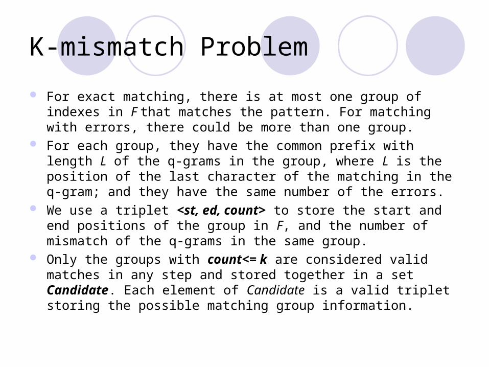
For exact matching, there is at most one group of indexes in F that matches the pattern. For matching with errors, there could be more than one group.
For each group, they have the common prefix with length L of the q-grams in the group, where L is the position of the last character of the matching in the q-gram; and they have the same number of the errors.
We use a triplet <st, ed, count> to store the start and end positions of the group in F, and the number of mismatch of the q-grams in the same group.
Only the groups with count<= k are considered valid matches in any step and stored together in a set Candidate. Each element of Candidate is a valid triplet storing the possible matching group information.

Extension of qgrep Algorithm
k-mismatch (P, C, Hr, Hrs, k)1. Initiate Candidate:
For each symbol , the c-th symbol in , do
create a triplet with
st = C[c];
ed = C[c+1]-1, if c < ,
= u, otherwise.
count = 0 if
=1 otherwise
if count <= k append the triplet to Candidate.
c
||
)1(Pc

Extension of qgrep Algorithm
2. for j = 2 to m do for each element in Candidate exists in (j-1)th iteration do
Remove the triplet (st, ed, count) from Candidate For each distinct symbol appears in F do
locate the start and end position st' and ed' in F between st and ed using binary search on the j-th column of the q-grams.
Note that we do not actually create the j-gram for each row in the q-gram matrix during binary search. Instead, given the row index pos of a q-gram in F, the j-th symbol s of the q-gram can be accessed in constant time as: s=F[Hr[Hrs[pos]+j]]
If = P(j), add triplet (st', ed', count) into Candidate. Since it is a match to P(j), there is no change with count.
Else, if count+1 <=k, add triplet (st', ed', count+1) into Candidate. Since an error occurred, count is incremented by one.
end end
3. Traverse Candate, report all the matches between st and ed in each element of Candidate. The position in F can be converted to the position in T, by Hrs.
c
c

Example
T=mississippi P=ssis k=2
P(1)=s P(2)=s P(3)=i P(4)=sF …. FS FST FSTT
1 I I X
2 I (1,4,1) ip (2,3,2) ipp X
3 I is (3,4,1) iss (3,4,2) issi X
4 I is iss issi
5 m (5,5,1) mi (5,5,2) mis X
6 P (6,7,1) pi (6,6,2) pi X
7 P pp (7,8,2) ppi (7,8,2) ppi X
8 S si (8,9,1) sip (8,8,2) sipp X
9 S (8,11,0) si sis (9,9,2) siss (9,9,2)
10 S ss (10,11,0) ssi (10,11,0) ssip(10,11,1)
11 S ss ssi ssis(10,11,0)

K-mismatch pattern matching results
K-mismatch (k=1)
0.0000
0.0005
0.0010
0.0015
0.0020
0.0025
0.0030
0.0035
0.0040
0.0045
0.0050
2 3 4 5 6 7 8 9 10 11
Word length
Tim
e (s
ec)
BWT
Suffix Tess
K-mismatch comparison for BWT qgrep and Suffix tree methods (k=1). The time is the average search time for a pattern over the corpus

K-mismatch pattern matching results
K-mismatch (k=2)
0.0000
0.0050
0.0100
0.0150
0.0200
0.0250
0.0300
0.0350
0.0400
0.0450
0.0500
3 4 5 6 7 8 9 10 11
Word length
Tim
e (s
ec)
BWT
Suffix Tree
K-mismatch comparison for BWT qgrep and Suffix tree methods (k=2). The time is the average search time for a pattern over the corpus

K-mismatch comparison for BWT qgrep and Suffix tree methods (k=3). The time is the average search time for a pattern over the corpus
K-mismatch pattern matching results
K-mismatch (k=3)
0.0000
0.0100
0.0200
0.0300
0.0400
0.0500
0.0600
0.0700
0.0800
0.0900
0.1000
4 5 6 7 8 9 10 11
Word length
Tim
e (s
ec)
BWT
Suffix Tree

K-mismatch pattern matching complexity Compressed Pattern Matching
Initial step: There are maximum m+2k-1 loops in stage 2
In j-th iteration there could be triplets generated. But will not be greater than u triplets.
Each triplet is found by a binary search on q-grams. The overall time complexity would be
The space complexity: We need O(u) space for auxiliary arrays and
to store the triplets.
)(O
j
/u
))/log(),min()2((2
uukmOkm
)),(min(2uO
km

Triplets Generated by qgrep
Triplet (#Peak)
1
10
100
1000
10000
2 3 4 5 6 7 8 9 10 11
Word length
k=1
k=2
k=3

Triplet(#Avg)
1
10
100
1000
10000
2 3 4 5 6 7 8 9 10 11
Word length
k=1
k=2
k=3
Triplets Generated by qgrep

Triplets generated by qgrep (example)
Peak (k=4)
48
477
1270
1994
546
158
220
500
1000
1500
2000
2500
1 2 3 4 5 6 7
Iteration
#tri
ple
ts
Peak

Clipped Suffix Tree for k-mismatch Problem Compressed Pattern Matching
The length of pattern is typically short maximum 50-100 characters.
Suffix tree can be built in O(u) time and O(m) search time, but O(21u) storage.
Build suffix tree with limited depth and perform searching.

K-approximate Problem
K-approximate match: given T and P, there exist at lease one r-length block of symbols in P that form an exact match to some r-length substring in T, where . (Baeza-Yates & Perleberg,1992)
1k
mr

K-approximate Problem
2 stages for k-approximate matching: Find r-grams using exact matching algorithms Verification

Ukkonen’s DFA construction time
m k=1 k=2 k=32 0.0005 0.0003 0.00033 0.0008 0.0008 0.00044 0.0013 0.0021 0.00195 0.0018 0.0045 0.00536 0.0023 0.0081 0.01337 0.003 0.0135 0.02938 0.0039 0.0188 0.05689 0.0049 0.0237 0.094210 0.0063 0.0296 0.140111 0.0079 0.035 0.184415 0.0118 0.056 0.28720 0.0167 0.08 0.5834 0.1 0.52 3.13

K-approximate Results
K-approximate matching (k=1)
0
1
2
3
4
5
6
7
8
9
2 3 4 5 6 7 8 9 10 11Word length
Tim
e (s
ec)
Agrep
Nrgrep
Bwt-Agrep
Bwt-Nrgrep
Bwt-DFA

K-approximate Results
k-approximat matching (k=2)
0
2
4
6
8
10
12
14
16
3 4 5 6 7 8 9 10 11
World length
Tim
e(se
c)
Agrep
Nrgrep
Bwt-Agrep
Bwt-Nrgrep
Bwt-DFA

K-approximate Results
k-approximate matching (k=3)
0
5
10
15
20
25
4 5 6 7 8 9 10 11Word length
Tim
e(se
c)
Agrep
Nrgrep
Bwt-Agrep
Bwt-Nrgrep
BWT-DFA

Outline
MotivationBackground and ReviewTransform Based Text CompressionCompressed Pattern MatchingSearch Aware Text Compression and
Retrieval Conclusion and Future Works
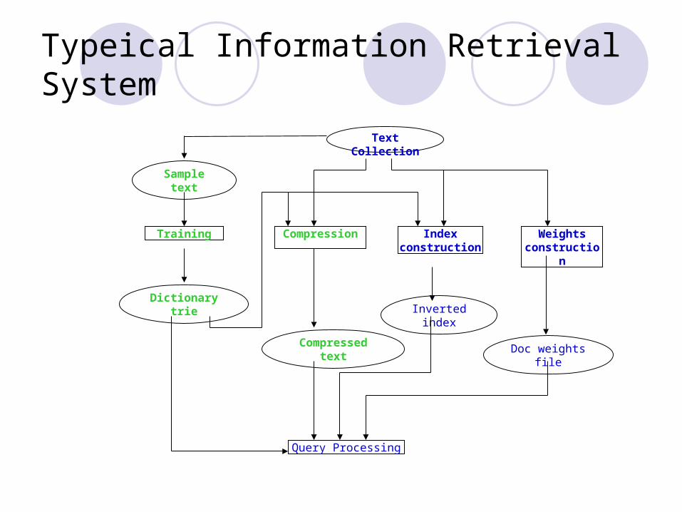
Typeical Information Retrieval System
Training
Sample text
Text Collection
Dictionary trie
Compression Index construction
Query Processing
Weights construction
Compressed text
Inverted index
Doc weights file
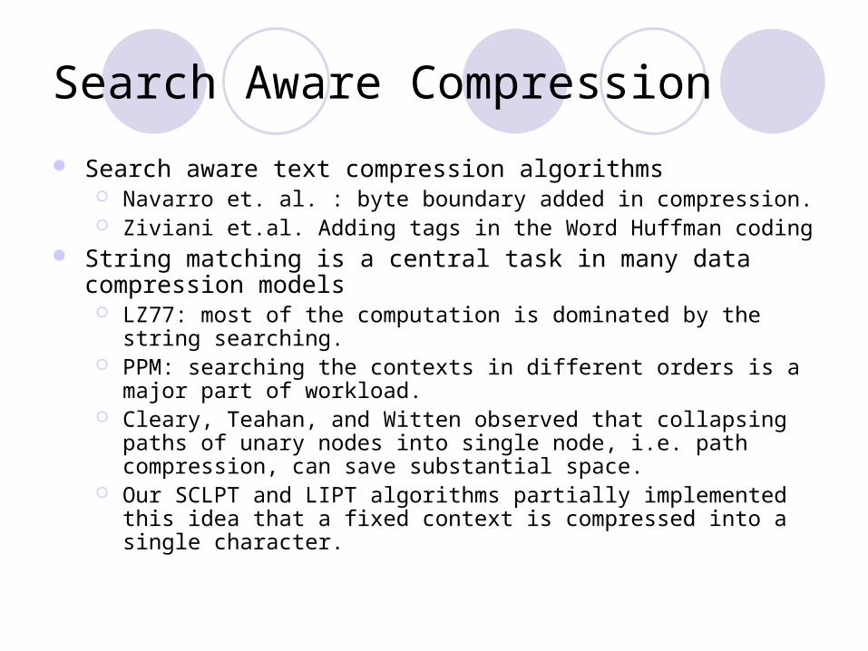
Search Aware Compression
Search aware text compression algorithms Navarro et. al. : byte boundary added in compression. Ziviani et.al. Adding tags in the Word Huffman coding
String matching is a central task in many data compression models LZ77: most of the computation is dominated by the string searching. PPM: searching the contexts in different orders is a major part of
workload. Cleary, Teahan, and Witten observed that collapsing paths of unary
nodes into single node, i.e. path compression, can save substantial space.
Our SCLPT and LIPT algorithms partially implemented this idea that a fixed context is compressed into a single character.

Search Aware Compression
Some observations (Larsson et.al): A context trie is equivalent to a suffix tree. The context trie of the PPM* model corresponds to a chain of nodes in
the suffix tree connected by suffix links. Using suffix links, a separate context list is not necessary to be maintained.
The characters that have non-zero counts in a context are exactly the ones for which the corresponding node in the trie has children. Hence there is no need for additional tables of counts for the contexts.

Search Aware Compression
Local suffix tree can be used in string matching in LZ and PPM algorithms.
On the other hand, suffix tree structure can be extracted from partially decompression of the file.
Fast search can be performed on suffix tree. Problem: select and combine local suffix tree for
the searching purpose

Random Access and Partial Decoding Using Modified LZW Algorithm
Efficient information retrieval in the compressed domain has become a major concern.
Being able to random access and partially decode the compressed data is highly desirable for efficient retrieval
Required in many applications. Example: in a library information retrieval system, only the records
that are relevant to the query are displayed. The efficiency of the random access and partial decoding depend
on the encoding/decoding scheme. Modified LZW algorithms:
Support fast random access and partial decoding to the compressed text.
The compression ratio is not degraded and may even be improved slightly using the modified LZW algorithm.

LZW Algorithm
An adaptive dictionary-based approach Build a dictionary based on the sequence that is being
compressed. The encoder begins with an initial dictionary consisting of
all the symbols in the alphabet. Dictionary built by adding new symbols to the dictionary
as it encounters new symbols in the text. The decoder can rebuild the dictionary as it decodes the
compressed text. The dictionary is actually represented by a trie. Each
edge in the trie is labeled by the symbols, and the path label from the root to any node in the trie gives the subsequence corresponding to the node.

Indexing for an LZW compressed file
The index of a pattern has a pointer containing the location of the occurrence of the keyword in the compressed stream.
Each keyword may have multiple pointers to the occurrences in the compressed text.
………. pattern 12, … ……………. ……………….. …………….. ………………
Keywords Indexes
3 8 9 4 6 2
1 2 3 ……. 10 11 12 13 14 ……
Inverted Index File
Data Stream

Modified LZW Algorithms
Original LZW: using beginning part of the text to build the trie and compress. Then continue compress using the fixed trained trie.
Offline LZW: using beginning part of the text to build the trie but not compress. Then continue compress using the fixed trained trie.
In above methods, each text has its own dictionary.
Public Trie: using a text collection to train the trie. Then all the text files will use the public trie to compress.

Compression Using Modified LZW

Index in Hierarchy
More details ->
current index level ->
Higher level ->Whole collection
documentsfile
documentsfile
paragraph
Higher level ->
paragraph paragraphparagraph
phrase phrasephrase phrase phrase phrase

Compression Performance
Avg. compression ratio
0.54
0.550.56
0.570.58
0.590.6
0.610.62
1 9 17 25 33 41 49 57 65 73 81 89 97 105 113
File ID
Co
mp
ress
ion
rati
o
The average compression ratio over the corpus using the trie from each file in the corpus
Compression Performance
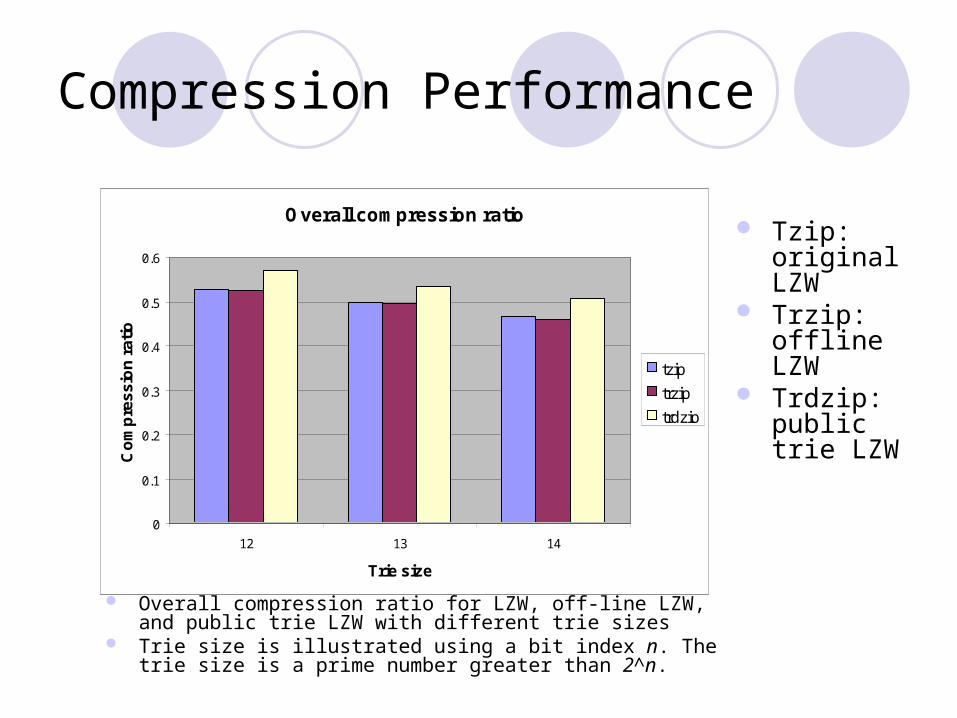
Overall compression ratio
0
0.1
0.2
0.3
0.4
0.5
0.6
12 13 14
Trie size
Co
mp
res
sio
n r
ati
o
tzip
trzip
trdzip
Tzip: original LZW
Trzip: offline LZW
Trdzip: public trie LZW
Overall compression ratio for LZW, off-line LZW, and public trie LZW with different trie sizes
Trie size is illustrated using a bit index n. The trie size is a prime number greater than 2^n.

Compression Performance
Compression ratio on a single file containing entire corpus
0.3
0.35
0.4
0.45
0.5
0.55
0.6
12 13 14
Trie size
Co
mp
ress
ion
rat
io
tzip
trzip
best trdzip(Avg. ratio)
best trdzip(overall)

Partial Decoding Performance
Compression Ratio Vs. File Size
0.4
0.42
0.44
0.46
0.48
0.5
0.52
0.54
0.56
0 1 2 3 4 5
File size (MB)
Co
mp
ress
ion
Rat
io
Trie size 12
Trie Size 13
Trie Size 14

Encoding time Vs File Size
Encoding time is linear to the file size.
Encoding Time Vs File Size (trzip)
0
1
2
3
4
5
6
0 0.5 1 1.5 2 2.5 3 3.5 4 4.5
File size (MB)
Tim
e(s)
Trie size 12
Trie Size 13
Trie Size 14

Decoding time Vs. Block Size
Decoding time is linear to the number of nodes.
Decoding time Vs. Block Size
0
0.2
0.4
0.6
0.8
1
1.2
1.4
1.6
1.8
0 512 1024 1536 2048
Block Size (number of encoded entries)
Dec
od
ing
tim
e(se
con
ds)
fo
r 10
0 ra
nd
om
blo
cks
200KB
500KB
1MB
2MB
4MB

Find an Optimal Public Trie
Train the initial trie with a size S. In experiment, we choose S to be 20 or 18.
For each node, recode the count for the number of access.
Remove the leaf node with the lowest count (if there are multiple leaves with the lowest count, pick one arbitrarily) until the target trie size is reached.

Compression Ratio vs. Trie size (code length)
0
0. 1
0. 2
0. 3
0. 4
0. 5
0. 6
12 13 14 16 18 20
Tri e Si ze
Comp
ress
ion
Rati
o

Possible Parallel Processing
The code is fixed length 16bit (2 bytes). Text can be segmented to different blocks. Encoding:
Each block is compressed by a single Processor. Then concatenate the results.
Decoding: Random access Can decoding from any point with an even number of
bytes after header.

Compression Ration vs. Random Access
Raw Text*
Com
pression
ratio
Levels of details
better PPM*
WordHuff*MLZW
*
BWT*XRAY
*
Symbol | | FileBlock |Phrase |
gzip*

Outline
MotivationBackground and ReviewTransform Based Text CompressionCompressed Pattern MatchingSearch Aware Text Compression and
Retrieval Conclusion and Future Works
Conclusion and Future Works
We have presented the novel algorithms for lossless text compression using transformation with static dictionary.
The limitation: only English dictionary is used and tested on the limited amount of the text data. Text in different language or domain specific. A universal Solution.
Conclusion and Future Works
Compressed Pattern Matching on BWT based compression up to MTF stage Search with regular expression, wildcard
symbols. Search to further stage. Deal with long sequences.

Conclusion and Future Works
Our novel approach to incorporate the current compression algorithm and the index based text retrieval provide a solution to handle the compression and partial decompression in the low level without touching the high level query evaluation. Better Public Trie Training algorithm. Other search aware compression scheme. Implementation in a parallel/distributed environment.