This is a manuscript version. The article has been accepted for publication in the Journal of Urban Economics.

Transfer Taxes and Household Mobility:

Distortion on the Housing or Labor Market?*

Christian A. L. Hilber

London School of Economics, Centre for Economic Performance (CEP) & Spatial Economics Research Centre (SERC)

and

Teemu Lyytikäinen

VATT Institute for Economic Research & Spatial Economics Research Centre (SERC)

Original submission: September 10, 2015 First revised version: July 21, 2016

Second revised version: June 10, 2017 Accepted: June 15, 2017

* This paper replaces an earlier version entitled “The Effect of the UK Stamp Duty Land Tax on Household Mobility” (SERC Discussion Paper No. 115, July 2012). We thank David Albouy, James Banks, Florian Mayneris, Henry Overman, Jos Van Ommeren, Yasusada Murata, and participants at the Barcelona Economics Institute IEB, the cemmap/IFS workshop on ‘Housing: Micro Data, macro Problems’, the Finnish Economic Association Meeting in Vaasa, the London School of Economics, the Tinbergen Institute, the Helsinki Center for Economic Research, the Meetings of the Urban Economics Association in Miami (2011) and in Lisbon (2015), the II Workshop on Urban Economics in Barcelona, two anonymous referees and the Editor, Matt Turner, for helpful comments and suggestions. Lyytikäinen acknowledges financial support from the Academy of Finland through the Economics of Housing II project. All errors are the sole responsibility of the authors. Address correspondence to: Christian Hilber, London School of Economics, Department of Geography and Environment, Houghton Street, London WC2A 2AE, United Kingdom. Phone: +44-20-7107-5016. Fax: +44-20-7955-7412. E-mail: c.hilber@lse.ac.uk. © 2017. This manuscript version is made available under the CC-BY-NC-ND 4.0 license http://creativecommons.org/licenses/by-nc-nd/4.0

 

Transfer Taxes and Household Mobility:

Distortion on the Housing or Labor Market?

Abstract

We estimate the effect of the UK Stamp Duty Land Tax (SDLT) – a transfer tax on the

purchase price of property or land – on different types of household mobility using micro

data. Exploiting a discontinuity in the tax schedule, we isolate the impact of the tax from

other determinants of mobility. We compare homeowners with self-assessed house values on

either sides of a cut-off value where the tax rate jumps from 1 to 3 percent. We find that a

higher SDLT has a strong negative impact on housing-related and short distance moves but

does not adversely affect job-induced or long distance mobility. Overall, our results suggest

that transfer taxes may mainly distort housing rather than labor markets.

JEL classification: D23, H21, H27, J61, R21, R31, R38.

Key words: Transfer taxes, stamp duty, transaction costs,

homeownership, household mobility.

1  

1. Introduction

Most developed countries impose a tax on transactions of property and land. This tax – in North America often labelled ‘land transfer tax’ and in Britain ‘stamp duty’ – increases the transaction costs associated with the sale of a property and therefore increases the costs of moving for homeowners. This cost increase can be expected to negatively affect the propensity to move. Thus, the tax is prone to have adverse effects on housing and labor markets. Households may not live in the type of dwelling and the location that most closely match their preferences. Similarly, individuals may be less willing to accept new jobs that are not within commuting distance or they may decide to hold on to a current job that is a less good match than another available job further away. Given these potential adverse effects caused by mismatch in housing and labor markets, the question of whether, and to what extent, the tax reduces household mobility is highly policy relevant.

Transfer taxes and in particular the UK Stamp Duty Land Tax (SDLT) – commonly referred to as ‘stamp duty’ – have long been criticized by economists as being inefficient. The Mirrlees Review (2011) highlights the fact that the SDLT “creates a disincentive for people to move house” (p. 403) and the adverse consequences of this on the functioning of housing and labor markets. To date, however, little is known about the nature of the moves (short vs. long distance or housing- vs. job-related) that are most strongly adversely affected. This is the key focus of our study.

The UK stamp duty scheme in place until December 3, 2014 provides an ideal setting to explore the impact of transfer taxes on mobility decisions. This is partly because the tax liability was quite substantial, at least for more expensive housing (the top rate until December 3, 2014 was 7 percent, levied on the entire purchase price), and partly because the stamp duty liability jumped sharply at various cut-off values, providing various ‘discontinuities’ that can be exploited empirically.1 Our analysis focuses on a discontinuity – or ‘notch’ – where the stamp duty jumps particularly strongly. This notch – at £250k – allows us to isolate the impact of the stamp duty from other determinants of mobility.

Basic economic intuition and simple theoretical considerations suggest that different types of moves may be differentially affected by the stamp duty. This is because benefits from moving are likely larger for more momentous – employment- or life event-related – mobility shocks than for more gradual changes in life-cycle circumstances – which typically move homeowners away incrementally from their optimal location and housing consumptions. Our theoretical considerations yield three empirically testable predictions: (i) At the house value cut-off of £250k, as a consequence of the tax notch, household mobility should decrease; (ii) The adverse impact of the notch should be greater for (more incremental) short distance moves than for (more momentous) long distance ones; and (iii) The adverse effect should be greater for (more gradual) housing-related than for (more momentous) job-related moves.

To test these predictions, we use data from the British Household Panel Survey (BHPS) and compare homeowners with self-assessed house values on either side of the cut-off, while

                                                            1 The reform from December 3, 2014 removed these discontinuities.

2  

controlling for flexible but smooth functions of house values. Consistent with our theoretical priors, we find that the SDLT has a significant negative effect on household mobility. Moreover, this adverse effect is confined to short distance moves and to moves that are housing-related. We find no significant effect on job-related moves and we find little evidence that the stamp duty adversely affects moves that are triggered by major ‘life events’ such as divorce or retirement. We document these key results both visually and using rigorous regression analysis.

Our core estimate indicates that the 2 percentage-point increase in the SDLT reduces the annual rate of mobility by 2.6 percentage points. This is a substantive effect given that the estimated counterfactual mobility rate in the group affected by the tax rate increase is only 7 percent. It equates to a 37 percent decrease in mobility. The corresponding welfare loss in the form of distortions in the housing market is very substantial. Based on our central point estimate, simple calculations imply that the welfare loss associated with the rate increase from 1 to 3 percent could be in the range of about 40 to 80 percent of the additional revenue generated by the tax increase.

In conducting our analysis we faced a number of empirical challenges. Some of these are specific to our underlying data and research design. A key concern is that homeowners with higher underlying propensity to move may be better informed about the stamp duty and may therefore be more likely to report the cut-off value rather than a value slightly above (i.e., sorting of homeowners close to the cut-off could partially drive our findings). Another potential sorting mechanism is that households that are interested in moving may attempt to keep the value of their house below the cut-off by neglecting renovation. To address these potential sorting issues, we drop households that self-report the cut-off value (or values very close to it) in a robustness check. Our results become less precise but the key findings regarding differential impacts of the stamp duty on different types of mobility remain clear. We also carried out a battery of ‘balancing tests’ to check for sorting of households with different characteristics around the cut-off. In addition, we perform a robustness check where we limit the sample to households who responded in the survey that they would like to move. For this sub-sample, sorting based on unobserved willingness to move should be a lesser concern. Our key findings are robust to all these checks.

Overall, our results confirm the findings of the previous literature that transfer taxes are highly distortive in that they substantially reduce mobility. The main novel contribution of our study is that we demonstrate that these distortions are largely confined to short distance and housing-related moves.

Two strands of the economics literature motivate our analysis. The first strand is the existing literature on the impact of transfer taxes on household mobility. Transfer taxes are an important part of housing transaction/moving costs and they are the most important component directly determined by policy makers. Despite this, little is known about their effect on mobility. On the theoretical side, Lundborg and Skedinger (1999) modify Wheaton’s (1990) seminal search model of the housing market by adding transfer taxes into

3  

the framework. They derive that the lock-in effects of the tax reduce welfare, with the adverse effect being larger at low vacancy rates and smaller with a buyer tax. The latter is because the buyer tax-induced price reduction dampens the negative effect on search effort caused by the tax. Nordvik (2001) analyzes the mobility effects of transfer taxes in a theoretical dynamic life-cycle model of housing demand. He finds that a transfer tax rate of 2.5 percent decreases the number of moves by the model household over the life cycle from three to one, implying substantial dead-weight losses.

On the empirical side, Van Ommeren and Van Leuvensteijn (2005) provide indirect evidence on the mobility effects of transfer taxes using individual panel data for the Netherlands. They estimate a competing risks hazard model of moving to renting or owning with house values as an explanatory variable and use a theoretical model to infer the effect of transaction costs. Their results suggest that a 1 percentage-point increase in the value of transaction costs—as a percentage of the value of the residence—decreases residential mobility rates by at least 8 percent.

Dachis et al. (2012) utilize the introduction of land transfer taxes in Toronto to estimate their effect on the housing transaction volume and prices with a Differences–in-Differences approach, comparing market outcomes across the boundary of the affected area.2 According to their estimates, a 1.1 percent land transfer tax led to a 15 percent decrease in transactions in the first eight months after the introduction. The implied welfare loss relative to an equivalent property tax is about $1 for every $8 in tax revenue.

Discontinuities in transfer tax schedules have recently attracted increasing attention as a source of insight into how the tax affects market outcomes. Most closely related to the present paper, Best and Kleven (2015) utilize (i) administrative data on all property transactions in the UK, (ii) the discontinuities in the UK schedule to study price responses and (iii) changes in the tax schedule over time to study the effect on the transaction volume. Best and Kleven (2015) provide evidence of a strong negative price effect. In addition, they document that a temporary 1 percentage-point cut in the tax rate – due to the 2008-9 stamp duty holiday on houses worth between £125,001 and £175,000 – led to a 20 percent increase in transactions. The bulk of this impact is explained by a long term reduction in sales rather than the timing of purchases.

Besley et al. (2014) exploit the same 2008-9 stamp duty holiday to estimate the incidence of a transaction tax on housing. Their key findings are twofold. First, around 60 percent of the “surplus” due to the tax holiday accrued to buyers. Second, the tax holiday increased transactions of properties by about 8 percent but this effect was only short-lived. The effect reversed rapidly after the policy was withdrawn.

In a similar vein – exploiting a tax notch imposed by New York’s so called ‘mansion tax’ – Kopczuk and Munroe (2015) find robust evidence of substantial bunching (both buyers and sellers have strong incentives not to transact near the threshold). Moreover, they document

                                                            2 See also Dachis (2012) for follow-up work using a longer data period.

4  

that the incidence of the mansion tax falls on the seller, may exceed the value of the tax, and cannot be explained by tax evasion.

Davidoff and Leigh (2013), finally, explore the incidence of transfer taxes using data from Australia where the marginal tax rate rather than the average tax rate jumps at various cut-off prices. They use past local house prices and national house price inflation to construct an instrumental variable for the transfer tax rate. Their results indicate that a higher tax rate reduces turnover and – in line with Kopczuk and Munroe’s findings (2015) – the incidence of the tax is on the seller.

The second strand of the literature that motivates our analysis explores the link between homeownership and labor market outcomes. It is a well-established fact that homeownership induces significant barriers to mobility – transfer taxes are one important component of such barriers. In a seminal paper Oswald (1996) argues that homeownership, by reducing mobility, increases unemployment. Moreover, he provides cross-country evidence consistent with this conjecture. Subsequent studies (e.g., Van Leuvensteijn and Koning, 2004; Munch et al., 2006 and 2008; Battu et al., 2008) that use individual-level panel data and more rigorous estimating techniques, by and large, confirm Oswald’s conjecture that homeowners are less mobile. They rebut, however, the hypotheses that homeowners are more likely to become unemployed or have longer unemployment spells.3

Coulson and Fisher (2009) explore a number of theoretical mechanisms that may affect the link between homeownership on the one hand and mobility and labor market outcomes on the other hand. They point out that different theoretical models can have very different predictions about the labor market at both micro and aggregate level. Their findings suggest that homeowners are less likely to be unemployed but they also have lower wages than renters. At the aggregate level, higher regional homeownership rates are associated with a greater probability of individual worker unemployment and higher wages.

Finally, Ferreira et al. (2010 and 2011) point out that there may be an asymmetry in the mobility response of homeowners depending on whether or not they are in negative equity. Whereas their findings indicate that homeowners in negative equity are indeed less likely to move, other empirical studies (Schulhofer-Wohl, 2011; Coulson and Grieco, 2012) reach the conclusion that homeowners who are under water are slightly more likely to move than homeowners with positive equity.

                                                            3 Van Leuvensteijn and Koning (2004) find no evidence that homeowners change jobs less than tenants. They conclude that the housing decision is driven by job commitment (and not the reverse) and that homeowners are less vulnerable to unemployment. Munch et al. (2006) point out that homeowners may set lower reservation wages for accepting jobs in the local labor market. Hence, they are more likely than renters to find jobs locally. Munch et al. (2008) have argued, from a search theoretic perspective, that homeowners should have a lower transition rate into new non-local jobs and therefore should stay longer in their jobs. Battu et al. (2008) suggest that there are differential effects across tenure types and that it matters whether the starting point is employment or unemployment. Their findings imply that homeownership is a constraint for the employed and public renting is more of a constraint for the unemployed.

5  

The general lesson learned from this literature is that policies that make households less mobile may harmfully affect the performance of housing and labor markets. Our study contributes to this literature by demonstrating that transfer taxes prevent moves driven by more incremental life cycle changes (such as short distance and housing-related mobility) but they do not preclude moves driven by more momentous shocks (long distance and job-related mobility).

2. The UK stamp duty system and theoretical considerations

The stamp duty on transactions on property and land was introduced in the UK during the 1950s. We focus on the system of stamp duty on residential transactions that had been in place until December 3, 2014.

The stamp duty is paid by the buyer and is a percentage share of the purchase price of the house. The economic incidence, however – in line with the literature discussed in Section 1 – can be expected to mainly fall on the seller.

The defining feature of the UK stamp duty system (i.e., the one in place until December 3, 2014) is a progressive schedule where the tax rate for the whole purchase price goes up at certain thresholds. Table 1 reports the tax schedule that applies during our sample period: Houses sold for up to 125,000 are exempt from stamp duty, but from £125,000 upwards the tax rate rises in a stepwise manner from 1 to 5 percent.4

Our empirical analysis focuses on the second cut-off at £250,000 where the tax rate increases from 1 to 3 percent. We do so because stamp duty payable increases significantly at the cut-off (from £2,500 to £7,500)5, and because our data is reasonably dense around the £250k cut-off.6 Significant variation in stamp duty liabilities and large sample size together make it possible to detect the effects of the stamp duty on mobility.

When households make their relocation decisions they take into account expected benefits as well as expected costs of moving. Basic economic intuition suggests that the stamp duty increases these costs.7 When buyer and seller bargain over the agreed transaction price, a

                                                            4 A new higher “mansion” tax rate of 7 percent (or 15 percent for corporate bodies) was introduced for properties over £2 million on 22 March 2012. A tax ‘holiday’ was in place on properties worth between £125 and £175 during 2008-9. None of these changes affected the notch we investigate. 5 At the £125k cut-off the treatment is much weaker as the tax liability rises only by £1,250. Moreover, this cut-off is subject to various regional exemptions and we do not know whether the survey respondents in our BHPS sample are subject to such an exemption. 6 Lack of density around the cut-offs rules out using the thresholds of £500k and £1m. We also note that while the jumps in tax liability are £5k and £10k, respectively, for these two cut-offs, these jumps are smaller in ‘relative terms’ as only fairly high income and wealthy households will be able to afford to buy houses worth over £500k and especially over £1m. 7 A household move does not necessarily induce a housing transaction. Households may hold on to their old homes and rent them out, while at the same time buying new ones. This is not very common, however, in part because (i) many households need the sales proceeds for their next down-payments, (ii) most homeowners do not want to be landlords, and (iii) certain housing stock (single-family housing) may be more suitable for owner-occupation (Linneman, 1985). Hence, the effect of transaction taxes on mobility and on transactions is in practice closely correlated. Transfer taxes may also affect the propensity that households choose to become

6  

transaction can only occur if the buyer’s valuation of the seller’s house exceeds the seller’s valuation by a sufficiently large margin to overcome the transfer tax. If the transfer tax increases, the propensity of a transaction decreases implying a lower likelihood that the seller

moves.8 These considerations yield our first empirically testable prediction: At the house value cut-off of £250k, as a consequence of the stamp duty tax notch, household mobility should decrease (Prediction 1).

We would expect that the magnitude of the adverse effect of the stamp duty on mobility depends on household specific circumstances. Homeowners who face gradual changes in their life-cycle circumstances – which move them away incrementally from their optimal locations and housing consumptions – may be strongly discouraged from moving as a consequence of a jump in the stamp duty. This is because the benefits of moving often only exceed the costs by a narrow margin; a leap in the stamp duty renders these moves nonviable. In contrast, the relocation decisions of homeowners who face rarer but more momentous – typically employment-related – mobility shocks may be less affected by an increase in the stamp duty: Employment-related large mobility shocks, especially if there are no suitable jobs available locally, tend to trigger substantial benefits arising from relocation and these often exceed the stamp duty-induced costs of moving by a wide margin.9 The corresponding empirical predictions are that the adverse effect of the stamp duty increase on household mobility should be greater for shorter distance moves than for longer distance ones (Prediction 2) and for housing-related as opposed to job-related moves (Prediction 3).10

3. Empirical analysis

3.1. British Household Panel Survey (BHPS) data

The data used in this study is derived from the BHPS. The BHPS follows roughly 10,000 households over time. We use data from 1996 to 2008, which is the last year available.11 The surveys for each wave are conducted between September and March. We define our ‘year’ variable as the year when data collection started.

                                                                                                                                                                                         homeowners (and, possibly, the aggregate housing consumption over their life cycle). Households – especially those with a short expected duration – can be expected to become renters because the moving costs are high. The effect of the transfer tax on tenure choice is a question that should be explored in future work. 8 This simple economic intuition could be formalized in a Nash bargaining framework that models utility as a function of amenities and income opportunities. Such formalization is beyond the scope of this paper. 9 We note however that localized amenity shocks are not necessarily smaller than income shocks. For example, Linden and Rockoff (2008) show that prices of homes near sex offenders decline considerably following an offender’s arrival in the neighbourhood. 10 Prediction 2 is reinforced by the fact that costs related to different types of moves likely differ: Long distance moves, such as moving to another labour market area, may entail higher psychic costs due to a loss of existing social networks, than moves related to adjustments of housing consumption in the same area (see Kennan and Walker, 2011). If the underlying relocation costs are higher, the stamp duty represents a relatively smaller addition to the cost and therefore it is likely that the stamp duty affects long distance moves to a lesser extent than short distance ones. 11 The BHPS was subsequently replaced by the Understanding Society survey and there was a break in the panel.

7  

In addition to a rich set of household characteristics, the dataset includes the owner-occupiers’ assessments of the value of their homes and information on whether the household moved in the subsequent year, making it an ideal dataset to study the impact of transfer taxes on household mobility. The exact question on which the self-assessed house value is based is: “About how much would you expect to get for your home if you sold it today?” If the household gives a range, the interviewer will report the lowest figure in that range.

The self-assessed house value variable is effectively discrete in nature. In theory survey respondents could state any value. In practice however there are observations only at 147 values within the broadest band we use (£150k to £350k). 97.7 percent of the observations are concentrated at values divisible by £5k. We round house values up to the closest value divisible by £5k and use this variable in our econometric analysis to avert issues related to statistical inference discussed in Section 3.2.

In our empirical analysis we essentially compare households reporting house values above the 250k cut-off, where the stamp duty tax rate jumps from 1 to 3 percent, with households with self-reported values below the cut-off. We limit the sample to owner-occupiers with self-assessed house values within 20, 30 or 40 percent of the £250k cut-off value (+/- £50k, +/- £75k and +/- £100k, excluding endpoints).

One limitation of our analysis is that the mobility status of the last wave (2008) is not known. Thus, the estimation sample consists of data from 1996 to 2007. Finally, we exclude households that moved into their current dwelling between year t-2 and t. We do this because recent movers can be expected to be overrepresented below the £250k cut-off which could bias our estimates (see the discussion in Section 3.2).

Figure 1 Panel A shows the distribution of self-assessed house values in 2006. Overall, people tend to report round values divisible by £50k. There is a clear spike at £250k, but this spike does not stand out from the other round values. Panel B of Figure 1 illustrates the distribution of actual transaction prices in the UK in 2006 from a data set obtained from the Land Registry. We expect to observe a pile-up in the transaction price distribution at £250k because houses that would sell for up to £255k absent of the tax rate notch will sell for £250k. This is indeed what the figure reveals. The bunching at the threshold is clearly much more pronounced in the transaction price distribution depicted in Panel B of Figure 1 than in self assessed house values. The fact that there is no abnormal pile-up at the cut-off in Panel A of Figure 1 supports the validity of our empirical strategy.

Treatment variable

Our treatment variable is a dummy that equals one if the self-assessed house value of household i in year t exceeds £250k, Treatit = D(House valueit > 250k). We argue that the likelihood that the household’s moving decision is affected by the 3 percent tax rate rather than the 1 percent rate increases drastically at, or in the vicinity, of this point. The self-assessed value may not be an accurate measure of the actual value when a house is sold. However, the self-assessed value is arguably more relevant for our purposes as households’

8  

expectations regarding stamp duty payable upon sale are likely based on the self-assessed house value.

Outcome variables

Our outcome variable measures actual moves between the interview date and the subsequent interview. The variable Moveit gets the value one if the BHPS records classify the household as a mover household in t+1. We lose some observations due to attrition from the panel between t and t+1 but we were able to recover the value of the moving indicator for some non-respondent households by utilizing information in the sample record files of the BHPS. In addition to the overall mobility, we study different types of mobility separately by using information on the distance of move and main reasons of moving.

We argue that a direct measure of household mobility is preferable to measures of housing transactions, used in most previous studies, when the interest is on the potential adverse impact of the transfer tax on the functioning of housing and labor markets. The crucial advantage of the BHPS with respect to our core research question is that it allows us to gain insight into the effects of transfer taxes by analyzing different types of moves.

Round values

Exploring the data suggests that households that report round house values divisible by £50k (£150k, £200k etc.) have a lower propensity to move. One might be concerned that households intending to stay do not follow the market as closely and give rough rounded estimates of the value of their house. The round value effect might bias our estimates if disproportionately many round values are in the treatment or the control group. To address this issue, we include a dummy variable for round house values divisible by £50k in the model as a control variable.

Summary statistics

Table 2 presents summary statistics for the variables used in our empirical analysis for the largest regression sample (40 percent band around the cut-off). The average house value in the sample is £220,000 and 4.4 percent of households moved within a year. To analyze whether different types of moves are differentially affected, we divide moves into two categories based on the distance of move: less than 10km, and 10km or more. In addition, we use information about the main reason for the move to construct three categories: ‘housing- and area-related’, ‘employment-related’ and ‘life event-related’. The categories are described in detail in Appendix Table A1. Housing- and area-related reasons are most common. Moves motivated mainly by job-related reasons seem to be rare. This may partly reflect how the survey question is formulated. Employment motives may still be important even if they are not the main reason for the move. Moving distance and main reason for move being employment related are strongly positively correlated and we think that by analyzing the distance of move we can gain additional insight into whether transfer taxes hinder relocation of the workforce. Less than one percent of short distance moves (defined as less than 10km)

9  

but about 11 percent of moves beyond 10km are mainly job-related. Similarly, 56 percent of short distance moves but only 27 percent of long distance moves are mainly housing-related. Life event-related mobility is not strongly correlated with the distance of move.

3.2. Empirical approach

Obstacles to causal inference

Our empirical approach exploits the fact that the stamp duty jumps substantially at the threshold of £250k. This discontinuity creates variation that can be used to isolate the impact of the stamp duty from confounding factors. Theory predicts that owners who possess homes that are worth less than £250k should be more likely to move than otherwise similar ‘treated’ owners with homes worth above £250k. In an ideal world, from an econometric point of view, house values would be exogenously determined and precisely measured. In such a setting, the treatment status is as good as random very close to the threshold. This is a regression discontinuity design (RDD) discussed in Lee and Lemieux (2010).

Our empirical approach has the features of an RDD but differs from the ideal setting in important ways, creating obstacles to causal inference. First, our assignment variable is essentially discrete, which means that it is impossible to compare outcomes for households just above and just below the cut-off where the stamp duty increases (Lee and Card, 2008). We have to choose a functional form for the relationship between house values and mobility, and use observations both close and relatively far from the cut-off to estimate this relationship. We use data within 20, 30 or 40 percent of the cut-off value and approximate the relationship between mobility and house values through flexible but smooth functions (polynomials) of the self-assessed house value, which we include in the set of control variables. We do the latter to address the potential issue that other determinants of mobility correlated with house values might bias our results.

A second obstacle to causal inference is that we cannot be sure whether all households that report house values above the limit are affected by the 3 percent tax rate (or whether households below the limit are affected by the 1 percent tax rate). Households that report house values close to the cut-off might attach some probability to being on the other side of the cut-off. People near the 250k cut-off are likely to have the same expectations about the sales price, so we might not expect to see a jump in behavior across this cut-off when focusing on observations very close to it. This implies that the treatment group indicator likely measures actual treatment status with error which would lead to attenuation bias towards zero.12 This attenuation bias should decrease and eventually disappear however when we compare house values further from the cut-off.

                                                            12 Our empirical model resembles a reduced form of a fuzzy RD design. Standard fuzzy RD analysis uses a discontinuity in the likelihood of obtaining the treatment as an instrument for the actual treatment status in a Two-Stage-Least-Squares regression. This approach is not feasible with the BHPS data because there is no way to identify the treated households with certainty.

10  

The third and arguably the most important obstacle to causal inference is the fact that in our setting the assignment variable – the self-assessed house value – is in principle a choice variable.13 Although survey respondents in the BHPS have no incentive to misreport the value of their home, both the actual value (quality) of the house and the reporting of the value can be influenced by the owner.

This is an obvious concern for recent movers. These movers are disproportionately represented just below the cut-off because many houses sell at and just below £250k. To the extent that the recent mover status affects mobility, this may bias our estimates. Moreover, recent movers may be problematic for our research design in the sense that they can precisely choose the value of their house. Their ability to “precisely manipulate” the assignment variable can invalidate our research design. Due to these issues, we exclude households that moved into their current dwelling between year t-2 and t.14 We analyze the robustness of our findings to this sample restriction in a Web Appendix (Tables W1-W4).

There are two further potential sorting mechanisms that could threaten causal inference. First, households that are interested in moving could try to keep the value of their house below the cut-off by neglecting renovation. Such behavior is unlikely to lead to drastic bunching below the cut-off because local demand and supply conditions are the main drivers of house prices and therefore precise manipulation through maintenance seems infeasible. To the extent such behavior nevertheless occurs, unobserved willingness to move may bias our estimates as households may sort based on this unobservable characteristic. Second, manipulation of the running variable can occur if people anticipate that it is difficult to sell the house just above the cut-off and therefore report self-assessed house values just to the left of the cut-off. This should show up as bunching at the cut-off value. If households that consider moving are better informed about the stamp duty cut-off, this may lead to sorting around the cut-off based on the underlying propensity to move. To the extent such sorting does indeed occur, this could create an upward bias in the estimated impact of the tax.

To address these two sorting related concerns, we carry out extensive validity and robustness checks. First, we demonstrate that there is no abnormal mass in self-assessed house values below the cut-off (see Figure 1, Panel A), indicating that manipulation may not be a significant concern.15 Second, because potential manipulation would be likely to occur very

                                                            13 The use of self-assessed house values instead of actual transaction prices (that actually determine the treatment) is partly a necessity in the context of our analysis. This is because we are interested in how transfer taxes affect the propensity of different types of moves occurring. The BHPS provides detailed information on the nature of the moves and on the intention of households whether to move, but it does not provide actual transaction price data. Moreover, self-assessed house values are available regardless of whether houses are sold, implying that we can determine the treatment status of all owner-occupier households. 14 We conducted balancing tests to determine the appropriate time window and find indication of sorting of households that moved between year t-2 and t. Hence, we dropped these households from our sample. We do not detect any discontinuity for less recent movers. The balancing tests are reported in Web Appendix Table W5. 15 McCrary (2008) type formal tests of discontinuity in the distribution of house values are not suitable with our data. This is because the strong concentration of the data in round values could be erroneously interpreted as manipulation.

11  

close to the threshold, we test whether dropping observations near the threshold (“donut approach”) changes our conclusions. However, this is not the case. Third, we run balancing tests where we test for discontinuities in observable household characteristics at the threshold. Detecting such discontinuities would be indicative of sorting that could bias our results. However, we find little evidence for such discontinuities. Fourth, we test whether our results are robust to the inclusion of household characteristics as additional controls. This is indeed the case. Finally, we redo our analysis, focusing exclusively on a sub-sample of households that are willing to move. (We derive this information from a survey question.) For this subsample, sorting based on interest in moving should not be a concern. Our results are qualitatively very similar.

Given the three obstacles to causal inference, one option could be to ignore values close to the cut-off entirely and focus solely on values further away as our main specification. For such a sample sorting and attenuation bias are not a concern. Including values close to the cut-off however has the advantage that treatment and control group are more similar in their characteristics and that we can estimate the treatment effect more precisely. Moreover, and importantly, all our validity and robustness checks are suggestive that sorting and attenuation bias are not driving our findings, advocating not dropping observations very close to the cut-off.

Empirical specification

We estimate a regression model of a mobility dummy on a dummy for the self-assessed house value being above the £250k cut-off. We include a flexible but smooth function of house values in the set of control variables. We do this because other determinants of mobility could be correlated with the self-assessed house value, on which the treatment indicator is based. The house value variables are intended to pick up the impact of all determinants of mobility correlated with house values, apart from the stamp duty. Specifically, we estimate:

Moveit = βt+ β1Treatit+ f(House Valueit)+ uit , (1)

where the dependent variable Moveit is the mobility indicator that gets the value one if household i moved between year t and t+1. The treatment variable takes the value one if the household’s self-assessed house value exceeds £250k. The function f(House Valueit) is a 1st – 4th order polynomial of the self-assessed house value. In addition, we test the robustness of the results to allowing for different polynomials on either side of the cut-off. A dummy for round values divisible by £50k is included as an additional control.

The identifying assumption of the model is that variable Treatit is uncorrelated with the error term conditional on f(House Valueit). This assumption is satisfied if other determinants of mobility develop smoothly with respect to house values and are therefore captured by the f function. The ability of households to precisely manipulate whether they are to the right or to the left of the cut-off could lead to discontinuities in other determinants of mobility and

12  

invalidate the identifying assumption. The numerous validity and robustness checks reported in the results section are designed to dispel this concern.

The main focus of our analysis is the differential impact of the stamp duty on different types of mobility. The assumption required for identifying the differential impacts is less stringent than for unbiased estimation of the impact on the overall mobility rate. This is because any endogeneity issues likely affect the estimates for different types of mobility similarly. Thus, even if the estimates for the magnitude of the effect were biased, qualitative conclusions regarding differences in the impact of the stamp duty on different types of moves likely remain valid.

External validity

If all households respond similarly to the stamp duty, our results for the £250k cut-off can be generalized to apply for the whole population in the UK and possibly tell us something about the effects of similar taxes in other countries as well. With heterogeneous responses, the results may apply to a smaller sub-population. Drawing on Lee and Lemieux (2010), our estimates can be interpreted as a weighted average of treatment effects of the British owner-occupier households in the BHPS data. The weight of each household is the probability that their self-assessed house value falls within the band around the cut-off used in each specification we estimate. A further limitation to the external validity of our results is that we constrain the sample to households that have not moved during the two previous years. Thus, the sample is not representative of all homeowners.

Statistical inference

The panel property of the data and the lumpiness of the distribution of self-assessed house values have potential implications for statistical inference. Firstly, since the households in our sample are observed in multiple years, we have to account for within household correlation of the error terms through clustering by household. Another potential issue regarding statistical inference was pointed out by Lee and Card (2008), who discuss RD analysis with a discrete assignment variable. They argue that specification errors in the fitted regression line imply that at each discrete value there is an error component positively correlated within observations at that particular point, which means that standard errors are downward biased. They show that clustering standard errors by the values of the discrete assignment variable solves the problem. As explained above, we round house values up to the closest £5k multiple. We cluster the error terms at the household level and £5k house value group level in our analysis. In some cases, especially with the 20 percent band, two-way clustering produces lower standard errors than clustering at household level only. This is likely due to an insufficient number of house value clusters. In these cases, we report the higher of the two standard errors. In order to test whether our statistical inference might be biased, we run placebo tests where we apply our method to artificial cut-offs set at £5k intervals (between £150k and £350k), and show that we do not find overly many false significant coefficients.

13  

3.3. Results

We start with results on the impact of the stamp duty increase on observed household mobility. Figure 2 provides a descriptive analysis of mobility and illustrates our econometric results, with the circles depicting the mobility rate for £10k wide house value groups. The size of the circle is proportionate to the number of observations in the group. The line in Panel A of Figure 2 shows predicted mobility rates from model (1) with a 4th order polynomial of house values, and the band around it represents the 95% confidence interval. Consistent with Prediction 1, the figure reveals that there is a clear downward shift in moving probability when the self-assessed house value exceeds £250k.

Table 3 presents the corresponding estimates of the effect of the stamp duty with various specifications. Column 1 reports a naïve specification where we do not control for house values. Columns 2 to 5 report the results with 1st to 4th order polynomials of house values. Rows 1 to 3 use 3 different bands around the £250k cut-off: within 20, 30 and 40 percent of the cut-off value (+/- £50k, +/- £75k and +/- £100k, excluding endpoints). The Akaike Information Criterion (AIC) is shown in italics to assist specification selection (more negative values preferred).

In column 1 of Table 3, the coefficient on the treatment indicator is close to zero and insignificant. Panel A of Figure 2 suggests that the effect of the stamp duty on mobility is not detected in this simple specification, because there is an underlying positive relationship between mobility and house values which offsets the negative effect of the tax rate increase at £250k. Accordingly, the coefficient on the treatment indicator becomes negative in all specifications when we control for the relationship between mobility and house values (columns 2-5). With the +/-20 percent band, the estimates are insignificant and vary from -0.018 to -0.035. Using a wider band makes the estimates more stable and decreases the standard errors substantially. With the 30 percent band, the estimates vary from -0.026 to -0.033 and are statistically significant. In row 3, using a 40 percent band around the cut-off, the range of the estimates is slightly wider than in the second row, but the estimates remain statistically significant with the exception of column 2 using a 1st order polynomial. We take the specification with the 30 percent band and the 3rd order polynomial of house values as our preferred specification. The band is wide enough for reasonably precise estimation but does not use data overly far from the cut-off. The 3rd order polynomial is preferred because adding further polynomials increases the AIC score. Taken at face value, the point estimate of our preferred specification implies that the 2 percentage-point increase in the stamp duty rate reduces the propensity to move by about 2.6 percentage-points in absolute terms or by 37 percent in relative terms.16 Most of our results are very similar with the 30 and 40 percent bands. In the figures describing mobility rates (Figure 2 and Appendix Figure A1) we use the

                                                            16 The relative decrease in propensity to move was calculated by comparing the treatment effect estimate (2.6 percentage points) in our preferred model specification to the predicted moving propensity (7 percentage points) in the treatment group absent of the treatment. The relative reduction in mobility is 2.6/7 = 37.1 percent.

14  

40 percent band (with a fourth order polynomial) because it covers the whole range of observations used in our analysis.

The various point estimates vary around our preferred estimate with the attached standard errors also varying around the standard error of the preferred estimate. Overall, our results provide strong supporting evidence that an increase in the stamp duty has a significant negative effect on household mobility.

Distance and type of moves

In the analysis that follows we explore the proposition that a given increase in the stamp duty should reduce mobility more strongly for homeowners who face gradual changes in their life-cycle circumstances as opposed to momentous shocks.

In Panels B and C of Figure 2, we explore whether the stamp duty more strongly reduces short distance moves than long distance ones (Prediction 2). We divide moves into two groups based on the straight line distance of move: less than 10 kilometers and over 10 kilometers. (We later vary the threshold that defines ‘short distance’ and ‘long distance’ to check how sensitive our results are to this definition.) The shares of these groups in our sample of moves are 55 percent, and 45 percent. Figure 2 Panel B illustrates that there is a clear downward shift in short distance mobility at the cut-off, but in Panel C (long distance mobility) no such drop is seen, consistent with our theoretical considerations.

Table 4 presents the corresponding econometric results for short and long distance moves with 20, 30 and 40 percent bands around the cut-off and 3rd and 4th order polynomials. The treatment effect estimates on short distance moves (columns 1 and 2) are negative in all specifications and highly significant with the 30 and 40 percent bands. The impact on long distance mobility (3rd and 4th columns) is insignificant in all specifications.

The results imply that the overall effect found in Table 3 is solely driven by short distance mobility (less than 10km). Long distance mobility appears to be unaffected by the stamp duty. Our explanation for this finding is that short distance mobility is closely linked to incremental adjustments of housing consumption. A 2 percentage point increase in the stamp duty may outweigh the benefits of typical incremental housing consumption adjustments, such as buying one room more or less, but it may not outweigh the benefits associated with long distance moves. The latter are typically related to other important decisions, such as changes in employment or family status.17

In Panels D to F of Figure 2, we explore the proposition that the stamp duty has a stronger impact on housing-related mobility than on mobility triggered by employment reasons or major life events (Prediction 3). We use information on the primary reason for moving to divide moves into three groups: 1) housing- and area-related, 2) employment-related, and 3) major life event-related. Table A1 describes how we constructed the categories. The share of

                                                            17 Consistent with this conjecture, Buck (2000) finds that job-related moves in the UK tend to be over longer distances (across rather than within Local Authority Districts).

15  

moves mainly motivated by job-related reasons is only about 5 percent, which makes it difficult to identify a separate effect on job-motivated moves. This issue notwithstanding, the figures are in line with our interpretation of the distance-of-move results in Table 4. There is a visible drop in mobility at the cut-off in Panel D (housing- and area-related mobility). Employment-related mobility (Panel E) and major life event-related mobility (Panel F) seem to be unaffected by the increase in stamp duty.

The corresponding regression results for different types of mobility are presented in Table 5. Coefficients for housing- and area-motivated moves are always negative and statistically significant with 30 and 40 percent bands. The coefficients for job-related moves are close to zero and insignificant. The coefficient for life event-related mobility is negative in five out of six specifications but marginally significant in only one specification, indicating that the negative mobility effect of the stamp duty may not be attributable to a reduction in this kind of moves either.

Donut approach

As discussed in Section 3.2, the fact that the self-assessed house value is to some extent a decision variable implies that manipulation close to the cut-off is possible and may lead to sorting that would invalidate our research design. For example, households with high underlying propensity to move may be better informed about the stamp duty and may therefore be more likely to report £250k rather than slightly above £250k. In, addition likely movers might attempt to keep the value of their house below the cut-off by neglecting maintenance. As a test for whether possible sorting of households close to the cut-off might drive our results, we re-estimated the model dropping all households that self-report exactly £250k, £245k–£255k or £240k–£260k, respectively (i.e., we apply a “donut approach”). We use the 40 percent band because otherwise the remaining sample size is too small. Table 6 reports the results for overall mobility and different types of mobility in Panels A to F. When we drop data close to the cut-off, the results remain similar to those reported in Tables 3 to 5, but become less precise than with the whole sample. While the results on overall mobility become only marginally significant or borderline insignificant depending on the sample used, our main finding that the stamp duty affects chiefly short distance and housing related mobility and not long distance and employment related moves is robust – both in terms of economic and statistical significance – to using the donut approach.

Other validity tests and robustness checks

A standard way of testing the validity of the RD design is to check if predetermined characteristics of households change significantly at the cut-off. If the flexible but smooth function of the assignment variable (self-assessed house values in our case) adequately captures other relevant factors, we should not observe changes in background characteristics of households at the cut-off. Moreover, sorting based on underlying propensity to move should show up as discontinuities in determinants of mobility at the cut-off. To test this, we estimate model (1) using several observed determinants of mobility as the dependent

16  

variable. The variables used are: the age of the household head, dummy for kids, household income, two indicators of education (GCE A-levels or higher and bachelor degree or higher), a dummy for the household head being unemployed, and mobility between t-3 and t-2. Significant coefficients in these ‘balancing tests’ would suggest that the model specification is not sufficiently flexible to control for other determinants of mobility, or that households with different characteristics sort into different sides of the cut-off, which could invalidate the research design. The balancing tests for education are particularly important because in addition to being related to mobility, education may also be related to how well the household knows the stamp duty system.

Table 7 presents the results of the balancing tests with 30 and 40 percent bands and a 1st to 4th order polynomials of house values in Panels A to D. None of the covariates is correlated with the treatment variable with a 2nd or higher order polynomial, which supports the validity of our analysis.

One can argue that each individual attribute in Table 7 may be only weakly related to the households’ propensity to move, and therefore Table 7 may not provide convincing evidence of lack of sorting. We address this concern by first regressing mobility on the variables, and squares of continuous variables (age and income) in Table 7 and then using the predicted mobility from this model as the outcome variable in an additional set of balancing tests. The R2s of the regressions that generate predicted mobility vary between 0.016 and 0.020, suggesting that the bulk of variation in mobility is unexplained. This implies that one may not want to draw too strong conclusions from these tests. Appendix Figure A1 shows the relationship between the self-assessed house value and predicted mobility and the fit of the regression line of model (1) with a 40 percent band around the cut-off and 4th order polynomial of house value. There is no visible discontinuity in predicted mobility at the cut-off. Appendix Table A2 reports the results for other specifications. The coefficient of the treatment indicator is consistently negative, which may point towards possible sorting of more mobile households below the cut-off. However, the coefficient is statistically insignificant except in one specification (40 percent band and 3rd order polynomial) and also the magnitudes are very small.

As an additional test of whether our results might be driven by confounding factors correlated with the treatment indicator we include age, a dummy for kids, log of household income, a dummy for GCE A-levels or higher, a dummy for bachelor degree or higher, a dummy for being unemployed, a dummy for moving between t-3 and t-2 and region dummies (19 regions) as control variables in model (1). Table 8 presents the results for overall mobility and different types of mobility with 3rd and 4th order polynomials of house values (Panel A and Panel B), and 30 percent and 40 percent bands around the cut-off. The coefficients on the treatment indicator are very similar to the specifications without the additional controls in Tables 3 to 5. This increases our confidence in the finding that the stamp duty decreases mobility, and that this effect is confined to short distance and housing- and area-related

17  

mobility. The robustness of the results to observed determinants of mobility suggests that unobserved omitted variables are unlikely to bias our estimates significantly.

We dropped those households that moved during the past two years from the estimation sample, because recent mover status (moved between t-2 and t-1 or t-1 and t) was not balanced at the cut-off. We report these balancing tests in a Web Appendix (Table W5). The evidence that the treatment status is related to mobility during the past two years may be symptomatic of sorting on some other (unobservable) factors. Thus, excluding recent movers may be only a partial solution to potential sorting issues. In the Web Appendix we analyze the sensitivity of our findings to the exclusion or inclusion of recent movers (Tables W1-W4). It is reassuring to find that our results are largely unaffected by the inclusion of recent movers. The results on overall mobility become somewhat weaker when we include recent movers but the main finding is unchanged (both in an economic and statistical sense): short distance moves and housing related mobility are much more strongly affected by the stamp duty than long distance moves and other types of mobility.

Another concern is that our statistical inference might be biased despite two-way clustering of standard errors at the household- and house value group-level or that our results might be driven by some irregularities related to the reporting of house values around round numbers. In order to test these possibilities, we run placebo tests with artificial cut-offs set at £5k intervals £150k, £155k, … , and £350k. We focus on specifications that use a 30 percent band around the cut-off and a 3rd order polynomial of house values, and a 40 percent band with a 4th order polynomial. The placebo coefficients and their 95 percent confidence intervals are shown in Figures 3 and 4. In Figure 3 (4), only two (one) out of 40 placebo tests give significant coefficients. The fact that our method does not give significant coefficients at artificial cut-offs increases our confidence in the finding that the decrease in mobility at £250k is indeed caused by the 2 percentage-point increase in the stamp duty at the cut-off.

We carried out a number of additional robustness checks, the results of which we report in various Appendix Tables. To begin with, our findings largely survive even when we limit the sample to households who say they are willing to move. In this subsample, sorting on unobserved propensity to move should not be a problem. The results are shown in Appendix Table A3. The sample size is small and the estimates vary between specifications, but we have negative, and often significant, coefficients for overall mobility, short distance mobility and housing- and area-related mobility. For other types of mobility, the coefficients are insignificant, apart from two positive and significant coefficients for long distance mobility.

In our base specification, we fit the same polynomial over the whole range of house values and only allow the intercept to change at the cut-off. Restricting the polynomials to be the same on both sides of the cut-off can be considered intuitively unappealing, because it implies that we use data on the right of the cut-off to estimate the function on the left, and vice versa. We therefore estimate a more flexible specification in which we allow the slope of the regression line to differ by treatment status. That is, we interact the polynomial of house value with the dummy for being above the cut-off. We report results with 1st to 3rd order

18  

polynomials of house values in Appendix Table A4. As expected, the standard errors go up in some specifications, especially with the 3nd order polynomial. Again, however, all estimates for overall mobility, short distance mobility and housing- and area-related mobility are negative and most of them are statistically significant. Other types of mobility are unaffected by the stamp duty.

Finally, the central contribution of our study is the analysis of whether the impact of the stamp duty varies by type of mobility. The division of moves into short and long distance at 10km is naturally somewhat arbitrary. We test the robustness of our results to this choice in Appendix Figure A2, which shows that the finding that the stamp duty affects short distance mobility but not long distance mobility is not altered by different definitions of short and long distance. The Figure shows the coefficient on the treatment indicator and the attached 95 percent confidence interval when we vary the definition of long distance between 5 and 15 kilometers, using a 40 percent band around the cut-off and a 4th order polynomial of house values. The estimated impact on short distance mobility is consistently negative and significant, while the effect on long distance mobility is never statistically different from zero.

3.4. Welfare analysis

To get a sense of the possible magnitude of the adverse welfare effect of the stamp duty due to prevented mobility, we calculate estimates of the ratio of the welfare loss of increasing the stamp duty rate from 1 to 3 percent to the corresponding revenue-increase.

There are three caveats. First, our point estimates of the impact of the stamp duty on overall mobility are somewhat imprecise. To take account of this imprecision, we report calculations with our preferred point estimate plus calculations that are based on the preferred point estimate +/- one standard error. Second, the welfare effect depends on assumptions about the average utility loss per move relative to the house value. We report estimated welfare effects for alternative assumptions. Finally, the point estimates in Table 3 are based on our regression sample that excludes recent movers and is constrained to households with house values around £250k. Thus our estimated welfare effects may not be representative for the entire population.

With these caveats in mind, we start with the revenue increase due to the tax rate hike. We assume that all moves are associated with a transaction and we abstract from capitalization of the tax into house prices. We assume that each house sells at the same price and denote the total number of houses by .

In our data the mobility rate in the treatment group with a 3% tax rate is 0.044 (40 percent band). Thus, the number of transactions (moves) is 0.044× and the tax revenue per transaction is 0.03× . The counterfactual mobility rate in the absence of the tax rate hike is 0.044 minus the estimated effect of the stamp duty increase β1 and revenue per transaction is 0.01× . Thus, the additional revenue due to the tax rate increase from 1 to 3 percent is:

19  

∆ 0.03 0.044 0.01 0.044– . (2)

Assuming a -2.6 percentage-point effect (Table 3, 30% band and 3rd order polynomial) for the tax rate increase implies a counterfactual mobility rate of 0.07, suggesting that the effect of the behavioral response to the tax increase on tax revenue is substantial. In the absence of a mobility response (β1 = 0), tax revenue from the affected group would increase by 200%, but the mobility response erodes the tax base so strongly that the actual increase is only 89%.

Next, we consider the utility loss of moves foregone due to the tax rate increase. The stamp duty hinders moves because the buyer’s valuation has to exceed the seller’s valuation by the amount of the stamp duty liability for a move to take place. We consider no other moving costs. Thus, marginal moves prevented by the increase in the stamp duty rate from 0.01 to 0.03 have a surplus between 0.01 and 0.03 . We denote the ratio of the average welfare loss of forgone moves to house values by λ ∈ [0.01, 0.03]. The additional welfare loss due to the tax rate increase is the number of prevented moves times the average utility loss per prevented move:

Δ λ , (3)

and the welfare loss of the stamp duty-increase relative to the revenue-increase can be written as

. . . . –

. (4)

We are agnostic about the true λ but assume, as the base scenario, a uniform distribution of the surplus of moving between 0.01 and 0.03 . Thus, the average utility loss of a forgone move is 0.02 , i.e. λ = 0.02. (Dachis et al. (2012) assume a uniform distribution of valuations of seller and buyer and show that in their setting this implies that the expected utility loss of forgone moves is the initial tax liability plus 49.1 percent of the increase in tax liability. We do not replicate their model but rather assume directly that, in our base case, the average utility loss is the initial tax liability (0.01P) plus 50 percent of the increase in tax liability (0.5×0.02P).) We also calculate lower bound estimates for the deadweight loss, assuming that the utility loss of all foregone moves equals the lower bound of the range for the possible surplus of prevented moves (λ = 0.01).)

Table 9 reports our estimates for the deadweight loss of the stamp duty-increase relative to the revenue-increase based on a set of alternative values for β1 and λ. The second column uses our preferred estimate (β1 = -0.026) for the mobility response from Table 3. We include welfare estimates for β1 = -0.026 -/+ one standard error in the first and third column as a sensitivity check. The assumption regarding the average utility of forgone moves is also important. The first row assumes a uniform distribution for the benefits of moving in the range affected by the tax rate-increase, and the second row assumes that the benefit equals the lower bound of the range.

20  

Our calculations – based on our core estimate (β1 = -0.026) and assuming a uniform distribution for the utility loss – imply a welfare loss associated with the reduction in mobility of 84 percent of the additional revenue generated by the tax rate-increase (Table 9, first row, second column). The estimates vary between 24 percent and 132 percent depending on assumptions.

The estimates are an order of magnitude higher than the estimated welfare loss in Dachis et al. (2012), who find a 13 percent deadweight loss relative to tax revenue. There are several reasons why our estimates differ so vastly from Dachis et al. (2012). First, they compare total welfare loss calculated from data that does not cover all transactions to actual tax revenue, whereas we calculate directly the ratio of welfare loss to tax revenue without attempting to estimate total welfare loss. Second, they compare the estimated welfare loss to revenue raised by the new Toronto transfer tax and do not take into account the reduction in the revenue of the pre-existing provincial transfer tax when the Toronto tax is introduced. Using the numbers reported in Dachis et al. (2012) and basing the revenue estimate to their data instead of actual revenue, and incorporating the reduction in the provincial tax revenue, we get a 29 percent welfare loss relative to revenue-increase.18 Third, the deadweight loss increases at an accelerating rate as the tax rate increases, and in our analysis the studied tax rate-increase is higher (increase from 1 to 3 percent) than in Dachis et al. (2012) who consider a change from roughly 1.1 percent to 2.2 percent. Fourth, the estimated impact of the tax rate increase is somewhat stronger in our setting. According to their results, a 1.1 percentage-point increase in the tax rate caused a 15 percent decline in sales. Using our core estimates to calculate the impact of a 1.1 percentage-point increase yields a 20 percent reduction in mobility.19

4. Conclusions

The previous literature suggests two main channels through which transfer taxes on property may have detrimental effects on the functioning of the economy. First, by increasing moving costs, the transfer tax may deter the unemployed from taking up jobs far from their residence or workers from switching to more productive jobs. Second, the transfer tax can make households tolerate larger discrepancies between the characteristics of their actual and the desired dwelling before moving. As a result, the match between dwellings and households is on average worse than in the absence of the tax. The increased mismatch in the housing market may lead to ‘waste’ in the form of misallocation costs due to, for example, expanding households living in too small houses and shrinking households living in too large houses.

                                                            18 Dachis et al. (2012) report an average revenue of about $4,400 per transaction for both the pre-existing provincial transfer tax and the studied Toronto transfer tax, a welfare loss per forgone transaction of $6,559 and a reduction in the number of transactions by 14 percent. If we set the number of transactions before the introduction of the transfer tax to 100, then after the introduction of the tax this number goes down to 86 and the revenue increase is 86 $8,800 - 100 $4,400. The welfare loss due to prevented transactions is 14 $6,559. The ratio of welfare loss to revenue-increase is 14 $6,559 86 $8,800 100 $4,400⁄ = 0.29. 19 We calculate this by assuming that the mobility rate decreases linearly as the tax rate increases. Thus, using our core estimate of -0.026 for the impact of a 2 percentage point increase, we get that a 1.1 percentage point increase in the tax rate would decrease the mobility rate by 1.1/2 0.026 = 0.0143. Dividing this by the counterfactual mobility rate of 0.07 gives the proportionate decrease in mobility of 0.0143/0.07 = 0.204.

21  

The transfer tax induced increase in moving costs will only have these adverse effects if it actually reduces mobility. Our core estimate indicates that a 2 percentage-point increase in the British stamp duty indeed reduces household mobility considerably; by 2.6 percentage points, implying a reduction in mobility of about 37 percent.

Our analysis of short and long distance moves indicates that the effect may be solely attributable to the stamp duty’s adverse impact on short distance moves, which are typically related to adjustments in housing consumption. This implies that the stamp duty may lead predominately to misallocation of dwellings in the housing market. Its impact on the functioning of the labor market may be fairly limited.

One interesting feature of the British housing market is the fact that owner-occupier moves are comparably rare. During our sample period (1996 to 2007) and based on the full BHPS sample (not just our regression sample), the average propensity of a UK owner-occupier household to move during a calendar year was only 5.1 percent. This contrasts to the household mobility in the United States. Owner-occupier households in the US were more than twice as likely to move during our sample period: Based on the Panel Study of Income Dynamics (PSID) the propensity of US owner-occupier households to move during a calendar year was on average 11.9 percent.20 Both, UK and US owner-occupier households face housing transfer taxes, though in most US states and municipalities this tax is not very substantial. According to our findings, differences in the transfer tax rates alone cannot fully explain this difference in mobility rates. In 2007 the average stamp duty rate faced by homeowners in the UK was 1.25% (based on the BHPS). A simple application of our preferred point estimate to all homeowners suggests that eliminating the stamp duty in the UK would increase mobility by 1.4 percentage-points to 6.5%, which is still much lower than the mobility rate for owner-occupiers in the US.

Given the magnitude of the negative effect of the British stamp duty, particularly on short distance and housing-related mobility, we conclude that transfer taxes likely have very substantial detrimental effects on the functioning of the housing market. This implies that transfer taxes on residential properties are an inefficient way of collecting tax revenue. Taxes on land (and housing) consumption that apply independently of whether a household moves also have real property as the basis of taxation but are less distorting.

                                                            20 This propensity is based on the PSID sample used in Hilber and Turner (2014) but confined to owner-occupier moves between 1996 and 2007.

22  

References

Battu, H., Ma, A. and Phimister, E. (2008) “Housing Tenure, Job Mobility and Unemployment in the UK”, Economic Journal, 118(527), pp. 311-328.

Besley, T., Meads, N. and Surico, P. (2014) “The incidence of transaction taxes: Evidence from a stamp duty holiday”, Journal of Public Economics, 119, pp. 61-70.

Best, M.C. and Kleven, H.J. (2015): “Housing Market Responses to Transaction Taxes: Evidence from Notches and Stimulus in the UK”, mimeo, London School of Economics, February.

Buck, N. (2000) “Using panel surveys to study migration and residential mobility”, in (D. Rose, ed.), Researching Social and Economic Change, pp. 250-72, London: Routledge.

Coulson, N.E. and Fisher, L.M. (2009) “Housing tenure and labor market impacts: The search goes on”, Journal of Urban Economics, 65, pp. 252-264.

Coulson, N.E. and Grieco, P.L.E. (2012) “Mobility and Mortgages”, mimeo, PennState University, February.

Dachis, B. (2012) “Stuck in Place: The Effect of Land Transfer Taxes on Housing Transactions”, C.D. Howe Institute, Commentary No. 364.

Dachis, B; Duranton, G. and Turner, M.A. (2012) “The effects of land transfer taxes on real estate markets: evidence from a natural experiment in Toronto”, Journal of Economic Geography, 12(2), pp. 327-353.

Davidoff, I. and Leigh, A. (2013) “How Do Stamp Duties Affect the Housing Market?”, Economic Record, forthcoming.

Ferreira, F., Gyourko, J. and Tracy, J. (2010) “Housing Busts and Household Mobility”, Journal of Urban Economics, 68(1), pp. 34-45.

Ferreira, F., Gyourko, J. and Tracy, J. (2011) “Housing Busts and Household Mobility: An Update”, NBER Working Paper No. 17405, September.

Hilber, C.A.L. and Turner, T.M. (2014) “The Mortgage Interest Deduction and Its Impact on Homeownership Decisions”, Review of Economics and Statistics, 96(4), pp. 618-637.

Kennan, J., Walker, J.R. (2011) “The Effect of Expected Income on Individual Migration Decisions”, Econometrica, 79(1), pp. 211-251.

Kopczuk, W. and Munroe, D. (2015) “Mansion Tax: The Effect of Transfer Taxes on Residential Real Estate Market”, American Economic Journal: Economic Policy, 7(2), pp. 214-257.

Lee, D.S. and Card, D. (2008) “Regression discontinuity inference with specification error”, Journal of Econometrics, 142, pp. 655–674.

23  

Lee, D.S. and Lemieux, T. (2010) “Regression Discontinuity Designs in Economics”, Journal of Economic Literature, 48, pp. 281-355.

Linden, L. and Rockoff, J. (2008) “Estimates of the Impact of Crime Risk on Property Values from Megan’s Laws”, American Economic Review, 98(3), pp. 1103-1127.

Linneman, P. (1985) “An Economic Analysis of the Homeownership Decision”, Journal of Urban Economics, 17, pp. 230-246.

Lundborg, P. and P. Skedinger (1999) “Transaction Taxes in a Search Model of the Housing Market”, Journal of Urban Economics, 45, pp. 385-399.

McCrary J (2008). “Manipulation of the Running Variable in the Regression Discontinuity Design: A Density Test”, Journal of Econometrics, 142, 968-714.

Mirrlees, J., Adam, S., Besley, T., Blundell, R., Bond, S., Chote, R., Gammie, M., Johnson, P., Myles, G. and Poterba, J. (2011) Tax by Design: the Mirrlees Review. Oxford University Press.

Munch, J.R., Rosholm, M. and Svarer, M. (2006) “Are Homeowners Really More Unemployed?” Economic Journal, 116(514), pp. 991-1013.

Munch, J.R., Rosholm, M. and Svarer, M. (2008) “Home ownership, job duration, and wages”, Journal of Urban Economics, 63, pp. 130-145.

Nordvik, V. (2001) “Moving Costs and the Dynamics of Housing Demand”, Urban Studies, 38(3), pp. 519-33.

Oswald, A. (1996) “A Conjecture on the Explanation for High Unemployment in the Industrialised Nations: Part 1”, Warwick Economic Research Papers.

Schulhofer-Wohl, S. (2011) “Negative Equity Does Not Reduce Homeowners' Mobility”, NBER Working Paper, No.16701.

Van Leuvensteijn, M. and Koning, P. (2004) “The Effect of Home-Ownership on Labor Mobility in the Netherlands”, Journal of Urban Economics, 55, pp. 580-596.

Van Ommeren, J. and Van Leuvensteijn, M. (2005) “New evidence of the effect of transaction costs on residential mobility”, Journal of Regional Science, 45(4), pp. 681–702.

Wheaton, W.C. (1990) “Vacancy, search and prices in a housing market matching model”, Journal of Political Economy, 98, 1270-1292.

24  

Tables

TABLE 1 Stamp duty schedule – During sample period

Purchase price Stamp duty rate Up to £125,000 0% Over £125,000 to £250,000 1% Over £250,000 to £500,000 3% Over £500,000 to £1 million 4% Over £1 million 5%

TABLE 2 Summary statistics – 40 percent band around £250k cut-off

Variable Obs Mean Std. Dev.

Self assessed house value 19701 220.0 47.5 Moved between t and t+1 19701 0.044 0.205 Distance of move less than 10 km 19701 0.024 0.153 Distance of move 10km or more 19701 0.020 0.141 Moved mainly for employment reasons 19701 0.002 0.048 Moved mainly for housing or area reasons 19701 0.020 0.139 Moved mainly for life event reasons 19701 0.014 0.119 Round house value (£200k, £250k or £300k) 19701 0.356 0.479 Children (0/1) 19701 0.319 0.466 Annual household income 19328 37767 25450 Age 19446 53.5 14.0 General Certificate of Education (GCE) A-levels or higher 19021 0.635 0.481 Bachelor degree or higher 19021 0.195 0.396 Unemployed 19699 0.009 0.093

Moved between t-3 and t-2 19047 0.063 0.242

25  

TABLE 3 Stamp duty and mobility

Dependent variable: household moved (0/1)

Band around Order of polynomial of house value

£250k cutoff No 1st 2nd 3rd 4th N 20 % -0.007 -0.024 -0.035* -0.03 -0.018 6902

[0.008] [0.023] [0.020] [0.032] [0.028] -1395 -1395 -1398 -1396 -1402

30 % 0.002 -0.028*** -0.033*** -0.026*** -0.032** 15322

[0.006] [0.009] [0.010] [0.009] [0.014] -6016 -6042 -6040 -6044 -6042

40 % 0.001 -0.016* -0.022** -0.031*** -0.027** 19701 [0.005] [0.009] [0.009] [0.009] [0.011]

-6526 -6534 -6534 -6540 -6539 Notes: Table shows coefficients on the treatment indicator (house value>$250k). Additional control variables: dummy for round house value. Standard errors clustered at household level and £5k house value group level in brackets. * p<0.1, ** p<0.05, *** p<0.01. Akaike Information Criterion is shown in italics. 

TABLE 4 Stamp duty and mobility – Differential effects by distance of move

Type of move Distance of move < 10km Distance of move >10km

Band around Order of polynomial of house value

£250k cut-off 3rd 4th 3rd 4th N 20 % -0.052** -0.039* 0.022 0.021 6902

[0.024] [0.022] [0.018] [0.018] -5556 -5569 -6478 -6476

30 % -0.035*** -0.045*** 0.009 0.013 15322 [0.005] [0.011] [0.007] [0.01] -15402 -15403 -17263 -17262

40 % -0.035*** -0.038*** 0.004 0.011 19701 [0.006] [0.007] [0.006] [0.008]

-18222 -18221 -21337 -21338 Notes: Table shows coefficients on the treatment indicator (house value>$250k). Additional control variables: dummy for round house value. Standard errors clustered at household level and £5k house value group level in brackets. * p<0.1, ** p<0.05, *** p<0.01. Akaike Information Criterion is shown in italics.

26  

TABLE 5

Stamp duty and mobility – Differential effects by primary reason of move

Type of move Housing and area Employment Life events

Band around Order of polynomial of house value

£250k cut-off 3rd 4th 3rd 4th 3rd 4th N 20 % -0.026 -0.019 0.006 0.004 -0.005 0.000 6902

[0.022] [0.025] [0.005] [0.005] [0.017] [0.018] -6906 -6909 -21488 -21490 -10152 -10154

30 % -0.022*** -0.023** 0.002 0.001 -0.007 -0.018* 15322 [0.006] [0.009] [0.002] [0.003] [0.006] [0.010] -18493 -18491 -52610 -52608 -23741 -23745

40 % -0.023*** -0.022*** 0.000 0.002 -0.009 -0.007 19701 [0.007] [0.008] [0.002] [0.002] [0.006] [0.007]

-21855 -21853 -63947 -63946 -27986 -27984 Notes: Table shows coefficients on the treatment indicator (house value>$250k). Additional control variables: dummy for round house value. Standard errors clustered at household level and £5k house value group level in brackets. * p<0.1, ** p<0.05, *** p<0.01. Akaike Information Criterion is shown in italics. 

27  

TABLE 6 Stamp duty and mobility – Observations close to £250k dropped (donut estimates)

Excluded house values £250k £245k-£255k £240k-£260k

Order of polynomial of house value 3rd 4th 3rd 4th 3rd 4th

Panel A: Overall mobility

-0.036* -0.032* -0.030 -0.025 -0.060* -0.053* [0.020] [0.016] [0.020] [0.016] [0.032] [0.027] -5572 -5570 -5627 -5626 -5315 -5314

Panel B: Distance of move < 10km

-0.044*** -0.046*** -0.041*** -0.042*** -0.060** -0.064*** [0.013] [0.010] [0.013] [0.010] [0.026] [0.022] -16212 -16210 -16255 -16253 -15320 -15318

Panel C: Distance of move > 10km

0.008 0.014 0.011 0.017 0.000 0.011 [0.010] [0.011] [0.010] [0.011] [0.014] [0.016]

-18482 -18483 -18412 -18413 -17468 -17470

Panel D: Housing- and area-related mobility

-0.028** -0.026** -0.024* -0.022* -0.039* -0.034*

[0.014] [0.013] [0.014] [0.013] [0.022] [0.020] -19280 -19278 -19306 -19304 -17932 -17930

Panel E: Employment-related mobility

0.001 0.002 0.001 0.002 -0.001 0.001 [0.003] [0.003] [0.003] [0.003] [0.005] [0.006] -56202 -56200 -55766 -55764 -52307 -52306

Panel F: Life event-related mobility

-0.001 0.000 0.003 0.004 0.002 0.006 [0.009] [0.009] [0.009] [0.009] [0.014] [0.015] -24837 -24835 -24792 -24790 -23185 -23183

N=17563 N=17459 N=16533 Notes: Table shows coefficients on the treatment indicator (house value>$250k). All specifications use a 40 percent band around the £250k cut-off. Additional control variables: dummy for round house value. Standard errors clustered at household level  and £5k house value group level in brackets. * p<0.1, ** p<0.05, *** p<0.01. Akaike Information Criterion is shown in italics.

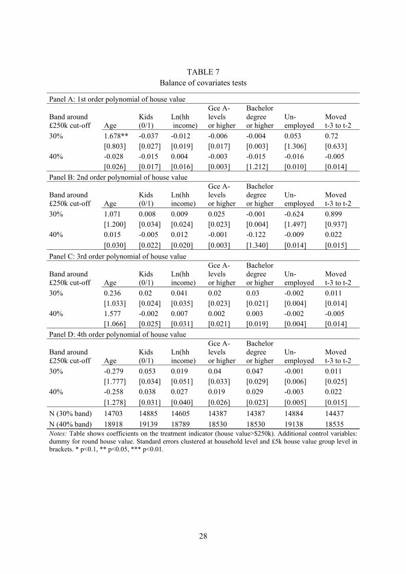
28  

TABLE 7 Balance of covariates tests

Panel A: 1st order polynomial of house value

Band around £250k cut-off Age

Kids (0/1)

Ln(hh income)

Gce A- levels or higher

Bachelor degree or higher

Un- employed

Moved t-3 to t-2

30% 1.678** -0.037 -0.012 -0.006 -0.004 0.053 0.72 [0.803] [0.027] [0.019] [0.017] [0.003] [1.306] [0.633]

40% -0.028 -0.015 0.004 -0.003 -0.015 -0.016 -0.005 [0.026] [0.017] [0.016] [0.003] [1.212] [0.010] [0.014]

Panel B: 2nd order polynomial of house value

Band around £250k cut-off Age

Kids (0/1)

Ln(hh income)

Gce A- levels or higher

Bachelor degree or higher

Un- employed

Moved t-3 to t-2

30% 1.071 0.008 0.009 0.025 -0.001 -0.624 0.899 [1.200] [0.034] [0.024] [0.023] [0.004] [1.497] [0.937]

40% 0.015 -0.005 0.012 -0.001 -0.122 -0.009 0.022

[0.030] [0.022] [0.020] [0.003] [1.340] [0.014] [0.015]

Panel C: 3rd order polynomial of house value

Band around £250k cut-off Age

Kids (0/1)

Ln(hh income)

Gce A- levels or higher

Bachelor degree or higher

Un- employed

Moved t-3 to t-2

30% 0.236 0.02 0.041 0.02 0.03 -0.002 0.011 [1.033] [0.024] [0.035] [0.023] [0.021] [0.004] [0.014]

40% 1.577 -0.002 0.007 0.002 0.003 -0.002 -0.005 [1.066] [0.025] [0.031] [0.021] [0.019] [0.004] [0.014]

Panel D: 4th order polynomial of house value

Band around £250k cut-off Age

Kids (0/1)

Ln(hh income)

Gce A- levels or higher

Bachelor degree or higher

Un- employed

Moved t-3 to t-2

30% -0.279 0.053 0.019 0.04 0.047 -0.001 0.011 [1.777] [0.034] [0.051] [0.033] [0.029] [0.006] [0.025]

40% -0.258 0.038 0.027 0.019 0.029 -0.003 0.022

[1.278] [0.031] [0.040] [0.026] [0.023] [0.005] [0.015]

N (30% band) 14703 14885 14605 14387 14387 14884 14437

N (40% band) 18918 19139 18789 18530 18530 19138 18535 Notes: Table shows coefficients on the treatment indicator (house value>$250k). Additional control variables: dummy for round house value. Standard errors clustered at household level and £5k house value group level in brackets. * p<0.1, ** p<0.05, *** p<0.01.  

29  

30  

TABLE 8 Stamp duty and mobility – Controls added

Panel A: 3rd order polynomial of house value

Band around All moves

Short moves

Long moves

Housing and area moves

Employment moves

Life event moves

£250k cut-off 30 % -0.024*** -0.032*** 0.008 -0.021*** 0.002 -0.006 N=14225

[0.010] [0.007] [0.007] [0.007] [0.002] [0.006] -5704 -14361 -16035 -16782 -49354 -21762

40 % -0.026*** -0.032*** 0.006 -0.020*** 0.002 -0.007 N=18296 [0.009] [0.006] [0.006] [0.007] [0.002] [0.007]

-6306 -16880 -20150 -20047 -61629 -25647

Panel B: 4th order polynomial of house value

Band around All moves

Short moves

Long moves

Housing and area moves

Employment moves

Life event moves

£250k cut-off 30 % -0.028** -0.042*** 0.014 -0.021** 0.002 -0.017* N=14225

[0.014] [0.010] [0.011] [0.010] [0.003] [0.010] -5703 -14364 -16036 -16782 -49364 -21768

40 % -0.026*** -0.037*** 0.012 -0.022*** 0.002 -0.006 N=18296 [0.011] [0.008] [0.009] [0.008] [0.003] [0.008]

-6312 -16879 -20152 -20051 -61629 -25647 Notes: Table shows coefficients on the treatment indicator (house value>$250k). Additional control variables: year dummies, dummy for round house value, age, household income, dummy for kids, 18 region dummies, dummy for GCE A-levels, dummy for bachelor degree or higher and dummy for unemployed, dummy for moved between t-3 and t-2. Standard errors clustered at household level and £5k house value group level in brackets. * p<0.1, ** p<0.05, *** p<0.01. Akaike Information Criterion is shown in italics. 

TABLE 9 Welfare effects of the stamp duty increase from 1% to 3%

(the ratio of welfare loss to revenue increase)

Average utility loss per move (proportion of house value)

Impact of stamp duty increase on mobility β = -0.017 β = -0.026 β = -0.035

λ = 0.02 (uniform distribution) 0.479 0.839 1.321

λ = 0.01 (lower bound) 0.239 0.419 0.660

31  

Figures

FIGURE 1 Distribution of self-assessed house values in 2006 (excluding recent movers)

32  

FIGURE 2 Mobility and self-assessed house values 

Notes: Circles indicate mobility rate in £10k bins after controlling for round values divisible by £50k. The size of the circle is proportionate to the number of observations in the bin. The line shows the fit of a regression of a mover dummy on a dummy for self-assessed house value above £250k, a 4th order polynomial for the whole range and a dummy for round values divisible by £50k. The gray area is the 95 % confidence interval.

33  

FIGURE 3 Placebo tests with artificial cut-offs

(Specification: 30% band and 3rd order polynomial, Outcome: all moves)

Notes: The figure shows the coefficients on placebo treatment dummies and the attached 95 percent confidence intervals for artificial cut-offs at £5k intervals between £150k and £350k (blue circles) where stamp duty does not change, and the actual cut-off at £250k (red square) where the stamp duty jumps from 1% to 3%. The sample used in each regression includes house values +/- 30% of the respective cut-off value. Controls include a 3rd order polynomial of house value and a dummy for round values divisible by £50k.

‐0.1

‐0.08

‐0.06

‐0.04

‐0.02

0

0.02

0.04

0.06

0.08

0.1

150 175 200 225 250 275 300 325 350

Coefficient on the treatment indicator 

Placebo cut‐off (£ 1000)

Placebo Actual

34  

FIGURE 4 Placebo tests with artificial cut-offs

(Specification: 40% band and 4th order polynomial, Outcome: all moves)

Notes: The figure shows the coefficients on placebo treatments and the attached 95 percent confidence intervals for artificial cut-offs at £5k intervals between £150k and £350k (blue circles), and the actual cut-off at £250k (red square). The sample used in each regression includes house values +/- 40% of the respective cut-off value. Controls include a 4th order polynomial of house value and a dummy for round values divisible by £50k.

‐0.1

‐0.08

‐0.06

‐0.04

‐0.02

0

0.02

0.04

0.06

0.08

0.1

150 175 200 225 250 275 300 325 350

Coefficient on the treatment indicator

Placebo cut‐off (£ 1000)

Placebo Actual

35  

Appendix

APPENDIX TABLE A1 Construction of type of move variables

Job-related moves Housing- and area-

related moves Major life event-

related moves

Did you move for reasons that were wholly or partly to do with your own job, or employment opportunities?

YES NO NO and/or and and

What were your (other) main reasons for moving?

Job reason, self Larger accommodation Move in with partner Job reason, other Smaller accommodation Split from partner Own accommodation Move in with family (If other than job reasons given, Buy accommodation Move from family not included in any category) No stairs Move in with friend

Another type Closer to family or friends Disliked previous accommodation Move to college Better accommodation Left college Privacy Retirement Wants change Evicted, repossessed Disliked isolation Health reasons To rural environment From rural environment Traffic Area unsafe Noise Area unfriendly To specific place

Disliked area

36  

APPENDIX TABLE A2

Balancing tests for predicted mobility

Dependent variable: Predicted moving probability (0/1)

Band around Order of polynomial of house value

£250k cut-off 1st 2nd 3rd 4th N 20 % -0.002 -0.002 -0.006 -0.006 6553

[0.004] [0.004] [0.005] [0.005]

-14830 -14829 -14829 -14829

30 % -0.002* -0.003 -0.002 -0.002 14406 [0.001] [0.002] [0.002] [0.003] -65074 -65073 -65074 -65074

40 % -0.001 -0.003 -0.004** -0.001 18534 [0.002] [0.002] [0.002] [0.002]

-79025 -79034 -79048 -79060 Notes: Table shows coefficients on the treatment indicator (house value>$250k). Additional control variables: dummy for round house value. Standard errors clustered at household level and £5k house value group level in brackets. * p<0.1, ** p<0.05, *** p<0.01. Akaike Information Criterion is shown in italics.

37  

APPENDIX TABLE A3 Stamp duty and mobility – Sample includes

only households saying they would like to move

Panel A: 3rd order polynomial of house value

Band around All moves

Short moves

Long moves

Housing and area moves

Employment moves

Life event moves

£250k cut-off 30 % -0.076* -0.119*** 0.043 -0.054** -0.003 -0.023 N=

2966 [0.043] [0.024] [0.029] [0.025] [0.006] [0.026] 1598 -39 -510 -103 -7938 -1408

40 % -0.101** -0.112*** 0.011 -0.068*** -0.007 -0.037 N= 4025 [0.040] [0.022] [0.029] [0.024] [0.006] [0.026]

2376 193 -498 133 -9750 -1507

Panel B: 4th order polynomial of house value

Band around All moves

Short moves

Long moves

Housing and area moves

Employment moves

Life event moves

£250k cut-off 30 % -0.034 -0.150*** 0.117*** -0.055 -0.001 -0.044 N=

2966 [0.049] [0.034] [0.040] [0.034] [0.007] [0.033] 1598 -39 -522 -101 -7936 -1408

40 % -0.06 -0.125*** 0.065** -0.054* -0.003 -0.019 N= 4025 [0.040] [0.025] [0.033] [0.029] [0.008] [0.029]

2374 195 -509 135 -9749 -1507 Notes: Table shows coefficients on the treatment indicator (house value>$250k). Additional control variables: dummy for round house value divisible by £50k. Standard errors clustered at household level in brackets. * p<0.1, ** p<0.05, *** p<0.01. Akaike Information Criterion is shown in italics.

38  

APPENDIX TABLE A4 Stamp duty and mobility – Coefficients on nth order polynomials

allowed to vary on different sides of cut-off

Panel A: 1st order polynomial of house value

Band around All Moves

Short Moves

Long Moves

Housing and area moves

Employment moves

Life event moves

£250k cut-off 30 % -0.037*** -0.041*** 0.004 -0.027*** 0.000 -0.003 N=

15322 [0.011] [0.007] [0.008] [0.008] [0.003] [0.007] -6041 -15403 -17260 -18494 -52609 -23742

40 % -0.019* -0.026*** 0.007 -0.015* 0.001 -0.004 N= 19701 [0.010] [0.007] [0.007] [0.008] [0.002] [0.006]

-6532 -18209 -21339 -21843 -63949 -27983

Panel B: 2nd order polynomial of house value

Band around All Moves

Short Moves

Long Moves

Housing and area moves

Employment moves

Life event moves

£250k cut-off 30 % -0.016 -0.035*** 0.020 -0.018 0.001 -0.012 N=

15322 [0.018] [0.011] [0.014] [0.011] [0.004] [0.009] -6041 -15399 -17261 -18491 -52607 -23741

40 % -0.037** -0.049*** 0.012 -0.030*** 0.000 -0.006 N= 19701 [0.015] [0.009] [0.012] [0.009] [0.003] [0.008]

-6537 -18221 -21336 -21852 -63945 -27985

Panel B: 3rd order polynomial of house value

Band around All Moves

Short Moves

Long Moves

Housing and area moves

Employment moves

Life event moves

£250k cut-off 30 % -0.029 -0.024 -0.005 -0.039*** -0.006 0.000 N=

15322 [0.026] [0.016] [0.022] [0.014] [0.007] [0.013] -6050 -15409 -17262 -18493 -52606 -23762

40 % -0.019 -0.027*** 0.008 -0.024* -0.003 -0.012 N= 19701 [0.024] [0.014] [0.019] [0.012] [0.006] [0.013]

-6537 -18221 -21334 -21851 -63943 -27982 Notes: Table shows coefficients on the treatment indicator (house value>$250k). Additional control variables: dummy for round house value divisible by £50k. Standard errors clustered at household level in brackets. * p<0.1, ** p<0.05, *** p<0.01. Akaike Information Criterion is shown in italics.

39  

APPENDIX FIGURE A1 Predicted mobility and self-assessed house values

Notes: Circles indicate predicted mobility rate in £10k bins from a regression of a mover dummy on the following covariates: age (and its square), dummy for kids, log of household income (and its square), dummy for GCE A-levels, dummy for bachelor degree or higher, dummy for unemployed and dummy for moved between t-3 and t-2. The size of circle is proportionate to the number of observations in the bin. The line indicates the fit of a regression of predicted mobility on a dummy for self-assessed house value above £250k, a 4th order polynomial of house value and a dummy for round values divisible by £50k. The gray area is the 95 % confidence interval.

40  

APPENDIX FIGURE A2 Robustness of results on long/short distance mobility to definition of long/short distance

moves (Specification: 40% band and 4th order polynomial)

Notes: The figure shows the coefficient on the treatment indicator and the attached 95 percent confidence interval for long distance mobility (red dots) and short distance mobility (blue dots) when we vary the definition of long/short distance between 5 and 15 kilometers., using a 40 percent band around the cut-off and a 4th order polynomial of house value.

‐0.06

‐0.05

‐0.04

‐0.03

‐0.02

‐0.01

0

0.01

0.02

0.03

4 6 8 10 12 14 16

Estimated effect of stam

p duty

Defintion of short/long distance  move (km)

Short distance mobility Long distance mobility