TRANSDUCTION BASED APPROACHES FOR DATASET SHIFT …
98
Graduate Program in Electrical Engineering TRANSDUCTION BASED APPROACHES FOR DATASET SHIFT PROBLEMS CARLA CALDEIRA TAKAHASHI 2019
Transcript of TRANSDUCTION BASED APPROACHES FOR DATASET SHIFT …

Graduate Program in Electrical Engineering
T R A N S D U C T I O N B A S E D
A P P R O AC H E S F O R DATA S E T S H I F T
P R O B L E M SC A R L A C A L D E I R A TA K A H A S H I
2019

Federal university of Minas GeraisSchool of Engineering
Graduate Program in Electrical Engineering
Transduction Based Approaches for Dataset Shift Problems:
Carla Caldeira Takahashi
Advisor: Prof. Dr. Antônio de Pádua Braga
Belo Horizonte, Brazil
2019

Carla Caldeira Takahashi: Transduction Based Approaches for Dataset Shift Problems, c©2019

Nous ne pouvons pas construire un monde
meilleur sans améliorer les individus. Dans
ce but, chacun de nous doit travailler à son
propre perfectionnement, tout en acceptant
dans la vie générale de l’Humanité sa part de
responsabilités.
Marie Curie, in Madame Curie, by Ève Curie
(1937)

A B S T R AC T
Dataset Drift problems occur in every field that extract or adjust models from data. It is named drift
the phenomena which causes the training and testing datasets to differ, and may also appear at any time
during the model real application. In this context, approaches using Transductive learning were proposed
to solve classification problems under some Dataset Drift scenarios. Two strategies were defined, and
present satisfactory results with some limitations. The first one is based on an Essentially Transductive
Approach that uses genetic algorithm to optimize data entropy. The other one is a strategy oriented
to two-dimensional spatial datasets based on Gabriel Graphs for the estimation of Gaussian Mixture
Models. However, the correct analysis if the model under a drift is not systematically performed, thus
the experimentation of the methods was done with study cases.

R E S U M O
O problema do Dataset Drift ocorre em toda e qualquer área que utilize dados para criar ou ajustar
modelos. É chamado de drift o fenômeno que faz com que haja alguma diferença entre os dados de
treinamento e os de teste, além de se manisfestar em qualquer momento no ambiente de aplicação real
do modelo. Nesse contexto são sugeridas abordagens utilizando aprendizado transdutivo para lidar com
o Dataset Drift. Duas estratégias foram definidas e apresentam resultados satisfatórios com algumas
limitações. A primeira é baseada em uma Abordagem Essencialmente Transdutiva que utiliza um algo-
ritmo genético para a otimização da entropia dos dados. A outra é uma estratégia orientada a problemas
espaciais bidimensionais, baseada em Grafos de Gabriel para a estimação de Modelos de Mistura Gaus-
siana. No entanto, a análise da qualidade dos modelos perante a presença do drift ainda não é realizada
de forma sistemática, dessa forma os experimentos foram feitos com estudos de caso.

C O N T E N T S
1 I N T R O D U C T I O N 13
2 L I T E R AT U R E R E V I E W 18
2.1 Dataset Shift . . . . . . . . . . . . . . . . . . . . . . . . . . . . . . . . . . . . . . . . . 19
2.1.1 Types of Dataset Shift . . . . . . . . . . . . . . . . . . . . . . . . . . . . . . . 21
2.1.2 Dataset Shift Characteristics in Time . . . . . . . . . . . . . . . . . . . . . . . . 29
2.1.3 Causes of Dataset Shift . . . . . . . . . . . . . . . . . . . . . . . . . . . . . . . 32
2.1.4 Learning Strategies for Shifting Datasets . . . . . . . . . . . . . . . . . . . . . 38
2.1.5 Popular Approaches for Dataset Shifting Problems . . . . . . . . . . . . . . . . 41
2.2 Statistical Distributions Comparison . . . . . . . . . . . . . . . . . . . . . . . . . . . . 46
2.2.1 Dissimilarities and Similarities Measures . . . . . . . . . . . . . . . . . . . . . 46
2.3 Transductive Learning . . . . . . . . . . . . . . . . . . . . . . . . . . . . . . . . . . . 49
2.4 Gabriel Graphs Gaussian Mixture Models . . . . . . . . . . . . . . . . . . . . . . . . . 52
2.4.1 Gabriel Graphs . . . . . . . . . . . . . . . . . . . . . . . . . . . . . . . . . . . 53
2.4.2 Geometric Parametrization of Gaussian Mixture Models . . . . . . . . . . . . . 55
2.5 Spatial Clustering Based on Delaunay Triangulation . . . . . . . . . . . . . . . . . . . . 56
3 P R O P O S E D M E T H O D S 57
3.1 Essentially Transductive Learning with Genetic Optimization . . . . . . . . . . . . . . . 58
3.1.1 Minimizing Intra-Class Information Degeneration . . . . . . . . . . . . . . . . 59
3.1.2 Maximizing Inter-Class Information Degeneration . . . . . . . . . . . . . . . . 60
3.1.3 Implementation Aspects . . . . . . . . . . . . . . . . . . . . . . . . . . . . . . 60
3.2 Transductive Approach based on Gabriel Graphs . . . . . . . . . . . . . . . . . . . . . 63
3.2.1 Transductive Labelling . . . . . . . . . . . . . . . . . . . . . . . . . . . . . . . 63
3.2.2 Structural Classifier Selection . . . . . . . . . . . . . . . . . . . . . . . . . . . 64
4 E X P E R I M E N TA L D E S I G N 67
4.1 Genetic Essentially Transductive Learning Experimental Design . . . . . . . . . . . . . 68
4.1.1 Imbalanced Datasets . . . . . . . . . . . . . . . . . . . . . . . . . . . . . . . . 68
4.1.2 Dataset Drift . . . . . . . . . . . . . . . . . . . . . . . . . . . . . . . . . . . . 71
6

C O N T E N T S 7
4.2 Gabriel Graph Transductive Approach Experimental Design . . . . . . . . . . . . . . . 73
5 E X P E R I M E N TA L R E S U LT S 74
5.1 Genetic Essentially Transductive Learning Experiments Results . . . . . . . . . . . . . 75
5.1.1 Imbalanced Datasets . . . . . . . . . . . . . . . . . . . . . . . . . . . . . . . . 75
5.1.2 Dataset Drift . . . . . . . . . . . . . . . . . . . . . . . . . . . . . . . . . . . . 78
5.2 Gabriel Graph Transductive Approach Experimental Results . . . . . . . . . . . . . . . 79
5.2.1 Graphical Example . . . . . . . . . . . . . . . . . . . . . . . . . . . . . . . . . 79
5.2.2 Comparison with State of Art methods . . . . . . . . . . . . . . . . . . . . . . . 81
6 C O N C L U S I O N 84
References
1 B I B L I O G R A P H Y 88

L I S T O F F I G U R E S
Figure 2.1 Covariate Shift: Ptrain(y|x) = Ptest(y|x) and Ptrain(x) 6= Ptest(x), where the
distribution of class 0, P(x|y = 0)P(y = 0), is given in red and the distribution
of class 1,P(x|y = 1)P(y = 1), is given in blue. . . . . . . . . . . . . . . . . 22
Figure 2.2 Dataset with causal relation between x and y, in which training data are the
darker dots and testing data are the lighter ones. This variation in the abscissa
axis characterizes a covariate shift[77]. . . . . . . . . . . . . . . . . . . . . . . 23
Figure 2.3 Misspecified models caused by covariate shift[77], Here, darker dots are the
training set and the lighter ones are the test set. . . . . . . . . . . . . . . . . . 24
Figure 2.4 The distribution of each class differs greatly between training and testing. . . . 25
Figure 2.5 Prior Probability Shift: Ptrain(x|y = 0) = Ptest(x|y = 0) and Ptrain(x|y =
1) = Ptest(x|y = 1) but Ptrain(y = 0) 6= Ptest(y = 0) and Ptrain(y = 1) 6=
Ptest(y = 1). Here, the distribution of class 0, P(x|y = 0)P(y = 0), is given
in red and the distribution of class 1,P(x|y = 1)P(y = 1), is given in blue. . . 25
Figure 2.6 Graphical representation of prior probability shifts in datasets, where darker
dots are the training set, the lighter ones are the test set. [77] . . . . . . . . . . 26
Figure 2.7 The information distribution depends on the target value, characterizing prior-
probability shift. Here training data is represented by 2.7b and test data by 2.7c. 27
Figure 2.8 Concept Shift:Ptrain(x) = Ptest(x) but Ptrain(y|x) 6= Ptest(y|x) . . . . . . . . . 27
Figure 2.9 Graphical representation of real and virtual of covariate drifts. Here, circles
represent instances and different colours represent different classes.[36] . . . . 28
Figure 2.10 This is the graph of the speed of a three-phase electric motor. The training data
is the motor speed for a controlled training set-point. The orange data is the
motor working with a covariate shift, i.e. a shifted set-point. The red plot is the
output of the system for the same set-point as the training data but the motor
has a short-circuit phase fault . . . . . . . . . . . . . . . . . . . . . . . . . . . 29
Figure 2.11 Graphical representation different dataset shift behaviours in time [36]. . . . . . 30
Figure 2.12 Example of audio data collected indoors(red) and outdoors(blue), where street
noise had a expressive impact on the overall data. A machine trained for with
the indoor data should compensate possible background noise. . . . . . . . . . 30
8

L I S T O F F I G U R E S 9
Figure 2.13 Incremental Shift represented by pictures of a person in her infancy (Initial State
A), childhood, teenage and adulthood (Final State B), The L2 distance to the A
state was calculated with OpenFace[4]. . . . . . . . . . . . . . . . . . . . . . . 31
Figure 2.14 The selection variable s and its selection function given by the equiprobable
contour define which data are sampled [77]. Where darker dots are the train-
ing set, the lighter ones are the test set and the contour is the boundary of the
selection function. . . . . . . . . . . . . . . . . . . . . . . . . . . . . . . . . . 34
Figure 2.15 Dataset shift caused by class rebalance for a two class case example, where the
darker dots are training data and lighter ones are test data [77]. . . . . . . . . . 35
Figure 2.16 Projection of the features Albumin and Prothrombin Time from the Hepatitis
dataset. Class Live (green) has significantly more instances than class Die (red
in Fig 2.15a. The under sampling process dependent on values of other features,
such as Malaise, Age and Histology, resulted in the misspecified models in
2.15b, with the class contours significantly different. . . . . . . . . . . . . . . . 35
Figure 2.17 Representation of Domain Shift regarding the modelling structure and data dis-
tribution [77]. . . . . . . . . . . . . . . . . . . . . . . . . . . . . . . . . . . . 37
Figure 2.18 Representation of image capture problem where domain shift occurs due varia-
tion in camera settings. The plot displays the average luminance of the pictures
columnwise. The training data is in red and the test in blue. . . . . . . . . . . . 37
Figure 2.19 Active approaches use a change detector to inspect the inputs and/or classifica-
tion error over the labelled samples. The detector signs the adaptation mecha-
nism to update the classifier[25]. . . . . . . . . . . . . . . . . . . . . . . . . . 39
Figure 2.20 Learning model based on inductive inference, where a function that best ap-
proximates the unknown functional dependence is selected from the set of all
possible functions based on the given training data. . . . . . . . . . . . . . . . 49
Figure 2.21 Learning model based on transductive inference. A modified learning machine
takes both training and working sets as inputs, and the evaluator is only able to
estimate values on either of these sets. . . . . . . . . . . . . . . . . . . . . . . 51
Figure 2.22 Gabriel Graph based on Voronoi Diagram. (a) Voronoi diagram. (b) Voronoi
diagram dual graph. (c) Delaunay triangulation. (d) Pair of points from Voronoi
diagram with an edge of a Gabriel graph. . . . . . . . . . . . . . . . . . . . . 53

L I S T O F F I G U R E S 10
Figure 2.23 Visualization of the construction of a Gabriel Graph, in successive steps from
(a) to (h). The dots are the scattered vertexes while the edges in solid lines are
being creates. Each dashed circle represents the hypersphere of the criteria in
Eq. 36 . . . . . . . . . . . . . . . . . . . . . . . . . . . . . . . . . . . . . . . 54
Figure 4.1 Diagram of the Transductive Experiment . . . . . . . . . . . . . . . . . . . . . 69
Figure 4.2 Diagram of the Transductive Experiment . . . . . . . . . . . . . . . . . . . . . 71
Figure 4.3 Graphical representation of the Two Moon Dataset with Covariate Shift. . . . . 72
Figure 4.4 Diagram of the Transductive Experiment . . . . . . . . . . . . . . . . . . . . . 73
Figure 5.1 Accuracy comparison of the ETC with Inter-Class maximization, SVM and the
TSVM. . . . . . . . . . . . . . . . . . . . . . . . . . . . . . . . . . . . . . . 75
Figure 5.2 Normalized Accuracy of SVM, TSVM and ETL for hepatitis, Pima Indian
diabetes, Wisconsin breast cancer and two moons datasets, with DL = 10
and 5. The balance varies from 0% (only positive class) to 100% (only negative
class) by 10% and 20% for DL = 10 and 5, respectively. . . . . . . . . . . . . 76
Figure 5.3 Normalized GMEAN of SVM, TSVM and ETL for hepatitis,Pima Indian di-
abetes, Wisconsin breast cancer and two moons benchmark datasets, with
DL equal to 10 and DL equal to 5. The balance varies from 0% (data only from
positive class) to 100% (data only from positive class) by 10% for DL = 10
and by 20% for DL = 5. . . . . . . . . . . . . . . . . . . . . . . . . . . . . . 76
Figure 5.4 Pairwise Wilcoxon Rank Sum Test with 95% confidence level of SVM, TSVM
and ETL for hepatitis, Pima Indian diabetes, Wisconsin breast cancer and
two moons benchmark datasets. Results after 90 executions of each combina-
tion with distinct unbiased samplings for DL equal to 10 and after 40 executions
for DL equal to 5. . . . . . . . . . . . . . . . . . . . . . . . . . . . . . . . . . 77
Figure 5.5 Pairwise Wilcoxon Rank Sum Test with 95% confidence level of SVM, TSVM
and ETL for Two Moons, Circle and Sinusoidal benchmark datasets with
Drift. Results after 30 executions of each. . . . . . . . . . . . . . . . . . . . . 78
Figure 5.6 Transductive Resulting Graph . . . . . . . . . . . . . . . . . . . . . . . . . . . 79
Figure 5.7 Spatial Cluster for Working data . . . . . . . . . . . . . . . . . . . . . . . . . 80
Figure 5.8 Spatial Cluster for Unsupervised data . . . . . . . . . . . . . . . . . . . . . . . 80
Figure 5.9 Transductive Labels with resulting Graph . . . . . . . . . . . . . . . . . . . . 80
Figure 5.10 The classification of the Two Moon Dataset performed by the proposed method
in comparison to SVM Classifier, both using the Transductive Labeling as input 81

L I S T O F F I G U R E S 11
Figure 5.11 The classification of the Circle Dataset performed by the proposed method in
comparison to SVM Classifier, both using the Transductive Labeling as input . 81
Figure 5.12 Accuracy comparison of the Transductive Gabriel Graph with State-of-Art Meth-
ods, using Transductive Labelling and Not using it, and the Transductive SVM. 82
Figure 5.13 Computational Training and Prediction Time for the Transductive Gabriel Graph
compared to State-of-Art Methods, using Transductive Labelling and Not using
it, and Transductive SVM . . . . . . . . . . . . . . . . . . . . . . . . . . . . . 83

L I S T O F TA B L E S
Table 4.1 Datasets Description . . . . . . . . . . . . . . . . . . . . . . . . . . . . . . . 70
Table 4.2 Description of the datasets with concept drift . . . . . . . . . . . . . . . . . . . 72
12

1 I N T R O D U C T I O N
The future is already here - it’s just not very
evenly distributed.
Willian Gibson, "The Science in Science
Fiction" on Talk of the Nation, NPR (30
November 1999, Timecode 11:55)
13

I N T R O D U C T I O N 14
Data, at present, is generated in great amounts and with great speed. The systems which generate these
data have become complex in such way that their modelling require advanced techniques and methodolo-
gies that extract information from data itself. Strategies to learn from data are present in a large variety
of research fields such as Machine Learning, Data Mining, Statistics, System Identification, among oth-
ers, and have application in vast range of problems including biomedical, financial, information science,
ecology, industrial automatic control, computer vision, game development and entertainment. In this
context, the importance of correct information extraction from data is widely related to the efficiency of
the final application, which could be the diagnosis of a certain disease, credit approval system, optimal
automation of an industrial plant, visual recognitions for video game consoles such as Kinect, etc.
Machine Learning methods allows automated models building, with the knowledge extracted directly
from data. In this science field, the machine, or computer, is able to learn information through data
analysis, unveiling hidden insights, which could not be immediately perceived, without necessarily being
explicitly programmed for that. Usually, in this field, it is desired to generate a model that is capable of
imitating an unknown system with the objective of: (a) label unknown data as the original system would,
which defines classification models; (b) return de output for a given input according to the original system
function, which occurs in function regression or time series prediction; or (c) grouping data according to
its intrinsic characteristics, which is performed by unsupervised clustering algorithms. There are several
methods and strategies for each of these types of machine learning algorithms, nevertheless all of them
have as a common characteristic the fact that they all extract information from data and create stochastic
models. Additionally, several other fields extract information from data, although each one have different
objectives to reach.
Learning from data, either in Machine Learning or any other field, has a number of particularities that
must be properly managed regarding its stochastic characteristics. As data itself, even if generated from
the same system, tends not to be stationary, the modelling of the system needs strategies to either adapt to
data as it is provided or to be robust to any variations of the data, whatsoever they may be. In real world
scenarios, non-stationarity is an issue which occurs naturally in most of systems, intrinsic characteristics
or even external factor might change its behaviour and, thus, the data it generates. Considering modelling
strategies that uses data to generate its models, this variation implies that the model will eventually
become inadequate.
In a broad definition, the phenomena where the data generated by any system changes, either slowly or
abruptly, is named Dataset Shift. This becomes a serious issue since the model created for these systems
become unfit for its actual application. In Machine Learning contexts, some initial data is required to
create the model that will be applied, later, to the system, either to classify new data, cluster new sets or
mimic the system output values according to its function regression. The model is then, created according

I N T R O D U C T I O N 15
to a very specific set of data and, if the application, or testing, data was actually generated differently the
classification, clustering or regression are simply wrong and may not lead to the correct outputs.
Dataset Drifting problem is a serious issue in several applications, since it causes models response to
degrade in the application space, not because of an internal degeneration, but due to a modification in
the input and output relation. Despite the existence of robust and adaptive methods, which work well
for some specific scenarios, the drifting context more comprehensive then noise issues or an systematic
input variation. More forebodingly, dataset drift might occur in data in unexpected manners but, still,
the models should be able to extract the necessary information. It is precisely the nature of this needed
information that defines if a simpler robust or adaptive is enough or a more complex approach for dataset
drift is necessary. Defining and setting the modelling methodology depends on what is needed to be
known and the drifts affects it.
The dataset shifting may occur for several reasons, the system could be non-stationary and gradually
suffers changes in time, which is common in industrial plants where there are sensors and actuators
degradation. Another situations occurs when the training data is obtained in a context different from
the actual application data, for instance an image recognition system which was trained with different
lighting conditions from the application. The speed of the shift also raises an important issue, since it
interferes in the difficulty of actually detecting or adapting to it. When the data suffers a fast unexpected
change it is called abrupt and a tendency which slowly changes data is named a gradual shift, they can
both occur in the same system simultaneously, for instance a greenhouse or a clean room temperature
control system has to adapt to the weather of all the seasons of the year, which gradually raises and lowers
the temperature consisting in a gradual shift, however any possible fault on a fan or air conditioning
would be an abrupt shift that should be considered in the system.
Despite all of the reasons and forms of shifts, they can be defined statistically according to its distri-
bution characteristics. Thus, a systematic approach for detecting and adapting or disregarding it could
be properly designed. This work premise is that, with an appropriate employment of statistical data
distribution testing and statistical model adaptation, the dataset shift issue could be minimized, as an
intermediate stage, for different modelling strategies and methods from different fields.
Given that different types of dataset shifts can be categorized according to their effects over the data
statistical distributions, in disregard of the reason or the velocity of the shift, not only the occurrence of
a given shift can be detected but also the identification of which type of shift can performed. There is a
consequential relation between shift types and their reason for appearing, thus the identification of shift
lead to the unveiling of its possible causes and, hence, might allow the correction, or the control, of the
shift itself instead of its consequences.

I N T R O D U C T I O N 16
Probability density estimation methods define the characteristics and parameters of a dataset distribu-
tions adjusting it to a known statistical distribution type, thereby it is possible, for instance to define the
dataset distribution in different points and assert whether they are similar or if a shift occurred. Nonethe-
less, the comparison between distributions is not simple, and recognizing the specific difference between
them might not even be possible, however measuring, in a quantitative manner, how similar they are can
be promptly solved. The measure of the distance between two distributions can be achieved by their
dissimilarity, analogously the similarity can be defined according to the distributions proximity.
Despite the categorization of the causes that lead to Dataset Shifting, the shift can be also defined
according to its manifestation over the data statistical distribution and its effect on the model output,
disregarding its specific cause. This allows particular methods and techniques to perform reasonably
well for several types of Dataset Shifts even though their cause might differ. It can, then, be said that
the shift reason is transparent to the model as it receives only raw data and perceives only the statistical
information observable in it. In this context, the principal characteristic of the Dataset Shift is whether
it occurs abruptly or gradually. Expressly, if changes on data distributions occur very fast in specific
instants, thus being abrupt, or if it is a slow and constant deviation that affects data gradually.
However, there remains the need to define systematically how well the selected model is able to per-
form in different Dataset Shift conditions. Considering this, the main objective of this work is to delineate
a series of procedures to test whether a model of interest behave under data shifting and measure the effect
of different types of shifts on the models output. In this matter, a systematic quantitative measurement of
the effects of the shift on the model enables a efficient analysis of the model components which, in fact,
interfere in the performance of the model. For instance, it is possible to define if either the modelling
methodology, or the metrics used, had any significance on the results achieved by the model. This topic
does not have conclusive nor significant approaches in the literature, thus in this work it is proposed an
strategy to systematically analyse models performance when subject to dataset drifting scenarios, based
on stability criteria.
Considering the characteristics of the drifting problem, it is expected that semi-supervised and trans-
ductive approaches that uses both the training labelled and unlabelled testing or working datasets might
lead to improved models. In this context, a transductive method in which a model is defined to work
specifically in the current working set. In contrast to the traditional inductive approach, a general model
is not generated from the particular testing data and for each working set a new model is defined. Thereby,
a transductive method with statistical similarity metrics was implemented envisaging an improved per-
formance in dataset drifting scenarios.
This thesis will be divided in six chapters, in which the first one is this introduction and the next
chapters will have the following structure: the second chapter is a literature survey and will include an

I N T R O D U C T I O N 17
comprehensive presentation of the Dataset Shift issues and approaches in literature and the necessary
informations about the methods employed in this work; chapter 3 consists in the description and justifica-
tions of the approaches used to design the proposed methods for solving classification with data drifting;
4 chapter describes the proposed analysis strategies for experimental methodology; the fifth chapter con-
tains results obtained by the test designed in previous chapters and also provides valid statistical analysis
of results; in the last chapter, are the conclusions of this work and the future work.

2 L I T E R AT U R E R E V I E W
Time is not a line but a dimension, like the
dimensions of space
Margaret Atwood, Cat’s eye
18

DATA S E T S H I F T 19
2.1 DATA S E T S H I F T
The formalization of machine learning methods according to statistical premisses and formulations is of
great importance because it allows definitions of learning quality and risk. While stochastic methods,
as most of Machine Learning methods are, can easily fall under computational methods with perfor-
mance empirically proven, the incorporation of statistical learning theories to the field, for instance with
[100], allows, then, theoretical foundations and analysis standardization. The risk limits concepts, can
be used both as model training parameters or as criteria for model selection. This relation with statistical
fundamentals require the statistical premisses to be met as well, however in real-world problems, these
dependences might not be true as the datasets might not be easily defined, for instance the data distribu-
tion is commonly not defined and sometimes can not be well estimated. In this context, an issue that has
been studied in recent years is the Dataset Shift, which defines the phenomena when the training dataset
differs from the testing or application datasets.
Regarding learning problems, the main objective of function estimation is selecting a model capable
of producing correctly the expected responses of a given system, usually named supervisor, according to
specified inputs. Which is done, however, having as reference a limited set of examples of the supervisor
behaviour [9], thus, the necessary and available components for modelling are:
1. A generator of random vectors x, defined by a fixed and unknown distribution P(x).
2. A supervisor which generates an output y given an input x, according to a fixed and unknown
conditional distribution function P(y|x);
3. A machine that implements a set of functions f (x, w), w ∈ Λ.
A machine learning problem consists in a correct function selection, within the set f (x, w), w ∈
Λ, that more accurately imitates the supervisor behaviour. In this context, the training set should be
composed of independent identically distributed(i.i.d.) samples according to the distribution P(x, y) =
P(x)P(y|x) and should be sufficiently large to guarantee data representativeness.
The risk and loss functions relation is measured according to differences between the supervisor re-
sponse - y given x - and results provided by the learning machine - f (x, w). Risk limits allow a consistent
analysis of the learning premisses and, thus, allow several statistical learning method, at some degree,
to be primarily assessed by a theoretical criteria. The real risk functional R(w) can be represented by
Equation 1. [102, 77, 67]
R(w) =∫
L(y, f (x, w))p(x, y)dxdy (1)
in which L(y, f (x, w)) is a loss function or discrepancy, the approximation function is f (x, w), and
(x, y) are pairs of inputs and outputs that must be completely described by a model. The joint probability

DATA S E T S H I F T 20
density function (pdf) given by p(x, y) should be known a priori. However, since the joint probability
density function is usually unknown and only a limited set of input/output pairs (x, y) is actually available
for evaluation, it is, then, necessary using an empirical risk function.
Furthermore, it exists another important reservation regarding PDFs used by machine learning model
estimators. In real-world problems, training data and test data densities might significantly differ. Which
characterizes a set of issues observed in machine learning and data mining named Dataset Shift. In
this context, it is possible to notice a significant limitation in methods which premises consider training
and test data to be i.i.d.. Breaking such premise imply in creating a model with a training set which
is not representative of the actual testing data and, thus, the machine itself is not adequate for the final
application [77, 67].
When considered the empirical risk of the Equation 2, proposed by [38], it is possible to define the
sampling error and the approximation error according to the Equation 3. In this case, the Dataset shift
should cause a distortion in the expected value E [y|x]. Hence, it is expected a deterioration of the
sampling and approximation errors.
Remp =1N
N
∑i=1
(yi − f (xi, w))2 (2)
E[(y− f (x, w))2] = E
[(y− E [y|x])2]+ E
[( f (x, w)− E [y|x])2] (3)
in which the first term, given by E[(y− E [y|x])2], is the sampling error and the second one, E
[( f (x, w)− E [y|x])2],
represents the approximation error.
In case there is a shift in p(y, x) there will be also a shift in the expected value of y, E [y|x], and
therefore, a degradation in sampling and approximation errors given by Equation 3. This situation will
happen when Ptrain(y, x) 6= Ptest(y, x) [77, 67] as a result of dataset shift. Considering that the system
is stationary, so P(y|x) does not change, a shift in P(y, x) can only be due to Ptrain(x) 6= Ptest(x),
characterized by a dataset shift, due to Equation 4.
P(y, x) = P(y|x)P(x) (4)
There are several types of Dataset Shift which can be defined according to the differences between
Ptrain(y|x) and Ptest(y|x) or between Ptrain(x) and Ptest(x) [67]. Other forms of “shift” might be related
to the differences in mechanisms which causes differences in the data, for instance: the source that
generated the training and test data might be slightly different, even if the data generated are intended
to be the same; the data domain could have its significance or interpretation changed when the context
changes from training to testing; the sampling my not be representative of the overall dataset; or even the
class imbalance problem can be considered a type of dataset shift [77].

DATA S E T S H I F T 21
One important observation regarding the study of Dataset Shift is related to its nomenclature, there is
a lack of agreement on names and terms used to appoint the same problems. In the machine learning
context, Dataset Shift was widespread by [77]. However, other therms, such as concept drift, concept
shift, data fracture, reject inference, among others, are used in different areas, as Statistics and Data
Mining, to denominate very similar or even the same class of problems. Therefore, achieving a complete
and extensive bibliographic review is rather overstraining [67].
The matter of a better agreement between the models, obtained through machine learning, and the real
problems is of great importance on the field of computer intelligence, since it allows not only a better
understanding of the real-world but also increases the control possibilities for these real systems. In the
real-world the environment and the time are non-stationary, thus the Dataset Shift is natural and is present
in several applications. However, in the Machine Learning field this subject has several limitations, for
instance, the detection and automatic classification of the different types of shift that may appear in a
problem is understudied, on the same context the methods that can deal simultaneously with more than
one shift are very rare.
2.1.1 Types of Dataset Shift
The dataset shifting is a general problem that may affect several types of data very differently. Strictly,
drifting occurs when the model training data form and intensity differ from the data that is actually
used during the model testing or its real employment. More directly, shifting is considered when the
phenomena that generates data undergoes some change in time.
The difference in the data distribution can unfold in very distinct manners, for instance, two different
density functions can show a distribution of the same type but with other coefficients, or the distribution
average and dispersion might be equivalent but the shape of the distribution could differ. In this context,
a variety of different shifts exist and have particular characteristics, usually three categories are defined:
covariate shift, prior-probability shift and concept shift.[82]
Covariate Shift
Covariate is a designation of the explanatory variable x. When the covariates future values are different
from past observations, it occurs a specific type of dataset shift, named Independent Covariate Shift or
simply Covariate Shift [90, 86]. This type of shifting occurs when only the distribution of x suffers some
variation, and all the other probabilities are kept equal, thus, according to Equation 4, Ptrain(y|x) =
Ptest(y|x) but Ptrain(x) 6= Ptest(x) As seen in Fig. 2.1, the relation between the target y and the covariate
x remains the same for both classes, but the distribution of de covariate P(x) changes. [86, 90, 77, 67].

DATA S E T S H I F T 22
In a streaming scenario this change could occur in any given time after the training, which was per-
formed in a reference time instant T. Thus the covariate shift occurs when it is perceived a change
in sampled data distribution between two consecutive time instants Pt−T(y|x) = Pt+1−T(y|x) but
Pt−T(x) 6= Pt+1−T(x) [25].
This mismatch is very common and is considered a fundamental form of Dataset Shift. It could be
said that it occurs when the mechanism that generates the data suffers some type of change in P(x)
between the training moment and the testing. Therefore it has a strong relation with time series predic-
tion problems. In real-world prediction problems, it is common that the mechanism that generates data
suffer changes in time, thus modifying the covariate density. However, it is not as likely that the phenom-
ena which produces the output given the input, the conditional probability P(y|x), suffer such changes.
Moreover, simple survey experiments tend to also show this sort of issue, since Ptrain(x) is determined
by sampling schemes and Ptest(x) is set by the population [77, 86].
0−a a
b2
b
x
Ptrain(x)Training Set
0−a a
b2
b
x
Ptest(x) Test Set
Figure 2.1: Covariate Shift: Ptrain(y|x) = Ptest(y|x) and Ptrain(x) 6= Ptest(x), where the distribution of class 0,
P(x|y = 0)P(y = 0), is given in red and the distribution of class 1,P(x|y = 1)P(y = 1), is given
in blue.
The covariate shift can be understood as a causal model where the covariate x value has influence on
the distribution of the targets y. In this case the prediction function and the noise model for the training
and testing data, but the typical position of the data provided during the training is different from that
applied to the tests. In figure 2.2, it is illustrated a causal model which training data are the dark dots and
the test data are the lighter ones. In this example the principal data generating function is basically the
same, but the covariate, x, position of the training data is different from the position of the testing data,
which would lead to very different estimated models.
Referring to eq. 1 it is straight forward that the risk changes with covariate shift since the integration
of the loss function L is performed with respect to a different portion of the input space. Let the model

DATA S E T S H I F T 23
risk be calculated over m different datasets, which allows it to be understood as a random variable R,
with mean and variance:
E [R] = E[(y− f (x, w))2] = m− 1
mµ2 (5)
var(R) = var[(y− f (x, w))2] = (m− 1)2
m3 µ4 −(m− 1)(m− 3)
m3 µ22 (6)
where
µn =∫ ∞
−∞(y− f (x, w))ndP(x, y) (7)
The integral of the power of the residual is performed with respect to the probability density, which, in
the case of covariate shift, is understood as P(x, y) = P(y|x)/P(x). Thus, the risk expected value and
variance might converge to a different value, due to their dependence to the PDF of x. Furthermore, in
shift problems, the model might not be well defined for the input xtest, causing the loss function results
to be unbounded and resulting in a larger variance.
y
x
Figure 2.2: Dataset with causal relation between x and y, in which training data are the darker dots and testing
data are the lighter ones. This variation in the abscissa axis characterizes a covariate shift[77].
In this context, estimating a linear global model according to the training set would result in a very
poor descriptor of the overall data, specially the test set. As seen in Figure 2.3a, the global estimation
with a linear model of the dark dots training data, represented by the dashed line, is a poor fit for the
overall data. Meanwhile, the linear local fits of the testing data, represented by the dashed lines in
2.3b, comprises of a completely different linear model. Shifts in the position of covariates in the input
domain could lead to different models, since data might be restricted to a limited space in the domain.
For instance, if the two dark dots farther left did not exist, the third local model would not exist as is.
Nonetheless, a global model based on local linear models, here, still leads to a better estimation. Thus, in
such cases, the local estimation of multiple models in the function domain could minimize error caused
by shifts in the covariate placement.
Misspecified models occur when the covariate used for training the model are not representative of the
testing set, furthermore, even if the models selected may not usually be completely representative of the
global original system, it is possible to select a local model suitable for the testing data if the right region
of the system domain is chosen. As seen in Figure 2.3, the sinusoidal function is not correctly defined by
the model in 2.3a, even with data distributed in all of its domain because a linear model is a very poor fit.

DATA S E T S H I F T 24
However, even a linear fit would create an appropriate model to predict the test data if just the covariates
in the correct range were used [77].
y
x
(a) The dashed line represents a global estimation
of a linear model, and the solid line represents
the causal generating function.
y
x
(b) Global model based on local linear models is
shown in the dashed line, and the solid line is
the representation of the generating function.
Figure 2.3: Misspecified models caused by covariate shift[77], Here, darker dots are the training set and the
lighter ones are the test set.
A typical example of covariate shift is its occurrence in the diagnosis of an individual future diseases
given one’s lifestyle. If someone has a drastic lifestyle change, it is possible that one’s risk of developing
certain diseases also change, however the probability that drives the development of these diseases within
the population itself does not change. For instance, if a man becomes less sedentary it is more likely that
his risk of developing a cardiovascular condition decreases, however the risk for sedentary people in
general of developing such diseases does not change. Similarly, a health condition survey done within an
university campus would not reflect the health status of the country population in general, since students
tend to be in a healthier age range [77].
Brain-Computer Interfaces (BCIs) based in electroencephalograms (EEG) are another typical example
often associated with covariate shift. In these systems, electrode placement, external stimuli, attention
level, user fatigue and other endogenous factors may influence brain activity reading causing signals to
be highly variable [83, 80, 84]. Furthermore, due to the complexity of training protocols and to pre-
processing procedures, BCI systems are trained off-line. In [74] an ensemble based classifier was used
to solve the problem in Fig. 2.4. EEG based BCI models tend to perform well if they are segmented into
local models based in the covariate input space, therefore ensemble methods tend to outperform single
models [60]. A typical example, in fig. 2.4, would be the Dataset IVc of the BCI Competition III [26, 55],
where data of training and test sets were obtained with an interval between them.
The covariate shift is a broadly studied in the literature. A purely discriminative solution for classifica-
tion problems with covariate shift is proposed by [9], in which the learning was defined as an integrated
optimization problem.

DATA S E T S H I F T 25
(a) Spatial distribution of the 2 principal features obtained with a
Common Spatial Pattern filter for both classes in the training
and test sets.
(b) Spatial representation of brain activity with Common
Spatial Patterns features relative to the training set.
(c) Spatial representation of brain activity with Common
Spatial Patterns features relative to the test set.
Figure 2.4: The distribution of each class differs greatly between training and testing.
Prior Probability Shift
The prior probability shift is a type of Dataset Shift that occurs in models that have the assumption of a
causal relation of the data, as it is the case of the Naive Bayes Classifier. In such cases the probability
density function P(y|x) is inferred through P(x|y)P(y). In this context, the a priori probability P(y)
might suffer some modification between the training and testing steps [77, 67]. More straightforwardly,
0−a a
b2
b
x
Ptrain(x)Training Set
0−a a
b2
b
x
Ptest(x) Test Set
Figure 2.5: Prior Probability Shift: Ptrain(x|y = 0) = Ptest(x|y = 0) and Ptrain(x|y = 1) = Ptest(x|y = 1) but
Ptrain(y = 0) 6= Ptest(y = 0) and Ptrain(y = 1) 6= Ptest(y = 1). Here, the distribution of class 0,
P(x|y = 0)P(y = 0), is given in red and the distribution of class 1,P(x|y = 1)P(y = 1), is given
in blue.
a prior probability shift occurs when the covariates x are somehow dependent on the predictors y, thus
causing the models vary according to any drifts between the distribution of the predictor during training

DATA S E T S H I F T 26
Ptrain(y) and testing Ptest(y). According to Figure 2.6, a causal relation between the predictor y, inter-
feres in the accuracy of a model if the predictor changes how the data is scattered in the domain between
training and testing steps, i.e. even with similar x covariates, the models for the training and testing data
are different because the y predictions do not have the same distribution in both cases. In Fig. 2.5, it is
represented how the dependence of the covariate x to the predictor y causes a distortion on the covariate
distribution according to changes in the predictor probability distribution, even if the distribution along
the covariate x has not changed.
x
y Ptest(y)
Ptrain(y)
(a) Prior Probaility Shift in a continuous funcion
regrassion regression problem.
y=0
y=1
x1
x2
(b) Prior Priobability Shift in a conditional classifi-
cation classification problem.
Figure 2.6: Graphical representation of prior probability shifts in datasets, where darker dots are the training set,
the lighter ones are the test set. [77]
Since, in general, the priori probability of the test set is not known in most real-world problems, the
prediction methods that are based in the Bayes Theorem are usually faulty and inadequate. Techniques
of cost -sensitive learning present a strong relation to this type of Dataset Shift, therefore, with this
approach, there are techniques more appropriated in dealing with problems that fall under this category.
[67]
In practice, prior probability shifts in classification problems relate to differences in class balance
between training and testing [40], and regression problem is represented in Fig. 2.7a.
Image capture systems often face overexposure or light saturation problems, which cause bright/dark
spots in the image with low or even none information. In any light sensing system, the sensors are subject
to saturation, and, despite the scene actually having more information, it can not be translated by the
sensors. Prior probability shift occurs here, since information between test and training differ according
to the luminance output, as in Fig. 2.7. A practical example is remote sensing applications with UAVs
and image classification, where drift might occur due to various factors [1, 96, 95, 113, 97, 16].
Concept Shift
Concept shifting is widely associated with data streaming and spam filtering, basically this type of drift is
related to learning in non-stationary environments or in domains that have hidden contexts which causes

DATA S E T S H I F T 27
(a) Normalized luminance of a section of the image, saturated
values were discarded. The blue line is the average of the
real image 2.7d, the training data is yellow and the test data
is green.
(b) Overexposed training im-
age.
(c) Underexposed test image.
(d) Real image with correct
exposure.
Figure 2.7: The information distribution depends on the target value, characterizing prior-probability shift. Here
training data is represented by 2.7b and test data by 2.7c.
changes over time or seasons. In this class of problems it is said that drifts occur in the target concepts
[19, 29, 22, 30].
The “Concept”, itself, is an abstract interpretation of the information that are learned by the machine,
e.g. as the relation between a given covarite and its class. Thus, in terms of probability density distri-
butions, concepts are, then, related to the knowledge of a priori probabilities or covariate density proba-
bilities or conditional probabilities. Any of these are required to establish an concept learning scenario
based in the joint probability distribution in equation 4.
The Concept Shift is a different problem in which both the a priori probability and the x data PDF are
usually kept the same, however there is a “Shift” in the relation between the input data and the output
results. With this, the inequality Ptrain(y|x) 6= Ptest(y|x) (or Ptrain(x|y) 6= Ptest(x|y) for Bayesian
models) implies a variation of the test data generating mechanism in regarding the training data and,
thus, Ptrain(y, x) 6= Ptest(y, x). This is considered an extremely complex type of Dataset Shift [67]. In
0
1
−a a x
Ptrain(y|x) Training Set
0
1
−a a x
Ptest(y|x) Test Set
Figure 2.8: Concept Shift:Ptrain(x) = Ptest(x) but Ptrain(y|x) 6= Ptest(y|x)

DATA S E T S H I F T 28
Fig. 2.8, the probability distribution of the covariate is equal in both cases as it is not dependent on the
conditional probability P(y|x). However the difference of the predictor probability y given x indicates
that the classes definitions changed, i.e. the predictor output is different for the same input.
It is often considered that there are two types of concept drifts:
• Real concept drift: refer to changes in the conditional distribution Ptrain(y|x) 6= Ptest(y|x), which
is named concept shift [36].
• Virtual concept drift: occurs when the distribution of the incoming covariate data changes Ptrain(x) 6=
Ptest(x) [36]. In fact, the Virtual concept drift is not actually a concept shift, but actually it is an
interpretation of the Covariate Shift, from a cognitive learning stand point.
y=1
y=0x2
x1
(a) Training Dataset.
y=1
y=0x2
x1
(b) Real concept shift.
y=1
y=0x2
x1
(c) Virtual concept shift.
Figure 2.9: Graphical representation of real and virtual of covariate drifts. Here, circles represent instances and
different colours represent different classes.[36]
The variability of data exists in most of the real-world data problems, regarding this matter the factors
that lead to this variation are documented and grouped according to the mechanism that result in a drifting.
Since stochastic models in general have great dependency in both the data generation mechanism and the
sampling method, any variation in any step of the data processing, i.e. generation, acquisition, sampling,
precessing, etc., would cause one or more types of shifting. Knowing some of the main causes of drifts
favour the design of methods to detect them, and solve any eventual difficulty caused by it.
Spam filtering is often considered concept shifting problems because the interpretation of unwanted
or harmful messages that should be learned by the machine is a function that depends on the overall
messages that are received according to the spam definitions. Thus the concept in such case can be,
for instance, the probability density function of spam given all messages received. In this case, several
approaches that acknowledge the dataset shift have been proposed: [19, 31, 9, 85].
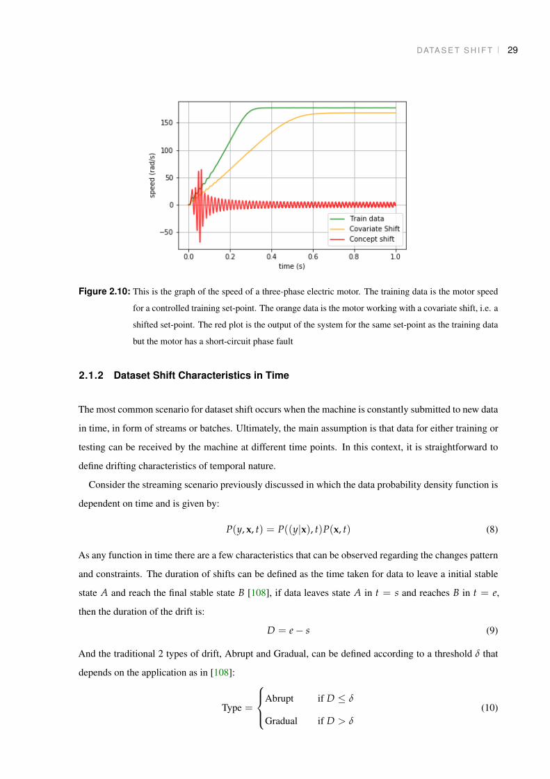
Another example would be the training of a system with specific operational set-points, but during
application the behaviour of the system is different. Thus, covariate shift occurs if set-points differ from
expected and, in case of some fault, concept shifts are as in 2.10.
DATA S E T S H I F T 29
Figure 2.10: This is the graph of the speed of a three-phase electric motor. The training data is the motor speed
for a controlled training set-point. The orange data is the motor working with a covariate shift, i.e. a
shifted set-point. The red plot is the output of the system for the same set-point as the training data
but the motor has a short-circuit phase fault
2.1.2 Dataset Shift Characteristics in Time
The most common scenario for dataset shift occurs when the machine is constantly submitted to new data
in time, in form of streams or batches. Ultimately, the main assumption is that data for either training or
testing can be received by the machine at different time points. In this context, it is straightforward to
define drifting characteristics of temporal nature.
Consider the streaming scenario previously discussed in which the data probability density function is
dependent on time and is given by:
P(y, x, t) = P((y|x), t)P(x, t) (8)
As any function in time there are a few characteristics that can be observed regarding the changes pattern
and constraints. The duration of shifts can be defined as the time taken for data to leave a initial stable
state A and reach the final stable state B [108], if data leaves state A in t = s and reaches B in t = e,
then the duration of the drift is:
D = e− s (9)
And the traditional 2 types of drift, Abrupt and Gradual, can be defined according to a threshold δ that
depends on the application as in [108]:
Type =
Abrupt if D ≤ δ
Gradual if D > δ
(10)

DATA S E T S H I F T 30
Patterns of Change in Time
time
P(x,y)
(a) Abrupt
time
P(x,y)
(b) Gradual
time
P(x,y)
(c) Incremental
time
P(x,y)
(d) Reocurring
time
P(x,y)
(e) Periodic
time
P(x,y)
(f) Outlier (not shift)
Figure 2.11: Graphical representation different dataset shift behaviours in time [36].
The first thing that need to be observed in any changing data is its speed, i.e. whether it is a tendency
or a step [25, 118]. Overall, there are two principal patterns of shift regarding its speed:
A B R U P T An abrupt shift occurs when there is a sudden change in the data behaviour, such as the
fault of a sensor in the plant. In this case, the probability distribution of the data P(y, x, t) is very different
from P(y, x, t + 1). In linear systems theory, this would be equivalent to a step disturbance.
A straightforward shift that occurs abruptly is the implementation of a system trained with a similar
case or a simulation. This is often the case of Mobile Ad-hoc Networks (MANETs) [37], but might
appear other system identification and control problems. A example of this issue would be a learning
machine of an audio system, which was trained with data collected indoors but the testing and application
was outdoors with different equipment, as seen in Fig.2.12.
Figure 2.12: Example of audio data collected indoors(red) and outdoors(blue), where street noise had a expres-
sive impact on the overall data. A machine trained for with the indoor data should compensate
possible background noise.

DATA S E T S H I F T 31
G R A D UA L Gradual changes are subtle and can be perceived as a trend in data, in real-world sce-
narios this would be observed in sensors ageing or thermal effects. Often, gradual shifts comprise of
a change between two concepts that is not concluded in a single transition. Consider the case where a
concept drifts from A towards B with an oscillation between these two states, which causes the concept
to change from A to B and back to A. The shift is said to be gradual if it progressively stays less time
in A and more in B, remaining there at the end of change. Gradual changes are regularly too subtle
to be noticed in subsequent moments and P(y, x, t) might appear to be similar to P(y, x, t + 1), how-
ever the shift trend is present and becomes visible in a larger time spam or with a smaller threshold for
changes. However the observation of gradual shifts require balance, since increasing the observed time
spam might cause the system to perceive the changes too slowly, and a smaller threshold might make it
too sensible to noise. The equivalent signal for an gradual shift, in linear systems theory, is the ramp.
A practical problem would be the identification of people in pictures from multiple stages of their
lives, as in Fig. 2.13, but with a limited set labeled pictures. This could be applied to face identification
in social media pictures or even in missing children cases [78, 91].
Figure 2.13: Incremental Shift represented by pictures of a person in her infancy (Initial State A), child-
hood, teenage and adulthood (Final State B), The L2 distance to the A state was calculated with
OpenFace[4].
Otherwise, if data is generated by different sources, this might cause targets to differ for the same
covariate, depending on the source that generated the data. Thus, shifts could occur with data collected
at the exact same time. Take, for instance, a market research problem, in this case, consumer patterns
change depending on their living area or niches, [8], thus shifts occur geographically when using a model
trained for a specific market across the others. Another example is the TeleECG of Federal University of
Minas Gerais [72], which is part of a semi-automatic health program. In this system, electrocardiograms
exams are made in hundreds of remote locations and diagnostics evaluation is centralized with automatic
triage. Since several exams are made simultaneously and exams conditions may change, due to nurse
technicians’ ability or equipment condition etc., then shifts appear both in time and geographically.

DATA S E T S H I F T 32
The trend of the change is precisely the information about the shift that needs to be incorporated to
the machine learning model in order the improve its performance. Thus, other complementary pattern
interpretations can be derived from these two main patterns to better explain the shifts behaviour [118]:
I N C R E M E N TA L Incremental drift occurs when sudden changes causes a trend in data. It can be
seen as a “staircase”, where each step is an abrupt change, but overall there is a gradual shift trend.
R E O C C U R R I N G The shift recurrence defines whether the change shifts towards a novel concept or
if it returns to previously visited, or reoccurring, ones.
P E R I O D I C Periodic shifts can be understood as reoccurring shift in which the concepts are revisited
according to a temporal pattern:
P(y, x, t) = P(y, x, t + nT) ∀n (11)
where T is a constant period.
O U T L I E R An outlier, otherwise, is a type of change in where a novel concept is visited without,
however, sustaining that state, nor indicating any trend or recurrence characteristics. Since an actual
statistical reflex does not exist, outliers are not considered dataset shifts.
Time Constraints of Shifts
The time constraints of the drift define whether it is:
P E R M A N E N T A dataset shift is permanent if effects of the drift remain over the data distribution
for an unlimited amount of time.
T R A N S I E N T In this case the effects of the dataset shift vanishes after a particular amount of time.
2.1.3 Causes of Dataset Shift
Through the stand point of the implementation of algorithms which target dataset shifting problems, the
first step is to define the causes of the drift. Overall machine learning methods should ideally be robust
to the data generators and retrieve any knowledge from the data itself. However, it is often common
pre processing data to deliver more significant or better conditioned information or features, for instance

DATA S E T S H I F T 33
through feature selection methods. These strategies do tend to improve models in machine learning and
should be smartly applied, so understanding the phenomena which causes any type of change in data is
the very first step to solve dataset shifting problems.
Knowing what type of dataset shift is present in data, or even if any type occurs at all, can be a very
challenging. However there are several situations that typically leads to one or more types of shift. In
this section we will briefly discuss some of them in order to facilitate the analysis of popular current
approaches for dataset shifting.
Sample Selection Bias
A common cause of Dataset Shift is related to the selection of a uniform, or biased, sample for training.
In this case, the training set choice is often obtained according to the conditional probability in Equation
12, with influence of a sampling decision variable s. Meanwhile, the test set is not subject to this decision
variable and is defined by the probability in Equation 13 [77, 67]. Specifically, the training data selection
is not performed randomly, and, instead, characteristics from the data targets y and covariates x are used
to decide whether the data should be used or not.
Ptrain(s = 1|x, y) (12)
Ptest(y, x) (13)
Where the sample are selected when s = 1 and discarded when s = 0.
The choice of an adequate data sample in fact require some knowledge of the system targets and
covariates, because simple covariate shifts and prior probability shifts might occur when the training
data do not properly define the input space. For instance, Dataset Shift ensues when part of the system
domain where the test covariates, lighter dots displayed in Figure 2.14, would most likely be is actually
excluded by the arbitrary selection function defined by s, hence resulting in a misspecified model caused
by covariate shift. Another shift scenario is the ” regression to the mean “, that occurs when the choice
of the sample is based upon the targets but is done naively.
The Sample Selection Bias problem might occur in three distinct manners: Ptrain(s = 1|x), Ptrain(s =
1|y) e Ptrain(s = 1|x, y) [67]. A sampling system is denominated MAR (Missing at Random) occurs
when the sample selection depends on x, i.e. Ptrain(s = 1|x), which characterizes covariate shift. Simi-
larly, prior probability shift occurs when the sample choice is related to y, causing Ptrain(s = 1|y). The
lack independence regarding both to x and y is a sampling system denominated MNAR (Missing not at
Random), which might lead to any type of Dataset Shift, or even to several of them[77, 67].

DATA S E T S H I F T 34
y
x
s
Figure 2.14: The selection variable s and its selection function given by the equiprobable contour define which
data are sampled [77]. Where darker dots are the training set, the lighter ones are the test set and the
contour is the boundary of the selection function.
The issue of bias in estimators may be induced by unequal selection probabilities at any stage of
sampling. This problem was addressed by [75], where consistent estimators were obtained by weighting
the model estimation using the reciprocals of the selection probabilities at each sampling stage.
Imbalanced Datasets
A common problem in data classification, specially in multi-class cases, is the quantity of data patterns
presented by each class, named data balance. Unbalanced datasets are defined when one or more classes
present much fewer data then the others. However, this is problematic since the correct classification of
smaller classes becomes significantly harder when their rarity of increases [32, 58, 59]. Differences in
balance between testing and training sets in classification problems are a prior probability shift scenario,
thus imbalanced datasets can use methods aimed to prior probability shifts to mitigate the problem [2, 43].
However, in Dataset Shift context, another important issue arises when attempts of class balancing are
made, since they tend to induce a sample selection bias with known bias. The dataset shift occurs when,
in order to rebalance data, patterns of the more populous class are discarded in a manner that the training
data distribution becomes different from the test set distribution [77].
In order to minimizes possible Dataset Shifts, the authors in [59] balance the classes through partition
of the dataset using “Distribution optimally balanced stratified cross-validation”. The same authors, in
[58], solves the problem of unbalanced classes using different intrinsic characteristics of the data. The
hepatitis dataset [21] was used as an example of this issue in Fig.2.16.
Model generation and selection is hindered when the training data is heavily unbalanced since most
modelling process tends to favour the dominant class. Ideally both classes should have a comparable
amount of data, thus a common practice is to exclude patterns from the most populous class. This
strategy is often used since it is usually extremely costly to obtain enough rare cases to equalize both
classes [32, 58, 59, 98]. For instance, in the two class classification problem in Figure 2.15, the training
set, represented by the lighter dots, has been under sampled in order to rebalance the classes, represented
by the circular contours, however in the test data, in darker shade, the imbalance still exists.

DATA S E T S H I F T 35
y=0
y=1
x1
x2
(a) Imbalanced datasets with a classification
model(solid lines).
y=0
y=1
x1
x2
(b) Under sampling conditional model to rebal-
ance data, causisng missepecified models
(dashed lines).
Figure 2.15: Dataset shift caused by class rebalance for a two class case example, where the darker dots are
training data and lighter ones are test data [77].
(a) Original Imbalanced datasets with a Gaussian SVM
classifier, with 85% cccuray for the test set (dots black
border).
(b) Under sampled rebalanced data with a Gaussian SVM
classifier, with 63% accuray for the test set.
Figure 2.16: Projection of the features Albumin and Prothrombin Time from the Hepatitis dataset. Class Live
(green) has significantly more instances than class Die (red in Fig 2.15a. The under sampling pro-
cess dependent on values of other features, such as Malaise, Age and Histology, resulted in the
misspecified models in 2.15b, with the class contours significantly different.

DATA S E T S H I F T 36
The work in [107] is a systematic study regarding imbalanced classes and dataset drift. In it, there are
compelling comparison and analysis of state-of-art methods when applied to class imbalance problems
with concept drift in one-by-one on-line learning. This paper verifies six different methods to handle
either data imbalance, drift or both.
Non-Stationary Environments
Real problems are, in general, never completely stationary in time and space. In addition, the environ-
ment is not usually completely controlled or modelled, which causes data extracted from the system to
present variations between training and testing. Sometimes these changes are known and can be ob-
served, however adjusting the model at every moment, even for a known shift, can be very costly. In
other scenarios, changes can be unexpected, unobservable or even unknown which forbids tuning the
model at any point [67]. In both cases learning strategies that intrinsically consider these changes in data
are appropriate solutions.
Learning in non-stationary environments is greatly related to streaming and on-line problems, but
not exclusively. The data generating process of non stationary environments is often characterized by
evolving phenomenon. In this subject, [25] is a comprehensive survey on non-stationary environments
that should be addressed for further information on the topic.
Domain Shift
Domain Shift, in particular, occurs when the measurement system, the metrics or even the description
of the data generator changes. This shift is illustrated by the currency devaluation in a prices prediction
system, or the visual classification of images with lighting changes.
A domain is considered when the input covariate x is not directly the latent variable, named here x0,
but is, instead, an observation of this latent variable by a function, x = f (x0). When the function f (x0)
suffer some change the covariate x perceived by the model is different even if the latent variable x0
remains the same. Then, a difference between the training and testing domains could take place even
if the latent variable x0 and its relation to y remains constant, because the targets distribution P(y|x0)
depends on the latent variable x0 while the model selection input depends on a function x = f (x0).
For instance, in the image classification example, the model inputs are not the scenes themselves, they
are, instead, photographies taken with very specific settings. In this case, the photographies are outputs
of an observation function and a shift in this function could be represented by different lighting settings.
Thus, the photographies, or covariate x, taken with poorer illumination are very different from the ones
taken in a brighter environment, even if the scene remains the same.
DATA S E T S H I F T 37
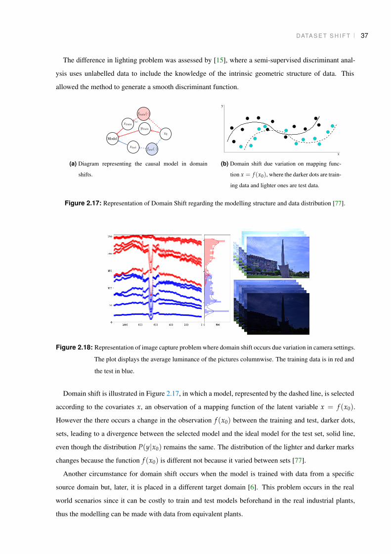
The difference in lighting problem was assessed by [15], where a semi-supervised discriminant anal-
ysis uses unlabelled data to include the knowledge of the intrinsic geometric structure of data. This
allowed the method to generate a smooth discriminant function.
xtrain
ftrain(·)
x0
ytrain
f (x0)
Model
ftest(·)xtest
(a) Diagram representing the causal model in domain
shifts.
y
x
(b) Domain shift due variation on mapping func-
tion x = f (x0), where the darker dots are train-
ing data and lighter ones are test data.
Figure 2.17: Representation of Domain Shift regarding the modelling structure and data distribution [77].
Figure 2.18: Representation of image capture problem where domain shift occurs due variation in camera settings.
The plot displays the average luminance of the pictures columnwise. The training data is in red and
the test in blue.
Domain shift is illustrated in Figure 2.17, in which a model, represented by the dashed line, is selected
according to the covariates x, an observation of a mapping function of the latent variable x = f (x0).
However the there occurs a change in the observation f (x0) between the training and test, darker dots,
sets, leading to a divergence between the selected model and the ideal model for the test set, solid line,
even though the distribution P(y|x0) remains the same. The distribution of the lighter and darker marks
changes because the function f (x0) is different not because it varied between sets [77].
Another circumstance for domain shift occurs when the model is trained with data from a specific
source domain but, later, it is placed in a different target domain [6]. This problem occurs in the real
world scenarios since it can be costly to train and test models beforehand in the real industrial plants,
thus the modelling can be made with data from equivalent plants.

DATA S E T S H I F T 38
Source Component Shift
The source of any real-world data is subject to variations, moreover data is often generated from multiple
different sources, and each of them is prone to disturbances. In this case, the overall distribution of the
covariates can easily differ between training and testing, thus a correct model selection becomes difficult.
M I X T U R E C O M P O N E N T S H I F T When a problem data is generated by a certain number of sources,
each one is responsible for different amount of data, it is possible that the proportions of data from each
source change amid the test and the training sets. Given that the source for each data is, in fact, unknown
this problem might be featured as prior probability shift[77].
F AC TO R C O M P O N E N T S H I F T In a problem in which the probability of the data is influenced by
factors that might be decomposed in form and strength, if the form of the factor remains constant but its
strength changes from the training to the test sets, it is characterized the Factor Component Shift[77].
M I X I N G C O M P O N E N T S H I F T In this case, there are several similarities with the Mixture Compo-
nent Shift, since both relate to the same context. However, in the Mixing Component Shift the data are ag-
gregated so that it is observed an average of x of a population which could present a great variability[77].
The EEG problem in Fig.2.4 is a typical example of Source component shift. Since brain activity is
extremely complex and noisy, several electrodes need to be used and the data dimensionality is usually
through filters and feature extraction methods [69], which causes shift due to data aggregation. Shift also
occurs in EEG itself since each electrode measures an average stimuli in a brain region. Because of it,
small deviations in electrodes placement aggravate dataset shifts.
2.1.4 Learning Strategies for Shifting Datasets
Nearly all learning strategies for dataset shift are based in two approaches, named active and passive.
Essentially, active approaches detect shifts and adapt the model learning according to changes in data,
meanwhile passive approaches are overall robust to shifts that may occur to the data[25].
However, in machine learning, there are numerous other possibilities to solve Dataset Shift problems.
For instance, the methodology in [93] performs the mining of rules the governs dataset shifts. There, the
authors draw these rules with the aid of a mining tree, named Concept Drift Rule mining Tree (CDR-
Tree). In this case, classification models are created directly by the extraction of the drift rules for each
data configuration.

DATA S E T S H I F T 39
Active Approach
Adaptive learning models have the prerogative of updating their parameters whenever a change in data
is detected. With this approach, the model can be optimized for the data it receives at any given moment.
For this, two important structures must exist in the leaning process: a Change Detector and a Adaptation
Mechanism[25], as seen in Figure 2.19.
Classifier
Model
Adaptation
Shift
Detection
Input
Output
Update
Shift Detected
Active Learning Diagram
−
Figure 2.19: Active approaches use a change detector to inspect the inputs and/or classification error over the
labelled samples. The detector signs the adaptation mechanism to update the classifier[25].
S H I F T D E T E C T I O N Shift detectors are one of the main components of active approaches. It ob-
serves the data and, through tests or other comparison methodologies, indicates if a change in data has
happened. Among numerous shift detection methods, statistical hypothesis testing on the multivariate
data is a straightforward well established method. However, most of these statistics tests depends on
a fixed set of characteristics from the underlying distribution. If the drift causes small changes on the
properties observable by the statistics methods, the detector tends to perform poorly[27].
Three adaptive detection methods were proposed by [27], in which the first one uses a rank statistic
based on the density estimates of a binary data representation. The other two uses support vector ma-
chines (SVM) in their implementation, one compares the average margins of linear classifiers induced
by 1-norm SVM, and the last one examines the average zero-one, sigmoid or stepwise linear error rate
of SVM classifiers.
The authors of [81, 82] introduce a series of methods employing an exponentially weighted moving
average (EWMA) for the detection of some Dataset Shift problems, in particular the covariate shift. For
electroencephalogram(EEG) based Brain-Computer Interfaces(BCIs), [83, 80] used the covariate shift
detection based on an exponential weighted moving average to identify drifts in the principal component
analysis of features extracted from motor imagery-based brain electrical responses.

DATA S E T S H I F T 40
A simple detection system was proposed in [35], where the error of the learning system is monitored
in two stages. If it surpasses a warning threshold, the system verifies if the error increases until reaching
a drift threshold. When the drift is then detected the learning system is retrained according to the samples
received between the warning and the drift points.
A semi-supervised approach that monitors efficiently changes in the classifier confidence to detect
shift was proposed by [41]. This approach exploits dynamic programming and selective executions of
the detection module in order to make the method feasible.
Dynamic systems modelling are used in [17] to create detection mechanisms for high frequency data
streaming. It is argued that supervised and semi-supervised strategies are infeasible for such scenarios,
thus the authors propose unsupervised methods based on dynamic models. This paper proposes four
different strategies using phase spaces, among them is their comparison using the Gromov-Hausdorff
distance, and the application of Cross Recurrence Plot and Recurrence Quantification Analysis to detect
drift in consecutive phases.
Passive Approach
Another possibility to solve problems with Dataset Shift is modelling with an underlying assumption that
data will change, thus the model itself adapts for every new data it receives despite of actually occurring
a drift or not. These methods tend to be specially robust on gradual or incremental shifting scenarios.
An early approach was proposed in [44], where the intrinsic mode functions of the model are adaptive.
The method is based in the empirical decomposition of the data, allowing a well-behaved Hilbert trans-
form for each function. Since this decomposition concerns local characteristic time scales of the data, at
singular time instants the method can be considered a passive adaptive approach.
The method proposed in [47] modifies da data window used in order to minimize the estimated gener-
alization error. Though this method can be used to somewhat detect drifts according to the window size,
it is actually a passive approach since the windows sizes are adjusted with every batch input given to the
system. Furthermore, this method is similar to cross-validation, where several models with all possible
widows sizes are trained, then the window size with the lower estimated error is chosen.
Through a simple analysis of the problem, the parameters of multinomial random variables can be
estimated with regard to the first and second moments according to principles of stochastic learning, as
done in [70]. Though this paper explanation of the method application in machine learning be quite brief,
it is presented examples with pattern recognition problems.
Another possible passive approach is the preprocessing of data, making it possible for traditional
learning algorithms to track drifting data. This framework is proposed by [110], where a computational

DATA S E T S H I F T 41
framework for extending incomplete labelled data stream (FEILDS) transforms the original data stream
with a few labelled data into a new one that incorporates the concept drift.
2.1.5 Popular Approaches for Dataset Shifting Problems
Transductive and Semi-Supervised Learning
Transductive and semi-supervised approaches use unlabelled data in combination with labelled datasets
to improve classification. These methods are interesting to solve a variety of shifts, since they are capable
of using the test data to incorporate more knowledge into the model and, thus, retrieve information that
might have changed between the training and test sets.
Transduction classifies and perform regression of data without an induced general model, by consid-
ering both training and test data to compute every output. Therefore this method is able to intrinsically
handle several types of divergences without requiring an active mechanism to detect or track any types
of drifts. Moreover, the overall test error of this method is not affected by differences between training
and test sets since the joint error 3 is related particularly to induced models. Thus, transductive learn-
ing strategies are very intuitive for passive approaches, since they are robust to dataset changes without
reacting to detected shifts.
Approaches that incorporate Support Vector Machines (SVM) with transductive and semi-supervised
strategies, such as Transductive Support Vector Machine (TSVM), have been greatly studied in the liter-
ature [7]. The TSVM method, despite of incorporating large margin classification and information from
unlabelled data, might present lower performance then the traditional SVM if not well tuned[104]. An
application for TSVM was proposed by[12], where a specific procedure for binary transductive SVM
was proposed for remote-sensing classification with ill-posed data and small-sample sizes.
In this context [24] proposed an ensemble algorithm with transductive learning, named TRANSE, in
order to solve the drift problem by assuming that the test data is sample i.i.d. of an unknown distribution.
However, since transductive learning might be very costly, active approaches can also be implemented.
In [83, 80], a system is updated according to a transductive learning strategy whenever the covariate
shift detector signs a drift. The learning approach is based on a probabilistic K-nearest neighbour (KNN)
method and defines a knowledge base according to euclidean distance between the labelled and unla-
belled data points. This base obtained through the transductive approach at each covariate detection
is combined with the existing knowledge base. Then, the inductive classifier function of the model is
adapted according to the final knowledge base.
Semi-supervised approaches, in a broad sense, consists of usually inductive modelling strategies that
use both labelled and unlabelled data during training. In [15], a semi-supervised discriminant analysis

DATA S E T S H I F T 42
was proposed from a Linear Discriminant Analysis (LDA) stand point. In this approach, the classifier
is obtained by maximizing the inter-class covariance and minimizing the intra-class. Consider that, for
small training sample sizes, the covariance matrix of each class may not be accurately estimated. Thus
a semi-supervised approach was proposed in order to include the knowledge from unlabelled data of the
intrinsic geometric structure of data.
An application subject to concept changes is voice recording studied in [111], where it was modelled
as covariate shift. In this paper, it is proposed a semi-supervised method that comprises of weighted
versions of kernel logistic regression and cross validation approach.
In real-world scenarios, the drift in sensors are present in several types of applications, specially caused
by sensor ageing or cumulative residuals. Drifts in artificial olfaction were investigated by [18], where
semi-supervised methods were applied to long-term on-field continuous operation of chemical multisen-
sory devices with drift-induced performance degradation.
Incremental and On-line Learning
In a scenario where data is constantly changing, an incremental learning approach, in which the model is
continuously updated in order to expand the model knowledge, holds great value since, by definition, it
is adaptable to data changes [54, 25]. Incremental learning approaches can be passive, as it may consist
of dynamic techniques that incorporate new knowledge to the model as data becomes available despite
of it being shifted or not.
However, some solutions for concept drift were studied in [109], under an aspect of on-line incremen-
tal learning. It was proposed that trusted contexts are memorized so that they can be used when they
appear again. This paper applies a heuristic to constantly monitors the behaviour of the system, which
characterizes an active approach to a concept drift.
The Learn ++.NSE is an incremental learning algorithm which works with batches of data. For
every new batch, it creates a new classifier that is integrated to an ensemble of classifiers according to
an age-adjusted dynamic error based weighted majority voting [29, 22, 30]. The Learn ++.NSE has
showed to be able to track changing environments and is capable of accepting additions and subtractions
of classes. Also, further studies have shown that this method is robust to class imbalance when combined
with Synthetic Minority Over-sampling Technique (SMOTE).
An Extreme Learning Machine was proposed in [57]. Named Forgetting Parameters Extreme Learning
Machine (FP-ELM), it defines a mechanism of on-line learning that decreases the importance of older
chunks or batches of data as new ones arrive. In this method the weight attributed to older chunks is
shrunk by a forgetting parameter in order to guarantee the method performance for the most recent data

DATA S E T S H I F T 43
context. This method has shown to perform comparably and to be equivalent to more complex and costly
ensemble methods.
[87], proposes a kernel ensemble learning method that updates the system whenever the true labels are
available. This method redefines the boundaries of the classes in the feature space whenever it receives
new labelled data.
An active incremental learning strategy was proposed by [85], where a window-based technique esti-
mates the score of concept drift for each unknown email. The model, then, continuously incorporates
new spam keywords and updates the filtering decision process.
Specifically for regression problems, in 2015 a second order on-line method was proposed in [68].
Regression models tend to have more consolidate approaches based on adaptive filtering and control
methods, thence this paper regards particularly an on-line machine learning by incorporating two adap-
tive approaches: (i) an adaptive covariance reset to forget older contexts, and (ii) a last-step min-max
optimization of the predictor.
The on-line learning approach was systematically studio regarding the problem of class imbalance
with dataset shift by [107]. In this paper the techniques presented in [105], [106], [13], [103], [65] and
[39, 71].
Transfer Learning and Domain Adaptation
There is a great relation between the Dataset shift and the transfer learning, given that this type of
learning considers that the training can be performed with barely a limited amount the possible settings
of the training data, in such a manner that the prediction for specific settings is improved. Hence the
survey in [73] might be an interesting view of the matter.
Strictly the approach proposed by [110], is a possible framework for transfer learning, as it attempts
to learn and encode invariances from a limited set of labelled data prior the learning stage.
In a similar context, Domain adaptation consists in the adjustment of a given classifier created in an
initial context, source domain, into a new one, target domain, without the necessity of data from the
new context or using a very reduced amount. The papers [51], [62] and [114] have proposals with such
approach.
The strategy proposed in [46], exploits bias in data during training as it accounts for biased vectors
weights, associated with individuals datasets, and visual world weights, common to all datasets. The
visual world weights are retrieved by withdrawing the bias weights from each dataset, which allows a
model training with an essentially unbiased datasets.
Another approach to domain adaptation was proposed in [66]. In this paper the performance of an
existing classifier was improved with the feature extraction of a new dataset with a genetic based algo-

DATA S E T S H I F T 44
rithm. In this case a classifier for biological laboratory data for cancer diagnostics was improved with
the incorporation of data from a different laboratory that uses the same protocols.
Ensemble Learning
Model misspecification often occur because the data has different behaviours throughout the input do-
main, leading to drift when de data used for testing is limited to particular domain regions. A possible
and effective approach, as seen in Fig. 2.3b, is to define multiple local models throughout different re-
gions the input domain. In machine learning, this strategy can be achieved through ensemble learning
methods [54, 76].
Ensemble learning techniques are often intrinsically capable of defining the current data context. Usu-
ally, each model within the ensemble committee is related to a given context, which allows this method to
define the current context and the best model for such context. However, for this approach, the contexts
should be know a priori. In [94], for instance, a dynamic integration of classifiers is performed so that
the local accuracy of each classifier with regard to the instance tested is used to select the best classifier
or set of weighted classifiers.
The characteristics of diversity on ensemble learners has been studied in [63, 64], there it was ob-
served that, though more diverse ensembles present lower test errors shortly after the drift, afterwards
the diversity becomes less important and do not allow faster recovery in long-term.
In [48], some methods are implemented to trace context shifts using on-line learning and dynamic
weighted majority to define an ensemble of learners. This papers results showed an overall high accuracy,
also the ensemble method have shown to be capable of learning drifting contexts with almost the same
accuracy as the base algorithms learn each concept individually. In [49], the same authors proposed an
additive expert ensemble algorithm, named AddExp, which is a method that can be applied to any on-line
learner for drifting contexts.
A semi-supervised approach was used, in [23], for solving non-stationary environments, it updates
the weights of an ensemble classifier using unlabelled data unknown distributions. In [24], an ensemble
approach was used integrated with transductive learning.
The Learn ++.NSE [29, 22, 30], which was previously addressed, is an incremental learning algo-
rithm that generates dynamic ensembles according to the data batches that become available.
More recently, in 2015, a method to create an ensemble of subset on-line sequential extreme learn-
ing machine (ESOS-ELM) was proposed by [65]. This framework consists of an active approach as it
includes a change detection mechanism, ir comprises as well a short-term memory system in its main
ensemble and a long-term memory structure in an information storage module.

DATA S E T S H I F T 45
An ensemble method based on the Random Forest Algorithm was proposed by [116]. A Accuracy
Weighted Ensemble (AWE) method was implemented in which the majority voting weights use base
learners accuracy and intrinsic proximity measure of Random Forest.
Kernel ensembles were also applied to evolving concepts in data stream in [87]. The authors propose
a multiple kernel learning approach where the boundaries of classes in the feature space of combined
kernels are specified in order to reduce memory usage. And the evolving of the kernels is performed
whenever new labelled data is available, by changing to the class boundaries previously defined.
Active Learning
Regarding predictive models, the active learning approach attempts to select the minimum possible
amount of labelled data required to develop an accurate model. As to dataset drifting, the predictive
models need to adapt to changes in data, which is addressed in [117]. In this paper, a framework for ac-
tive learning that explicitly handle concept shifts was proposed. For this, dynamic allocation of labelling
and randomization of the search space are performed.
The active learning applied to solve the covariate shift in Dataset Shift is approached in [96, 95]. This
paper explores remote sensing image classification, in which shift occur simultaneously for two different
reasons Sample Selection Bias and Domain Shift. In this scenario, the image is classified accord to
sampled pixels in the image, which addresses the first cause for shifting. In order to improve this issue,
the author attempt to select the pixels in an intelligent manner. The domain shift is characterized in
changes in illumination or geometry which hinder transfer classification models. Therefore an active
approach was proposed to adapt the models to similar images, herein the known distribution is adapted
according to model uncertainties criteria and the unknown classes are included according to a clustering
criteria. The active sampling was decisive to permit a fast convergence and an optimal adaptation.
Weighted Approaches for Covariate Shift
Several methods attempt to solve dataset shift related problems by weighting data intrinsic characteristics,
such as the inputs, the probability densities, [86] proposes a method that deals with the covariate shift
using a function log-similarity with weighed input samples, thus this method is adequate in situation in
which the pdf of the observed samples do not correspond to the total population.
For binary classification, [88] solve the bias in cross validation caused by covariate shift through an
importance weighted cross validation method, where the ratio between both classes is used to remove
almost completely the bias in cross validation risk. The importance is also addressed in [89], where
direct importances are estimated without any probability density estimation.

S TAT I S T I C A L D I S T R I B U T I O N S C O M PA R I S O N 46
The detection of covariate shift through exponentially weighted moving average (EWMA) was vastly
studied by [81, 83, 82, 80]. This method uses statistical process control charts to detect shifts in the input
covariate.
2.2 S TAT I S T I C A L D I S T R I B U T I O N S C O M PA R I S O N
In order to asses a divergence between two populations, e.g. training and testing datasets, it is necessary
to choose the appropriate measure to compare them. The selection of suitable measurement coefficients
depend on the objectives of the comparison, which should be rather precisely stated. For the purpose of
clustering, and thus partially the drifting issue, a large class of measures may lead to similar conclusions.
Therefore, the consistence of the final conclusions could be verified using a set of two or more possible
measures [79]
2.2.1 Dissimilarities and Similarities Measures
Another approach for comparing two different distributions is defining how similar they are, instead of
measuring their difference. In this case, there are similarities coefficients
Kullback-Leibler Divergence
The Kullback-Leibler Divergence is a metric based in Entropy, thus also being named relative entropy,
proposed by [53]. The paper ”On Information and Sufficiency“ the authors investigate the measure-
ment of the distance or, more accurately, divergence between statistical populations with the use of the
Kullback-Leibler divergence to retrieve information, for statistical discrimination problems.
The equation 14 is the definition of the divergence for continuous random variables Xi and Xj. Where
probabilities pi(x) pj(x) exist, if there are available observations of the probability functions Pi and Pj
over the set X comprised of Xi and Xj observations. KL divergence, then, is defined as equation 15, in
which dP/dQ is the Radon–Nikodym derivative.
DKL(
Pi‖Pj)=∫ ∞
−∞pi(x) log
pi(x)pj(x)
dx (14)
DKL(
Pi‖Pj)=∫
Xlog
dPi
dPjdPi (15)
The equation 16 is the KL divergence for discrete probability distributions Pi(k) Pj(k):
DKL(
Pi‖Pj)= ∑
kPi(k) log
Pi(k)Pj(k)
(16)

S TAT I S T I C A L D I S T R I B U T I O N S C O M PA R I S O N 47
Observing equation 14, it is possible to notice that the Kullback-Leibler divergence is not symmetric,
nor is bounded to always be finite. Hence, the relative entropy is not reflexive, not being considered, then,
a distance metric. However, it does measure the difference between the informations in two different
distributions.
The Kullback-Leibler divergence is not restricted to parametric formulations of probability distribu-
tions, however, it is convenient to define the divergence for the comparison of two Normal distributions
with dimension n:
DKL(Ni‖Nj
)=
12
(tr(
Σ−1j Σi
)+(µj − µi
)> Σ−1j (µj − µi)− n + ln
(det Σj
det Σi
)). (17)
In statistical inference, the minimization of the Kullback-Leibler divergence between a observed coor-
dinate to a specific point is the maximum likelihood estimator at that point [3]
Fisher Information Metric
The Fisher Information Metric is a smooth statistical manifold, more specifically, it is a particular case
of the Riemannian metric. In practice it allows the calculation of the information difference between two
measurements, since its points are probability measures defined on a common probability space. This
measure is represented in matrix form, thus being, firstly, known as Fisher Information matrix.
Given a random variable X with observations x, with probability normalized according to:∫X
p(x, θ)dx = 1 (18)
Let Θ = (θ1, θ2, θ3, . . . , θn) be the coordinates of a Riemannian space, that forms a smooth manifold
which the metric tensor gij is defined by the Fisher information matrix [3]. Then, on order to retrieve the
dissimilarity information between two coordinates, the Fisher metric takes the following form:
gij =∫
x
∂ log p (x, θ)
∂θi
∂ log p (x, θ)
∂θjp (x, θ) dx (19)
It can be observed that, in a metric context, the Fisher Information metric is the second derivative
of the relative entropy, therefore it is the Hessian of the Kullback–Leibler divergence. Thus, the Fisher
information is a symmetric positive, semi definite matrix. In this context, for discrimination between
distributions, the θ are considered parameters of the probability distributions fisher equation could be
written as:
gij =∫
x
∂ log pi (x)∂θi
∂ log pj (x)∂θj
p (x, θ) dx (20)

S TAT I S T I C A L D I S T R I B U T I O N S C O M PA R I S O N 48
Jensen Shannon Divergence
Kullback-Leibler Divergency, however, is not symmetric, which might cause it not to be adequate in
several applications, including in distance measure. In this context, the Jensen-Shannon Divergence is a
symmetrized and smoothed version of DKL [56, 33], where:
DJS(
Pi‖Pj)=
12
DKL (Pi‖M) +12
DKL(
Pj‖M)
(21)
with
M =12(
Pi + Pj)
(22)
In the scope of mixture models or joint distributions, the Jensen-Shannon Divergence could be gener-
alized as:
DJS(
Pi‖Pj)= H
(πiPi + πjPj
)− πi H (Pi)− πjH
(Pj)
(23)
with weights πi, πj ≥ 0 and πi + πj = 1, and H is the Shannon Entropy, which is defined for a discrete
random variable X, with probability mass function p(x) as:
H (X) = E [− log (p(X))] (24)
And the conditional entropy between two random variables Xi and Xj is:
H(Xi|Xj) = −∑k
∑m
p(xik, xjm) logp(xik, xjm)
p(xjm)(25)
with p(xi, xj) being the probability of Xi = xi and Xj = xj.
In [56], is defined that the Jensen-Shannon Divergence is, then, bounded:
DJS(
Pi‖Pj)≤ H
(πi, πj
)≤ 1 (26)
Still in this context, the Jensen-Shannon Divergence is related to mutual information of discrete vari-
ables in defined in equation 27.Consider that the random variable X is composed by a mixture of distri-
butions Pi and Pj, with weights πi and πj. And a binary variable Z defines from which distribution each
realization of X is derived, choosing Pi when Z = 0 and Pj when Z = 1.
I ≡∑k
∑m
p(xik, xjm
)log2
p(xik, xjm)
πj p(xik)(27)
I(X; Z) = H(X)− H(X|Z)
=12 ∑ Pi (log Pi − log M) +
12 ∑ Pj
(log Pj − log M
)= DJS(Pi‖Pj)
(28)

T R A N S D U C T I V E L E A R N I N G 49
2.3 T R A N S D U C T I V E L E A R N I N G
In transductive settings, particular values of a functional dependence are directly estimated, without
necessarily having to estimate the general function itself. In this context, this estimation can be performed
by a number of different techniques, for instance, the approach for transductive learning proposed by [61]
uses statistical premisses. This thesis was the main reference for this work.
The general learning problem of model induction can be represented according to the functionality
of the four components of Figure 2.20. In the figure, there is a data generator (DG), which selects
random samples x ∈ χ ⊂ <n, drawn independently from an unknown but fixed probability distribution
function F(x). There is an oracle – or supervisor – (O), which returns an output value y ∈ Y for every
input sample x according to an unknown but fixed conditional distribution function F(y|x). There is an
evaluator (E) capable of implementing a set of functions f (x, α), α ∈ Λ, where Λ is an arbitrary set of
parameters that governs the behaviour of the function. Notice that by making Λ arbitrary, f (x, α) α ∈ Λ
may actually be any set of functions. Finally, there is a learning machine module (LM), that is capable to
select from the set of functions f (x, α) α ∈ Λ the one that best represents oracle’s response for a given
training set, which is a finite set of samples
(x1, y1), . . . , (x`, y`), (29)
drawn i.i.d. by DG and O with respect to the joint density F(x, y) = F(x)F(y|x).
Figure 2.20: Learning model based on inductive inference, where a function that best approximates the unknown
functional dependence is selected from the set of all possible functions based on the given training
data.
Once the machine is trained, the value α0 ∈ Λ is determined and produces the function f (x, α0)
through E that best approximates the unknown functional dependence. This approximation may then be
used by E to estimate unknown values y∗ at arbitrary points x∗ ∈ χ. This representation is similar to the

T R A N S D U C T I V E L E A R N I N G 50
classic one described in computational learning theory [45] . The difference between them is that here
LM and E are represented as different functional blocks.
Notice that, at anytime during training, LM may present any sample x ∈ χ to E and expect a response
y = f (x, α). For samples x in the set (29), y may be compared to the answer y provided by the oracle
O. This comparison is the basis of the selection mechanism that determines the approximation of the
functional dependence, and it is measured by a loss or discrepancy function L(y, f (x, α)) that yields the
estimation of the risk functional
R(α) =∫
L(y, f (x, α))dF(x, y), (30)
referred to as the expected risk.
The solution of the learning problem, implemented by LM, may hence be described as finding the
function f (x, α0) which minimizes the expected risk [100]. In other words, find the function f (x, α0)
that minimizes the risk functional R(α) over the class of functions f (x, α), α ∈ Λ, where F(x, y) is
unknown and the only data available is the training set (29).
The main issue here is whether or not the estimated risk yielded by the training set approximates the
expected risk as defined by Equation 30. Since only a restricted training set is available, the general risk
functional is then approximated by the empirical risk functional by making it discrete with respect to the
training set (29):
Remp(α) =1`
`
∑i=1
Q(zi, α), α ∈ Λ. (31)
where Q(zi, α) is a loss function calculated over the training samples.
Notice that Equation 31 does not depend on any knowledge about the joint densities, so Remp(α) is
fixed for a particular choice of α and for a particular training set (29) [14]. Assume that α0 and α1 are the
optimal parameter sets for the empirical functional risk and functional risk, respectively. We have that
Remp(α0) and Remp(α1) will converge to the same value as the number of samples N tends to infinity.
Despite being theoretically sound, the ERM principle is not well suited to deal with small data samples,
since convergence is achieved only when N is very large. This motivated the development of the so-
called Structural Risk Minimization (SRM) inductive principle [99]. The SRM principle, as the ERM
principle, also attempts to minimize the empirical risk. The SRM principle, though, simultaneously
attempts to minimize the confidence interval given by the bounds on the risk functional [100]. As a
result, the SRM principle is able to consider both the quality of the approximation of the data as well as
the complexity of the approximating function. Although an additional control of function approximation
can be made by SRM, it also depends on dataset size and representativeness. Since all the possible
functions f (x, α), α ∈ Λ can be searched for model selection, there is always an expectation that the
outcome with SRM will be close to the optimal solution.

T R A N S D U C T I V E L E A R N I N G 51
We now examine the transductive setting of the learning problem, on which one is not interested in
estimating the unknown functional dependence from a set of functions f (x, α), α ∈ Λ [115] [50]. Rather,
the goal is to estimate the values of this functional dependence at given points using a function f (x, α∗)
from the set f (x, α), α ∈ Λ. In order to accomplish the estimation for the specific points, one should be
able to use the information conveyed by these given points.
As with inductive inference, it is possible to obtain a learning model based on the same four compo-
nents for transductive inference (Figure 2.21). Three of these components, DG, O, E, are identical to the
inductive case. The difference relies on the learning machine LMT, which now not only takes as input
the original training set (29), but also a so-called working set DW
(x`+1, . . . , x`+k), (32)
also drawn i.i.d. by DG.
The working set represents the k points of interest where one wishes to estimate the values y∗ =
f (x∗, α∗) of the unknown functional dependence, where x∗ ∈ (x`+1, . . . , x`+k). Finally, the communica-
tion between DG and E becomes restricted, since E, despite being the same as in the inductive model, is
now only able to properly estimate values either on the training set (29) or on the working set (32). The
obtained model is not generic anymore. Notice that, as opposed to the inductive case, it is not necessary
for the unknown functional dependence to be a function of the set f (x, α), α ∈ Λ since now the search
is through a restricted set of functions aimed at the working set only.
Figure 2.21: Learning model based on transductive inference. A modified learning machine takes both training
and working sets as inputs, and the evaluator is only able to estimate values on either of these sets.
In the transductive inference setting, the solution to the learning problem, implemented by LMT,
may be described as finding the function which minimizes the overall risk. More formally, LMT must

G A B R I E L G R A P H S G AU S S I A N M I X T U R E M O D E L S 52
find the function f (x, α∗) that, with probability 1− η, minimizes the overall risk of estimating values
y∗ = f (x∗, α∗) for x∗ ∈ (x`+1, . . . , x`+k). This is analogous to minimizing the functional
RΣ(α) =1k
k
∑i=1
L(y`+i, f (x`+i, α)), (33)
where L(y, f (x, α)) is a generic loss function.
Notice how the measurement of risk differs from the inductive to the transductive settings of the
learning problem. In the inductive case, the risk functional (30) assesses the risk with respect to the
joint distribution function F(x, y) for the whole space of the unknown functional dependence. In the
transductive case, the risk functional (33) only assesses the risk with respect to the given points of interest,
i.e. the working set DW = (x`+1, . . . , x`+k). The analysis of Equations 30 and 33 helps to understand
how the risk is calculated in both inductive and transductive settings. Since DW ∈ χ, a tighter bound
for transductive learning risk could be expected. In fact, after Vapnik’s original work on error bounds
for TL [101], other authors have also pointed out to tighter bounds for TL risk [20, 5]. In practice, risk
bounds yield an estimate of the test error by minimizing the risk bound function, and are valuable to
choose an algorithm or a model. A tighter bound for TL may suggest, therefore, a better performance on
the working set.
Structural minimization of the overall risk is, in fact, the same as the inductive method of structural
risk minimization. The key difference lies in the availability, a priori, of the given points of interest where
one must estimate the values of the unknown functional dependence:
x1, . . . , x`, x`+1, . . . , x`+k. (34)
When estimating functions, one must determine the structure on a (possibly infinite) set of functions
f (z, α), α ∈ Λ given the set itself and the domain of definition of its members. When estimating values
at given points, a structure S1 ⊂ S2 ⊂ · · · ⊂ Sn on the set f (z, α), α ∈ Λ may be defined on the
equivalence classes of the set. A set is decomposed by a finite number of equivalence classes through
a set of indicator functions, where two indicator functions are said to be equivalent when they classify
elements of the complete sample given in (34) in the same way.
2.4 G A B R I E L G R A P H S G AU S S I A N M I X T U R E M O D E L S
Gabriel Graphs were proposed in[34] as an approach to analyze geographic variations. The strategy
developed in that paper considered the difficulties of estimating fitted contour lines for trends throughout
a given region, thus it proposed the categorization of geographic variations.
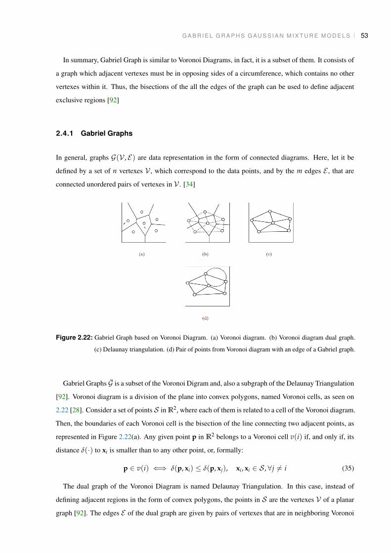
G A B R I E L G R A P H S G AU S S I A N M I X T U R E M O D E L S 53
In summary, Gabriel Graph is similar to Voronoi Diagrams, in fact, it is a subset of them. It consists of
a graph which adjacent vertexes must be in opposing sides of a circumference, which contains no other
vertexes within it. Thus, the bisections of the all the edges of the graph can be used to define adjacent
exclusive regions [92]
2.4.1 Gabriel Graphs
In general, graphs G(V , E) are data representation in the form of connected diagrams. Here, let it be
defined by a set of n vertexes V , which correspond to the data points, and by the m edges E , that are
connected unordered pairs of vertexes in V . [34]
Figure 2.22: Gabriel Graph based on Voronoi Diagram. (a) Voronoi diagram. (b) Voronoi diagram dual graph.
(c) Delaunay triangulation. (d) Pair of points from Voronoi diagram with an edge of a Gabriel graph.
Gabriel Graphs G is a subset of the Voronoi Digram and, also a subgraph of the Delaunay Triangulation
[92]. Voronoi diagram is a division of the plane into convex polygons, named Voronoi cells, as seen on
2.22 [28]. Consider a set of points S in R2, where each of them is related to a cell of the Voronoi diagram.
Then, the boundaries of each Voronoi cell is the bisection of the line connecting two adjacent points, as
represented in Figure 2.22(a). Any given point p in R2 belongs to a Voronoi cell v(i) if, and only if, its
distance δ(·) to xi is smaller than to any other point, or, formally:
p ∈ v(i) ⇐⇒ δ(p, xi) ≤ δ(p, xj), xi, xi ∈ S , ∀j 6= i (35)
The dual graph of the Voronoi Diagram is named Delaunay Triangulation. In this case, instead of
defining adjacent regions in the form of convex polygons, the points in S are the vertexes V of a planar
graph [92]. The edges E of the dual graph are given by pairs of vertexes that are in neighboring Voronoi

G A B R I E L G R A P H S G AU S S I A N M I X T U R E M O D E L S 54
cells, as seen in Figure 2.22(b). Finally, Figure 2.22(c) represents the Delaunay Trangulation resulting
from the dual of the Voronoi Diagram in Figure 2.22(a).
Gabriel graphs are an specific type of graphs within the Delaunay triangulation definition, which
allows an edge between to vertexes to exist if, and only if, an hypersphere that contains just both vertexes
and all other points are external to it, as Figure 2.22(d). Specifically, given a set of points S , a Gabriel
Graph G(V , E), with vertexes set V = S and edges set E , is defined by:
(vi, vj) ∈ E ⇐⇒ δ2(vi, vj) ≤[δ2(vi, z) + δ2(vj, z)
]∀z ∈ V , vi, vj 6= z (36)
where δ is the euclidean distance operator[92]. Thus, any types of points in space, such as geographical
coordinates, can be represented as a Gabriel Graph.
Figure 2.23: Visualization of the construction of a Gabriel Graph, in successive steps from (a) to (h). The dots are
the scattered vertexes while the edges in solid lines are being creates. Each dashed circle represents
the hypersphere of the criteria in Eq. 36
The construction of a Gabriel Graph G is represented in 2.23, where artificial data points are spatially
scattered in a plane. The G can be constructed by verifying whether each pair of points meets the premise
in Equation 36. For instance, the pairs tested in Figure 2.23 (b), (d) and (g) are connected by an edge,
but the vertexes chosen in 2.23(f) do not meet the criteria. This intuitive algorithm to construct a Gabriel
Graph has complexity order O(n3), however if the implementation is based on Delaunay triangulation,
the complexity to create the graph is O(n) [92].

G A B R I E L G R A P H S G AU S S I A N M I X T U R E M O D E L S 55
2.4.2 Geometric Parametrization of Gaussian Mixture Models
Gaussian Mixture Models are a very useful tool to define a probability density function of complex
data distributions, with appropriate choices of mean vectors µ, covariance matrix Σ and weight w of
the Gaussian functions. In geographical analysis problems, GMMs can be defined as a composition of
bivariate normal distributions, which are defined as:
P(x|µ, Σ) =1
2π |Σ|1/2 exp[−1
2(x− µ)T Σ−1 (x− µ)
]. (37)
Let the covariance matrix be given Σ = I2σ2, where I2 is a identity matrix 2× 2. Thus |Σ| = σ4 and
Σ−1 = 1/σ2, allowing the distribution to be rewritten as:
P(x|µ, σ) =1
2πσ2 exp[−1
2
(‖x− µ‖2
σ2
)]. (38)
In this case, data can be appropriately represented by a given normal distribution if it falls within
3σ of deviation around the mean µ. Consider that the probability value for x = µ + 3σ is given by
p(x|µ, Σ) = z, which is arbitrarily small with z ≈ 0. With the independent constants removed from
Equation 38, we have:
P(x|µ, σ) = exp[−1
2
(‖x− µ‖2
σ2
)], (39)
in which the σ can be isolated, resulting in
σ =
√−1
2
(‖x− µ‖2
ln(z)
), (40)
where z is the solution of Equation 38 with x = µ + 3σ, µ = 0 and σ = 1, resulting in z =
exp(−9)/2π.
Specifically in a binary classification problems, each class can be defined according to its density
distribution, enabling a the classification of unlabeled points according to its membership probability of
each class. However, an adequate selection of parameters can be a challenge as the most used method, the
Expectation Maximization, can may have some limitations[10]. In this context of binary classification,
[92] proposed a methodology to automatically select Gaussian Mixture Models parameters using Gabriel
Graphs.
In order to estimate the Gaussian Mixture Model of a Class in binary classification problems, a Gabriel
Graph is created using all available points of both classes. Then, all vertexes from one class that have
a link with the other are marked as Geometrical Vertexes GV , and the edges between them are named
Geometrical Edges GE . The GMM is, then, estimated for each class, where the centers µ are defined as
the Geometrical Vertexes of the class being estimated. Additionally, the radius are given according to
Equation 40. Finally, the weights w can be estimated through the inverse of the distance between support
vectors, also being subject to ∑j=1nG wj = 1, where nG is the number of GV .

S PAT I A L C L U S T E R I N G B A S E D O N D E L AU N AY T R I A N G U L AT I O N 56
2.5 S PAT I A L C L U S T E R I N G B A S E D O N D E L AU N AY T R I A N G U L A -
T I O N
Spatial clustering extracts information from unsupervised bidimensional data in order to create spatially
coherent clusters. In this case, the information obtained from graphs can be used to infer structural
characteristics of data [112]. In NSCABDT (Novel Spatial Clustering Algorithm Based on Delaunay
Triangulation), proposed in [112], the spatial clustering is performed using Delaunay Triangulation and
is able to discriminate clusters based on data density. The NSCABDT algorithm consists of:
1. Create Delaunay Triangulation graph D
2. Calculate the Global Mean and Standard Deviation:
Global Mean(D) =∑
j=1sum(ED)
len(ej)
sum(ED). (41)
where ED is the whole set of edges of D and len(e) are the edges lengths.
Global Sta(D) =
√√√√∑j=1ED
(Global Mean(D)− len(ej))2
sum(ED). (42)
3. For each vertex vi in D calculate:
Local Mean(vi) =∑
j=1d(vi)
len(ej)
d(vi). (43)
where d(vi) is the graph degree of each vertex and e are the edges associated with the vertex vi.
F(vi) = Global Mean(D)(
1 +Global Sta(D)Local Mean(vi)
). (44)
4. Each edge in vi that len(ei) > F(vi) is removed.
5. If d(vi) = 0 the node is discarded, else it is added to the current cluster in the clusters set C.
6. Iteratively calculate all vertex the connects do vi.
7. Extract the boundary of current cluster in C and remove bridges.
8. If no more vertexes connects to vi, repeat process with next unprocessed vertex creating a new
cluster in C until all data are processed.
The authors propose a strategy to eliminate bridges between clusters based on the effective region of
each vertex, defined by a fixed radius r around each vertex. The boundary of each cluster in C is defined
according to the border of the region formed by all the connected effective regions of the vertexes in a
cluster. The vertexes which effective region do not connected to the rest of the cluster are discarded.

3 P R O P O S E D M E T H O D S
It is change, continuing change, inevitable
change, that is the dominant factor in society
today. No sensible decision can be made any
longer without taking into account not only
the world as it is, but the world as it will be ...
Isaac Asimov, "My Own View" in The
Encyclopedia of Science Fiction (1978)
57

E S S E N T I A L LY T R A N S D U C T I V E L E A R N I N G W I T H G E N E T I C O P T I M I Z AT I O N 58
3.1 E S S E N T I A L LY T R A N S D U C T I V E L E A R N I N G W I T H G E N E T I C
O P T I M I Z AT I O N
Given that the Dataset Shift problem can be defined directly from probability distributions of the training
and testing sets, it is intuitive that the risk functional, presented in equation 1, is directly affected when
there are any type of shift. Hence, the empirical risk and the joint model error also have their values
altered on the occurrence of a shift. The use of a essentially transductive method might have the capacity
of diminishing errors in the context of Dataset Shift problems.
The essentially-trasnductive methods can be defined as binary classifiers. By minimizing the over-
all risk according to information theory methods, the said binary classifier can be estimated form the
risk function 1. If it is considered the functional (33), the problem formulation for solving essentially-
transductive learning problems takes the form of the following minimization problem:
arg min{y`+1,...,y`+k}
1k
`+k
∑i=`+1
Φ( f (xi), θ, τ),
θ = {(x1, y1), . . . , (x`, y`)},
τ = {x`+1, . . . , x`+k},
(45)
in which there is a training set θ = {(x1, y1), . . . , (x`, y`)}, a working set τ = {x`+1, . . . , x`+k}, X is
the range of the problem, and its goal is to estimate the values y`+1, . . . , y`+k associated with each point
in the working set.
The expression generalization for the continuous case has the risk asserted for the whole range of the
problem:
arg min{y`+1,...,y`+k}
∫X
Φ( f (x), θ, τ)dx,
θ = {(x1, y1), . . . , (x`, y`)},
τ = {x`+1, . . . , x`+k}.
(46)
In this continuous version, the transductive risk is not assessed at each of the given points of interest,
but over the whole range of the problem. Notice that the problem still retains its transductivity properties,
as the loss function Φ interprets and takes into consideration θ and τ, which remain discrete. Therefore,
the estimates for f (x), defined only for the points in τ (where τ ∈ χ), are given by Φ considering both
θ and τ. Hence, the solution is achieved based on the general minimum risk over the whole range of the
problem.
According to Minimum Discrimination Information principle, the Kullback-Leibler divergence be-
tween two probability distributions, may be used as discrimination information on the occurrence of new

E S S E N T I A L LY T R A N S D U C T I V E L E A R N I N G W I T H G E N E T I C O P T I M I Z AT I O N 59
facts [52]. That is, given a binary classification problem, in which classes underlying probability densi-
ties are known, the dissimilarity properties can be used to classify the unknown data according to how its
incorporation disturbs the information drawn from the known data. In this context, two strategies were
used: Minimizing the Intra-Class Information Degeneration and Maximizing Inter-Class Information
Degeneration.
3.1.1 Minimizing Intra-Class Information Degeneration
Consider a classification problem in which the classes A and B have known underlying probabilities PA
and PB, respectively. A given pattern xi should be classified considering the disturbance it causes to each
classes information, regarding its relative entropy. Thus, xi could be incorporated in either of the two
following sets, since it is a binary classification problem:
A′ = {A ∪ xi}, i = `+ 1 . . . `+ k (47)
B′ = {B ∪ xi}, i = `+ 1 . . . `+ k (48)
where A and B contain the ` labelled samples and the extended sets includes the other k samples.
With the probabilities PA and PB known already, it is possible to calculate de the information gain for
both of the classes DKL(A‖A′) and DKL(B‖B′). The sample is assigned to the class which it caused
lesser disturbance, that is, the class with smaller divergence to its extended set permanently incorporate
the new sample. The decision making rules with the Kullback-Leibler divergence is, then:
yi =
A if DKL(A‖{A ∪ xi}) < DKL(B‖{B ∪ xi}),
B if DKL(A‖{A ∪ xi}) > DKL(B‖{B ∪ xi}),
undetermined if DKL(A‖{A ∪ xi}) = DKL(B‖{B ∪ xi}),
(49)
where the undetermined values obtained at the equality may be biased to either A or B.
When we employ the Kullback-Leibler divergence and its setting given in (49) to the continuous risk
functional (46), we end up with a transductive learning method that may be solved as a multi-objective
optimization problem.
arg min{y`+1,...,y`+k}
(DKL(A(θ)‖A′(θ, τ)), DKL(B(θ)‖B′(θ, τ))),
θ = {(x1, y1), . . . , (x`, y`)},
τ = {x`+1, . . . , x`+k}.
(50)
since A and B are composed with elements in θ, and A′ and B′ also include τ.

E S S E N T I A L LY T R A N S D U C T I V E L E A R N I N G W I T H G E N E T I C O P T I M I Z AT I O N 60
To obtain a specific solution, instead of the traditional optimal Pareto front from the multi-objective
optimization, a decision maker can be created according to arbitrary bias, as defined in (49).
3.1.2 Maximizing Inter-Class Information Degeneration
If the same binary classification problem, in which the A and B classes samples have known density
distributions, occur in such manner that both classes should be the most different as possible, the model
is obtained by maximizing the dissimilarity between them. Differently from the previous approach when
the information gain between the extended sets (A′,B′) and their respective classes original distributions
(A,B) are calculated. In this case, each unlabelled sample can be assigned exclusively to one class and
the relative entropy between the extended sets A′ and B′ are calculated, regarding each other. Since, the
extended sets are mutually exclusive for the new data samples, they can be, now, represented as:
A′ = {A ∪ (xi|yi ∈ A)}, i = `+ 1 . . . `+ k (51)
B′ = {B ∪ (xi|yi ∈ B)}, i = `+ 1 . . . `+ k (52)
An estimation of yi defines the extended sets, which allows an optimization problem for the classes
divergence maximization to be given by:
arg max{y`+1,...,y`+k}
DKL(A′‖B′),
A ∪ B = {(x1, y1), . . . , (x`, y`)},
(A′ ∪ B′) = (A ∪ B) ∪ {x`+1, . . . , x`+k},
(53)
The optimization problem equation (46) can be directly transformed into the minimization problem in
(45):
arg min{y`+1,...,y`+k}
− DKL(A′(θ, τ)‖B′(θ, τ)),
θ = {(x1, y1), . . . , (x`, y`)},
τ = {x`+1, . . . , x`+k},
(54)
3.1.3 Implementation Aspects
Kulback-Leibler Divergence Objective Function
The Kullback-Leibler divergence is a measure that does not depends on parametric values of the distribu-
tion, thus, in order to provide a versatile algorithm, a Kernel Density Estimation was used to calculate the

E S S E N T I A L LY T R A N S D U C T I V E L E A R N I N G W I T H G E N E T I C O P T I M I Z AT I O N 61
probability at each point of interest, i.e. the working/testing set patterns. The KLD is, then, calculated
according to the estimated probability density and an objective function for minimization was defined
according to Algorithm 1.
Algorithm 1: Kulback-Leibler Divergence Objective Function
Data: Training set patterns and labels Xl , Yl and working set patterns Xu and estimated labels Y
Result: Objective Function f based on the negative KLD
beginKDE is calculates for all the Xu in relation to the patterns in each class
kdeA← KDE(Xu, {Xl | YL = 1} ∪
{Xu | Y = 1
})kdeB← KDE
(Xu, {Xl | YL = 0} ∪
{Xu | Y = 0
})Since the KLD is not symmetric, it was calculated for both cases
kldA ← ∑ kdeA · log(
kdeAkdeB
)kldB ← ∑ kdeB · log
(kdeBkdeA
)f ← − (kldA + kldB)
Parallel Genetic Algorithm Classification Strategy
The method implemented attempts to minimize the Kullback-Leibler divergence negative with regard
to the working/testing set labels. That is, an optimization strategy was implemented in order to define
testing/working set classification that would lead to the minimum −KLD value. Since the optimization
problem input can be defined as a bit-string and the objective function is hardly covex or unimodal, it
was decided to use an genetic algorithm approach.
However, for working/testing sets of average size the search space can increase very rapidly, since
the number of possible solutions for 2 classes is 2N , with N being the number of unlabelled patterns.
Moreover, the probability density estimation for large quantities of data can be computationally demand-
ing. Thus, it was decided to use a parallel approach, based on divide and conquer strategies. With this
approach, the working set was divided into smaller sets which were classified according to the KLD
genetic algorithm minimization. When all the subsets are classified, a greedy local search is performed
in the whole set, in order to improve the minimization starting from the solution obtained by the parallel
GA step, as shown in Algorithm 2.
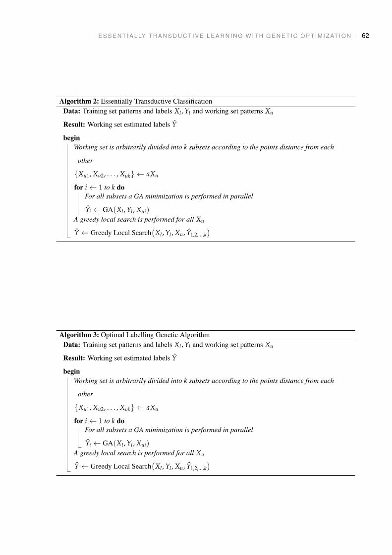
E S S E N T I A L LY T R A N S D U C T I V E L E A R N I N G W I T H G E N E T I C O P T I M I Z AT I O N 62
Algorithm 2: Essentially Transductive ClassificationData: Training set patterns and labels Xl , Yl and working set patterns Xu
Result: Working set estimated labels Y
beginWorking set is arbitrarily divided into k subsets according to the points distance from each
other
{Xu1, Xu2, . . . , Xuk} ← aXu
for i← 1 to k doFor all subsets a GA minimization is performed in parallel
Yi ← GA(Xl , Yl , Xui)
A greedy local search is performed for all Xu
Y ← Greedy Local Search(Xl , Yl , Xu, Y1,2,...,k
)
Algorithm 3: Optimal Labelling Genetic AlgorithmData: Training set patterns and labels Xl , Yl and working set patterns Xu
Result: Working set estimated labels Y
beginWorking set is arbitrarily divided into k subsets according to the points distance from each
other
{Xu1, Xu2, . . . , Xuk} ← aXu
for i← 1 to k doFor all subsets a GA minimization is performed in parallel
Yi ← GA(Xl , Yl , Xui)
A greedy local search is performed for all Xu
Y ← Greedy Local Search(Xl , Yl , Xu, Y1,2,...,k
)

T R A N S D U C T I V E A P P R O AC H B A S E D O N G A B R I E L G R A P H S 63
3.2 T R A N S D U C T I V E A P P R O AC H B A S E D O N G A B R I E L G R A P H S
Transductive learning is a intuitive approach for dataset shift and other problems where the knowledge
within the unlabelled data is relevant for the problem. For instance, in dataset shift problems, where the
training and testing sets differ, considering the unlabelled data itself to define the targets of the machine,
increase its accuracy and generalization power. Other scenarios to be considered are datasets where very
few data is unknown and/or there is severe imbalance between classes, this signifies that a very large
part of the domain main be invisible to the labelled data – the traditional training set. The transductive
approach is intrinsically capable of incorporating information from the parts of interest of the domain by
including the unlabeled data in the classification process.
As we have been studying, essentially transductive learning, however, can be very costly to classify
datasets with mare than a couple of hundred unlabeled data. The ability of training data in scenarios
where very few knowledge of the targets are known is one of the main advantages of transduction, this
characteristic is a great drawback.
Thus a different method is proposed here for bidimensional spatial datasets. This approach can be
used in a variety of real world problem that are often prone to dataset shift conditions, such as biological
and environmental data sets. The proposed method uses both labelled and unlabelled data to create
an structure that can be used to transductively label data based on the probability density of the data.
Furthermore, here is proposed a hybrid method which uses the structure used to define a semi-supervised
classifier. Thus, ultimately, the method is divided in two parts:
1. Transductive Labelling
2. Structural Classifier Selection
3.2.1 Transductive Labelling
In this first part, the main objective of the method is to attribute labels to the most significant parts of
data, through a transductive approach. Overall, probability density of data is estimated for labelled and
unlabeled data, and the labelling is performed according to dissimilarity criteria.
In this context, this methodology relies on the strategy proposed in [92] to define the density functions
through Gaussian Mixture Models using Gabriel Graphs. Since this strategy uses pairwise distance
between points, a straightforward base of comparison for all data was the use of a Delaunay Triangulation
graph based spatial clustering of unlabelled data, as proposed in [112]. This approach defines groups of

T R A N S D U C T I V E A P P R O AC H B A S E D O N G A B R I E L G R A P H S 64
data that are more likely to have the same class and discards data that can be regarded as noise and do
not consistently belong to any cluster or class.
For the labelling process, the Gaussian Mixture models are defined for the binary classes, with clusters
aggregated towards the classes. This cluster aggregation is defined according to the maximization of
Jensen-Shannon Dissimilarity between both classes. The labelling process based on entropy is favoured
by the spatial clustering, since the evaluation of the dissimilarity can be performed over clusters of data
and noise is disregarded.
In summary, the method proposed creates an unified data representation for labelled and unlabelled
data, which allows a geometrical estimation of the parameters of a Gaussian Mixture Model. Then, the
choice of ideal labels for each clusters is an optimization process that defines the maximum dissimilarity
between classes. Thereby, the structure of the Transductive Labelling is given by the Algorith 4. The
main novelty of this work is the Unified Structure T G, which was made as in Algorithm 5
With this the support vertexes are concentrated around either the points labelled in classes, case were
obtained from the GG, or around a cluster otherwise. The label of each cluster can be attributed to one
of the classes, then a density function can be estimated using the method proposed in [92]. The correct
choice of labels for each cluster can be defined according to the optimization of a statistical test, such as
minimizing Jensen-Shannon Dissimilarity.
3.2.2 Structural Classifier Selection
In order to create a classifier, a model that creates a separation surface should be implemented, which is
not in the scope of Transductive Learning. However, the proposed methodology admits noise data that
might hinder the method capability of classifying new data. Thus, the incorporation of a inductive model
at this point is interesting, since it generalizes the output for the whole input space and creates a fast
classification response for new data. In fact, any classifier algorithm could be implemented at this point,
however, in this paper, a methodology that uses the data structure already created was proposed.
In this context, the structure created to allow the Tranductive Labelling could be used to generalize
an inductive classification model based on a Bayesian approach. The classifier is obtained with the
probability density function calculated for both classes, according to the method proposed in [92]. At
this point is possible to reuse the graph structures to define the Gaussian Mixture Models. Then, a Naive
Bayes approach is used to properly define a classifier. This approach is named here as Transductive
Gabriel Graph Classifier or TGG.

T R A N S D U C T I V E A P P R O AC H B A S E D O N G A B R I E L G R A P H S 65
Algorithm 4: Transductive LabellingData: Training set patterns and labels Xl , Yl and working set patterns Xu
Result: Working set estimated labels Y
beginCreate Gabriel Graph of the labelled data based on [92]
GG ← Gabriel Graph(Xl , Yl)
Create Spatial Clusters with only unlabelled data, based on [112]
DU ← Gabriel Graph(Xu)
Create Spatial Clusters with both labelled and unlabelled data, based on [112]
DW ← Gabriel Graph(Xl , Xu)
Define unified structures to Parametrize GMMs
T G ← Unified Structure(GG,DU ,DW)
From T G is possible to extract structural information such as:
Cl ← Ordered Clusters(T G)
Nclusters ← Number of Clusters(T G)
Nclusters is limited arbitrarily and the smaller ones are considered noise
All cluster combinations are defined
Ncombination ← 2Nclusters
for i← 1 to Ncombination doFor all possible combinations the clusters receive a label
L← Binary Vector(i)
for j← 1 to Nclusters doYn ← Lj ∀ n ∈ Clj
The PDFs are calculated as in [92]
P0 ← PDF(Cl, L = 0)
P1 ← PDF(Cl, L = 1)
The dissimilarity is calculated as in 28:
JSD ← DJS(P0‖P1)
Y ← arg max(JSD)

T R A N S D U C T I V E A P P R O AC H B A S E D O N G A B R I E L G R A P H S 66
Algorithm 5: Unified StructureData: Supervised Gabriel Graph GG and Unsupervised Delaunay Triangulation Spatial Cluster
Graphs DU ,DW
Result: Unified Transductive Cluster Graph Structure T G
beginAll points that were bridges in DU and DW are considered support vertexes, analogously to
the support vertexes proposed in [92].
Both DU and DW are superposed.
All points that were considered noise or were in too small agglomerates in both DU and DW
do not have edges.
The resulting graph is superposed with GG
All points considered support vertexes in DU or DW or GG are considered support vertexes.
The prediction for this model is performed as as a simple comparison of the probability of pertinence
to each class. Since the proposed method calculates the density function for both classes, the probability
for a given point can be calculated straightforwardly for both classes and the highest one is chosen.

4 E X P E R I M E N TA L D E S I G N
It is not clear that intelligence has any long
term survival value.
Stephen Hawking, Lecture "Life in the
Universe" (1996)
67

G E N E T I C E S S E N T I A L LY T R A N S D U C T I V E L E A R N I N G E X P E R I M E N TA L D E S I G N 68
4.1 G E N E T I C E S S E N T I A L LY T R A N S D U C T I V E L E A R N I N G E X P E R -
I M E N TA L D E S I G N
The transductive approach implemented in this work is similar to semi-supervised methods, as it uses
both, labelled and unlabelled data to perform the classification. In this case, the proposed method is
expected to reach better results then supervised methods when very few labelled data is available in
comparison to the existing unlabelled data.
In this case, it is necessary to define how the amount of information in the training set affects the mod-
els robustness and performance. Therein, reducing the quantity of training data reflects on the learning
algorithm aptitude to generate an acceptable model in the presence of incomplete or inconformable data.
Furthermore, this intrinsic characteristic of using information present in unlabelled data allows robust-
ness to Dataset Shift scenarios. Thus this characteristic was tested with shifting synthetic datasets.
The proposed method should, then, be compared with popular state of the art methods, such as the
Support Vector Machine (SVM) and its semi-supervised adaptation, the Transductive Support Vector
Machine (TSVM). In this cases the methods performance was assessed for reduced training data condi-
tions for both synthetic and real-world problems.
4.1.1 Imbalanced Datasets
An important issue that is observed, specially when there are limited training patterns, is the imbalanced
dataset. Differently from the Imbalance Dataset problem presented in Section 2.1.3, the issue here relates
to the methods robustness to an imbalanced training set when no balancing technique is attempted. In
the literature there are several techniques specifically designed for treating imbalanced datasets, however
that is not the objective at this moment.
Consider, then, a scenario in which the training set and its amount of labelled patterns from each class
is uncertain, and the developer do not have much access to the labelled data itself. In this context, the
training could be performed with heavily imbalanced data. Again, in a reduced training set situation,
this imbalance causes, often, training sets with only one labelled class, which preclude most of the
usual supervised methods and a few of the accepted semi-supervised strategies. The proposed method,
however, is still permitted in this cases.
Experimental Design
Some aspects that could have some effect on the methods accuracy were considered:

G E N E T I C E S S E N T I A L LY T R A N S D U C T I V E L E A R N I N G E X P E R I M E N TA L D E S I G N 69
• Dataset.
• Quantity of training data set.
• Ration between both classes in training data (Imbalanced Data).
The tests performed in this work were intended to evaluate the methods performance when the training
data is both small and imbalanced. Actually, the imbalance analysis here is related to uncertainties in the
training, since it is desired to learn if the methods are robust to significant differences in the training set.
This robustness allows the method to work under some types of dataset drifting.
Methods Bases Ntrain Balance
ETC
SVM
TSVM
Two
moon
WBC
Hep
PID
10
5
0-10 1-9 2-8 3-7 4-6 5-5 6-4 7-3 8-2 9-1 10-0
0-5 1-4 2-3 3-2 4-1 5-0
0 10 20 30 40 50 60 70 80 90 100
x10
Rep
Figure 4.1: Diagram of the Transductive Experiment
This experimental design is represented in the diagram in Figure 4.1. The parameters of the methods
were obtained beforehand through exhaustive search.
Observe that it was chosen not to work particularly with proportions between training and work-
ing/testing sets because, in a real scenario this proportion might be unknown or, at least, harder to obtain
then the absolute amount of data.

G E N E T I C E S S E N T I A L LY T R A N S D U C T I V E L E A R N I N G E X P E R I M E N TA L D E S I G N 70
Datasets Description
The datasets used are described in Table 4.1
Table 4.1: Datasets Description
Name FeaturesPatterns
DescriptionTotal Class A Class B
Two-Moon(tmoon) 2 500 250 250 Two entangled semi-circles .
Wisconsin Breast
Cancer (wbc)
9 699 241 458 Clinical data of breast cancer di-
agnostics from the University of
Wisconsin Hospitals, Madison,
from Dr. William H. Wolberg
[11].
Hepatitis (hep) 19 155 123 32 Clinical data of Hepatites diag-
nostics.
Pima Indian Dia-
betes (hep)
19 155 123 32 Clinical data of Diabetes diag-
nostics from the National Insti-
tute of Diabetes and Digestive
and Kidney Diseases [11].
Performance metrics
In order to assess the performance of the methods the following metrics were employed:
AC C U R AC Y The accuracy is given by:
Acc =TPR + TNR
N(55)
in which N, TPR and TNR are, respectively, the total number of patterns, the true positive and the true
negative rates.
G M E A N The geometric mean is given by:
GMEAN =√
TPR× TNR (56)
in whichTPR and TNR are, respectively, the true positive and true negative rates.

G E N E T I C E S S E N T I A L LY T R A N S D U C T I V E L E A R N I N G E X P E R I M E N TA L D E S I G N 71
4.1.2 Dataset Drift
Another interesting test is the robustness in the presence of concept drifts. Some tests were performed in
order to evaluate the accuracy of the traditional Support Vector Machines, the Transductive variation of
the SVM and the proposed Essentially Transductive Learning method.
Differently from the previous one, this experiment aims to observe directly the effects of a shift in
data between training and test sets. In this scenario, off-line learning strategies are analyzed, therefore
shifted data do not have any labels. Thus this experiment assumed a very simple form, with the accuracy
analysis of the proposed method and its comparison with state-of-art methods.
Experimental Design
The experiment in this part is designed more simple. The aim of this experiment is to define the accuracy
of the methods when data provided differs between training and testing sets. Thus, the data used as
subject to Dataset Shifts.
Here, the accuracy was measured for several replications of the classification problem with shift. With
this, the variability of the method’s accuracy was affect by the variation of the differences between testing
and training distributions, as defined in equations (5) to (7). In this case the balance and size of samples
were kept equal in order to isolate the shift problem.
Methods Bases Rep
ETC
SVM
TSVM
Two
moon
Circle
Sin
x30
Figure 4.2: Diagram of the Transductive Experiment
This experimental design is represented in the diagram in Figure 4.2. The parameters of the methods
were obtained beforehand through exhaustive search.
Datasets Description
T W O M O O N The first test is a modification of the two moon dataset with the labelled data distri-
bution is biased. Here, in the labelled set, there is a greater data distribution in the central region of the
moons, which causes a covariate shift in the dataset.

G E N E T I C E S S E N T I A L LY T R A N S D U C T I V E L E A R N I N G E X P E R I M E N TA L D E S I G N 72
0.5 1 1.5 2 2.5 3 3.5 4 4.50.5
1
1.5
2
2.5
3
3.5Two Moon Drift Dataset
Class A LabeledClass B LabeledClass A UnlabeledClass B Unlabeled
Figure 4.3: Graphical representation of the Two Moon Dataset with Covariate Shift.
C I R C L E The second test is a circle which centre c and radius r differ between the labelled and the
unlabelled sets. It is based in an artificial data set containing one concept drift, proposed by [63].
S I N E The third test is a plane divided by sinusoidal wave which amplitude a, frequency f and offset
o changed between the labelled and unlabelled sets. This dataset was also proposed by [63].
Table 4.2: Description of the datasets with concept drift
Name Features
Patterns
DriftLabelled Unlabelled
Class A Class B Class A Class B
Two-Moon
(tmoon)
2 10 10 40 40 P(x)L 6= P(x)U
Circle (circ) 2 100 100 100 100 cL = [3.5, 3.5] and
rL = 0.5; cU =
[4, 4] and rU = 1
Sine (sin) 2 100 100 100 100 aL = 1, fL = 1 and
oL = 0; aU = 2,
fU = 2 and oU =
1

G A B R I E L G R A P H T R A N S D U C T I V E A P P R O AC H E X P E R I M E N TA L D E S I G N 73
4.2 G A B R I E L G R A P H T R A N S D U C T I V E A P P R O AC H E X P E R I M E N -
TA L D E S I G N
The proposed method involved two different parts, the trasnductive labelling and the proposed classifier,
thus tests were performed in order to compare:
1. The Proposed Classifier with State of Art Methods
2. State of Art Methods using and not using Transductive Labeling
The transductive labeling, at this point is deterministic and for the same data would return the same
result. Thus, in order to compare the performance of the method, different datasets were used. And for
each datasets instance used, the performance of the proposed method and of state-of-art methods with
and without transductive labeling were assessed. The design of the experiment is illustrated in Figure
4.4.
Methods Transductive Bases Rep
TGG
MLP
SVM
RBF
SVM
Poly2
TSVM
Trans.
Labels
Two
moon
Circle
Sin
Elec
x30
Figure 4.4: Diagram of the Transductive Experiment
The datasets used in this part of the experiment were the same used in 4.1.2, with the addition of the
Elec2 dataset proposed in [42], which is traditionally used in Dataset Shift Problems. However, since the
proposed method is limited to bidimensional spatial datasets, only features 4 and 6 were used.

5 E X P E R I M E N TA L R E S U LT S
True ignorance is not the absence of
knowledge, but the refuse to acquire it.
Karl Popper, As quoted by Mark Damazer in
"In Our Time’s Greatest Philosopher Vote" at
In Our Time (BBC 4)
74
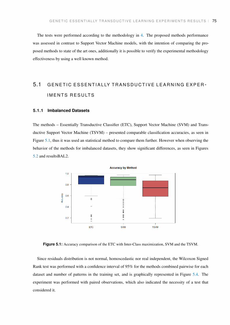
G E N E T I C E S S E N T I A L LY T R A N S D U C T I V E L E A R N I N G E X P E R I M E N T S R E S U LT S 75
The tests were performed according to the methodology in 4. The proposed methods performance
was assessed in contrast to Support Vector Machine models, with the intention of comparing the pro-
posed methods to state of the art ones, additionally it is possible to verify the experimental methodology
effectiveness by using a well known method.
5.1 G E N E T I C E S S E N T I A L LY T R A N S D U C T I V E L E A R N I N G E X P E R -
I M E N T S R E S U LT S
5.1.1 Imbalanced Datasets
The methods – Essentially Transductive Classifier (ETC), Support Vector Machine (SVM) and Trans-
ductive Support Vector Machine (TSVM) – presented comparable classification accuracies, as seen in
Figure 5.1, thus it was used an statistical method to compare them further. However when observing the
behavior of the methods for imbalanced datasets, they show significant differences, as seen in Figures
5.2 and resultsBAL2.
Figure 5.1: Accuracy comparison of the ETC with Inter-Class maximization, SVM and the TSVM.
Since residuals distribution is not normal, homoscedastic nor real independent, the Wilcoxon Signed
Rank test was performed with a confidence interval of 95% for the methods combined pairwise for each
dataset and number of patterns in the training set, and is graphically represented in Figure 5.4. The
experiment was performed with paired observations, which also indicated the necessity of a test that
considered it.

G E N E T I C E S S E N T I A L LY T R A N S D U C T I V E L E A R N I N G E X P E R I M E N T S R E S U LT S 76
ETL : 89.5+ 0.0421 x + 0.00076 x2 − 8.4e−06 x3 RMSE = 8.437574
SVM : 79.8+ 0.424 x − 0.00647 x2 + 3.28e−05 x3 RMSE = 10.31147
TSVM : 59.7+ 0.909 x − 0.0112 x2 + 1.37e−05 x3 RMSE = 16.92031
25
50
75
100
0 25 50 75 100
Balance
Acc
urac
y
Method ETC SVM TSVM
Effects SizeD_L=5
(a) Accuracy per balance for DL = 10.
ETL : 90.7+ 0.0526 x + 8e−04 x2 − 1.15e−05 x3 RMSE = 7.496279
SVM : 88.8+ 0.0564 x + 0.000527 x2 − 9.25e−06 x3 RMSE = 6.873934
TSVM : 59.6+ 0.761 x − 0.00513 x2 − 2.69e−05 x3 RMSE = 19.47188
0
25
50
75
100
0 25 50 75 100
Balance
Acc
urac
y
Method ETC SVM TSVM
Effects SizeD_L = 10
(b) Accuracy per balance for DL = 5.
Figure 5.2: Normalized Accuracy of SVM, TSVM and ETL for hepatitis, Pima Indian diabetes, Wisconsin
breast cancer and two moons datasets, with DL = 10 and 5. The balance varies from 0% (only
positive class) to 100% (only negative class) by 10% and 20% for DL = 10 and 5, respectively.
ETL : 85.4+ 0.23 x − 0.0019 x2 RMSE = 9.766729
SVM : 78.8+ 0.369 x − 0.00354 x2 RMSE = 10.13272
TSVM : 2.79+ 3.36 x − 0.0338 x2 RMSE = 11.98384
0
25
50
75
100
0 25 50 75 100
Balance
Gm
ean
Method ETC SVM TSVM
Effects SizeD_L=5
(a) GMEAN per balance for DL = 10.
ETL : 87.1+ 0.226 x − 0.00219 x2 RMSE = 9.526174
SVM : 86+ 0.216 x − 0.00225 x2 RMSE = 7.220865
TSVM : 8.1+ 3.3 x − 0.0331 x2 RMSE = 13.21422
0
25
50
75
100
0 25 50 75 100
Balance
Gm
ean
Method ETC SVM TSVM
Effects SizeD_L=10
(b) GMEAN per balance for DL = 5.
Figure 5.3: Normalized GMEAN of SVM, TSVM and ETL for hepatitis,Pima Indian diabetes, Wisconsin
breast cancer and two moons benchmark datasets, with DL equal to 10 and DL equal to 5. The
balance varies from 0% (data only from positive class) to 100% (data only from positive class) by
10% for DL = 10 and by 20% for DL = 5.
The results in Figure 5.4 indicate that, not only, all the methods results are different between each
other, since most cases failed to meet the null hypothesis that distributions were the same. But, it also
imply that if ETL approach dos not have a higher accuracy rate than the other two it is at least statistically
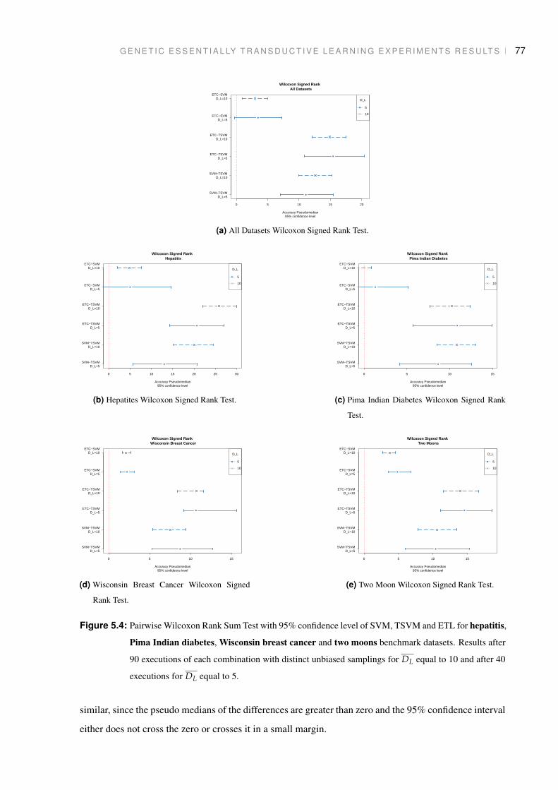
G E N E T I C E S S E N T I A L LY T R A N S D U C T I V E L E A R N I N G E X P E R I M E N T S R E S U LT S 77
0 5 10 15 20
Wilcoxon Signed Rank All Datasets
95% confidence levelAccuracy Pseudomedian
SVM−TSVMD_L=5
SVM−TSVMD_L=10
ETC−TSVMD_L=5
ETC−TSVMD_L=10
ETC−SVMD_L=5
ETC−SVMD_L=10 D_L
5
10
(a) All Datasets Wilcoxon Signed Rank Test.
0 5 10 15 20 25 30
Wilcoxon Signed Rank Hepatitis
95% confidence levelAccuracy Pseudomedian
SVM−TSVMD_L=5
SVM−TSVMD_L=10
ETC−TSVMD_L=5
ETC−TSVMD_L=10
ETC−SVMD_L=5
ETC−SVMD_L=10 D_L
5
10
(b) Hepatites Wilcoxon Signed Rank Test.
0 5 10 15
Wilcoxon Signed Rank Pima Indian Diabetes
95% confidence levelAccuracy Pseudomedian
SVM−TSVMD_L=5
SVM−TSVMD_L=10
ETC−TSVMD_L=5
ETC−TSVMD_L=10
ETC−SVMD_L=5
ETC−SVMD_L=10 D_L
5
10
(c) Pima Indian Diabetes Wilcoxon Signed Rank
Test.
0 5 10 15
Wilcoxon Signed Rank Wisconsin Breast Cancer
95% confidence levelAccuracy Pseudomedian
SVM−TSVMD_L=5
SVM−TSVMD_L=10
ETC−TSVMD_L=5
ETC−TSVMD_L=10
ETC−SVMD_L=5
ETC−SVMD_L=10 D_L
5
10
(d) Wisconsin Breast Cancer Wilcoxon Signed
Rank Test.
0 5 10 15
Wilcoxon Signed Rank Two Moons
95% confidence levelAccuracy Pseudomedian
SVM−TSVMD_L=5
SVM−TSVMD_L=10
ETC−TSVMD_L=5
ETC−TSVMD_L=10
ETC−SVMD_L=5
ETC−SVMD_L=10 D_L
5
10
(e) Two Moon Wilcoxon Signed Rank Test.
Figure 5.4: Pairwise Wilcoxon Rank Sum Test with 95% confidence level of SVM, TSVM and ETL for hepatitis,
Pima Indian diabetes, Wisconsin breast cancer and two moons benchmark datasets. Results after
90 executions of each combination with distinct unbiased samplings for DL equal to 10 and after 40
executions for DL equal to 5.
similar, since the pseudo medians of the differences are greater than zero and the 95% confidence interval
either does not cross the zero or crosses it in a small margin.

G E N E T I C E S S E N T I A L LY T R A N S D U C T I V E L E A R N I N G E X P E R I M E N T S R E S U LT S 78
5.1.2 Dataset Drift
Tests have shown that the transductive approach is intrinsically robust to drifts without the need to adap-
tive learning models. This method, that is not based in the construction of a model, is naturally capable
of classifying patterns in uncertain and restricted regions of the domain. According to Figure 5.5, the
transductive methods were always better than the SVM.
−5 0 5 10
Wilcoxon Signed Rank All Datasets
95% confidence levelAccuracy Pseudomedian
SVM−TSVM
ETC−TSVM
ETC−SVM
(a) All Datasets Wilcoxon Signed Rank Test
0 5 10 15 20
Wilcoxon Signed Rank Drift Two Moon
95% confidence levelAccuracy Pseudomedian
SVM−TSVM
ETC−TSVM
ETC−SVM
(b) Two Moons Wilcoxon Signed
Rank Test
−10 −5 0 5
Wilcoxon Signed Rank Drift Circle
95% confidence levelAccuracy Pseudomedian
SVM−TSVM
ETC−TSVM
ETC−SVM
(c) Circle Wilcoxon Signed Rank Test
−5 0 5
Wilcoxon Signed Rank Drift Sinusoidal
95% confidence levelAccuracy Pseudomedian
SVM−TSVM
ETC−TSVM
ETC−SVM
(d) Sinusoidal Wilcoxon Signed Rank
Test
Figure 5.5: Pairwise Wilcoxon Rank Sum Test with 95% confidence level of SVM, TSVM and ETL for Two
Moons, Circle and Sinusoidal benchmark datasets with Drift. Results after 30 executions of each.
These results show that the performance of different learning approaches is heavily dependent upon
the intrinsic characteristics of the data, including how much of it is available in the labeled and unlabeled
sets. Therefore, in cases where one does not wish to induce a separating margin and estimation is limited
to a given set of points known a priori, transductive learning may indeed be the best approach, although
this cannot be assumed universally for all datasets or samples.

G A B R I E L G R A P H T R A N S D U C T I V E A P P R O AC H E X P E R I M E N TA L R E S U LT S 79
5.2 G A B R I E L G R A P H T R A N S D U C T I V E A P P R O AC H E X P E R I M E N -
TA L R E S U LT S
5.2.1 Graphical Example
The method was evaluated using the following graphical bi-dimensional dataset in order to exemplify its
behaviour. This experiment allows the analysis of how the method works under the presence of dataset
shifts, with an intuitive example.
In Fig. 5.6, the resulting graph of the unified structure to calculate GMMs of the proposed strategy.
The support vertexes are marked with black circles, and is interesting to observe that the supervised
Gabriel Graph guarantees, in this case, a separation between both classes in the region defined in the
training class. Meanwhile the Spatial Clusters include support vertexes around the classes. A specific
scenario might occur when one of the classes ir highly concentrated while te other is spread throughout
the space, which is the case of the Circle dataset. In this case, the method identifies that the is a class
characterized by the data density, which allows an appropriate classification even with dataset shift. This
is possible since the method is will define the highly dense class as a single class and the other one as
noise. Fig. 5.7 and 5.8 represent DW and DU , respectively.
(a) Two Moon Dataset (b) Circle Dataset
Figure 5.6: Transductive Resulting Graph
The output of the transductive labelling is exemplified in Fig. 5.9, there the labels attributed by the
method are represented along the originally labeled ones and the resulting graph obtained in Item ??. In
this image is possible to observe the labelling according to the structure, even in a region that was not
represented in the domain of training data points.

G A B R I E L G R A P H T R A N S D U C T I V E A P P R O AC H E X P E R I M E N TA L R E S U LT S 80
(a) Two Moon Dataset (b) Circle Dataset
Figure 5.7: Spatial Cluster for Working data
(a) Two Moon Dataset (b) Circle Dataset
Figure 5.8: Spatial Cluster for Unsupervised data
(a) Two Moon Dataset (b) Circle Dataset
Figure 5.9: Transductive Labels with resulting Graph
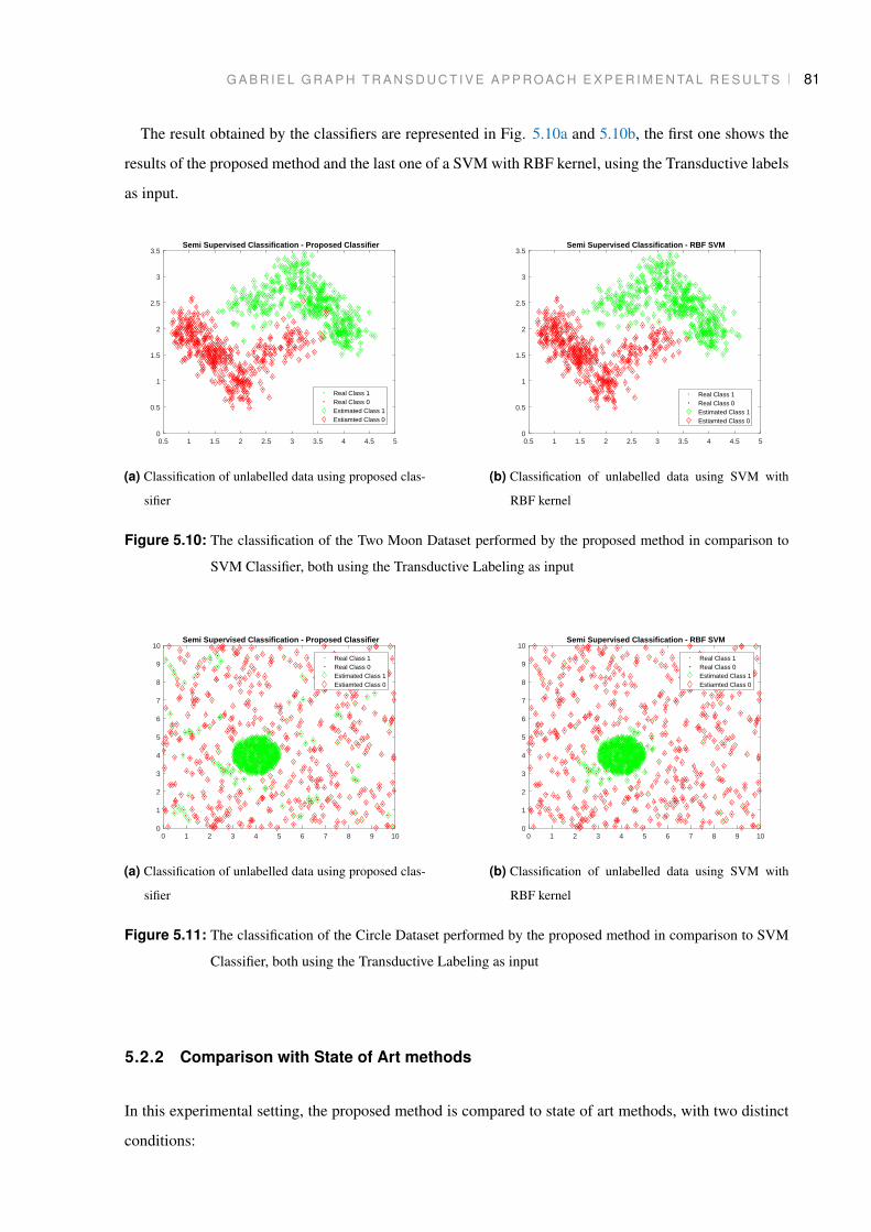
G A B R I E L G R A P H T R A N S D U C T I V E A P P R O AC H E X P E R I M E N TA L R E S U LT S 81
The result obtained by the classifiers are represented in Fig. 5.10a and 5.10b, the first one shows the
results of the proposed method and the last one of a SVM with RBF kernel, using the Transductive labels
as input.
0.5 1 1.5 2 2.5 3 3.5 4 4.5 50
0.5
1
1.5
2
2.5
3
3.5Semi Supervised Classification - Proposed Classifier
Real Class 1Real Class 0Estimated Class 1Estiamted Class 0
(a) Classification of unlabelled data using proposed clas-
sifier
0.5 1 1.5 2 2.5 3 3.5 4 4.5 50
0.5
1
1.5
2
2.5
3
3.5Semi Supervised Classification - RBF SVM
Real Class 1Real Class 0Estimated Class 1Estiamted Class 0
(b) Classification of unlabelled data using SVM with
RBF kernel
Figure 5.10: The classification of the Two Moon Dataset performed by the proposed method in comparison to
SVM Classifier, both using the Transductive Labeling as input
0 1 2 3 4 5 6 7 8 9 100
1
2
3
4
5
6
7
8
9
10Semi Supervised Classification - Proposed Classifier
Real Class 1Real Class 0Estimated Class 1Estiamted Class 0
(a) Classification of unlabelled data using proposed clas-
sifier
0 1 2 3 4 5 6 7 8 9 100
1
2
3
4
5
6
7
8
9
10Semi Supervised Classification - RBF SVM
Real Class 1Real Class 0Estimated Class 1Estiamted Class 0
(b) Classification of unlabelled data using SVM with
RBF kernel
Figure 5.11: The classification of the Circle Dataset performed by the proposed method in comparison to SVM
Classifier, both using the Transductive Labeling as input
5.2.2 Comparison with State of Art methods
In this experimental setting, the proposed method is compared to state of art methods, with two distinct
conditions:

G A B R I E L G R A P H T R A N S D U C T I V E A P P R O AC H E X P E R I M E N TA L R E S U LT S 82
1. Using the data labelled by the transductive approach to generate the classifiers.
2. Only using the originally labelled data set to generate the classifiers.
The datasets used in this experiment are the Two-Moon, shown in the previous section, the Circle
from [63] and Elec2 from [42], but since this method is intended for spatial analysis only features 4 and
6 were used. With this experiment, the improvement of classification of datasets with shift is observed
when the Transductive Labelling is applied to the whole working data. Also, it is possible to observe
that methods integrate well with this labelling strategy. Furthermore, the proposed method that uses the
labelling structure have a satisfactory behaviour in comparison to state-of-art methods, as observed in
Figure 5.12. Furthermore, it is possible to observe a significant improvement of classification when the
transductive labelling strategy is used alongside the state-of-art classifiers, as observed in Figure 5.12.
0.00
0.25
0.50
0.75
1.00
MLP SVM_Pol2 SVM_RBF TGG TSVMMethod
Acc
urac
y type
no_TL
TL
Figure 5.12: Accuracy comparison of the Transductive Gabriel Graph with State-of-Art Methods, using Trans-
ductive Labelling and Not using it, and the Transductive SVM.
In the matter of training and prediction time, Transductive approaches tend to perform much poorer
then inductive models. In this context, in Figure 5.13a it is possible to notice a slower performance of
Transductive approaches, including the TSVM that has a large ammount of outliers. Considering the
Prediction Time, the proposed classification method is slower then other state-of-art approaches, but the
hybrid solutions that are integrated with Transductive labelling have competitive performance.

G A B R I E L G R A P H T R A N S D U C T I V E A P P R O AC H E X P E R I M E N TA L R E S U LT S 83
0
100
200
300
400
500
MLP SVM_Pol2 SVM_RBF TGG TSVMMethod
Trai
n_tim
e type
no_TL
TL
(a) Training Time
0.0
0.5
1.0
1.5
MLP SVM_Pol2 SVM_RBF TGG TSVMMethod
Pre
dict
ion_
time
type
no_TL
TL
(b) Prediction Time
Figure 5.13: Computational Training and Prediction Time for the Transductive Gabriel Graph compared to State-
of-Art Methods, using Transductive Labelling and Not using it, and Transductive SVM
6 C O N C L U S I O N
We live in a society absolutely dependent on
science and technology and yet have cleverly
arranged things so that almost no one
understands science and technology. That’s a
clear prescription for disaster.
Carl Sagan and Anne Kalosh, Bringing
Science Down to Earth (1994)
84
C O N C L U S I O N 85
It was expected that the transductive approach would present a better result under situations were the
data, or real knowledge about the data distribution, is restricted. Even though the method presented
results near to the SVM, the actual rank of the classifier was higher. Regarding this comparison, there
are two main advantages of the Essentially Transductive Classifier in relation to the Support Vector
Machine Classifier. Firstly, for the used databases, the ETC presented a consistent, or at least a higher
consistency, to the classification performance for different training set imbalance configurations. This
tendency was present including cases where only a single class was presented, which is not possible with
a SVM classifier. The other advantage is that, in case of a dataset shift, a transductive approach is able
to redefine the system characteristics for the interest points during the application of the method. This
however require an appropriate memory of the data previously classified.
Furthermore, the SVM theoretically obtain results statistically close to the dataset limits for unam-
biguous classification due to its large margin optimization formulation. When the training data presented
to the SVM is reduced, the classifier margin is shifted from the optimal classification point. Thus, a
slightly better performance is, in fact, reaching small surplus open for improvement in the classification
performance.
However, the estimation of probability density of data is extremely costly to be performed at the rate
necessary tor the essentially transductive method. It required that the entropy of multiple data combina-
tions was estimated but the calculation of entropy itself needs the estimation of data probability densities.
In this case, attempts to optimize data set PDFs estimation were not successful since the problem itself
that was the target of this research is based on the deviation of the data structure from pre-setted consid-
erations. Therefore, the ETC strategy initially proposed is not scalable, resulting in prohibitively slow
performances when the datasets increased both in instances and features. Thus, the approach based in
Gabriel Graphs and spatial clustering was proposed for two dimensional data. This approach attempts
to optimization of the statistical tests, by creating a deterministic structure that can integrate both la-
belled and unlabelled data, and by predifining possible spatial clusters prior calculation of the probability
density functions, which greatly reduces the search space.
Dataset shift comprises of a large variety of problems that are a challenge to any strategy that attempts
to learn a system behaviour from data. However, this consists of a large variety of problems and, there-
fore, all cases are not likely to be all solved by a single approach. Thus, different methods have been
proposed in order to solve problems with specific contexts. In this sense, the Gabriel Graph Transductive
Approach attempts to be easily integrated to other classifiers, in order to be more easily integrated in
different applications.
The notion of the adequate similarity between classes can differ depending on the application and
type of shift, in this case the comparison between the distribution of both lasses should be adapted. In

C O N C L U S I O N 86
this context, the proposed methods are adequate for several different problems, since they use statistical
tests in order to evaluate the ideal labelling. Thus, if necessary, a different type of statistical test can be
implemented to adapt the labelling process to specific characteristics of data for problems with different
contexts.
Finally, solutions for dataset shifting still do not have any consensus and are not systematically being
used in real-world systems and applications. In the context of uncertainties in the training set, and thus
the primary assumption of dataset drift, the ETC method has shown to be an appropriate alternative of
classification learning methods, however it has shown to be a prohibitively slow method. The Gabriel
Graph Transductive Approach is a more promising method since it allows an faster transductive step and
have an structurally integrated inductive classification method, which allows faster classification of novel
data. Also, the creation of novel methods that can be easily integrated to current systems might promote
a better development of more complete solutions in the future.
Overall, dataset shift problems affects any modelling strategy that are based on data. Therefore, trans-
ductive approaches might theoretically hold some advantage since they do not attempt to define induced
general models. Instead, they generate a local transductive solution, based on all available data. However,
such approaches have great disadvantages when the time performance is considered, specially when new
data is provided, since the transductive solution must be calculated from the beginning. In this context,
hybrid solutions can be a better approach for real-world problems. In this scenario, solutions oriented to
the problems they are solving might be a more adequate strategy. Therefore, the Gabriel Graphs Trasn-
ductive Approach is an appropriate solution for specific problems with two dimensional data, such as
epidemics analysis, some images analysis, ecology, biodiversity and geology problems etc.

References
87

1 B I B L I O G R A P H Y
[1] AHAMED, T., TIAN, L., ZHANG, Y., AND TING, K. A review of remote sensing methods for
biomass feedstock production. Biomass and Bioenergy 35, 7 (2011), 2455 – 2469.
[2] ALAÍZ-RODRÍGUEZ, R., GUERRERO-CURIESES, A., AND CID-SUEIRO, J. Class and subclass
probability re-estimation to adapt a classifier in the presence of concept drift. Neurocomputing 74,
16 (2011), 2614–2623.
[3] AMARI, S.-I. Differential-Geometrical Methods in Statistics, vol. 28 of Lecture Notes in Statistics.
Springer, 1985.
[4] AMOS, B., LUDWICZUK, B., AND SATYANARAYANAN, M. Openface: A general-purpose face
recognition library with mobile applications. Tech. rep., CMU-CS-16-118, CMU School of Com-
puter Science, 2016.
[5] BÉGIN, L., GERMAIN, P., LAVIOLETTE, F., AND ROY, J. PAC-Bayesian Theory for Transduc-
tive Learning. Proceedings of the Seventeenth Conference on Antificial Intelligence and Statistics
(AISTATS) 33 (2014).
[6] BEN-DAVID, S., AND BLITZER, J. Analysis of representations for domain adaptation. In Advances
in Neural Information Processing Systems (feb 2007), vol. 19, IEEE, pp. 137–144.
[7] BENNETT, K. P., AND DEMIRIZ, A. Semi-supervised support vector machines. In Proceedings of
the 1998 Conference on Advances in Neural Information Processing Systems II (Cambridge, MA,
USA, 1999), MIT Press, pp. 368–374.
[8] BERRY, S., LEVINSOHN, J., AND PAKES, A. Differentiated products demand systems from a
combination of micro and macro data: New car market. Journ. Politic. Econ. 112, 1 (2004), 68–105.
[9] BICKEL, S., BRÜCKNER, M., AND SCHEFFER, T. Discriminative Learning Under Covariate Shift.
Journal of Machine Learning Research 10 (2009), 2137—-2155.
[10] BISHOP, C. M. Pattern Recognition and Machine Learning (Information Science and Statistics).
Springer, 2006.
[11] BLAKE, C. L., AND MERZ, C. J. UCI repository of machine learning databases, 1998.
88

B I B L I O G R A P H Y 89
[12] BRUZZONE, L., CHI, M., AND MARCONCINI, M. A novel transductive SVM for semisupervised
classification of remote-sensing images. IEEE Transactions on Geoscience and Remote Sensing 44,
11 (2006), 3363–3372.
[13] BRZEZINSKI, D., AND STEFANOWSKI, J. Prequential auc for classifier evaluation and drift de-
tection in evolving data streams. In New Frontiers in Mining Complex Patterns (2015), A. Appice,
M. Ceci, C. Loglisci, G. Manco, E. Masciari, and Z. W. Ras, Eds., Springer International Publishing,
pp. 87–101.
[14] BURGES, C. J. C. A tutorial on support vector machines for pattern recognition. Data Mining and
Knowledge Discovery 2, 2 (1998), 121–167.
[15] CAI, D., HE, X., AND HAN, J. Semi-supervised discriminant analysis. In 2007 IEEE 11th
International Conference on Computer Vision (Oct 2007), pp. 1–7.
[16] CHEN, Y., LI, W., SAKARIDIS, C., DAI, D., AND VAN GOOL, L. Domain adaptive faster r-
cnn for object detection in the wild. In IEEE Conf. Comp. Vision and Pattern Recognition (2018),
pp. 3339–3348.
[17] DA COSTA, F. G., RIOS, R. A., AND DE MELLO, R. F. Using dynamical systems tools to detect
concept drift in data streams. Expert Systems with Applications 60 (2016), 39–50.
[18] DE VITO, S., FATTORUSO, G., PARDO, M., TORTORELLA, F., AND DI FRANCIA, G. Semi-
supervised learning techniques in artificial olfaction: A novel approach to classification problems
and drift counteraction. IEEE Sensors Journal 12, 11 (2012), 3215–3224.
[19] DELANY, S. J., CUNNINGHAM, P., TSYMBAL, A., AND COYLE, L. A case-based technique for
tracking concept drift in spam filtering. Knowledge-Based Systems 18, 4-5 (2005), 187–195.
[20] DERBEKO, P., EL-YANIV, R., AND MEIR, R. Explicit learning curves for transduction and ap-
plication to clustering and compression algorithms. Journal of Artificial Intelligence Research 22, 1
(July 2004), 117–142.
[21] DHEERU, D., AND KARRA TANISKIDOU, E. UCI machine learning repository, 2017.
[22] DITZLER, G., AND POLIKAR, R. An ensemble based incremental learning framework for concept
drift and class imbalance. In 2010 International Joint Conference on Neural Networks (IJCNN) (July
2010), pp. 1–8.
[23] DITZLER, G., AND POLIKAR, R. Semi-supervised learning in nonstationary environments. In
2011 Int. Joint Conf. Neural Net. (July 2011), pp. 2741–2748.

B I B L I O G R A P H Y 90
[24] DITZLER, G., ROSEN, G., AND POLIKAR, R. Transductive learning algorithms for nonstationary
environments. In 2012 Int. Joint Conf. Neural Net. (July 2012), pp. 10–15.
[25] DITZLER, G., ROVERI, M., ALIPPI, C., AND POLIKAR, R. Learning in nonstationary environ-
ments: A survey. IEEE Computational Intelligence Magazine 10, 4 (Nov 2015), 12–25.
[26] DORNHEGE, G., BLANKERTZ, B., CURIO, G., AND MULLER, K. . Boosting bit rates in nonin-
vasive eeg single-trial classifications by feature combination and multiclass paradigms. IEEE Trans.
Bio. Eng. 51, 6 (June 2004), 993–1002.
[27] DRIES, A., AND RÜCKERT, U. Adaptive concept drift detection. Statistical Analysis and Data
Mining: The ASA Data Science Journal 2, 5-6 (2009), 311–327.
[28] DUCZMAL, L. H., MOREIRA, G. J., BURGARELLI, D., TAKAHASHI, R. H., MAGALHÃES, F. C.,
AND BODEVAN, E. C. Voronoi distance based prospective space-time scans for point data sets: a
dengue fever cluster analysis in a southeast brazilian town. International Journal of Health Geo-
graphics 10, 1 (2011), 29.
[29] ELWELL, R., AND POLIKAR, R. Incremental learning of variable rate concept drift. In Multi-
ple Classifier Systems (Berlin, Heidelberg, 2009), J. A. Benediktsson, J. Kittler, and F. Roli, Eds.,
Springer Berlin Heidelberg, pp. 142–151.
[30] ELWELL, R., AND POLIKAR, R. Incremental Learning of Concept Drift in Nonstationary Environ-
ments. IEEE Transactions on Neural Networks 22 (2011), 1517–1531.
[31] FDEZ-RIVEROLA, F., IGLESIAS, E. L., DÍAZ, F., MÉNDEZ, J. R., AND CORCHADO, J. M.
Applying lazy learning algorithms to tackle concept drift in spam filtering. Expert Systems with
Applications 33, 1 (2007), 36–48.
[32] FERNANDEZ, A., GARCIA, S., AND HERRERA, F. Addressing the Classification with Imbalanced
Data : Open Problems and New Challenges on Class Distribution In many applications , there exists a
significant difference between the class prior Addressing the Classification with Imbalanced. Hybrid
Artificial Intelligent Systems 6678 (2011), 1–10.
[33] FUGLEDE, B., AND TOPSOE, F. Jensen-shannon divergence and hilbert space embedding. In
International Symposium on Information Theory (2004), IEEE, p. 31.
[34] GABRIEL, K. R., AND SOKAL, R. R. A new statistical approach to geographic variation analysis.
Systematic Zoology 18, 3 (sep 1969), 259.

B I B L I O G R A P H Y 91
[35] GAMA, J., MEDAS, P., CASTILLO, G., AND RODRIGUES, P. Learning with drift detection. In
Advances in Artificial Intelligence – SBIA 2004 (Berlin, Heidelberg, 2004), A. L. C. Bazzan and
S. Labidi, Eds., Springer Berlin Heidelberg, pp. 286–295.
[36] GAMA, J. A., ŽLIOBAITE, I., BIFET, A., PECHENIZKIY, M., AND BOUCHACHIA, A. A survey
on concept drift adaptation. ACM Computing Surveys 46, 4 (Mar. 2014), 44:1–44:37.
[37] GAO, B., MAEKAWA, T., AMAGATA, D., AND HARA, T. Environment-adaptive malicious node
detection in manets with ensemble learning. In 2018 IEEE 38th International Conference on Dis-
tributed Computing Systems (ICDCS) (July 2018), pp. 556–566.
[38] GEMAN, S., BIENENSTOCK, E., AND DOURSAT, R. Neural Networks and the Bias/Variance
Dilemma. Neural Computation 4, 1 (Jan. 1992), 1–58.
[39] GHAZIKHANI, A., MONSEFI, R., AND SADOGHI YAZDI, H. Recursive least square perceptron
model for non-stationary and imbalanced data stream classification. Evolving Systems 4, 2 (Jun
2013), 119–131.
[40] GONZÁLEZ, P., CASTAÑO, A., CHAWLA, N. V., AND COZ, J. J. D. A review on quantification
learning. ACM Computing Surveys 50, 5 (2017), 74.
[41] HAQUE, A., KHAN, L., BARON, M., THURAISINGHAM, B., AND AGGARWAL, C. Efficient
handling of concept drift and concept evolution over Stream Data. In 2016 IEEE 32nd Int. Conf.
Data Eng. (may 2016), pp. 481–492.
[42] HARRIES, M., CSE TR, U. N., AND WALES, N. S. Splice-2 comparative evaluation: Electricity
pricing, 1999.
[43] HOFER, V., AND KREMPL, G. Drift mining in data: A framework for addressing drift in classifi-
cation. Computational Statistics & Data Analysis 57, 1 (2013), 377–391.
[44] HUANG, N. E., SHEN, Z., LONG, S. R., WU, M. C., SHIH, H. H., ZHENG, Q., YEN, N.-C.,
TUNG, C. C., AND LIU, H. H. The empirical mode decomposition and the hilbert spectrum for
nonlinear and non-stationary time series analysis. Proceedings of the Royal Society of London A:
Mathematical, Physical and Engineering Sciences 454, 1971 (1998), 903–995.
[45] KEARNS, M. J., AND VAZIRANI, U. V. An Introduction to Computational Learning Theory. MIT
Press, Cambridge, MA, USA, 1994.
[46] KHOSLA, A., ZHOU, T., MALISIEWICZ, T., EFROS, A. A., AND TORRALBA, A. Undoing the
damage of dataset bias. Lecture Notes in Computer Science (including subseries Lecture Notes in
Artificial Intelligence and Lecture Notes in Bioinformatics) 7572 LNCS (2012), 158–171.

B I B L I O G R A P H Y 92
[47] KLINKENBERG, R., AND JOACHIMS, T. Detecting concept drift with support vector machines.
In Seventeenth International Conference on Machine Learning (2000), vol. 11, Morgan Kaufmann,
pp. 487–494.
[48] KOLTER, J. Z., AND MALOOF, M. A. Dynamic weighted majority: a new ensemble method
for tracking concept drift. In Third IEEE International Conference on Data Mining (Nov 2003),
pp. 123–130.
[49] KOLTER, J. Z., AND MALOOF, M. A. Using additive expert ensembles to cope with concept drift.
In 22Nd International Conference on Machine Learning (New York, NY, USA, 2005), ICML ’05,
ACM, pp. 449–456.
[50] KONG, X., NG, M. K., AND ZHOU, Z.-H. Transductive multilabel learning via label set propaga-
tion. IEEE Transactions on Knowledge and Data Engineering 25, 3 (2013), 704–719.
[51] KULIS, B., SAENKO, K., AND DARRELL, T. What you saw is not what you get: Domain adapta-
tion using asymmetric kernel transforms. In 2011 IEEE Conference of Computer Vision and Pattern
Recognition (June 2011), IEEE, pp. 1785–1792.
[52] KULLBACK, S. Minimum discrimination information estimation and application. Tech. rep., De-
partment of Statistics, George Washington University, 1972.
[53] KULLBACK, S., AND LEIBLER, R. A. On information and sufficiency. The Annals of Mathemati-
cal Statistics 22, 1 (03 1951), 79–86.
[54] KUNCHEVA, L. I. Classifier ensembles for changing environments. In Multiple Classifier Systems
(Berlin, Heidelberg, 2004), F. Roli, J. Kittler, and T. Windeatt, Eds., Springer Berlin Heidelberg,
pp. 1–15.
[55] LI, Y., KAMBARA, H., KOIKE, Y., AND SUGIYAMA, M. Application of covariate shift adaptation
techniques in brain–computer interfaces. IEEE Trans. Bio. Eng. 57, 6 (June 2010), 1318–1324.
[56] LIN, J. Divergence measures based on the shannon entropy. IEEE Transactions on Information
theory 37, 1 (1991), 145–151.
[57] LIU, D., WU, Y., AND JIANG, H. Fp-elm: An online sequential learning algorithm for dealing
with concept drift. Neurocomputing 207 (2016), 322 – 334.
[58] LÓPEZ, V., FERNÁNDEZ, A., GARCÍA, S., PALADE, V., AND HERRERA, F. An insight into
classification with imbalanced data: Empirical results and current trends on using data intrinsic
characteristics. Information Sciences 250 (Nov. 2013), 113–141.

B I B L I O G R A P H Y 93
[59] LÓPEZ, V., FERNÁNDEZ, A., AND HERRERA, F. On the importance of the validation technique for
classification with imbalanced datasets: Addressing covariate shift when data is skewed. Information
Sciences 257 (Feb. 2014), 1–13.
[60] LOTTE, F., CONGEDO, M., LÉCUYER, A., LAMARCHE, F., AND ARNALDI, B. A review of
classification algorithms for eeg-based brain–computer interfaces. Jour. Neural Eng. 4, 2 (2007).
[61] MAIA, T. T. Aprendizado transdutivo baseado em teoria dainformação e teoria do aprendizado
estatístico. PhD thesis, UFMG School of Engineering, 7 2007.
[62] MATASCI, G., VOLPI, M., TUIA, D., AND KANEVSKI, M. F. Transfer component analysis for
domain adaptation in image classification. In Image and Signal Processing for Remote Sensing XVII
(2011).
[63] MINKU, L. L., WHITE, A. P., AND YAO, X. The impact of diversity on online ensemble learning
in the presence of concept drift. IEEE Transactions on Knowledge and Data Engineering 22, 5 (May
2010), 730–742.
[64] MINKU, L. L., AND YAO, X. Ddd: A new ensemble approach for dealing with concept drift. IEEE
Transactions on Knowledge and Data Engineering 24, 4 (April 2012), 619–633.
[65] MIRZA, B., LIN, Z., AND LIU, N. Ensemble of subset online sequential extreme learning machine
for class imbalance and concept drift. Neurocomputing 149 (2015), 316 – 329. Advances in neural
networks Advances in Extreme Learning Machines.
[66] MORENO-TORRES, J. G., LLORÀ, X., GOLDBERG, D. E., AND BHARGAVA, R. Repairing
fractures between data using genetic programming-based feature extraction: A case study in cancer
diagnosis. Information Sciences 222 (2013), 805–823.
[67] MORENO-TORRES, J. G., RAEDER, T., ALAIZ-RODRÍGUEZ, R., CHAWLA, N. V., AND HER-
RERA, F. A unifying view on dataset shift in classification. Pattern Recognition 45, 1 (Jan. 2012),
521–530.
[68] MOROSHKO, E., VAITS, N., AND CRAMMER, K. Second-order non-stationary online learning for
regression. Journal of Machine Learning Research 16 (2015), 1481–1517.
[69] NICOLAS-ALONSO, L. F., AND GOMEZ-GIL, J. Brain computer interfaces, a review. Sensors 12,
2 (2012), 1211–1279.
[70] OOMMEN, B. J., AND RUEDA, L. Stochastic learning-based weak estimation of multinomial
random variables and its applications to pattern recognition in non-stationary environments. Pattern
Recognition 39, 3 (2006), 328 – 341.

B I B L I O G R A P H Y 94
[71] PAGE, E. S. Continuous inspection schemes. Biometrika 41, 1-2 (1954), 100–115.
[72] PALHARES, D. M. F., MARCOLINO, M. S., SANTOS, T. M. M., DA SILVA, J. L. P., GOMES,
P. R., RIBEIRO, L. B., MACFARLANE, P. W., AND RIBEIRO, A. L. P. Normal limits of the
electrocardiogram derived from a large database of brazilian primary care patients. BMC Card.
Disord. 17, 1 (Jun 2017).
[73] PAN, S. J., AND YANG, Q. A Survey on Transfer Learning. IEEE Transactions on Knowledge and
Data Engineering 22, 10 (Oct. 2010), 1345–1359.
[74] PARK, S.-H., LEE, D., AND LEE, S.-G. Filter bank regularized common spatial pattern ensemble
for small sample motor imagery classification. IEEE Trans. Neural Sys. Rehab. Eng. 26, 2 (Feb
2018), 498–505.
[75] PFEFFERMANN, D., SKINNER, C. J., HOLMES, D. J., GOLDSTEIN, H., AND RASBASH, J.
Weighting for unequal selection probabilities in multilevel models. Journal of the Royal Statisti-
cal Society. Series B (Statistical Methodology) 60, 1 (1998), 23–40.
[76] POLIKAR, R. Ensemble Learning. Springer US, Boston, MA, 2012, pp. 1–34.
[77] QUIÑONERO CANDELA, J., SUGIYAMA, M., SCHWAIGHOFER, A., AND LAWRENCE, N. D.
Dataset Shift in Machine Learning. The MIT Press, Feb. 2009.
[78] RAMANATHAN, N., CHELLAPPA, R., AND BISWAS, S. Computational methods for modeling
facial aging: A survey. Jour. Vis. Lang. & Comp. 20, 3 (2009), 131 – 144.
[79] RAO, C. R. Diversity and dissimilarity coefficientes: a unified approach. Theoretical Population
Biology 21, 1 (1982), 24–43.
[80] RAZA, H., CECOTTI, H., LI, Y., AND PRASAD, G. Adaptive learning with covariate shift-
detection for motor imagery-based brain–computer interface. Soft Computing 20, 8 (Aug 2016),
3085–3096.
[81] RAZA, H., PRASAD, G., AND LI, Y. Dataset shift detection in non-stationary environments using
EWMA charts. Proceedings - 2013 IEEE International Conference on Systems, Man, and Cybernet-
ics, SMC 2013 (2013), 3151–3156.
[82] RAZA, H., PRASAD, G., AND LI, Y. EWMA model based shift-detection methods for detecting
covariate shifts in non-stationary environments. Pattern Recognition 48, 3 (Mar. 2015), 659–669.

B I B L I O G R A P H Y 95
[83] RAZA, H., PRASAD, G., LI, Y., AND CECOTTI, H. Covariate shift-adaptation using a transductive
learning model for handling non-stationarity in eeg based brain-computer interfaces. In 2014 IEEE
International Conference on Bioinformatics and Biomedicine (BIBM) (Nov 2014), pp. 230–236.
[84] RAZA, H., RATHEE, D., ZHOU, S., CECOTTI, H., AND PRASAD, G. Covariate shift estimation
based adaptive ensemble learning for handling non-stationarity in motor imagery related eeg-based
brain-computer interface. CoRR abs/1805.01044 (2018).
[85] SHEU, J.-J., CHU, K.-T., LI, N.-F., AND LEE, C.-C. An efficient incremental learning mecha-
nism for tracking concept drift in spam filtering. PLOS ONE 12, 2 (02 2017), 1–17.
[86] SHIMODAIRA, H. Improving predictive inference under covariate shift by weighting the log-
likelihood function. Journal of Statistical Planning and Inference 90 (2000), 227–244.
[87] SIAHROUDI, S. K., MOODI, P. Z., AND BEIGY, H. Detection of evolving concepts in non-
stationary data streams: A multiple kernel learning approach. Expert Systems with Applications
91 (2018), 187 – 197.
[88] SUGIYAMA, M., KRAULEDAT, M., AND MÜLLER, K.-R. Covariate Shift Adaptation by Im-
portance Weighted Cross Validation. The Journal of Machine Learning Research 8 (Dec. 2007),
985–1005.
[89] SUGIYAMA, M., NAKAJIMA, S., KASHIMA, H., BUENAU, P. V., AND KAWANABE, M. Direct
Importance Estimation with Model Selection and Its Application to Covariate Shift Adaptation. In
Advances in Neural Information Processing Systems 20 (dec 2008), J. C. Platt, D. Koller, Y. Singer,
and S. T. Roweis, Eds., Curran Associates, Inc., pp. 1433–1440.
[90] SUGIYAMA, M., AND STORKEY, A. J. Mixture Regression for Covariate Shift. In Advances in
Neural Information Processing Systems 19 (2007), B. Schölkopf, J. C. Platt, and T. Hoffman, Eds.,
MIT Press, pp. 1337–1344.
[91] TAISTER, M. A., HOLLIDAY, S. D., AND BORRMMAN, H. Computational methods for modeling
facial aging: A survey. Forensic Sci. Com. (2000).
[92] TORRES, L. C. B., CASTRO, C. L., AND BRAGA, A. P. Gabriel graph for dataset structure and
large margin classification: A bayesian approach. In Proceedings of the European Symposium on
Neural Networks (2015), pp. 237–242.
[93] TSAI, C. J., LEE, C. I., AND YANG, W. P. Mining decision rules on data streams in the presence
of concept drifts. Expert Systems with Applications 36, 2 PART 1 (2009), 1164–1178.

B I B L I O G R A P H Y 96
[94] TSYMBAL, A., PECHENIZKIY, M., CUNNINGHAM, P., AND PUURONEN, S. Dynamic integration
of classifiers for handling concept drift. Information Fusion 9, 1 (2008), 56–68.
[95] TUIA, D., PASOLLI, E., AND EMERY, W. Using active learning to adapt remote sensing image
classifiers. Remote Sensing of Environment 115, 9 (2011), 2232 – 2242.
[96] TUIA, D., PASOLLI, E., AND EMERY, W. J. Dataset shift adaptation with active queries. In 2011
Joint Urban Remote Sensing Event (April 2011), pp. 121–124.
[97] TUIA, D., PERSELLO, C., AND BRUZZONE, L. Domain adaptation for the classification of remote
sensing data: An overview of recent advances. IEEE Geosci. Remote Sens. 4, 2 (June 2016), 41–57.
[98] TURHAN, B. On the dataset shift problem in software engineering prediction models. Empirical
Software Engineering 17, 1-2 (2012), 62–74.
[99] VAPNIK, V. N. Principles of Risk Minimization for Learning Theory. Advances in Neural Infor-
mation Processing Systems 4 (1992), 831–838.
[100] VAPNIK, V. N. The nature of statistical learning theory. Springer-Verlag, jun 1995.
[101] VAPNIK, V. N. Statistical Learning Theory. John Wiley & Sons, Inc., New York, 1998.
[102] VAPNIK, V. N. An Overview of Statistical Learning Theory. IEEE Transactions on Neural
Networks 10, 5 (Sept. 1999), 988–999.
[103] WANG, H., AND ABRAHAM, Z. Concept drift detection for streaming data. In 2015 International
Joint Conference on Neural Networks (IJCNN) (July 2015), pp. 1–9.
[104] WANG, J., SHEN, X., AND PAN, W. On Transductive Support Vector Machines. Prediction and
Discovery, 1998 (2005).
[105] WANG, S., MINKU, L. L., GHEZZI, D., CALTABIANO, D., TINO, P., AND YAO, X. Concept
drift detection for online class imbalance learning. In The 2013 International Joint Conference on
Neural Networks (IJCNN) (Aug 2013), pp. 1–10.
[106] WANG, S., MINKU, L. L., AND YAO, X. Resampling-based ensemble methods for online class
imbalance learning. IEEE Transactions on Knowledge and Data Engineering 27, 5 (May 2015),
1356–1368.
[107] WANG, S., MINKU, L. L., AND YAO, X. A systematic study of online class imbalance learning
with concept drift. IEEE Transactions on Neural Networks and Learning Systems PP, 99 (2018),
1–20.

B I B L I O G R A P H Y 97
[108] WEBB, G. I., HYDE, R., CAO, H., NGUYEN, H. L., AND PETITJEAN, F. Characterizing concept
drift. Data Min. Knowl. Discov. 30, 4 (jul 2016), 964–994.
[109] WIDMER, G., AND KUBAT, M. Learning in the presence of concept drift and hidden contexts.
Machine Learning 23, 1 (1996), 69–101.
[110] WIDYANTORO, D. H., AND YEN, J. Relevant data expansion for learning concept drift from
sparsely labeled data. IEEE Transactions on Knowledge and Data Engineering 17, 3 (March 2005),
401–412.
[111] YAMADA, M., SUGIYAMA, M., AND MATSUI, T. Semi-supervised speaker identification under
covariate shift. Signal Processing 90, 8 (Aug. 2010), 2353–2361.
[112] YANG, X., AND CUI, W. A novel spatial clustering algorithm based on delaunay triangulation.
JSEA 3 (01 2010), 141–149.
[113] YUAN, C., ZHANG, Y., AND LIU, Z. A survey on technologies for automatic forest fire moni-
toring, detection, and fighting using unmanned aerial vehicles and remote sensing techniques. Can.
Journ. of Forest Res. 45, 7 (2015), 783–792.
[114] ZHANG, K., SCHÖLKOPF, B., MUANDET, K., AND WANG, Z. Domain adaptation under target
and conditional shift. In 30th International Conference on Machine Learning (2013), pp. 819–827.
[115] ZHAO, X. Face recognition algorithm based on transductive learning classifier. In Proceedings of
the 2010 International Conference on Measuring Technology and Mechatronics Automation - Volume
02 (Washington, DC, USA, 2010), ICMTMA ’10, IEEE Computer Society, pp. 212–215.
[116] ZHUKOV, A. V., SIDOROV, D. N., AND FOLEY, A. M. Random forest based approach for
concept drift handling. In Analysis of Images, Social Networks and Texts (Cham, 2017), D. I. Ignatov,
M. Y. Khachay, V. G. Labunets, N. Loukachevitch, S. I. Nikolenko, A. Panchenko, A. V. Savchenko,
and K. Vorontsov, Eds., pp. 69–77.
[117] ŽLIOBAITE, I., BIFET, A., PFAHRINGER, B., AND HOLMES, G. Active learning with drifting
streaming data. IEEE Transactions on Neural Networks and Learning Systems 25, 1 (Jan 2014),
27–39.
[118] ŽLIOBAITE, I., PECHENIZKIY, M., AND GAMA, J. An Overview of Concept Drift Applications.
Springer International Publishing, 2016, pp. 91–114.