Transactions Papers A View of Gaussian Elimination Applied ...

IEEE TRANSACTIONS ON COMMUNICATIONS, VOL. 55, NO. 6, JUNE 2007 1131

Transactions Papers

A View of Gaussian Elimination Applied toEarly-Stopped Berlekamp–Massey Algorithm

Chih-Wei Liu, Member, IEEE, and Chung-Chin Lu, Member, IEEE

Abstract—In this paper, we adopt a restricted Gaussian elimi-nation on the Hankel structured augmented syndrome matrix toreinterpret an early-stopped version of the Berlekamp–Massey al-gorithm in which only ( + ) iterations are needed to be per-formed for the decoding of BCH codes up to errors, where isthe number of errors actually occurred with , instead of the2 iterations required in the conventional Berlekamp–Massey al-gorithm. The minimality of ( + ) iterations in this early-stoppedBerlekamp–Massey (ESBM) algorithm is justified and related tothe subject of simultaneous error correction and detection in thispaper. We show that the multiplicative complexity of the ESBM al-gorithm is upper bounded by ( + 2 1) and except fora trivial case, the ESBM algorithm is the most efficient algorithmfor finding the error-locator polynomial.

Index Terms—BCH codes, Berlekamp–Massey algorithm, de-coding, error-correcting codes, Gaussian elimination.

I. INTRODUCTION

LET , be the syndromes for a transmittedcodeword of a BCH code with design error-correcting ca-

pability . Suppose there are exactly errors, . The coeffi-cients of the error-locator polynomial with

satisfy [4]–[6]

(1)

With its low complexity of order , the Berlekamp–Masseyalgorithm is one of the most popular algorithms for computingthe error-locator polynomial. The Berlekamp–Massey algo-rithm, as discussed in [7] and [8] interprets the linear recurrencein (1) as a shift-register synthesis problem. The determinationof the error-locator polynomial then becomes the synthesisof a minimum-length linear-feedback shift register (LFSR)to generate a known, prescribed sequence of syndromes. Ingeneralizing the Berlekamp–Massey algorithm to decode cycliccodes up to the Hartmann–Tzeng bound and the Ross bound

Paper approved by T.-K. Truong, the Editor for Coding Theory and Tech-niques of the IEEE Communications Society. Manuscript received August 21,2004; revised July 28, 2006. This work was supported by the National ScienceCouncil, Taiwan, R.O.C., under Contract NSC89-2213-E-007-060.

C.-W. Liu is with the Department of Electronics Engineering, National ChiaoTung University, Hsinchu 30010, Taiwan, R.O.C.

C.-C. Lu is with the Department of Electrical Engineering, National TsingHua University, Hsinchu 30013, Taiwan, R.O.C.

Digital Object Identifier 10.1109/TCOMM.2007.898827

in [1], the determination of the error-locator polynomial isreformulated as the problem of finding the smallest initial set oflinearly dependent columns in a matrix formed by syndromes.An algorithm, called the fundamental iterative algorithm (FIA),which is a kind of restricted Gaussian elimination, is proposedin [1] to solve the problem of finding the smallest initial setof linearly dependent columns in a generic matrix. It is shownthere that the Berlekamp–Massey algorithm is equivalent to arefinement of the FIA on a syndrome matrix of the form

......

. . ....

...(2)

where the entries , , designate “don’tcares” and can be so specified as to satisfy the linear dependencerelation in (1).

However, a more efficient version of the Berlekamp–Masseyalgorithm is developed in [2] and [3] and requires onlyiterations to be performed for the decoding of BCH codes upto errors, where is the number of errors actually occurredwith , instead of the iterations in the conventionalBerlekamp–Massey algorithm.

To begin with our excursion from the Gaussian eliminationto this early-stopped Berlekamp–Massey (ESBM) algorithm, itturns out that the syndrome matrix in (2) is too big to betaken. To present a syndrome matrix of the right size as hinted in[2], we first state the following basic theorem which is the foun-dation of the Gorenstein–Zierler decoding method. For a proofof this theorem, please see [9] or any of the textbooks in [4]–[6].

Theorem 1: Suppose that the number of errors actually oc-curred is and . Then the syndrome matrix ,where

......

. . ....

is nonsingular if and singular if .This theorem leads naturally to a top-down approach, begin-

ning with the matrix and ending with the matrix , tocheck their nonsingularity in order to determine the number oferrors actually occurred, provided that (see [4]), and after

0090-6778/$25.00 © 2007 IEEE

1132 IEEE TRANSACTIONS ON COMMUNICATIONS, VOL. 55, NO. 6, JUNE 2007

the nonsingular square matrix stands out, the followingmatrix equation:

......

can be solved by applying Gaussian elimination first and thenbackward substitution on the augmented syndromematrix

......

. . ....

...

Now, for a bottom-up approach, consider the maximal pos-sible augmented syndrome matrix

......

. . ....

...(3)

From (1), the th column of is a linear combinationof its previous (left) columns, i.e.,

(4)

for each , . On the other hand, the firstcolumns of are linearly independent since the principalsubmatrix of is nonsingular by Theorem 1 and thenthe columns of are linearly independent. Furthermore,the expression of the th column of as a linearcombination of the first columns of , , as in (4)must be unique, i.e., the coefficients ’s of the error-locatorpolynomial can be uniquely determined once the first (i.e., the

th) column of is expressed as a linear combination ofits previous columns in . We summarize the above discussionin the following corollary.

Collorary 2: Suppose that the number of errors actually oc-curred is and . Then the first column of the augmentedsyndrome matrix being a linear combination of its previouscolumns is , and the linear combination coefficients deter-mine the error-locator polynomial.

A variant of Gaussian elimination on the rows of the aug-mented syndrome matrix in (3) is adopted in [10] to determinethe coefficients of the error-locator polynomial. Although thisalgorithm is shown to be more efficient than the conventionalBerlekamp–Massey algorithm when the number of errors ac-tually occurred is very small, it is still subject to the same highcomplexity of order as the Gaussian elimination operateson a generic matrix of dimension . This is because that the rowoperations are not the right operations to be performed on theaugmented syndrome matrix and the structural properties ofthe augmented syndrome matrix are not exploited there.

Structural properties of other syndrome matrices than areexploited implicitly in [1] and more explicitly in [11] in the

derivation of the Berlekamp–Massey algorithm. In [11], var-ious syndrome matrices, being identified as Hankel matrices,are used to derive an inherent rule of how the length of theminimal LFSR, synthesized by an arbitrary recursive algorithm(including the Berlekamp–Massey algorithm), grows with thelength of the syndrome sequence input to the algorithm. A nec-essary and sufficient condition of the uniqueness of the LFSRis derived there, and the early-stopped conditions in [2] and [3]for the Berlekamp–Massey algorithm are also revisited in [11].

In this paper, we will adopt the right type of column opera-tions, a restricted Gaussian elimination as that in the FIA in [1],to perform on the right augmented syndrome matrix in (3) withthe exploitation of the structural properties of . With this newapproach, we will develop an ESBM algorithm, as a re-interpre-tation of the early-stopped version of the Berlekamp–Masseyalgorithm in [2] and [3], in which only iterations areneeded to be performed for the decoding of BCH codes up toerrors, where is the number of errors actually occurred with

, instead of the iterations required in the conventionalBerlekamp–Massey algorithm. Although an attempt to show theminimality of iterations in an ESBM algorithm is madein [11], we think it is vague and not successful. We will provethe minimality of iterations through our formulationand relate it to the subject of simultaneous error correction anddetection. We will analyze the multiplicative complexity of thedeveloped algorithm and show that except one trivial case, ourdeveloped ESBM algorithm is the most efficient algorithm forfinding the error-locator polynomial.

II. LEFT-COLUMN REPLACEMENT OPERATIONS

In this section, we will present a basic type of column oper-ations performed in the fundamental iterative algorithm (FIA)in [1] for determining the linear dependency of a column on itsprevious (i.e., left) columns in a matrix. Related concepts anduseful results will be further developed.

To determine the linear dependency of a column on its pre-vious columns in a matrix , a restricted Gaussian eliminationon columns of can be performed as follows. For each nonzerocolumn of , we add a multiple of a previous column ,

, of from column to eliminate the leading (i.e., top-most) nonzero entry of column to lower down the positionof the leading nonzero entry of the newly resulted column, ifpossible. More precisely, if the leading nonzero entry of the thcolumn is the th entry and there is a previous column

, , which has a leading nonzero entry also at theth position, then we replace column by .

The replaced column is either a zero vectoror has a leading nonzero entry below the th position. Such anelimination operation is called a left-column replacement oper-ation. A matrix is called a left-reduced matrix of if it isobtained by applying a series of left-column replacement oper-ations on and the leading nonzero entry of each column of

, if exists, cannot be further eliminated by any left-columnreplacement operation. The leading nonzero entry of a columnin a left-reduced matrix is called a pivot. Pivots must be indifferent rows of ; otherwise, one of them can be further elim-inated by a left-column replacement operation.

LIU AND LU: VIEW OF GAUSSIAN ELIMINATION APPLIED TO EARLY-STOPPED BERLEKAMP–MASSEY ALGORITHM 1133

It is clear that each column of a left-reduced matrix isa linear combination of the first columns , , ofthe original matrix as

(5)

where , , are constants and dependent on thecolumn index . If of the left-reduced matrix is a zerovector, then column of the original matrix is a linear com-bination of its previous columns in . Otherwise, column hasa pivot at the th coordinate for some . Since

, we have

(6)

from (5) and column of is said to be a partial linear combi-nation of its previous columns up to the th entry. A furtherargument can render us the following lemma.

Lemma 3: A left-reduced matrix of a matrix has a pivotat the th position if and only if the th column of is apartial linear combination of its previous columns in up tothe th entry, but not to the th entry.

Proof: Please see Appendix I.Thus, all left-reduced matrices of a matrix have the same

pivot positions and we shall say that the matrix has a pivotposition at the th entry if a left-reduced matrix of has apivot at that position. A consequence of Lemma 3 is that matrix

has a pivot position in column if and only if column islinearly independent of its previous columns in .

Recall that a square matrix is symmetric if forall . The following lemma is useful later.

Lemma 4: A square symmetric matrix has a pivot positionat the th entry if and only if it has a pivot position at thetransposed th entry.

Proof: Please see Appendix II.

III. STRUCTURAL PROPERTIES OF THE AUGMENTED

SYNDROME MATRIX

In this section, we assume that the number of errors actu-ally occurred is no greater than . By Corollary 2, the last (i.e.,the th) column of the augmented syndrome matrix

in (3) is a linear combination of its previous columns, and byLemma 3, all pivot positions of are located in the principalsubmatrix which is square and symmetric. The next corol-lary follows from Lemma 4.

Corollary 5: If the number of errors actually occurred isno greater than , then the augmented syndrome matrix hasa pivot position at the th entry if and only if it has a pivotposition at the transposed th entry.

An matrix is said to be in a Hankel form if(7)

The augmented syndrome matrix in (3) is in a Hankel formsince the th entry of is for all ,

. The slanted diagonal in where all ’s reside,as shown in Fig. 1 for , is called the -slanteddiagonal. While for each , , the -slanted

Fig. 1. S -slanted diagonal and the S -slanted diagonal in the augmentedsyndrome matrix SSS.

diagonal does not cross the first columns of , we shallstill regard every entry in these columns as being abovethe -slanted diagonal.

Lemma 6: Given an , , if a column of has apivot position on or above the -slanted diagonal, then everycolumn of to the left of that column also has a pivot positionon or above the -slanted diagonal.

Proof: Let the column having a pivot position on or abovethe -slanted diagonal be the th column . If , weare done. Suppose that and that there is a column ,

, which does not have any pivot position on or abovethe -slanted diagonal. If , i.e., all entries of thecolumn are above the -slanted diagonal, then the column

of the augmented syndrome matrix is a linear combinationof its previous columns by Lemma 3. Thus, by Corollary 2, wehave . Hence, since , the columnis also a linear combination of its previous columns in andthen does not have any pivot position by Lemma 3, which is acontradiction. Thus, and the column is a partiallinear combination of its previous columns in up to the

th entry by Lemma 3. Then there exist coefficients, , such that

(8)

Since is in a Hankel form and by (7), we havefor all ,

. With and from (8), we have

which means that the column is a partial linear combinationof its previous columns in up to the th entry ,which is on the -slanted diagonal, a contradiction, too. Thiscompletes the proof.

Now, for each , , we define to be the columnindex of the rightmost column in which has a pivot position onor above the -slanted diagonal. If there does not exist such acolumn, we define to be 0. It is clear that the first columnsof the augmented syndrome matrix are linearly independentand the th column of is a partial linear combinationof its previous columns up to the th entry . Let bethe first such that

(9)


Then the th column is the first column which is a linearcombination of its previous columns in , and by Corollary 2,we have and then

(10)

If , then trivially. Now suppose that. Since the column of has a pivot position on

or above the -slanted diagonal which is trivially above the-slanted diagonal, we have

(11)

Lemma 7: For an , , with , the principalsubmatrix of is nonsingular. In particular, there are

pivot positions of within the submatrix which arein different columns and in different rows.

Proof: By Lemma 6, each column , , of hasa pivot position on or above the -slanted diagonal. Thus, thefirst columns of are linearly independent. Suppose thatthere is a column, says column , , with pivot positionlocated below the th entry, says located at the th entry. Thenwe have which implies .By the symmetry property of the pivot positions in , as statedin Corollary 5, the column of has a pivot position whichis located at the th entry, i.e., the th position of . With

, this pivot position (i.e., the th entry) of columnis on or above the -slanted diagonal, which contradicts

to the definition of . Thus, the pivot position in each of thefirst (linearly independent) columns of is located on orabove the th entry. Hence, there are pivot positions oflocated within the principal submatrix of , which arein different columns and in different rows. It is clear that thissubmatrix is nonsingular.

Suppose that . Since the submatrix ofis nonsingular by Lemma 7, any vector of dimension

must be a linear combination of the columns in .Thus, each column , , of is a partiallinear combination of its previous columns in up to the thentry . The smallest , ,such that (which means that the column

is a partial linear combination of its previous columns up toan entry on or below the -slanted diagonal and then cannothave a pivot position on or above the -slanted diagonal) is

. This implies that

(12)

by Lemma 6. Thus, if , i.e., , thenwe have from (11) and (12). Now suppose that

, i.e., . If , then all entries ofthe column are on or above the -slanted diagonaland by the definition of , the column is a linearcombination of its previous columns in . By Corollary 2, everycolumn of to the right of the column is also a linearcombination of its previous columns in . Thus, we have

and then by (11). Now consider. If the column is a partial linear combination of its

previous columns up to the th entry , then it is clearthat by Lemma 6 and then by (11). If

not, the column has a pivot position at the thentry , and by Corollary 5, the column has a pivotposition at the th entry . Now, by Lemma 6, wehave and then by (12). Wesummarize the results in the following theorem, where we let

for convenience.Theorem 8: For or , we have

, and for , if the columnis a partial linear combination of its previous columns

up to the th entry , then and if not,.

From (11), the sequence is nonde-creasing. The next corollary describes the pattern of pivotpositions in the augmented syndrome matrix .

Collorary 9: If , then there does not exist anypivot position of on the -slanted diagonal, and if

, then there are exactly pivot positions of lyingon the -slanted diagonal, beginning at the thentry and ending up at the th entry.

Proof: By Lemma 6, each of the first columns of hasa pivot position on or above the -slanted diagonal and noneof the rest columns have a pivot position on or abovethe -slanted diagonal. Thus, if , then there doesnot exist any pivot position of on the -slanted diagonal.Now for , we have and

by Theorem 8. Then the -slanted diagonalcrosses the column at the th entry

up to the column at the th entry . Thus,there are exactly pivot positions of lying on the

-slanted diagonal, beginning at the th entryand ending up at the th entry. This completes theproof.

IV. EARLY-STOPPED BERLEKAMP–MASSEY

(ESBM) ALGORITHM

Suppose that there are jumps in the nondecreasing sequenceat indices , , i.e.,

if and otherwise, where we have definedfor convenience. From Theorem 8, we have

(13)

Let be the size of the jump at . ByCorollary 9, is the number of (consecutive) pivot positions of

lying on the -slanted diagonal and there is no pivot positionof lying on the -slanted diagonal if is not a jump index.Then we have

(14)

and, in particular, by assuming that the number of errors ac-tually occurred is no greater than , the total number of pivotpositions in is from Corollary 2, and we have

(15)

Since the principal submatrix of for each ,, is nonsingular by Lemma 7, the th column of


is a linear combination of its previous columns in up tothe th entry , i.e.,

(16)

where the linear combination coefficient vector

must be unique (We will use a

-tuple, denoted by , with the rightmost component to be 1to represent the coefficients of a linear combination with whichthe th column is a partial linear combination of its previouscolumns up to the th component as in above. In general, isnot necessarily unique). We next describe an iterative procedure

to find , , and from , , and .To find the next jump index , and then , is equivalent

to find the , beginning at and ending at, such that the th column of

is not a partial linear combination of its previous columns up tothe th entry by Theorem 8, i.e., to find the firstin such that the discrepancy

(17)

is nonzero by Lemma 3. This is called the search phase forand then for .

If all the discrepancies , ,are zeros, then the th column is thefirst column of which is a linear combination of its pre-vious columns. By Corollary 2, the linear combination co-

efficient vector is equal to the coefficient vector

of the error-locator polynomial andno more pivot positions of can be found. In this case, the finalindex has and such thatthis final index is the first index with and .By (9), this final index is equal to . Thus, no more jumpindex can be found, and we have . Otherwise, we find

as the first in with . Thiscompletes the phase of search for , and then we have

(18)

as stated in Theorem 8.Now, to determine the linear combination coefficient vector

with which the th column of is aunique linear combination of its previous columns in upto the th entry , we will apply left-column replacementoperations on the augmented syndrome matrix . This is called

the update phase for .

At first, we note that the th column of is a linearcombination of its previous columns in up to the

th entry , i.e.,

for all , , since the discrepancy in(17) is zero from to . Now sinceis in a Hankel form, we have

for all , , i.e.,

for all , , which says that the thcolumn of is a linear combination of its previous columns in

up to the th entry with linear combinationcoefficient vector

(19)

Since

from (17), and there is a pivot position at theth entry (i.e., the th entry since

by (18)) of , i.e.,

we have

This implies that the th column of is a partiallinear combination of its previous columns in up to the


Fig. 2. Alternative search and update phases in the iteration process of deter-

mining r , L and�� for j = 1; 2; . . . ; J , where the pivot positions aremarked by “�.”

th entry with the linear combination coefficient vector

by updating the vector to

(20)

by (19), which is, indeed, the result via a series of left-columnreplacement operations on to eliminate all nonzero entries ator above the th position of the th column

of .Now for each , , we continue

to eliminate the th entry of the th columnby employing the pivot at the thposition, lying on the -slanted diagonal as stated in Corollary

9, and by updating the vector to

(21)where

(22)

After completing the phase of updating coefficient vector at, we obtain the desired linear combination coefficient

vector , which is unique.We now summarize the iterative procedure to find , and

as shown in Fig. 2. In general, there are two phases ineach th iteration. The first phase is a search phase for in theinterval of the index by detecting a

nonzero discrepancy in (17) by using the most recently ob-

tained linear combination coefficient vector . If none

of the discrepancies with isdetected to be nonzero, then the number of errors actually oc-curred is and the coefficient vector of the error-locator

polynomial is . Then the algorithm stops. Oth-erwise, is found and . The end of the firstphase triggers immediately the begin of the second phase. Thesecond phase is an update phase for obtaining the next linear

combination coefficient vector in the intervalof the index . We use (20) to update the coefficient vector when

and use (21) when .There are totally iterations and the last, i.e., the th,

iteration consists of only a search phase. For each , ,the th iteration consists of steps for theindex from to . Among the steps, the first

steps for the index from to is in theth search phase and the last steps for the index from

to is in the th update phase. Note that theth search phase and the th update phase overlap at the th

step of the th iteration for the index ,where the th jump of the sequence occurs.In each step of the th iteration, we should at first calculate thediscrepancy by (17) or (22), depending on the index beingin the search phase or in the update phase. Since

(23)

we have

(24)

by (17), (20), and (21). Thus, we can rewrite the calculation ofthe th discrepancy as

(25)

by (17), (22), and (24). Since the discrepancy is zero in thesearch phase except at the last step, i.e., the th step, there isno need to update the linear combination coefficient vector. Asimilar case occurs if the discrepancy is zero in the updatephase. However, if the discrepancy is nonzero in the updatephase except at the first step, i.e., the th step, we will updatethe linear combination coefficient vector as

(26)

for , where we have used two auxiliaryvariables

(27)

(28)

by (21) and (24) and the notation for a vectorin (26) with , is defined to be the right

-truncate of the vector , i.e., .


Now, when , the discrepancy is nonzero and the linearcombination coefficient vector will be updated as

(29)

where

(30)

(31)

by (20) and (24). From (27) and (30), we have

(32)

and from (28) and (31), we have

.(33)

With (23), (26), (29), (32), and (33), we now write a pseu-docode for the procedure in above, based on the index of thesyndromes , . In the pseudocode, the fol-lowing variables are used.

To store the index of the rightmost columnin which has a pivot position on or above the

-slanted diagonal.

To store the coefficient vector with whichthe th column of is a partial linearcombination of its previous columns up to the

th component .To store the pivot value to be used to update thecoefficient vector to eliminate the thentry .To store the linear combination coefficient vector

associated with the pivot in above to be usedto update the coefficient vector to eliminate the

th entry .To store the linear combination coefficient vector

temporarily for later use.

Since the algorithm begins in searching for a nonzero entry (i.e.,a pivot position) in the first column of the augmented syndromematrix , the initial values of the first four variables are set to be

and (34)

For from 1 to

Calculate of by ;

If and

/ at the end of the last search phase /

;

;

the algorithm stops.

Else if

/ either in a search phase or in an update phase /

[by (33)].

Else if and

/ in an update phase but not in a search phase /

[by (26)];

[by (33)].

Else if and

/ at the overlap of a search & an update phases /

[by(29)];

[by (33)];

[by (32)];

[by (23)].

The algorithm in above is equivalent to the modifiedBerlekamp–Massey algorithm in [2], which is the same as theconventional Berlekamp–Massey algorithm in [7] and [8] ex-cept for the detection of an early stop by the conditionsand . However, the distinction between the algorithmdeveloped in above and the modified Berlekamp–Massey al-gorithm in [2] stems from the distinction between the refinedFIA in [1] and the conventional Berlekamp–Massey algorithmin [7] and [8]. Moreover, while Hankel properties of varioussyndrome matrices are exploited in [11], the manipulation ofsyndrome matrices in [11] remains the style of the conven-tional Berlekamp–Massey algorithm. While the conventionalBerlekamp–Massey algorithm is shown to be equivalent to arefinement of FIA in [1], the refined FIA has lower complexitythan the conventional Berlekamp–Massey algorithm as can beseen in Section VI. Thus, the developed algorithm in above haslower complexity than the modified Berlekamp–Massey algo-rithm in [2]. This algorithm will be referred as the ESBM algo-rithm. From (9) and (10), the algorithm stops at .Thus, only iterations are needed to be performed in theESBM algorithm for the decoding of BCH codes up to errors,where is the number of errors actually occurred with ,instead of the constant iterations required in the conventionalBerlekamp–Massey algorithm. Note that in the completion ofthe ESBM algorithm, stores the linear combination coeffi-

cient vector and theerror-locator polynomial is

A scenario of the execution of the ESBM algorithm is illus-trated in Fig. 3, where there are errors actually oc-curred in the decoding of a codeword from a BCH code witherror-correcting capability . In Fig. 3, the progression of


Fig. 3. Illustrative scenario of applying the ESBM algorithm to the decoding of a BCH code with designed error-correcting capability t = 16 for the case ofe = 10 errors occurred.

the index of the syndrome sequenceis described in an alternative search and update phases mannerand all the pivot positions of the augmented syndrome matrixare marked by “ .” Suppose further that there are four jumps,i.e., , occurred at , , , and ,respectively. Then , ,

, and , and ,, , .

The first search phase begins at the step of to detect anonzero discrepancy up to the step of in the first columnof . Since , i.e., , the first search phase ends at thestep of and then , . The first update phaseis triggered immediately but without doing anything at the stepof , as by setting the initial value of to be 0, since the

-slanted diagonal is above the second column of , i.e., thesecond column does not have as an entry. The first updatephase ends at the step of with , wherethe execution of an update of the linear combination coefficientvector depends on whether the discrepancy is zero or not.

The second search phase begins at the step ofto detect a nonzero discrepancy up to the step of

in the th column of . Sinceand , the second search phase ends

at the step of and then , . The secondupdate phase is triggered immediately for updating the linearcombination coefficient vector to eliminate the nonzero leadingentries of the th column of , when the discrepancy

is nonzero, up to the th entry for the step indexfrom to .

Similar operations are done in the third and the fourth itera-tions, which are from the step of to the step ofand from the step of to the step of respectively.We have , and , , and the fifthsearch phase begins at the step of to detecta nonzero discrepancy up to the step of inthe th column of . Since ,we detect an early stop of the algorithm such that the numberof errors actually occurred is .


It is now clear that the algorithm stops at the step ofwhich is really six steps earlier than the

conventional Berlekamp–Massey algorithm which stops at thestep of .

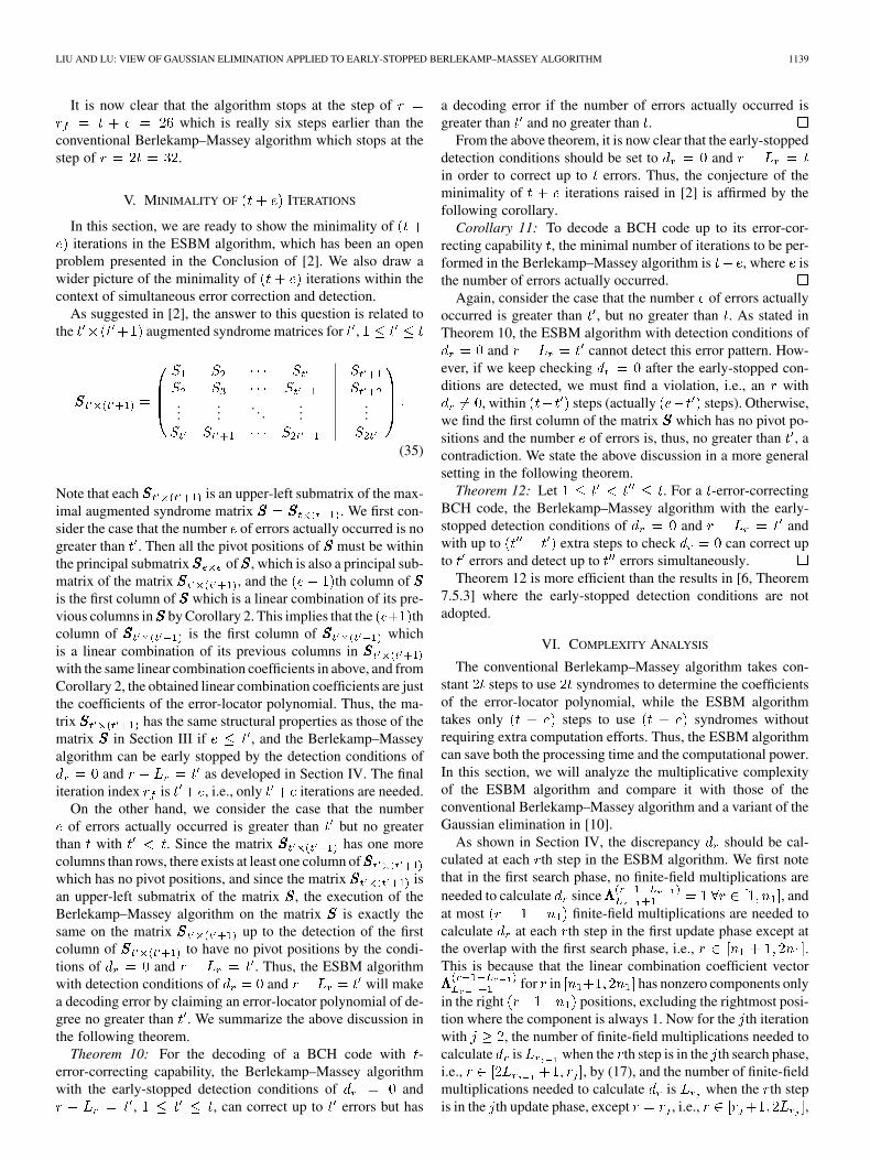
V. MINIMALITY OF ITERATIONS

In this section, we are ready to show the minimality ofiterations in the ESBM algorithm, which has been an open

problem presented in the Conclusion of [2]. We also draw awider picture of the minimality of iterations within thecontext of simultaneous error correction and detection.

As suggested in [2], the answer to this question is related tothe augmented syndrome matrices for ,

......

. . ....

...

(35)

Note that each is an upper-left submatrix of the max-imal augmented syndrome matrix . We first con-sider the case that the number of errors actually occurred is nogreater than . Then all the pivot positions of must be withinthe principal submatrix of , which is also a principal sub-matrix of the matrix , and the th column ofis the first column of which is a linear combination of its pre-vious columns in by Corollary 2. This implies that the thcolumn of is the first column of whichis a linear combination of its previous columns inwith the same linear combination coefficients in above, and fromCorollary 2, the obtained linear combination coefficients are justthe coefficients of the error-locator polynomial. Thus, the ma-trix has the same structural properties as those of thematrix in Section III if , and the Berlekamp–Masseyalgorithm can be early stopped by the detection conditions of

and as developed in Section IV. The finaliteration index is , i.e., only iterations are needed.

On the other hand, we consider the case that the numberof errors actually occurred is greater than but no greater

than with . Since the matrix has one morecolumns than rows, there exists at least one column ofwhich has no pivot positions, and since the matrix isan upper-left submatrix of the matrix , the execution of theBerlekamp–Massey algorithm on the matrix is exactly thesame on the matrix up to the detection of the firstcolumn of to have no pivot positions by the condi-tions of and . Thus, the ESBM algorithmwith detection conditions of and will makea decoding error by claiming an error-locator polynomial of de-gree no greater than . We summarize the above discussion inthe following theorem.

Theorem 10: For the decoding of a BCH code with -error-correcting capability, the Berlekamp–Massey algorithmwith the early-stopped detection conditions of and

, , can correct up to errors but has

a decoding error if the number of errors actually occurred isgreater than and no greater than .

From the above theorem, it is now clear that the early-stoppeddetection conditions should be set to andin order to correct up to errors. Thus, the conjecture of theminimality of iterations raised in [2] is affirmed by thefollowing corollary.

Corollary 11: To decode a BCH code up to its error-cor-recting capability , the minimal number of iterations to be per-formed in the Berlekamp–Massey algorithm is , where isthe number of errors actually occurred.

Again, consider the case that the number of errors actuallyoccurred is greater than , but no greater than . As stated inTheorem 10, the ESBM algorithm with detection conditions of

and cannot detect this error pattern. How-ever, if we keep checking after the early-stopped con-ditions are detected, we must find a violation, i.e., an with

, within steps (actually steps). Otherwise,we find the first column of the matrix which has no pivot po-sitions and the number of errors is, thus, no greater than , acontradiction. We state the above discussion in a more generalsetting in the following theorem.

Theorem 12: Let . For a -error-correctingBCH code, the Berlekamp–Massey algorithm with the early-stopped detection conditions of and andwith up to extra steps to check can correct upto errors and detect up to errors simultaneously.

Theorem 12 is more efficient than the results in [6, Theorem7.5.3] where the early-stopped detection conditions are notadopted.

VI. COMPLEXITY ANALYSIS

The conventional Berlekamp–Massey algorithm takes con-stant steps to use syndromes to determine the coefficientsof the error-locator polynomial, while the ESBM algorithmtakes only steps to use syndromes withoutrequiring extra computation efforts. Thus, the ESBM algorithmcan save both the processing time and the computational power.In this section, we will analyze the multiplicative complexityof the ESBM algorithm and compare it with those of theconventional Berlekamp–Massey algorithm and a variant of theGaussian elimination in [10].

As shown in Section IV, the discrepancy should be cal-culated at each th step in the ESBM algorithm. We first notethat in the first search phase, no finite-field multiplications areneeded to calculate since , andat most finite-field multiplications are needed tocalculate at each th step in the first update phase except atthe overlap with the first search phase, i.e., .This is because that the linear combination coefficient vector

for in has nonzero components onlyin the right positions, excluding the rightmost posi-tion where the component is always 1. Now for the th iterationwith , the number of finite-field multiplications needed tocalculate is when the th step is in the th search phase,i.e., , by (17), and the number of finite-fieldmultiplications needed to calculate is when the th stepis in the th update phase, except , i.e., ,


by (22). Thus, the total number of finite-field multiplicationsto calculate discrepancies is upper bounded by

by

where we define and for convenience. Sinceby (15) and by an extension of

(13), we have . Thus, we have

(36)

Additional finite-field multiplications should be performed ineach update phase for updating the linear combination coeffi-cient vector. In the first update phase, there is no multiplicationto be done at since . However, one multiplicationis needed for the calculation of for eachif . Now if the th step is in the th update phase, ,with , then and finite-field mul-tiplications are needed for and forby (20) and (21), respectively. Thus, the total number offinite-field multiplications for updating the linear combinationcoefficient vector is upper bounded by

(37)

since and , where equality holds whenevery discrepancy is nonzero in each update phase. Since

, ,and by (14) and (15), each of the firstthree terms of the upper bound in (37) has the maximum valuewhen , i.e., and .The worst case is shown in Fig. 4, where the discrepancy isnonzero for and is zero for .Note that the multiplicative complexity of calculating thediscrepancies in this worst case reaches the upper boundin (36). Now the total number of finite-field multiplicationsfor updating the linear combination coefficient vector is upperbounded by

(38)

Combining (36) and (38), the multiplicative complexityof the ESBM algorithm is

(39)

Since the conventional Berlekamp–Massey algorithm cannotstop earlier, additional steps are needed to check thediscrepancies , for from to , which must be

Fig. 4. Worst case with the maximum number of finite-field multiplications inthe ESBM algorithm, where the pivot positions are marked by “�.”

zeros, the multiplicative complexity of the conventionalBerlekamp–Massey algorithm is upper bounded by

(40)

where the upper bound is reached by the worst caseshown in Fig. 4.

We must address here that the upper bound of in (40)is owing to the equivalence of the conventional Berlekamp–Massey algorithm to the refined FIA shown in [1]. In the classicalpresentation of the conventional Berlekamp–Massey algorithm,for example, please see the flow chart in [6, Fig. 7.5], the coef-ficients of the backup polynomial in this flow chart arenormalized before being stored in a shift register. This is equiv-alent to multiplying the vector by before storing thevector at the first step of each th update phase, i.e., ,without storing for later use as in the pseudocode of theESBM algorithm. Thus, the normalization operation introducesadditional finite-field multiplications. The case shown in Fig. 4is still the worst case for the classical presentation of the conven-tional Berlekamp–Massey algorithm. Thus, the multiplicativecomplexity of the classical presentation is upper bounded by

(41)

where the additional one finite-field multiplication is from theinitialization of as shown in [6, Fig. 7.5]. Comparing(41) with (40), the refined FIA presentation of the conventionalBerlekamp–Massey algorithm is superior in the computationalcomplexity.


TABLE IUPPER BOUNDS OF FINITE-FIELD MULTIPLICATIVE COMPLEXITY FOR THE

ESBM ALGORITHM, THE VARIANT OF GAUSSIAN ELIMINATION IN [10]AND THE CONVENTIONAL BERLEKAMP–MASSEY ALGORITHM

Note that the exact multiplicative complexity of decoding aspecific codeword depends on the codeword itself and the errorpattern occurred. Thus, an exact analysis of the multiplicativecomplexity is intractable. However, by our experience in doingcomputer simulation, the worst case event as described in Fig. 4occurs with very high probability so that the worst case com-plexity analysis we conducted in above is able to address theexpected performance of the early-stopped and the conventionalBerlekamp–Massey algorithms.

In Table I, we list the upper bounds of finite-field multiplica-tive complexity of the ESBM algorithm, in (39), theconventional Berlekamp–Massey algorithm, in (40), anda variant of Gaussian elimination, taken from [10]. All thethree algorithms requires exactly finite-field inversions withina decoding cycle. As demonstrated in Table I, the variant ofGaussian elimination in [10] is more efficient than the ESBMalgorithm only in the case of . They have the samemultiplicative complexity when or ,and the ESBM algorithm is superior to this variant of Gaussianelimination in any other case. The variant of Gaussian elimina-tion is more efficient than the conventional Berlekamp–Masseyalgorithm when or 2 with . They have the samemultiplicative complexity when , 2 or when .However, when , the conventional Berlekamp–Massey al-gorithms are superior to this variant of Gaussian elimination.

VII. CONCLUSION

In this paper, we have presented an exposition from a re-stricted Gaussian elimination to several aspects of the ESBMalgorithm. It can be seen that the prominent features of theBerlekamp–Massey algorithm can be fully reached naturallyby operating a restricted Gaussian elimination on an appro-priate syndrome matrix which has structural properties. Theformulation taken in this paper makes the deep insights of theBerlekamp–Massey algorithm crystal clear. With this formula-

tion, we have justified the minimality of iterations in theESBM algorithm and related it to the subject of simultaneouserror correction and detection. We have been able to derivethe exact upper bound of the multiplicative complexity of theESBM algorithm and have shown that except for a trivial case,the ESBM algorithm is the most efficient algorithm for thedetermination of the error-locator polynomial.

APPENDIX IPROOF OF LEMMA 3

With (5) and by induction, the th column , ,of the original matrix is a linear combination of the firstcolumns , , of the left-reduced matrix

(42)

where , , are constants and dependent on thecolumn index .

Now assume that the left-reduced matrix of has a pivotat the th position. Then as stated in (6), column ofis a partial linear combination of its previous columns up to the

th entry. Suppose that column of is also a partiallinear combination of its previous columns up to the th entry,i.e., there exist such that

(43)

Then, by recursively using (42) from to , we have

(44)

for some constants . Thus, column of the left-reduced matrix can be replaced by the column vector

(45)

by a series of left-column replacement operations. Since the firstentries of the resulted column in (45) are all zeros by (44)

and (43), the leading nonzero entry of column of the left-reduced matrix can be eliminated by such a series of left-column replacement operations, which is a contradiction to thedefinition of a left-reduced matrix. Thus, column of cannotbe a partial linear combination of its previous columns in upto the th entry.

Conversely, we assume that column of is a partial linearcombination of its previous columns up to the th entry butnot to the th entry. With similar argument as in the last para-graph, the first entries of column of the left-reducedmatrix must be all zeros, otherwise the leading nonzero entryof column can be eliminated by a series of left-column re-placement operations on , a contradiction. Thus, the leadingnonzero entry of column must be below the th coordi-nate, if exists. However, if the leading nonzero entry of column

is below the th coordinate or does not exist, then columnof is a partial linear combination of its previous columns

at least up to the th entry by (5), which is a contradiction too.Thus, column has a leading nonzero entry at the th coordi-nate, i.e., the left-reduced matrix has a pivot at the thposition. This completes the proof of this lemma.


APPENDIX IIPROOF OF LEMMA 4

The lemma is trivial if is a zero matrix. Now let be anonzero square symmetric matrix. We shall produce asequence of square symmetric matrices ,

, by iteration as follows. Let and for. By assuming that the square symmetric matrix

is given, we construct the next square sym-metric matrix by considering the following two cases.

1) The first (i.e., the leftmost) column of is a zero vector,i.e., for all . Then there does not exist

any pivot position in the first column of , and by thesymmetry of , the first (i.e., the topmost) entry ofeach column , , is zero and then there does notexist any pivot position in the first row of . Letbe the submatrix of by deleting the first column andthe first row from . It can be seen that the execution ofa left-column replacement operation on the matrix isequivalent to that on the matrix . Note thatis an square symmetric matrix. We let

.2) The first (i.e., the leftmost) column of is a nonzero

vector. Let be the first nonzero entry of column 1.

Then by Lemma 3, has a pivot position at the thentry. Again by the symmetry of , we have

for all and and thenhas a pivot position at the th entry also by Lemma 3.Now, we can eliminate first the th entries with

to zeros via left-column replacement operations byusing the th column, , and then,second, the th entries with by usingthe first column, . Let

be the resulted matrix after all of the above left-columnreplacement operations have been done on . Then, the

th entry of with or is shown in (46)

if and

if and

if and

if and .

(46)Since the matrix is symmetric, i.e., , and by

(46), we have , if or . This factimplies that the submatrix of by ignoring the first column,first row and the th column, th row is symmetric. For example,consider the following 5 5 symmetric matrix

(47)

with . Since is the first nonzero entry of the first columnand of the first row, the matrix has two pivot positions at the(3, 1)th and the (1, 3)th entries respectively. After applying left-column replacement operations on with these two pivots,we have the resulted matrix as follows:

It can be seen that the further execution of left-column replace-ment operations on the matrix to find other pivot positionsis equivalent to that on the matrix and furthermore, equiva-lent to that on the submatrix of by ignoring the first and thirdcolumns and the first and third rows. We now let to bethis submatrix. For the given example, the matrix is

As claimed before, is readily an squaresymmetric matrix, where if and

otherwise.By iteration, we generate a sequence of square sym-

metric matrices , , from the square symmetricmatrix . Since the dimension of these matrices decreasesstrictly as increases, this iteration process must be terminated,says at . By the construction of matrices ,

, in the above, we have the following two properties.1) A pivot position in the matrix , , corre-

sponds to a pivot position in the matrix .2) A diagonal position in the matrix , ,

corresponds to a diagonal position in the matrix anda pair of transposed positions in the matrix correspondto a pair of transposed positions in the matrix , andeach corresponding pivot position in the matrix toa pivot position in the matrix is neither in the firstcolumn nor in the first row of the matrix .

Let the matrix , , be the last nonzero matrix inthe sequence. Then by the construction in above, has ei-ther a pivot position at a diagonal entry, the (1, 1)th position, ortwo pivot positions at a pair of transposed entries, the thand the th positions for some . This shows thatthe matrix satisfies this lemma, i.e., has a pivot po-sition at the th entry if and only if it has a pivot positionat the transposed th entry. By the two properties in above,the matrix has either a pivot position at a correspondingdiagonal entry or two pivot positions at a corresponding pair oftransposed entries, each of which is neither in the first columnnor in the first row of the matrix . If Case 2 above isapplicable, the matrix has either an additional pivot po-sition at the (1, 1)th entry or two additional pivot positions atthe th and the th entries for some .


This shows that the matrix satisfies this lemma. By in-duction, all of the matrices , , in the sequencesatisfy this lemma. In particular, the first matrix sat-isfies this lemma. This completes the proof.

ACKNOWLEDGMENT

The authors would like to thank the anonymous referees fortheir valuable comments and suggestions that helped improvethe presentation of this paper.

REFERENCES

[1] G.-L. Feng and K.-K. Tzeng, “A generalization of the Berlekamp–Massey algorithm for multisequence shift-register synthesis with ap-plications to decoding cyclic codes,” IEEE Trans. Inf. Theory, vol. 37,no. 5, pp. 1274–1287, Sep. 1991.

[2] C.-L. Chen, “High-speed decoding of BCH codes,” IEEE Trans. Inf.Theory, vol. IT-27, no. 2, pp. 254–256, Mar. 1981.

[3] K.-K. Tzeng, C. R. P. Hartmann, and R.-T. Chien, “Some notes on iter-ative decoding,” in Proc. 9th Annu. Allerton Conf. Circuit and SystemTheory, 1971, pp. 689–695.

[4] W. W. Peterson and E. J. Weldon, Jr., Error-Correcting Codes, 2nded. Cambridge, MA: MIT Press, 1971.

[5] F. J. MacWilliams and N. J. A. Sloane, The Theory of Error-CorrectingCodes. Amsterdam, The Netherlands: North-Holland, 1977.

[6] R. E. Blahut, Theory and Practice of Error Control Codes. Reading,MA: Addison-Wesley, 1983.

[7] E. R. Berlekamp, Algebraic Coding Theory. New York: McGraw-Hill, 1968.

[8] J. L. Massey, “Shift-register synthesis and BCH decoding,” IEEETrans. Inf. Theory, vol. IT-15, no. 1, pp. 122–127, Jan. 1969.

[9] D. Gorenstein and N. Zierler, “A class of error-correcting codes in psymbols,” J. Soc. Ind. Appl. Math., vol. 9, pp. 207–214, Jun. 1961.

[10] J. Hong and M. Vetterli, “Simple algorithms for BCH decoding,” IEEETrans. Commun., vol. 43, no. 8, pp. 2324–2333, Aug. 1995.

[11] K. Imamura and W. Yoshida, “A simple derivation of theBerlekamp–Massey algorithm and some applications,” IEEE Trans.Inf. Theory, vol. 33, no. 1, pp. 146–150, Jan. 1987.

Chih-Wei Liu (M’03) was born in Taiwan, R.O.C.He received the B.S. and Ph.D. degrees in electricalengineering from National Tsing Hua University,Hsinchu, Taiwan, in 1991 and 1999, respectively.

From 1999 to 2000, he was an Integrated CircuitsDesign Engineer at the Electronics Research and Ser-vice Organization (ERSO) of Industrial TechnologyResearch Institute (ITRI), Hsinchu. Then, near theend of 2000, he joined SoC Technology Center (STC)of ITRI as a Project Leader. He eventually left ITRIat the end of October 2003. He is currently with the

Department of Electronics Engineering and the Institute of Electronics, NationalChiao Tung University, Hsinchu, as an Assistant Professor. His current researchinterests are SoC and VLSI system design, processors for embedded computingsystems, digital signal processing, digital communications, and coding theory.

Dr. Liu received the Best Paper Award at APCCAS in 2004 and the Out-standing Design Award at ASP-DAC in 2006.

Chung-Chin Lu (S’86–M’88) was born in Taiwan,R.O.C. He received the B.S. degree from NationalTaiwan University, Taipei, Taiwan, in 1981, and thePh.D. degree from University of Southern California,Los Angeles, in 1987, both in electrical engineering.

Since 1987, he has been with the Departmentof Electrical Engineering, National Tsing HuaUniversity, Hsinchu, Taiwan. He is currently a Pro-fessor. His current research interests include codingtheory, digital communications, bioinformatics, andquantum communications.

Transactions Papers A View of Gaussian Elimination Applied ...

Documents

Transcript of Transactions Papers A View of Gaussian Elimination Applied ...