TRANSACTIONS ON COMPUTER-AIDED DESIGN OF INTEGRATED CIRCUITS AND SYSTEMS 1

Detection and diagnosis of single faults in quantumcircuitsDebajyoti Bera

Abstract—Detection and isolation of faults is a crucial stepin the physical realisation of quantum circuits. Even thoughquantum gates and circuits compute reversible functions, thestandard techniques of automatic test pattern generation (ATPG)for classical reversible circuits are not directly applicable toquantum circuits. For faulty quantum circuits under the widelyaccepted single fault assumption, we show that their behaviourcan be fully characterised by the (single) faulty gate and thecorresponding fault model. This allows us to efficiently determinetest input states as well as measurement strategy for faultdetection and diagnosis. Building on top of these, we designrandomised algorithms which are able to detect every non-trivial single-gate fault with minimal probability of error. Wealso describe similar algorithms for fault diagnosis. We evaluateour algorithms by the number of output samples that needsto be collected and the probability of error. Both of these canbe related to the eigenvalues of the operators corresponding tothe circuit gates. We experimentally compare all our strategieswith the state-of-the-art ATPG techniques for quantum circuitsunder the “single missing faulty gate” model and demonstratethat significant improvement is possible if we can exploit thequantum nature of circuits.

Index Terms—ATPG, fault diagnosis, test generation, testing

I. INTRODUCTION

DETECTION and diagnosis of faults in classical digitalcircuits have been part of mainstream circuit manufac-

turing research and industry for several decades. A commonapproach for this is to analyse outputs when a circuit isgiven a fixed set of carefully chosen input patterns (alsoknown as test patterns or vectors). ATPG (short for “automatictest pattern generator”) based techniques essentially try toefficiently generate a “test set” – an effective set of such inputs.The intent to is to determine the fault site (or simply establishexistence of a fault) by observing the output of the circuit onthese input. If an input exists for a particular fault, then thefault is said to be testable, otherwise, undetectable (also calledas redundant) [1], [2]. The goal of ATPG is to generate atleast one input for each testable fault. Apart from the fractionof total faults that a test set covers (also known as “faultcoverage”), an ATPG technique can be evaluated on otherparameters like, size of its test set, time complexity of testset generation, and running time of the testing algorithm. Theproblem of test set generation is in general computationallychallenging; determining if a fault is testable or redundantis in fact an NP-complete problem (similar to Boolean for-mulæ satisfiability) [3]. However, several algorithms have beenproposed over the years, starting from Roth’s D-Algorithm

D. Bera is with Indraprastha Institute of Information Technology (IIIT-Delhi), Okhla Phase-III, New Delhi 110020, India. E-mail: dbera@iiitd.ac.in

in 1966, which are based on satisfiability, back-propagationtechniques, convex optimisation, etc. These have been foundto be practically efficient and are now well-accepted in VLSI.

The two main components of ATPG are fault-activationand fault-propagation [4]. Fault activation requires choosingan input pattern to generate suitable logical values carriedby wires at the fault-site and fault-propagation requires thatany difference of value at the fault-site should also lead to adifference at the output. Even though these steps are compu-tationally hard for arbitrary classical circuits; however, theyare easy for classical reversible circuits [5]–[8]. A reversiblecircuit is a logic circuit which does not allow any fan-out and iscomposed of reversible gates. Reversible gates are logic gateswhose output vector is a permutation of the input vector. Twoexamples of reversible gates are the NOT gate and the 2-inputCNOT gate that maps logic values (a, b) to (a, b⊕a). As a re-sult, reversible circuits have two crucial properties that general(irreversible) circuits do not possess, controllability (any valueat any set of wires can be generated by a suitable input vector)and observability (any single fault that changes the valuesof any set of wires will change the final output) [9]. Boththese properties make fault-activation and fault-propagationquite straight-forward in classical reversible circuits under thesingle-gate fault model. As a result, reversible circuits do nothave any untestable single-gate faults and generating a test-setis rather simple.

Quantum computing has advanced a lot in the last decade,both on the algorithmic front as well as physical realisation.Extremely efficient simulators are now available for commonuse [10]. Several groups have reported successful implemen-tation of important quantum gates in hardware [11], [12].While the jury is still out on the “right model” of quantumcomputing, we believe that one of the successful modelscould be that of quantum circuits constructed out of basicquantum gates. Theoretically a quantum circuit may haveendless faults, but practically, any method of fabricating acircuit limits the possible set of faults. For this work, we chosea commonly used fault-model that is based on the “single-faultassumption”, i.e., the cause of a circuit failure is attributed toonly one faulty gate. ATPG is an obvious avenue to exploresingle-fault detection in quantum circuits; however, currentresults on ATPG for quantum circuits are few and do not seemto fully exploit the quantum nature of these circuits [13]–[15].

Quantum circuits are structurally similar to reversible cir-cuits, with quantum gates in place of reversible gates. Theoperators corresponding to the quantum gates are unitary andhence the gates are reversible. Quantum circuits, therefore,also have the same controllability and observability properties

TRANSACTIONS ON COMPUTER-AIDED DESIGN OF INTEGRATED CIRCUITS AND SYSTEMS 2

|q2〉 H

H

|q3〉

|q1〉

(a) Teleportation circuit with twoHadamard gates and two CNOT gates

|q2〉 H

|q3〉

|q1〉

(b) Teleportation circuitwith one H gate missing

Fig. 1. Quantum teleportation circuit and its faulty version (SMGF model)

of the classical reversible circuits. However, it has beennoted by some researchers that conventional methods used forclassical (reversible) circuits may not be directly applicable toquantum circuits [4] which is the primary motivation behindthis work. Our goal was to study the primary questions relatedto testing of quantum circuits in the realm of single-gate faults.Can a quantum circuit have untestable faults? How to generatea test for any particular fault? What should be a testingmethod to detect any testable fault? What is the best way toidentify the site of a fault?

A. Background and Related Work

Figure 1a illustrates a simple quantum circuit (for quantumteleportation) that acts on three qubits and is composed offirst an H (Hadamard) gate on the second qubit, followed bya CNOT gate on the second and third qubits, followed byanother CNOT gate on the first and second qubits and finallyanother H gate on the first qubit. Input to the circuit is fedat its left end in the form of some “quantum state” over threequbits and the state of the qubits at the right end is called asthe “output state”. The state of the qubits at any stage (input,output or intermediate) can be seen as a linear combination(“superposition”) of “basis states” (equivalent to bit vectors) ofthe form α0 |000〉+α1 |001〉+α2 |010〉+α3 |011〉+α4 |100〉+α5 |101〉+α6 |110〉+α7 |111〉 where αi’s are complex numberssuch that

∑i |αi|2 = 1. However, a quantum state can never

be “observed” as they are; instead, if measured, a state ina superposition of basis states like the above will “collapse”into one of the observable basis states with certain probability.So, even if the input state to the circuit is fixed, the observedoutput may change every-time its output state is measured.The probability distribution of the different output states willbe referred to as the “output distribution”.

Fault detection in quantum circuits requires different tech-niques because unlike classical circuits which acts on bitvectors, quantum gates and circuits act on quantum stateswhich are, mathematically, complex vectors of unit length.Therefore existing techniques used to select a suitable bitvector as a test pattern, like Boolean satisfiability [7] or integerprogramming [9], become inapplicable.

Even more difficulty arises since an observation of theoutput of a quantum circuit is merely a state from its outputdistribution. For example, suppose we run the teleportationcircuit on the input state |100〉. It can be calculated that theoutput state, when measured “in the standard basis”, wouldyield any of these four states |010〉, |110〉, |001〉, |101〉 withequal probability. However, if the H gate on the first qubit

is missing (as in the circuit illustrated in Figure 1b), thenstandard measurement of the output state on the same inputstate |100〉 would yield any one of |110〉, |101〉 with equalprobability. Therefore, we cannot be sure which circuit it is incase we observe |110〉 or |101〉 as the output. To resolve thiskind of problem we measure the output states in non-standardbasis, something that is quite unique to quantum circuits, suchthat the output distributions of the two situations have littlein common. In any case, measurement outcomes of quan-tum circuits are probabilistic and so, appropriate randomisedanalysis of the outcomes is necessary. In fact, Perkowski etal. first highlighted the necessity of probabilistic testing forquantum circuits and suggested the use of measurement ina non-standard basis [13], [16]. However, they used a greedyheuristic and furthermore, used standard basis vectors as input;we show later that these are not very effective in fault testing.

Biamonte et al. [17] studied many fault models for asubclass of quantum circuits (built only using CNOT gates).In a later work, Hayes et al. [5] suggested that the “missinggate fault” (MGF) model is more suitable for quantum circuits;however they also considered circuits built using CNOT gates.In the MGF model one or more quantum gates are missing;such missing gates can also be modelled by replacing themby an “identity gate” that keeps its input state unchanged. Thework that is closest to our work for general quantum circuitswas done by Paler et al. where they studied fault detectionand diagnosis under the “single missing gate fault” (SMGF)model [15]. In this work, basis states were used as input statesand output states were measured in the standard basis1. When acircuit is run many times on the same input state and the outputstates are measured, we obtain a (probability) distribution onthe observations which is called a tomogram. The authorsfirst used a quantum circuit simulator to numerically obtainthe output distributions for both the fault-free and the faultycircuits. Then they ran the given circuit many times to generatea tomogram. They analysed the tomogram with respect to thetwo distributions to identify whether the circuit is circuit isfaulty or fault-free. However, there is no reason to believe thatarbitrarily selecting input states or measuring output states inthe standard basis is the best way to go about testing quantumcircuits. Our work adds support to this claim by suitablychoosing input states and measurement operators as part oftest sets. This was also suggested by Biamonte et al. [17] butfor different fault models and different types of circuits.

The “LRM technique” suggested by Paler [18] bears aresemblance to our methods. In this technique, two sets ofgates, Spre and Spost, are applied to the circuit before and afterall other gates are applied. These gates are chosen to handlecertain gates (like the Phase gate) that only modify some (non-global) phase. Application of Spre is equivalent to choosing anon-|0 . . . 0〉 input state whereas application of Spost is akinto choosing a non-standard measurement operator. The LRMtechnique prescribes the same Spre and Spost gates irrespectiveof the circuit to be tested, whereas, our method can also beviewed as a selection of the optimal gates for every circuit.

1The authors do not mention specific measurement operators. Our inferenceis based on the fact that they used the quantum circuit simulator QuIDDProwhich is only able to measure in standard basis.

TRANSACTIONS ON COMPUTER-AIDED DESIGN OF INTEGRATED CIRCUITS AND SYSTEMS 3

B. Contribution

Our work answers four major questions regarding singlegate faults in quantum circuits. First, we resolve the questionof detectability of single gate faults. This problem is NP-hard for irreversible logic circuits and trivial for reversibleones. We show that the detection of any such fault in aquantum circuit using tomograms is inherently error-pronedue to the probabilistic nature of output. But nevertheless, allfaults are detectable with some positive probability. Since amissing gate can be modelled by replacing the gate by anidentity gate, if the operator for a gate is almost similar to theidentity operator (e.g., Rz(π/212) that maps |0〉 → |0〉 and|1〉 → exp(iπ/212) |1〉, then detecting whether it is presentor missing is going to be difficult, if not impossible (both thefaulty and fault-free circuits behave almost identically). How-ever, formal justification of this statement was not availableso far which we provide here.

Next, we describe how to generate test sets for a circuitby solving quadratic programs and numerically simulatingthe circuit. Our test set consists of one input state and onemeasurement operator for each gate in the circuit. Integerlinear programs have been used to generate test sets earlier [9],however, the size of those programs are exponential on thenumber of input-output bits. In contrast, the size of ourquadratic program is exponential only on the number of inputsof the gate which is quite small in practice (usually at mostthree). Using high performance quantum circuit simulators, itis possible to generate test sets for any quantum circuit.

Finally, we provide algorithmic solutions for testing acircuit for fault and diagnosing which gate could be faultyby generating and analysing tomograms obtained by runningthe tests in a test set. We use ideas from hypothesis testing todesign randomised algorithms which cleverly apply the testsin a careful manner to minimise any chance of error. A notableimprovement compared to the state-of-the-art technique is withrespect to detection of missing gates that apply a phase-changeto only some input states, e.g., the Phase gate (that maps|1〉 → i |1〉 but leaves |0〉 unchanged). It was earlier reportedthat it is difficult to detect if such gates are missing and the“LR modifier technique (with slicing)” was proposed to handlethem [15], [18]. First, we show that no formal relationshipexists between detectability of a gate and its phase-changebehaviour. For example, we show that a Pauli-Z gate can bedetected easily, a Phase gate can be detected with small effortand a rotation gate Rz(π/212) gate is actually hard to detect(refer to Table I) – all three are gates which only modify phasesof input states. Secondly, we wanted to avoid “slicing” since itrequires testing portions of a circuit which may not be possiblein some implementations. Finally, we empirically show thatour approach, without any special handling of such gates, ismore efficient and superior than the LR modifier technique indetecting Phase and similar gates.

The analytic and experimental results in this paper demon-strate that it is possible to achieve high efficiency in faultdetection and diagnosis even for quantum circuits if theclassical techniques are carefully adopted keeping in mind thequantum nature of the circuits.

C. Organisation

Following is the plan for the rest of this paper. We formallystate our problem and highlight the main results in Section II.Section III contains the main technical tools and Section IVdescribes the essential tables and subroutines on which ouralgorithms are developed. The fault detection algorithms arepresented in Section V where we also prove optimality proper-ties of our tests. We similarly present and theoretically analyseour fault diagnosis algorithm in Section VI. In Section VII,we evaluate the performance of our algorithms in comparisonwith the best known approach.

For background on quantum circuits, we refer the readerto the excellent book by Nielsen and Chuang [19]. ATPG forclassical circuits has been around for a while and any book onATPG (e.g., by Bushnell and Agrawal [2]) can be consulted.

II. SUMMARY OF RESULTS

Since quantum circuits have inherently probabilistic outputso any tomogram-based method must be prepared to handleerroneous solutions. Our detection and diagnosis algorithmsrequire an input parameter δ ∈ (0, 1) indicating the maximumallowed probability of error and their running time is polyno-mial in ln

(1δ

).

We will denote by C the circuit to be diagnosed whichacts on n qubits and represent its gates by G1, G2. . . . Gswhen enumerated in the standard manner from left to right(see Figure 2a). To simplify our notations, we will usethe phrase “G0 is faulty” to mean that “C is fault-free” 2.In the single-gate fault model that we consider, at mostone of these s gates is faulty, and moreover, the “faultis known”, i.e., the exact operator corresponding to thefaulty gate is also available to us. The operators for thefault-free and faulty i-th gate are denoted by Gi and Gif ,respectively (Gif is set to the identity operator under theSMGF model). Let C0 denote a circuit in which no gateis faulty, and Ci denote a circuit in which (only) the i-thgate is faulty. That is, C0 = Gs . . . Gi+1GiGi−1 . . . G1 andCi = Gs . . . Gi+1GifG

i−1 . . . when the circuits and gates arerepresented as operators.

Problem statement: Given a parameter δ ∈ (0, 1) denotingthe maximum allowed probability of error, we want to solvethe following two problems with respect to the SMGF model.

[Detection problem] Given a circuit C, we want to detectif C is fault-free or if any one of its gates is faulty. Accordingto the above notation, we want to determine if C can berepresented as C0 (in which case C would be fault-free) or asCj for some non-zero j (in which case C would be faulty).Note that, in the latter case, we only need to establish thatj > 0, but the explicit value of j need not be determined.

[Diagnosis problem] Given a circuit C which is known tobe faulty, find which gate is faulty. Technically, given a C,find non-zero j such that C = Cj .

2G0 is not an actual gate in C, which is composed of G1, . . . Gs; thephrase is used for notational uniformity in expressions.

TRANSACTIONS ON COMPUTER-AIDED DESIGN OF INTEGRATED CIRCUITS AND SYSTEMS 4

t1 t2

|ψ〉

|φ〉

C1 C2|ψ′〉

G2

G3 G5

G6

G7

G8

G4

G1

(a) Controllability and observability property

. . .

. . .

Fault diagnosis

Fault detection

Compute|φ〉

Computemeasurementoperators

Compute|ψ〉

Gate G4:

Gate G1

Gate G2

Algorithm 4

Algorithm 3 (FN)Algorithm 2 (FP)

Section III

Algorithm 1 (Section IV)Test set (BTTs) generation

(Section VI)

(Section V)

(b) Fault detection and diagnosis steps

Fig. 2. A quantum circuit (left) and the pipeline for testing it (right)

The first novel contribution of this work is a characterisationof a “hard to detect” faulty gate based on the probability oferror in detecting it.

Definition 1. For the i-th gate of a circuit C, ∆(i) ∈ [0, 0.5]is defined as the minimum probability of error in detectingwhether that gate is faulty or not, given that other gates arenot faulty, using a single measurement of the circuit output.The minimum is taken over any measurement operator andany input state.

We show how to relate ∆(i) to the eigenvalues of theoperator corresponding to the i-th gate and its faulty version.So, essentially, ∆(i) is a property of the gate and its faultmodel and is completely independent of C. While ∆ = 0.5indicates an “untestable fault” (that is impossible to detect), ∆close to 0 implies that the fault is easy to detect. To allow ouralgorithms to run within manageable limits, they take anotheruser-defined hardness parameter λ ∈ (0, 0.5] and does not lookfor faults for which ∆ ≥ λ.

We define a fault to be “trivial” if it changes only the globalphase of the gate operator, say, from G to eiθG, for some

non-zero θ; for example, X =

(1 00 1

)to iX =

(i 00 i

).

On any input state |ψ〉, if |ψ′〉 is the output state of thefault-free circuit, then the output state of the faulty-circuitwould be eiθ |ψ′〉. Global phases have no observable effectupon measurement, and so both the output states would appearidentical to any measurement operator. Therefore, a circuitwith either G or eiθG are identical for all practical purpose,and furthermore, it is not possible to test such circuits solelyusing tomograms. This was also observed earlier by Perkowskiet al. [13] who classified quantum faults on the basis of theirdetectability; they claimed that trivial faults belong to thosefaults which are untestable. Our next contribution is a tightversion of their claim in which we show that “trivial faults” areexactly the only untestable faults. Therefore, unlike classicallogic circuits but like classical reversible circuits, it is easy todetermine if a single-gate fault is testable or untestable.

Lemma 2. A trivial single-gate fault is untestable. Vice versa,if a single-fault is untestable then it must be trivial. Therefore,trivial faults are untestable and all other faults are testable.

For the faults that are testable, we adopt the basic approachfor classical reversible circuits by leveraging the fact thatquantum circuits have both the controllability and observ-ability properties. The outline of the process is illustrated in

Figure 2b. Take for instance, the quantum circuit illustrated inFigure 2a and denote it by C. Suppose we want to know ifthe gate G4 in that circuit is missing or not (our results holdfor any single gate fault model – for this example, we usethe SMGF model). For some input state |φ〉, let |ψ〉 be thestate of qubits at stage t1 and |ψ′〉 be the state at stage t2. IfG4 is missing, then |ψ′〉 = |ψ〉 and otherwise, we can write|ψ′〉 = G4 |ψ〉. For fault-activation, we want |φ〉 to be suchthat G4 |ψ〉 is very different from |ψ〉. For fault-propagation,we want to ensure that this difference is also observable at theoutput after measurement. Due to the observability property ofC, any difference between |ψ〉 and G4 |ψ〉 is carried forwardto the corresponding output states. And by the controllabilityproperty, there is a unique |φ〉 which will generate |ψ〉 atstage t1. Therefore, we need to carefully choose |ψ〉 and thendetermine |φ〉 accordingly.

Paler et al. defined a binary tomographic test (BTT) as aninput state for a quantum circuit analogous to a test vectorfor classical circuits [15]. However, the observed output of acircuit is determined not only by input state but also by theoperators used for measurement. Therefore, we extend BTTsto also include the most appropriate measurement operatorscorresponding to every input state; thus BTT for us willmean both an input state and a corresponding measurementoperator. Our second contribution is a quadratic programmingbased approach to obtain optimal BTT for any gate.

Theorem 3. There is a BTT with probability of error ∆(i)which can detect if the i-th gate of a circuit is non-triviallyfaulty or fault-free, given that all other gates are not faulty. Ifefficient quantum circuit simulators are used, the BTT can begenerated in time that is exponential in the number of qubitsof the i-th gate.

Even though our approach can be theoretically exponentialin the number of qubits that the circuit acts on, since practicalcircuits are constructed using small gates (acting on 1 to 3qubits), it is possible to compute BTT very efficiently even forlarge circuits with many gates. Several simulators are availablethat can simulate such circuits, even with many inputs [10].

It appears straightforward to design an ATPG method byconstructing a test set that is composed of BTTs and thenobserving the circuit output on this test set. However, sincethe measurement output of a quantum circuit is a sample froma probability distribution, unlike classical circuits, multipleobservations may be required to produce a tomogram thatis close to the underlying output distribution. Furthermore,

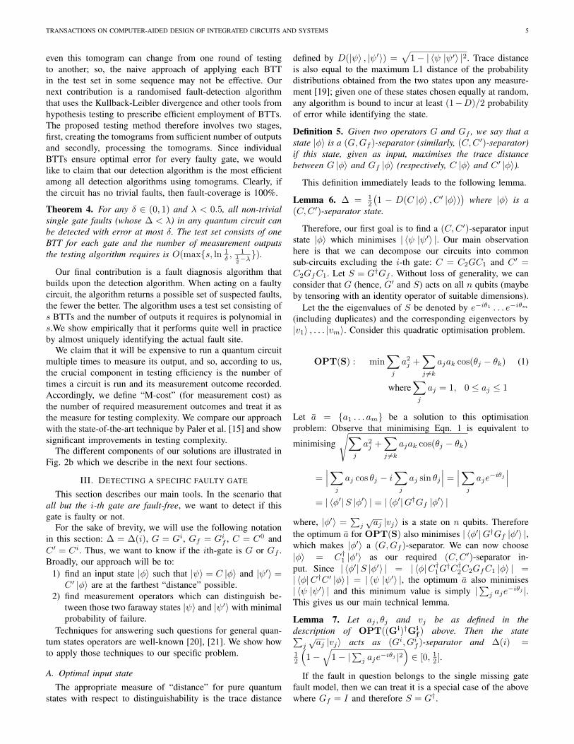
TRANSACTIONS ON COMPUTER-AIDED DESIGN OF INTEGRATED CIRCUITS AND SYSTEMS 5

even this tomogram can change from one round of testingto another; so, the naive approach of applying each BTTin the test set in some sequence may not be effective. Ournext contribution is a randomised fault-detection algorithmthat uses the Kullback-Leibler divergence and other tools fromhypothesis testing to prescribe efficient employment of BTTs.The proposed testing method therefore involves two stages,first, creating the tomograms from sufficient number of outputsand secondly, processing the tomograms. Since individualBTTs ensure optimal error for every faulty gate, we wouldlike to claim that our detection algorithm is the most efficientamong all detection algorithms using tomograms. Clearly, ifthe circuit has no trivial faults, then fault-coverage is 100%.

Theorem 4. For any δ ∈ (0, 1) and λ < 0.5, all non-trivialsingle gate faults (whose ∆ < λ) in any quantum circuit canbe detected with error at most δ. The test set consists of oneBTT for each gate and the number of measurement outputsthe testing algorithm requires is O(max{s, ln 1

δ ,1

12−λ}).

Our final contribution is a fault diagnosis algorithm thatbuilds upon the detection algorithm. When acting on a faultycircuit, the algorithm returns a possible set of suspected faults,the fewer the better. The algorithm uses a test set consisting ofs BTTs and the number of outputs it requires is polynomial ins.We show empirically that it performs quite well in practiceby almost uniquely identifying the actual fault site.

We claim that it will be expensive to run a quantum circuitmultiple times to measure its output, and so, according to us,the crucial component in testing efficiency is the number oftimes a circuit is run and its measurement outcome recorded.Accordingly, we define “M-cost” (for measurement cost) asthe number of required measurement outcomes and treat it asthe measure for testing complexity. We compare our approachwith the state-of-the-art technique by Paler et al. [15] and showsignificant improvements in testing complexity.

The different components of our solutions are illustrated inFig. 2b which we describe in the next four sections.

III. DETECTING A SPECIFIC FAULTY GATE

This section describes our main tools. In the scenario thatall but the i-th gate are fault-free, we want to detect if thisgate is faulty or not.

For the sake of brevity, we will use the following notationin this section: ∆ = ∆(i), G = Gi, Gf = Gif , C = C0 andC ′ = Ci. Thus, we want to know if the ith-gate is G or Gf .Broadly, our approach will be to:

1) find an input state |φ〉 such that |ψ〉 = C |φ〉 and |ψ′〉 =C ′ |φ〉 are at the farthest “distance” possible.

2) find measurement operators which can distinguish be-tween those two faraway states |ψ〉 and |ψ′〉 with minimalprobability of failure.

Techniques for answering such questions for general quan-tum states operators are well-known [20], [21]. We show howto apply those techniques to our specific problem.

A. Optimal input stateThe appropriate measure of “distance” for pure quantum

states with respect to distinguishability is the trace distance

defined by D(|ψ〉 , |ψ′〉) =√

1− | 〈ψ |ψ′〉 |2. Trace distanceis also equal to the maximum L1 distance of the probabilitydistributions obtained from the two states upon any measure-ment [19]; given one of these states chosen equally at random,any algorithm is bound to incur at least (1−D)/2 probabilityof error while identifying the state.

Definition 5. Given two operators G and Gf , we say that astate |φ〉 is a (G,Gf )-separator (similarly, (C,C ′)-separator)if this state, given as input, maximises the trace distancebetween G |φ〉 and Gf |φ〉 (respectively, C |φ〉 and C ′ |φ〉).

This definition immediately leads to the following lemma.

Lemma 6. ∆ = 12

(1 − D(C |φ〉 , C ′ |φ〉)

)where |φ〉 is a

(C,C ′)-separator state.

Therefore, our first goal is to find a (C,C ′)-separator inputstate |φ〉 which minimises | 〈ψ |ψ′〉 |. Our main observationhere is that we can decompose our circuits into commonsub-circuits excluding the i-th gate: C = C2GC1 and C ′ =C2GfC1. Let S = G†Gf . Without loss of generality, we canconsider that G (hence, G′ and S) acts on all n qubits (maybeby tensoring with an identity operator of suitable dimensions).

Let the the eigenvalues of S be denoted by e−iθ1 . . . e−iθm(including duplicates) and the corresponding eigenvectors by|v1〉 , . . . |vm〉. Consider this quadratic optimisation problem.

OPT(S) : min∑j

a2j +

∑j 6=k

ajak cos(θj − θk) (1)

where∑j

aj = 1, 0 ≤ aj ≤ 1

Let a = {a1 . . . am} be a solution to this optimisationproblem: Observe that minimising Eqn. 1 is equivalent to

minimising√∑

j

a2j +

∑j 6=k

ajak cos(θj − θk)

=∣∣∣∑j

aj cos θj − i∑j

aj sin θj

∣∣∣ =∣∣∣∑j

aje−iθj

∣∣∣= | 〈φ′|S |φ′〉 | = | 〈φ′|G†Gf |φ′〉 |

where, |φ′〉 =∑j

√aj |vj〉 is a state on n qubits. Therefore

the optimum a for OPT(S) also minimises | 〈φ′|G†Gf |φ′〉 |,which makes |φ′〉 a (G,Gf )-separator. We can now choose|φ〉 = C†1 |φ′〉 as our required (C,C ′)-separator in-put. Since | 〈φ′|S |φ′〉 | = | 〈φ|C†1G†C†2C2GfC1 |φ〉 | =| 〈φ|C†C ′ |φ〉 | = | 〈ψ |ψ′〉 |, the optimum a also minimises| 〈ψ |ψ′〉 | and this minimum value is simply |∑j aje

−iθj |.This gives us our main technical lemma.

Lemma 7. Let aj , θj and vj be as defined in thedescription of OPT((Gi)†Gi

f ) above. Then the state∑j

√aj |vj〉 acts as (Gi, Gif )-separator and ∆(i) =

12

(1−

√1− |∑j aje

−iθj |2)∈ [0, 1

2 ].

If the fault in question belongs to the single missing gatefault model, then we can treat it is a special case of the abovewhere Gf = I and therefore S = G†.

TRANSACTIONS ON COMPUTER-AIDED DESIGN OF INTEGRATED CIRCUITS AND SYSTEMS 6

If G acts on n′ qubits and n′ � n (say, n′ = 1 or 2), then itis possible to solve OPT(S) using the larger n-qubit operatorIn−n′⊗Gi. This may be computationally expensive, so a betteralternative is to let S = G†Gf as before, and let T = In−n′⊗Sbe the extension of S to n qubits. If {(e−iθj , |vj〉)} are theeigen-pairs of S then it is easy to see that {(e−iθj , |vj〉 ⊗|0〉⊗n−n

′)} are the eigen-pairs of T . Thus our required input

state can be derived as |φ〉 = C†1(|φ′〉 ⊗ |0〉⊗(n−n′) ) where

|φ′〉 is a (G,Gf )-separator input state. For example, if G isa single qubit gate, then we only need to store that |φ′〉 is1√2

(|v1〉+ |v2〉) where |v1〉 and |v2〉 are the eigenvectors ofG†Gf , irrespective of the value of n.

It should be obvious that our method of decomposing acircuit into portions before and after the gate in question canalso be used for multiple missing/defective gate faults as longas the faulty gates can be grouped together and the circuit canbe sliced around them. For example, our method is applicableto multiple gate faults if they act on distinct set of qubits,and/or are adjacent to each other; trivial extension is requiredto the computation of optimal state described earlier.

We end this subsection with a proof of Lemma 2 whichcharacterises faults with ∆ = 0.5 as the trivial faults.

Proof of Lemma 2. Consider a trivial fault, i.e., Gf = eiαGfor some G acting on w qubits. Then, S = eiαI and this hasone eigenvalue eiα with multiplicity m = 2w. The solution ofthe optimisation problem can be readily seen to be ai = 1

m .This gives us ∆ = 0.5 which implies an untestable fault.

For the other direction, consider some gate G and itsuntestable faulty version Gf . Therefore, ∆ = 0.5 whichimplies that |∑j aje

−iθj |2 = 1. Suppose that at least twoof θj’s are distinct. It is easy to verify that any convexcombination of such a set of points on the unit circle in thecomplex plane has modulus less than 1. Therefore, all theθj must be equal. Since S is diagonalisable (it is unitary),G†Gf = S = V · e−iθjI · V −1 for some V . Therefore, G†Gfis same as e−iθjI which implies that Gf = e−iθjG, i.e., thefault simply changes the global phase of G.

B. Optimal measurement operators

Once we have obtained the optimal input state |φ〉, wecan compute the two possible output states |ψ〉 = C |φ〉and |ψ′〉 = C ′ |φ〉. Quantum states are manifested only bytheir measurement outputs. It is thus important to design andimplement measurement operators that are able to distinguishbetween |ψ〉 and |ψ′〉, and thereby determine if the circuitin question is C or C ′. However, unlike input states, mea-surement operators depend on the actual circuit and has to becomputed once for every circuit and every fault model.

The question of distinguishing between two given quantumstates is one of the classical problems of quantum computing[22]. Two states can be differentiated (using measurements)with certainty if and only if they are orthogonal. So, if Gf isalmost same as G, then obviously no measurement should beable to distinguish between them with high confidence.

There are two known modes of distinguishing between apair of states. Helstrom measurement is a two-output (von

|ψ′〉

|ψ〉|ω+〉

|ω−〉

keiκ

∆

∆

Fig. 3. Schematic diagram for the Helstrom projective measurement basis.The angles represent the inner product between the corresponding statevectors.

Neumann) projective measurement which minimises the errorof incorrect labelling [20]. If we prohibit incorrect outcomeand instead allow our measurement operators to either label astate with certainty or report “§”(inconclusive), then we wouldbe performing unambiguous state discrimination (USD) [23]–[25]. We will use Helstrom projective measurement in the restof this paper for explaining our technique; however, we couldhave also used USD for doing the same.

The concept behind Helstrom projective measurement isexplained in Figure 3. Our derivation follows similar approachas in [20], [21] but is in a form that suits our problem.

First we create an orthonormal basis |ω+〉 and |ω−〉 whichspans |ψ〉 and |ψ′〉. This basis will be used for measurementand we will infer the state as |ψ〉 or |ψ′〉 upon measurementoutcome |ω+〉 or |ω−〉, respectively. We want to minimisethe probability of error (when state is |ψ〉 but outcome isincorrectly |ω−〉 and similarly for the other pair); so the basisstates should be maximally away from the output states, i.e.,| 〈ω− |ψ〉 |2 = | 〈ω+ |ψ′〉 |2.

We will represent by keiκ the complex number 〈ψ |ψ′〉 =∑j aje

−iθj in which aj’s are the solution of OPT(S) andeiθj are the eigenvalues of S = G†Gf .

We first represent our states in terms of our basis states,i.e., |ψ〉 = α1 |ω+〉+ β1 |ω−〉 and |ψ′〉 = α2 |ω+〉+ β2 |ω−〉.Without loss of generality, we can take α1 as a real numberr1. The condition of equal probability of error enforces theserepresentations: β1 = r2e

ix1 for some real r2 =√

1− r21 ,

α2 = r2eix2 and β2 = r1e

ix3 . Equating keiκ = 〈ψ |ψ′〉 =r1r2e

ix2(1 + ei(x3−x1−x2)), we obtain one possible solution:x1 = 0, x2 = κ, x3 = κ and r1,2 =

(√1 + k ±

√1− k

)/2

which produces this basis:

|ω+〉 =−r1

r22 − r2

1

|ψ〉+r2e−iκ

r22 − r2

1

|ψ′〉

|ω−〉 =r2

r22 − r2

1

|ψ〉 − r1e−iκ

r22 − r2

1

|ψ′〉

Therefore, we obtain the three following projectors todistinguish between |ψ〉 and |ψ′〉: {P0 = |ω+〉 〈ω+| , P1 =|ω−〉 〈ω−| , P§ = I − P0 − P1} with outcomes 0, 1 and §,respectively. The outcome 0 corresponds to the output statebeing |ψ〉 and hence implies that the circuit is (probably) fault-free; similarly, outcome 1 implies that the i-th gate is probablyfaulty. Outcome § is never observed if circuit is fault-free orif the i-th gate is faulty; therefore, outcome § immediatelysignifies that the circuit has fault at some other gate.

TRANSACTIONS ON COMPUTER-AIDED DESIGN OF INTEGRATED CIRCUITS AND SYSTEMS 7

C. Optimal BTT

Without loss of generality, we will henceforth assume thatall our faults are non-trivial, i.e., ∆ < 0.5.

Definition 8. Binary tomographic test for the i-th missinggate, denoted by BTT (i), is defined as the combination ofa (C0, Ci)-separator input and corresponding measurementoperator {P0, P1, P§}.

We capture the result of application of any BTT on anycircuit C by the probability distribution on the measurementoutcomes.

Definition 9. µi,j is defined as the probability distribution{p(0), p(1), p(§)} of measurement outcomes when BTT (i) isemployed on circuit Cj .

The probability of error after one measurement wouldbe at most | 〈ψ |ω−〉 |2 = r2

2 =(1−√

1− k2)/2 =(

1−√

1− |∑j aje−iθj |2

)/2 which matches the minimum

probability of error in distinguishing |ψ〉 and |ψ′〉 by anyprojective measurement. This establishes the following lemmaon the optimality of a BTTs error.

Lemma 10. The output distribution of BTT (i) on the fault-free circuit C0 is µi0 = {1−∆(i),∆(i), 0} and the distribu-tion on the faulty circuit Ci is µii = {∆(i), 1−∆(i), 0}.Discussion of Theorem 3. Lemma 10 shows that BTT (i) canoptimally distinguish between a fault-free gate and a faultygate, as long as it is a non-trivial fault.

The computationally significant steps are that of determin-ing the (G,Gf )-separator and calculating the input state to thecircuit and the optimal measurement operator.

The latter involves (a) determining the input state |φ〉 to thecircuit from the (G,Gf )-separator |φ′〉 (b) determining theoutput states |ψ〉 and |ψ′〉 of the fault-free and faulty circuitsfrom the input state, and (c) determining the measurementoperator {P0, P1, P§} on the output states. Many efficient pro-gramming platforms and libraries exist today to numericallycalculate these states and operators.

The former step involves solving the quadratic program (1)on 2w variables, where w is the number of qubits of thei-th gate. Quadratic programming is in general an NP-hardproblem, but we believe its use in deriving the BTT is not acomputational hurdle for a couple of reasons. First, the numberof variables is exponential only in the dimension of the gateinvolved, which is usually quite small in literature we haveencountered so far; also, it is also likely that synthesis ofgates acting of many qubits is going to be difficult. Secondly,observe the interesting fact that the separator input for a gatein a circuit depends fundamentally on the gate in questionand corresponding fault model. It does not depend at all onthe portion of the circuit coming after the faulty gate, andits dependence on the portion of the circuit before the faultygate is really incidental. Therefore, it is feasible to have apre-computed table of (G,Gf )-separators for different gatesunder common fault models. The required separator input forany circuit can be obtained by running the first portion of thecircuit in reverse on a gate-separator input. Thus, the major

H

H

Ry(π/6

)

|q3〉

|q1〉

|q2〉

Rz(π/1

6)

Fig. 4. Benchmark circuit 3qubit-CNOT on 3 qubits with 6 gates. The 2-qubitrotation gates apply the rotation operations to both the qubits.

computation tasks of eigen-decomposition of S and solvingOPT(S) can be done only once and reused as needed.

Table I shows the probability of error in detecting SMGFfaults for some of the commonly used quantum gates. Thetable demonstrates that (a) for most gates (for example,Hadamard), missing gate faults can be easily detected with cer-tainty, and (b) there are some gates (for example, Rz(π/212))for which SMGF will be quite hard to detect.

IV. TEST GENERATION

Algorithm 1 Test generation stageInput: C0 = 〈G1 . . . Gs〉: Fault-free gates

{G1f , . . . G

sf}: Faulty gates

Output: T : BTT table∆: Fault error table

1: Initialise empty s× (1 + s) table T and s× 1 table ∆2: for i = 1 to s do3: Break C0 into C1 and C2 around i-th gate4: Compute Ci from C0 and Gif5: {(e−iθ1 , |v1〉), . . . (e−iθm , |vm〉)} ← eigen-

decomposition of (Gi)†Gif6: ~a← solution of OPT((Gi)†Gi

f )7: Compute ∆[i]← |∑j aje

−iθj |8: Compute |φ′〉 =

∑j

√aj |vj〉 and |φ〉 = C†1 |φ′〉

9: Compute |ψ〉 = C0 |φ〉, |ψ′〉 = Ci |φ〉10: Compute |ω+〉 and |ω−〉11: Compute P0, P1, P§12: for j = 0 to s do13: Compute |α〉 = Cj |φ〉14: Compute pk = 〈α |Pk|α〉, for k = 0, 1, §15: T [i, j]← (p0, p1, p§)16: end for17: end for18: return T,∆

In this section we use the BTT s defined in Section IIIto generate a test-set that, for us, consists of BTT-table anda fault-error table. The BTT-table is a generalisation ofthe fault-table constructed by Aligala et al. [16]; for eachBTT , it contains the corresponding probability distributionon outcomes.

The test generation stage (illustrated in Algorithm 1) takesas input a description of the circuit, along with each ofthe fault-free and faulty operators. First, for each gate Gi,we construct the input state and measurement operator forBTT (i). Then, we construct a BTT table with s rows and

TRANSACTIONS ON COMPUTER-AIDED DESIGN OF INTEGRATED CIRCUITS AND SYSTEMS 8

TABLE IMINIMUM PROBABILITY OF ERROR (∆) FOR DETECTING (SINGLE) MISSING GATE. THE GATES IN THE CLIFFORD+T SET OF QUANTUM GATES ARE

MARKED IN bold – THIS SET IS GAINING POPULARITY FOR CONSTRUCTING FAULT-TOLERANT QUANTUM CIRCUITS.

Gate Error prob. Gate Error prob. Gate Error prob. Gate Error prob. Gate Error prob. Gate Error prob.

Hadamard 0.00 Pauli-Z 0.00 CNOT 0.00 Phase = Rz(π2

) 0.15 Rz(π/16) 0.415 Rz(π/28) 0.495Pauli-X 0.00 Pauli-Y 0.00 Toffoli 0.00 T = Rz(π/4) 0.31 Rz(π/32) 0.458 Rz(π/212) 0.4997

(1 + s) columns whose (q, r)-th cell contains the distributionµq,r when BTT (q) is applied to circuit Cr and a fault-errorarray whose r-th entry ∆(r) contains the minimum possibleprobability of error in distinguishing between C0 and Cr.

BTT table and fault-error array for a benchmark circuit3qubitcnot (illustrated in Figure 4) are given in the Table II. Itcan be readily inferred by comparing the C0 and C5 columnsthat detecting missing G5 gate is more error-prone and is goingto require lots of samples.

Next we describe some important properties of the test-setthat are used by upcoming detection and diagnosis algorithms.

A. Test-set properties

If ∆(r) is close to 0.5, then C0 is almost similar to Cr andthen there is a large chance of error in distinguishing betweenC0 and Cr (it becomes impossible when ∆ = 0.5). So,we use a subroutine CleanupBTTTable(λ) which takesa user-parameter λ ∈ (0, 0.5) and ignores all faults witherror more than ∆. It does so by removing the (1 + r)-thcolumn (corresponding to Cr) and r-th row (corresponding toBTT (r)) from the BTT table.

Suppose, we apply a BTT on a circuit several times andrecord the distribution of outcomes. We use τ(i, C,m) todenote this distribution obtained by applying BTT (i) on C ∈{C0, . . . , Cs} m number of times. After sufficient numberof times of applying the test, the distribution is expected toconverge towards µi,j . But more importantly, for any i, mand Cj , τ(i, 0,m) = (a1, a2, 0) and τ(i, i,m) = (a3, a4, 0)for some a1, a2, a3, a4. So, in essence, we need to choosea large enough m such that a sampled distribution τ can beconfidently attributed to come from either µi,0 or µi,i. We willuse the Kullback-Leibler divergence, denoting it by DKL, fortesting closeness of τ with the source distributions. The nextlemma states the minimum number of samples needed.

Lemma 11. Choose any δ ∈ (0, 1) and some i ∈{1, . . . s} such that ∆(i) 6= 0.5. If m is selected as⌈

ln(1/δ)

− ln(2√

∆(i)(1−∆(i)))

⌉, then the following events have a prob-

ability at most δ.(a) DKL(τ‖µi,i) < DKL(τ‖µi,0) where τ is the distribution

of m samples drawn from µi,0.(b) DKL(τ‖µi,i) > DKL(τ‖µi,0) where τ is the distribution

of m samples drawn from µi,i.

Proof. We will give the proof for part (a). Part (b) can beproved similarly.

Let p denote 1 −∆(i). Note that for any i, µi,0 = (p, 1 −p, 0) and µi,i = (1 − p, p, 0). Since τ is obtained from µi,0,τ(§) = 0 and τ(0) can be written as x/m where x followsthe distribution Binomial(m, p).

Pr[DKL(τ‖µi,i) < DKL(τ‖µi,0)]

= Pr

∑z∈{0,1,§}

τ(z)lgµi,0(z)

lgµi,i(z)< 0

= Pr

[(m− 2x) lg

p

1− p > 0

]= Pr[x < m/2] since, p > 0.5

≤ exp

(−mDKL

((0.5, 0.5)‖(1− p, p)

))= exp

(m[1 +

1

2ln p(1− p)]

)The last inequality is an application of the Chernoff-Hoeffdingbound. The required bound on m follows immediately bysetting the final expression to δ.

We use η(i, δ) (or ηi in short when δ is fixed) to denotethe above bound m on the number of samples required forBTT (i) for a particular δ. The subroutine NumSamples()computes ηi for all i = 1 . . . s.

Let ηmax denote the maximum sample size and ηavg denote∑si=1 ηi/s. We now upper bound all these values.

Lemma 12. Suppose for some i, ∆(i) ≤ λ for some λ ≤ 1/2.

Then, {ηi, ηmax, ηavg} ≤ln(1/δ)

2(

12 − λ

)2 + 1.

TABLE IIBTT-TABLE AND FAULT-ERROR ARRAY FOR CIRCUIT 3QUBITCNOT WITH SINGLE MISSING GATE FAULTS

Test C0 C1 C2 C3 C4 C5 C6

BTT(1) (1.00,0.00,0.00) (0.00,1.00,0.00) (0.28,0.09,0.63) (0.30,0.50,0.20) (0.92,0.04,0.05) (0.99,0.00,0.01) (0.91,0.00,0.09)BTT(2) (1.00,0.00,0.00) (0.02,0.13,0.85) (0.00,1.00,0.00) (0.50,0.00,0.50) (0.87,0.00,0.13) (0.99,0.00,0.01) (0.76,0.00,0.24)BTT(3) (1.00,0.00,0.00) (0.73,0.13,0.15) (0.50,0.00,0.50) (0.00,1.00,0.00) (0.87,0.06,0.07) (0.98,0.00,0.02) (0.86,0.00,0.14)BTT(4) (0.75,0.25,0.00) (0.75,0.25,0.00) (0.38,0.13,0.50) (0.00,0.00,1.00) (0.25,0.75,0.00) (0.74,0.24,0.02) (0.19,0.07,0.74)BTT(5) (0.60,0.40,0.00) (0.29,0.20,0.52) (0.20,0.30,0.50) (0.55,0.38,0.07) (0.52,0.35,0.13) (0.40,0.60,0.00) (0.25,0.25,0.50)BTT(6) (1.00,0.00,0.00) (0.33,0.29,0.38) (0.06,0.22,0.72) (0.10,0.42,0.48) (0.87,0.02,0.11) (0.99,0.01,0.00) (0.00,1.00,0.00)∆ N.A. 0 0 0 0.25 0.4 0

TRANSACTIONS ON COMPUTER-AIDED DESIGN OF INTEGRATED CIRCUITS AND SYSTEMS 9

Proof. It suffices to lower bound − ln(2√

∆(i)(1−∆(i))) by2( 1

2 − λ)2. This is done as follows.

− ln(2√

∆(i)(1−∆(i)))

≥ − ln(2√λ(1− λ))

(since, ∆(1−∆) is increasing in [0, 0.5])

= − ln 2− 1

2lnλ− 1

2ln(1− λ)

= −1

2[ln(1 + 2ε) + ln(1− 2ε)] (let ε = 1

2 − λ)

≥ −1

2

[−2

(2ε)2

2− 2

(2ε)4

4− . . .

]≥ 2ε2 = 2(

1

2− λ)2

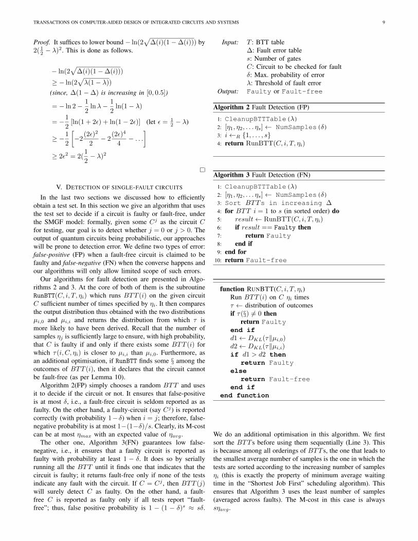
V. DETECTION OF SINGLE-FAULT CIRCUITS

In the last two sections we discussed how to efficientlyobtain a test set. In this section we give an algorithm that usesthe test set to decide if a circuit is faulty or fault-free, underthe SMGF model: formally, given some Cj as the circuit Cfor testing, our goal is to detect whether j = 0 or j > 0. Theoutput of quantum circuits being probabilistic, our approacheswill be prone to detection error. We define two types of error:false-positive (FP) when a fault-free circuit is claimed to befaulty and false-negative (FN) when the converse happens andour algorithms will only allow limited scope of such errors.

Our algorithms for fault detection are presented in Algo-rithms 2 and 3. At the core of both of them is the subroutineRunBTT(C, i, T, ηi) which runs BTT (i) on the given circuitC sufficient number of times specified by ηi. It then comparesthe output distribution thus obtained with the two distributionsµi,0 and µi,i and returns the distribution from which τ ismore likely to have been derived. Recall that the number ofsamples ηj is sufficiently large to ensure, with high probability,that C is faulty if and only if there exists some BTT (i) forwhich τ(i, C, ηi) is closer to µi,i than µi,0. Furthermore, asan additional optimisation, if RunBTT finds some § among theoutcomes of BTT (i), then it declares that the circuit cannotbe fault-free (as per Lemma 10).

Algorithm 2(FP) simply chooses a random BTT and usesit to decide if the circuit or not. It ensures that false-positiveis at most δ, i.e., a fault-free circuit is seldom reported as asfaulty. On the other hand, a faulty-circuit (say Cj) is reportedcorrectly (with probability 1− δ) when i = j; therefore, false-negative probability is at most 1−(1−δ)/s. Clearly, its M-costcan be at most ηmax with an expected value of ηavg .

The other one, Algorithm 3(FN) guarantees low false-negative, i.e., it ensures that a faulty circuit is reported asfaulty with probability at least 1 − δ. It does so by seriallyrunning all the BTT until it finds one that indicates that thecircuit is faulty; it returns fault-free only if none of the testsindicate any fault with the circuit. If C = Cj , then BTT (j)will surely detect C as faulty. On the other hand, a fault-free C is reported as faulty only if all tests report “fault-free”; thus, false positive probability is 1 − (1 − δ)s ≈ sδ.

Input: T : BTT table∆: Fault error tables: Number of gatesC: Circuit to be checked for faultδ: Max. probability of errorλ: Threshold of fault error

Output: Faulty or Fault-free

Algorithm 2 Fault Detection (FP)

1: CleanupBTTTable(λ)2: [η1, η2, . . . ηs]← NumSamples(δ)3: i←R {1, . . . , s}4: return RunBTT(C, i, T, ηi)

Algorithm 3 Fault Detection (FN)

1: CleanupBTTTable(λ)2: [η1, η2, . . . ηs]← NumSamples(δ)3: Sort BTTs in increasing ∆4: for BTT i = 1 to s (in sorted order) do5: result← RunBTT(C, i, T, ηi)6: if result == Faulty then7: return Faulty8: end if9: end for

10: return Fault-free

function RUNBTT(C, i, T, ηi)Run BTT (i) on C ηi timesτ ← distribution of outcomesif τ(§) 6= 0 then

return Faultyend ifd1← DKL(τ‖µi,0)d2← DKL(τ‖µi,i)if d1 > d2 then

return Faultyelse

return Fault-freeend if

end function

We do an additional optimisation in this algorithm. We firstsort the BTT s before using them sequentially (Line 3). Thisis because among all orderings of BTT s, the one that leads tothe smallest average number of samples is the one in which thetests are sorted according to the increasing number of samplesηi (this is exactly the property of minimum average waitingtime in the “Shortest Job First” scheduling algorithm). Thisensures that Algorithm 3 uses the least number of samples(averaged across faults). The M-cost in this case is alwayssηavg .

TRANSACTIONS ON COMPUTER-AIDED DESIGN OF INTEGRATED CIRCUITS AND SYSTEMS 10

Proof of Theorem 4. Both Algorithms 2(FP) and 3(FN) usea test set consisting of s BTTs and can detect all non-trivial faults with ∆ < λ. Algorithm 2(FP) ensures that theprobability of false-positive is at most δ and Algorithm 3(FN)ensures that the false-negative probability is at most δ. Thenumber of circuit outputs required by the former algorithm isat most 1 + ln(1/δ)/2(0.5 − λ)2 and the same by the latteralgorithm is at most s(1 + ln(1/δ)/2(0.5− λ)2).

VI. DIAGNOSIS OF SINGLE-FAULT CIRCUITS

In this section we discuss our solution for fault diagnosis —not only we are interested in finding out if a given quantumcircuit has a (single gate) fault, but we want to identifythe particular fault as well. As in Section V, our diagnosticstrategy uses the BTT-table and the fault-error table generatedby the test generation stage (Algorithm 1).

Our algorithm is described in Algorithm 4. It first generatessome candidate faults (denoted by CAND), and then verifiesif each candidate can be the possible fault by comparing theobtained distribution with the possible distribution. Describedin lines 8–17 and similar to the algorithm for detection,CAND is obtained by first removing all i for which BTT (i)has non-zero § outcomes. The faults left behind are furtherfiltered using KL-Divergence. For any i for which τi[§] = 0,we accept i as a candidate if the obtained distribution τ iscloser to µi,i than µi,0. We wanted to ensure two propertiesof CAND — (i) if C = Cj , then j should be in CAND (nofalse negative), and (ii) if C = Cj , the CAND should notcontain any i 6= j (no false positives).

However, the above steps are insufficient in removing falsepositives, so we propose two additional heuristics to reducefalse positives and also ensure no false negative. In thosetwo heuristics (lines 18–24 and lines 25–35, respectively),the set of candidates are further pruned based on additionalproperties of the entire list of distributions [τ1, τ2, . . . τs] usingtwo additional tables Map1 and Map2, created by subroutinesCreateMap1 and CreateMap2, respectively. For everyfaulty circuit Cj , i ∈ Map1[j] if BTT (i), when appliedon Cj , would never output §. On the other hand, Map2[j]contains those BTTs whose majority outcome would be 0.

Similar to the earlier algorithm for fault detection, thisalgorithm also choose the number of samples carefullyto ensure bounded error during diagnosis. The subroutineNumSampleDiag() essentially sets ηi to be max(ηai , η

bi , η

ci )

(see Algorithm 4) where these have the following properties.• ηai = η(i, δ) is defined in Lemma 11,• ηbi is a large enough integer such that if for any j,µi,j [§] > 0, then ηbi samples from µi,j will contain non-zero § with probability at least 1− δ (see Lemma 13),

• ηci is a large enough integer such that if any µi,j [0] > 0.5,then ηci samples from µi,j will have 0 as the majoritysample with probability at least 1− δ (see Lemma 14).

Lemma 13. Suppose for some i and j, µi,j(§) 6= 0. Let τidenote a distribution obtained from ηbi,j independently chosensamples from µi,j . Then Prτi [τi(§) = 0] ≤ δ. Here, ηbi,j =

lg(δ)lg(1−µi,j(§)) if µi,j(§) 6= 1 and 1 otherwise.

The proof of the above lemma is straight-forward andomitted. We set ηbi = maxj η

bi,j .

Lemma 14. Suppose for some i and j, µi,j(0) > 1/2. Let τidenote a distribution obtained from ηci,j independently chosensamples from µi,j where ηci,j = 2µi,j(0) ln(1/δ)

(µi,j(0)−1/2)2 . ThenPrτi [τi(0) ≤ 1/2] ≤ δ.

This lemma can be proved using Chernoff bound 3. We setηci = maxj η

ci,j .

Since ηi is set to max{ηai , ηbi , ηci }, we can say that thesample size for BTT (i) ensures that Lemma 11, 13 and 14are satisfied. We denote ηmax = maxi ηi and ηavg =

∑i ηi/s.

It is clear that Algorithm 4 always uses∑i ηi samples. We

prove its correctness next.

Theorem 15. Suppose C = Cj for some j > 0.(a) Then, SUSP returned by Algorithm 4 contains j with

probability at least 1− 2δ.(b) Consider any 0 < i 6= j. Then, SUSP returned by

Algorithm 4 does not contain i with probability at least 1− δunless µi,j = (p, 1− p, 0) for some p ≤ 1/2.

Furthermore, M-cost of Algorithm 4 is s · ηavg .

Proof of part(a). We will essentially prove three claims;j ∈ CAND, j 6∈ REJ1 and j 6∈ REJ2, each holding withhigh probability.

Since µj,j(§) = 0, therefore, τj(§) = 0 when BTT (j) isapplied. Lemma 11 gives us that Pr[j added to CAND] ≥1− δ (lines 11–15).

By the property of Map1, for any i ∈Map1[j], τi(§) = 0since τi is obtained by running BTT (i) on Cj . Therefore, jwill not be added to REJ1 (in line 21).

Finally, we show j 6∈ REJ2 w.h.p. by using a probabilisticreasoning. For all k ∈ {1, . . . , s}, let Xk denote the followingindicator random variable.

Xk =

{1, if k ∈Map2[j] & τk(0) < 1/20, otherwise

}First, note that

∑kXk is precisely the value of count before

line 32. Secondly, Pr[Xk] < δ since (a) if µk,j(0) ≤1/2, k 6∈ Map2[j], and (b) if µk,j(0) > 1/2, thenPr[τk(0) ≤ 1/2] < δ (by Lemma 14). Therefore, E[count] =∑k E[Xk] < sδ. We apply Chernoff bound 4 to upper

bound Pr[j added to REJ2] = Pr[count ≥ sδ(1 + t)] ≤exp(− t2

2+tsδ).Case (a) sδ ≤ 1: In this case, t = 2

sδ ln 1δ and so, 2t > 2+t.

Therefore, exp(− t2

2+tsδ) ≤ exp(− t2sδ) ≤ δ.

Case (b) sδ > 1: Note that in this case, if t > s, then(1 + t)sδ > s2δ > s; however, count can never be more thans. Therefore, we can take t ≤ s and so, 2+ t < 2s. Therefore,exp(− t2

2+tsδ) ≤ exp(− t2

2ssδ) = exp(− t2δ2 ) which is at most

δ since t =√

2δ ln 1

δ in this case.

3We use the following application of Chernoff bound. Let X denote thenumber of heads when n coins are tossed, each with probability of head equalto p > 1/2. Then, Pr[X > n/2] ≥ 1− exp(− n

2p(p− 1

2)2).

4We are using the following version: For any σ > 0, Pr[∑Xk ≥ (1 +

σ)E] ≤ exp(− σ2

2+σE) where E is E[Xk] or any upper bound on it [26].

TRANSACTIONS ON COMPUTER-AIDED DESIGN OF INTEGRATED CIRCUITS AND SYSTEMS 11

Input: T : BTT table∆: Fault error tables: Number of gatesC: Circuit to be checked for faultδ: Max. probability of errorλ: Threshold of fault error

Output: Faulty or Fault-free

Algorithm 4 Fault Diagnosis

1: CleanupBTTTable(λ)2: For i = 1 to s, ηi ← NumSampleDiag(δ, i)3: For j = 1 to s, Map1[j]← CreateMap1(δ, j)4: For j = 1 to s, Map2[j]← CreateMap2(δ, j)5: Initialise CAND ← {}, REJ1← {}, REJ2← {}6: if sδ ≤ 1, t←

√2δ ln 1

δ else t← 2sδ ln 1

δ

7: for BTT i = 1 to s do8: Run BTT (i) on C ηi times9: τi ← distribution of outcomes

10: if τi(§) = 0 then11: d0← DKL(τi‖µi,0)12: d1← DKL(τi‖µi,i)13: if d0 > d1 then14: Add i to CAND15: end if16: end if17: end for18: for j in CAND do19: for i in Map1[j] do20: if τi[§] 6= 0 then21: Add j to REJ1; break;22: end if23: end for24: end for25: for j in CAND do26: count← 027: for k in Map2[j] do28: if τk[0] < 1/2 then29: count← count+ 130: end if31: end for32: if count ≥ sδ(1 + t) then33: Add j to REJ234: end if35: end for36: SUSP ← CAND \REJ2 \REJ137: return SUSP

function NUMSAMPLEDIAG(δ, i)d0← µi,0d1← µi,iif d0 = (1, 0, 0) or (0, 1, 0) then

ηai ← 1else

ηai ← η(i, δ) (Lemma 11)end ifηai ← 1, ηci ← 1for BTT j = 1 to s s.t. do

if 0 < µi,j(§) < 1 thenηbi ← max

{ηbi ,

log(δ)log(1−µi,j(§))

}end ifif µi,j(0) > 1/2 then

ηci ← max{ηci ,

2µi,j(0) ln(1/δ)(µi,j(0)−1/2)2

}end if

end forreturn max{ηai , ηbi , ηci }

end function

function CREATEMAP1(δ, j)Initialise Map1[j] = {}for faulty circuit i = 1 . . . s do

if µi,j(§) = 0 thenAdd i to Map1[j]

end ifend forreturn Map1[j]

end function

function CREATEMAP2(δ, j)Initialise Map2[j] = {}for faulty circuit k = 1 . . . s do

if µk,j(0) > 1/2 thenAdd k to Map2[j]

end ifend forreturn Map2[j]

end function

TRANSACTIONS ON COMPUTER-AIDED DESIGN OF INTEGRATED CIRCUITS AND SYSTEMS 12

Therefore, j is added to REJ2 with probability at most δ.Combining all the scenarios, j is not in SUSP either if j isnot added to CAND or j is also added to REJ2 – whichhappens with probability at most 2δ.

We need the following results on the sample sizes to provethat false positives happen with low probability.

Lemma 16. Let τi be a distribution obtained from ηi runsof BTT (i) on a circuit Cj for some i 6= j. If µi,j [§] = 0,µi,0[0] < 1 and µi,j [0] > 1/2, then with probability at least1− δ, DKL(τ‖µi,0) ≤ DKL(τ‖µi,i) holds.

Proof. Let a = τ [0] and p = µi,0[0] (note that 1/2 < p < 1).Therefore, µi,0 = (p, 1− p, 0) and µi,i = (1− p, p, 0).

DKL(τ‖µi,0)−DKL(τ‖µi,i)

= a lga

p+ (1− a) lg

1− a1− p − a lg

a

1− p − (1− a) lg1− ap

= a lg1− pp

+ (1− a) lgp

1− p= (1− 2a) lg

p

1− p> 0 iff a < 1/2

Now we are ready to give a bound on the false positive.Please observe that, unlike the bounds given until now, thisbound does not hold for all scenarios. In fact, if µi,j is similarto µi,i (i.e., both have the form (p, 1−0, 0) for some p < 1/2),then we allow i to be erroneously included in CAND. Wedo this to keep our tests simple and hope that the additionalheuristics of Map1 and Map2 will ensure that such i iseliminated from SUSP . We will demonstrate the effectivenessof these heuristics with the help of our experiment results.

Proof of Theorem 15(b). Let τi be the distribution obtainedfrom µi,j . We will separately analyse two possible scenarios.

First possibility is that µi,j(§) > 0. Then, τi(§) 6= 0 withprobability at least 1 − δ using Lemma 13. Therefore, withhigh probability, i will not be added to CAND (lines 11–15).

The other possibility is that µi,j = (p, 1 − p, 0) for somep > 1/2 leading to τi = (r, 1 − r, 0) for some r. Now,let µi,0 = (q, 1 − q, 0) for some q > 1/2. (a) If q = 1,then µi,i = (0, 1, 0). By Lemma 14, Pr[r > 1/2] ≥ 1 − δ.Therefore, with high probability of 1 − δ, τi 6= (0, 1, 0) andin that case, i will not be added to CAND in lines 11–15since DKL(τi‖µi,i) is not even defined for such µi,i and τi.(b) On the other hand, if q < 1, then d0 and d1 in lines 11–15 are well-defined. But DKL(τ‖µi,0) ≤ DKL(τ‖µi,i) withhigh probability (Lemma 16) and in that case, i is not addedto CAND in those lines.

VII. PERFORMANCE EVALUATION

The primary objective of our work was to derive theoret-ical upper bounds for detecting and diagnosing every non-redundant fault with high probability.

However, we also evaluated our approach for practicalscenarios by running simulations to compare our algorithm

|q0〉

H3

•H2 X2

•X2

H3|q1〉 • H ⊕ H

|q2〉 ⊕

Fig. 5. Benchmark circuit simpleGrover on 3 qubits with 9 gates

with the state-of-the-art algorithm by Paler et al. [15]. We usedthe SMGF model for faults in our experiments, i.e., the faultygate is assumed to be missing. Due to the obvious difficultyof not having access to an affordable quantum computer, wesimulated a run of BTT , say BTT (i) on circuit Cj , bysampling from the distribution µi,j in the BTT table. Forevery circuit and every fault, we ran fault detection algorithms10,000 times and report their mean. For our experiments, wefixed the probability of error (δ) at 1%, same as that in thework we are comparing with. We set λ = 0.499995, so everyfault was within the threshold for detection. All our programs,written in python, as well as fault-error and BTT tables forour benchmark circuits are available on our website 5.

The benchmark circuits that we used are 3qubitcnot (il-lustrated in Figure 4), simpleGrover3 (implementation ofGrover’s algorithm on 3 qubits and illustrated in Figure 5)and qecc9 (part of QuIDDPro software package [27]). Wecould not obtain exactly same circuits for qftadd5 and qftadd12that were used in the compared work, so we include resultsof our experiments but leave out corresponding results fromthe previous work. In Table III we have listed their relevantproperties along with a histogram of how many faulty gateshave error (∆(G,Gf )) in different intervals. The gates with∆ ≈ 0 are very easy to detect, if faulty. On the other hand, thegates with ∆ ≈ 0.5 would be impossible to detect when faultyand such faults are called as redundant faults. However, it canbe observed that none of the single missing gate faults in ourbenchmark circuits were redundant and moreover, most gatesin 3qubitcnot, simpleGrover3 and qecc9 appear to be easilydetectable. In contrast, qftadd5 and qftadd12 contains severalgates with high ∆; so, it is expected that those circuits willincur a high M-cost for detection and diagnosis.

A. Results for detection

For comparison, we choose the BTT gen algorithm alongwith the LRM technique (denoted by BTT+LRM) proposed byPaler et al. [15] which is currently the best fault detection algo-rithm (it substantially improves upon their earlier work [14]).Even though they were only concerned with false-negatives,we report M-costs for both types of errors.

We chose to implement “Algorithm FN” since the BTT genalgorithm was evaluated only for faulty circuits. Since mostfaults in the benchmark circuits have low ∆, their corre-sponding η is quite small. We observed that for such circuits,ηmax ≈ sηavg (also reported in Table III), so Algorithm FNshould be able to detect most of their faults using few samples.

Detailed performance of our algorithm for all 7 types offaults (including “fault-free”) for the 6 gates of the 3qubitcnot

5https://www.iiitd.edu.in/∼dbera/smgf/

TRANSACTIONS ON COMPUTER-AIDED DESIGN OF INTEGRATED CIRCUITS AND SYSTEMS 13

TABLE IIIBENCHMARK CIRCUITS

Benchmarkcircuit

qubits gates faults with∆ = 0

faults with 0 <∆ ≤ 0.05

faults with 0.05 <∆ ≤ 0.46

faults with 0.46 <∆ < 0.5

faults with ∆ =0.5 (redundant)

max ∆

3qubitcnot 3 6 4 0 2 0 0 0.40000simple-Grover3

3 9 9 0 0 0 0 0.00000

qecc9 9 60 25 35 0 0 0 0.00006qftadd5 (*) 5 15 5 0 10 0 0 0.45099qftadd12 (*) 12 78 12 0 26 4 0 0.49967

TABLE IVCOMPARISON OF FAULT DETECTION ALGORITHM (ALGORITHM FN) ON BENCHMARK CIRCUITS.

Benchmarkcircuit

Our BTT + LRM [15] Additional statistics (our)False -ve True +ve M-cost

(median)False -ve True +ve

M-costFalse +ve True -ve

M-costTrue +ve M-cost (q3)

True +ve M-cost (max)

ηmax ηavg

3qubitcnot0 fault(99%times)

2.3 1 fault 50 1% 273 18.1 156.4 237 46simple-Grover3 1.2 0 fault 40 0% 9 1.7 2 1 1qecc9 1.3 8 faults 600 0.3% 60 1.9 12 1 1qftadd5 (*) 4.8 n.a. 3.8% 1659 16.1 178.1 954 111qftadd12 (*) 261.8 n.a. 27.8% 3.8× 107 5381 3.1× 107 2.1× 107 4.8× 105

TABLE VFAULT DETECTION OF 3QUBITCNOT CIRCUIT

Type of fault Fault-free FaultyC0 C1 C2 C3 C4 C5 C6

∆ - 0 0 0 0.25 0.4 0Error (%) 1.1 0 0 0 0 0.3 0M-cost (if correctoutput)

192 1 1.3 1.5 17.9 126.2 3.2

circuit are presented in Table V. Mean M-cost of the runs onlywhen the output is correct is reported. Not only all faults aredetectable but most of the faults are perfectly detectable andthey incur a small M-cost (within 20). Also, as expected M-cost increases significantly for faults with large error (e.g., forC5). This is in contrast to the fact that the earlier techniqueBTT gen with LRM used 50 samples but could not detectone faulty gate. Though the specific fault was not reported,we suspect it was G5 (of type Rz(π/16)) and the reason isthat 50 samples are too few for C5.

In Table IV, we give a summary of how our algorithmperforms vis-a-vis the BTT gen with LRM technique. M-cost is reported only for those cases in which the output iscorrect. As expected, false negatives are practically absent.Surprisingly we see that false positives also happen rarely.M-cost for true negative is bound to be high, since all BTTshave to be tried before correctly claiming a circuit to be fault-free. Median M-costs (or even 3rd quartile values) for the truepositive scenarios are also lower than the earlier results.

For the simpleGrover circuit, we could correctly detect allsingle-gate faults using merely 2 samples, compared to the40 samples that were used earlier. All faults of the qecc9circuit have low ∆ and so could be detected using only 12samples. Note that the earlier technique was not able to detect8 out of 60 faults even with 600 samples. The comparativelylarge values for the qftadd5 and qftadd12 circuits should beattributed to many of their gates with ∆ between 0.4 and 0.5.

TABLE VIHISTOGRAM OF (MEDIAN) SUSPECT SET SIZES

Benchmarkcircuit

faults with |SUSP | = k Additional stats.Our BTT + LRM [15]

k = 1 k = 2 k = 1 k = 2 ηavg ηmax

3qubitcnot 6 0 1 5 1267 5888simple-Grover3

8 1 5 4 477 4004

qecc9 54 6 n.a. 89 1297qftadd5 (*) 15 0 n.a. 9898 20466

B. Results for diagnosis

In Table VI, we experimentally compare our algorithmwith the state-of-the-art technique proposed by Paler et al.[15] (denoted by BTT+LRM) for the benchmark circuits3qubitcnot and simpleGrover3 under SMGF. We also includeresults for qecc9 and qftadd5 even though they were notcovered in the existing work (Paler et al. considered a differentimplementation of qftadd5 which is not publicly available). Wedid not experiment with qftadd12 because many of its gateshave ∆ > 0.49 which will lead to astronomical samples sizes.

As per Theorem 15, the correct fault for any faulty circuitis included in the list of suspected faults SUSP (with 99%probability) returned by our algorithm. The same has also beenreported for BTT+LRM. Therefore, we compare the size ofSUSP , which is better if smaller and best if |SUSP | = 1. Itcan be seen that both for 3qubitcnot and simpleGrover3, thesuspect set is considerably smaller for our algorithm. Evenfor circuits like qftadd5 which contains several gates with ∆close to 0.5, our algorithm manages to uniquely identify all thefaults. Such a high rate of diagnosis comes at the cost of moremeasurements. We have included the average and maximum ηiused for diagnosis in Table VI and it can be readily seen thatthere is a wide variation in the various ηi for different gates.This explains the high M-cost of nearly 150,000 for qftadd5and gives an indication that fewer samples (say, of the orderof hundreds) may be insufficient for diagnosing this circuit.

TRANSACTIONS ON COMPUTER-AIDED DESIGN OF INTEGRATED CIRCUITS AND SYSTEMS 14

VIII. CONCLUSION

In this paper we present a clear outline of how one shoulddetect and diagnose single-gate faults in quantum circuitsusing tomograms. We focus on generating a test set that coversalmost all faults of any quantum circuit and give efficient ran-domised testing and diagnosis algorithms using the test sets.We experimentally show that for single missing-gate faults insome benchmark circuits our approach performs significantlybetter than the currently known best technique. Our maincontribution here is to demonstrate that while studying faultsin quantum circuits, one should consider the properties ofquantum circuits for properly choosing input states as well asmeasurement strategies. Since an output of a quantum circuit isprobabilistic in nature, tools from statistical hypothesis testingmay further improve efficiency of testing.

We believe that our work is an initial response to theexciting challenges brought forth by faults in quantum circuits.It should be noted that our results are applicable to circuitsrealised by a network of basic quantum gates and may notextend to other physical realisations of the quantum computer.Even for the quantum circuit model, there may be additionalchallenges arising from the implementation technology; wehope that our work can be suitably extended in such cases.One specific direction that we did not pursue was optimisingthe size of the test set; in our case this is equal to the number ofgates in a circuit but this could be reduced, e.g., by finding testscovering multiple faults. Like that of the reversible circuits, wesuspect that the problem of finding the minimum sized test setis a computationally difficult problem.

Quantum circuits with noisy gates may require differenttechniques (e.g., quantum error correcting codes) and were leftout from this paper. An important question of quantum circuitsis its debugging with respect to its intended function; whilenot directly applicable, some of the ideas used in diagnosisof faults may be useful in debugging as well. We concludewith the conjecture that the problem of finding the optimalBTT for any gate is NP-hard, possibly by a reduction fromthe well-known NP-hard quadratic optimisation problem [28].

ACKNOWLEDGEMENT

The author thanks the DAE-SEC project “Cryptography &Cryptanalysis: bridge the gap between Classical and QuantumParadigm” (PI is Subhamoy Maitra). He is grateful to thelatter and Susanta Chakraborty for introducing the problemand holding valuable discussions. Sparsa Roychowdhury wrotesome of the scripts that were used for simulation. The authoralso acknowledges the reviewers for providing excellent sug-gestions that significantly improved the paper.

REFERENCES

[1] T. Kirkland and M.R. Mercer, Algorithms for Automatic Test-PatternGeneration, IEEE Design and Test: 5(3), 1998.

[2] M. Bushnell and V. Agrawal, Essentials of Electronic Testing forDigital, Memory and Mixed-Signal VLSI Circuits, Springer PublishingCompany, 2013.

[3] O.H. Ibarra, S.K. Sahni, Polynomially Complete Fault DetectionProblems. IEEE Transactions on Computers, C-24, 3 (1975).

[4] Ilia Polian and J.P. Hayes, Advanced Modeling of Faults in ReversibleCircuits, In Design & Test Symposium (EWDTS), 2010 East-West.

[5] J.P. Hayes, I. Polian, B. Becker, Testing for missing-gate faults inreversible circuits. in Proceedings of the 13th Asian Test Symposium(2004).

[6] I. Polian, T. Fiehn, B. Becker and J. P. Hayes, A Family of LogicalFault Models for Reversible Circuits, 14th Asian Test Symposium(ATS’05), 2005.

[7] R. Wille, H. Zhang and R. Drechsler, ATPG for Reversible CircuitsUsing Simulation, Boolean Satisfiability, and Pseudo Boolean Opti-mization, 2011 IEEE Computer Society Annual Symposium on VLSI.

[8] H. Rahaman, D. K. Kole, D. K. Das and B. B. Bhattacharya, On theDetection of Missing-Gate Faults in Reversible Circuits by a UniversalTest Set, 21st International Conference on VLSI Design (VLSID 2008).

[9] K. N. Patel, J. P. Hayes and I. L. Markov, Fault testing for reversiblecircuits, in Proceedings of the 21st VLSI Test Symposium (2003).

[10] Quantum Architectures and Computation Group (QuArC), MicrosoftResearch, Language-Integrated Quantum Operations: LIQUi.

[11] T. Monz, K. Kim, W. Hansel, M. Riebe, A. S. Villar, P. Schindler,M. Chwalla, M. Hennrich, and R. Blatt, Realization of the QuantumToffoli Gate with Trapped Ions, Phys. Rev. Lett. 102, 040501, 2009.

[12] R.B. Patel1, J. Ho, F. Ferreyrol, T.C. Ralph and G.J. Pryde, A quantumFredkin gate, Science Advances: 2(3), 2016.

[13] M. Perkowski, J. Biamonte and M. Lukac, Test generation and fault lo-calization for quantum circuits in Proceedings of the 35th InternationalSymposium on Multiple-Valued Logic (ISMVL’05) (2005).

[14] A. Paler, A. Alaghi, I. Polian, J.P. Hayes, Tomographic Testing andValidation of Probabilistic Circuits. in Proceedings of the 16th IEEEEuropean Test Symposium, Trondheim (2011).

[15] A. Paler, I. Polian, J. P. Hayes, Detection and diagnosis of faultyquantum circuits. in Proceedings of the 17th Asia and South PacificDesign Automation Conference (2012).

[16] S. Aligala, S. Ratakonda, K. Narayan, K. Nagarajan, M. Lukac, J.Biamonte, and M. Perkowski, Deterministic and Probabilistic TestGeneration for Binary and Ternary Quantum Circuits, in Proceedings ofthe 13th International Workshop on Post-Binary ULSI Systems (2004).

[17] J. D. Biamonte, J. S. Allen, M. A. Perkowski, Fault Models forQuantum Mechanical Switching Networks, Journal of ElectronicTesting, 26, 5 (2010).

[18] Alexandru Paler, PhD Dissertation: Design Methods for ReliableQuantum Circuits, Universitat Passau, 2015.

[19] M. Nielsen and I. Chuang, Quantum Computation and QuantumInformation, Cambridge University Press, (2000).

[20] C. W. Helstrom, Quantum Detection and Estimation Theory, Journalof Statistical Physics, 1, 2 (1969).

[21] P. Kaye, R. Laflamme and M. Mosca, An Introduction to QuantumComputing, Oxford University Press, Inc. (2007).

[22] A. Chefles, Quantum State Discrimination, Contemp. Phys. 41, 401(2000), Available at http://arxiv.org/abs/quant--ph/0010114.

[23] I. D. Ivanovic, How to distinguish between non-orthogonal states, Phys.Lett. A 123, 257 (1987).

[24] D. Dieks, Overlap and Distinguishability of Quantum States, Phys.Lett. A 126, 303 (1988).

[25] A. Peres, How to distinguish between non-orthogonal states, Phys.Lett. A 128, 19 (1988).

[26] M. Goemans, Lecture notes for course 18.310: Principles of Dis-crete Applied Mathematics, MIT, USA (2015), http://math.mit.edu/∼goemans/18310S15/chernoff-notes.pdf

[27] G.F. Viamontes, I.L. Markov, J.P. Hayes, Quantum Circuit Simulation,Springer (2009).

[28] S. Sahni, Computationally Related Problems, SIAM Journal onComputing 3:4, 262–279, 1974.

Debajyoti Bera received his B.Tech. in ComputerScience and Engineering in 2002 at Indian Instituteof Technology (IIT), Kanpur, India and his Ph.D.degree in Computer Science from Boston University,Massachusetts, USA in 2010. Since 2010 he is anassistant professor at Indraprastha Institute of Infor-mation Technology, (IIIT-Delhi), New Delhi, India.His research interests include computational com-plexity theory and quantum computing, applicationof algorithmic techniques in data mining, networkanalysis & information security.