Trajectory Studies through Numerical Simulation of Ion ...

5th Russian-German Conference on Electric Propulsion Dresden, Germany, September 7-12, 2014

Trajectory Studies through Numerical Simulation of Ion

Thruster Grid Region Plasma with PIC-DSMC

Approach in 3D

Emre Turkoz∗, Firat Sik† and Murat Celik‡

Bogazici University, Istanbul, 34342, Turkey

Abstract

Proper design of the accelerator grids plays a crucial role in the performance of an ion thruster. APIC-DSMC code is developed to simulate the accelerator grid region plasma on a three-dimensionaldomain in cylindrical coordinates to assess the performance of ion thruster grids. The solution do-main is a 30o slice of a 2 mm radius cylindrical domain with 5 mm axial length. This shape providesthe smallest representative domain for the assumed ion thruster accelerator grid configuration. Twospecies, ions and neutrals, are simulated with macro particles whereas electrons are handled with ananalytical model. Collisions between the heavy species are handled using DSMC approach. Electricpotential is evaluated by solving the Gauss’ Law, which takes the form of the Poisson’s equation.The code is implemented using the C++ programming language with multi-core parallelization.Preliminary results for various particle trajectories are presented.

Keywords: ion thruster - ion optics - plasma modeling

1 Introduction

Ion thrusters provide thrust by the acceleration of charged particles between electrostatic grids andthe proper design of the accelerator grid systems are important for the performance of ion thrusters.A performance assessment of the thruster grids can be conducted through numerical simulations. ThePIC-DSMC model developed in this work is used to simulate the accelerator grid region plasma ofa two grid system of an ion thruster. The developed model is aimed to be used in the ion thrusterdesign studies including the design of the BURFIT-80 ion thruster to be built at Bogazici UniversitySpace Technologies Laboratory.1

The subject of the ion optics studies are the investigation of the physics between the electrostaticgrids that are located at the end of the discharge chamber to accelerate the charged ions out of thethruster to generate thrust. An indigenous modeling effort to simulate intra-grid and near plumeplasma of an ion thruster are presented in this paper.

In the pursuit of building an RF ion thruster in our facilities,1 a fluid model for the dischargeplasma has already been developed.2,3, 4 Now with the ion optics model described in this paper, afull capability to model both the discharge chamber plasma and the grid region plasma of an RF ionthruster is being achieved. Parts of the developed ion optics model is described in a previous work.5

∗Graduate Student, Department of Mechanical Engineering, [email protected].†Undergraduate Student, Department of Mechanical Engineering, [email protected].‡Assistant Professor, Department of Mechanical Engineering, [email protected].

1


A numerical model for the grid region plasma involves the evaluation of the electric field imposedby the voltage difference between the grids. In this intra-grid region, the quasi-neutrality inevitablybreaks down when the ions are extracted from the discharge chamber due to the externally appliedpotential difference. Thus, a quasi-neutral plasma assumption cannot be made to simulate the plasmain the grid region.

In the literature, there are several ion optics models: CEX2D,6 developed at Jet Propulsion Lab-oratory, is capable of simulating the two-grid ion optics in two dimensions, whereas CEX3D,7 anupgrade of CEX2D,6 is capable of simulating the two-grid ion optics in three dimensions. Another ionoptics model called ffx, developed Farnell,8 handles both particle motion and grid sputtering effects.Another model, igx,9 employs a useful approach for simulating the hexagonal grid patterns in threedimensions which is also the approach incorporated to the work presented in this paper. The imple-mentation of the particle model and the collision algorithm in this work is inspired from Celik’s workon plasma thruster plumes.10

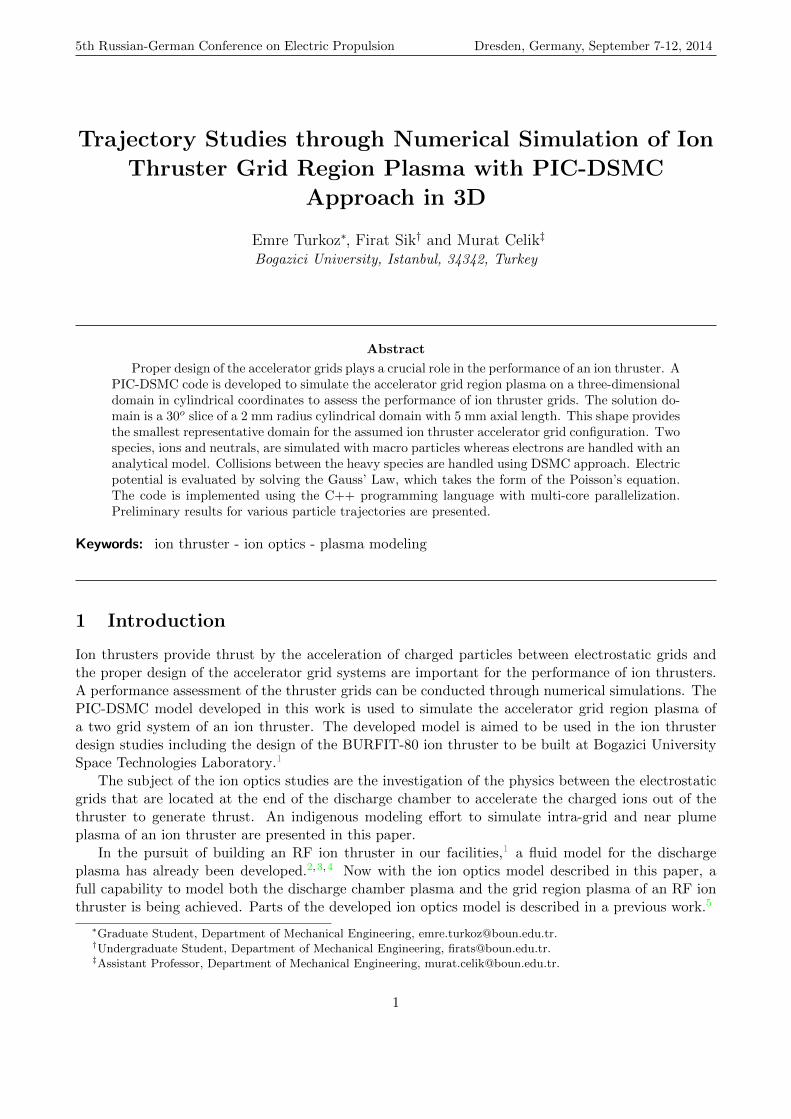
Figure 1: Representation of grid holes ofthe two-grid system11

In an ion thruster the acceleration of ions are achievedby the electrostatic potential difference applied between twoor more adjacent grids. In order explain the theory, a two-grid system, consisting of a screen and an accelerator grid,is investigated. A hole pair from screen and acceleratorgrids is shown in Figure 1.

Since ions directly affect the electric potential distribu-tion between the grids, the ion current extraction would berestricted by the Child-Langmuir space-charge limit, and itis formulated as:

J =4√

2

9ε0

(e

mi

)V

3/2a

l2g(1)

where lg is the gap distance between the grids, Va is theelectrostatic potential difference between the grids, ε0 is the permittivity of free space, e is the ele-mentary charge and mi is the mass of an ion.

If the space-charge limited current density is multiplied by the beam area, the maximum possiblecurrent can be calculated. For a beam with diameter D, the current is formulated as:

I =πD2

4J =

π

4

4√

2

9ε0

(e

mi

)D2

l2gV 3/2a = PV 3/2

a (2)

where P is called as the perveance of the extraction system. Taking into account the three-dimensionalgeometry effects, the following correction to calculate the perveance value is suggested:11

P =Ih

V3/2a

(leds

)(3)

where Ih is the beam current per hole, ds is the screen grid aperture diameter and le is defined as:

le =√l2g + (d2

s/4) (4)

2 Numerical Model

In this section, the implementation details of the developed ion optics code are presented. In theconsidered design, grids are assumed to be manufactured such that their holes are concentric withhexagons as shown in Fig. 2. A representation of the geometry where the plasma parameters areresolved in 3D is given in Fig. 2.

2


Figure 2: Ion grids geometry and the solution domain to be used in the model and presented with theintroduction of the igx9 ion optics code

2.1 Solving the Electric Potential

The equation solved to evaluate the electric potential distribution throughout the domain is thePoisson’s equation:

∇2φ = − ρ

ε0(5)

where ρ is the net charge density and ε0 is the permittivity of free space.For the wedge geometry presented in Fig. 2, a structured rectangular grid is used for the sides of

the 30o angle wedge for the computational study. The grid and an example boundary condition set ispresented in Fig. 3.

The electric potential equation (5) is extended to cylindrical coordinates as follows:

∇2φ =1

r

∂

∂r

(r∂φ

∂r

)+

1

r2

∂2φ

∂θ2+∂2φ

∂z2= − ρ

ε0(6)

where r denotes the radial coordinate. The right hand side of the equation, the charge density, is cal-culated by weighting each macroparticle’s charge to the cell nodes. According to the weighting schemeemployed in cylindrical coordinates, the accumulated charge at one node of the mesh is formulated asfollows

ρn = ρn +qpVcell

(1−|(zn − zp)π(r2

n − r2p)(θn − θp)|

Vcell

)(7)

where ρn denotes the charge density of the node, qp is the charge that the particle is carrying inCoulombs, and z, r and θ denotes the axial, radial and azimuthal coordinates, respectively. Use of ρnon both sides of the equation is done to indicate that this is actually a summation over each particle

Figure 3: Solution domain: Electric potential equation is solved in 3D cylindrical coordinates on a wedgeshaped domain with a 30o angle9

3


which is located in a cell that harbors this node. The subscript p denotes the particle and the subscriptn denotes the node considered. Vcell denotes the cell volume in cylindrical coordinates:

Vcell = π∆r(rL + rU )∆z∆θ (8)

where rL is the radial position of the lower node, and rU is the radial position of the upper node ofthe cell. Similarly, the weighting scheme is employed to interpolate the potential gradients calculatedon the mesh nodes to the particles. This scheme is as follows:

(∇φ)p = (∇φ)p + (∇φ)n

(1−|(zn − zp)π(r2

n − r2p)(θn − θp)|

Vcell

)(9)

By utilizing the weighting scheme, the total electric field on a macro particle is calculated with thecontribution coming from the 8 nodes that constitute the cell that the particle is located. In thisstudy, ions are tracked as macroparticles along with the neutral particles.

As stated, the solution domain is formulated in three dimensions, which are azimuthal, radial andaxial directions on a cylindrical coordinate system. To solve for the PDE for the electric potential, thesecond-order finite differencing scheme is applied to evaluate the coefficients. On a structured mesh,where the mesh sizes ∆r, ∆z, ∆θ are equal on the grid, the finite differencing scheme takes the formfor the central nodes:

∇2φ =φi−1,j,k − 2φi,j,k + φi+1,j,k

∆z2+φi,j−1,k − 2φi,j,k + φi,j+1,k

∆r2+φi,j,k−1 − 2φi,j,k + φi,j,k+1

r2∆θ2

+φi,j+1,k − φi,j−1,k

2∆r(10)

where i denotes the node index in the axial direction, j denotes the node index in the radial direction,and k denotes the node index in the azimuthal direction.

It can be observed from this expression that the potential of a node is directly affected by its 6neighboring nodes in each direction. The representation of these 6 neighboring nodes and 1 centernode is depicted in Fig. 4.

Figure 4: The 7-stencil secondorder finite differencing in three-dimensions

Let us call the number of nodes in the axial direction nz, num-ber of nodes in the radial direction nr on one azimuthal slice of thestructured grid in the 3D cylindrical coordinates. The numbering inFig. 4 starts from the back face neighbor of the center node, whichis denoted with the number 3. Between Node 0 and Node 3 there arenr× nz grid nodes. Node 1 denotes the radial neighbor on the southside, which has nz number node nodes in between with the Node 3.Node 2 is the west neighbor of the central node and one node behindthe Node 3, and Node 4 is the east neighbor of the central node andone node ahead. Node 5 is the north neighbor and nz number ofnodes ahead of Node 3. And Node 6 is the nr× nz grid nodes aheadof Node 3.

This numbering provides the opportunity to build a coefficient ma-trix that consists of nonzero diagonals and zero everywhere else. Thegenerated coefficient matrix has therefore a pentadiagonal sparsitypattern. The preferred sparse matrix storage scheme is compressed

diagonal storage (CDS) and it is implemented as described in.12 To solve these linearized systems,the utilization of an iterative solution scheme is mandatory. Jacobi, Gauss-Seidel,13 GMRES14 andILU preconditioned GMRES15 methods are implemented in the software framework as solvers. Thesesolvers are implemented considering the matrix storage scheme used. Among these solvers, it is ob-served that ILU-GMRES is the only one that can reduce the residual to the level below the desiredtolerance value within a reasonable computational time.

4


The electric field is calculated as the gradient of the potential:

E = −∇φ = −(∂φ

∂rr +

1

r

∂φ

∂θθ +

∂φ

∂zz

)(11)

After the electric potential and the electric field are evaluated, the ions move according to the forceapplied on them.5 The particle motion is performed with the commonly used Leapfrog algorithm.16

The collision are handled using DSMC approach as described in a previous work.5 DSMC collisionsare implemented with elastic collision cross sections obtained from the literature. Three types of heavyspecies collisions, Xe-Xe elastic, Xe-Xe+ elastic, and CEX collisions, are implemented.

2.2 Initializing Particles

Particle initialization is performed according to the assumption that particle velocities are distributedaccording to Maxwellian. Two particle species used in this work are ions and neutrals as stated before.Ions entering the domain from the discharge plasma have a drift velocity, which is equal to the Bohmvelocity in axial direction whereas neutrals move within the grid region without any directed velocity.But their initial velocity is always taken positive in the axial direction.

A probabilistic method is used to specify the velocity for the incoming particles. In the scope ofthis method, a distribution function, which is Maxwellian in our case, is used to represent particlevelocity probabilities: ∫ b

af(x)dx = 1 (12)

where a and b is the lower and upper limit of the velocities. Additional to this, a cumulative distributionfunction is introduced and defined as:

F (x) =

∫ x

af(x)dx (13)

The cumulative distribution function gives the integrals of the distribution function from the lowerlimit of the parameters to a given reference x value.

Maxwellian velocity distribution for a single direction is formulated as:

fv(vi) =

√m

2πkTexp

[−mv

2i

2kT

](14)

where m is the mass of the particle, k is the Boltzmann’s constant, T is the species temperature andvi is the velocity at a particular direction. If a particle has a directed drift velocity in a particulardirection, Maxwellian distribution takes the form:

fv(vi) =

√m

2πkTexp

[−m(vi − ai)2

2kT

](15)

where ai is the drift velocity in this direction. This form of the Maxwellian distribution is applied forions that enter the system with Bohm velocity.

A procedure is used to utilize these definitions and to find the probability of a particle having aspecified velocity. This procedure is named as Acceptance-Rejection Method. In this procedure, first arandom fraction, R1, is generated. A reference velocity value is then picked as vref = a+R1(b−a) fora specific particle. Then the value of the cumulative distribution function F (vref ) is calculated. Todetermine the probability that the particle has this velocity, a second random fraction, R2 is generated.If the new random fraction, R2, is larger than the cumulative distribution function value F (vref ), theparticle is assigned with the velocity vref . If the new random fraction, R2, is smaller than F (vref ),the process is repeated until the particle is assigned with the proper velocity component.

5


Figure 5: (a) Representation of the position change after axial reflection. (b) Representation of theposition change after radial reflection from the centerline. (c) Representation of the position change afterazimuthal reflection.

The problem configuration in this study requires also a little adjustment to the procedure describedabove. This adjustment will be explained after the details are given of the procedure to assign thepositions of the initialized particles. The routine that is used to determine the initial positions ofparticles are the same for ions and neutrals. We impose that both of these species are enteringthe system from the left boundary of the domain, at the axial coordinate, z = 0. The remainingtwo coordinates are calculated by using two random fractions in a very simple manner: The radialcoordinate of the particle, r = rmin + R1(rmax − rmin), whereas the azimuthal coordinate, θ =θmin +R2(θmax − θmin).

In the velocity assignment procedure, there is a slight difference between neutral and ion species.For the ions, the cumulative distribution function value is calculated assuming a drift velocity, whichis equal to the Bohm velocity, for Maxwellian distribution. For neutrals, the cumulative distributionfunction is calculated as usual with no directed drift velocity, so that the mean velocity is zero. Butthe assigned axial velocity is always positive for neutrals to prevent the unnecessary reflection in thefirst time step.

After velocity components are determined for each particle in the Cartesian (x, y, z) coordinates,these components are converted into the cylindrical coordinates (r, θ, z) and stored in this way. Sup-pose the velocity components in Cartesian coordinates are expressed as v = vxi + vy j + vzk. Their

counterparts in cylindrical coordinates are: v = vrr + vθθ + vz z. The transformation to cylindricalcoordinates is formulated as:

vz = vz (16)

vr = vxcos(θ) + vysin(θ) (17)

vθ = (−vxsin(θ) + vycos(θ))/r (18)

This transformation is performed for each particle initialized. It can be seen that the azimuthalvelocity component is stored as rad/s. It is converted into m/s when necessary by multiplying thisvalue with the radial coordinate of the particle.

2.3 Collisions with the Grid Walls

Collisions with the grid walls are handled so that particles colliding with the walls are reflected backinto the system with the same momentum.

6


The code implemented understands that a collision with grid walls occurred during the phasewhere the particles are relocated and reassigned to the cells they are located in. If a particle is foundto be located in one of the grid cells, its location and velocity are changed accordingly.

The reflection scheme is performed as represented in Figure 5. In this figure the shaded arearepresents the grid wall. A particle that has the position r at time t is marched in time with a specificvelocity and goes through a grid wall. During the particle reallocation process, the axial distancebetween the particle inside the grid and the grid wall is calculated. This value is shown with ∆z. Acalculation scheme is developed to understand whether the particle has entered from the left or rightside of the grid wall. According to this scheme, the distance of the particle to the both ends of thegrid is calculated. The distance of the particle to the left end is named as ∆zL, and the distance of theparticle to the right end is named as ∆zR. A representation of these distances is depicted in Figure5. So the following conditions apply to calculate the ∆z value to calculate new particle position:

If ∆zL < ∆zR then ∆z = ∆zL, if ∆zR < ∆zL then ∆z = −∆zR. The minus sign in the secondexpression is to take the direction of the coordinate system into account.

In this scheme it is assumed that the particle can not go through a distance that is equal to thehalf width of a grid within a time step.

Then the new position of the particle is calculated as:

rt+∆t = r′t+∆t − (2∆z)z (19)

The particle’s velocity is assumed to undergo a similar transformation, which will be explained below.The particle stores the velocity vector of the previous half-time step. If we express the calculatedvelocity as:

v′t+∆t/2 = rr + rθθ + zz (20)

Then the transformed velocity is:

v′t+∆t/2 = v′t+∆t/2 − 2zz (21)

Reflection from grids is performed during the loop over cells. The cells that fall on the gridlocations are tagged with a label, and the reflection is performed when there is a particle detected inthese cells.

2.4 Reflection: Particles Crossing the Radial Boundaries

Particles crossing the centerline (r = 0) and the top boundary (r = rmax) are handled with the simpleprinciple that for each particle leaving the domain, there should be another one entering the domainbecause of the axisymmetry.

The code implemented understands that a particle has crossed the centerline when its radialcoordinate obtains a negative value. Similarly if a particle has a radial coordinate larger than rmax,the particle is reflected from the top boundary.

The reflection scheme is performed as represented in Figure 5. In this figure the green arearepresents the region below the centerline where r < 0. A particle that has the position r at timet is marched in time with a specific velocity and goes below the centerline. During the particlereallocation process, the radial distance between the particle below the centerline and the centerlineitself is calculated. This value is shown with ∆r. Then the new position of the particle is calculatedas:

rt+∆t = r′t+∆t + (2∆r)r (22)

Similarly from the top boundary, the particle is reflected with the same formula given above, withthe ∆r value which is calculated as: ∆r = −(r′ − rmax). The minus sign is used to take the directionof the coordinate system into account.

7


The particle’s velocity is assumed to undergo a similar transformation. The particle stores thevelocity vector of the previous half-time step. If we express the calculated velocity as:

v′t+∆t/2 = rr + rθθ + zz (23)

Then the transformed velocity is:vt+∆t/2 = v′t+∆t/2 − 2rr (24)

Reflection from radial, azimuthal and the axial left boundaries is performed during the relocationof each particle to its corresponding cell. There is a routine at each time step to find the cells thatthe particles are located in after the motion from the previous time step. During this relocation, theparticles that cross the boundary are reflected back.

2.5 Reflection: Particles Crossing the Azimuthal Boundaries

Particles crossing the azimuthal boundaries (θ = 0 and θ = θmax) are handled assuming that for eachparticle that crosses the boundary, there is another one that enters the domain from the same locationdue to the symmetry condition.

The azimuthal reflection is depicted in Figure 5. The code implemented understands that a particlehas crossed the boundaries by doing an if-check on the θ coordinate of each particle. If θ coordinateis negative or larger than θmax, the reflection procedure is applied. The azimuthal coordinate of theparticle after the position is updated with the velocity is denoted with θ′t+∆t/2. In the scope of thisreflection, the following changes are performed on the azimuthal location and velocity of the macroparticle:

If θ′t+∆t/2 < 0:

θt+∆t/2 = θ′t+∆t/2 + 2∆θ (25)

where ∆θ = −θ′t+∆t/2. For the reflection from the other boundary, if θ′t+∆t/2 > θmax:

θt+∆t/2 = θend − 2∆θ (26)

where ∆θ = θ′t+∆t/2 − θmax.The velocity component at both boundaries is updated as follows. If we express the calculated

velocity as:v′t+∆t/2 = rr + rθθ + zz (27)

Then the transformed velocity is:

vt+∆t/2 = v′t+∆t/2 − 2rθθ (28)

3 Preliminary Results and Discussions

One of the domains investigated within the scope of this work is depicted in Figure 6. The purpose ofthe current study is to demonstrate the capabilities of the developed code such as particle tracking.The geometric configuration depicted in Figure 6 is held to be same at all simulation runs except forthe location of the acceleration grid, thus the distance between the two grids.

The solution domain is divided into 62 x 62 x 10 nodes, which are in axial, radial and azimuthaldirections, respectively. Poisson’s equation is solved to evaluate the electric potential. The evaluatedpotential field is used to calculate the electric field on the computational cell nodes and these valuesare then weighted on to each macroparticle to determine the resulting electric force.

The solution domain considered for the discussed runs are adapted from the work of Farnell.8 Themodeled domain is 5mm in axial direction and 2m in radial direction. The screen and acceleration

8


Figure 6: Dimensions of the solution domain for simulations

grids are set to 2241 V and -400 V, respectively. The potential in the plume region (right wall) isassumed to be at 0 V. The upstream discharge plasma potential is assumed to be 25 V above thescreen grid potential. The radial and azimuthal boundaries have symmetry boundary conditions.

Each macro particle is marched in time and a loop over particles locates the cells where eachparticle is located in. Each cell object contains a neutral and an ion particle list. Cell objects alsocontain flags to indicate whether they correspond to screen or accelerator grids, or they are boundarycells at the edges of the computational domain in three directions. If a particle gets into these cells,it is reflected while retaining its momentum as depicted in Figure 5. For the presented work only ionand neutral particles are assumed and the particle initialization is implemented as discussed in Section2.2.

A series of simulations are performed to investigate the particle trajectories and the flatness of thebeam, and perveance for a particular grid separation.

Initially, when there are no ions in the system, the Gauss’ Law reduces to the form of the Laplace’sequation. The resulting electric potential field is depicted in Figure 7. This solution indicates the

Figure 7: Electric potential fields in the solution domain at t=0 sec.

9


Figure 8: Distribution of the exit plane beam current for the discharge plasma ion number density:ni = 1.0e+ 16

existence of an almost uniform axial electric field between the screen and the accelerator grids.An important parameter in the ion grid system design is the radial current distribution of the ions

exiting the grid system. One of the goals is to keep the ions from hitting the grid walls and providinga low ion beam divergence. The ion beam current values through each computational cell at the exitplane (right boundary of the computational domain) are presented in Figure 8 for the bulk plasmadensity ni = 1.0e + 16 m−3. The desired profile for minimum beam divergence would have a smallwidth around the hole centerline.

Figure 9: Trajectories of arbitrary ion macro particles obtained from the PIC-DSMC model (the trajec-tories shown on the left appears as centerline reflections as depicted in the figure on the on the right)

One of the utilities of the presented PIC-DSMC code is the ability to track particles along theirshort journey within the solution domain. Randomly selected particles are tracked by printing theirradial and axial coordinates at each time-step. The azimuthal coordinates are not taken into accountbecause of the axisymmetry assumption in azimuthal direction. Some of the obtained trajectories aredepicted in Figure 9. As seen from the figure, use of the reflection at the centerline (r=0) boundary,the trajectories on the left figure can be represented as particles coming from the other side of thecenterline on the right figure.

10


The flatness of these trajectories would be a desirable design objective as it means a smaller beamdivergence and higher axial kinetic energy percentage. For example, particle #5 has velocity mostly inthe axial direction whereas particles #1 and #7 have significant radial velocity components and wouldcontribute to beam divergence angle to increase. Also, seen from the figure all particles, except forparticle #5, has trajectories that crosses the center axis and show the examples of centerline reflectionsfor the code as described in Section 2.4. Thus, to obtain an optimal configuration, the electric fieldtopology and the geometry has to be adjusted to adjust the cumulative of the ion particle trajectories.

Figure 10: Trajectories of arbitrary ion macro particles obtained from the PIC-DSMC model with analternative geometry configuration

As an alternative study, the geometry is changed slightly by moving the accelerator grid 0.6 mmto the right, thus making the grid separation distance 1.8 mm. Thus, different particle trajectoriesare obtained as few of which are shown in Figure 10. In this figure, the trajectory of the particle#4 shows that it undergoes an elastic collision with a neutral and as a result changes its trajectoryand hits the front side of the acceleration grid. In general, it is unlikely that an ion undergoes such alarge angle direction change due to an elastic collision with a neutral particle, however it is possible,and this trajectory is a suitable example of such a collision event. Additionally, particle #4 is also anexample of ions becoming neutrals when they interact with the grid walls.

4 Conclusion

A simulation platform to be used in the design of ion thruster grid systems is developed. The motionof macro particles is handled using the cylindrical coordinates in three-dimensions. The solutiondomain is chosen so that it represents the smallest symmetric section of a two-grid system that ismanufactured in a hexagonal pattern with circular concentric grid holes. The code is implementedusing the C++ programming language and uses the object oriented programming extensively. DSMCcollision algorithm is implemented to simulate the collisions between the heavy particle species.

The developed model will need additional capabilities such as improved handling of the electronsto simulate ion optics better as well as a sputtering model to increase its utility in ion thruster griddesign. Nevertheless, the model is a valuable tool for design and analysis of ion thruster grids.

Acknowledgment

This work was supported in part by The Scientific and Technological Research Council of Turkey underProjects TUBITAK-112M862 and TUBITAK-113M244 and in part by Bogazici University Scientific

11


Research Projects Support Fund under Projects BAP-6184 and BAP-8442.

References

[1] B. Yavuz, E. Turkoz, M. Celik, in 6th International Conference on Recent Advances in SpaceTechnologies (RAST), 619–624 (IEEE, 2013)

[2] E. Turkoz, M. Celik, in 49th Joint Propulsion Conference (San Jose, CA, 2013), also AIAA-2013-4110

[3] E. Turkoz, M. Celik, in 33rd International Electric Propulsion Conference (Washington DC, USA,2013), also IEPC-2013-294

[4] E. Turkoz, M. Celik, Plasma Science, IEEE Transactions on 42, 1, 235 (2014)

[5] E. Turkoz, F. Sik, M. Celik, in 50th Joint Propulsion Conference (Cleveland, OH, 2014), alsoAIAA-2014-3412

[6] J. R. Brophy, I. Katz, J. E. Polk, et al., AIAA Paper 4261, 2002 (2002)

[7] J. R. Anderson, I. Katz, D. Goebel, Numerical simulation of two-grid ion optics using a 3D code(Pasadena, CA: Jet Propulsion Laboratory, National Aeronautics and Space Administration,2004)

[8] C. Farnell, Performance and Lifetime Simulation of Ion Thruster Optics, Ph.D. Dissertation,Colorado State University, Fort Collins, CO, USA (2007)

[9] Y. Nakayama, P. J. Wilbur, in 27th International Electric Propulsion Conference (Pasadena, CA,2001), also IEPC-01-099

[10] M. Celik, M. M. Santi, S. Y. Cheng, et al., in 28th International Electric Propulsion Conference(Toulouse, France, 2003), also IEPC–03–134

[11] D. C. Rovang, P. Wilbur, Journal of Propulsion and Power 1, 3, 172 (1985)

[12] R. Barrett, M. W. Berry, T. F. Chan, et al., Templates for the Solution of Linear Systems:Building Blocks for Iterative Methods, vol. 43 (SIAM, 1994)

[13] L. Fausett, Applied Numerical Analysis Using MATLAB, Second Edition (Pearson Prentice Hall,2008)

[14] Y. Saad, M. H. Schultz, SIAM Journal on Scientific and Statistical Computing 7, 3, 856 (1986)

[15] J. Meijerink, H. A. van der Vorst, Mathematics of Computation 31, 137, 148 (1977)

[16] J. M. Fox, Advances in Fully-Kinetic PIC Simulations of a Near Vacuum Hall Thruster and OtherPlasma Systems, Ph.D. Thesis, Massachusetts Institute of Technology, Cambridge, USA (2007)

12

Trajectory Studies through Numerical Simulation of Ion ...

Documents

Transcript of Trajectory Studies through Numerical Simulation of Ion ...