Journal of Physics Conference Series

OPEN ACCESS

Trajectory control with continuous thrust applied toa rendezvous maneuverTo cite this article W G Santos and E M Rocco 2013 J Phys Conf Ser 465 012021

View the article online for updates and enhancements

You may also likeSoft docking with damping of twospacecraft using a tetherV S Aslanov and R S Pikalov

-

A Fast and AdaptiveMAAPS Multi-RadioRendezvous Algorithm for CognitiveRadio NetworksMrs R Gomathi Ms S Kalpana and Ms NSaropriya

-

Optimal mission planning for refuellingLEO satellites with peer-to-peer strategyJing Yu and Dong Hao

-

This content was downloaded from IP address 4670219125 on 14012022 at 2019

Trajectory control with continuous thrust applied to

a rendezvous maneuver

W G Santos and E M Rocco

National Institute for Space Research Space Mechanics and Control Division Sao Jose dosCampos Brazil

E-mail willergomesdeminpebr

Abstract A rendezvous mission can be divided into the following phases launch phasingfar range rendezvous close range rendezvous and mating (docking or berthing) This paperaims to present a close range rendezvous with closed loop controlled straight line trajectoryThe approaching is executed on V-bar axis A PID controller and continuous thrust are usedto eliminate the residual errors in the trajectory A comparative study about the linear andnonlinear dynamics is performed and the results showed that the linear equations becomeinaccurate insofar as the chaser moves away from the target

1 IntroductionRendezvous and docking or berthing (RVDB) technology are key elements in mission such asassembly in orbit of larger units re-supply of orbital platforms and stations exchange of crewin orbital stations repair of spacecraft in orbit retrieval of spacecraft and others The RVDBprocess includes several orbital maneuvers and trajectory control On 16 March 1966 took placethe first rendezvous and docking between two spacecrafts and the first automatic RVD tookplace only on 30 October 1967 A rendezvous mission can be divided into a number of phaseslaunch phasing far range rendezvous close range rendezvous and mating

This paper will focus on close range rendezvous phase which can be divided into two sub-phases a preparatory phase leading to the final approach corridor often called closing anda final approach phase leading to the mating conditions The objectives of the closing phaseare the reduction of the range to the target and the achievement of conditions allowing theacquisition of the final approach corridor Different acquisition strategies for V-bar and R-barapproaches can be executed The objective of the final approach phase is to achieve dockingor berthing capture conditions in terms of positions and velocities and of relative attitude andangular rates The straight line or the quasi-straight line trajectory are used in this maneuverphase The guidance navigation and control (GNC) system of the chaser must following thedirection of the target docking axes To meet this requirement the relative attitude betweenthe docking ports of the two spacecrafts should be measured and taken to zero at the end ofthe maneuver For observability and safe reasons a cone-shaped approach corridor will usuallybe defined within which the approach trajectory has to remain This corridor has a half coneangle of 10-15 deg [1]

A comparison between a linear dynamics model - take into account a circular orbit - and anonlinear dynamics model - for an orbit with eccentricity of 01 - was done by [2] Although his

XVI Brazilian Colloquium on Orbital Dynamics IOP PublishingJournal of Physics Conference Series 465 (2013) 012021 doi1010881742-65964651012021

Content from this work may be used under the terms of the Creative Commons Attribution 30 licence Any further distributionof this work must maintain attribution to the author(s) and the title of the work journal citation and DOI

Published under licence by IOP Publishing Ltd 1

main intention was present a new method for applying the Hill equations to the elliptical orbitsthis comparative study is a valuable reference So the purposes of this paper are the followinganalyze the relative motion for several initial conditions find out the difference between the linearand nonlinear spacecraft dynamics considering the same orbital eccentricity and to perform aclose range rendezvous with closed loop controlled straight line trajectory on V-bar axis TheSection 2 shows the equations of the control system The simulations and results are shown inSection 3 Lastly a conclusion is given in Section 4

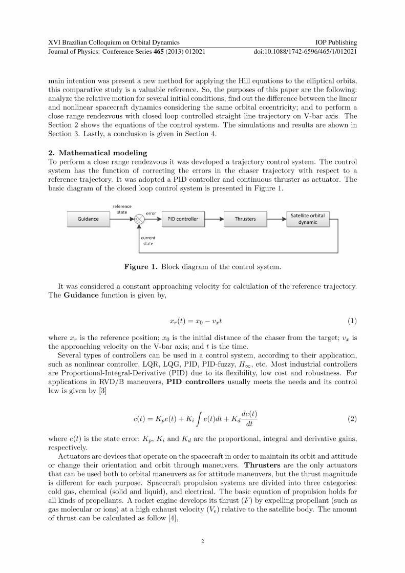
2 Mathematical modelingTo perform a close range rendezvous it was developed a trajectory control system The controlsystem has the function of correcting the errors in the chaser trajectory with respect to areference trajectory It was adopted a PID controller and continuous thruster as actuator Thebasic diagram of the closed loop control system is presented in Figure 1

Figure 1 Block diagram of the control system

It was considered a constant approaching velocity for calculation of the reference trajectoryThe Guidance function is given by

xr(t) = x0 minus vxt (1)

where xr is the reference position x0 is the initial distance of the chaser from the target vx isthe approaching velocity on the V-bar axis and t is the time

Several types of controllers can be used in a control system according to their applicationsuch as nonlinear controller LQR LQG PID PID-fuzzy Hinfin etc Most industrial controllersare Proportional-Integral-Derivative (PID) due to its flexibility low cost and robustness Forapplications in RVDB maneuvers PID controllers usually meets the needs and its controllaw is given by [3]

c(t) = Kpe(t) +Ki

inte(t)dt+Kd

de(t)

dt(2)

where e(t) is the state error Kp Ki and Kd are the proportional integral and derivative gainsrespectively

Actuators are devices that operate on the spacecraft in order to maintain its orbit and attitudeor change their orientation and orbit through maneuvers Thrusters are the only actuatorsthat can be used both to orbital maneuvers as for attitude maneuvers but the thrust magnitudeis different for each purpose Spacecraft propulsion systems are divided into three categoriescold gas chemical (solid and liquid) and electrical The basic equation of propulsion holds forall kinds of propellants A rocket engine develops its thrust (F ) by expelling propellant (such asgas molecular or ions) at a high exhaust velocity (Ve) relative to the satellite body The amountof thrust can be calculated as follow [4]

XVI Brazilian Colloquium on Orbital Dynamics IOP PublishingJournal of Physics Conference Series 465 (2013) 012021 doi1010881742-65964651012021

2

F = Vedm

dt+Ae[Pe minus Pa] = Vef

dm

dt(3)

where Pe and Pa are the gas and ambient pressures respectively Ve is the exhaust velocity Vefis the effective exhaust velocity of the expelled mass with respect to the satellite dmdt is themass flow rate of the propellant and Ae denotes the area of the nozzle exit

During the close range rendezvous the chaser is a few tens of meters from the target andtherewith the relative navigation assumes greater importance The following considerations aretaken in the development of equations the spacecraft is treated as a mass point the chasermotion is disturbed by the effects of spherical earths gravitational fields and the thruster forcesConsider X Y and Z as axis of the inertial frame x y and z are the axis of the target centeredlocal orbital frame rc and rt is vector radius of the chaser and target respectively as shown inFigure 2 In the rendezvous literature the x axis y axis and z axis is called by V-bar H-barand R-bar respectively

Figure 2 Local orbital frame and inertial frame

The relative acceleration s is

s = rc minus rt (4)

The general equations for motion under the influence of a central force are written as [1]

rt = minusmicro rtr3t

(5)

rc = minusmicrorcr3c

+ fu

where micro is the earthrsquos gravitational constant and fu is the specific force vector of control Theequations 4 and 5 represent the nonlinear dynamics of the system

The target centered local orbital frame is a non-inertial frame and it is rotating around thecentral body with an orbital rate ω It is common to express the relative motion by linear timevarying differential equations as shown in [1]

XVI Brazilian Colloquium on Orbital Dynamics IOP PublishingJournal of Physics Conference Series 465 (2013) 012021 doi1010881742-65964651012021

3

xminus 2ωz = fx

y + ω2y = fy (6)

z + 2ωxminus 3ω2z = fz

where ω is the orbital angular velocity that for the special case of circular orbits is consideredconstant and can be expressed by

ω2 =micro

r3t(7)

and fx fy and fz are the components of the specific force vector of controlThe Equations 6 represent the linear dynamics of the relative motion and are known as

Hill equations The derivation of these equations starts from the linearization of the nonlinearequations and can be consulted in [1] and [5]

3 ResultsThis section will present the results about the relative motion between two spacecrafts Twostudy cases were prepared the first shows the relative motion dynamic for different initialconditions of the chaser vehicle a comparison of the nonlinear and linear dynamics is performedin order to identify the error originating from the linearization and the second case illustrates arendezvous maneuver considering closed loop controlled straight line trajectory All results arepresented in the target centered local orbital frame

It was used a simulation step of 1 second The initial keplerian elements of the target vehicleare shown in Table 1

Table 1 Initial conditions of the target

Parameter Value

Altitude (km) 400Eccentricity 0Inclination (degrees) 30RAAN (degrees) 0Perigee argument (degrees) 0Mean anomaly (degrees) 10

31 Case 1 Analysis of the relative motion dynamicsIn this first case the relative motion of the linear and nonlinear dynamics was evaluated fortwo orbits of the target The initial condition of the chaser is shown in the legend of eachfigure The first situation is considered with the chaser starting at 10 m away from the targetin the direction of the R-bar axis the relative motion can be seen in the Figure 3 It can beobserved that after two orbits the chaser is approximately 750 m away from the target Inorder to evaluate the error from the linearization the Figure 4 presents the difference betweenthe models considering the initial conditions of the Figure 3 as a function of target distanceExceptionally in this graph the stopping criterion was changed to four orbits of the target It

XVI Brazilian Colloquium on Orbital Dynamics IOP PublishingJournal of Physics Conference Series 465 (2013) 012021 doi1010881742-65964651012021

4

Figure 3 Case 1 x0 y0 = 0 z0 = 10 mx0 y0 z0 = 0

Figure 4 Case 1 (difference between themodels) x0 y0 = 0 z0 = 10 m x0 y0 z0 =0

is noted that the Hill equations lose their accuracy since the distance between the spacecraftsincreases reaching an error of the order of 1 m in 1500 km from the target

Consider that the spacecrafts are coupled and the chaser is subjected to a impulse ofmagnitude of 001 ms in the direction of +V-bar ie a impulsive ∆V in the tangential directionto the orbit The resulting movement is depicted in Figure 5 Now the same impulse is appliedhowever in the radial direction to the orbit ie toward +R-bar The relative dynamic behaviorin this case can be seen in Figure 6 The resulting trajectory is an ellipse that is the spacecraftreturns to the initial position each orbital revolution From the Figures 5 and 6 we can concludethat the displacements due to a radial ∆V are much smaller than those due to a tangential ∆Vof the same size

Figure 5 Case 1 x0 y0 z0 = 0 x0 =001 ms y0 z0 = 0

Figure 6 Case 1 x0 y0 z0 = 0 z0 =001 ms x0 y0 = 0

The relative motion considering the initial condition of 10 m in the H-bar axis as a functionof time is presented in the Figure 7 We can highlight the sinusoidal behavior of the motionwhen the vehicle starts from a point outside the orbital plane

32 Case 2 Close range rendezvous with closed loop controlled straight line trajectoryIn this second case it was considered a trajectory control system to perform a close rangerendezvous in the V-bar axis The chaser is 100 m from the target in the V-bar direction and itis wanted to perform the rendezvous with a constant velocity of 005 ms The Figure 8 showsthe transitory response with the linear and nonlinear dynamics The movement in each axis asfunction of time is presented in Figure 9 It is observed that in the V-bar axis the vehicle hasmet the target at a constant velocity as desired movement on the H-bar axis is not occurredbecause there was not application of forces outside the orbital plane and there was a deviationin the R-bar axis due to coupling between the R-bar and V-bar axis

XVI Brazilian Colloquium on Orbital Dynamics IOP PublishingJournal of Physics Conference Series 465 (2013) 012021 doi1010881742-65964651012021

5

Figure 7 Case 1 x0 z0 = 0 y0 = 10 m x0 y0 z0 = 0

Figure 8 Case 2 (R-bar times V-bar) x0 =100 m y0 z0 = 0 x0 y0 z0 = 0 vx = 005ms

Figure 9 Case 2 (separated by axes) x0 =100 m y0 z0 = 0 x0 y0 z0 = 0 vx = 005ms

4 ConclusionsThis paper presented a study about rendezvous maneuver In the first case free drift motionand impulsive maneuvers were analyzed for several initial conditions The divergence betweenthe linear and nonlinear spacecraft dynamics were also investigated The second case showedthe application of the trajectory control system in a close range rendezvous The first resultsindicated that an specific motion can be yielded for each initial condition like a sinusoidal radialor cyclic behavior Because of the linearization the Hill equations become inaccurate insofaras the chaser moves away from the target So for long distances the nonlinear model is mostadvisable Although we have different transitory responses the trajectory control system metthe requirements and executed the close range rendezvous with both models

References[1] Fehse W 2003 Automated rendezvous and docking of spacecraft (New York USA Cambridge University Press)

495[2] Yamanaka K and Ankersen F 2002 New state transition matrix for relative motion on an arbitrary elliptical

orbit J Guid Control Dynam 25 60-66[3] Ogata K 1970 Modern control engineering (Englewood Cliffs NJ Prentice-Hall) 836[4] Sidi M J 1997 Spacecraft dynamics and control A practical engineering approach (New York USA Cambridge

University Press) 409[5] Arantes Jr G and Rocco E M and Komanduri A S 2010 Far and close approaching strategies for rendezvous

and docking operations applied to on-orbit servicing (Mathematical analysis and applications in engineeringaerospace and sciences vol 5) ed S Sivasundaram (USA Cambridge Scientific) pp 1-29

XVI Brazilian Colloquium on Orbital Dynamics IOP PublishingJournal of Physics Conference Series 465 (2013) 012021 doi1010881742-65964651012021

6

main intention was present a new method for applying the Hill equations to the elliptical orbitsthis comparative study is a valuable reference So the purposes of this paper are the followinganalyze the relative motion for several initial conditions find out the difference between the linearand nonlinear spacecraft dynamics considering the same orbital eccentricity and to perform aclose range rendezvous with closed loop controlled straight line trajectory on V-bar axis TheSection 2 shows the equations of the control system The simulations and results are shown inSection 3 Lastly a conclusion is given in Section 4

2 Mathematical modelingTo perform a close range rendezvous it was developed a trajectory control system The controlsystem has the function of correcting the errors in the chaser trajectory with respect to areference trajectory It was adopted a PID controller and continuous thruster as actuator Thebasic diagram of the closed loop control system is presented in Figure 1

Figure 1 Block diagram of the control system

It was considered a constant approaching velocity for calculation of the reference trajectoryThe Guidance function is given by

xr(t) = x0 minus vxt (1)

where xr is the reference position x0 is the initial distance of the chaser from the target vx isthe approaching velocity on the V-bar axis and t is the time

Several types of controllers can be used in a control system according to their applicationsuch as nonlinear controller LQR LQG PID PID-fuzzy Hinfin etc Most industrial controllersare Proportional-Integral-Derivative (PID) due to its flexibility low cost and robustness Forapplications in RVDB maneuvers PID controllers usually meets the needs and its controllaw is given by [3]

c(t) = Kpe(t) +Ki

inte(t)dt+Kd

de(t)

dt(2)

where e(t) is the state error Kp Ki and Kd are the proportional integral and derivative gainsrespectively

Actuators are devices that operate on the spacecraft in order to maintain its orbit and attitudeor change their orientation and orbit through maneuvers Thrusters are the only actuatorsthat can be used both to orbital maneuvers as for attitude maneuvers but the thrust magnitudeis different for each purpose Spacecraft propulsion systems are divided into three categoriescold gas chemical (solid and liquid) and electrical The basic equation of propulsion holds forall kinds of propellants A rocket engine develops its thrust (F ) by expelling propellant (such asgas molecular or ions) at a high exhaust velocity (Ve) relative to the satellite body The amountof thrust can be calculated as follow [4]

XVI Brazilian Colloquium on Orbital Dynamics IOP PublishingJournal of Physics Conference Series 465 (2013) 012021 doi1010881742-65964651012021

2

F = Vedm

dt+Ae[Pe minus Pa] = Vef

dm

dt(3)

where Pe and Pa are the gas and ambient pressures respectively Ve is the exhaust velocity Vefis the effective exhaust velocity of the expelled mass with respect to the satellite dmdt is themass flow rate of the propellant and Ae denotes the area of the nozzle exit

During the close range rendezvous the chaser is a few tens of meters from the target andtherewith the relative navigation assumes greater importance The following considerations aretaken in the development of equations the spacecraft is treated as a mass point the chasermotion is disturbed by the effects of spherical earths gravitational fields and the thruster forcesConsider X Y and Z as axis of the inertial frame x y and z are the axis of the target centeredlocal orbital frame rc and rt is vector radius of the chaser and target respectively as shown inFigure 2 In the rendezvous literature the x axis y axis and z axis is called by V-bar H-barand R-bar respectively

Figure 2 Local orbital frame and inertial frame

The relative acceleration s is

s = rc minus rt (4)

The general equations for motion under the influence of a central force are written as [1]

rt = minusmicro rtr3t

(5)

rc = minusmicrorcr3c

+ fu

where micro is the earthrsquos gravitational constant and fu is the specific force vector of control Theequations 4 and 5 represent the nonlinear dynamics of the system

The target centered local orbital frame is a non-inertial frame and it is rotating around thecentral body with an orbital rate ω It is common to express the relative motion by linear timevarying differential equations as shown in [1]

XVI Brazilian Colloquium on Orbital Dynamics IOP PublishingJournal of Physics Conference Series 465 (2013) 012021 doi1010881742-65964651012021

3

xminus 2ωz = fx

y + ω2y = fy (6)

z + 2ωxminus 3ω2z = fz

where ω is the orbital angular velocity that for the special case of circular orbits is consideredconstant and can be expressed by

ω2 =micro

r3t(7)

and fx fy and fz are the components of the specific force vector of controlThe Equations 6 represent the linear dynamics of the relative motion and are known as

Hill equations The derivation of these equations starts from the linearization of the nonlinearequations and can be consulted in [1] and [5]

3 ResultsThis section will present the results about the relative motion between two spacecrafts Twostudy cases were prepared the first shows the relative motion dynamic for different initialconditions of the chaser vehicle a comparison of the nonlinear and linear dynamics is performedin order to identify the error originating from the linearization and the second case illustrates arendezvous maneuver considering closed loop controlled straight line trajectory All results arepresented in the target centered local orbital frame

It was used a simulation step of 1 second The initial keplerian elements of the target vehicleare shown in Table 1

Table 1 Initial conditions of the target

Parameter Value

Altitude (km) 400Eccentricity 0Inclination (degrees) 30RAAN (degrees) 0Perigee argument (degrees) 0Mean anomaly (degrees) 10

31 Case 1 Analysis of the relative motion dynamicsIn this first case the relative motion of the linear and nonlinear dynamics was evaluated fortwo orbits of the target The initial condition of the chaser is shown in the legend of eachfigure The first situation is considered with the chaser starting at 10 m away from the targetin the direction of the R-bar axis the relative motion can be seen in the Figure 3 It can beobserved that after two orbits the chaser is approximately 750 m away from the target Inorder to evaluate the error from the linearization the Figure 4 presents the difference betweenthe models considering the initial conditions of the Figure 3 as a function of target distanceExceptionally in this graph the stopping criterion was changed to four orbits of the target It

XVI Brazilian Colloquium on Orbital Dynamics IOP PublishingJournal of Physics Conference Series 465 (2013) 012021 doi1010881742-65964651012021

4

Figure 3 Case 1 x0 y0 = 0 z0 = 10 mx0 y0 z0 = 0

Figure 4 Case 1 (difference between themodels) x0 y0 = 0 z0 = 10 m x0 y0 z0 =0

is noted that the Hill equations lose their accuracy since the distance between the spacecraftsincreases reaching an error of the order of 1 m in 1500 km from the target

Consider that the spacecrafts are coupled and the chaser is subjected to a impulse ofmagnitude of 001 ms in the direction of +V-bar ie a impulsive ∆V in the tangential directionto the orbit The resulting movement is depicted in Figure 5 Now the same impulse is appliedhowever in the radial direction to the orbit ie toward +R-bar The relative dynamic behaviorin this case can be seen in Figure 6 The resulting trajectory is an ellipse that is the spacecraftreturns to the initial position each orbital revolution From the Figures 5 and 6 we can concludethat the displacements due to a radial ∆V are much smaller than those due to a tangential ∆Vof the same size

Figure 5 Case 1 x0 y0 z0 = 0 x0 =001 ms y0 z0 = 0

Figure 6 Case 1 x0 y0 z0 = 0 z0 =001 ms x0 y0 = 0

The relative motion considering the initial condition of 10 m in the H-bar axis as a functionof time is presented in the Figure 7 We can highlight the sinusoidal behavior of the motionwhen the vehicle starts from a point outside the orbital plane

32 Case 2 Close range rendezvous with closed loop controlled straight line trajectoryIn this second case it was considered a trajectory control system to perform a close rangerendezvous in the V-bar axis The chaser is 100 m from the target in the V-bar direction and itis wanted to perform the rendezvous with a constant velocity of 005 ms The Figure 8 showsthe transitory response with the linear and nonlinear dynamics The movement in each axis asfunction of time is presented in Figure 9 It is observed that in the V-bar axis the vehicle hasmet the target at a constant velocity as desired movement on the H-bar axis is not occurredbecause there was not application of forces outside the orbital plane and there was a deviationin the R-bar axis due to coupling between the R-bar and V-bar axis

XVI Brazilian Colloquium on Orbital Dynamics IOP PublishingJournal of Physics Conference Series 465 (2013) 012021 doi1010881742-65964651012021

5

Figure 7 Case 1 x0 z0 = 0 y0 = 10 m x0 y0 z0 = 0

Figure 8 Case 2 (R-bar times V-bar) x0 =100 m y0 z0 = 0 x0 y0 z0 = 0 vx = 005ms

Figure 9 Case 2 (separated by axes) x0 =100 m y0 z0 = 0 x0 y0 z0 = 0 vx = 005ms

4 ConclusionsThis paper presented a study about rendezvous maneuver In the first case free drift motionand impulsive maneuvers were analyzed for several initial conditions The divergence betweenthe linear and nonlinear spacecraft dynamics were also investigated The second case showedthe application of the trajectory control system in a close range rendezvous The first resultsindicated that an specific motion can be yielded for each initial condition like a sinusoidal radialor cyclic behavior Because of the linearization the Hill equations become inaccurate insofaras the chaser moves away from the target So for long distances the nonlinear model is mostadvisable Although we have different transitory responses the trajectory control system metthe requirements and executed the close range rendezvous with both models

References[1] Fehse W 2003 Automated rendezvous and docking of spacecraft (New York USA Cambridge University Press)

495[2] Yamanaka K and Ankersen F 2002 New state transition matrix for relative motion on an arbitrary elliptical

orbit J Guid Control Dynam 25 60-66[3] Ogata K 1970 Modern control engineering (Englewood Cliffs NJ Prentice-Hall) 836[4] Sidi M J 1997 Spacecraft dynamics and control A practical engineering approach (New York USA Cambridge

University Press) 409[5] Arantes Jr G and Rocco E M and Komanduri A S 2010 Far and close approaching strategies for rendezvous

and docking operations applied to on-orbit servicing (Mathematical analysis and applications in engineeringaerospace and sciences vol 5) ed S Sivasundaram (USA Cambridge Scientific) pp 1-29

XVI Brazilian Colloquium on Orbital Dynamics IOP PublishingJournal of Physics Conference Series 465 (2013) 012021 doi1010881742-65964651012021

6

F = Vedm

dt+Ae[Pe minus Pa] = Vef

dm

dt(3)

where Pe and Pa are the gas and ambient pressures respectively Ve is the exhaust velocity Vefis the effective exhaust velocity of the expelled mass with respect to the satellite dmdt is themass flow rate of the propellant and Ae denotes the area of the nozzle exit

During the close range rendezvous the chaser is a few tens of meters from the target andtherewith the relative navigation assumes greater importance The following considerations aretaken in the development of equations the spacecraft is treated as a mass point the chasermotion is disturbed by the effects of spherical earths gravitational fields and the thruster forcesConsider X Y and Z as axis of the inertial frame x y and z are the axis of the target centeredlocal orbital frame rc and rt is vector radius of the chaser and target respectively as shown inFigure 2 In the rendezvous literature the x axis y axis and z axis is called by V-bar H-barand R-bar respectively

Figure 2 Local orbital frame and inertial frame

The relative acceleration s is

s = rc minus rt (4)

The general equations for motion under the influence of a central force are written as [1]

rt = minusmicro rtr3t

(5)

rc = minusmicrorcr3c

+ fu

where micro is the earthrsquos gravitational constant and fu is the specific force vector of control Theequations 4 and 5 represent the nonlinear dynamics of the system

The target centered local orbital frame is a non-inertial frame and it is rotating around thecentral body with an orbital rate ω It is common to express the relative motion by linear timevarying differential equations as shown in [1]

XVI Brazilian Colloquium on Orbital Dynamics IOP PublishingJournal of Physics Conference Series 465 (2013) 012021 doi1010881742-65964651012021

3

xminus 2ωz = fx

y + ω2y = fy (6)

z + 2ωxminus 3ω2z = fz

where ω is the orbital angular velocity that for the special case of circular orbits is consideredconstant and can be expressed by

ω2 =micro

r3t(7)

and fx fy and fz are the components of the specific force vector of controlThe Equations 6 represent the linear dynamics of the relative motion and are known as

Hill equations The derivation of these equations starts from the linearization of the nonlinearequations and can be consulted in [1] and [5]

3 ResultsThis section will present the results about the relative motion between two spacecrafts Twostudy cases were prepared the first shows the relative motion dynamic for different initialconditions of the chaser vehicle a comparison of the nonlinear and linear dynamics is performedin order to identify the error originating from the linearization and the second case illustrates arendezvous maneuver considering closed loop controlled straight line trajectory All results arepresented in the target centered local orbital frame

It was used a simulation step of 1 second The initial keplerian elements of the target vehicleare shown in Table 1

Table 1 Initial conditions of the target

Parameter Value

Altitude (km) 400Eccentricity 0Inclination (degrees) 30RAAN (degrees) 0Perigee argument (degrees) 0Mean anomaly (degrees) 10

31 Case 1 Analysis of the relative motion dynamicsIn this first case the relative motion of the linear and nonlinear dynamics was evaluated fortwo orbits of the target The initial condition of the chaser is shown in the legend of eachfigure The first situation is considered with the chaser starting at 10 m away from the targetin the direction of the R-bar axis the relative motion can be seen in the Figure 3 It can beobserved that after two orbits the chaser is approximately 750 m away from the target Inorder to evaluate the error from the linearization the Figure 4 presents the difference betweenthe models considering the initial conditions of the Figure 3 as a function of target distanceExceptionally in this graph the stopping criterion was changed to four orbits of the target It

XVI Brazilian Colloquium on Orbital Dynamics IOP PublishingJournal of Physics Conference Series 465 (2013) 012021 doi1010881742-65964651012021

4

Figure 3 Case 1 x0 y0 = 0 z0 = 10 mx0 y0 z0 = 0

Figure 4 Case 1 (difference between themodels) x0 y0 = 0 z0 = 10 m x0 y0 z0 =0

is noted that the Hill equations lose their accuracy since the distance between the spacecraftsincreases reaching an error of the order of 1 m in 1500 km from the target

Consider that the spacecrafts are coupled and the chaser is subjected to a impulse ofmagnitude of 001 ms in the direction of +V-bar ie a impulsive ∆V in the tangential directionto the orbit The resulting movement is depicted in Figure 5 Now the same impulse is appliedhowever in the radial direction to the orbit ie toward +R-bar The relative dynamic behaviorin this case can be seen in Figure 6 The resulting trajectory is an ellipse that is the spacecraftreturns to the initial position each orbital revolution From the Figures 5 and 6 we can concludethat the displacements due to a radial ∆V are much smaller than those due to a tangential ∆Vof the same size

Figure 5 Case 1 x0 y0 z0 = 0 x0 =001 ms y0 z0 = 0

Figure 6 Case 1 x0 y0 z0 = 0 z0 =001 ms x0 y0 = 0

The relative motion considering the initial condition of 10 m in the H-bar axis as a functionof time is presented in the Figure 7 We can highlight the sinusoidal behavior of the motionwhen the vehicle starts from a point outside the orbital plane

32 Case 2 Close range rendezvous with closed loop controlled straight line trajectoryIn this second case it was considered a trajectory control system to perform a close rangerendezvous in the V-bar axis The chaser is 100 m from the target in the V-bar direction and itis wanted to perform the rendezvous with a constant velocity of 005 ms The Figure 8 showsthe transitory response with the linear and nonlinear dynamics The movement in each axis asfunction of time is presented in Figure 9 It is observed that in the V-bar axis the vehicle hasmet the target at a constant velocity as desired movement on the H-bar axis is not occurredbecause there was not application of forces outside the orbital plane and there was a deviationin the R-bar axis due to coupling between the R-bar and V-bar axis

XVI Brazilian Colloquium on Orbital Dynamics IOP PublishingJournal of Physics Conference Series 465 (2013) 012021 doi1010881742-65964651012021

5

Figure 7 Case 1 x0 z0 = 0 y0 = 10 m x0 y0 z0 = 0

Figure 8 Case 2 (R-bar times V-bar) x0 =100 m y0 z0 = 0 x0 y0 z0 = 0 vx = 005ms

Figure 9 Case 2 (separated by axes) x0 =100 m y0 z0 = 0 x0 y0 z0 = 0 vx = 005ms

4 ConclusionsThis paper presented a study about rendezvous maneuver In the first case free drift motionand impulsive maneuvers were analyzed for several initial conditions The divergence betweenthe linear and nonlinear spacecraft dynamics were also investigated The second case showedthe application of the trajectory control system in a close range rendezvous The first resultsindicated that an specific motion can be yielded for each initial condition like a sinusoidal radialor cyclic behavior Because of the linearization the Hill equations become inaccurate insofaras the chaser moves away from the target So for long distances the nonlinear model is mostadvisable Although we have different transitory responses the trajectory control system metthe requirements and executed the close range rendezvous with both models

References[1] Fehse W 2003 Automated rendezvous and docking of spacecraft (New York USA Cambridge University Press)

495[2] Yamanaka K and Ankersen F 2002 New state transition matrix for relative motion on an arbitrary elliptical

orbit J Guid Control Dynam 25 60-66[3] Ogata K 1970 Modern control engineering (Englewood Cliffs NJ Prentice-Hall) 836[4] Sidi M J 1997 Spacecraft dynamics and control A practical engineering approach (New York USA Cambridge

University Press) 409[5] Arantes Jr G and Rocco E M and Komanduri A S 2010 Far and close approaching strategies for rendezvous

and docking operations applied to on-orbit servicing (Mathematical analysis and applications in engineeringaerospace and sciences vol 5) ed S Sivasundaram (USA Cambridge Scientific) pp 1-29

XVI Brazilian Colloquium on Orbital Dynamics IOP PublishingJournal of Physics Conference Series 465 (2013) 012021 doi1010881742-65964651012021

6

xminus 2ωz = fx

y + ω2y = fy (6)

z + 2ωxminus 3ω2z = fz

where ω is the orbital angular velocity that for the special case of circular orbits is consideredconstant and can be expressed by

ω2 =micro

r3t(7)

and fx fy and fz are the components of the specific force vector of controlThe Equations 6 represent the linear dynamics of the relative motion and are known as

Hill equations The derivation of these equations starts from the linearization of the nonlinearequations and can be consulted in [1] and [5]

3 ResultsThis section will present the results about the relative motion between two spacecrafts Twostudy cases were prepared the first shows the relative motion dynamic for different initialconditions of the chaser vehicle a comparison of the nonlinear and linear dynamics is performedin order to identify the error originating from the linearization and the second case illustrates arendezvous maneuver considering closed loop controlled straight line trajectory All results arepresented in the target centered local orbital frame

It was used a simulation step of 1 second The initial keplerian elements of the target vehicleare shown in Table 1

Table 1 Initial conditions of the target

Parameter Value

Altitude (km) 400Eccentricity 0Inclination (degrees) 30RAAN (degrees) 0Perigee argument (degrees) 0Mean anomaly (degrees) 10

31 Case 1 Analysis of the relative motion dynamicsIn this first case the relative motion of the linear and nonlinear dynamics was evaluated fortwo orbits of the target The initial condition of the chaser is shown in the legend of eachfigure The first situation is considered with the chaser starting at 10 m away from the targetin the direction of the R-bar axis the relative motion can be seen in the Figure 3 It can beobserved that after two orbits the chaser is approximately 750 m away from the target Inorder to evaluate the error from the linearization the Figure 4 presents the difference betweenthe models considering the initial conditions of the Figure 3 as a function of target distanceExceptionally in this graph the stopping criterion was changed to four orbits of the target It

XVI Brazilian Colloquium on Orbital Dynamics IOP PublishingJournal of Physics Conference Series 465 (2013) 012021 doi1010881742-65964651012021

4

Figure 3 Case 1 x0 y0 = 0 z0 = 10 mx0 y0 z0 = 0

Figure 4 Case 1 (difference between themodels) x0 y0 = 0 z0 = 10 m x0 y0 z0 =0

is noted that the Hill equations lose their accuracy since the distance between the spacecraftsincreases reaching an error of the order of 1 m in 1500 km from the target

Consider that the spacecrafts are coupled and the chaser is subjected to a impulse ofmagnitude of 001 ms in the direction of +V-bar ie a impulsive ∆V in the tangential directionto the orbit The resulting movement is depicted in Figure 5 Now the same impulse is appliedhowever in the radial direction to the orbit ie toward +R-bar The relative dynamic behaviorin this case can be seen in Figure 6 The resulting trajectory is an ellipse that is the spacecraftreturns to the initial position each orbital revolution From the Figures 5 and 6 we can concludethat the displacements due to a radial ∆V are much smaller than those due to a tangential ∆Vof the same size

Figure 5 Case 1 x0 y0 z0 = 0 x0 =001 ms y0 z0 = 0

Figure 6 Case 1 x0 y0 z0 = 0 z0 =001 ms x0 y0 = 0

The relative motion considering the initial condition of 10 m in the H-bar axis as a functionof time is presented in the Figure 7 We can highlight the sinusoidal behavior of the motionwhen the vehicle starts from a point outside the orbital plane

32 Case 2 Close range rendezvous with closed loop controlled straight line trajectoryIn this second case it was considered a trajectory control system to perform a close rangerendezvous in the V-bar axis The chaser is 100 m from the target in the V-bar direction and itis wanted to perform the rendezvous with a constant velocity of 005 ms The Figure 8 showsthe transitory response with the linear and nonlinear dynamics The movement in each axis asfunction of time is presented in Figure 9 It is observed that in the V-bar axis the vehicle hasmet the target at a constant velocity as desired movement on the H-bar axis is not occurredbecause there was not application of forces outside the orbital plane and there was a deviationin the R-bar axis due to coupling between the R-bar and V-bar axis

XVI Brazilian Colloquium on Orbital Dynamics IOP PublishingJournal of Physics Conference Series 465 (2013) 012021 doi1010881742-65964651012021

5

Figure 7 Case 1 x0 z0 = 0 y0 = 10 m x0 y0 z0 = 0

Figure 8 Case 2 (R-bar times V-bar) x0 =100 m y0 z0 = 0 x0 y0 z0 = 0 vx = 005ms

Figure 9 Case 2 (separated by axes) x0 =100 m y0 z0 = 0 x0 y0 z0 = 0 vx = 005ms

4 ConclusionsThis paper presented a study about rendezvous maneuver In the first case free drift motionand impulsive maneuvers were analyzed for several initial conditions The divergence betweenthe linear and nonlinear spacecraft dynamics were also investigated The second case showedthe application of the trajectory control system in a close range rendezvous The first resultsindicated that an specific motion can be yielded for each initial condition like a sinusoidal radialor cyclic behavior Because of the linearization the Hill equations become inaccurate insofaras the chaser moves away from the target So for long distances the nonlinear model is mostadvisable Although we have different transitory responses the trajectory control system metthe requirements and executed the close range rendezvous with both models

References[1] Fehse W 2003 Automated rendezvous and docking of spacecraft (New York USA Cambridge University Press)

495[2] Yamanaka K and Ankersen F 2002 New state transition matrix for relative motion on an arbitrary elliptical

orbit J Guid Control Dynam 25 60-66[3] Ogata K 1970 Modern control engineering (Englewood Cliffs NJ Prentice-Hall) 836[4] Sidi M J 1997 Spacecraft dynamics and control A practical engineering approach (New York USA Cambridge

University Press) 409[5] Arantes Jr G and Rocco E M and Komanduri A S 2010 Far and close approaching strategies for rendezvous

and docking operations applied to on-orbit servicing (Mathematical analysis and applications in engineeringaerospace and sciences vol 5) ed S Sivasundaram (USA Cambridge Scientific) pp 1-29

XVI Brazilian Colloquium on Orbital Dynamics IOP PublishingJournal of Physics Conference Series 465 (2013) 012021 doi1010881742-65964651012021

6

Figure 3 Case 1 x0 y0 = 0 z0 = 10 mx0 y0 z0 = 0

Figure 4 Case 1 (difference between themodels) x0 y0 = 0 z0 = 10 m x0 y0 z0 =0

is noted that the Hill equations lose their accuracy since the distance between the spacecraftsincreases reaching an error of the order of 1 m in 1500 km from the target

Consider that the spacecrafts are coupled and the chaser is subjected to a impulse ofmagnitude of 001 ms in the direction of +V-bar ie a impulsive ∆V in the tangential directionto the orbit The resulting movement is depicted in Figure 5 Now the same impulse is appliedhowever in the radial direction to the orbit ie toward +R-bar The relative dynamic behaviorin this case can be seen in Figure 6 The resulting trajectory is an ellipse that is the spacecraftreturns to the initial position each orbital revolution From the Figures 5 and 6 we can concludethat the displacements due to a radial ∆V are much smaller than those due to a tangential ∆Vof the same size

Figure 5 Case 1 x0 y0 z0 = 0 x0 =001 ms y0 z0 = 0

Figure 6 Case 1 x0 y0 z0 = 0 z0 =001 ms x0 y0 = 0

The relative motion considering the initial condition of 10 m in the H-bar axis as a functionof time is presented in the Figure 7 We can highlight the sinusoidal behavior of the motionwhen the vehicle starts from a point outside the orbital plane

32 Case 2 Close range rendezvous with closed loop controlled straight line trajectoryIn this second case it was considered a trajectory control system to perform a close rangerendezvous in the V-bar axis The chaser is 100 m from the target in the V-bar direction and itis wanted to perform the rendezvous with a constant velocity of 005 ms The Figure 8 showsthe transitory response with the linear and nonlinear dynamics The movement in each axis asfunction of time is presented in Figure 9 It is observed that in the V-bar axis the vehicle hasmet the target at a constant velocity as desired movement on the H-bar axis is not occurredbecause there was not application of forces outside the orbital plane and there was a deviationin the R-bar axis due to coupling between the R-bar and V-bar axis

XVI Brazilian Colloquium on Orbital Dynamics IOP PublishingJournal of Physics Conference Series 465 (2013) 012021 doi1010881742-65964651012021

5

Figure 7 Case 1 x0 z0 = 0 y0 = 10 m x0 y0 z0 = 0

Figure 8 Case 2 (R-bar times V-bar) x0 =100 m y0 z0 = 0 x0 y0 z0 = 0 vx = 005ms

Figure 9 Case 2 (separated by axes) x0 =100 m y0 z0 = 0 x0 y0 z0 = 0 vx = 005ms

4 ConclusionsThis paper presented a study about rendezvous maneuver In the first case free drift motionand impulsive maneuvers were analyzed for several initial conditions The divergence betweenthe linear and nonlinear spacecraft dynamics were also investigated The second case showedthe application of the trajectory control system in a close range rendezvous The first resultsindicated that an specific motion can be yielded for each initial condition like a sinusoidal radialor cyclic behavior Because of the linearization the Hill equations become inaccurate insofaras the chaser moves away from the target So for long distances the nonlinear model is mostadvisable Although we have different transitory responses the trajectory control system metthe requirements and executed the close range rendezvous with both models

References[1] Fehse W 2003 Automated rendezvous and docking of spacecraft (New York USA Cambridge University Press)

495[2] Yamanaka K and Ankersen F 2002 New state transition matrix for relative motion on an arbitrary elliptical

orbit J Guid Control Dynam 25 60-66[3] Ogata K 1970 Modern control engineering (Englewood Cliffs NJ Prentice-Hall) 836[4] Sidi M J 1997 Spacecraft dynamics and control A practical engineering approach (New York USA Cambridge

University Press) 409[5] Arantes Jr G and Rocco E M and Komanduri A S 2010 Far and close approaching strategies for rendezvous

and docking operations applied to on-orbit servicing (Mathematical analysis and applications in engineeringaerospace and sciences vol 5) ed S Sivasundaram (USA Cambridge Scientific) pp 1-29

XVI Brazilian Colloquium on Orbital Dynamics IOP PublishingJournal of Physics Conference Series 465 (2013) 012021 doi1010881742-65964651012021

6

Figure 7 Case 1 x0 z0 = 0 y0 = 10 m x0 y0 z0 = 0

Figure 8 Case 2 (R-bar times V-bar) x0 =100 m y0 z0 = 0 x0 y0 z0 = 0 vx = 005ms

Figure 9 Case 2 (separated by axes) x0 =100 m y0 z0 = 0 x0 y0 z0 = 0 vx = 005ms

4 ConclusionsThis paper presented a study about rendezvous maneuver In the first case free drift motionand impulsive maneuvers were analyzed for several initial conditions The divergence betweenthe linear and nonlinear spacecraft dynamics were also investigated The second case showedthe application of the trajectory control system in a close range rendezvous The first resultsindicated that an specific motion can be yielded for each initial condition like a sinusoidal radialor cyclic behavior Because of the linearization the Hill equations become inaccurate insofaras the chaser moves away from the target So for long distances the nonlinear model is mostadvisable Although we have different transitory responses the trajectory control system metthe requirements and executed the close range rendezvous with both models

References[1] Fehse W 2003 Automated rendezvous and docking of spacecraft (New York USA Cambridge University Press)

495[2] Yamanaka K and Ankersen F 2002 New state transition matrix for relative motion on an arbitrary elliptical

orbit J Guid Control Dynam 25 60-66[3] Ogata K 1970 Modern control engineering (Englewood Cliffs NJ Prentice-Hall) 836[4] Sidi M J 1997 Spacecraft dynamics and control A practical engineering approach (New York USA Cambridge

University Press) 409[5] Arantes Jr G and Rocco E M and Komanduri A S 2010 Far and close approaching strategies for rendezvous

and docking operations applied to on-orbit servicing (Mathematical analysis and applications in engineeringaerospace and sciences vol 5) ed S Sivasundaram (USA Cambridge Scientific) pp 1-29

XVI Brazilian Colloquium on Orbital Dynamics IOP PublishingJournal of Physics Conference Series 465 (2013) 012021 doi1010881742-65964651012021

6