Training Products of Experts by Minimizing Contrastive

Divergence

GCNU TR 2000-004

Geo�rey E. Hinton

Gatsby Computational Neuroscience Unit

University College London

17 Queen Square, London WC1N 3AR, U.K.

http://www.gatsby.ucl.ac.uk/

Abstract

It is possible to combine multiple probabilistic models of the same data by multiplying

their probability distributions together and then renormalizing. This is a very eÆcient

way to model high-dimensional data which simultaneously satis�es many di�erent low-

dimensional constraints because each individual expert model can focus on giving high

probability to data vectors that satisfy just one of the constraints. Data vectors that satisfy

this one constraint but violate other constraints will be ruled out by their low probability

under the other experts. Training a product of experts appears diÆcult because, in addition

to maximizing the probability that each individual expert assigns to the observed data, it

is necessary to make the experts be as di�erent as possible. This ensures that the product

of their distributions is small which allows the renormalization to magnify the probability

of the data under the product of experts model. Fortunately, if the individual experts are

tractable there is an eÆcient way to train a product of experts.

1 Introduction

One way of modeling a complicated, high-dimensional data distribution is to use a large numberof relatively simple probabilistic models and to somehow combine the distributions speci�ed byeach model. A well-known example of this approach is a mixture of Gaussians in which eachsimple model is a Gaussian and the combination rule consists of taking a weighted arithmeticmean of the individual distributions. This is equivalent to assuming an overall generative modelin which each data vector is generated by �rst choosing one of the individual generative modelsand then allowing that individual model to generate the data vector. Combining models byforming a mixture is attractive for several reasons. It is easy to �t mixtures of tractable modelsto data using EM or gradient ascent and, if the individual models di�er a lot, the mixture islikely to be a better �t to the true distribution of the data than a random choice among theindividual models. Indeed, if suÆciently many models are included in the mixture, it is possibleto approximate complicated smooth distributions arbitrarily accurately.

Unfortunately, mixture models are very ineÆcient in high-dimensional spaces. Consider, forexample, the manifold of face images. It takes about 35 real numbers to specify the shape,pose, expression and illumination of a face and, under good viewing conditions, our perceptualsystems produce a sharp posterior distribution on this 35-dimensional manifold. This cannotbe done using a mixture of models each of which is tuned in the 35-dimensional space becausethe posterior distribution cannot be sharper than the individual models in the mixture and theindividual models must be broadly tuned to allow them to cover the 35-dimensional space.

A very di�erent way of combining distributions is to multiply them together and renormalize.High-dimensional distributions, for example, are often approximated as the product of one-dimensional distributions. If the individual distributions are uni- or multivariate Gaussians,their product will also be a multivariate Gaussian so, unlike mixtures of Gaussians, productsof Gaussians cannot approximate arbitrary smooth distributions. If, however, the individualmodels are a bit more complicated and each contain one or more latent (i.e. hidden) variables,multiplying their distributions together (and renormalizing) can be very powerful. Individualmodels of this kind will be called \experts".

Products of Experts (PoE) have the advantage that they can produce much sharper dis-tributions than the individual expert models. For example, each expert model can constraina di�erent subset of the dimensions in a high-dimensional space and their product will thenconstrain all of the dimensions. For modeling handwritten digits, one low-resolution model cangenerate images that have the approximate overall shape of the digit and other more local modelscan ensure that small image patches contain segments of stroke with the correct �ne structure.For modeling sentences, each expert can enforce a nugget of linguistic knowledge. For example,one expert could ensure that the tenses agree, one could ensure that there is number agreementbetween the subject and verb and one could ensure that strings in which colour adjectives followsize adjectives are more probable than the the reverse.

Fitting a PoE to data appears diÆcult because it appears to be necessary to compute thederivatives, with repect to the parameters, of the partition function that is used in the renormal-ization. As we shall see, however, these derivatives can be �nessed by optimizing a less obviousobjective function than the log likelihood of the data.

2 Learning products of experts by maximizing likelihood

We consider individual expert models for which it is tractable to compute the derivative of thelog probability of a data vector with respect to the parameters of the expert. We combine nindividual expert models as follows:

p(dj�1:::�n) =�mpm(dj�m)Pc�mpm(cj�m)

(1)

where d is a data vector in a discrete space, �m is all the parameters of individual model m,pm(dj�m) is the probability of d under model m, and c indexes all possible vectors in the dataspace 1. For continuous data spaces the sum is replaced by the appropriate integral.

For an individual expert to �t the data well it must give high probability to the observeddata and it must waste as little probability as possible on the rest of the data space. A PoE,however, can �t the data well even if each expert wastes a lot of its probability on inappropriateregions of the data space provided di�erent experts waste probability in di�erent regions.

The obvious way to �t a PoE to a set of observed iid data vectors 2, is to follow the derivativeof the log likelihood of each observed vector, d, under the PoE. This is given by:

@ log p(dj�1:::�n)

@�m

=@ log pm(dj�m)

@�m

�Xc

p(cj�1:::�n)@ log pm(cj�m)

@�m

(2)

The second term on the RHS of Eq. 2 is just the expected derivative of the log probabilityof an expert on fantasy data, c, that is generated from the PoE. So, assuming that each of the

1The symbol pm has no simple relationship to the symbol p used on the LHS of Eq. 1. Indeed, so long as

pm(dj�m) is positive it does not need to be a probability at all, though it will generally be a probability in this

paper.2For time series models, d is a whole sequence.

2

individual experts has a tractable derivative, the obvious diÆculty in estimating the derivativeof the log probability of the data under the PoE is generating correctly distributed fantasy data.This can be done in various ways. For discrete data it is possible to use rejection sampling: Eachexpert generates a data vector independently and this process is repeated until all the expertshappen to agree. Rejection sampling is a good way of understanding how a PoE speci�es anoverall probability distribution and how di�erent it is from a causal model, but it is typicallyvery ineÆcient. A Markov chain Monte Carlo method that uses Gibbs sampling is typically muchmore eÆcient. In Gibbs sampling, each variable draws a sample from its posterior distribution

given the current states of the other variables. Given the data, the hidden states of all theexperts can always be updated in parallel because they are conditionally independent. This is avery important consequence of the product formulation. If the individual experts also have theproperty that the components of the data vector are conditionally independent given the hiddenstate of the expert, the hidden and visible variables form a bipartite graph and it is possible toupdate all of the components of the data vector in parallel given the hidden states of all theexperts. So Gibbs sampling can alternate between parallel updates of the hidden and visiblevariables. To get an unbiased estimate of the gradient for the PoE it is necessary for the Markovchain to converge to the equilibrium distribution.

Unfortunately, even if it is computationally feasible to approach the equilibrium distributionbefore taking samples, there is a second, serious diÆculty. Samples from the equilibrium distri-bution generally have very high variance since they come from all over the model's distribution.This high variance swamps the derivative. Worse still, the variance in the samples depends onthe parameters of the model. This variation in the variance causes the parameters to be repelledfrom regions of high variance even if the gradient is zero. To understand this subtle e�ect,consider a horizontal sheet of tin which is resonating in such a way that some parts have strongvertical oscillations and other parts are motionless. Sand scattered on the tin will accumulatein the motionless areas even though the time-averaged gradient is zero everywhere.

3 Learning by minimizing contrastive divergence

Maximizing the log likelihood of the data (averaged over the data distribution) is equivalent tominimizing the Kullback-Liebler divergence between the data distribution, Q0, and the equilib-rium distribution over the visible variables, Q1, that is produced by prolonged Gibbs samplingfrom the generative model 3.

Q0jjQ1 =

Xd

Q0d logQ

0d �

Xd

Q0d logQ

1

d = � H(Q0) � <logQ1d >Q0 (3)

where jj denotes a Kullback-Leibler divergence, the angle brackets denote expectations over thedistribution speci�ed as a subscript and H(Q0) is the entropy of the data distribution. Q0 doesnot depend on the parameters of the model, so H(Q0) can be ignored during the optimization.Note that Q

1

dis just another way of writing p(dj�1:::�n). Eq. 2, averaged over the data

distribution, can be rewritten as:

�@ logQ1

d

@�m

�Q0

=

�@ log pm(dj�m)

@�m

�Q0

�

�@ log pm(cj�m)

@�m

�Q1

(4)

There is a simple and e�ective alternative to maximum likelihood learning which eliminatesalmost all of the computation required to get samples from the equilibrium distribution and alsoeliminates much of the variance that masks the gradient signal. This alternative approach in-volves optimizing a di�erent objective function. Instead of just minimizing Q0jjQ1 we minimize

3Q0 is a natural way to denote the data distribution if we imaging starting a Markov chain at the data

distribution at time 0.

3

the di�erence between Q0jjQ1 and Q

1jjQ1 where Q1 is the distribution over the \one-step"

reconstructions of the data vectors that are generated by one full step of Gibbs sampling.

The intuitive motivation for using this \contrastive divergence" is that we would like theMarkov chain that is implemented by Gibbs sampling to leave the initial, distribution Q

0 overthe visible variables unaltered. Instead of running the chain to equilibrium and comparing theinitial and �nal derivatives we can simply run the chain for one full step and then update theparameters to reduce the tendency of the chain to wander away from the initial distribution onthe �rst step. Because Q

1 is one step closer to the equilibrium distribution than Q0, we are

guaranteed that Q0jjQ1 exceeds Q1jjQ1 unless Q0 equals Q1, so the contrastive divergence cannever be negative. Also, for Markov chains in which all transitions have non-zero probability,Q

0 = Q1 implies Q0 = Q

1 so the contrastive divergence can only be zero if the model is perfect.

The mathematical motivation for the contrastive divergence is that the intractable expecta-tion over Q1 on the RHS of Eq. 4 cancels out:

�@

@�m

�Q

0jjQ1 � Q1jjQ1

�=

�@ log pm(dj�m)

@�m

�Q0

�

*@ log pm(d̂j�m)

@�m

+Q1

+@Q

1

@�m

@Q1jjQ1

@Q1(5)

If each expert is chosen to be tractable, it is possible to compute the exact values of thederivatives of log pm(dj�m) and log pm(d̂j�m). It is also straightforward to sample from Q

0 andQ

1, so the �rst two terms on the RHS of Eq. 5 are tractable. By de�nition, the followingprocedure produces an unbiased sample from Q

1:

1. Pick a data vector, d, from the distribution of the data Q0.

2. Compute, for each expert separately, the posterior probability distribution over its latent(i.e. hidden) variables given the data vector, d.

3. Pick a value for each latent variable from its posterior distribution.

4. Given the chosen values of all the latent variables, compute the conditional distributionover all the visible variables by multiplying together the conditional distributions speci�edby each expert.

5. Pick a value for each visible variable from the conditional distribution. These valuesconstitute the reconstructed data vector, d̂.

The third term on the RHS of Eq. 5 is problematic to compute, but extensive simulations

(see section 10) show that it can safely be ignored because it is small and it seldom opposes theresultant of the other two terms. The parameters of the experts can therefore be adjusted inproportion to the approximate derivative of the contrastive divergence:

��m /

�@ log pm(dj�m)

@�m

�Q0

�

*@ log pm(d̂j�m)

@�m

+Q1

(6)

This works very well in practice even when a single reconstruction of each data vector is usedin place of the full probability distribution over reconstructions. The di�erence in the derivativesof the data vectors and their reconstructions has some variance because the reconstructionprocedure is stochastic. But when the PoE is modelling the data moderately well, the one-step reconstructions will be very similar to the data so the variance will be very small. Theclose match between a data vector and its reconstruction reduces sampling variance in much the

4

same way as the use of matched pairs for experimental and control conditions in a clincal trial.The low variance makes it feasible to perform online learning after each data vector is presented,though the simulations described in this paper use batch learning in which the parameter updatesare based on the summed gradients measured on all of the training set or on relatively largemini-batches.

There is an alternative justi�cation for the learning algorithm in Eq. 6. In high-dimensionaldatasets, the data nearly always lies on, or close to, a much lower dimensional, smoothly curvedmanifold. The PoE needs to �nd parameters that make a sharp ridge of log probability along thelow dimensional manifold. By starting with a point on the manifold and ensuring that this pointhas higher log probability than the typical reconstructions from the latent variables of all theexperts, the PoE ensures that the probability distribution has the right local curvature (providedthe reconstructions are close to the data). It is possible that the PoE will accidentally assignhigh probability to other distant and unvisited parts of the data space, but this is unlikely if thelog probabilty surface is smooth and if both its height and its local curvature are constrained atthe data points. It is also possible to �nd and eliminate such points by performing prolongedGibbs sampling without any data, but this is just a way of improving the learning and not, asin Boltzmann machine learning, an essential part of it.

4 A simple example

PoE's should work very well on data distributions that can be factorized into a product of lowerdimensional distributions. This is demonstrated in �gure 1. There are 15 \unigauss" expertseach of which is a mixture of a uniform and a single, axis-aligned Gaussian. In the �tted model,each tight data cluster is represented by the intersection of two Gaussians which are elongatedalong di�erent axes. Using a conservative learning rate, the �tting required 2,000 updates ofthe parameters. For each update of the parameters, the following computation is performed onevery observed data vector:

1. Given the data, d, calculate the posterior probability of selecting the Gaussian rather thanthe uniform in each expert and compute the �rst term on the RHS of Eq. 6.

2. For each expert, stochastically select the Gaussian or the uniform according to the posteri-or. Compute the normalized product of the selected Gaussians, which is itself a Gaussian,and sample from it is used to get a \reconstructed" vector in the data space.

3. Compute the negative term in Eq. 6 using the reconstructed vector as d̂.

5 Learning a population code

A PoE can also be a very e�ective model when each expert is quite broadly tuned on everydimension and precision is obtained by the intersection of a large number of experts. Figure 3shows what happens when experts of the type used in the previous example are �tted to 100-dimensional synthetic images that each contain one edge. The edges varied in their orientation,position, and the intensities on each side of the edge. The intensity pro�le across the edge was asigmoid. Each expert also learned a variance for each pixel and although these variances varied,individual experts did not specialize in a small subset of the dimensions. Given an image, abouthalf of the experts have a high probability of picking their Gaussian rather than their uniform.The products of the chosen Gaussians are excellent reconstructions of the image. The expertsat the top of �gure 3 look like edge detectors in various orientations, positions and polarities.Many of the experts further down have even symmetry and are used to locate one end of anedge. They each work for two di�erent sets of edges that have opposite polarities and di�erentpositions.

5

Figure 1: Each dot is a datapoint. The data has been �tted with a product of 15 experts. Theellipses show the one standard deviation contours of the Gaussians in each expert. The expertsare initialized with randomly located, circular Gaussians that have about the same variance asthe data. The �ve unneeded experts remain vague, but the mixing proportions of their Gaussiansremain high.

Figure 2: 300 datapoints generated by prolonged Gibbs sampling from the 15 experts �tted in�gure 1. The Gibbs sampling started from a random point in the range of the data and used 25parallel iterations with annealing. Notice that the �tted model generates data at the grid pointthat is missing in the real data.

6 Initializing the experts

One way to initialize a PoE is to train each expert separately, forcing the experts to di�erby giving them di�erent or di�erently weighted training cases or by training them on di�erentsubsets of the data dimensions, or by using di�erent model classes for the di�erent experts. Onceeach expert has been initialized separately, the individual probability distributions need to beraised to a fractional power to create the initial PoE.

Separate initialization of the experts seems like a sensible idea, but simulations indicate thatthe PoE is far more likely to become trapped in poor local optima if the experts are allowed tospecialize separately. Better solutions are obtained by simply initializing the experts randomlywith very vague distributions and using the learning rule in Eq. 6.

6

Figure 3: The means of all the 100-dimensional Gaussians in a product of 40 experts, each ofwhich is a mixture of a Gaussian and a uniform. The PoE was �tted to 10�10 images that eachcontained a single intensity edge. The experts have been ordered by hand so that qualitativelysimilar experts are adjacent.

7 PoE's and Boltzmann machines

The Boltzmann machine learning algorithm (Hinton and Sejnowski, 1986) is theoretically elegantand easy to implement in hardware, but it is very slow in networks with interconnected hiddenunits because of the variance problems described in section 2. Smolensky (1986) introduced arestricted type of Boltzmann machine with one visible layer, one hidden layer, and no intralayerconnections. Freund and Haussler (1992) realised that in this restricted Boltzmann machine(RBM), the probability of generating a visible vector is proportional to the product of theprobabilities that the visible vector would be generated by each of the hidden units acting alone.An RBM is therefore a PoE with one expert per hidden unit4. When the hidden unit of anexpert is o� it speci�es a factorial probability distribution in which each visible unit is equallylikely to be on or o�. When the hidden unit is on, it speci�es a di�erent factorial distribution byusing the weight on its connection to each visible unit to specify the log odds that the visible unitis on. Multiplying together the distributions over the visible states speci�ed by di�erent expertsis achieved by simply adding the log odds. Exact inference is tractable in an RBM because thestates of the hidden units are conditionally independent given the data.

The learning algorithm given by Eq. 2 is exactly equivalent to the standard Boltzmannlearning algorithm for an RBM. Consider the derivative of the log probability of the data withrespect to the weight wij between a visible unit i and a hidden unit j. The �rst term on theRHS of Eq. 2 is:

4Boltzmann machines and Products of Experts are very di�erent classes of probabilistic generative model and

the intersection of the two classes is RBM's

7

@ log pj(djwj)

@wij

= <sisj>d � <sisj>Q1(j) (7)

where wj is the vector of weights connecting hidden unit j to the visible units, < sisj>d isthe expected value of sisj when d is clamped on the visible units and sj is sampled from itsposterior distribution given d, and <sisj>Q1(j) is the expected value of sisj when alternatingGibbs sampling of the hidden and visible units is iterated to get samples from the equilibriumdistribution in a network whose only hidden unit is j.

The second term on the RHS of Eq. 2 is:

Xc

p(cjw)@ log pj(cjwj)

@wij

= <sisj>Q1 � <sisj>Q1(j) (8)

where w is all of the weights in the RBM and <sisj>Q1 is the expected value of sisj whenalternating Gibbs sampling of all the hidden and all the visible units is iterated to get samplesfrom the equilibrium distribution of the RBM.

Subtracting Eq. 8 from Eq. 7 and taking expectations over the distribution of the data gives:

�@ logQ1

d

@wij

�Q0

= �@Q

0jjQ1

@wij

= <sisj>Q0 � <sisj>Q1 (9)

The time required to approach equilibrium and the high sampling variance in<sisj>Q1 makelearning diÆcult. It is much more e�ective to use the approximate gradient of the contrastivedivergence. For an RBM this approximate gradient is particularly easy to compute:

�@

@wij

�Q

0jjQ1 � Q1jjQ1

�� <sisj>Q0 � <sisj>Q1 (10)

where <sisj>Q1 is the expected value of sisj when one-step reconstructions are clamped on the

visible units and sj is sampled from its posterior distribution given the reconstruction.

8 Learning the features of handwritten digits

When presented with real, high-dimensional data, a restricted Boltzmann machine trained tominimize the contrastive divergence using Eq. 10 should learn a set of probabilistic binaryfeatures that model the data well. To test this conjecture, an RBM with 500 hidden units and256 visible units was trained on 8000 16� 16 real-valued images of handwritten digits from all10 classes. The images, from the training set on the USPS Cedar ROM, were normalized buthighly variable in style. The pixel intensities were normalized to lie between 0 and 1 so thatthey could be treated as probabilities and Eq. 10 was modi�ed to use probabilities in place ofstochastic binary values for both the data and the one-step reconstructions:

�@

@wij

�Q

0jjQ1 � Q1jjQ1

�� <pipj>Q0 � <pipj>Q1 (11)

Stochastically chosen binary states of the hidden units were still used for computing theprobabilities of the reconstructed pixels, but instead of picking binary states for the pixels fromthose probabilities, the probabilities themselves were used as the reconstructed data vector d̂.

It took two days in matlab on a 500MHz workstation to perform 658 epochs of learning. Ineach epoch, the weights were updated 80 times using the approximate gradient of the contrastive

8

divergence computed on mini-batches of size 100 that contained 10 exemplars of each digit class.The learning rate was set empirically to be about one quarter of the rate that caused divergentoscillations in the parameters. To further improve the learning speed a momentum method wasused. After the �rst 10 epochs, the parameter updates speci�ed by Eq. 11 were supplementedby adding 0:9 times the previous update.

The PoE learned localised features whose binary states yielded almost perfect reconstructions.For each image about one third of the features were turned on. Some of the learned featureshad on-center o�-surround receptive �elds or vice versa, some looked like pieces of stroke, andsome looked like Gabor �lters or wavelets. The weights of 100 of the hidden units, selected atrandom, are shown in �gure 4.

Figure 4: The receptive �elds of a randomly selected subset of the 500 hidden units in a PoEthat was trained on 8000 images of digits with equal numbers from each class. Each block showsthe 256 learned weights connecting a hidden unit to the pixels. The scale goes from +2 (white)to �2 (black).

9 Using learned models of handwritten digits for discrim-

ination

An attractive aspect of PoE's is that it is easy to compute the numerator in Eq. 1 so it is easy tocompute the log probability of a data vector up to an additive constant, logZ, which is the logof the denominator in Eq. 1. Unfortunately, it is very hard to compute this additive constant.This does not matter if we only want to compare the probabilities of two di�erent data vectorsunder the PoE, but it makes it diÆcult to evaluate the model learned by a PoE. The obviousway to measure the success of learning is to sum the log probabilities that the PoE assigns totest data vectors that are drawn from the same distribution as the training data but are notused during training.

9

An alternative way to evaluate the learning procedure is to learn two di�erent PoE's ondi�erent datasets such as images of the digit 2 and images of the digit 3. After learning,a test image, t, is presented to PoE2 and PoE3 and they compute log p(tj�2) + logZ2 andlog p(tj�3) + logZ3 respectively. If the di�erence between logZ2 and logZ3 is known it is easyto pick the most likely class of the test image, and since this di�erence is only a single numberit is quite easy to estimate it discriminatively using a set of validation images whose labels areknown.

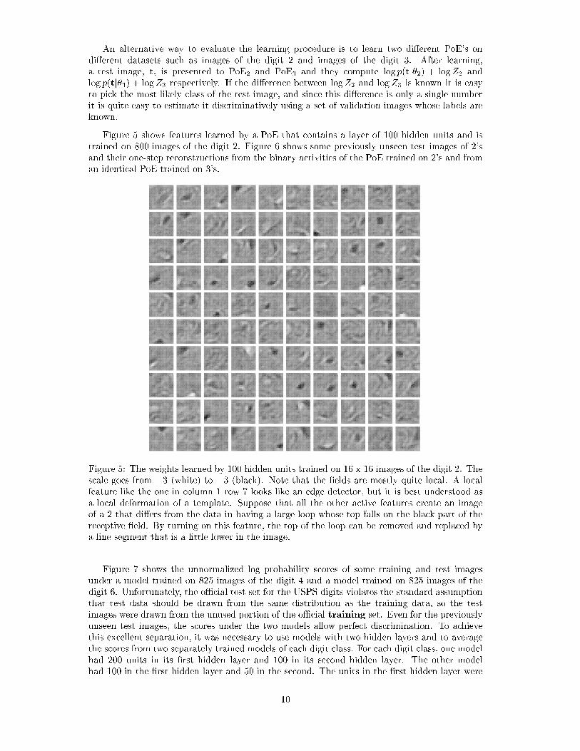
Figure 5 shows features learned by a PoE that contains a layer of 100 hidden units and istrained on 800 images of the digit 2. Figure 6 shows some previously unseen test images of 2'sand their one-step reconstructions from the binary activities of the PoE trained on 2's and froman identical PoE trained on 3's.

Figure 5: The weights learned by 100 hidden units trained on 16 x 16 images of the digit 2. Thescale goes from +3 (white) to �3 (black). Note that the �elds are mostly quite local. A localfeature like the one in column 1 row 7 looks like an edge detector, but it is best understood asa local deformation of a template. Suppose that all the other active features create an imageof a 2 that di�ers from the data in having a large loop whose top falls on the black part of thereceptive �eld. By turning on this feature, the top of the loop can be removed and replaced bya line segment that is a little lower in the image.

Figure 7 shows the unnormalized log probability scores of some training and test imagesunder a model trained on 825 images of the digit 4 and a model trained on 825 images of thedigit 6. Unfortunately, the oÆcial test set for the USPS digits violates the standard assumptionthat test data should be drawn from the same distribution as the training data, so the testimages were drawn from the unused portion of the oÆcial training set. Even for the previouslyunseen test images, the scores under the two models allow perfect discrimination. To achievethis excellent separation, it was necessary to use models with two hidden layers and to averagethe scores from two separately trained models of each digit class. For each digit class, one modelhad 200 units in its �rst hidden layer and 100 in its second hidden layer. The other modelhad 100 in the �rst hidden layer and 50 in the second. The units in the �rst hidden layer were

10

Figure 6: The center row is previously unseen images of 2's. The top row shows the pixelprobabilities when the image is reconstructed from the binary activities of 100 feature detectorsthat have been trained on 2's. The bottom row shows the reconstruction probabilities using 100feature detectors trained on 3's.

trained without regard to the second hidden layer. After training the �rst hidden layer, thesecond hidden layer was then trained using the probabilities of feature activation in the �rsthidden layer as the data.

a)

100 200 300 400 500 600 700 800 900100

200

300

400

500

600

700

800

900Log scores of both models on training data

Score under model−4

Sco

re u

nder

mod

el−

6

b)

100 200 300 400 500 600 700 800 900100

200

300

400

500

600

700

800

900Log scores under both models on test data

Score under model−4

Sco

re u

nder

mod

el−

6

Figure 7: a) The unnormalised log probability scores of the training images of the digits 4 and6 under the learned PoE's for 4 and 6. b) The log probability scores for previously unseen testimages of 4's and 6's. Note the good separation of the two classes.

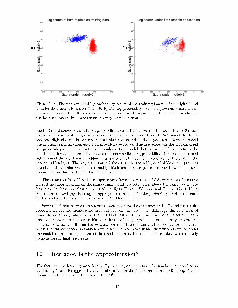
Figure 8 shows the unnormalized log probability scores for images of 7's and 9's which arethe most diÆcult classes to discriminate. Discrimination is not perfect on the test images, but itis encouraging that all of the errors are close to the decision boundary, so there are no con�dentmisclassi�cations.

9.1 Dealing with multiple classes

If there are 10 di�erent PoE's for the 10 digit classes it is slightly less obvious how to use the10 unnormalized scores of a test image for discrimination. One possibility is to use a validationset to train a logistic regression network that takes the unnormalized log probabilities given by

11

a)

100 200 300 400 500 600 700 800 900100

200

300

400

500

600

700

800

900Log scores of both models on training data

Score under model−7

Sco

re u

nder

mod

el−

9

b)

100 200 300 400 500 600 700 800 900100

200

300

400

500

600

700

800

900Log scores under both models on test data

Score under model−7

Sco

re u

nder

mod

el−

9

Figure 8: a) The unnormalised log probability scores of the training images of the digits 7 and9 under the learned PoE's for 7 and 9. b) The log probability scores for previously unseen testimages of 7's and 9's. Although the classes are not linearly separable, all the errors are close tothe best separating line, so there are no very con�dent errors.

the PoE's and converts them into a probability distribution across the 10 labels. Figure 9 showsthe weights in a logistic regression network that is trained after �tting 10 PoE models to the 10separate digit classes. In order to see whether the second hidden layers were providing usefuldiscriminative information, each PoE provided two scores. The �rst score was the unnormalizedlog probability of the pixel intensities under a PoE model that consisted of the units in the�rst hidden layer. The second score was the unnormalized log probability of the probabilities ofactivation of the �rst layer of hidden units under a PoE model that consisted of the units in thesecond hidden layer. The weights in �gure 9 show that the second layer of hidden units providesuseful additional information. Presumably this is because it captures the way in which featuresrepresented in the �rst hidden layer are correlated.

The error rate is 1.1% which compares very favorably with the 5.1% error rate of a simplenearest neighbor classi�er on the same training and test sets and is about the same as the verybest classi�er based on elastic models of the digits (Revow, Williams and Hinton, 1996). If 7%rejects are allowed (by choosing an appropriate threshold for the probability level of the mostprobable class), there are no errors on the 2750 test images.

Several di�erent network architectures were tried for the digit-speci�c PoE's and the resultsreported are for the architecture that did best on the test data. Although this is typical ofresearch on learning algorithms, the fact that test data was used for model selection meansthat the reported results are a biased estimate of the performance on genuinely unseen testimages. Mayraz and Hinton (in preparation) report good comparative results for the largerMNIST database at www.research.att.com/~yann/ocr/mnist and they were careful to do allthe model selection using subsets of the training data so that the oÆcial test data was used onlyto measure the �nal error rate.

10 How good is the approximation?

The fact that the learning procedure in Eq. 6 gives good results in the simulations described insections 4, 5, and 9 suggests that it is safe to ignore the �nal term in the RHS of Eq. 5 thatcomes from the change in the distribution Q

1.

12

Figure 9: The weights learned by doing multinomial logistic regression on the training data withthe labels as outputs and the unnormalised log probability scores from the trained, digit-speci�c,

PoE's as inputs. Each column corresponds to a digit class, starting with digit 1 The top row isthe biases for the classes. The next ten rows are the weights assigned to the scores that representthe log probability f the pixels under the model learned by the �rst hidden layer of each PoE.The last ten rows are the weights assigned to the scores that represent the log probabilities of theprobabilities on the �rst hidden layer under the the model earned by the second hidden layer.Note that although the weights in the last ten rows are smaller, they are still quite large whichshows that the scores from the second hidden layers provide useful, additional, discriminativeinformation.

To get an idea of the relative magnitude of the term that is being ignored, extensive simu-lations were performed using restricted Boltzmann machines with small numbers of visible andhidden units. By performing computations that are exponential in the number of hidden unitsand exponential in the number of visible units it is possible to compute the exact values of<sisj>Q0 and <sisj>Q1 . It is also possible to measure what happens to Q

0jjQ1 � Q1jjQ1

when the approximation in Eq. 10 is used to update the weights by an amount that is large

compared with the numerical precision of the machine but small compared with the curvatureof the contrastive divergence.

The RBM's used for these simulations had random training data and random weights. Theydid not have biases on the visible or hidden units. The main result can be summarized as follows:For an individual weight, the RHS of Eq. 10, summed over all training cases, occasionally di�ersin sign from the LHS. But for networks containing more than 2 units in each layer it is almostcertain that a parallel update of all the weights based on the RHS of Eq. 10 will improve thecontrastive divergence. In other words, when we average over the training data, the vector ofparameter updates given by the RHS is almost certain to have a positive cosine with the truegradient de�ned by the LHS. Figure 10a is a histogram of the improvements in the contrastivedivergence when Eq. 10 was used to perform one parallel weight update in each of a hundredthousand networks. The networks contained 8 visible and 4 hidden units and their weights werechosen from a Gaussian distribution with mean zero and standard deviation 20. With smallerweights or larger networks the approximation in Eq. 10 is even better.

Figure 10b shows that the learning procedure does not always improve the log likelihood ofthe training data, though it has a strong tendency to do so. Note that only 1000 networks were

13

a)

0 0.5 1 1.5

x 10−5

0

1000

2000

3000

4000

5000

6000

7000 Histogram of improvements in contrastive divergence

b)

−2 0 2 4 6 8 10

x 10−6

0

10

20

30

40

50

60 Histogram of improvements in data log likelihood

Figure 10: a) A histogram of the improvements in the contrastive divergence as a result of usingEq. 10 to perform one update of the weights in each of 105 networks. The expected values onthe RHS of Eq. 10 were computed exactly. The networks had 8 visible and 4 hidden units. Theinitial weights were randomly chosen from a Gaussian with mean 0 and standard deviation 20.The training data was chosen at random. b) The improvements in the log likelihood of the datafor 1000 networks chosen in exactly the same way as in �gure 10a. Note that the log likelihooddecreased in two cases. The changes in the log likelihood are the same as the changes in Q0jjQ1

but with a sign reversal.

used for this histogram.

Figure 11 compares the contributions to the gradient of the contrastive divergence made bythe RHS of Eq. 10 and by the term that is being ignored. For the vector of weight updatesgiven by Eq. 10 to make the contrastive divergence worse, the dots in �gure 11 would have tobe above the diagonal line, so it is clear that in these networks the approximation in Eq. 10is quite safe. Intuitively, we expect Q1 to lie between Q

0 and Q1 so when the parameters are

changed to move Q1 closer to Q0 the changes should also move Q1 towards Q0 and away fromthe previous position of Q1. So the ignored changes in Q

1 should cause an increase in Q1jjQ1

and thus an improvement in the contrastive divergence.

In an earlier version of this paper, the learning rule in Eq. 6 was interpreted as approximateoptimization of the contrastive log likelihood:

hlogQ1d iQ0 �logQ1

d̂

�Q1

Unfortunately, the contrastive log likelihood can achieve its maximum value of 0 by simplymaking all possible vectors in the data space equally probable. The contrastive divergence di�ersfrom the contrastive log likelihood by including the entropies of the distributions Q0 and Q1 (seeEq. 10) and so the high entropy of Q1 rules out the solution in which all possible data vectorsare equiprobable.

11 Other types of expert

Binary stochastic pixels are not unreasonable for modeling preprocessed images of handwrittendigits in which ink and background are represented as 1 and 0. In real images, however, thereis typically very high mutual information between the real-valued intensity of one pixel andthe real-valued intensities of its neighbors. This cannot be captured by models that use binarystochastic pixels because a binary pixel can never have more than 1 bit of mutual informationwith anything. It is possible to use \multinomial" pixels that have n discrete values. This is a

14

−0.5 0 0.5 1 1.5 2 2.5 3 3.5 4

−0.5

0

0.5

1

1.5

2

2.5

3

3.5

4

Modeled vs unmodeled effects

Figure 11: A scatterplot that shows the relative magnitudes of the modeled and unmodelede�ects of a parallel weight update on the contrastive divergence. The 100 networks used forthis �gure have 10 visible and 10 hidden units and their weights are drawn from a zero-meanGaussian with a standard deviation of 10. The horizontal axis shows

�Q

0jjQ1old

�Q1oldjjQ1

old

���

Q0jjQ1

new�Q

1oldjjQ1

new

�where old and new denote the distributions before and after the weight

update. This di�ers from the improvement in the contrastive divergence because it ignores thefact that changing the weights changes the distribution of the one-step reconstructions. Theignored term, Q1

oldjjQ1

new�Q1

newjjQ1

new, is plotted on the vertical axis. Points above the diagonal

line would correspond to cases in which the weight updates caused a decrease in the contrastivedivergence. Note that the unmodeled e�ects are almost always helpful rather than being incon ict with the modeled e�ects.

clumsy solution for images because it fails to capture the continuity and one-dimensionality ofpixel intensity, though it may be useful for other types of data. A better approach is to imaginereplicating each visible unit so that a pixel corresponds to a whole set of binary visible units thatall have identical weights to the hidden units. The number of active units in the set can thenapproximate a real-valued intensity. During reconstruction, the number of active units will bebinomially distributed and because all the replicas have the same weights, the single probabilitythat controls this binomial distribution only needs to be computed once. The same trick canbe used to allow replicated hidden units to approximate real-values using binomially distributedinteger states. A set of replicated units can be viewed as a computationallty cheap approximationto units whose weights actually di�er or it can be viewed as a stationary approximation to thebehaviour of a single unit over time in which case the number of active replicas is a �ring rate.

An alternative to replicating hidden units is to use \unifac" experts that each consist of amixture of a uniform distribution and a factor analyser with just one factor. Each expert hasa binary latent variable that speci�es whether to use the uniform or the factor analyser and areal-valued latent variable that speci�es the value of the factor (if it is being used). The factoranalyser has three sets of parameters: a vector of factor loadings which specify the directionof the factor in image space, a vector of means in image space, and a vector of variances inimage space5. Experts of this type have been explored in the context of directed acyclic graphs(Hinton, Sallans and Ghahramani, 1998) but they should work better in a product of experts.

An alternative to using a large number of relatively simple experts is to make each expert

5The last two sets of parameters are exactly equivalent to the parameters of a \unigauss" expert introduced

in section 4, so a \unigauss" expert can be considered to be a mixture of a uniform with a factor analyser that

has no factors.

15

as complicated as possible, whilst retaining the ability to compute the exact derivative of thelog likelihood of the data w.r.t. the parameters of an expert. In modeling static images, forexample, each expert could be a mixture of many axis-aligned Gaussians. Some experts mightfocus on one region of an image by using very high variances for pixels outside that region. Butso long as the regions modeled by di�erent experts overlap, it should be possible to avoid blockboundary artifacts.

11.1 Products of Hidden Markov Models

Hidden Markov Models (HMM's) are of great practical value in modeling sequences of discretesymbols or sequences of real-valued vectors because there is an eÆcient algorithm for updatingthe parameters of the HMM to improve the log likelihood of a set of observed sequences. HMM'sare, however, quite limited in their generative power because the only way that the portion of astring generated up to time t can constrain the portion of the string generated after time t is viathe discrete hidden state of the generator at time t. So if the �rst part of a string has, on average,n bits of mutual information with the rest of the string the HMM must have 2n hidden states toconvey this mutual information by its choice of hidden state. This exponential ineÆciency canbe overcome by using a product of HMM's as a generator. During generation, each HMM getsto pick a hidden state at each time so the mutual information between the past and the futurecan be linear in the number of HMM's. It is therefore exponentially more eÆcient to have manysmall HMM's than one big one. However, to apply the standard forward-backward algorithm toa product of HMM's it is necessary to take the cross-product of their state spaces which throwsaway the exponential win. For products of HMM's to be of practical signi�cance it is necessaryto �nd an eÆcient way to train them.

Andrew Brown (Brown and Hinton, in preparation) has shown that for a toy example involv-ing a product of four HMM's, the learning algorithm in Eq. 6 works well. The forward-backwardalgorithm is used to get the gradient of the log likelihood of an observed or reconstructed se-quence w.r.t. the parameters of an individual expert. The one-step reconstruction of a sequenceis generated as follows:

1. Given an observed sequence, use the forward-backward algorithm in each expert separatelyto calculate the posterior probability distribution over paths through the hidden states.

2. For each expert, stochastically select a hidden path from the posterior given the observedsequence.

3. At each time step, select an output symbol or output vector from the product of the output

distributions speci�ed by the selected hidden state of each HMM.

If more realistic products of HMM's can be trained successfully by minimizing the contrastivedivergence, they should be far better than single HMM's for many di�erent kinds of sequentialdata. Consider, for example, the HMM shown in �gure 12. This expert concisely captures anon-local regularity. A single HMM which must also model all the other regularities in strings ofEnglish words could not capture this regularity eÆciently because it could not a�ord to devoteit entire memory capacity to remembering whether the word \shut" had already occurred in thestring.

12 Discussion

There have been previous attempts to learn representations by adjusting parameters to cancelout the e�ects of brief iteration in a recurrent network (Hinton and McClelland, 1988; O'Reilly,1996, Seung, 1998), but these were not formulated using a stochastic generative model and anappropriate objective function.

16

<any word> shut <any word> the heck up

Figure 12: A Hidden Markov Model. The �rst and third nodes have output distributions thatare uniform across all words. If the �rst node has a high transition probability to itself, moststrings of English words are given the same low probability by this expert. Strings that containthe word \shut" followed directly or indirectly by the word \up" have higher probability underthis expert.

Minimizing contrastive divergence has an unexpected similarity to the learning algorithmproposed by Winston (1975). Winston's program compared arches made of blocks with \nearmisses" supplied by a teacher and it used the di�erences in its representations of the correct andincorrect arches to decide which aspects of its representation were relevant. By using a stochasticgenerative model we can dispense with the teacher, but it is still the di�erences between thereal data and the near misses generated by the model that drive the learning of the signi�cantfeatures.

12.1 Logarithmic opinion pools

The idea of combining the opinions of multiple di�erent expert models by using a weightedaverage in the log probability domain is far from new (Genest and Zidek, 1986; Heskes 1998),but research has focussed on how to �nd the best weights for combining experts that have alreadybeen learned or programmed separately (Berger, Della Pietra and Della Pietra, 1996) rather thantraining the experts cooperatively. The geometric mean of a set of probability distributions hasthe attractive property that its Kullback-Liebler divergence from the true distribution, P , issmaller than the average of the Kullback-Liebler divergences of the individual distributions, Q:

P jj�mQ

wmm

Z�Xm

wmP jjQm (12)

where the wm are non-negative and sum to 1, and Z =P

c�mQ

wmm

(c). When all of theindividual models are identical, Z = 1. Otherwise, Z is less than one and the di�erence betweenthe two sides of 12 is � logZ. This makes it clear that the bene�t of combining experts comesfrom the fact that they make logZ small by disagreeing on unobserved data.

It is tempting to augment PoE's by giving each expert, m, an additional adaptive parameter,

wm, that scales its log probabilities. However, this makes inference much more diÆcult (Yee-Whye Teh, personal communication). Consider, for example, an expert with wm = 100. Thisis equivalent to having 100 copies of an expert but with their latent states all tied together andthis tying a�ects the inference. So it is easier just to �x wm = 1 and allow the PoE learningalgorithm to determine the appropriate sharpness of the expert.

17

12.2 Comparison with directed acyclic graphical models

Inference in a PoE is trivial because the experts are individually tractable and the productformulation ensures that the hidden states of di�erent experts are conditionally independentgiven the data. This makes them relevant as models of biological perceptual systems, whichmust be able to do inference very rapidly. Alternative approaches based on directed acyclicgraphical models su�er from the \explaining away" phenomenon. When such graphical modelsare densely connected exact inference is intractable, so it is necessary to resort to clever butimplausibly slow iterative techniques for approximate inference (Saul and Jordan, 1998) or touse crude approximations that ignore explaining away during inference and rely on the learningalgorithm to �nd representations for which the shoddy inference technique is not too damaging(Hinton, Dayan, Frey and Neal, 1995).

Unfortunately, the ease of inference in PoE's is balanced by the diÆculty of generatingfantasy data from the model. This can be done trivially in one ancestral pass in a directedacyclic graphical model but requires an iterative procedure such as Gibbs sampling in a PoE. If,however, Eq. 6 is used for learning, the diÆculty of generating samples from the model is not amajor problem.

In addition to the ease of inference that results from the conditional independence of theexperts given the data, PoE's have a more subtle advantage over generative models that workby �rst choosing values for the latent variables and then generating a data vector from theselatent values. If such a model has a single hidden layer and the latent variables have independentprior distributions, there will be a strong tendency for the posterior values of the latent variablesto be approximately marginally independent after the model has been �tted to data6. For thisreason, there has been little success with attempts to learn such generative models one hiddenlayer at a time in a greedy, bottom-up way. With PoE's, however, even though the experts haveindependent priors the latent variables in di�erent experts will be marginally dependent: Theycan have high mutual information even for fantasy data generated by the PoE itself. So afterthe �rst hidden layer has been learned greedily there may still be lots of statistical structure inthe latent variables for the second hidden layer to capture.

The most attractive property of a set of orthogonal basis functions is that it is possible to

compute the coeÆcient on each basis function separately without worrying about the coeÆcientson other basis functions. A PoE retains this attractive property whilst allowing non-orthogonalexperts and a non-linear generative model.

PoE's provide an eÆcient instantiation of the old psychological idea of analysis-by-synthesis.This idea never worked properly because the generative models were not selected to make theanalysis easy. In a PoE, it is diÆcult to generate data from the generative model, but, given themodel, it is easy to compute how any given data vector might have been generated and, as wehave seen, it is relatively easy to learn the parameters of the generative model.

Acknowledgements

This research was funded by the Gatsby Foundation. Thanks to Zoubin Ghahramani, David MacKay,

David Lowe, Yee-Whye Teh, Guy Mayraz, Andy Brown, and other members of the Gatsby unit for

helpful discussions and to Peter Dayan for improving the manuscript and disproving some expensive

speculations.

6This is easy to understand from a coding perspective in which the data is communicated by �rst specifying

the states of the latent variables under an independent prior and then specifying the data given the latent states.

If the latent states are not marginally independent this coding scheme is ineÆcient, so pressure towards coding

eÆciency creates pressure towards independence.

18

References

Berger, A., Della Pietra, S. and Della Pietra, V. (1996) A Maximum Entropy Approach toNatural Language Processing. Computational Linguistics, 22.

Freund, Y. and Haussler, D. (1992) Unsupervised learning of distributions on binary vectorsusing two layer networks. Advances in Neural Information Processing Systems 4. J. E. Moody,S. J. Hanson and R. P. Lippmann (Eds.), Morgan Kaufmann: San Mateo, CA.

Genest, C. & Zidek, J. V. (1986) Combining probability distributions: A critique and anannotated bibliography. Statistical Science 1, 114-148.

Heskes, T. (1998) Bias/Variance decompositions for likelihood-based estimators. Neural

Computation 10, 1425-1433.

Hinton, G., Dayan, P., Frey, B. & Neal, R. (1995) The wake-sleep algorithm for self-organizingneural networks. Science, 268, 1158-1161.

Hinton, G. E. Sallans, B. and Ghahramani, Z. (1998) Hierarchical Communities of Experts.In M. I. Jordan (Ed.) Learning in Graphical Models. Kluwer Academic Press.

Hinton, G. E. & McClelland, J. L. (1988) Learning representations by recirculation. InD. Z. Anderson, editor, Neural Information Processing Systems, 358{366, American Institute ofPhysics: New York.

Hinton, G. E. & Sejnowski, T. J. (1986) Learning and relearning in Boltzmann machines. InRumelhart, D. E. and McClelland, J. L., editors, Parallel Distributed Processing: Explorations

in the Microstructure of Cognition. Volume 1: Foundations, MIT Press

O'Reilly, R. C. (1996) Biologically Plausible Error-Driven Learning Using Local ActivationDi�erences: The Generalized Recirculation Algorithm. /it Neural Computation, /bf 8, 895-938.

Revow, M., Williams, C. K. I. and Hinton, G. E. (1996) Using Generative Models for Hand-written Digit Recognition. IEEE Transactions on Pattern Analysis and Machine Intelligence,18, 592-606.

Saul, L. K., Jaakkola, T. & Jordan, M. I. (1996) Mean �eld theory for sigmoid belief networks.Journal of Arti�cial Intelligence Research, 4 61-76.

Seung, H. S. (1998) Learning continuous attractors in a recurrent net. Advances in Neural

Information Processing Systems 10. M. I. Jordan, M. J. Kearns, and S. A. Solla (Eds.) MITPress, Cambridge Mass.

Smolensky, P. (1986) Information processing in dynamical systems: Foundations of harmonytheory. In Rumelhart, D. E. and McClelland, J. L., editors, Parallel Distributed Processing:

Explorations in the Microstructure of Cognition. Volume 1: Foundations, MIT Press

Winston, P. H. (1975) Learning structural descriptions from examples. In Winston, P. H.(Ed.) The Psychology of Computer Vision, McGraw-Hill Book Company, New York.

19