TRAINING MANUAL For Institutional Stakeholders
64
Small-scale, low-cost, environment friendly irrigation schemes: sites selection and preparation of full work tender dossier EuropeAid/137393/DH/SER/MK Component 2: Support for stakeholders involved in planning and implementation of the irrigation sector policy TRAINING MANUAL For Institutional Stakeholders SUBJECT: • Software applications for irrigation • CROPWAT, CLIMWAT, SIRMOD Date: 27 September 2018 This project is funded by the European Union A project implemented by:
Transcript of TRAINING MANUAL For Institutional Stakeholders

Small-scale, low-cost, environment friendly irrigation schemes:
sites selection and preparation of full work tender dossier EuropeAid/137393/DH/SER/MK
Component 2: Support for stakeholders involved in planning and implementation of the irrigation sector policy
TRAINING MANUAL For Institutional Stakeholders SUBJECT:
• Software applications for irrigation
• CROPWAT, CLIMWAT, SIRMOD
Date: 27 September 2018
This project is funded
by the European Union
A project implemented by:

This project is funded by the European Union
Small Scale Irrigation Projects EuropeAid/137393/DH/SER/MK
Page 2| 64
Table of Contents
1 EXECUTIVE SUMMARY ......................................................................................... 3
2 IRRIGATION DATABASES AND SOFTWARE ............................................................ 4 2.1 AQUASTAT ................................................................................................................................ 4
2.2 AQUACROP ............................................................................................................................... 4
2.3 AQUAMAPS ............................................................................................................................... 5
2.4 CROP WATER INFORMATION ................................................................................................... 5
2.5 CROPWAT ................................................................................................................................. 5
2.6 CLIMWAT .................................................................................................................................. 6
2.7 OTHER FAO DATABASES AND SOFTWARE ................................................................................ 7
2.8 USDA NRCS SOFTWARE: ........................................................................................................... 7
2.1 UTAH STATE UNIVERSITY SOFTWARE: ...................................................................................... 9
2.2 IRRIGATION SYSTEM MANAGEMENT AND CONTROL SYSTEMSE ............................................. 9
3 CROPWAT .......................................................................................................... 10 3.1 Introduction ............................................................................................................................ 10
3.2 Input ....................................................................................................................................... 10
3.3 Output .................................................................................................................................... 12
3.4 Calculation methods ............................................................................................................... 12
3.5 The Program Structure ........................................................................................................... 19
4 DESIGN AND EVALUATION OF SURFACE IRRIGATION SYSTEMS: SIRMOD MODEL (WALKER, 2003) ................................................................................................. 39
4.1 SURFACE IRRIGATION SYSTEM DESIGN .................................................................................. 39
4.2 PROGRAM STRUCTURE ........................................................................................................... 41
4.3 THE DESIGN PROCESS ............................................................................................................. 47
4.4 THE EVALUATION PROCESS .................................................................................................... 47
5 IRRIGATION SYSTEM MANAGEMENT AND CONTROL SOFTWARE/SYSTEMS ......... 51
6 BIBLIOGRAPHY ................................................................................................... 55
7 ANNEXES ............................................................................................................ 56 7.1 ANNEX I: Evaluation of irrigation performance ...................................................................... 56
This project is funded by the European Union
Small Scale Irrigation Projects EuropeAid/137393/DH/SER/MK
Page 3| 64
1 EXECUTIVE SUMMARY
According to the Terms of Reference (ToR), the objective of Component 2: “Support for stakeholders
involved in planning and implementation of the irrigation sector policy” is to provide capacity building
of stakeholders in irrigation management, targeting the Water Management Directorate (WMD) at
the Ministry of Agriculture, Forestry and Water Economy (MAFWE), and the Joint Stock Company for
Water Management (JSCWM) and farmer’s groups at the selected sites.
The support to the institutional stakeholders (WMD at MAFWE and JSCWM) should
1) provide clarifications and transfer necessary knowledge about practical application of the
selected standardised methodology used to prepare the outputs under Component 1
2) support to successfully carry out the ongoing policy to transfer the responsibility for water
management to water users
This support will be provided through the following trainings subjects:
1) Methodology used for Pre-feasibility studies
2) Strategy to transfer/share water management to irrigation water users (Irrigation
Management Transfer - IMT) (Workshop)
3) System Irrigation Management
4) On farm irrigation water management
5) Software applications for irrigation: CROPWAT, CLIMWAT, SIRMOD, etc.
6) Methodology to be used for feasibility studies
7) Basin Water Resources Management
8) Agriculture economics.
Capacity needs assessment
During the trainings, a capacity needs assessment questionnaire will identify the following subjects of
interest for future training. The subjects of interest up to now are:
9) Participatory methods
10) Methodology to be used for Main Designs
11) Formation of water users’ associations (WUAs)
12) Workshop(s) on water tariff methodology.
13) Tender Dossier Preparation (following latest EU PRAG rules)
14) Application procedures to different donors / multilateral and bilateral org.

This project is funded by the European Union
Small Scale Irrigation Projects EuropeAid/137393/DH/SER/MK
Page 4| 64
2 IRRIGATION DATABASES AND SOFTWARE
The Food and Agriculture Organization of the United Nations (FAO) hosts state-of-the-art databases and software to monitor and manage the many variables required to ensure food security while minimizing environmental impacts. All FAO’s standalone software models and other tools can be downloaded free, for use directly in the field or to assist in research projects. (http://www.fao.org/land-water/databases-and-software/en/) Key databases and software models include:
2.1 AQUASTAT
AQUASTAT is FAO’s global water information system. It collects, analyses and disseminates data and information by country, by region and for the world. Its aim is to provide users interested in global, regional and national analyses with comprehensive information related to water resources, water uses and agricultural water management across the world. Among the information available: main country database; datasets; country profiles and fact sheets; regional overviews; transboundary river basin profiles; water resources; georeferenced dams database; water uses; wastewater; irrigation water use and irrigated crop calendars; global map of irrigation areas by source of water; water and gender; water-related country-level institutional framework; wide variety of tables, maps and spatial data; visualizations and infographics; a multilingual glossary; water-related institutions database; climate information tool; information for the media; a wide range of publications; key water indicator portal; UN-Water country briefs; Sustainable Development Goal indicator 6.4 on water stress and water use efficiency. The entire AQUASTAT website is available in three languages: English, French and Spanish.
2.2 AQUACROP
AquaCrop is a crop growth model developed by the Land and Water Division of FAO to simulate yield response to water of herbaceous crops, and is particularly suited to address conditions where water is a key limiting factor in crop production. AquaCrop uses only a relatively small number of explicit parameters and mostly-intuitive input-variables requiring simple methods for their determination. On the other hand, the calculation procedures are grounded on basic and often complex biophysical processes to guarantee an accurate simulation of the response of the crop in the plant-soil system. AquaCrop uses the original 1979 FAO 33 equation and evolves from it by calculating the crop biomass, based on the amount of water transpired, and the crop yield as the proportion of biomass that goes into the harvestable parts. Also separates of the non-productive consumption of water (soil evaporation) from the productive consumption of water (transpiration). The timescale is shortened from seasonal to daily, and the model allows for the assessment of responses under different climate change scenarios in terms of altered water and temperature regimes and elevated carbon dioxide concentration in the atmosphere. For more information on AquaCrop, visit www.fao.org/aquacrop

This project is funded by the European Union
Small Scale Irrigation Projects EuropeAid/137393/DH/SER/MK
Page 5| 64
2.3 AQUAMAPS
AquaMaps is the FAO global online spatial database on water and agriculture. It makes accessible through a simple interface regional and global spatial datasets on water resources and water management considered as a standard information resource, produced by FAO or by external data providers. AquaMaps is complementary to AQUASTAT, FAO's Information System on Water and Agriculture. While AQUASTAT focuses on collecting mainly statistical data and qualitative information on
(sub)country level, AquaMaps concentrates on geographical information AquaMaps builds on the FAO GeoNetwork data catalogue, from which it retrieves a thematic collection of layers, data and metadata, allowing users to query, explore, and download spatial data in commonly used GIS format. The collection of dataset is organized by themes:
• River and water bodies: regional hydrographic networks derived from Hydrosheds
• Irrigation and infrastructures: area equipped for irrigation, dams
• Hydrological basins: global and regional layers of hydrological basins derived from Hydrosheds
• Climate: Monthly grids of precipitation and reference evapotranspiration
• Models: output grid of FAO global soil water balance model (GlobWat), including modeled actual evapotranspiration, runoff and infiltration
• Analyses: examples of global analyses performed on the basis of the above mentioned dataset.
2.4 CROP WATER INFORMATION
Crop water information presents information about individual crops, their crop water requirement, yield response to water; and bibliographic database on crop water productivity.
2.5 CROPWAT
CROPWAT 8.0 for Windows is a computer program for the calculation of crop water requirements and irrigation requirements based on soil, climate and crop data. In addition, the program allows the development of irrigation schedules for different management conditions and the calculation of scheme water supply for varying crop patterns. CROPWAT 8.0 can also be used to evaluate farmers’ irrigation practices and to estimate crop performance under both rainfed and irrigated conditions.

This project is funded by the European Union
Small Scale Irrigation Projects EuropeAid/137393/DH/SER/MK
Page 6| 64
All calculation procedures used in CROPWAT 8.0 are based on the two FAO publications of the Irrigation and Drainage Series, namely, No. 56 "Crop Evapotranspiration - Guidelines for computing crop water requirements” and No. 33 titled "Yield response to water". As a starting point, and only to be used when local data are not available, CROPWAT 8.0 includes standard crop and soil data. When local data are available, these data files can be easily modified or new ones can be created. Likewise, if local climatic data are not available, these can be obtained for over 5,000 stations worldwide from CLIMWAT, the associated climatic database. The development of irrigation schedules in CROPWAT 8.0 is based on a daily soil-water balance using various user-defined options for water supply and irrigation management conditions. Scheme water supply is calculated according to the cropping pattern defined by the user, which can include up to 20 crops. CROPWAT 8.0 is a Windows program based on the previous DOS versions. Apart from a completely redesigned user interface, CROPWAT 8.0 for Windows includes a host of updated and new features, including the possibility to estimate climatic data in the absence of measured values
2.6 CLIMWAT
CLIMWAT is a climatic database to be used in combination with the computer program CROPWAT. and allows the calculation of crop water requirements, irrigation supply and irrigation scheduling for various crops for a range of climatological stations worldwide.
CLIMWAT 2.0 offers observed agroclimatic data of over 5000 stations worldwide distributed as shown in the map. CLIMWAT provides long-term monthly mean values of seven climatic parameters, namely:
• Mean daily maximum temperature in °C
• Mean daily minimum temperature in °C
• Mean relative humidity in %
• Mean wind speed in km/day
• Mean sunshine hours per day
• Mean solar radiation in MJ/m2/day
• Monthly rainfall in mm/month
• Monthly effective rainfall in mm/month
• Reference evapotranspiration calculated with the Penman-Monteith method in mm/day.
The data can be extracted for a single or multiple stations in the format suitable for their use in CROPWAT. Two files are created for each selected station. The first file contains long-term monthly rainfall data [mm/month]. Additionally, effective rainfall is also included calculated and included in the same file. The second file consists of long-term monthly averages for the seven climatic parameters, mentioned above. This file also contains the coordinates and altitude of the location.
All variables, except potential evapotranspiration, are direct observations or conversions of observations. Original data coming from a large number of meteorological stations as included in CLIMWAT, could not be uniform. For example, humidity and radiation can be expressed through different variables. (relative humidity, dew point temperature or water vapour pressure). The same

This project is funded by the European Union
Small Scale Irrigation Projects EuropeAid/137393/DH/SER/MK
Page 7| 64
problem arises with radiation. As a result, the provided relative humidity and sunshine hours are often deduced from observations of vapour pressure and radiation, even if the former are observed. The procedure, however, ensures that the different expressions are coherent.
In compiling the data, an effort was made to cover the period 1971 - 2000, but when data for this period were not available, any recent series that ends after 1975 and that has at least 15 years of data have been included. Some of the series are "broken", but they nevertheless have at least 15 years of data (e.g. 1961-70 and 1992-2000).
2.7 OTHER FAO DATABASES AND SOFTWARE
In the web site of the Land and Water Division of FAO. (http://www.fao.org/land-water/databases-and-software/en/) the other following databases and software can be found:
• GAEZ: Global Agro-Ecological Zones
• Harmonized World Soil Database v 1.2: 15 000 soil mapping units combining existing regional and national updates of soil information worldwide
• ETo calculator: is a software to calculate ETo according to FAO standards
• GLADIS Global Land Degradation Information System
• WATERLEX is a legislative database contains an analysis of the legal framework governing water resources in a large number of countries.
2.8 USDA NRCS SOFTWARE:
In the web site of the United States Department of Agriculture, Natural Resources Conservations Service another software related with irrigation can be found., for example:
(https://www.nrcs.usda.gov/wps/portal/nrcs/detailfull/national/ndcsmc/?cid=stelprdb1042198)
AgPipe 1.1 Beta: is for use in the design of irrigation and livestock pipe systems. The hydraulic pipeline program designs tanks, evaluates surge/water hammer, pipe deflection and the preliminary identification of pipeline valve suggestions, such as air vents.
Animal Waste Management is a planning/design tool for animal feeding operations that can be used to estimate the production of manure, bedding, process water and determine the size of storage/treatment facilities.
CPED 4.0.06 Center Pivot Evaluation and Design is a tool for the assessment of center pivot performance.
CropFlex 2005: CropFlex is a management system for irrigated crops. The goal of CropFlex is to provide irrigation and fertility management advice to assist farmers in maintaining or increasing yields while minimizing the potential of leaching nitrates.

This project is funded by the European Union
Small Scale Irrigation Projects EuropeAid/137393/DH/SER/MK
Page 8| 64
DrainMod 6.1, Build 103: Drain Modification simulates the hydrology of poorly drained, high water table soils on an hour-by-hour, day-by-day basis for long periods of climatological record (e.g. 40 years). The model predicts the effects of drainage and associated water management practices.
FIRI 1.2 REL 2: Field Irrigation Rating Index approximates or quantifies approximate water conservation through changes made to irrigation systems or through management.
IWRPM 1: Irrigation Water Requirements - Penman Monteith (IWRPM) is a crop consumptive use program using the Penman-Monteith equation for evapotranspiration developed specifically for NRCS use in development of Consumptive Use Tables for the NRCS Irrigation Guide.
ND-Drain 1.0.1 ND-Drain determines lateral effect of drains in close proximity to wetlands.
Phaucet 8.2.20 PHAUCET is a tool to design and evaluate furrow irrigation systems.
RUSLE2 2.5.2.11: The Revised Universal Soil Loss Equation (RUSLE2) is the NRCS tool to predict sheet and rill erosion from rainfall or water, utilizing the soil condition index, the soil tillage intensity rating, and energy requirements for the planned crop system.
SITES 2005 1.8: Rainfall runoff for hydraulically proportioning the principal spillway and auxiliary spillway of a dam.
SPAW 6.02.75 Soil, Plant, Atmosphere, and Water is a water budgeting tool for farm fields, ponds and inundated wetlands.
Structural Design 1.1.0: Software for the following NRCS structural design procedures:
• TR-42 – Single Cell Rectangular Conduits Criteria and Procedures for Structural Design
• TR-45 – Twin Cell Rectangular Conduits-Criteria and Procedures for Structural Design
• TR-50 – Design of Rectangular Structural Channels
• TR-54 – Structural Design of SAF Stilling Basins
• TR-54-1 – Structural Design of SAF Stilling Basins, Revised Wingwall Design, Amendment 1
• TR-63 – Structural Design of Monolithic Straight Drop Spillways
TR-19 RESOP RESOP is a tool to determine water storage requirements to meet supply and demand. A water budget calculator.
WinFlume 1.06.0006: A Windows-based computer program used to design and calibrate longthroated flume and broad-crested weir flow measurement structures. The software was developed through the cooperative efforts of the Bureau of Reclamation, the Agricultural Research Service, and the International Institute for Land Reclamation & Improvement.
WinPond 1.7 WinPond is a tool used for the hydrologic and hydraulic design of small earthen ponds (NHCP-378).
Win-PST 3.1 Base: WIN-PST is a pesticide environmental risk screening tool that NRCS field office conservationists, extension agents, crop consultants, pesticide dealers and producers can use to evaluate the potential for pesticides to move with water and eroded soil/organic matter and affect non-target organisms.

This project is funded by the European Union
Small Scale Irrigation Projects EuropeAid/137393/DH/SER/MK
Page 9| 64
WinSRFR 4.1.3 Surface irrigation system modeling.
WinTR-20 is a single event watershed scale runoff and routing model. It computes direct runoff and develops hydrographs resulting from any synthetic or natural rainstorm. Developed hydrographs are routed through stream and valley reaches as well as through reservoirs. Data requirements include rainfall data, watershed data, and cross section data.
Win TR-55 1.00.10: Small Watershed Hydrology. WinTR-55 is a tool for urban hydrology forsmall watersheds.
2.1 UTAH STATE UNIVERSITY SOFTWARE:
SIRMOD is a comprehensive software package for simulating the hydraulics of surface irrigation systems at the field level, selecting a combination of sizing and operational parameters that maximize application efficiency and a two-point solution of the “inverse” problem allowing the computation of infiltration parameters from the input of advance data. It was not possible to get a link where to obtain the SIRMOD program, but it was possible to obtain the SURFACE model from USDA NRCS. SURFACE
model and SIRMOD model are the same. The last button in top of the model switch surface model to SIRMOD model.
2.2 IRRIGATION SYSTEM MANAGEMENT AND CONTROL SYSTEMSE
SIMIS:
The Scheme Irrigation Management Information System (SIMIS) program has been developed by FAO with the aim of facilitating the operational activities in irrigation networks and improving integral administration of water. The main menu shows four options: Projects, Project Support, Project Management and Configuration. The Project Support module includes: climate, crops, soils, physical infrastructure, land tenure, machinery and implements, and staff. The management tools of the projects are: agricultural activities, crop water requirement, seasonal irrigation planning, irrigation scheduling, water consumption, accounting, operation and maintenance activities and costs, and water fees.
I was not able to get access to this software. it seems FAO is not providing and promoting it any more.
INTAGES
Intagés is an “Irrigation Control System” that provides remote full access and operational control of an installation from anywhere, developed by EPTISA. There are many of this commercial irrigation management systems. It is not just a software, but a system that includes sensors, valves and other controlers that allows remote control of the irrigation infrastructure. Intages is described as one of the possible options available in the market.

This project is funded by the European Union
Small Scale Irrigation Projects EuropeAid/137393/DH/SER/MK
Page 10| 64
3 CROPWAT
3.1 INTRODUCTION
CROPWAT is a computer program that allows To calculate:
• Reference evapotranspiration • Crop water requirements • Irrigation requirements • Scheme water supply
To develop Irrigation schedules under various management conditions To estimate: Rainfed production and drought effects
3.2 INPUT
Calculations of the crop water requirements and irrigation requirements are carried out with inputs of climatic, crop and soil data. For the estimation crop water requirements (CWR) the model requires: a) Reference Crop Evapotranspiration (Eto) values measured or calculated using the FAO Penman-Montieth equation based on decade/monthly climatic data:
• minimum and maximum air temperature,
• relative humidity,
• sunshine duration and
• windspeed; b) Rainfall data (daily/decade/monthly data); monthly rainfall is divided into a number of rain storm each month; c) A Cropping Pattern consisting of the planting date, crop coefficient data files (including Kc values, stage days, root depth, depletion fraction) and the area planted (0-100% of the total area); a set of typical crop coefficient data files are provided in the program.
In addition, for Irrigation Scheduling the model requires information on: d) Soil type: maximum soil infiltration rate, maximum rooting depth, total available soil moisture and initial soil moisture depletion (% of total available moisture);

This project is funded by the European Union
Small Scale Irrigation Projects EuropeAid/137393/DH/SER/MK
Page 11| 64
Soil texture: it indicates the relative content of particles of various
sizes, such as sand, silt and clay in the soil. The texture of a soil is
permanent, the farmer is unable to modify or change it.
Table 3-1 Denomination of soil textures
The infiltration rate of a soil is the velocity at which water can seep
into it. It is commonly measured by the depth (in mm) of the water
layer that the soil can absorb in an hour.
Table 3-2 Typical values for soils infiltration rates
Maximum rooting depth: The root depth of a crop influences the
maximum amount of water which can be stored in the root zone
Table 3-3 Approximate root depth of the major field crops
Total available soil moisture and initial soil moisture depletion (% of total available moisture)
Table 3-4 Available water content of different soils
e) Scheduling Criteria – several options can be selected regarding the calculation of application timing and application depth (e.g. 80 mm every 14 days, or irrigate to return the soil back to field capacity when all the easily available moisture has been used).
Expression used by the farmer
Expression used in literature
light sandy coarse
medium loamy medium
heavy clayey fine
Low infiltration rate less than 15 mm/hour
medium infiltration rate 15 to 50 mm/hour
high infiltration rate more than 50 mm/hour
Soil Available water content in mm water depth per m soil depth (mm/m) or (%)
sand 25 to 100 mm/m (2,5 to 10%)
loam 100 to 175 mm/m (10 to 17,5%)
clay 175 to 250 mm/m (17,5 to 25%)

This project is funded by the European Union
Small Scale Irrigation Projects EuropeAid/137393/DH/SER/MK
Page 12| 64
3.3 OUTPUT
Once all the data is entered, CropWat automatically calculates the results as tables or plotted in graphs. The time step of the results can be any convenient time step: daily, weekly, decade or monthly. The output parameters for each crop in the cropping pattern are: -reference crop evapotranspiration – Eto (mm/period); -crop Kc - average values of crop coefficient for each time step; -effective rain (mm/period) - the amount of water that enters the soil; -crop water requirements – CWR or Etm (mm/period); -irrigation requirements –IWR (mm/period); -total available moisture –TAM (mm); -readily available moisture – RAM (mm); -actual crop evapotranspiration – Etc (mm); -ratio of actual crop evapotranspiration to the maximum crop evapotranspiration - Etc/Etm (%); -daily soil moisture deficit (mm); -irrigation interval (days) & irrigation depth applied (mm); -lost irrigation (mm)– irrigation water that is not stored in the soil (i.e. either surface runoff or percolation); -estimated yields reduction due to crop stress (when Etc/Etm falls below 100%).
3.4 CALCULATION METHODS
3.4.1 ETO (ALLEN ET AL, 1998)
A large number of more or less empirical methods have been developed over the last half of the previous century. These were often subject to rigorous local calibrations and proved to have limited global validity. In the FAO Irrigation and Drainage Paper No. 24 'Crop water requirements' (1977), four methods were presented to calculate the reference crop evapotranspiration (ETo):
• Blaney-Criddle: for areas where available climatic data cover air temperature data only The calculation procedure is simple.
• Radiation: suggested for areas where available climatic data include measured air temperature and sunshine, cloudiness or radiation, but not measured wind speed and air humidity.
• Pan evaporation: It was expected this method would give acceptable estimates, depending on the location of the pan. The installation of a pan and data collection was needed in every location.
• Modified Penman: was considered to offer the best results with minimum possible error in relation to a living grass reference crop.
Numerous researchers analyzed the performance of the four methods for different locations. A major study was undertaken under the auspices of the Committee on Irrigation Water Requirements of the American Society of Civil Engineers (ASCE), and the European Community commissioned to a consortium of European research institutes the evaluation of various evapotranspiration methods. The comparative studies may be summarized as follows:
• Temperature methods (including Blaney-Criddle) remain empirical and require local calibration in order to achieve satisfactory results. A possible exception is the 1985

This project is funded by the European Union
Small Scale Irrigation Projects EuropeAid/137393/DH/SER/MK
Page 13| 64
Hargreaves’ method which has shown reasonable ETo results with a global validity. (information about this method can be obtained from Allen et al, 1998)
• The radiation methods show good results in humid climates where the aerodynamic term is relatively small, but performance in arid conditions is erratic and tends to underestimate evapotranspiration.
• Pan evapotranspiration methods clearly reflect the shortcomings of predicting crop evapotranspiration from open water evaporation. The methods are susceptible to the microclimatic conditions under which the pans are operating and the rigor of station maintenance. Their performance proves erratic.
• The Penman methods may require local calibration of the wind function to achieve satisfactory results. was frequently found to overestimate ETo, even up to 20% for low evaporative conditions
• The relatively accurate and consistent performance of the Penman-Monteith approach in both arid and humid climates has been indicated in both the ASCE and European studies.
A consultation of experts and researchers was organized by FAO in May 1990, in collaboration with the International Commission for Irrigation and Drainage and with the World Meteorological Organization, to review the FAO methodologies on crop water requirements and to advise on the revision and update of procedures. The panel of experts recommended the adoption of the Penman-Monteith combination method as a new standard for reference evapotranspiration. The method provides values more consistent with actual crop water use data worldwide. The assessment of the reference evapotranspiration ETo with the Penman-Monteith method is developed in Chapter 4. The calculation requires mean daily, ten-day or monthly maximum and minimum air temperature (Tmax and Tmin), actual vapour pressure (ea), net radiation (Rn) and wind speed measured at 2 m (u2). If some of the required weather data are missing or cannot be calculated, it is strongly recommended that the user estimate the missing climatic data with one of the procedures described in Allen et al, 1998, and use the FAO Penman-Monteith method for the calculation of ETo. The use of an alternative ETo calculation procedure, requiring only limited meteorological parameters, is less recommended. CROPWAT can estimate climatic data based in Temperature data and location, as is described more ahead in this training material. Penman equation: The constituents of the original Penman equation is described described
to understand the logic of the equation:
A is the amount of energy for evapotranspiration coming from the sunshine and the temperature of the air. It depends on the length of the day, the strength of the sunshine and the albedo of the crop
B is the amount of energy radiated back from the crop (mainly at night). This reduces the amount
Albedo [α]: is the fraction of the solar radiation reflected by the surface. It is highly variable for different surfaces and for the angle of incidence or slope of the surface: 0.95 for freshly fallen snow, 0.05 for a wet bare soil, 0.20-0.25 for a green vegetation cover. For the grass reference crop, α is assumed to have a value of 0.23

This project is funded by the European Union
Small Scale Irrigation Projects EuropeAid/137393/DH/SER/MK
Page 14| 64
of energy available to evaporate water. It depends on the air temperature, how cloudy it is and how humid the air is.
( A – B ): in the energy balance, the difference between the incoming and outgoing solar radiation ( Δ/γ ) is a dimensionless weighting factor that ensures that the other pans of the equation are correctly weighted before they are combined. A depends on the air temperature, but Δ is a constant. Ea is an term adds in the drying effect of the wind. It depends on the wind speed and the humidity of the air.
Penman-Monteich equation: Monteich incorporated:
• G: losses from soil surface • two other resistance coefficients (ra and rs) are used to
describe how the plant controls the delivery of water from the leaf into the atmosphere.
Aerodynamic resistance (ra): models the transfer of heat and water vapour from the evaporating surface into the air above the canopy. (Bulk) surface resistance (rs): describes the resistance of vapour flow through the transpiring crop and evaporating soil surface. (both are difficult to measure) FAO Penman-Monteich equation: FAO adopted the Penman-Monteich equation but introduced simplifications to enable it to be of practical use to irrigation specialists. The simplifications were to define a theoretical crop known as the Reference Crop: A short green crop 12cm high with a fixed canopy resistance of 90 sm-', albedo of 0.23., actively growing, completely shading the soil and not short of water. This definition removes the complexity of ra and rs, by assuming no water stress and a uniform leaf area. A set of Crop Coefficients Kc are needed for it to be used with other crops
Ea (A-B)

This project is funded by the European Union
Small Scale Irrigation Projects EuropeAid/137393/DH/SER/MK
Page 15| 64
CROPWAT uses standard climatological records of solar radiation (sunshine), air temperature, humidity and wind speed. To ensure the integrity of computations, the weather measurements should be made at 2 m (or converted to that height) above an extensive surface of green grass, shading the ground and not short of water. The location (altitude above sea level (m) and latitude (degrees north or south)) is needed to adjust some weather parameters for the local average value of atmospheric pressure (a function of the site elevation above mean sea level) and to compute extraterrestrial radiation (Ra) and, in some cases, daylight hours (N). In the calculation procedures for Ra and N, the latitude is expressed in radian (i.e., decimal degrees/180). Apart from the site location, the FAO Penman-Monteith equation requires air temperature, humidity, radiation and wind speed data for performing ten-day or monthly calculations. It is important to verify the units in which the weather data are reported. In CROPWAT, the values of decade or monthly Reference Crop Evapotranspiration (Eto) are converted into daily values using four distribution models (the default is a polynomial curve fitting).
3.4.2 CROP WATER REQUIREMENTS
The model calculates the Crop Water using the equation: CWR=Eto*Kc*area planted. This means that the peak CWR in mm/day can be less than the peak Eto value when less than 100% of the area is planted in the cropping pattern. The average values of crop coefficient for each time step are estimated by linear interpolation between the Kc values for each crop development stage. The “Crop Kc” values are calculated as Kc*Crop Area, so if the crop covers only 50% of the area, the “Crop Kc” values will be half of the Kc values in the crop coefficient data file.
3.4.3 EFFECTIVE RAINFALL
For crop water requirements and scheduling purposes, the monthly total rainfall has to be distributed into equivalent daily values. CropWat for Windows does this in two steps. First the rainfall from month to month is smoothed into a continuous curve (the default curve is a polynomial curve, but can be selected other smoothing methods available in the program e.g. linear interpolation between monthly values). Next the model assumes that the monthly rain falls in 6 separate rainstorms, one every 5 days (the number of the rainstorms can be changed in the options menu). The model has available four Effective Rainfall methods (the USDA SCS method is the default). For the scheduling calculations can be selected two options: Irrigation Scheduling and /or Daily Soil Moisture Balance. The Irrigation Scheduling option shows the status of the soil moisture every time new water enters the soil, either by rainfall or a calculated irrigation application. Daily Soil Moisture Balance option shows the status of the soil every day throughout the cropping pattern, how the soil moisture changes in the growing season. User defined irrigation events and other adjustments to the daily soil moisture balance can be made when the Scheduling Criteria are set to “user-defined”.
3.4.4 TOTAL AVAILABLE MOISTURE (TAM) AND READILY AVAILABLE MOISTURE (RAM)
Total Available Moisture (TAM) in the soil for the crop during the growing season is calculated as Field Capacity minus the Wilting Point times the current rooting depth of the crop. Readily Available Moisture (RAM) is calculated as TAM * P, where P is the depletion fraction as defined in the crop coefficient (Kc) file. To avoid crop stress, the calculated soil moisture deficit should not fall below the readily available moisture.

This project is funded by the European Union
Small Scale Irrigation Projects EuropeAid/137393/DH/SER/MK
Page 16| 64
3.4.5 CROP YIELD RESPONSE TO WATER .
FAO addressed the relationship between crop yield and water use in FAO Irrigation and Drainage Paper Nr 33(FAO I&D No. 33) Yield Response to Water (Doorenbos and Kassam,1979) proposing a simple equation where relative yield reduction is related to the corresponding relative reduction in evapotranspiration (ET), a water production function that can be applied to all crops, (herbaceous, trees and vines)
Where: Yx and Ya are the maximum and actual yields, ETx and ETa are the maximum and actual evapotranspiration, Ky is a yield response factor representing the effect of a reduction in ET on yield losses.
Ky >1: crop response is very sensitive to water deficit with proportional larger yield reductions Ky <1: crop is more tolerant to water deficit, and recovers partially from stress, exhibiting less than proportional reductions in yield with reduced water use. Ky =1: yield reduction is directly proportional to reduced water use.
Table 3-5 Seasonal Ky values from FAO Irrigation and Drainage Paper No. 33.
Crop Ky Crop Ky
Alfalfa 1,1 Safflower 0,8
Banana 1,2-1,35 Sorghum 0,9
Beans 1,15 Soybean 0,85
Cabbage 0,95 Spring wheat 1,15
Cotton 0,85 Sugarbeet 1,0
Groundnuts 0,70 Sugarcane 1,2
Maize 1,25 Sunflower 0,95
Onion 1,1 Tomato 1,05
Peas 1,15 Watermelon 1,1
Pepper 1,1 Winter wheat 1,05
Potato 1,1
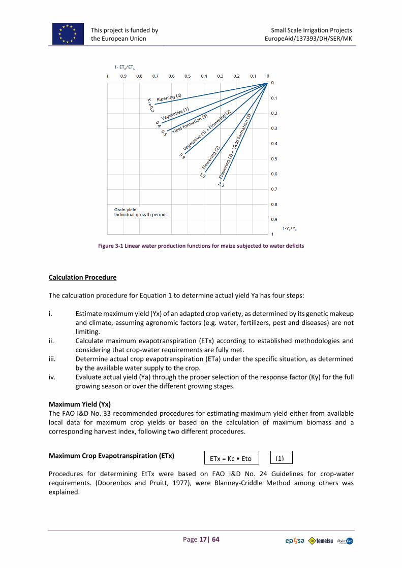
The analysis of deficit irrigation studies also allowed, for a majority of crops, the development of crop response functions when water deficits occur at different crop stages. As illustrated for maize in Figure 2.1, yield response will differ largely depending on the stage the water stress occurs. Typically flowering and yield formation stages are sensitive to stress, while stress occurring during the ripening phases has a limited impact, as in the vegetative phase, provided the crop is able to recover from stress in subsequent stages. In Figure 2.1, the linear water production functions for maize subjected to water deficits occurring during the vegetative, flowering, yield formation and ripening periods are shown. The steeper the slope (i.e. the higher the Ky value), the greater the reduction of yield for a given reduction in ET because of water deficits in the specific period.
This project is funded by the European Union
Small Scale Irrigation Projects EuropeAid/137393/DH/SER/MK
Page 17| 64
Figure 3-1 Linear water production functions for maize subjected to water deficits
Calculation Procedure The calculation procedure for Equation 1 to determine actual yield Ya has four steps: i. Estimate maximum yield (Yx) of an adapted crop variety, as determined by its genetic makeup
and climate, assuming agronomic factors (e.g. water, fertilizers, pest and diseases) are not limiting.
ii. Calculate maximum evapotranspiration (ETx) according to established methodologies and considering that crop-water requirements are fully met.
iii. Determine actual crop evapotranspiration (ETa) under the specific situation, as determined by the available water supply to the crop.
iv. Evaluate actual yield (Ya) through the proper selection of the response factor (Ky) for the full growing season or over the different growing stages.
Maximum Yield (Yx) The FAO I&D No. 33 recommended procedures for estimating maximum yield either from available local data for maximum crop yields or based on the calculation of maximum biomass and a corresponding harvest index, following two different procedures.
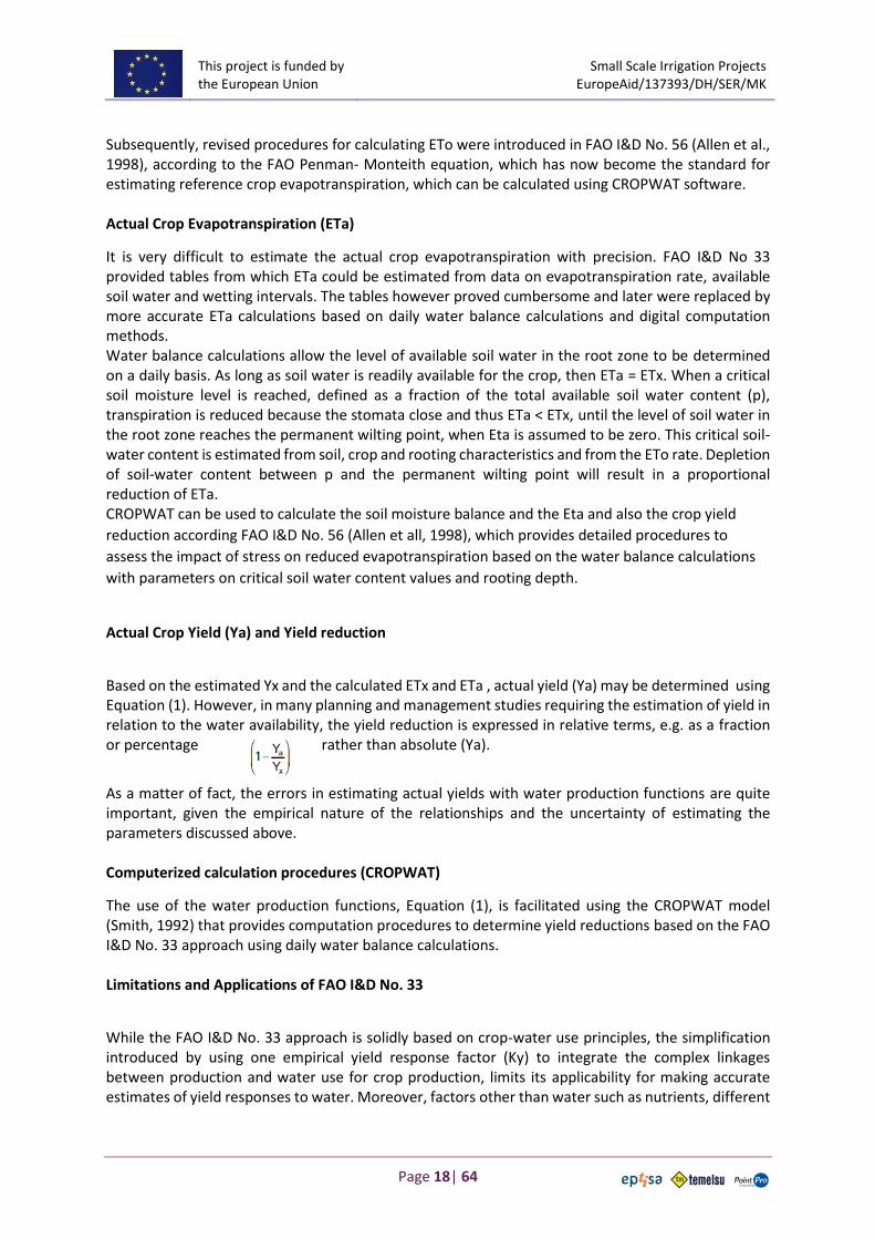
Maximum Crop Evapotranspiration (ETx) Procedures for determining EtTx were based on FAO I&D No. 24 Guidelines for crop-water requirements. (Doorenbos and Pruitt, 1977), were Blanney-Criddle Method among others was explained.
ETx = Kc • Eto (1)
This project is funded by the European Union
Small Scale Irrigation Projects EuropeAid/137393/DH/SER/MK
Page 18| 64
Subsequently, revised procedures for calculating ETo were introduced in FAO I&D No. 56 (Allen et al., 1998), according to the FAO Penman- Monteith equation, which has now become the standard for estimating reference crop evapotranspiration, which can be calculated using CROPWAT software. Actual Crop Evapotranspiration (ETa)
It is very difficult to estimate the actual crop evapotranspiration with precision. FAO I&D No 33 provided tables from which ETa could be estimated from data on evapotranspiration rate, available soil water and wetting intervals. The tables however proved cumbersome and later were replaced by more accurate ETa calculations based on daily water balance calculations and digital computation methods. Water balance calculations allow the level of available soil water in the root zone to be determined on a daily basis. As long as soil water is readily available for the crop, then ETa = ETx. When a critical soil moisture level is reached, defined as a fraction of the total available soil water content (p), transpiration is reduced because the stomata close and thus ETa < ETx, until the level of soil water in the root zone reaches the permanent wilting point, when Eta is assumed to be zero. This critical soil-water content is estimated from soil, crop and rooting characteristics and from the ETo rate. Depletion of soil-water content between p and the permanent wilting point will result in a proportional reduction of ETa. CROPWAT can be used to calculate the soil moisture balance and the Eta and also the crop yield
reduction according FAO I&D No. 56 (Allen et all, 1998), which provides detailed procedures to
assess the impact of stress on reduced evapotranspiration based on the water balance calculations
with parameters on critical soil water content values and rooting depth.
Actual Crop Yield (Ya) and Yield reduction
Based on the estimated Yx and the calculated ETx and ETa , actual yield (Ya) may be determined using Equation (1). However, in many planning and management studies requiring the estimation of yield in relation to the water availability, the yield reduction is expressed in relative terms, e.g. as a fraction or percentage rather than absolute (Ya).
As a matter of fact, the errors in estimating actual yields with water production functions are quite important, given the empirical nature of the relationships and the uncertainty of estimating the parameters discussed above. Computerized calculation procedures (CROPWAT)
The use of the water production functions, Equation (1), is facilitated using the CROPWAT model (Smith, 1992) that provides computation procedures to determine yield reductions based on the FAO I&D No. 33 approach using daily water balance calculations. Limitations and Applications of FAO I&D No. 33
While the FAO I&D No. 33 approach is solidly based on crop-water use principles, the simplification introduced by using one empirical yield response factor (Ky) to integrate the complex linkages between production and water use for crop production, limits its applicability for making accurate estimates of yield responses to water. Moreover, factors other than water such as nutrients, different

This project is funded by the European Union
Small Scale Irrigation Projects EuropeAid/137393/DH/SER/MK
Page 19| 64
cultivars, etc. also affect the response to water. Adjustments for site-specific conditions would be needed if greater accuracy is sought. As an example of the differences in Ky values from different studies, it is instructive to compare the results under a cooperative research programme carried out by the International Atomic Energy Agency (IAEA) against the original Ky values of the FAO I&D No. 33. Table 2.2 summarizes the comparison of Ky values. No specific trend can be extracted from the deviations in the Ky values under different conditions. It can be concluded that application of the water production function approach has proved useful for general planning, design and operation of irrigation projects and for the rapid assessment of yield reductions under limited water supply. For improved strategies and practices related to on-farm water management aiming to increasing efficiency and productivity of water use, Equation 1 is of limited use and more accurate predictions are required for yield response under actual field conditions. AquaCrop, which is described in the available software for irrigation, provides a valid alternative for herbaceous crops, as the incorporation of advanced knowledge of crop-water relationships allows a more accurate modelling of actual crop growth and yield formation processes under various soil water availability, climate and soil fertility conditions.
3.5 THE PROGRAM STRUCTURE
The main “route“ through the program follows the menu options along the top of the screen, and you can also access the data entry windows using the icons in the Input Modules at the left
The input modules 1. Climate/ETo: 2. Rain: 3. Crop 4. Soil 5. Crop pattern
The calculation modules 6. Crop Water Requirements (CWR) 7. Schedules 8. Scheme

This project is funded by the European Union
Small Scale Irrigation Projects EuropeAid/137393/DH/SER/MK
Page 20| 64
3.5.1 INPUT MODULES
First Step – Insert all required inputs
As you work with the program, you will often find that there are several ways of getting to the same menu option. For example, you can input the climate data in the Climate/Eto module or in the menu option at the top, File/New/Climate-ETo/
Climate or Eto
1. Reference Crop Evapotranspiration (ETo) values calculated from- either measured values entered directly from the keyboard using File/New/ Climate-ETo/, where you can enter monthly, decade or daily measured Eto, or Estimates of ETo calculated using the Penman-Monteith equation. ETo is automatically calculated when you enter monthly/decade or daily climatic data (temperatures, humidity, windspeed, sunshine). The data can be introduced from the keyboard or from a data file using Climate-Eto module/Open.

This project is funded by the European Union
Small Scale Irrigation Projects EuropeAid/137393/DH/SER/MK
Page 21| 64
Obtaining data from CLIMWAT Once you have installed the CLIMWAT database in your computer, you can obtain the climatic data in two ways:
1) Introduce the coordinates of the location you are interested to get data from and the number of stations to be selected, and the database will return the neighbouring stations to that location
2) Choose the country and select the climatological station in / in and around that country.
CLIMWAT will show a map with the available stations, which in the case of Macedonia are:
The coordinates and altitude of the SKOPJE meteorological station in CLIMWAT correspond to a location in Serbia, as it is shown in the CLIMWAT map. The data is then doubtful and should be checked with actual data from Skopje Meteorological station. Two files are created for each selected station: .CLI file: The first file contains long-term monthly rainfall data [mm/month]. Additionally, effective
rainfall is also included calculated and included in the same file. .PEN file: The second file consists of long-term monthly averages for the seven climatic parameters, mentioned above. This file also contains the coordinates and altitude of the location. There are 3 methods to work with CROPWAT if not all meteorological data is data available:
1) Obtain data from CLIMWAT

This project is funded by the European Union
Small Scale Irrigation Projects EuropeAid/137393/DH/SER/MK
Page 22| 64
2) CROPWAT based in temperature data can estimate relative humidity, sunshine duration and windspeed;
3) Meteorological data can be estimated using the available data form surrounding
stations. More information in Allen et al, 1998.
By any of the above methods you will obtain finally the completed tables for Climate/Eto values:
At the bottom of the page, the name of the files you are using will be shown.
In the Options menu bar, 5 different methods can be used for calculation of the effective rainfall. The defect option is the USDA Soil Conservation Service Formula.
If some relative humidity, sunshine duration and windspeed data is missing, if the temperature data is available, CROPWAT can estimate the missing values using the ESTIMATE (F6) button.

This project is funded by the European Union
Small Scale Irrigation Projects EuropeAid/137393/DH/SER/MK
Page 23| 64
Estimation relative humidity, sunshine duration and windspeed data based in temperature data
using CROPWAT
In the Options menu, you can choose “Eto Penman calculated from temperature data (other data
estimated). The changes in this setting will only affect NEW data, so you first have to choose this
option. In this screen you can When you open the
The values obtained based just in Temperature using CROPWAT are:
In the particular case of SKOPJE meteorological Station, the values calculated based only in
temperature data lead to a higher ETo than the ones using all the available data.
In Annex 2 there are included the data obtained during preparation of Feasibility Studies for the
following meteorological stations: Strumica, Kichevo and Kriva Palanca. (for average, day and humid
years).
Eto CLIMWAT Difference
mm/day %
0,54 -17%
0,82 -26%
1,58 -10%
2,76 -13%
3,41 -16%
4,31 -17%
5,19 -9%
4,6 -15%
3,28 -14%
1,7 -21%
0,89 -18%
0,61 -18%
2,47 -15%

This project is funded by the European Union
Small Scale Irrigation Projects EuropeAid/137393/DH/SER/MK
Page 24| 64
The effective rainfall (8) is the total rainfall (1) minus
runoff (4) minus evaporation (5) and minus deep
percolation (7). We used previously the FAO formula:
Pe = 0.8 (P – 25) if Pmonthly > 75 mm/month
Pe = 0.6 (P - 10) if Pmonthly < 75 mm/month
with P = rainfall or precipitation (mm/month)
Pe = effective rainfall or effective precipitation (mm/month) (NOTE: Pe is always equal to or larger than zero; never negative).
In the previous training, we have obtain similar results using Blaney Criddle Method and performing the calculations without using a computer:
After completion of the climatic data and the rain data, it is possible to obtain tables with the
calculated values of ETo and Effective Rainfall:

This project is funded by the European Union
Small Scale Irrigation Projects EuropeAid/137393/DH/SER/MK
Page 25| 64
Acording to CROPWAT, the Eto (grass
evapotranspiration) is 906,71 mm/year in
average, or 906,71 / 360 = 2,52 mm/day.
The table of average daily water need of
standard grass during irrigation season
values (Brouwer & Heibloem, 1986)
confirms that with an average temperature
of (6,0+18,4)/2= 12,2 °C < 15 °C and a 69%
humidity, Skopje has a Humid Climate with
low mean daily temperature, and the
values of Eto according to the table are 1-2
mm/day
It is also possible to obtain charts with the graphic display of all data in bars or lines:
According to the chart, in Skopje grass should be irrigated from March to September
CROP DATA
The next step is the calculation of the Crop Water Needs:
We can go to the crop input module, and open the file provided by
CROPWAT for Tomatoes, for example.
As in the previous training, it is important to determine based in the local data, the duration of the
growing period, the planting date and the rooting depth. In the provided file included in CROPWAT,
we have to correct the provided values to, for example, a growing period of 150 days from sowing,
and a planting date of 15/04

This project is funded by the European Union
Small Scale Irrigation Projects EuropeAid/137393/DH/SER/MK
Page 26| 64
CROPWAT calculates the critical depletion factor and the yield response coefficients following the
described calculation procedure.( FAO I&D No. 33) (Doorenbos and Kassam,1979).
Notice that the crop data will be shown in the bottom line. IF you change the FAO crop values, it is
better to save the crop as a particular crop you have corrected. (File/Save)
SOIL DATA
The soil available water content
(or available soil moisture), AWC
= FC – WP), the maximum
infiltration rate, the maximum
rooting deph (check with the
value you have just entered for
the crops) and the initial moisture
depletion should be filled, or the
data uploaded from an existing
file using the Soil Input
module/Open. Notice that the
provide data includes the Critical
Depletion fraction, the Crop Yield
Response factor and the Cropheight, which are used for the determination of Yields Reductions. IF
you change the FAO soil values, it is better to save the crop as yours particular soil. (File/Save)

This project is funded by the European Union
Small Scale Irrigation Projects EuropeAid/137393/DH/SER/MK
Page 27| 64
3.5.2 CALCULATION MODULES
CROP WATER REQUIREMENT (CWR) (ET CROP) and IRRIGATION REQUIREMENT
From the CWR module you can obtain the calculated ETC for
Tomatoes, using the Penman – Monteich method. If you
substract the effective rain you get the Irrigation Requirement.
The total evapotranspiration for Tomato calculated is 595 mm for the entire growing season. The
indicative values provided by Brouwer & Heibloem, 1986 are for Tomato:
Crop Crop water need
(mm/total growing period) Sensitivity to drought
Tomato 400-800 medium-high
Then, our calculation for Tomatoes grown in Skopje are in the expected range of values. CROPWAT
also provides a chart for the ETc and the Irrigation requirement.

This project is funded by the European Union
Small Scale Irrigation Projects EuropeAid/137393/DH/SER/MK
Page 28| 64
IRRIGATION SCHEDULE
The Schedule calculation module lets you define how irrigations are calculated and to manage groups
of data files (climate,rain,crop,soil) which are called “irrigation Sessions”. At this stage, all you need
to do is to define the method for scheduling using Schedule, Criteria.
The Table format can appear in two ways, which are selected in the Options box at the top of the
form. The options are either
• Irrigation Schedule: This table shows the status of the soil moisture every time new water
enters the soil, either by rainfall or a calculated irrigation application. Calculated irrigation
events are shown in the right hand side of the table (Net Irrigation/Irrigation Interval); the
other lines in the table are where rainfall events occur as defined in the Options menu
(e.g. a rain event every 5 days).
• Daily Soil Moisture Balance: This shows the status of the soil every day throughout the
cropping pattern. It is useful in seeing how the soil moisture changes in the growing season,
but the table is much longer and contains possibly too much information for most users.
Graphs can be used to show these changes more clearly. User defined irrigation events and
other adjustments to the daily soil moisture balance can be made when the Scheduling
Criteria are set to “user defined”. This provides a flexible system to simulate actual changes
in water use during the growing season. The recorded rain can be introduced after every
rainfall event, and the Soil Moisture Balance will be automatically updated
You can modify the scheduling criteria using the Options menu.

This project is funded by the European Union
Small Scale Irrigation Projects EuropeAid/137393/DH/SER/MK
Page 29| 64
If you use the FAO defaults, you will get an optimal irrigation schedule
The irrigation timing is variable, you irrigate when the ready readily available soil moisture (RAM) is
depleted. (RAM : Readily Available Moisture in the soil for the crop at this date (mm). It is calculated
as RAM = TAM * P where P is the depletion fraction for this crop at the current date as defined in
the crop data screen).
The amount of irrigation is also variable: you irrigate to refill to the Field Capacity (FC).
The irrigation schedule table can be printed at the Print
menu.

This project is funded by the European Union
Small Scale Irrigation Projects EuropeAid/137393/DH/SER/MK
Page 30| 64
• The coefficient between Total net and gross irrigation if the application efficiency: 0.7
• The schedule has no deficit and no irrigation losses. The schedule efficiency is 100%
• The irrigation schedule shows only the days when irrigation is provided. Therefore, there
are no rain events. But they are taking into consideration. If the soil moisture balance
option is selected, then the rain events are shown:
6 6 5 10

This project is funded by the European Union
Small Scale Irrigation Projects EuropeAid/137393/DH/SER/MK
Page 31| 64
The irrigation flow [l/s ha] considers 1 ha of tomato
𝐼𝑟𝑟. 𝐹𝑙𝑜𝑤 [𝑙
𝑠 ℎ𝑎] =
9,5 𝑚𝑚
𝑑𝑎𝑦∗ 1 ℎ𝑎 ∗
10000 𝑚2
ℎ𝑎 *
1 𝑚
1000 𝑚𝑚 *
1000 𝑙
1 𝑚3*
1 𝑑𝑎𝑦
86400 𝑠 = 1,1 [l/s ha]
ANOTHER SCHEDULING OPTIONS
It is possible to use another scheduling options than the FAO defaults. In the Options menu, we can
choose the following irrigation timings, application options and change the application efficiency:
Irrigation timing options Irrigation application options
Change Irrigation Application Efficiency

This project is funded by the European Union
Small Scale Irrigation Projects EuropeAid/137393/DH/SER/MK
Page 32| 64
Cropwat can be used to evaluate also rainfed crops.
SOME EXAMPLES:
1. Check user proposed irrigation scheduling
With the Estimation Method in a Humid climate with low temperature and sandy soils, the
recommended schedule for tomatoes is 30 mm every 6 days:
We can check with CROPWAT what is the result of the recommended schedule for tomatoes growing in Skopje:
Irrigation losses
Water shortage -> Yield Reduction

This project is funded by the European Union
Small Scale Irrigation Projects EuropeAid/137393/DH/SER/MK
Page 33| 64
In this case, the tomatoes needed 591 mm during the whole growing season, and the net irrigation depth provided was 720 mm, 278 mm were lost by deep percolation at the beginning of the growing season, when the root system is shallow and could not use all the provided water. The schedule has

This project is funded by the European Union
Small Scale Irrigation Projects EuropeAid/137393/DH/SER/MK
Page 34| 64
only a 61% of efficiency. Then Yield reduction is 0,2%. Then, the schedule is adequate for the agricultural production, but it is not very efficient in the water use. The Estimation Method suggested to adjust the schedule in order to save water,
• during the early stages of the crop development, with smaller irrigation applications
• during the late stage it may be feasible to irrigate less frequently We can change the application to 10 mm in the initial stage, 15 in development and 30 in mid and late season, and change in late season to an 8 days interval.

This project is funded by the European Union
Small Scale Irrigation Projects EuropeAid/137393/DH/SER/MK
Page 35| 64
In this case, the tomatoes as always needed 591 mm during the whole growing season, and the net irrigation depth provided was 500 mm, and 278 mm were lost by deep percolation. The schedule has only a 88% of efficiency. The Yield Reduction increased from 0,2 to 0,4%.
You can simulate as many different irrigation depths and timing.
2. Check feasibility of rainfed cropping.
If we choose the rainfed option, to check is tomatoes can be grown in Skopje without irrigation:
Only 245 mm were provided of the 592 mm needed by the tomatoes. The reduction of yield is 62%., considering an average meteorological year and that the monthly precipitation is divided in 5 events of the equal value.
Each of these variants can be stored as a “Session” in the File Menu. The File Locations in the hard drive can be modified at the Settings Menu:

This project is funded by the European Union
Small Scale Irrigation Projects EuropeAid/137393/DH/SER/MK
Page 36| 64
3. Perform calculation of Irrigation Scheduling and/or Daily Soil Moisture Balance taking in account:
• non-standard irrigation schedules irrigation applications.
• actual rain
To model what actually takes place in a growing season it is necessary to enter specific irrigation applications on given dates. A wide range of options are available in the Scheduling Criteria. The impact of non-standard irrigation schedules can be examined by setting the irrigation timing option to “Irrigate at user defined intervals” and the irrigation application to “User defined application depth” -i.e. scheduling with variable dates and amounts of irrigation. You can also use the option of modifying the net irrigation column in the Irrigation Scheduling and/or Daily Soil Moisture Balance. In these case the timing and application depth considered for the generation of the table get in red colour and between brackets there is a notice saying (adjusted by user).
This can be useful if you want to calculate a real daily soil moisture balance taking into consideration the rain measurements obtained from a local meteorological station or your own pluviometer. In this case, the rainfall option should be “Rainfall not considered in irrigation calculation (effective rain = 0)”
Irrigation timing options Irrigation application options
Change Irrigation Application Efficiency

This project is funded by the European Union
Small Scale Irrigation Projects EuropeAid/137393/DH/SER/MK
Page 37| 64
FARM OR SCHEME IRRIGATION NEEDS
CROPPING PATTERN
In a farm, or a given bigger area, there are more than one crop being cropped at the same time. For this scheme, the irrigation flow requirements can be calculated based on the scheme's cropping pattern. The cropping pattern, or cropping schedule of an irrigation area provides information, for a period of at least one season, on three important elements: - which crops are grown - when are they cultivated - how many hectares of each crop are grown. CROPWAT can calculate crop water requirements or irrigation schedules with up to 30 crops. Each crop in the pattern is defined by the crop coefficient file name, the date of planting and the area planted (0-100% of the total area). Each crop may be planted in a set of blocks staggered in time. SAMPLE PROBLEM: Determine the farm (or scheme) irrigation needs based on the following assumed data. Assumptions:
Crop 1 Crop 2 Crop 3
Name: Alfalfa perennial Potato Tobacco
% Area: 30 10 60
Planting period 1 April – 30 March 1 April 15 arch 5 April
Growing period 365 days 130 days 110 days
In the CROPWAT 4.2 version, the software was able to calculate crop water requirements or irrigation schedules with up to 30 crops and each crop could be calculated as planted in a set of blocks staggered in time, using the Option menu in the Cropping pattern module.

This project is funded by the European Union
Small Scale Irrigation Projects EuropeAid/137393/DH/SER/MK
Page 38| 64
In the 8.0 version of CROPWAT this is not any more possible. Therefore, in order to take into consideration different staggered blocks of a crop, you should consider them as different crops with different planting dates. For ejample, in the case of Tobacco which is staggered between 15/03 and 15.4, we can introduce 3 tobaccos with 1/3 of the total tobacco area, plated every 10 days.
The 8.0 version does not plot the cropping pattern either. For each of the considered crops, you will get an irrigation schedule/daily soil moisture balance chart and table. Each crop will have its own scheduling criteria.
Crop 1 Crop 2 Crop 3
Alfalfa perennial Potato Tobacco
FARM OR SCHEME IRRIGATION NEEDS
In the Scheme module, you caobtain the irrigation needs table for all the farm or scheme.
RAM
TAM
Depletion
Days after planting
360350340330320310300290280270260250240230220210200190180170160150140130120110100908070605040302010
Soil
wate
r re
tentio
n in
mm
160
140
120
100
80
60
40
20
0
-20
Field CapacityField CapacityField Capacity

This project is funded by the European Union
Small Scale Irrigation Projects EuropeAid/137393/DH/SER/MK
Page 39| 64
4 DESIGN AND EVALUATION OF SURFACE IRRIGATION SYSTEMS: SIRMOD MODEL
(WALKER, 2003)
Surface irrigation system should replenish the root zone reservoir efficiently and uniformly so crop
stress is avoided. The design procedures outlined in the following sections are based on a target
application depth, zreq
, which equals the soil moisture extracted by the crop.
Design is a trial and error procedure. A selection of lengths, slopes, field inflow rates and cutoff times
can be made that will maximize application efficiency for a particular configuration. Iterating through
various configurations provide the designer with information necessary to final a global optimum.
Considerations such as erosion and water supply limitations will act as constraints on the design
procedures. Many fields will require a subdivision to utilize the total flow available within a period of
availability. Maximum application efficiencies, the implicit goal of design, will occur when the least-
watered areas of the field receive a depth equivalent to zreq
. Minimizing differences in intake
opportunity time will minimize deep percolation. Surface runoff will be controlled or reused.
4.1 SURFACE IRRIGATION SYSTEM DESIGN
There are five primary surface irrigation configurations:
Free-draining systems: tailwater runoff is allowed. However, this reduces application efficiency,
may erode soil or cause similar problems. It is therefore not a desirable surface irrigation
configuration. However, where water is inexpensive the costs of preventing runoff or capturing
and reusing it may not be economically justifiable to the irrigator. In addition, ponded water at
the end of the field represents a serious hazard to production if the ponding occurs over sufficient
time to damage the crop
Blocked-end systems; Blocking the end of basin, border, or furrow systems provides the designer
and operator with the capability of achieving potential application efficiencies comparable with
most sprinkle and drip irrigation systems. Of course the sprinkle and drip systems are more easily
managed for high efficiencies. They also represent the highest risk to the grower. Even a small
mistake in the cutoff time can result in substantial crop damage. Consequently, all blocked-end
surface irrigation systems should be designed with emergency facilities to drain excess water from
the field.

This project is funded by the European Union
Small Scale Irrigation Projects EuropeAid/137393/DH/SER/MK
Page 40| 64
Free-draining systems with cutback: Cutback is a concept of having a high initial flow (to speed the
advance phase) and a reduced flow thereafter (to minimize tailwater). A common practice is
reducing the inlet discharge by roughly one-half when the flow reaches the end of the field. As a
practical matter however, cutback systems have never been very successful. They are rigid
designs in the sense that they can only be applied to one field condition. Thus, for the condition
they are designed for, they are efficient but as the field conditions change between irrigations or
from year to year, they can be very inefficient and even ineffective.
Free-draining systems with tailwater recovery and
reuse: The application efficiency of free-draining
surface irrigation systems can be greatly improved
when tailwater can be captured and reused. If the
capture and reuse is to be applied to the field
currently being irrigated, the design is more complex
because you need to use two sources of water
simultaneously. The major complexity of these reuse
systems is the strategy for re-circulating the
tailwater:
• pump the tailwater into the primary supply:
the reservoir would collect the runoff of one
set of furrows or basins, pump to the primary supply and combine it with the supply to a
second set
• reuse will occur on another field: , the reservoir would collect the runoff and then supply
the water to the headland facilities of the other field. This requires a larger tailwater
reservoir but perhaps eliminates the need for the pump-back system
Surge flow systems: Surge irrigation is the intermittent
application of water to a furrow and under the surge flow regime,
irrigation is accomplished through a series of short duration
pulses of water onto the field. With continuous furrow irrigation,
as soon as water is applied to the furrow, it begins to infiltrate
downward and laterally throughout the root zone of the crop.
Initially, the advance rate is fast, but as the water advances down
the furrow, the advance rate slows. Water infiltration can be
much greater at the top of the field than the bottom because of
the longer opportunity time. Instead of providing a continuous
flow onto the field, a surge flow regime would replace a 6-hour
continuous flow set with something like six 40-minute surges.
The intermittent application
• reduces infiltration rates (over at least a portion of the field: the wetted parts)
• increases advance rates (over the wetted parts)
• intake opportunity times over the field are more uniform

This project is funded by the European Union
Small Scale Irrigation Projects EuropeAid/137393/DH/SER/MK
Page 41| 64
• reduces the time necessary for the infiltration rates to approach the final or basic rate.
• less water is required to complete the advance phase by surge flow than with continuous
flow
• runoff is reduced
To achieve this effect on infiltration rates, the flow must completely drain from the field between
surges. If the period between surges is too short, the individual surges overlap, and the infiltration
effects are generally not created.
Surge irrigation may not be an improvement on:
• soils that initially have low intake rates and soils that crack when dry.
• fields with relatively large slopes.
Surging is often the only way to complete the advance phase in high intake conditions like those
following planting or cultivation.
AUTOMATION: Surge flow lends itself very well to automation which greatly enhances the use of
cutback irrigation. The automation reduces the labor requirement. Automated butterfly valves
implement surge flow by sequentially diverting the flow from one bank of furrows to another on either
side of the valve. The automated butterfly valves have two main components: a butterfly valve and a
controller. The valve body is an aluminum tee with a diverter plate that directs water to each side of
the valve. The controller uses a small electric motor to switch the diverter plate. Controllers can be
adjusted to accomplish a wide variety of surge flow regimes and have both an advance stage and a
cutback stage. During the advance stage, water is applied in surges that do not overlap and can be
sequentially lengthened. Specifically, it is possible to expand each surge cycle so surges that wet the
downstream ends of the field are longer than those at the beginning of irrigation. During the cutback
stage, the cycles are shortened so the individual surges do overlap.
4.2 PROGRAM STRUCTURE
DATA INPUT: it involves two activities:
(1) defining the characteristics of the surface irrigation system under study; and

This project is funded by the European Union
Small Scale Irrigation Projects EuropeAid/137393/DH/SER/MK
Page 42| 64
(2) defining the model operational control parameters.
Entering Field Characteristics (Input/Field Topography –Geometry)
The geometry and topography of the surface irrigated field is described by the following
parameters:
Field length; Field width; Field cross-slope; Unit spacing for borders and basins, or furrow spacing; Field System: (free draining or blocked end) Manning roughness, n, for the first irrigations; Manning roughness, n, for later irrigations; 3 slope values in the direction of flow; and 2 distances associated with the 3 slopes. Flow cross section: the flow cross-section is defined and computed with four parameters,
top width, middle width, base, and maximum depth. As these are entered eight parameters labeled Rho1, Rho2, Sigma1, Sigma2, Gamma1, Gamma2, Cch, and Cmh are automatically computed.
Infiltration Functions This is the most critical component of the SIRMOD III software. Four individual infiltration functions
are required:
(1) a function for first conditions under continuous flow; (2) a function for later irrigations under continuous flow; (3) a function for first irrigations under surge flow; and (4) a function for later irrigations under surge flow

This project is funded by the European Union
Small Scale Irrigation Projects EuropeAid/137393/DH/SER/MK
Page 43| 64
Each infiltration function requires four parameters, k, a, fo, and C. The parameter Qinfilt
is the
flow where the various infiltration parameters are referenced. If the user does not know this
value, the discharge used in the simulation should be input in this edit box.
Immediately below the four infiltration coefficients for the various surface irrigation regimes are
four buttons labeled “Tables”. These buttons access four default infiltration data
Below the four “Tables” buttons are four edit boxes for displaying the required infiltration depth, Zreq, and the associated intake opportunity time, τreq. The user can input data directly into either the Zreq or the τreq boxes and the program will compute the other parameter automatically. The remaining button labeled “Two-Point ” and the three edit boxes labeled T
L, T
.5L, and .5L will be
discussed at the 4.1 EVALUATION section.

This project is funded by the European Union
Small Scale Irrigation Projects EuropeAid/137393/DH/SER/MK
Page 44| 64
ENTERING MODEL CONTROL PARAMETERS
SIRMOD includes three modelling choices: (1) kinematic-wave model; (2) zero-inertia model; and (3) hydrodynamic model. The default is the hydrodynamic model. The user may choose a particular model for simulation by clicking their associated check boxes. Simulation Shutoff Control
The termination of field inflow for the purposes of simulation is either by specifying a total inflow interval or by specifying a fixed depth of application. The interval will over-ride the depth control, so when using depth control the user should make the interval a large number Inflow Regime
SIRMOD will simulate both continuous and surge flow irrigation. There are three continuous and four surge flow regimes. The user may select one regime at a time for simulation by clicking on the respective check box. Both continuous and surged systems can operate with a cutback regime, although the only practical application of the concept is via surge flow. Under a surge flow regime, there are two cycle options.
• Fixed cycle time surge flow system: by multiplying the first surge cycle by a user-specified fraction (See the “Surge Adj. Ratio” edit box). For example, if the first surge is 30 minutes and it is desirable to expand the surges by 10% each cycle, then the “Surge Adj. Ratio” can be set to 1.1.
• Variable cycle time option: by adding a fixed amount of time to each surge via the “Surge Adj Time” parameter. For instance if one begins with a 60 minute cycle and wish to expand it 10 minutes each surge, then the “Surge Adj Time” parameter is set to 10.
In both cases of variable cycle surge flow, the cycle times can be compressed by specifying a value less than 1.0 or a negative value “Surge Adj. Ratio”.

This project is funded by the European Union
Small Scale Irrigation Projects EuropeAid/137393/DH/SER/MK
Page 45| 64
Flow control parameters There are nine flow control parameters:
(1) Simulated Unit Inflow;
(2) Time of Cutoff;
(3) Dtm
(4) Number of Surges;
(5) Surge On Time
(6) Cutback Ratio;
(7) CB Length fraction
(8) Surge Adj. Ratio; and
(9) Surge Adj. Time.
Special numerical coefficients These coefficients are computed automatically by the software. For the typical simulation, the user need not alter them. They can be changed however should the user wish. Details of these parameters are given in (Walker,2003). SIMULATION
Once the input and control data have been entered, the simulation is executed by clicking on the button. The simulation screen will appear and the run-time plot of the advance and recession profiles will be shown as illustrated
There are three important regions in the simulation screen:
Upper half of the screen: plots the surface and subsurface movements of water as the advance
and recession trajectories are computed. The target or required depth of application is plotted

This project is funded by the European Union
Small Scale Irrigation Projects EuropeAid/137393/DH/SER/MK
Page 46| 64
as Zreq so that when an infiltrated depth exceeds this value the user can see the loss of
irrigation water to deep percolation
Lower right side of the screen: a summary of the simulated
irrigation event:
The application efficiency: represents the fraction of water applied to the field that could be considered beneficially used
V
rz is the volume of water that is actually stored in the root zone
VL is the volume of of water needed for leaching.
Vin is the volume of water applied to the field.
Vdp
is the volume of water that percolates below the root zone.
Vtw
is the volume of water that flows from the field as tailwater.
(NOTE: all volumes are referred per unit width or per furrow spacing)
The requirement efficiency is a measure of how well the root zone was refilled (also called storage).
V
di is the volume that is represented as the under-irrigation
The application efficiency: is a subset of irrigation efficiency, which evaluates only how well the irrigation water was stored in the root zone:
The application uniformity: is the average infiltrated depth in the low quarter of the field divided by the average infiltrated depth over the whole field. Also an 'absolute distribution uniformity', DU
a is suggested which is the minimum depth divided by the average depth. Thus:
Zlq
is the average depth of infiltrated water in the least-irrigated 25% of the
field. Z
min is the minimum depth of infiltration applied to the field, often but not
always located at the downstream end of the field.
The bottom four edit windows give a mass balance of the simulation, including an error term describing the computed differences between inflow, infiltration, and runoff (if the field is not diked). As a rule an error less than 5% is acceptable – most simulations will have errors of about 1%.

This project is funded by the European Union
Small Scale Irrigation Projects EuropeAid/137393/DH/SER/MK
Page 47| 64
Lower left side of the screen, a runoff hydrograph will be plotted for the cases where the downstream end of the field in not diked. NOTE: that neither the advance-recession nor the runoff hydrograph are intended to be quantitative, as no units are included in the plot. These details are presented in the plotted and printed output from the model.
4.3 THE DESIGN PROCESS
The surface irrigation design process is a procedure matching the most desirable frequency and depth of irrigation with the capacity and availability of the water supply. This process can be divided into a preliminary design stage and a detailed design stage.
The Preliminary Design :
1) Determination of water supply availability: continuous, rotational (flow rate and duration may
be relatively fixed) or on demand.
2) Determination of Crop water demand (climate, soil and cropping patterns)
3) Determination of a tentative schedule.
4) Determination of the type of surface irrigation method (Furrow, basin) according to slopes, stream size, soil, row crops, etc.
Detailed Design
1) Determination the slope of the field, the furrow, border or basin inflow discharge (stream size) and duration, surface drainage facilities either to collect tailwater for reuse or for disposal, land levelling. Field length becomes an important design variable (mechanized, animal power, hand labour?) Long rectangular fields are preferable to short square ones in most cases.
2) Reconciliation of flows and times with the total flow and its duration. On small fields, the total supply may provide a satisfactory coverage when used to irrigate the whole field simultaneously. However, the general situation is that fields must be broken into 'sets' and irrigated part by part, i.e. basin by basin, border-by-border, etc.
3) Operation means: pipes, ditches, control elements, automation, labour force available, etc.must be sized for the field. If tailwater is permitted, means for removing these flows must be provided.
4) Use SIRMOD to compute the optimal values of inflow discharge and time of cutoff for the
field configuration selected by the user. The philosophy of design suggested is to evaluate flow rates and cutoff times for the first irrigation following planting or cultivation when roughness and intake are maximum, as well as for the third or fourth irrigation when these conditions have been changed by previous irrigations. This will yield a design that will have the flexibility to respond to the varying conditions the irrigator will experience during the season.
4.4 THE EVALUATION PROCESS
The data necessary to evaluate an irrigation event would include an inflow-outflow hydrograph, advance and recession trajectories, flow geometry, field slope, length, and roughness and infiltration characteristics. These conditions require a maximum of 16 individual parameters whose variations

This project is funded by the European Union
Small Scale Irrigation Projects EuropeAid/137393/DH/SER/MK
Page 48| 64
can vary by as much as an order of magnitude. Thus, developing a comprehensive understanding of their interrelationships would require an enormously expensive and time-consuming field investigation program. A process applicable is described in Annex I. The alternative to research through field evaluation is through theoretical study. Mathematical relationships are formulated and then verified by selective comparison with field observations. Field data collection is still required, but less often and more carefully determined.
Field Evaluation Procedure An evaluation of a surface irrigation system usually considers the field water balance discussed in Chapter 2 (see p. 2-2, Eq. 2.2). In most cases a short period to time extending no 1) The general layout of the field: head pipes or
ditches, tailwater drainage, cropping patterns
2. The field geometry and topography: length, width,
slope and in the case of furrow irrigation, the
furrow shape
3. The amount of water that should be applied measuring the soil moisture using a method such as gravimetric sampling, tensiometer, electrical resistance blocks, neutron probes, etc. The number and spatial distribution of measurements will impact the accuracy of the measurement. These measurements should be made immediately before irrigation and within 3 days afterwards. 4. The inflow hydrograph (per furrow or per border or basin) needs to be measured carefully. If possible, the inflow should be controlled at one value during the entire evaluation.
5. The advance and recession of the water over the field surface, measured as the elapse time needed for the inflow to advance to a point on the field, or the elapse time until water has drained from the point following the cutoff of inflow, is required and should be among the most carefully made measurements in the field
In surface irrigation evaluations, the values of Q
inf, the discharge intering the furrow/basin and
the time that takes the water to arrive during the advance phase to two points x = 0.5L and x =

This project is funded by the European Union
Small Scale Irrigation Projects EuropeAid/137393/DH/SER/MK
Page 49| 64
L where L is the length of the field, m. Thus, the values of time that are measured are t.5L
and
tL.
6. The runoff hydrograph (if the field is not diked), measured in the same manner as inflow;
Software evaluation process
The evaluation of infiltration coefficients from advance data is initiated by pressing the button on the
Infiltration Characteristics input panel. The figure below shows that region of the data input panel.
The evaluation procedure consists in obtaining a two-point solution of the “inverse” problem
allowing the computation of infiltration parameters from the input of advance data
Inputs to the evaluation procedure are the
• Qinfilt value from the box above,
• values for fo and C in the infiltration function itself,

This project is funded by the European Union
Small Scale Irrigation Projects EuropeAid/137393/DH/SER/MK
Page 50| 64
• the t.5L
and tL.times of advance, and the one-half length, shown as the edit boxes to the below
the two-point button.
• flow geometry parameters are also required for this computation.
The two-point procedure will compute and revise the values of a and k in the continuous infiltration
function that is checked. Any error in the actual value of fo
will be corrected by the values of k and
a computed.
Once the a and k values are determined by field observation, many alternative simulations on both continuous and surge flow irrigation regimes can be research and the efficiencies, uniformity and mass balance of each different regimes can be performed using the theoretical study based in mathematical relationships.

This project is funded by the European Union
Small Scale Irrigation Projects EuropeAid/137393/DH/SER/MK
Page 51| 64
5 IRRIGATION SYSTEM MANAGEMENT AND CONTROL
SOFTWARE/SYSTEMS
SIMIS:
The Scheme Irrigation Management Information System (SIMIS) program has been developed by FAO with the aim of facilitating the operational activities in irrigation networks and improving integral administration of water. The main menu shows four options: Projects, Project Support, Project Management and Configuration. The Project Support module includes: climate, crops, soils, physical infrastructure, land tenure, machinery and implements, and staff. The management tools of the projects are: agricultural activities, crop water requirement, seasonal irrigation planning, irrigation scheduling, water consumption, accounting, operation and maintenance activities and costs, and water fees.
I was not able to get access to this software. it seems FAO is not providing and promoting it any more.
INTAGES
Intagés is an “Irrigation Control System” that provides remote full access and operational control of a central pivot irrigation installation from anywhere, developed by EPTISA. There are many of this commercial irrigation management systems. It is not just a software, but a system that includes sensors, valves and other controlers that allows remote control of the irrigation infrastructure. Intages is described as one of the possible options available in the market. Main benefits:
•Reduce operation costs, with less on – field tasks and optimization of resources •Increase production •Provides real-time and historical data, as well as an analysis tool to enable data-driven decisions •Eco-Friendly: better usage of natural resources (using energy, water and fertilizers just when needed) •Scalability: Easy to be adapted, reprogrammed, or even extended with new devices The INTAGES systems uses
• Sensors to measure discharges, pressures, soil humidity, activity status, power consumption, etc.
• Programmable logic controller (PLC) which are digital computers ruggedized and adapted for the control of processes, with high reliability control and ease of programming and process fault diagnosis.
• Other controllers
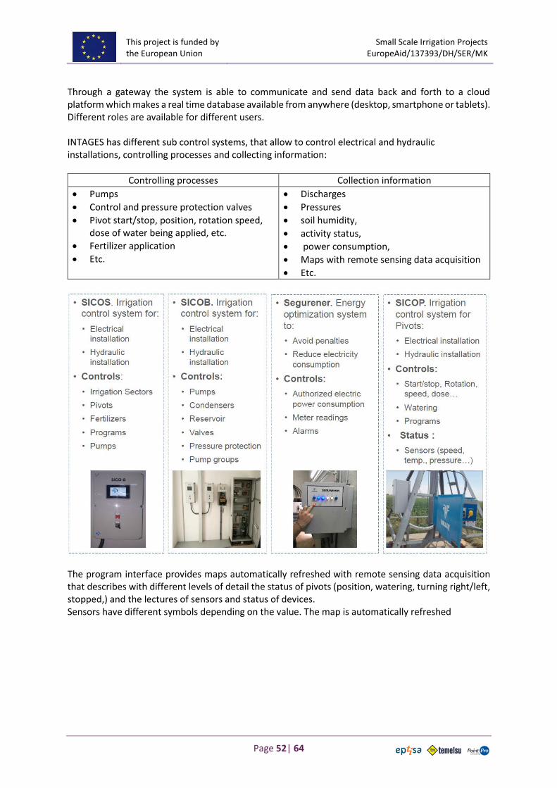
This project is funded by the European Union
Small Scale Irrigation Projects EuropeAid/137393/DH/SER/MK
Page 52| 64
Through a gateway the system is able to communicate and send data back and forth to a cloud platform which makes a real time database available from anywhere (desktop, smartphone or tablets). Different roles are available for different users. INTAGES has different sub control systems, that allow to control electrical and hydraulic installations, controlling processes and collecting information:
Controlling processes Collection information
• Pumps
• Control and pressure protection valves
• Pivot start/stop, position, rotation speed, dose of water being applied, etc.
• Fertilizer application
• Etc.
• Discharges
• Pressures
• soil humidity,
• activity status,
• power consumption,
• Maps with remote sensing data acquisition
• Etc.
The program interface provides maps automatically refreshed with remote sensing data acquisition that describes with different levels of detail the status of pivots (position, watering, turning right/left, stopped,) and the lectures of sensors and status of devices. Sensors have different symbols depending on the value. The map is automatically refreshed

This project is funded by the European Union
Small Scale Irrigation Projects EuropeAid/137393/DH/SER/MK
Page 53| 64
Beside the information showed in maps, there is also available scheme diagrams where the last available information synchronized with the more recent information from the Central Unit is shown: sensor data in boxes and symbols of different colors according to the value, and Alarm warnings.
For each pivot: position,
crops and status (watering,
turning right/left, stopped…)
Table of Contents and
Legend depends on the scale
(more elements when
zooming in)
Sensor: label and symbol
depends on the value. Click
on a sensor or device to get
more details: Valve closed.

This project is funded by the European Union
Small Scale Irrigation Projects EuropeAid/137393/DH/SER/MK
Page 54| 64
Analysis of historical data is available displayed with charts:
Training Material prepared by Oscar Coronel Irrigation Expert

This project is funded by the European Union
Small Scale Irrigation Projects EuropeAid/137393/DH/SER/MK
Page 55| 64
6 BIBLIOGRAPHY
Reference Description
Allen et al, 1998
Allen, R.G., Pereira, L.S., Raes, D. & Smith, M. Crop evapotranspiration. Guidelines for computing crop water requirements. FAO Irrigation and Drainage Paper No. 56. Rome, 1998.
Brouwer & Heibloem, 1986
C. Brouwer and M. Heibloem. IRRIGATION WATER MANAGEMEN: Irrigation Water Needs. Training manual no. 3. Food and Agriculture Organization of the United Nations, Rome, Italy, 1986
Doorenbos and Kassam,1979
Doorenbos J. and Kassam A.H. Yield Response to Water FAO IRRIGATION AND DRAINAGE PAPER 33. FOOD AND AGRICULTURE ORGANIZATION OF THE UNITED NATIONS, Rome, 1979
Doorenbos and Pruitt, 1977 Doorenbos, J. & Pruitt, W.O. Crop water requirements. FAO Irrigation and Drainage Paper No. 24. Rome, 1977
Smith, 1992 Smith, M. CROPWAT. A computer programme for irrigation planning and management. FAO Irrigation and Drainage Paper No. 46. Rome, FAO,1992
Smith, 1993 Smith M. CLIMWAT for CROPWAT. FAO Irrigation and Drainage Paper No. 49. Rome, FAO. 1993
Steduto et al,2012
Pasquale Steduto, Theodore C. Hsiao, Elias Fereres, Dirk Raes. Crop yield response to water FAO IRRIGATION AND DRAINAGE PAPER 66. FOOD AND AGRICULTURE ORGANIZATION OF THE UNITED NATIONS, Rome, 2012
Walker, 2003 Wynn R. Walker. SIRMOD III Surface Irrigation Simulation, Evaluation and Design Guide and Technical Documentation. Utah State University 2003

This project is funded by the European Union
Small Scale Irrigation Projects EuropeAid/137393/DH/SER/MK
Page 56| 64
7 ANNEXES
7.1 ANNEX I: EVALUATION OF IRRIGATION PERFORMANCE
This section describes how to determine the performance of basin/furrow irrigation. It is assumed that the net irrigation water need of the crop is known (i.e. the net irrigation depth). This is compared with what happens during the actual irrigation practice. The field application efficiency thus obtained is a good measure for the evaluation of the performance.
Figure 7-1 Place wooden posts at 5 a interval
Equipment needed - Measuring tape (30 m) - Infiltrometer - Wooden posts or lathes - Stopwatch or clock - Data sheet Method Step 1: Identify a typical basin or furrow, which can be considered representative of the local situation in terms of size, soil type and crop. Measure the basin size or furrow length with the tape. Record the site data on the data sheet: Example: Date of test: 4 December 1987 Basin size: 24 (m) x 15 (m) - 360 (m2) Crop: Groundnuts Required net irrigation depth: 45 mm Step 2: Place wooden posts at 5 to 10 m intervals as shown in Figure 4.3. Record position of the posts on the data sheet (column 2). Step 3: Carry out several infiltration tests (see Annex 3) and make an (average) infiltration curve. In this example, the curve of Annex 3 (Figure 76) is used. Step 4: Now the irrigation starts. Use the same stream size and the same irrigation time as the irrigator normally uses. Record the time it takes for the water front to reach each wooden post (1 to 6). This is called the advance time: column 3.

This project is funded by the European Union
Small Scale Irrigation Projects EuropeAid/137393/DH/SER/MK
Page 57| 64
Step 5: Record the time it takes the water to infiltrate at each wooden post (1 to 6). This is called recession time: column 4. Step 6: Calculate the contact time at each of the wooden posts. The contact time is the difference between the advance and recession time: column 5. Step 7: Calculate at each of the wooden posts the amount of water applied (in column 6 of the following table), using the infiltration curve. All data are recorded on the data sheet as indicated in the example below.
Step 8: Determine the field application efficiency. The field application efficiency is the fraction of the applied water that is used by the crop. Provided there are no runoff losses, the field application efficiency (%) is the required irrigation depth (mm), divided by the average applied irrigation depth (mm), multiplied by 100%. Or:
: The average irrigation depth applied (column 6) is: (65 + 63 + 61 + 60 + 56 + 46):6 = 59 mm The required net irrigation depth is 45 mm. Thus the field application efficiency (%) = 45/59 x 100% = 76% It means that the (average) deep percolation losses are 59 - 45 = 14 mm. This is shown in next table

This project is funded by the European Union
Small Scale Irrigation Projects EuropeAid/137393/DH/SER/MK
Page 58| 64
7.2 ANNEX 2 METEOROLOGICAL DATA FROM METEOROLOGICAL STATIONS KICHEVO, KRIVA PALANCA AND STRUMICA
Meteorological Station Kichevo
Monthly rainfall (sum) with various empirical probabilities of occurrence (25%, 50%, 75%)
P (mm) Jan Feb Mar Apr May Jun Jul Aug Sep Oct Nov Dec Sum
min 1,8 6,1 9,1 9,3 8,2 4,7 1 0,4 5 1,1 12,9 9,4 69
25% 37,8 36,4 45,2 38,75 29,58 27,88 14,6 17 23 37,45 56,3 57,3 421,3
50% 74,4 54,2 62,6 50,1 60,15 35,65 32,1 28 42,6 62,3 89,4 87,5 679
75% 124,2 70 102,7 69,15 79,65 65,18 55,4 48,4 58,9 118,4 123,6 117,6 1033,1
max 213,5 245,1 147,3 111,3 152,3 121 207,6 128,3 162,9 189,1 318,3 239,6 2236,3
Average temperature (°C) with various empirical probabilities of occurrence (25%, 50%, 75%)
T(°C) Jan Feb Mar Apr May Jun Jul Aug Sep Oct Nov Dec Av.
min -3,7 -3,1 1,5 8,5 12,4 16,6 19 17 14 7,5 0,2 -1,4 7,4
25% -1,5 1 5,2 9,8 14 18 20,1 19,8 15,8 10,5 5 0,8 9,9
50% 0,6 2,3 6,2 10,8 15,4 18,7 20,7 20,7 16,8 11,4 6,4 1,8 11
75% 1,6 3,8 7,4 12 16,3 19,2 21,6 21,3 17,3 12,4 7,6 2,8 11,9
max 4,6 6,8 9,3 13,2 18,9 21,5 24 23,5 19,1 15,2 10 5,6 14,3
Relative humidity (%) with various empirical probabilities of occurrence (25%, 50%, 75%)
RH (%) Jan Feb Mar Apr May Jun Jul Aug Sep Oct Nov Dec Av.
min 79 72 59 61 56 57 52 53 58 66 73 74 63,3
25% 83 78 69 65,3 66 64 60,3 59,5 66,3 72,3 77,3 83 70,3
50% 84,8 80 73,5 67,7 68,8 67 63 66,2 72 76,1 80,6 84,2 73,7

This project is funded by the European Union
Small Scale Irrigation Projects EuropeAid/137393/DH/SER/MK
Page 59| 64
75% 86 83,3 76,8 69,8 71 69 69,8 69,8 75,8 79,8 83 86,8 76,7
max 90 88 82 75 77 77 76 76 82 85 87 92 82,3
Wind speed (m/s) with various empirical probabilities of occurrence (25%, 50%, 75%)
WS (m/s) Jan Feb Mar Apr May Jun Jul Aug Sep Oct Nov Dec Av.
min 0,5 0,7 0,2 0,6 0,6 0,3 0,4 0,1 0,2 0,2 0,4 0 0,4
25% 1,6 1,5 1,8 1,5 1,5 1,4 1,6 1,4 1,2 1,3 1,5 1,5 1,5
50% 1,8 2 2,2 2,3 2 2,1 1,9 1,9 1,6 1,7 1,7 1,8 1,9
75% 2 2,3 2,6 2,5 2,2 2,3 2,3 2,1 2 2 2,2 2,1 2,2
max 4 4,5 5,6 4,6 4,8 3,9 3,5 4 2,8 2,8 3,1 3,5 3,9
Sunny hours (h) with various empirical probabilities of occurrence (25%, 50%, 75%)
SR (h) Jan Feb Mar Apr May Jun Jul Aug Sep Oct Nov Dec Sum
min 25,2 38,5 75,9 111,7 139,8 218,4 236,4 236,4 146,5 106,8 59,6 33,7 1428,9
25% 54,1 83,5 130,6 160,2 217,2 256,6 285 282,5 196,3 148,1 85,8 48,4 1948,2
50% 81,2 104 155 182,5 239,9 277,6 310,5 297,1 220,3 166,9 95,2 68,2 2198,2
75% 99,8 133,7 175,3 206,9 259 293,1 336,5 314 233,7 190,6 110 81,3 2433,8
max 174,2 183,6 222,8 245 297,2 330,3 389,3 348,4 300 260 166 129,1 3045,9

This project is funded by the European Union
Small Scale Irrigation Projects EuropeAid/137393/DH/SER/MK
Page 60| 64
Meteorological Station Kriva Palanca
Monthly rainfall (sum) with various empirical probabilities of occurrence (25%, 50%, 75%)
P (mm) Jan Feb Mar Apr May Jun Jul Aug Sep Oct Nov Dec Sum
min 1,3 3,3 0,4 4 23,4 13,1 0,3 5,6 4,4 0,4 0,2 10,1 66,5
25% 22,3 20,8 27,1 33,4 42,4 44,2 27 31,6 18,7 22,2 34,9 32,2 356,4
50% 36,4 34,2 45,6 48,9 65,6 60,7 46,2 40,3 36,3 46 51,1 50,4 561,7
75% 58,3 57,2 62,1 73,7 90,3 92,5 65,1 62,8 74,5 72 80,2 70,6 858,9
max 98 104,9 138,5 174,6 145,5 175,1 186,1 157,6 157,2 146,4 139,8 117,6 1741,3
Average temperature (°C) with various empirical probabilities of occurrence (25%, 50%, 75%)
T(°C) Jan Feb Mar Apr May Jun Jul Aug Sep Oct Nov Dec Av.
min -3,7 -4 0,2 4,9 10,9 15,2 17,8 15,2 13 6,9 -0,6 -4 5,9
25% -1,4 0,2 4 8,9 13,7 17,5 19,4 18,8 14,8 10 4,8 0,5 9,2
50% 0,4 1,8 5,2 9,8 14,8 18 20,1 19,9 15,9 10,7 6,1 1,5 10,35
75% 1,3 2,9 6,4 10,8 15,6 18,9 21,2 21,3 16,7 11,8 7,4 2,5 11,4
max 3,7 6,3 9,7 12,8 17,9 20,6 23,6 22,7 19,6 14,6 10,2 4,2 13,8
Relative humidity (%) with various empirical probabilities of occurrence (25%, 50%, 75%)
RH (%) Jan Feb Mar Apr May Jun Jul Aug Sep Oct Nov Dec Av.
min 70 62 54 52 52 52 51 47 52 58 65 70 57,1
25% 74,3 70,3 65 61 63 63 55,3 57 62,3 68 73 75,3 65,6
50% 76 73 68 63,5 67,5 66 60,5 61 66 71,6 76 77,9 68,9
75% 78 75 70 67,8 70 68 67 65 71,8 75,8 78 80 72,2
max 84 84 77 73 74 73 72 75 79 79 82 86 78,2

This project is funded by the European Union
Small Scale Irrigation Projects EuropeAid/137393/DH/SER/MK
Page 61| 64
Wind speed (m/s) with various empirical probabilities of occurrence (25%, 50%, 75%)
WS (m/s) Jan Feb Mar Apr May Jun Jul Aug Sep Oct Nov Dec Av.
min 1,6 1,8 1,8 1,9 1,5 1,5 1,7 1,9 1,9 0,8 0,9 1 1,5
25% 2,2 2,2 2,3 2,3 2,2 2,1 2,2 2,2 2,3 2,3 2,2 2,1 2,2
50% 2,5 2,7 2,8 2,7 2,5 2,4 2,7 2,8 2,9 3 2,6 2,4 2,6
75% 3 3,4 3,5 3,3 3,1 3,2 3,3 3,5 3,6 3,6 3,3 3 3,3
max 4,3 4,2 4,5 4,2 4,2 3,9 4 4,1 4,2 4,4 4,4 4 4,2
Sunny hours (h) with various empirical probabilities of occurrence (25%, 50%, 75%)
SR (h) Jan Feb Mar Apr May Jun Jul Aug Sep Oct Nov Dec Sum
min 43,1 46,7 94,8 120,4 149,6 191,1 232,5 215,6 130,4 116,7 63 0 1403,9
25% 74,1 100,2 117,3 155,6 209,3 244,8 285,8 271,8 198,7 160 101,4 67,5 1986,2
50% 97,6 118,9 162,1 172,1 224,9 267,4 305,5 304,4 221,2 187,8 123,8 81,9 2267,3
75% 127,3 142,8 183,3 203,8 253 288,8 337,6 323,3 248,4 209,3 137,4 105,3 2560,4
max 158,9 188,1 225,7 272,5 304,3 365,3 383,9 356 307,9 262,5 174,7 141,1 3140,9

This project is funded by the European Union
Small Scale Irrigation Projects EuropeAid/137393/DH/SER/MK
Page 62| 64
Meteorological Station Strumica
Monthly rainfall (sum) with various empirical probabilities of occurrence (25%, 50%, 75%)
P (mm) Jan Feb Mar Apr May Jun Jul Aug Sep Oct Nov Dec Sum
min 0,3 0,3 2,6 2,2 4,4 4,3 0 0,7 0,5 0 7,5 5,2 28
25% 22,95 19,1 23,35 27,95 35,8 26,8 11,45 11,55 13,65 28,2 30,3 36,85 288
50% 38,9 39,9 40,3 41,7 53,6 40,1 22,9 27,2 31 52,8 51,9 56,6 496,9
75% 59,45 58,2 57,8 64,6 79,75 60,65 43,95 55,45 62 77,3 83,5 87,55 790,2
max 94,1 169,9 126 125,5 155,8 156,5 179 101 189,7 195,9 173 228,3 1894,7
Average max. temperature (°C) with various empirical probabilities of occurrence (25%, 50%, 75%)
T(°C) Jan Feb Mar Apr May Jun Jul Aug Sep Oct Nov Dec Av.
min 1,2 2,5 8,4 14,2 20,2 25,6 28,7 25,7 22,5 15,2 6,4 -0,7 14,2
25% 4,2 7,7 12,6 18,1 22,8 27,8 30,2 29,6 26 19,5 11,7 5,8 18
50% 5,8 9,1 14,3 19,3 25 28,5 31 30,9 27 20,2 13,2 7 19,3
75% 7,2 10,9 16 20,1 25,6 29,8 32 32,7 27,8 21,2 14,1 8,1 20,5
max 12,5 14,9 19,6 22,8 27,9 31,4 35,5 35 34,2 24,3 18,3 9,8 23,9
Average min. temperature (°C) with various empirical probabilities of occurrence (25%, 50%, 75%)
T(°C) Jan Feb Mar Apr May Jun Jul Aug Sep Oct Nov Dec Av.
min -10,1 -10 -4,7 2,1 8 11,3 13,2 12,1 8,7 3,4 -2,4 -9,2 1,9
25% -4,1 -2,3 0,9 5,1 9,6 13,3 14,4 14,1 10,2 5,4 1,2 -2,2 5,5
50% -2,5 -0,6 2,2 5,7 10,3 13,8 15,3 14,7 11,2 7,4 2,9 -0,7 6,6
75% -0,5 0,9 3,1 6,7 11,1 14,4 16,2 15,9 12 8 4,2 0,3 7,7
max 2,1 2,8 4,7 8,2 12,9 16,1 17,5 18,3 13,6 10,4 7,2 2,7 9,7

This project is funded by the European Union
Small Scale Irrigation Projects EuropeAid/137393/DH/SER/MK
Page 63| 64
Average temperature (°C) with various empirical probabilities of occurrence (25%, 50%, 75%)
T(°C) Jan Feb Mar Apr May Jun Jul Aug Sep Oct Nov Dec Av.
min -5,1 -1,7 3,3 7,9 14,3 19,4 21,7 19,2 15,8 9,8 1,3 -4,7 8,4
25% -0,3 2,4 7,1 12,1 16,9 21,4 23 22,4 18 11,9 6,4 1,7 11,9
50% 1,3 4 8,2 12,9 18 21,9 24,1 23,4 19,1 13,2 7,5 2,8 13
75% 2,9 5,4 9,3 13,7 18,8 22,7 25 24,8 20 13,8 8,7 3,9 14,1
max 5,3 8,9 11,9 15,8 21,6 24,6 27,7 26,9 22,8 17,4 11,6 5,9 16,7
Relative humidity (%) with various empirical probabilities of occurrence (25%, 50%, 75%)
RH (%) Jan Feb Mar Apr May Jun Jul Aug Sep Oct Nov Dec Av.
min 74 66 57 55 53 46 41 42 54 64 69 80 58,4
25% 83 75 69 64,3 64 60 53,5 57,3 64,3 73 81 84 69
50% 85 79,2 73 70 68 62,5 58,7 62 68,4 76,5 83 86,2 72,7
75% 88 83 78 74 72 65,8 64 66 73,8 80,8 86 88,8 76,7
max 92 93 88 82 79 82 75 76 82 86 91 97 85,3
Wind speed (m/s) with various empirical probabilities of occurrence (25%, 50%, 75%)
WS (m/s) Jan Feb Mar Apr May Jun Jul Aug Sep Oct Nov Dec Av.
min 0,2 0,4 0,7 0,6 0,3 0,6 0,3 0,2 0,3 0,3 0,2 0,1 0,4
25% 0,6 1 1,2 1,2 0,9 0,9 0,8 0,6 0,6 0,4 0,4 0,5 0,8
50% 1 1,2 1,6 1,4 1,3 1,2 1,1 1 1 0,7 0,8 0,8 1,1
75% 1,2 1,6 1,9 1,7 1,5 1,4 1,3 1,2 1,2 0,9 1 1 1,3
max 2,2 2,4 3 2,9 1,9 2 1,9 1,5 1,5 1,2 1,6 1,6 2
Sunny hours (h) with various empirical probabilities of occurrence (25%, 50%, 75%)
SR (h) Jan Feb Mar Apr May Jun Jul Aug Sep Oct Nov Dec Sum

This project is funded by the European Union
Small Scale Irrigation Projects EuropeAid/137393/DH/SER/MK
Page 64| 64
min 19,6 25,9 66,8 125,2 154,4 206,7 212,5 246,8 133,9 98,5 56,6 14,8 1362
25% 65,6 96,3 139,9 168,9 229,8 272,2 316,3 290,3 206,1 158 94,1 65,9 2103
50% 89,2 117,7 159,5 190,1 246,7 285,5 332,8 308,2 230,7 176,6 108,5 78,2 2324
75% 108,2 138,1 184,5 206 259,9 303,3 358,6 325,6 250,8 193,6 125,8 88,8 2543
max 168,3 187,1 253,9 271,1 315,2 383,9 394,7 364,4 291,9 230,6 164,7 142,3 3168