Training course: boundary layer; surface layer Parametrization of surface fluxes: Outline Surface...
39
training course: boundary layer; surface layer Parametrization of surface fluxes: Outline • Surface layer (Monin Obukhov) similarity • Surface fluxes: Alternative formulations • Roughness length over land – Definition – Orographic contribution – Roughness lengths for heat and moisture • Ocean surface fluxes – Roughness lengths and transfer coefficients – Low wind speeds and the limit of free convection – Air-sea coupling at low wind speeds: Impact
-
Upload
arianna-stevens -
Category
Documents
-
view
218 -
download
1
Transcript of Training course: boundary layer; surface layer Parametrization of surface fluxes: Outline Surface...

training course: boundary layer; surface layer
Parametrization of surface fluxes: Outline
• Surface layer (Monin Obukhov) similarity
• Surface fluxes: Alternative formulations
• Roughness length over land– Definition
– Orographic contribution
– Roughness lengths for heat and moisture
• Ocean surface fluxes– Roughness lengths and transfer coefficients
– Low wind speeds and the limit of free convection
– Air-sea coupling at low wind speeds: Impact

training course: boundary layer; surface layer
Mixing across steep gradients
Stable BL Dry mixed layer
Cloudy BL
Surface flux parametrization is sensitive because of large
gradients near the surface.
training course: boundary layer; surface layer
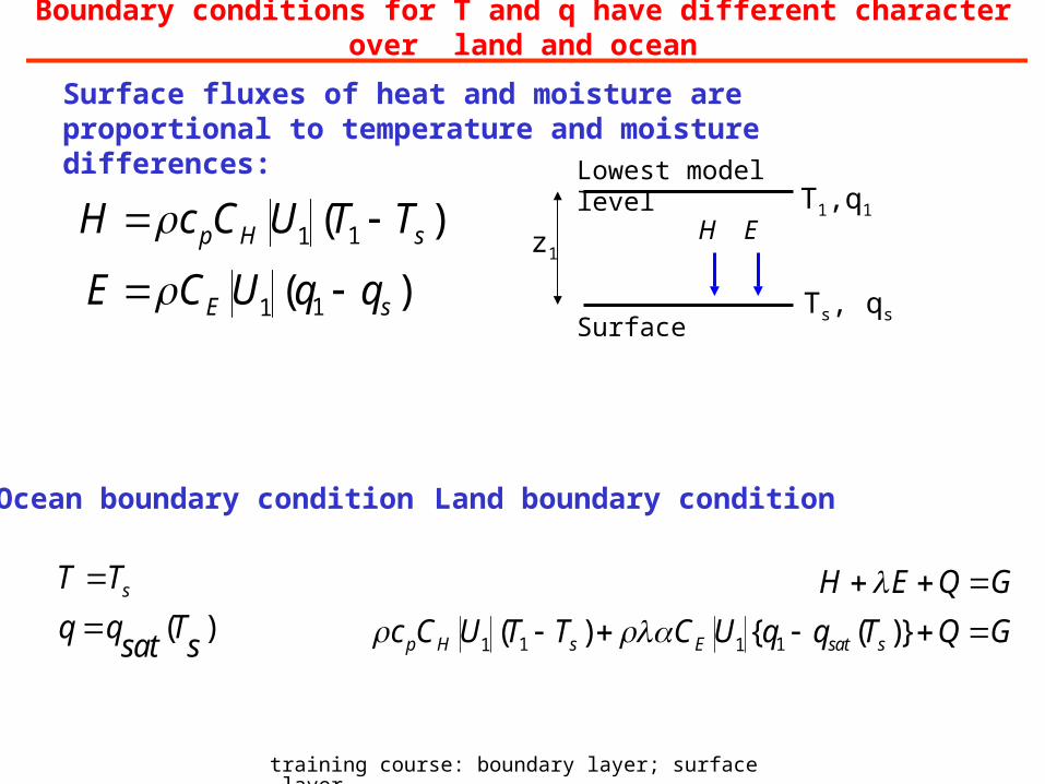
Boundary conditions for T and q have different character over land and ocean
Surface fluxes of heat and moisture are proportional to temperature and moisture differences:
T1,q1
Lowest model level
SurfaceTs, qs
z1H E11
11
( )
( )
p H s
E s
H c C U T T
E C U q q
Ocean boundary condition Land boundary condition
( )sT T
q q Tsat s
1 11 1( ) { ( )}p H s E sat s
H E Q G
c C U T T C U q q T Q G

training course: boundary layer; surface layer
Parametrization of surface fluxes: Outline
• Surface layer (Monin Obukhov) similarity
• Surface fluxes: Alternative formulations
• Roughness length over land– Definition
– Orographic contribution
– Roughness lengths for heat and moisture
• Ocean surface fluxes– Roughness lengths and transfer coefficients
– Low wind speeds and the limit of free convection
– Air-sea coupling at low wind speeds: Impact
training course: boundary layer; surface layer
h
.surf
Flux profile
layersurface0 o
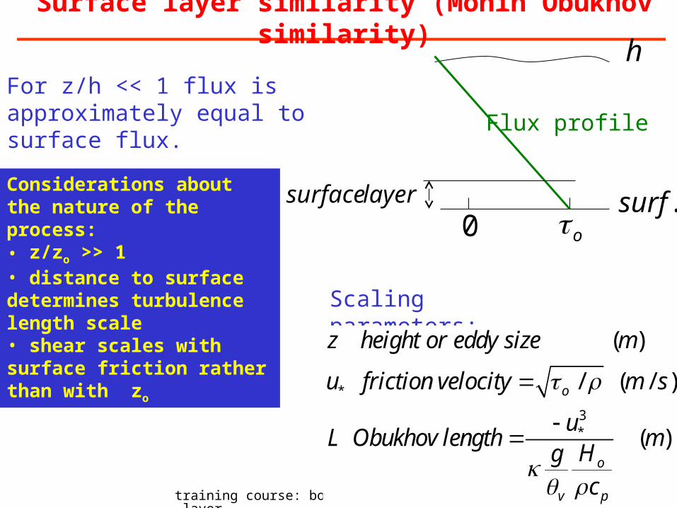
For z/h << 1 flux is approximately equal to surface flux.
Scaling parameters:
*
3*
( )
/ ( / )
( )
o
o
v p
z height or eddy size m
u friction velocity m s
uL Obukhov length m
Hgc
Surface layer similarity (Monin Obukhov similarity)
Considerations about the nature of the process:• z/zo >> 1• distance to surface determines turbulence length scale• shear scales with surface friction rather than with zo

training course: boundary layer; surface layer
MO similarity for gradients
*h
z
z
z
L
*m
U z
z u
dimensionless shear
Stability parameter
z
L
(von Karman constant) is defined such that 1 for / 0m z L
dimensionless potential temperature gradient
Stability parameter
*h
z
z
z
L
is a universal function of
is a universal function of
1
' 'm
UK u w
z
*
1m
m
K
zu Note that with we obtain:
training course: boundary layer; surface layer
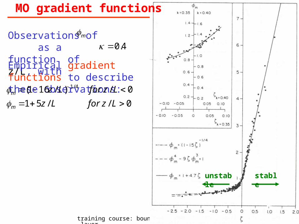
Observations of as a function of z/L, with
m4.0
Empirical gradient functions to describe these observations:
0//51
0/)/161( 4/1
LzforLz
LzforLz
m
m
stableunstable
MO gradient functions

training course: boundary layer; surface layer
Parametrization of surface fluxes: Outline
• Surface layer (Monin Obukhov) similarity
• Surface fluxes: Alternative formulations
• Roughness length over land– Definition
– Orographic contribution
– Roughness lengths for heat and moisture
• Ocean surface fluxes– Roughness lengths and transfer coefficients
– Low wind speeds and the limit of free convection
– Air-sea coupling at low wind speeds: Impact
training course: boundary layer; surface layer
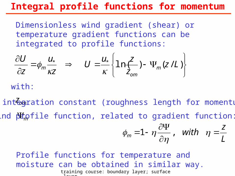
Integral profile functions for momentum
Dimensionless wind gradient (shear) or temperature gradient functions can be integrated to profile functions:
)/()ln(** Lzz
zuU
z
u
z
Um
omm
with:
omz integration constant (roughness length for momentum)
m wind profile function, related to gradient function:
L
zwithm
,1
Profile functions for temperature and moisture can be obtained in similar way.

training course: boundary layer; surface layer
Integral profile functions: Momentum, heat and moisture
Profile functions for surface layer applied between surface and lowest model level provide link between fluxes and wind, temperature and moisture differences.
11 1
*
11 1
*
11 1
*
11 1
*
{ln( ) ( / )}
{ln( ) ( / )}
{ln( ) ( / )}
{ln( ) ( / )}
xom
om
yom
om
s hp oh
s h
om
om
om
om
oq
zU z L
u z
zV z L
u
z
z
z
z
zHz L
c u z
zEq
zq z L
u z
00 Displacement height: Numerically necessary for large values of mz z

training course: boundary layer; surface layer
MO wind profile functions applied to observations
Stable Unstable

training course: boundary layer; surface layer
Transfer coefficients
Surface fluxes can be written explicitly as:
U1,V1,T1,q1
Lowest model level
Surface0, 0, Ts, qs
z1x y H E
11
11
11
11
( )
( )
x M
y M
p H s
E s
C U U
C U V
H c C U
E C U q q
1/ 22 21 11where U U V
2
1 1 1 1
and{ln( / ) ( / )}{ln( / ) ( / )}om m o
kC
z z z L z z z L
M
H
E
m
h
q
m
h
h

training course: boundary layer; surface layer
Numerical procedure: The Richardson number
The expressions for surface fluxes are implicit i.e they contain the Obukhov length which depends on fluxes. The stability parameter z/L can be computed from the bulk Richardson number by solving the following relation:
211
1112
1
11
)}/()/{ln(
)}/()/{ln(
|| Lzzz
Lzzz
L
z
U
gzRi
mom
hohsb
This relation can be solved: •Iteratively;•Approximated with empirical functions; •Tabulated.

training course: boundary layer; surface layer
Louis scheme
1 1 11( ' ') ( ) ( , / , / )n s b om ow C U F Ri z z z z 2
1 1{ln( / )}{ln( / )}nom o
Cz z z z
The older Louis formulation uses:
With neutral transfer coefficient:
And empirical stability functions for 1 1( , / , / )b om oF Ri z z z z
( )u v
q
Initially, the empirical stability functions, , were not related to the (observed-based) Monin-Obukhov functions.
F
training course: boundary layer; surface layer
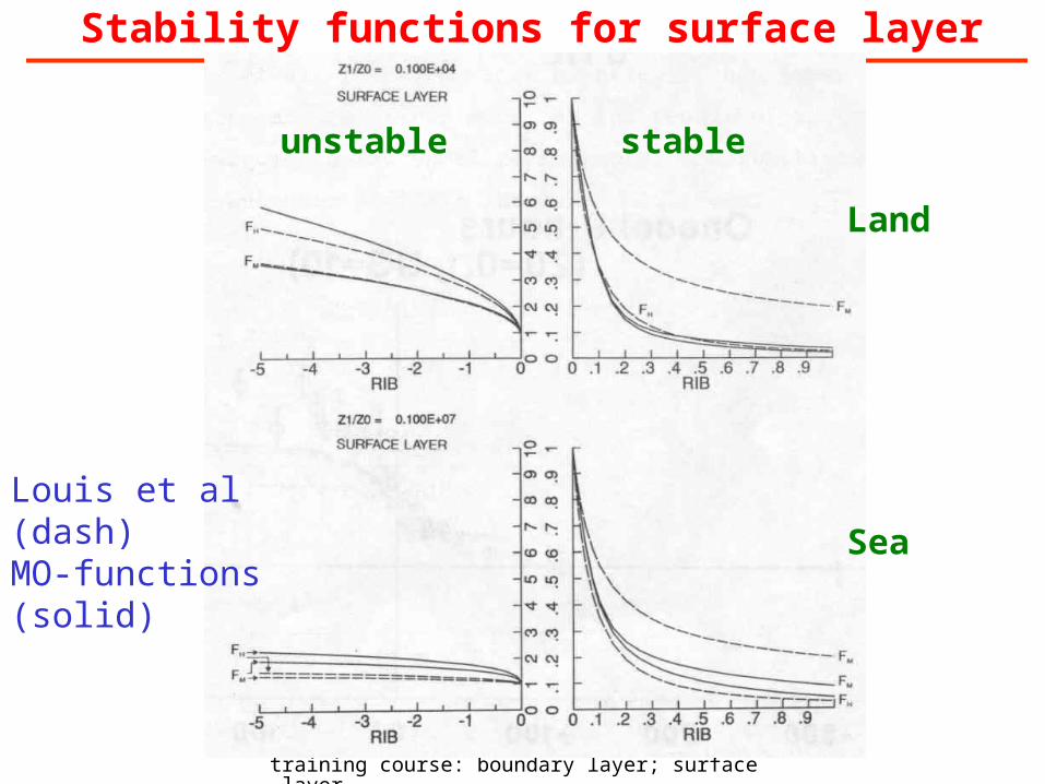
Stability functions for surface layer
Louis et al (dash)MO-functions (solid)
unstable stable
Land
Sea

training course: boundary layer; surface layer
Surface fluxes: Summary
11
2
1 1 1 1
1 1 1
112
1
( ' ')
{ln( / ) ( / )}{ln( / ) ( / )}
/ ( , / , / )
( )b
s
om m o
b om o
o
w C U
kC
z z z L z z z L
z L f Ri z z z z
g zRi
U
•MO-similarity provides solid basis for parametrization of surface fluxes:
•Different implementations are possible (z/L-functions, or Ri-functions) •Surface roughness lengths are crucial aspect of formulation.•Transfer coefficients are typically 0.001 over sea and 0.01 over land, mainly due to surface roughness.

training course: boundary layer; surface layer
Parametrization of surface fluxes: Outline
• Surface layer (Monin Obukhov) similarity
• Surface fluxes: Alternative formulations
• Roughness length over land– Definition
– Orographic contribution
– Roughness lengths for heat and moisture
• Ocean surface fluxes– Roughness lengths and transfer coefficients
– Low wind speeds and the limit of free convection
– Air-sea coupling at low wind speeds: Impact

training course: boundary layer; surface layer
Surface roughness length (definition)
•Surface roughness length is defined on the basis of logarithmic profile.•For z/L small, profiles are logarithmic.•Roughness length is defined by intersection with ordinate.
zln10
0.1
0.01
1
U
omz
Example for wind:
)ln(*
omz
zuU
)ln(*
om
om
z
zzuU
Often displacement height is used to obtain U=0 for z=0:
• Roughness lengths for momentum, heat and moisture are not the same.•Roughness lengths are surface properties.

training course: boundary layer; surface layer
Roughness length over land
Geographical fields based on land use tables:
Ice surface 0.0001 m
Short grass 0.01 m
Long grass 0.05 m
Pasture 0.20 m
Suburban housing 0.6 m
Forest, cities 1-5 m
training course: boundary layer; surface layer
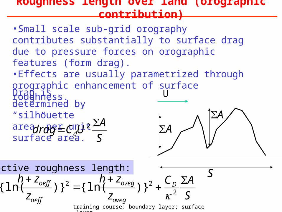
Roughness length over land (orographic contribution)
•Small scale sub-grid orography contributes substantially to surface drag due to pressure forces on orographic features (form drag). •Effects are usually parametrized through orographic enhancement of surface roughness.
Effective roughness length:
S
AC
z
zh
z
zhD
oveg
oveg
oeff
oeff
222 )}{ln()}{ln(
Drag is determined by “silhouette area” per unit surface area.
U
S
AUCdrag d
2 A
S
A

training course: boundary layer; surface layer
)(2 22mm
os hUC
Orographic form drag (simplified Wood and Mason, 1993):
Shape parametersDrag coefficientSilhouette slope Wind speedReference height m
m
h
U
C
,
mhzoso e /
Vertical distribution (Wood et al, 2001):
Roughness length over land (orographic contribution)

training course: boundary layer; surface layer
mhzm
m
mo ehUh
C
z/22 )(
2
Assume: khm /1~
dkkFkok
)(22
Write flux divergence as:
Parametrization of flux divergence with continuous orographic spectrum:
dkekcUkFkCz
o
m
k
czkmm
o
/23 )/()(2
100 m1000 m
Beljaars, Brown and Wood, 2003
training course: boundary layer; surface layer
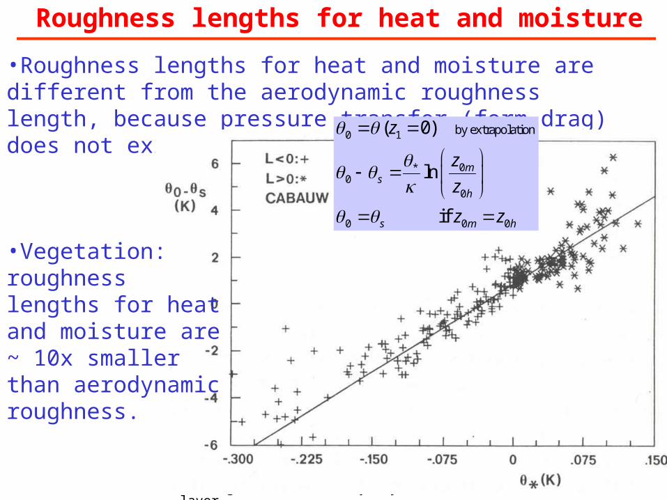
Roughness lengths for heat and moisture
•Roughness lengths for heat and moisture are different from the aerodynamic roughness length, because pressure transfer (form drag) does not exist for scalars.
•Vegetation: roughness lengths for heat and moisture are ~ 10x smaller than aerodynamic roughness.
0 1
0*0
0
0 0 0
by extrapolation( 0)
ln
if
ms
h
s m h
z
z
z
z z

training course: boundary layer; surface layer
Parametrization of surface fluxes: Outline
• Surface layer (Monin Obukhov) similarity
• Surface fluxes: Alternative formulations
• Roughness length over land– Definition
– Orographic contribution
– Roughness lengths for heat and moisture
• Ocean surface fluxes– Roughness lengths and transfer coefficients
– Low wind speeds and the limit of free convection
– Air-sea coupling at low wind speeds: Impact

training course: boundary layer; surface layer
Roughness lengths over the ocean
Roughness lengths are determined by molecular diffusion and ocean wave interaction e.g.
*
*
*
*
2
0.11 ,
0.40
0.62
ch
o
om
h
oq
ch C is Charnock parameteru
zu
zg
zu
uC
Current version of ECMWF model uses an ocean wave model to provide sea-state dependent Charnock parameter.

training course: boundary layer; surface layer
Transfer coefficents for moisture (10 m reference level)
**
2* 62.0,11.0018.0
uz
ug
uz oqom
omoqom zzug
uz ,11.0018.0
*
2*
•Using the same roughness length for momentum and moisture gives an overestimate of transfer coefficients at high wind speed
•The viscosity component increases the transfer at low wind speed
CE
N N
e utr
al e
x ch
ange
coe
ff f
or e
v ap
ora t
ion
training course: boundary layer; surface layer
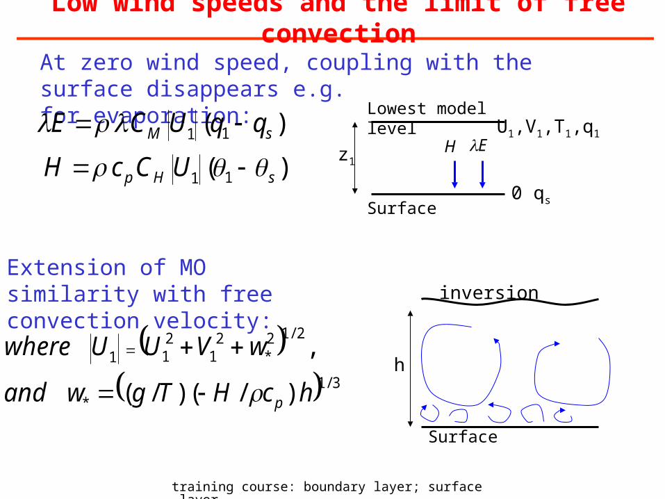
Low wind speeds and the limit of free convection
At zero wind speed, coupling with the surface disappears e.g. for evaporation:
U1,V1,T1,q1
Lowest model level
Surface0 qs
z1E
)( 11 sM qqUCE
3/1
*
2/12*
21
211
)/()/(
,
hcHTgwand
wVUUwhere
p
Surface
h
inversionExtension of MO similarity with free convection velocity:
)( 11 sHp UCcH H

training course: boundary layer; surface layer
Air-sea coupling at low winds
Revised scheme: Larger coupling at low wind speed (0-5 ms-1)
0 0m hz z

training course: boundary layer; surface layer
Air-sea coupling at low winds (control)
Precipitation, JJA; old formulation
training course: boundary layer; surface layer
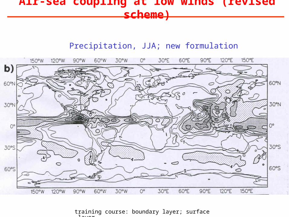
Air-sea coupling at low winds (revised scheme)
Precipitation, JJA; new formulation

training course: boundary layer; surface layer
Air-sea coupling at low winds
Near surface Theta_e difference: New-Old

training course: boundary layer; surface layer
Air-sea coupling at low winds
Theta and Theta_e profiles over warm pool with old an new formulation
new
old
new
old

training course: boundary layer; surface layer
Air-sea coupling at low winds
Zonal mean wind errors for DJF
Old
New
training course: boundary layer; surface layer
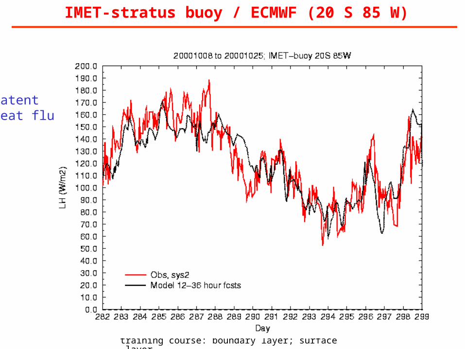
IMET-stratus buoy / ECMWF (20 S 85 W)
Latentheat flux
training course: boundary layer; surface layer
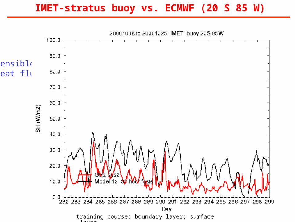
IMET-stratus buoy vs. ECMWF (20 S 85 W)
Sensibleheat flux

training course: boundary layer; surface layer
IMET-stratus buoy vs. ECMWF (20 S 85 W)
Horizontal wind speed

training course: boundary layer; surface layer
IMET-stratus buoy vs. ECMWF (20 S 85 W)
Water/air q-difference
training course: boundary layer; surface layer
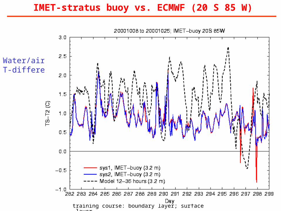
IMET-stratus buoy vs. ECMWF (20 S 85 W)
Water/air T-difference
training course: boundary layer; surface layer
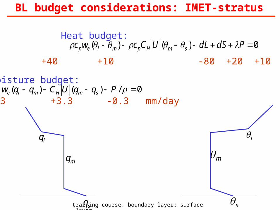
BL budget considerations: IMET-stratus
m
i
s
iq
sq
mq
0/)()( PqqUCqqw smHmie
0)()( PdSdLUCcwc smHpmiep
-3 +3.3 -0.3 mm/day
+40 +10 -80 +20 +10 W/m2
Moisture budget:
Heat budget: