Training and Optimization - cs.haifa.ac.il

Training and Optimization

Many slides from: Stanford CS231

1

• A network is represented using a computation graph.

• Our goal: learning the network parameters through

optimization.

Where are we now?

�

W1 b1

� ℒ

W2 b2

�ℎlossLinearLinear �(�)

2

Loop:

1. Sample a batch of data

2. Forward prop it through the graph (network), get loss

3. Backprop to calculate the gradients

4. Update the parameters using the gradient

Mini-batch SGD

�

W1 b1

� ℒ

W2 b2

�ℎlossLinearLinear �(�)

�� = − �� ℒ� �

�

�� 3

• One time setup:

activation functions, preprocessing, weight initialization,

regularization, gradient checking

• Training dynamics:

babysitting the learning process, parameter updates,

hyperparameter optimization

• Evaluation:

Bias vs. variance

Training and Optimization: Overview

Source: Stanford CS231

4

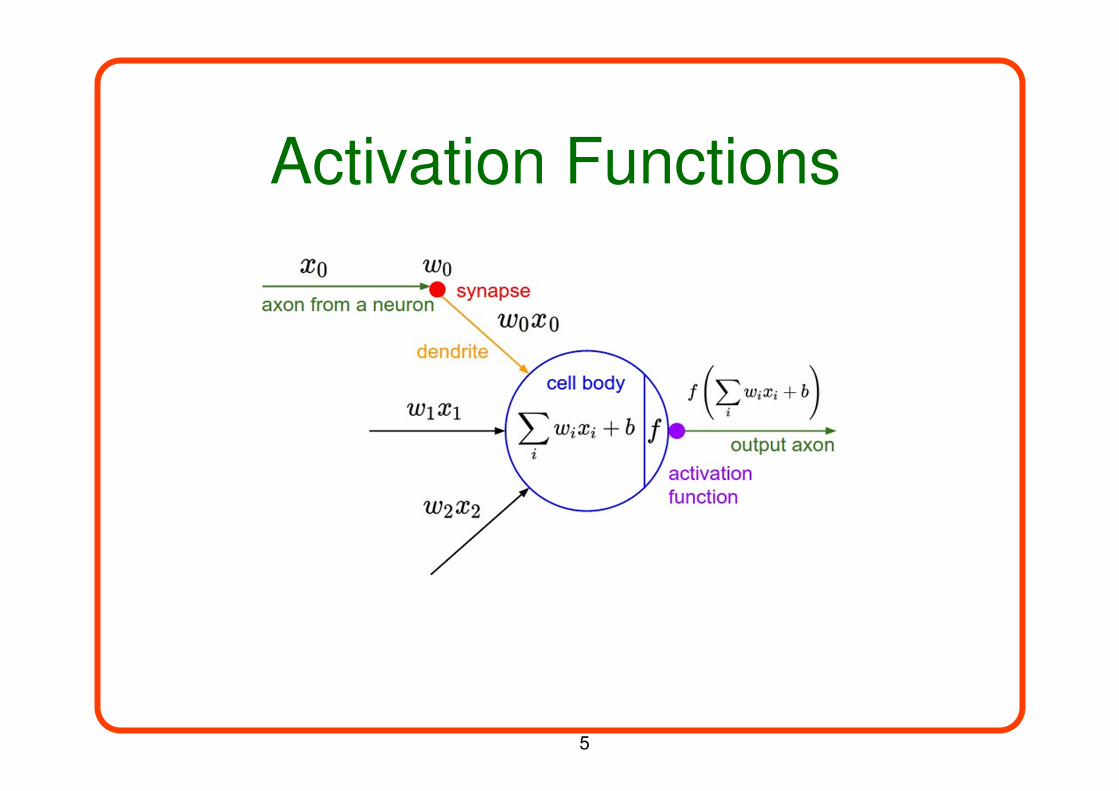
Activation Functions

5

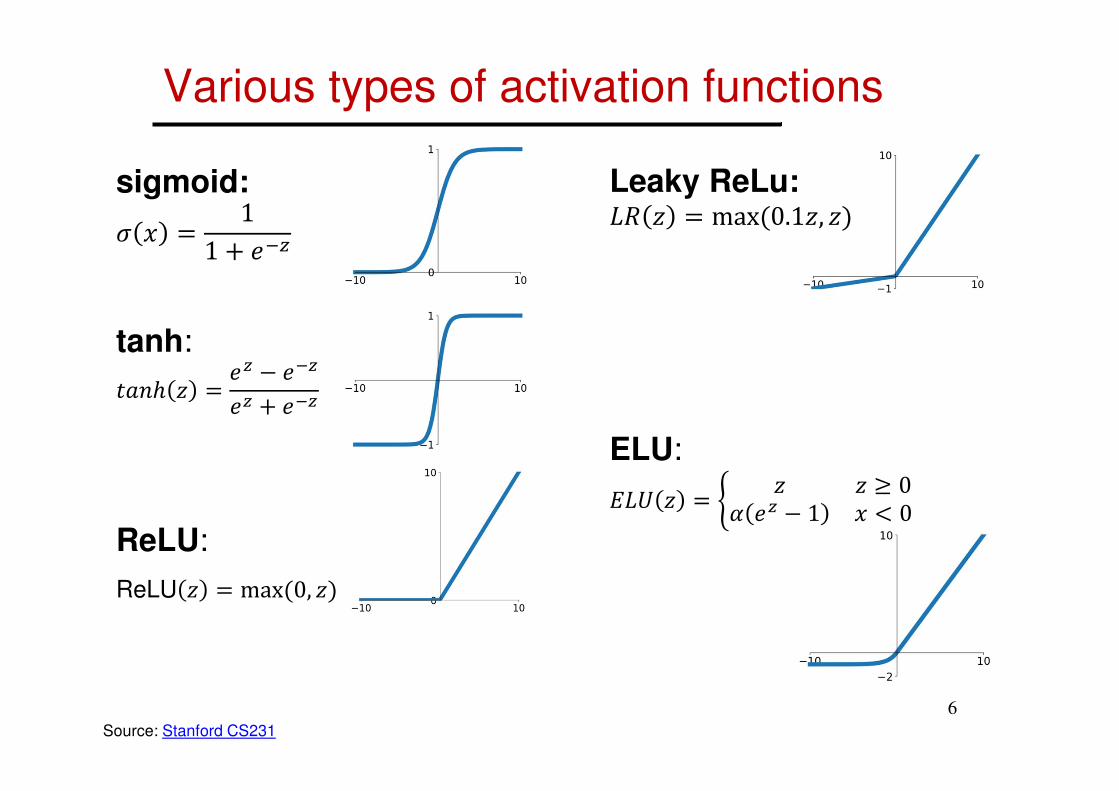
Various types of activation functions


sigmoid:

� � = 11 � ��

tanh:

��ℎ � ��

ReLU:

ReLU � max �0, ��

Leaky ReLu:%& � max �0.1�, ��

ELU:

(%) � * � � + 0, �� 1 � - 0

6

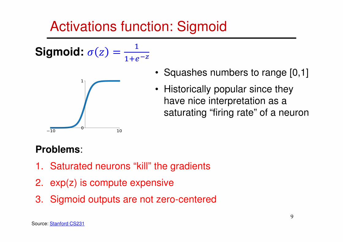
Sigmoid: � � ��./0

Activations function: Sigmoid


• Squashes numbers to range [0,1]

• Historically popular since they

have nice interpretation as a

saturating “firing rate” of a neuron

Problems:

1. Saturated neurons “kill” the gradients

7



• What happens when � �10 ?• What happens when � 0 ?• What happens when � 10 ?

sigmoid

gate��

� �

�ℒ��

�ℒ�� ℒ

��

8



• Squashes numbers to range [0,1]

• Historically popular since they

have nice interpretation as a

saturating “firing rate” of a neuron

Sigmoid: � � ��./0

Problems:

1. Saturated neurons “kill” the gradients

2. exp(z) is compute expensive

3. Sigmoid outputs are not zero-centered

9



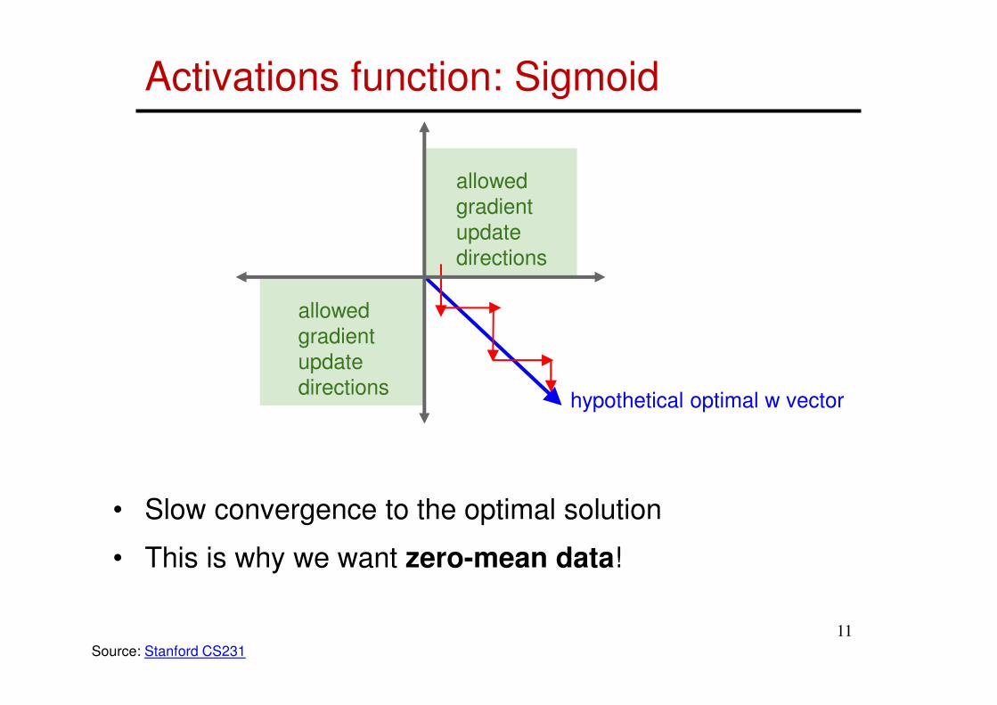
Sigmoid outputs are not zero-centered

• What happens to the gradients of 1 when the input to a

neuron is always positive?

• Answer: 2ℒ23 will be all positive or negative

• So, what is wrong with that?

4�56 � 7�

�ℒ�4

�ℒ�1 �ℒ

�4�4�1

, 7�4�1 48 � 6

10



• Slow convergence to the optimal solution

• This is why we want zero-mean data!

hypothetical optimal w vector

allowed

gradient

update

directions

allowed

gradient

update

directions

11

tanh:

Activations function: tanh


• Squashes numbers to range [-1,1]

• Zero-centered (nice)

• Still “kills” gradients when saturated (active in small range)

• Still exp(z) is compute expensive

��ℎ � ��

12

ReLU (Rectified Linear Unit):

Activations function: ReLU

• Does not saturate (in the � 9 0 region)

• Computationally very efficient

• Converges much faster than sigmoid/tanh (6x)

• Not zero-centered

• “Dead” parameter regions

:�;� max �<, ;�


13



“Dead” parameter regions

• What happens when � 10 ?• What happens when � 0 ?• What happens when � �10 ?

ReLU

gate��4��

4 � max�0, z�

�ℒ�4

�ℒ�� ℒ

�4�4��

14



DATA CLOUDactive ReLU

Dead ReLU

will never activate

never update 15

ReLU alternatives


• Does not saturate

• Computationally efficient

• Converges fast

• Will not “die”

• Related alternative: Parametric ReLU

4 � max ,�, � and backprop into ,

Leaky ReLU

4 � max 0.01�, �

16

ReLU alternatives


• All benefits of ReLU

• Does not die

• Close to zero mean outputs

• Computation requires exp()

Exponential Linear Units (ELU)

4 � * � >4 � 9 0, exp � � 1 � A 0

17

TDLR: Activation functions


• Use ReLU. Be careful with your learning rates

• Try out Leaky ReLU / ELU

• Try out tanh but don’t expect much

• Don’t use sigmoid

18

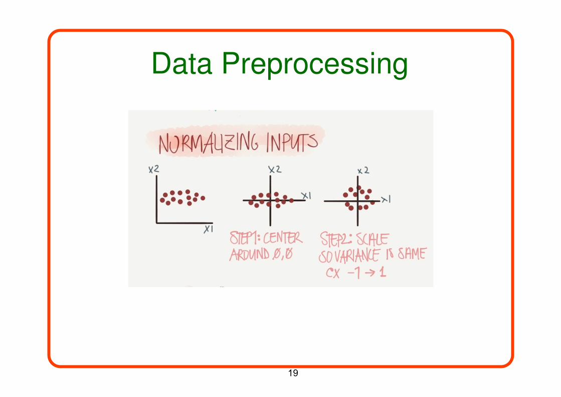
Data Preprocessing

19

• For a linear neuron with a squared

error, it is a quadratic bowl.

• Vertical cross-sections are parabolas.

• Horizontal cross-sections are ellipses.

• For multi-layer, non-linear nets the error

surface is much more complicated.

• But locally, a piece of a quadratic bowl

is usually a very good approximation.

Data preprocessing

Source: Geoffrey Hinton

Reminder: The error surface for a linear neuron

20

Data preprocessing


• Going downhill reduces the error, but the direction of

steepest descent does not point at the optimal point unless

the ellipse is a circle.

• The gradient is big in the direction in which we only want to

travel a small distance.

• The gradient is small in the direction in which we want to

travel a large distance.

• This produces zig-zag path.

21

Zero centering


• When using steepest descent, shifting the input values

makes a big difference.

• It usually helps to transform each component of the input

vector so that it has zero mean over the whole training set.

�� B �101 101 2101 99 2

�� B �1 1 21 �1 2

gives error surface

gives error surface�� B

Scaling


• When using steepest descent, scaling the input values

makes a big difference.

• It usually helps to transform each component of the input

vector so that it has unit variance over the whole training set.

�� B �0.1 10 20.1 �10 2

�� B �1 1 21 �1 2

gives error surface

gives error surface�� B

Data preprocessing

(Assume X [NxD] is a data matrix, each example in a row)

�� E��


24

Data preprocessing


(data has diagonal

covariance matrix)

(covariance matrix is

the identity matrix)

• In practice, you may also see PCA and Whitening of the

data.

• This can be performed using SVD:

X ← H �I�� H, ��>J 0 , ), K, L JMN H , H3O�. K��/B)5H• For linear neuron, this converts the data to be uncorrelated.

Data preprocessing

Data preprocessing for images:

• Subtract the mean image (all input images need to have

the same resolution).

• Subtract per-channel means (images don’t need to

have the same resolution).

• Be sure to apply the same transformation at training and

test time! Save training set statistics and apply to test

data.

• Not common to normalize variance, or to apply PCA or

whitening (why).

26

Weight Initialization

27

Weight initialization:

• What’s wrong with initializing all weights to be the same

number (e.g. zero)?

• If two hidden units have exactly the same incoming and

outgoing weights, they will always get exactly the same

values.

• The gradients is also the same for every unit, thus, all

the weights have the same values in the subsequent

iterations.

1�

1B

possible weights

Weight initialization: Experiments

• Initiate the weights with small random numbers (Gaussian with zero mean and � standard deviation): 1 ~R�0, ��


HD

W σ ∗ np. random. randn�D, H�

29


• 10-layer network

• 10 neurons on each layer

• tanh non-linearities

• Iinitialized by randn


Recall: For two independent random variables:M�\ �� M�\ � M�\ � � (B � M�\ � � (B � M�\ � M�\ � � � M�\ � � M�\ � ; M�\ �� B M�\ � ,

First try: Initiate the weights with zero mean Gaussian

values with 1E-2 standard deviation.


All activations

become zero!

Q: think about the

backward pass.

What do the

gradients look like?

Hint: think about

backward pass for

a ^� gate.


31

Second try: Initiate the weights with zero mean Gaussian

values with 1.0 standard deviation


Almost all neurons

completely

saturated, either -1

and 1. Gradients

will be all zero.


32

Third try: Initiate the weights with zero mean Gaussian

values with 1.0/sqrt(10)=0.316 standard deviation



33

Why 1/sqrt(10)?

If ��~_ 0,1 , and

� � ��1��..�`

Then

M�\ � � M�\ 1� M�\��

��..�`

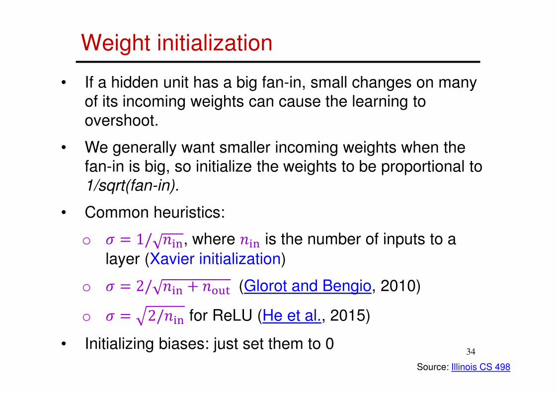
Weight initialization

• If a hidden unit has a big fan-in, small changes on many

of its incoming weights can cause the learning to

overshoot.

• We generally want smaller incoming weights when the

fan-in is big, so initialize the weights to be proportional to

1/sqrt(fan-in).

• Common heuristics:

o � 1/ �ab, where �ab is the number of inputs to a

layer (Xavier initialization)

o � 2/ �ab � �cde (Glorot and Bengio, 2010)

o � = 2/�ab for ReLU (He et al., 2015)

• Initializing biases: just set them to 0

Source: Illinois CS 498

34


• When using the ReLU nonlinearity with � = 1/ �ab it breaks.


35


• When using � = 2/�ab for ReLU (He et al., 2015)


36

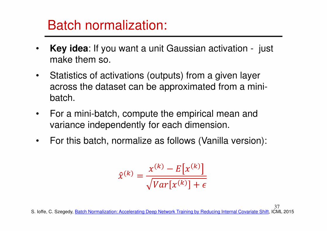
Batch normalization:

• Key idea: If you want a unit Gaussian activation - just

make them so.

• Statistics of activations (outputs) from a given layer

across the dataset can be approximated from a mini-

batch.

• For a mini-batch, compute the empirical mean and

variance independently for each dimension.

• For this batch, normalize as follows (Vanilla version):

�f(g) = �(g) − ( � g

L�\ �(g) � h

S. Ioffe, C. Szegedy, Batch Normalization: Accelerating Deep Network Training by Reducing Internal Covariate Shift, ICML 201537

Batch normalization

Usually inserted after Fully Connected

layers / (or Convolutional, as we’ll see

soon), and before nonlinearity.

Problem: do we really want a unit

Gaussian input to a tanh layer?

Solution: Allow the network to modify

the scale and bias , if needed.

FC

BN

tanh

FC

BN

tanh

...


38

Batch normalization

• Batch Normalization – full version:

�f(g) = �(g) − ( � g

L�\ �(g) � h

then allow the network to squash the range if it wants to:

� = i(g) �f(g) � j(g)where i and j are learned through the back prop.

• Note, the network can learn:

i(g) = L�\ �(g) and j(g) = ( � g

recovering the identity mapping


39

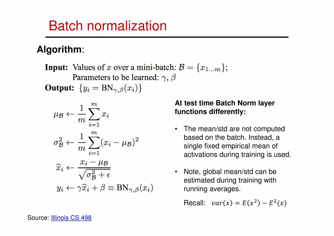
Batch normalization

Algorithm:


40

Batch normalization

Algorithm:


At test time Batch Norm layer functions differently:

• The mean/std are not computed

based on the batch. Instead, a

single fixed empirical mean of

activations during training is used.

• Note, global mean/std can be

estimated during training with

running averages.

Recall: M�\ � = ( �B − (B(�)

Batch normalization

Benefits

• Prevents exploding and vanishing gradients

• Keeps most activations away from saturation regions of

non-linearities

• Accelerates convergence of training

• Makes training more robust w.r.t. hyperparameter

choice, weight initialization

Pitfalls

• Behavior depends on composition of mini-batches, can

lead to hard-to-catch bugs if there is a mismatch

between training and test regime


42

Regularization

43

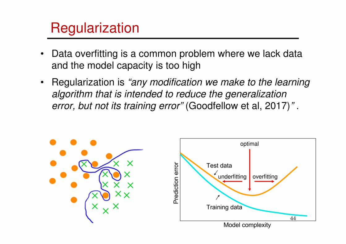
Regularization

• Data overfitting is a common problem where we lack data

and the model capacity is too high

• Regularization is “any modification we make to the learning

algorithm that is intended to reduce the generalization

error, but not its training error” (Goodfellow et al, 2017)” .

optimal

overfittingunderfitting

44

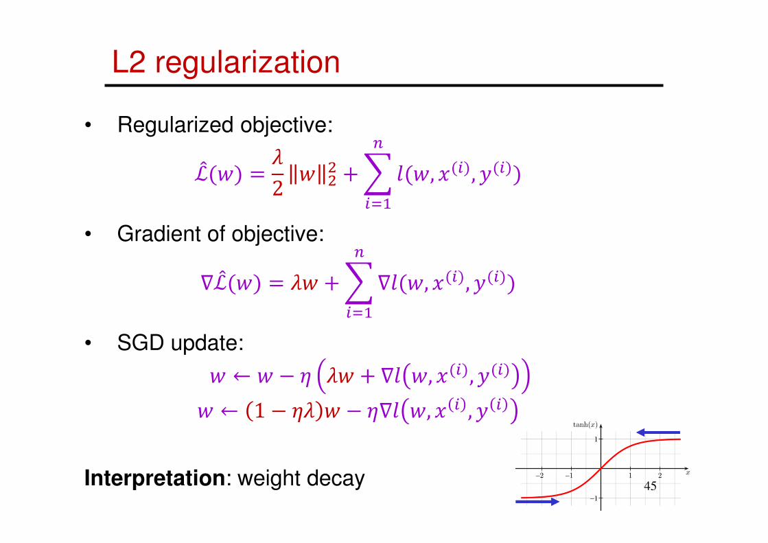
L2 regularization

• Regularized objective:

ℒk�1� l2 1 BB ��m�1, ��, ��

n

��• Gradient of objective:

∇ℒk�1� l1 ��∇m�1, ��, ��n

��• SGD update:

1 ← 1 � � l1 � ∇m 1, ��, ��1 ← 1 � �l 1 � �∇m 1, � � , � �

Interpretation: weight decay45

L1 regularization

• Regularized objective:

ℒk 1 l 1 � ��m 1, ��, ��n

�� l� 1p

p��m 1, ��, ��

n

��• Gradient: ∇ℒk 1 l sgn �1� � ∑ ∇m�1, ��, ��n��

• SGD update:1 ← 1 � �l sgn 1 � �∇m 1, ��, ��

• Interpretation: encouraging sparsity

46

Regularization: dropout

• At training time, in each forward pass, turn off some

neurons with probability 1-p

• At test time, to have deterministic behavior, use the

full network and multiply output of neuron by p

Srivastava et al. Dropout: A Simple Way to Prevent Neural Networks from Overfitting, JMLR 201447


Srivastava et al. Dropout: A Simple Way to Prevent Neural Networks from Overfitting, JMLR 201448


Intuitions:

1. Forces the network to have a redundant representation

2. prevent “co-adaptation” of units, increase robustness to

noise

3. Can be seen as a large ensemble of models that share

parameters

has an ear

has a tail

is furry

has claws

mischievous

look

X

X

X

cat

score


49

Non-redundant representation

Ensemble

Network

1

Network

2

Network

3

Network

4

Train a bunch of networks with different structures

Training

Set

Set 1 Set 2 Set 3 Set 4

Source: Lee Hung-yi50

Ensemble

y1

Network

1

Network

2

Network

3

Network

4

Testing data x

y2 y3 y4

average


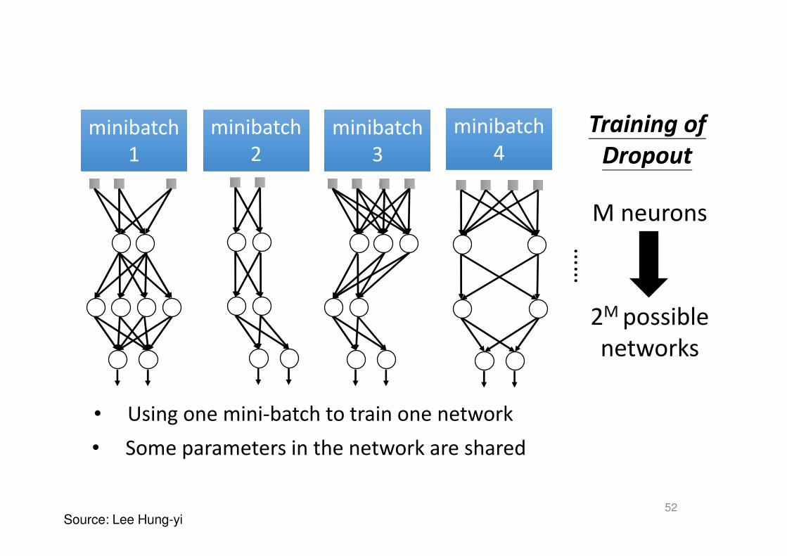
Training of

Dropout

minibatch

1

minibatch

1

……

• Using one mini-batch to train one network

• Some parameters in the network are shared

minibatch

2

minibatch

2

minibatch

3

minibatch

3

minibatch

4

minibatch

4

M neurons

2M possible

networks


testing data xTesting of Dropout

……

average

y1 y2y3

Multiply all

activations

by p

= y


Dropout Summary

54

Dropout Summary

drop in forward pass

scale at test time


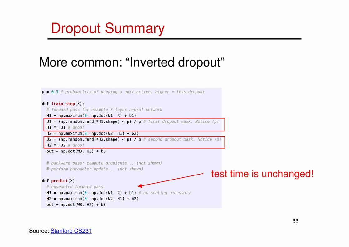
Dropout Summary

55

More common: “Inverted dropout”

test time is unchanged!


Regularization: drop connect

• Drop-Connect works similarly to dropout, except that we

disable individual weights (i.e., set them to zero), instead

of nodes.

• Drop-Connect is a generalization of Drop-out because it

produces more possible models, as there are almost

always more connections than units.

56

Regularization: Data augmentation

Intuition: If you have few examples – generate new

examples from the existing ones.

• Introduce transformations not adequately sampled in

the training data

• Geometric: flipping, rotation, shearing, multiple crops

• Photometric: Color transformations, add noise, etc.


Rorartions

57


Zooming Occlusions Cropping

Color

transformations

Add noise58


• Use many transformations. Go crazy!

• But avoid introducing obvious artifacts


59

Early stopping

• Idea: do not train a network to achieve too low training

error

• Monitor validation error to decide when to stop

60

Early stopping

• Idea: do not train a network to achieve too low training

error

• Monitor validation error to decide when to stop

61

Transfer Learning

• Transfer learning is a method where a pre-trained

network on one task is re-used on a second task

• Two possibilities:

o Use the pre-trained model as a starting point for the second-task

o Freeze the lower part of the network and retrain the last part

62

Transfer Learning

• Transfer learning is useful where we lack annotated data


63

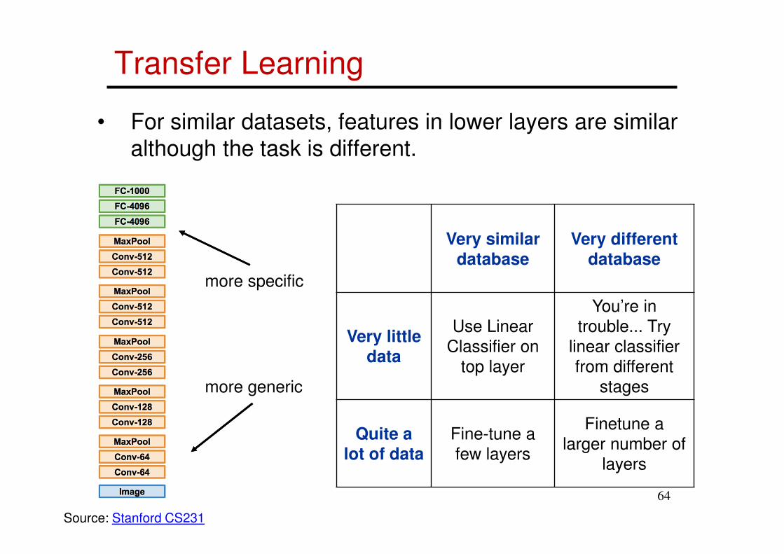
Transfer Learning

• For similar datasets, features in lower layers are similar

although the task is different.

Very similar database

Very different database

Very little data

Use Linear

Classifier on

top layer

You’re in

trouble... Try

linear classifier

from different

stages

Quite a lot of data

Fine-tune a

few layers

Finetune a

larger number of

layers

more specific

more generic


64

Regularization: Summary

• General Idea: do not train a network to achieve too low

training error and high generalization error

• Methods: Disrupt your network and constrain the

flexibility of the model

• Approaches:

- Weight decay (L2,L1)

- Dropout / drop-connect

- Early stopping

- Data augmentation

• Advanced methods:

- Transfer Learning

- add synthesized data using generative models

- add unlabeled data (semi-supervised learning) 65

Regularization: Summary

Semi-supervised:

66

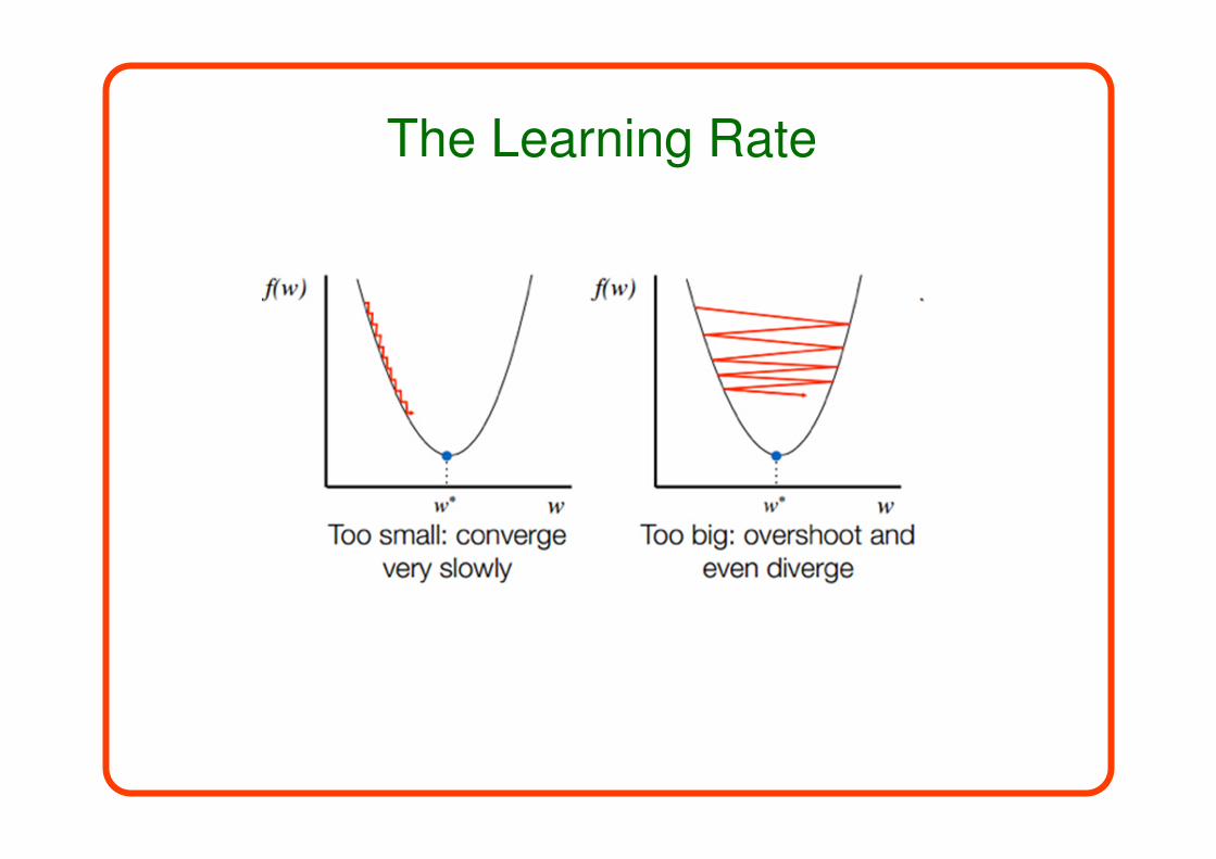
The Learning Rate

Learning Rate

How to choose the learning rate?We already studied several alternatives:

Manual tuning

Rate decay

Momentum

Adaptive learning rates (Adagrad, Adam)

Hyper-parameter Tuning

69

Supervised learning outline

1. Collect data and labels

2. Specify model: select model type, loss

function, hyperparameters

3. Train model: find the parameters of the

model that minimize the empirical loss on

the training data

• What is the right methodology for step 2?

70

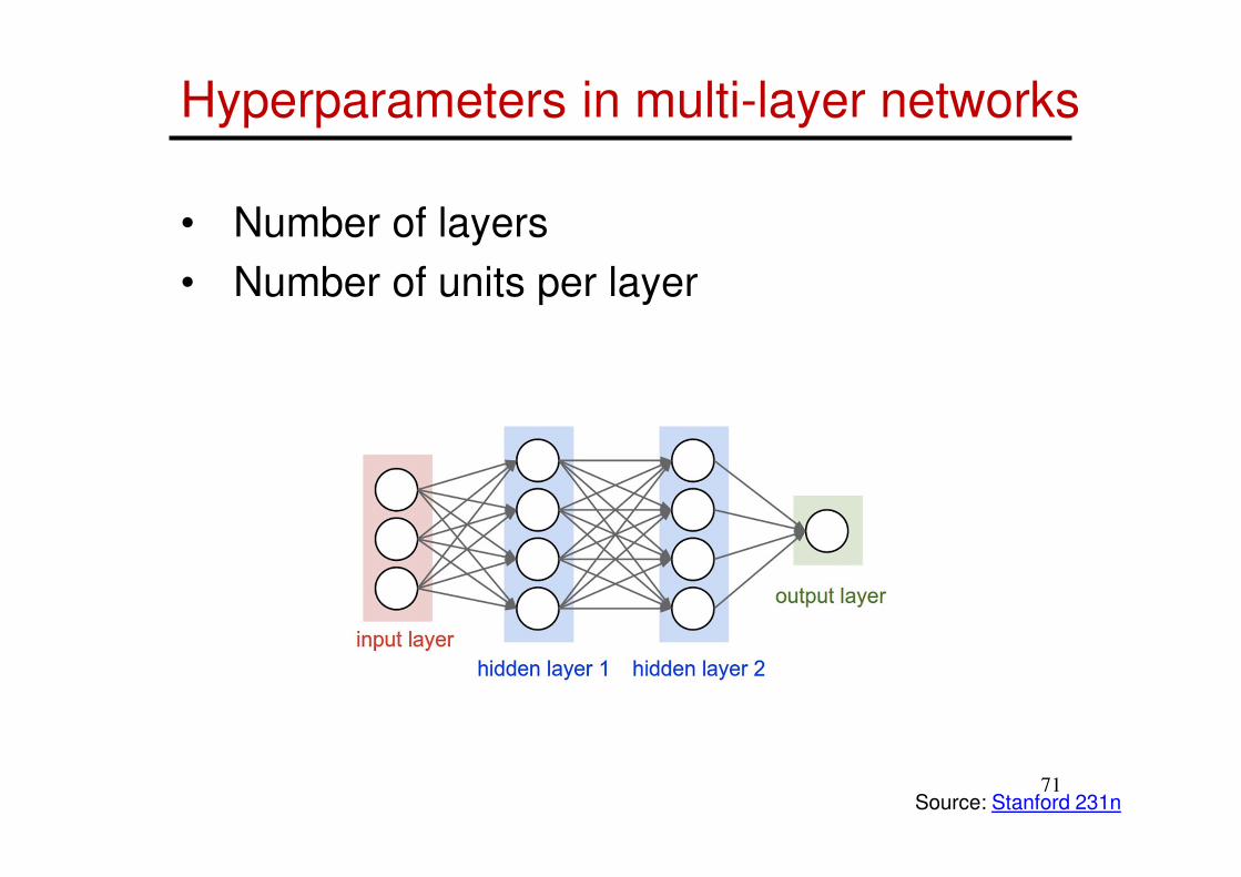
Hyperparameters in multi-layer networks

• Number of layers

• Number of units per layer

Source: Stanford 231n71


Source: Stanford 231n

Number of hidden units in a two-layer network

72







• Regularization %�, %B, l





• Regularization %�, %B, l• SGD: learning rate schedule, number of

epochs, minibatch size, dropout p, etc.

• We can think of our hyperparameter choices

as defining the “complexity” of the model and

controlling its generalization ability

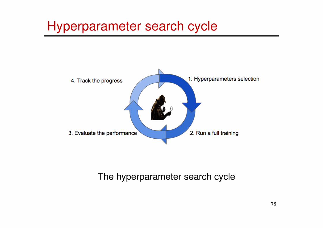
Hyperparameter search cycle

The hyperparameter search cycle

75

Hyperparameter Tuning

• Training set - used to learn the network

parameters (weights, biases)

• Validation set (Dev) – used to perform model

selection and hyper-parameters tuning

• Test set – used to assess the fully trained model

• For deep networks, Dev and Test sets should be a

small fraction of the entire set, as most of the data

is needed for training

Hyperparameter evaluation

• Another possibility of to use the k-fold cross validation

• Training is performed of k-1 folds and evaluated on the

last fold.

• This process is iterated k-times and the final evaluation is

the average of the k-results

• This technique is less common when the training process

is too long

77

Hyperparameter search

• Grid search is a traditional technique for implementing

hyperparameters. It brute forces all combinations.

• Grid search suffers from the curse of dimensionality if

data is of high dimensional space.

• Random search randomly samples the search space. It

explores more samples at each axis. Especially useful if

one axis is more important than the others.

78

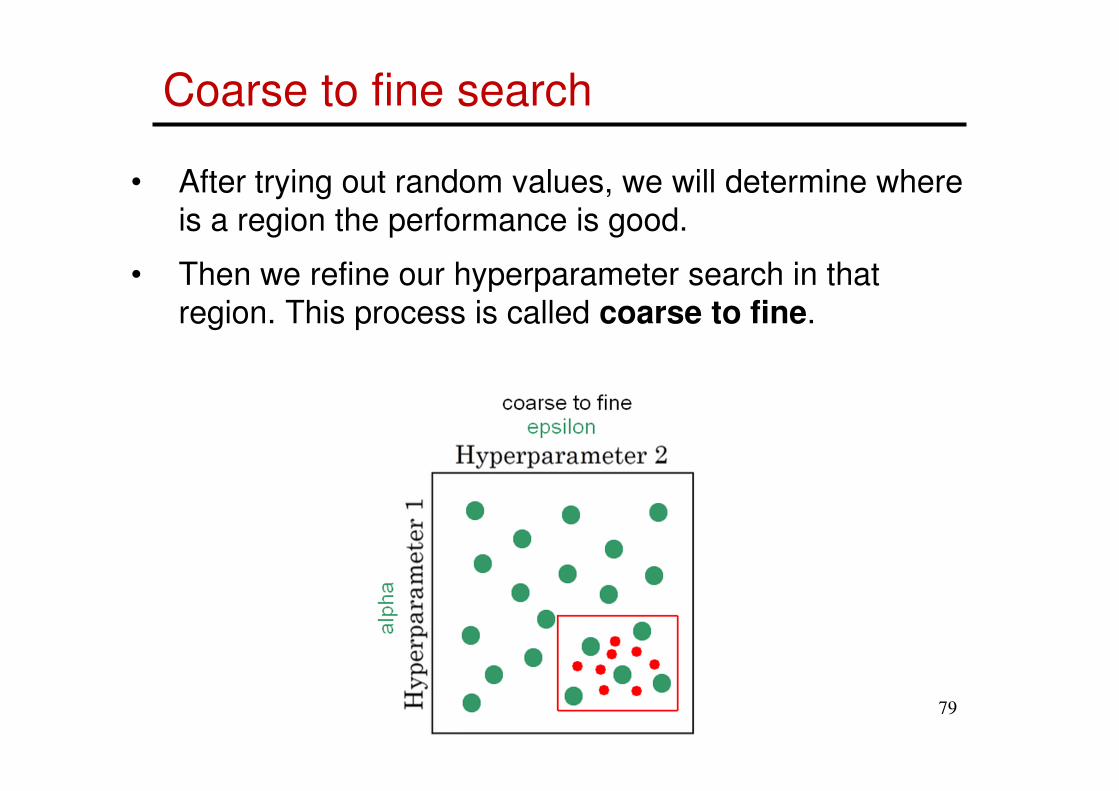
Coarse to fine search

• After trying out random values, we will determine where

is a region the performance is good.

• Then we refine our hyperparameter search in that

region. This process is called coarse to fine.

79

Log Scale Search

• Some hyper-parameters, such as, learning rate and

regularization strength, have multiplicative effects on the

training dynamics.

• Adding 0.01 to a learning rate has huge effects on the

dynamics if the learning rate is 0.001, but nearly no

effect if the learning rate when it is 10.

• For such hyperparameters search on log scale:

m��m�>�u&�� 10 ∗∗ uniform −4,0

0.0001 0.001 0.01 0.1 1.0

80

Bias vs. Variance

81

Bias vs Variance

• Supervised learning: � 4�� is unknown

• Find a model 4k that approximates 4: 4k { 4• End goal: 4k should achieve a low predictive error on

unseen data

• Underfitting: 4k is not flexible enough to approximate 4.

• Overfitting: 4k fits the training set noise

Under fitting Overfitting 82

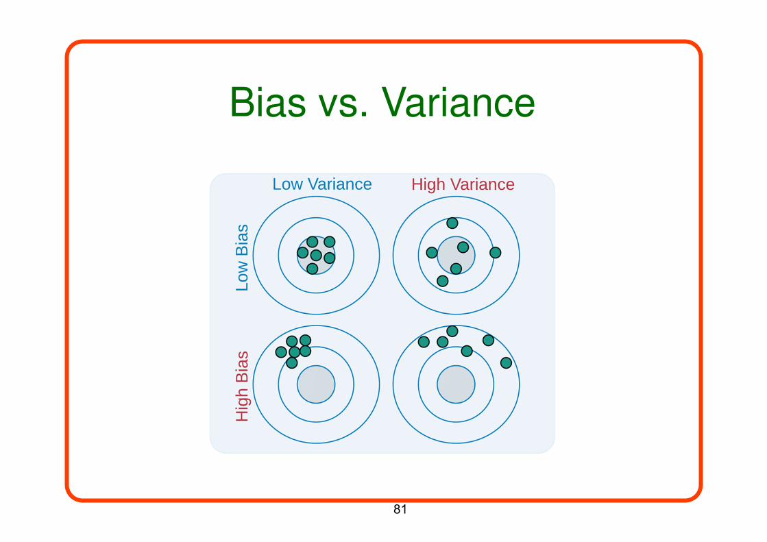
Bias vs Variance

• Bias: error due to simplifying model assumptions

• Variance: error due to randomness of training set

• The tradeoff between these components is determined

by the complexity of the model and the amount of

training data

• Generalization Error of 4k 7>�JB � M�\>��|�

High bias, low variance Low bias, high variance83

Bias vs Variance

• Bias: error term that tells you, on average, how much 4k } 4• Variance: tells you how much 4k is inconsistent over different

training sets.

underfitting

overfitting

84

Bias vs Variance

• Bias: error term that tells you, on average, how much 4k } 4• Variance: tells you how much 4k is inconsistent over different

training sets.

85

Training vs test errors

Training error

Test error

Complexity Low BiasHigh Variance

High BiasLow Variance

Err

or

Source: D. Hoiem

86

Effect of training set size

Source: D. Hoiem

Many training examples

Few training examples

Complexity Low BiasHigh Variance

High BiasLow Variance

Test E

rror

87

Effect of training set size

Source: D. Hoiem

Testing

Training

Number of training examples

Err

or

Generalization gap

Fixed model

88

The ML Recipe

Error

Train 1% 15% 15% 0.5%

Test 11% 10% 30% 1%

High

Variance

High

Bias

High

B&V

Low

B&V

89

The ML Recipe

Error

Train 1% 15% 15% 0.5%

Test 11% 10% 30% 1%

High

Variance

High

Bias

High

B&V

Low

B&V

90

• Training neural networks is still a black magic

• Process requires close “babysitting”

• For many techniques, the reasons why, when, and

whether they work are in active dispute

• Read everything but don’t trust anything

• It all comes down to (principled) trial and error

Training Summary


91

THE END

92

Training and Optimization - cs.haifa.ac.il

Documents

Transcript of Training and Optimization - cs.haifa.ac.il