Train Induced Ground Vibration – Influence of Rolling...

RIVAS

SCP0-GA-2010-265754

RIVAS_UIC_ WP5_D5_1_V02 of 53 29/09/2011

RIVAS Railway Induced Vibration Abatement Solutions

Collaborative project

Train Induced Ground Vibration – Influence of Rolling Stock State-of-the-Art Survey

Deliverable D5.1

Submission date: 30/09/2011

Project Coordinator: Bernd Asmussen International Union of Railways (UIC) [email protected]

mailto:[email protected]

RIVAS

SCP0-GA-2010-265754

RIVAS_UIC_ WP5_D5_1_V02 of 53 29/09/2011

Title Train Induced Ground Vibration – Influence of Rolling Stock State-of-the-Art Survey

Domain WP 5 Date 2011-09-23 Author/Authors Adam Mirza, Jens Nielsen, Philipp Ruest Partner BT Document Code RIVAS_UIC_ WP5_D5_1_V02 Version Status Final

Dissemination level:

Project co-funded by the European Commission within the Seventh Framework Programme

Dissemination Level PU Public X PP Restricted to other programme participants (including the Commission Services) RE Restricted to a group specified by the consortium (including the Commission) Services) CO Confidential, only for members of the consortium (including the Commission Services)

Document history

Revision Date Description

1 23/09/2011 First Draft

2 29/09/2011 Final version, reviewed by Bernd Asmussen

RIVAS

SCP0-GA-2010-265754

RIVAS_UIC_ WP5_D5_1_V02 of 53 29/09/2011

1. EXECUTIVE SUMMARY In the current report, an inventory is made of available simulation and measurement studies on the vehicle influence on ground vibration generated by rail traffic. An introduction to the theory on generation and propagation of ground vibration is followed by a few studies on the potential of optimizing vehicle design parameters in order to reduce ground vibration emissions. Finally some concluding remarks are given to the current status of the research and a possible way forward is outlined by the identification of topics interesting for future studies.

Ground vibration from railway traffic is generated either by the static axle loads moving along the track or by the dynamic forces which arises in the presence of harmonic or non-harmonic wheel and rail irregularities. The most important frequency range of ground vibration considering human exposure is approximately 5-80 Hz. The excitation by the so called quasi-static axle loads primarily leads to low frequency vibrations strongly attenuated in the direction away from the track. The frequency content of the dynamic excitation is determined by the speed of the vehicle and the wavelength contents of the irregularities exciting the wheel-rail contact patch. On a given location the vibration amplitudes will be strongly influenced by the properties of the ground and hence the vibration problem must be seen as an interaction between vehicle, track and ground.

Consideration of ground vibration in the vehicle design imposes an additional design criterion to an already over determined vehicle design. The performance related to e.g. ride comfort and gauging could come in conflict with new requirements on ground vibration and hence new design solutions must be carefully cross-checked with the compliance of already existing requirements.

Most of the research on the topic of ground vibration from railway traffic has placed its focus on the properties of the ground and the potential of different mitigation measures introduced either in the ground or on the track. Primarily three references have been found in which the vehicle design or the vehicle type has been the centre of attention. The work done within the RENVIB II project Task 6 included a parametric study on the influence of some track and vehicle parameters on the dynamic excitation of ground vibration. Based on simulations it was concluded that a reduction in wheel and rail irregularities leads to an equivalent reduction of ground vibration. The parametric study showed that a reduced un-sprung mass has a positive effect on ground vibration above 25 Hz. In fact, changing the un-sprung mass and the primary suspension stiffness causes a frequency shift in the vehicle receptance which moves the highest response to a different frequency range. The same result was seen in the parametric study performed within the CHARMEC SP18 project, which also successfully validated the simulations with measurements. Furthermore the relationship between axle load and the quasi-static excitation and the evanescent quasi-static ground response were demonstrated.

The analysis of a measurement campaign performed by SBB showed a statistical evaluation of ground vibration levels recorded from a large number of trains. Freight trains showed higher maximum vibration levels compared to regional and intercity trains. This was believed to be a consequence of one or more wheel flats being present on the freight trains. The higher axle load often associated with freight did not seem to be the primary issue. Other measurements comparing the static axle load with the vibration level in the ground also demonstrated the importance of dynamic load generated by wheel tread imperfections.

The vehicle models used in the current simulation studies were rather simple models accounting for the carbody, bogie frame and wheelset masses as well as the primary and secondary suspensions. In the RENVIB II study a quarter-car vehicle model was used, while the CHARMEC study used a model accounting for all four wheel axles of the vehicle and hence included the effects of the

RIVAS

SCP0-GA-2010-265754

RIVAS_UIC_ WP5_D5_1_V02 of 53 29/09/2011

spacing between the axle loads as well as the pitch motions of the bogie frame and the carbody. For the dynamic excitation an input spectrum of the wheel and rail irregularities was given. The track and ground models were invariant in the direction of the track and accounts for the rail, rail pad, sleeper, ballast, embankment and a ground structure consisting of a layered soil. For future simulations a similar ground model developed at KUL, Belgium, called TRAFFIC will be used. This model will be combined with a vehicle modelled in a commercial vehicle dynamic software, such as SIMPACK or GENSYS. This will allow for the use of more complex vehicle models that simplifies the cross-checking of vehicle parameters with other design targets e.g. gauging and ride comfort. For the excitation of non-harmonic wheel imperfections, such as wheel flats, the DIFF software will be used to calculate the impact load time history. A Fourier spectrum of the impact load will be calculated and used as input to the ground model.

A very rough assessment of the potential of different mitigation measures made by SBB indicates that the highest benefit-to-cost ratio is seen for measures addressed to maintenance routines and existing rolling stock. Considering the long life-cycle of railway vehicles these kinds of retrofit solutions will be crucial in order to reduce the vibration emissions from the railway within a reasonable time frame. All proposed solutions presented within the RIVAS project will be assessed both for its cost effectiveness and their respective acceptance expected from vehicle manufacturers and vehicle operators.

RIVAS

SCP0-GA-2010-265754

RIVAS_UIC_ WP5_D5_1_V02 of 53 29/09/2011

2. TABLE OF CONTENTS

1. Executive Summary .....................................................................................................................3

2. Table of contents.......................................................................................................................... 5

7

8

8

8

9

9

12

12

13

14

17

21

21

21

23

27

32

37

37

37

38

39

39

40

41

42

43

43

3. Introduction..................................................................................................................................

4. Theory ..........................................................................................................................................

4.1 Excitation...............................................................................................................................

4.1.1 Quasi-static and dynamic excitation ..............................................................................

4.1.2 Parametric excitation......................................................................................................

4.2 Propagation............................................................................................................................

5. Wheel out-of-roundness and roughness.....................................................................................

5.1 Periodic out-of-roundness ...................................................................................................

5.2 Discrete wheel defects.........................................................................................................

5.3 Maintenance criteria ............................................................................................................

6. Vehicle parameters relevant for ground vibration .....................................................................

7. Simulation and Measurement studies on rolling stock influence ..............................................

7.1 RENVIB II Phase 2. Task 6, ...............................................................................................

7.1.1 Track parameters..........................................................................................................

7.1.2 Vehicle parameters.......................................................................................................

7.2 CHARMEC SP 18...............................................................................................................

7.3 SBB measurements Prateln, Thun, Ligertz .........................................................................

8. Prediction Models ......................................................................................................................

8.1 Available prediction models and prediction results ............................................................

8.1.1 TGV – Train Ground Vibration ...................................................................................

8.1.2 TRAFFIC .....................................................................................................................

8.1.3 DIFF.............................................................................................................................

8.1.4 SIMPACK – ADAMS – GENSYS – VAMPIRE – NUCARS....................................

8.2 Vehicle modelling ...............................................................................................................

8.2.1 Vehicle models in TGV ...............................................................................................

8.2.2 Vehicle models in TRAFFIC .......................................................................................

8.2.3 Vehicle models in DIFF...............................................................................................

8.3 Track models .......................................................................................................................

RIVAS

SCP0-GA-2010-265754

RIVAS_UIC_ WP5_D5_1_V02 of 53 29/09/2011

8.3.1 TGV ............................................................................................................................. 43

44

45

46

47

47

47

47

47

48

49

50

52

8.3.2 TRAFFIC .....................................................................................................................

8.3.3 DIFF.............................................................................................................................

8.3.4 GENSYS ......................................................................................................................

8.4 Ground models ....................................................................................................................

8.4.1 TGV .............................................................................................................................

8.4.2 TRAFFIC .....................................................................................................................

8.4.3 DIFF.............................................................................................................................

8.4.4 GENSYS ......................................................................................................................

8.5 Input data.............................................................................................................................

8.5.1 Track irregularities.......................................................................................................

9. Concluding Remarks and topics for future research..................................................................

10. REFERENCES........................................................................................................................

RIVAS

SCP0-GA-2010-265754

RIVAS_UIC_ WP5_D5_1_V02 of 53 29/09/2011

3. INTRODUCTION A train running on a surface line will affect its environment by emissions of air-borne and ground-borne noise as well as ground-borne vibration. Among these emissions the perceivable ground-borne vibration have the lowest frequency content ranging from a few Hz up to around 80 Hz [1,2]. On soft grounds frequencies starting from 1 Hz may be important. The ground-borne noise consist of vibration propagating in the ground which is radiated as noise from e.g. building walls and typically hold frequencies from 30-250 Hz [1]. The highest frequency content is found in the air-borne noise radiated directly from the wheel and rail surfaces, the so called rolling noise with typical frequency range 50-5000 Hz [3]. Due to the very small variations in the air between different locations, the propagation of air-borne noise to the surroundings will be essentially equal on all sites. On the contrary, ground properties will vary significantly from one site to another and hence the propagation of ground-borne noise and vibrations will be site specific.

The excitation of noise and vibrations stem from the wheel-rail interaction and hence is primarily governed by the properties of the vehicle and the track. This is the case for excitation of air-borne and ground-borne noise with frequency content above 50 Hz [3]. Ground-borne vibrations however has an essential part of the energy concentrated to frequencies below 50 Hz. The excitation of these long-wavelength vibrations will be governed also by the ground properties and hence the excitation will also be site-specific. For these reasons the RIVAS project incorporates studies on the vehicle, the track and the ground and their interactions.

Ground vibrations induced by railway vehicles can be an issue both for low-speed freight traffic as well as high-speed passenger service. The reason for this is the many different parameters influencing the excitation, e.g. vehicle speed, axle-load and wheel and rail imperfections. Freight vehicles tend to travel at lower speeds but have in general higher axle loads and more severe wheel imperfections due to the common use of cast-iron block-braked wheels. Passenger vehicles on the other hand travel at higher speeds and hence the most effective measures to reduce excitation of ground vibrations will vary for different vehicles. The work within RIVAS WP5 aims at identifying and quantifying these parameters.

RIVAS

SCP0-GA-2010-265754

RIVAS_UIC_ WP5_D5_1_V02 of 53 29/09/2011

4. THEORY

4.1 EXCITATION

4.1.1 Quasi-static and dynamic excitation A stationary vehicle standing on a railway track imposes a set of static loads on the track concentrated to the wheel-rail contact surfaces. For a vehicle in motion these loads will be travelling along the track with the speed of the vehicle, however still being static if the wheels and the rails are free from irregularities and neglecting the influence of parametric excitation caused by the passing of sleepers. This type of excitation which consists of static loads in motion is usually referred to as quasi-static excitation and is fully determined by the axle-load and the vehicle speed. The quasi-static excitation has been studied both in theory [4,5,6] and by means of measurements [5,6,7]. From one wheel-rail contact a single wave front will be imposed by the vehicle to the ground and this will only excite propagating waves in the ground if the speed of the vehicle, and hence the speed of the wave front, reaches a natural wave speed in the ground. Below this critical speed the quasi-static excitation causes a near field response which is only significant close to the track.

In presence of wheel and rail imperfections the nominal contact forces are disturbed and a dynamic part is introduced into the excitation. In case the contact surface contains a discontinuity, e.g. a wheel flat or a rail joint the dynamic excitation will be an impulse excitation. If on the other hand the wheel and rail imperfections are of harmonic nature, such as wheel and rail roughness or track misalignment, the dynamic excitation will also be harmonic. The frequency range of the excitation will then be determined by the speed of the vehicle and the wavelengths of the imperfections. The dynamic excitation will excite all propagating modes in the ground within the frequency range of the excitation. In a situation where no propagating waves are excited by the quasi-static excitation the dynamic excitation is the only contributor to the response at a few or more metres distance from the track. Figure 4.1 illustrates the quasi-static and dynamic parts of one wheel-rail contact force.

Figure 4.1 Quasi-static and dynamic excitation in one wheel-rail contact.

RIVAS

SCP0-GA-2010-265754

RIVAS_UIC_ WP5_D5_1_V02 of 53 29/09/2011

4.1.2 Parametric excitation In figure 4.1 the rail resting on discrete sleeper supports is assumed to be infinitely stiff and any deflection of the rail in between the sleepers is neglected. In practice however a stiffness variation of the rail beam is experienced by the moving load caused by the discrete sleeper support which will introduce a second form of dynamic excitation of the wheel-rail contact surface. This is commonly referred to as parametric excitation and will have a fundamental frequency determined by the speed of the vehicle and the spacing between the sleepers. This so called sleeper passing frequency is apparent in most ground vibration measurements [6]. Commonly in Europe a sleeper spacing of about 60 cm is used which for a vehicle travelling at 100 and 200 km/h would cause a parametric excitation at about 45 and 90 Hz respectively. These frequencies are within the typical range of frequencies related to ground-borne noise and vibration. On a given track, the amplitude of the parametric excitation is varying with axle load and running speed and in turn also with frequency. The excitation increases with speed as the fundamental frequency reaches the vehicle-track resonance. Beyond this eigenfrequency the excitation declines as parts of the vehicle mass (carbody and bogie) becomes uncoupled [8].

4.2 PROPAGATION In rare cases the vibration emissions from the railway constitutes a safety risk for the railway vehicle itself. However the vibrations excited in the wheel-rail contact are primarily a problem for the environment adjacent to the railway lines. The vibration propagates in the ground and becomes problematic as it reaches buildings or other constructions in the vicinity of the track. The issues are primarily related to discomfort experienced by residents but can also be more severe and damage buildings or disturb sensitive equipment in e.g. hospitals and laboratories.

The vibration emissions reaching the far field are governed by the excitation in the wheel-rail contact, the coupling between track and embankment and the propagation properties of the ground. For a given excitation the vibration reaching the far field is highly depending on the dynamic properties of the soil and the structural composition of the soil. The stiffness, density and Poisson’s ratio determines the wave speed of the shear and longitudinal waves in the soil which sets the conditions for propagating waves in the case of a homogeneous soil without boundaries. In real life however the ground is commonly found to consist of several layers of soil with different thicknesses and varying dynamic properties, a rough illustration of this is given in figure 4.2. The layering of the ground together with the upper boundary consisting of the ground surface enables the propagation of Rayleigh waves and dispersive (frequency dependent wave velocity) modes and not only the pure shear and longitudinal waves. These wave types could carry the energy injected by the quasi-static excitation to the far field if the vehicle speed is high enough. The Rayleigh wave has the lowest wave speed among these waves and is therefore the first one to be excited which occurs for the combination of high-speed trains running on soft soils [9]. At lower speeds, or stiffer grounds, the quasi-static excitation will cause an evanescent near field which is important only close to the track.

RIVAS

SCP0-GA-2010-265754

RIVAS_UIC_ WP5_D5_1_V02 of 53 29/09/2011

Figure 4.2 Simplified illustration of a layered ground consisting of soils with varying dynamic

properties.

The dynamic excitation will have a frequency content determined by the harmonic wheel and rail imperfections and the speed of the vehicle. This will excite the modes in the ground which are in the frequency range of the excitation. Observations of a rise in vibration amplitude in the ground around 10-20 Hz have been made [10], which theoretical studies have shown to be caused by an onset of modes in the upper layer of the soil [11].

The dispersive nature of the modes in the ground means that the quasi-static axle load will excite given modes at different frequencies depending on the vehicle speed (given that the lowest wave speed in the ground is exceeded). Furthermore the dynamic excitation from harmonic wheel and rail imperfections will excite modes with different wave speeds depending on the frequency of the excitation. In order to better understand and visualize the excitation of dispersive modes, a so called dispersion diagram is used. It plots the relation between frequency, f and wave number k=ω/c of a dispersive wave, where ω is the angular frequency and c the phase velocity of the wave, see figure 4.3. Non-dispersive waves have a constant ratio between frequency and wave number and hence are seen as straight lines in the plot. Dispersive modes on the other hand have a slope which varies with frequency. The excitation from a quasi-static axle-load travelling at constant speed v is represented by a straight line, with a slope equal to 2π/v, originating from (0,0) in the dispersion diagram. Figure 4.4 shows the same kind of dispersion diagram but including the dynamic excitation from a harmonic load with f=40 Hz travelling at different speeds. The dynamic excitation from a stationary, single harmonic load exciting the ground is seen as a straight vertical line originating from (f,0). Due to the Doppler effect a harmonic load travelling at constant speed will be represented by two lines; one with positive slope equal to 2π/v and one with negative slope equal to -2π/v. Both lines are originating from (f,0). For more details see [3]. The intersection of a load line with a line representing a wave or a dispersive mode may lead to large displacement amplitudes in the ground.

RIVAS

SCP0-GA-2010-265754

RIVAS_UIC_ WP5_D5_1_V02 of 53 29/09/2011

Figure 4.3. Dispersion diagram of a ground model consisting of one layer on top of a half-space including load lines from quasi-static loads travelling at 100, 150, 200 and 250 km/h. Calculation

performed with script developed at ISVR, UK. load 100 km/h, load 150 km/h, • • • load 200 km/h, • load 250 km/h,

Rayleigh wave layer 1, • • • Shear wave layer 1, • Pressure wave layer 1,

Dispersive modes

Figure 4.4 Dispersion diagram of a ground model consisting of one layer on top of a half-space including load lines from a harmonic excitation with f=40 Hz travelling at 83, 112 and 150 m/s [10].

RIVAS

SCP0-GA-2010-265754

RIVAS_UIC_ WP5_D5_1_V02 of 53 29/09/2011

5. WHEEL OUT-OF-ROUNDNESS AND ROUGHNESS The importance of wheel and rail imperfections is evident when considering the dynamic excitation of ground-borne vibration. Limiting the focus to the rolling stock, wheel out-of-roundness (OOR) and roughness should be considered as significant causes but also subjects of possible improvements. Wheel-rail contact forces excited by wheel imperfections are problematic for several reasons as they give rise to noise, vibrations and cause wear and damage to both vehicle and track. The problem at hand is determined by the type of imperfection present on the wheel, e.g. wheel flat, roughness, eccentricity or polygonization together with the speed of the vehicle. Periodic out-of-roundness with one or more wavelengths around the wheel circumference gives rise to a harmonic excitation while a wheel flat leads to an impulse excitation. The resulting vibration level in the ground will be dependent on the track- and ground receptances which varies from one site to another. Addressing the wheel imperfections will however lead to a general reduction of vibration on the entire network (excluding problematic locations where rail irregularities are dominating or poor soil conditions constitute the fundamental problem).

5.1 PERIODIC OUT-OF-ROUNDNESS An overview of causes, consequences and treatments of periodic out-of-roundness is given in [12]. Periodic OOR with wavelengths ranging from approximately 14 cm up to one wheel circumference is found primarily on disc-braked wheels while block-braked wheels hold more corrugation with smaller wavelengths in the range 3-6 cm. The latter is found to be a consequence of the heat generation during breaking which causes local material expansion of the tread and in turn uneven wear [13]. Furthermore almost all wheels suffer to some extent from eccentricity which is a consequence of misalignment during profiling or re-profiling. Considering the speed of different vehicle types and the most important frequency range of ground vibration it is clear that the long wavelength OOR is the primary issue. Corrugation and roughness primarily excites rolling noise which to this day has been given considerably much more attention compared to ground vibrations.

The longest wavelength of a periodic wheel OOR is equal to one wheel circumference. This, together with the speed of the vehicle sets the lower frequency limit of the excitation. Lower frequencies in the spectrum must then be associated with track irregularities or quasi-static excitation. Table 5.1 gives the wavelength range of the excitation from OOR for vehicles running at different speeds. The excited frequencies are assumed to be in the 5-80 Hz range which is pointed out to be the most important one considering human exposure.

RIVAS

SCP0-GA-2010-265754

RIVAS_UIC_ WP5_D5_1_V02 of 53 29/09/2011

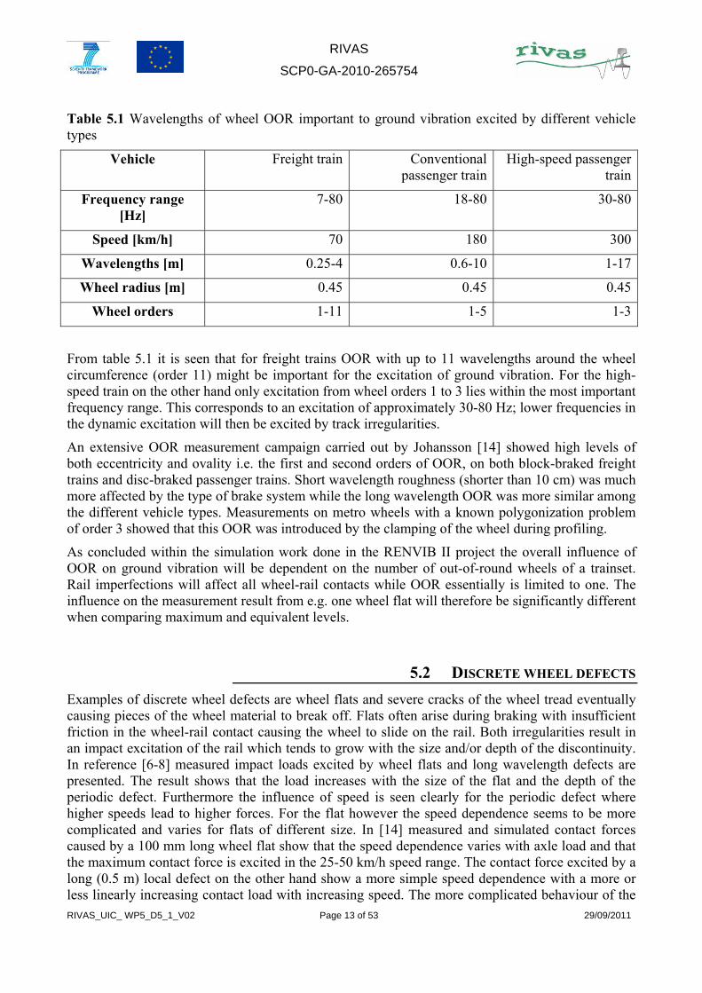
Table 5.1 Wavelengths of wheel OOR important to ground vibration excited by different vehicle types

Vehicle Freight train Conventional passenger train

High-speed passenger train

Frequency range [Hz]

7-80 18-80 30-80

Speed [km/h] 70 180 300

Wavelengths [m] 0.25-4 0.6-10 1-17

Wheel radius [m] 0.45 0.45 0.45

Wheel orders 1-11 1-5 1-3

From table 5.1 it is seen that for freight trains OOR with up to 11 wavelengths around the wheel circumference (order 11) might be important for the excitation of ground vibration. For the high-speed train on the other hand only excitation from wheel orders 1 to 3 lies within the most important frequency range. This corresponds to an excitation of approximately 30-80 Hz; lower frequencies in the dynamic excitation will then be excited by track irregularities.

An extensive OOR measurement campaign carried out by Johansson [14] showed high levels of both eccentricity and ovality i.e. the first and second orders of OOR, on both block-braked freight trains and disc-braked passenger trains. Short wavelength roughness (shorter than 10 cm) was much more affected by the type of brake system while the long wavelength OOR was more similar among the different vehicle types. Measurements on metro wheels with a known polygonization problem of order 3 showed that this OOR was introduced by the clamping of the wheel during profiling.

As concluded within the simulation work done in the RENVIB II project the overall influence of OOR on ground vibration will be dependent on the number of out-of-round wheels of a trainset. Rail imperfections will affect all wheel-rail contacts while OOR essentially is limited to one. The influence on the measurement result from e.g. one wheel flat will therefore be significantly different when comparing maximum and equivalent levels.

5.2 DISCRETE WHEEL DEFECTS Examples of discrete wheel defects are wheel flats and severe cracks of the wheel tread eventually causing pieces of the wheel material to break off. Flats often arise during braking with insufficient friction in the wheel-rail contact causing the wheel to slide on the rail. Both irregularities result in an impact excitation of the rail which tends to grow with the size and/or depth of the discontinuity. In reference [6-8] measured impact loads excited by wheel flats and long wavelength defects are presented. The result shows that the load increases with the size of the flat and the depth of the periodic defect. Furthermore the influence of speed is seen clearly for the periodic defect where higher speeds lead to higher forces. For the flat however the speed dependence seems to be more complicated and varies for flats of different size. In [14] measured and simulated contact forces caused by a 100 mm long wheel flat show that the speed dependence varies with axle load and that the maximum contact force is excited in the 25-50 km/h speed range. The contact force excited by a long (0.5 m) local defect on the other hand show a more simple speed dependence with a more or less linearly increasing contact load with increasing speed. The more complicated behaviour of the

RIVAS

SCP0-GA-2010-265754

RIVAS_UIC_ WP5_D5_1_V02 of 53 29/09/2011

contact force exited by a wheel flat is caused by the potential loss of contact between wheel and rail which is governed by the size and depth of the flat, the speed and the axle load [15,16].

Previous studies on wheel-rail contact forces and the influence of wheel and rail defects primarily have focused on damage and noise. The excitation of a wheel flat has been investigated in terms of peak contact forces in order to determine the risk of wheel or rail rupture. When estimating the influence on ground vibration, the frequency content of the excitation needs to be known and compared with the track and ground response. Figure 5.1 shows calculated contact force spectra excited by a wheel flat on Regina and X2 vehicles [17]. The wide frequency range included for rolling noise leaves a poor frequency resolution in the range important for ground vibration. It is however clear that the maximum force level is excited at a low frequency which is concluded to belong to the so called P2 resonance at approximately 80 Hz. This resonance occurs when the un-sprung mass, rail and sleepers move in phase on the sleeper support stiffness.

Figure 5.1 Calculated Fourier spectrum of wheel-rail contact force for leading wheel-set. Excitation

by a wheel flat of length 0.06 m and depth 0.45 mm. Vehicle speed 200 km/h. Solid: Regina non-rotating, dashed: Regina rotating, dotted: X2 [17]

5.3 MAINTENANCE CRITERIA The removal of wheel tread defects and the restoration of the original tread profile are done primarily in order to reduce the wheel-rail contact forces to prevent further wheel and rail damage and to ensure ride safety. The reduction of noise and vibration are secondary benefits from a smooth and regular wheel tread but the maintenance criteria are more commonly related to the magnitude of the contact force between wheel and rail.

Table 5.2 is taken from the EN standard 15313 - Railway application – In-service wheelsets operation requirements – In-service and off-vehicle wheelset maintenance (Table 7) [18]. It shows the maximum permissible length of wheel tread defects such as flats, metal build up, material loss etc. for different axle load, wheel diameter and speed intervals. In general a high speed and high axle load in combination with a small wheel diameter is anticipated to cause higher wheel-rail

RIVAS

SCP0-GA-2010-265754

RIVAS_UIC_ WP5_D5_1_V02 of 53 29/09/2011

contact forces and contact stresses in the presence of tread defects and hence is associated with a stricter requirement on the limit length of the defect.

Table 5.2 Limit length of wheel tread defects depending on axle load, speed and wheel diameter according to Table 7 of EN 15313.

The same EN standard includes permissible levels of circularity defects, i.e. the maximum allowable deviations from the nominal wheel radius. Table 5.3 shows the limiting values for different wheel diameters and speeds.

Table 5.3 Maximum permissible circularity defects according to Table I.1 of EN 15131.

Table 5.4 shows the alarm limits of the vertical wheel-rail contact force Q in different countries taken from reference [19]. In Germany and South Africa a requirement is put on the dynamic load factor which is calculated from the mean load Qmean=mean(Q) and the maximum dynamic load increment Qdyn=max(Q)-mean(Q). These are low-level alarm values which are used to indicate wagons which should be taken out of traffic at the time for the next scheduled maintenance.

RIVAS

SCP0-GA-2010-265754

RIVAS_UIC_ WP5_D5_1_V02 of 53 29/09/2011

Table 5.4 Alarm limits for wheel-rail contact forces in different countries taken from [19].

The requirements on tread defects and contact forces are set to prevent wheel and rail damage and guarantee safe rail traffic. Its relevance for ground vibration is however unknown and a further investigation on this could be considered a first step in defining new requirements on tread defects in order to limit vibration excitation.

RIVAS

SCP0-GA-2010-265754

RIVAS_UIC_ WP5_D5_1_V02 of 53 29/09/2011

6. VEHICLE PARAMETERS RELEVANT FOR GROUND VIBRATION

Railway induced ground vibration – as discussed in other chapters – depends on a variety of factors influencing dynamic and quasi-static excitation as well as propagation through the track system.

The key factors of the vehicle / track system which determine ground vibration are related to the track design and the maintenance of wheel and rail:

• Design of the track, more precisely the properties of the track mass/spring/damping system consisting of rail, pads, sleeper, ballast, slab, embankment

• Impact excitation from track discontinuities like switches & crossings and insulation joints

• Wheel / rail surface quality, roughness incl. corrugation, out-of-roundness, dents, flats

The potential for controlling ground vibration by a variation of the railway vehicle design is in reality limited. The concept and parameters of a vehicle and its bogie or running gear are typically over-determined by other requirements like vehicle dynamics, durability, reliability, weight and cost. A reduction of the induced ground vibration, respectively a shift of its frequency, can in principle be achieved by the following vehicle design approaches:

• Resilient wheels, which are hardly accepted by any customer except for LRV. Resilient wheels are incompatible with wheel-mounted brake discs (due to geometry) and with tread brakes (due to thermal impact). As a consequence resilient wheels necessitate axle mounted brake discs for which a motor bogie does often not offer sufficient space – unless the mechanical braking is permitted to be reduced and substituted by electric braking or the brake discs are mounted differently (as described under ‘unsprung mass’).

Resilient wheels lead to higher levels of rolling noise, more precisely a higher wheel contribution, due to the reduced stiffness between rim and web which outweighs the damping introduced by the rubber and results in higher vibration amplitudes of the rim.

• Lower unsprung mass, which can only be achieved through a change of the bogie concept as described below – since the weight of unsprung elements is anyway reduced within the limits of structural integrity for affordable and accepted production methods and materials. The unsprung mass of most railway vehicles consists of the wheelset and axle bearings with a part of the axle guides, the wheel or axle mounted brake discs (if applicable) and the part of the drive mounted on the axle.

A key concept with minimized unsprung mass suitable for most motor bogies is a fully suspended drive, instead of a partly or semi suspended drive, typically with a hollow shaft driving the wheelset.

Unsprung brake disc(s) on the wheels or axle could basically also be reduced or eliminated although their proportion of the unsprung mass is normally limited. While composite/carbon ceramic brake discs would be too expensive, a simple reduction of the number or size of brake discs could be realistic for electric motor bogies provided that the mechanical braking is permitted to be partly substituted by more electrical braking. A different arrangement with brake disc(s) not mounted on wheels or axles, but e.g. between the two gear stages, can also be considered. In case of a fully suspended drive with hollow shaft the brake disc(s) could

RIVAS

SCP0-GA-2010-265754

RIVAS_UIC_ WP5_D5_1_V02 of 53 29/09/2011

also be mounted on the hollow shaft, i.e. partly suspended, but for most vehicles/bogies except locomotives the required space is not available respectively the suspension displacement too high.

A more radical concept with lower unsprung mass could be a bogie or running gear with independent wheels instead of wheelsets, which requires radial steering (in order to control vehicle dynamics).

• Softer primary suspension, which causes higher spring deflection and roll angle, jeopardizing the gauging. This issue could be offset by a secondary anti-roll bar with inclined rods which affects the ride comfort or by the addition of a primary anti-roll bar which obviously increases complexity and cost. Basically the suspension stiffnesses of a railway vehicle are over-determined by the conflicting requirements related to derailment, gauging, deflection and comfort so that there’s hardly any room for ground vibration to be considered.

• Change of wheelbase, which (based on an optimized bogie design) means a longer wheelbase, so adding weight.

• Avoidance of cast iron tread brakes, a guideline which is anyway followed for rolling noise concerns related to roughness growth – unless tread braking with cast iron blocks is specifically required by the customer e.g. for shunting.

The vehicle parameters which mainly influence the ground vibration can differ substantially for the various vehicle / bogie designs and classes. In the following table ‘High value’ and ‘Low value’ correspond to the parameters of section 7.2 while ‘Upper limit’ and ‘Lower limit’ are intended to show the full range of common design parameters (in normal operation condition) for metros, electric / diesel multiple units, coaches and high speed trains. Differing parameters of locomotives and freight wagons with Y25 bogies are listed in the respective columns:

Table 6.1 Typical range of vehicle parameters relevant for ground vibration.

Parameter High value, EMU

Low value, EMU

Upper limit Lower

limit

Loco, upper Freight

wagon

Carbody mass, mc [kg] 4.5×104 3.5×104 Bogie frame mass, mb [kg] 6.0×103 4.0×103 6.0×103 2.0×103 7.5×103 2.1×103

Wheelset mass, mw [kg] 2.0×103 1.6×103 2.8×103 1.2×103 4.5×103 1.4×103 Half distance between bogie centres, lb [m] 12.0 7.0 6.0 Half distance between axles, lw [m] 1.45 1.25 1.0 0.9 Primary suspension vertical dynamic stiffness per axle, k1 [N/m] 2.8×106 2.0×106 5.0×106 1.8×106 8.0×106 2.6×106

Primary suspension vertical viscous damping per axle, c1 [Ns/m] 4.0×104 2.0×104 8.0×104 1.0×104

Secondary suspension vertical dynamic stiffness per bogie, k2 [N/m] 8.0×105 4.0×105

Secondary suspension vertical damping per bogie, c2 [Ns/m] 3.0×104 1.0×104 6.0×104 0.5×104

Axle load [kg] 21.0×103 8.0×103 22.0×103 Radial stiffness of resilient wheel [N/m] rigid 2.0×108

RIVAS

SCP0-GA-2010-265754

RIVAS_UIC_ WP5_D5_1_V02 of 53 29/09/2011

It can be analyzed in more detail which design changes, e.g. resilient wheel or reduction of unsprung mass, could possibly be realized for which vehicle and bogie type and how the associated change of parameters is expected to influence the ground vibration.

Modification of a large number of existing vehicles can be very expensive. Furthermore the modifications of new rolling stock might drive both cost and could face strong resistance from those who fear the change of an already validated design. No complete assessment of the cost related to benefit of different measures addressed to the vehicle has been found. However figure 6.1 and table 6.2 show an indicative separation of different measures with respect to their respective likelihood of being implemented and their benefit-to-cost ratio. This starting point is taken from an initial study on mitigation measures for rolling stock performed by SBB [20].

Figure 6.1 Indicative separation of rolling stock measures for reduced ground vibration with respect

to likelihood of implementation and benefit-to-cost ratio [20].

RIVAS

SCP0-GA-2010-265754

RIVAS_UIC_ WP5_D5_1_V02 of 53 29/09/2011

Table 6.2 List of rolling stock measures for reduced ground vibration numbered in figure 6.1 [20]

Measures applicable on the vehicle Maintenance and prevention of wheel

imperfections 9 Improving the brakes on Re420,

Re450 and Re620.

1 Detection of OOR and improved wheel maintenance

10 Optimal adjustment of brake parameters

2 Improved operation of rolling stock: cargo hand break, breaking activity, fluent operation

11 Wheel material quality

3 Improved time plan and minimum on uneven track

12 Anti-vibration resonators

4 Improved record of vehicle status for optimized maintenance

New rolling stock

5 Prevention of wheel flats by detection of hot boxes

13 Reduction of un-sprung mass of locomotives

6 Adjust track pricing (according to wheel condition)

14 Brake quality optimization

7 Installation of under-floor re-profiling machines (at least 40 min/wheelset)

15 Radial steering of locomotives

Existing rolling stock 16 Axle spacing

8 Replace cast iron blocks with K-blocks on freight wagons

17 Resilient wheels

It can be seen in table 6.2 that the measures most probable to be realized are those related to an improved maintenance, optimal adjustment of existing systems e.g. brakes, or design changes on new rolling stock. Furthermore the measures which are estimated to have the highest benefit-to-cost ratio are those related to maintenance and improvements on existing rolling stock.

RIVAS

SCP0-GA-2010-265754

RIVAS_UIC_ WP5_D5_1_V02 of 53 29/09/2011

7. SIMULATION AND MEASUREMENT STUDIES ON ROLLING STOCK INFLUENCE

7.1 RENVIB II PHASE 2. TASK 6, If nothing else is stated, pictures, results and conclusions in the following section are taken from reference [21].

AEA Technology Rail performed a study based on numerical simulations of ground vibration within the RENVIB II project. The study included a parametric study of the influence of vehicle and track parameters and wheel and rail roughness on the ground vibration. The track parameters included mass and stiffness properties of the rail, rail pads, sleepers and ballast. The vehicle influence was investigated through the effect of un-sprung mass, suspension type (one stage or two stage suspension).

For the predictions the AEA Technology Rail CIVET model was used which only considers the dynamic excitation from roughness. The track is modelled with a rail beam resting on rail pads and sleepers which are modelled with distributed stiffness and mass creating a continuous support of the rail. The ground is modelled with a three dimensional half-space. A quarter car vehicle model is used consisting of ¼ of the carbody mass, ½ of the bogie mass and one wheelset mass which is un-sprung from the track. The ground vibration from dynamic excitation at a receiver point on the surface of the half-space is calculated for a given roughness input. The roughness input describes the vertical track irregularities and can also be used to include wheel roughness and out-of-roundness by use of the combined effective roughness of wheel and rail. A separate calculation tool is used to predict the periodic deflection of the rail beam caused by discrete sleeper support. The deflection is then included in the CIVET model with the roughness input.

7.1.1 Track parameters The parametric study of track parameters shows a 5-20 dB reduction in the 80-250 Hz frequency range. The largest improvement is seen from softening the rail pad and the ballast layer however this tend to worsen the situation below 60 Hz due to a shift of resonances towards lower frequencies. This shift is considered not to be beneficial for ground vibration. One example of the results obtained in the study is given in figure 7.1. Here also the combined effect of altering rail pad and ballast stiffness is presented. The report does not comment on the speed or the roughness used in these calculations. Considering that the CIVET model only accounts for dynamic excitation some kind of roughness input must have been included. Most probably a uniform broadband spectrum of roughness has been used in order to excite all the natural frequencies of the train-track system. With this kind of excitation the speed information will be less important in a study based on comparing thevibration level difference between two track designs

RIVAS

SCP0-GA-2010-265754

RIVAS_UIC_ WP5_D5_1_V02 of 53 29/09/2011

Figure 7.1 Predicted improvements presented as vibration level differences between a baseline

track and tracks with different combinations of rail pad and ballast stiffness.

When searching for relevant rail roughness input data, differences of up to 40 dB in some wavelength ranges were found in available measurement data. For the simulations two cases of combined rail and wheel roughness were created; one with rough, corrugated however continuously welded rail and another with relatively smooth rail. Both cases account for the roughness of a relatively smooth disc-braked wheel and the deflection of the rail beam in between the sleepers calculated separately. In total the two cases differed about 15 dB in roughness level with some exceptions in the spectrum. Figure 7.2 shows the roughness input for the “rough” and the “smooth” cases and also the baseline roughness used for comparison. In figure 7.3 the result from the calculations using the CIVET model and the two levels of roughness can be seen for a vehicle speed of 80 km/h.

Figure 7.2 Input of combined roughness used for the CIVET model.

RIVAS

SCP0-GA-2010-265754

RIVAS_UIC_ WP5_D5_1_V02 of 53 29/09/2011

Figure 7.3 Predicted ground vibration level for the “rough” and the “smooth” cases presented as

vibration level differences compared to the baseline roughness denoted “control”. Train speed: 80 km/h.

The result in figure 7.3 shows that the difference in roughness level between the two tracks more or less translates into a difference in ground vibration level which is expected from a linear model. It is concluded that a higher vehicle speed generally leads to higher vibrations levels although a reduction might be seen at specific frequencies where the roughness excitation moves out of phase with the track response.

From the large spread found in rail roughness level among different sites it is concluded that a better maintenance of the track would be the most effective measure to reduce ground vibration. In order to achieve this, the value of a better and more accurate measurement procedure for vertical track irregularities in the relevant wavelength range is underlined. Considering that ground vibration is excited by the combined roughness of wheel and rail these kinds of measurements ought to include also wheel roughness and out-of-roundness.

7.1.2 Vehicle parameters Except from vehicle speed, the un-sprung mass, suspension design, axle load and the wheel condition are pointed out to be the key factors in predicting the influence of the vehicle on ground vibration. For the following simulations the un-sprung mass, suspension design and the wheel condition are chosen while concluding that a proper simulation of the influence of axle load would require the quasi-static excitation to be included.

The vehicle design was first investigated through simulations including the un-sprung mass and the suspension design of a vehicle running at 80 km/h. The different configurations are summarized in table 7.1. The wheel roughness was set to that of the “control” case in figure 7.2. The result is presented in figure 7.4.

RIVAS

SCP0-GA-2010-265754

RIVAS_UIC_ WP5_D5_1_V02 of 53 29/09/2011

Table 7.1 Configurations of un-sprung mass and suspension properties used in the simulations

Figure 7.4 Predicted improvements presented as vibration level differences between the baseline vehicle and vehicles with modified un-sprung mass and suspension properties according to Table

7.1

The effect of the un-sprung mass is seen above 25 Hz with a clear improvement by reduced mass. The effect of the suspension properties is not quite as clear since the different configurations

RIVAS

SCP0-GA-2010-265754

RIVAS_UIC_ WP5_D5_1_V02 of 53 29/09/2011

contain changes to both un-sprung mass and the stiffness and damping of the primary suspension. The combination of un-sprung mass and suspension stiffness is expected to determine the vehicle resonance frequency and hence a change in these parameters is shifting the resonance.

The effect of wheel roughness has been investigated in the same way as for the rail roughness. Two cases of combined roughness including a “rough” and a “smooth” wheel was created with data from a tread-braked wheel and a disc-braked wheel respectively. The two cases are given in figure 7.5 where the separate wheel roughness also is presented. The longest wavelengths are unaffected by the wheel roughness due to the limited wheel circumference.

Figure 7.5 Two cases of combined roughness with a rough tread-braked wheel and a smooth disc-

braked wheel.

The result of the simulations with a vehicle speed of 80 km/h is given in figure 7.6 as the delta between the “rough” and the “smooth” case. Furthermore the results of having a high roughness on half of the wheels or on 1 out of 16 wheels are presented. The reduction from having a high roughness on half of the wheels only is about 3 dB in the whole spectrum except for where resonances could be expected to influence the result. This result implies that the current way of analyzing the ground vibration is rather insensitive to having a high roughness on only a few of the wheels or having a single wheel flat on an entire trainset. It is pointed out in the report that the differences seen from these simulations would be significantly reduced in the case of a higher rail roughness.

RIVAS

SCP0-GA-2010-265754

RIVAS_UIC_ WP5_D5_1_V02 of 53 29/09/2011

Figure 7.6 The result of varying wheel roughness on the ground vibration presented as a delta

between the two cases given in figure 7.5.

Following is a discussion on the effects of including the quasi-static excitation. Among the vehicle parameters included in the study only the un-sprung mass will have an effect on the quasi-static excitation through its effect on the total axle load. Furthermore the quasi-static component will only be significant in the near field of the track and hence for vibration problems at further distance mitigation measures acting on the quasi-static excitation will be ineffective.

RIVAS

SCP0-GA-2010-265754

RIVAS_UIC_ WP5_D5_1_V02 of 53 29/09/2011

7.2 CHARMEC SP 18 If nothing else is stated, pictures, results and conclusions in the following section are taken from reference [22].

Within the project SP18 performed at Chalmers Railway Mechanics (CHARMEC) the influence of the vehicle on ground-borne vibration was studied through both simulations and measurements. For the simulations the Train Ground Vibration (TGV) model developed at the Institute of Sound and Vibration at the University of Southampton was used in a parametric study of nine different vehicle parameters. The parameters included the masses of the vehicle (carbody, bogie frame and un-sprung mass), a two-stage suspension (stiffness and damping of the primary and secondary suspension) and the geometric properties of the vehicle including the axle spacing and the distance between bogies.

The TGV model included a model of the vehicle, the track and the ground and it accounted for both quasi-static and dynamic excitation. The track model used was that of a ballasted track with UIC 60 rail resting on rail pads and discrete sleeper support on top of an embankment. The ground was modelled with several elastic layers of different depth representing layers of soil with different dynamic properties e.g. stiffness, damping and density. The vehicle and ground models are shown in figure 7.7.

Figure 7.7 Left: vehicle model including masses and the stiffness and damping properties of a two stage suspension, right: ground model consisting of several elastic layers of soil.

The parametric study was performed with a track and ground model corresponding to a test site in Sweden which was used for experimental validation of the simulations. The ground model data is given in table 7.2. As a baseline, a model of a two car Bombardier Regina EMU was used which was modified with upper and lower values of the nine vehicle parameters. These values are given in table 7.3.

RIVAS

SCP0-GA-2010-265754

RIVAS_UIC_ WP5_D5_1_V02 of 53 29/09/2011

Table 7.2 Ground model parameters

Model (site) Layer

Young’s modulus,

E [MPa]

Poisson’s ratio, υ

Density, ρ

[kg/m3]

Loss factor, η

Thickness, h

[m]

1 50 0.300 1800 0.2 2.0 2 70 0.300 1800 0.2 2.0

Gre

by

Half-space 500 0.300 2000 0.2 inf

Table 7.3 Upper and lower values of the vehicle model. The baseline value is the arithmetic average of the upper and lower value.

Parameter Coded variable

High value

Low value

Carbody mass, mc [kg] X1 4.5×104 3.5×104 Bogie frame mass, mb [kg] X2 6.0×103 4.0×103 Wheelset mass, mw [kg] X3 2.0×103 1.6×103 Half distance between bogie centres, lb [m] X4 12.0 7.0 Half distance between axles, lw [m] X5 1.45 1.25 Primary suspension vertical dynamic stiffness per axle, k1 [N/m] X6 2.8×106 2.0×106

Primary suspension vertical viscous damping per axle, c1 [Ns/m] X7 4.0×104 2.0×104

Secondary suspension vertical dynamic stiffness per bogie, k2 [N/m] X8 8.0×105 4.0×105

Secondary suspension vertical damping per bogie, c2 [Ns/m] X9 3.0×104 1.0×104

In order to conduct a full parametric study with the nine vehicle parameters a total of 29 = 512 different simulation would have been required. To avoid computational work a fractional factorial design (FFD) of resolution IV was chosen. This enables to resolve the effects of both single parameters and two parameter interactions at 1/16 of the computational cost.

Measurements and simulations were carried out with vehicle speeds of 100, 150, 200 and 250 km/h. Figure 7.8 shows a comparison between the measured and simulated ground vibration response for the baseline vehicle running on the ground model presented in table 7.2 at 200 km/h. Quasi-static response is presented separately.

RIVAS

SCP0-GA-2010-265754

RIVAS_UIC_ WP5_D5_1_V02 of 53 29/09/2011

1.6 3.16 6.3 12.5 25 50 10040

50

60

70

80

90

100

110

120

130

1/3-octav es [Hz]

[dB

] re

f. 1

e-9

m/s

1.6 3.16 6.3 12.5 25 50 1001/3-octav es [Hz]

b

a

1.6 3.16 6.3 12.5 25 50 10040

50

60

70

80

90

100

110

120130

1/3-octav es [Hz]

[dB

] ref

. 1e

-9 m

/s

c

Figure 7.8 Ground vibration velocity excited by the Regina vehicle running at 200 km/h at a) 3, b) 10 and c) 20 m from the track centre-line. - measured, --- calculated total response, • • • calculated

quasi-static response.

In order to obtain the correct attenuation of vibration level with distance from the track the damping of the soil layers in the model had to be adjusted to 20 % which is in line with the findings for soft saturated soils in [23].

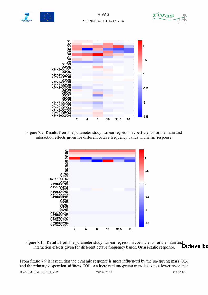
The result of the parametric study separated into the analysis of dynamic and quasi-static response is presented in figures 7.9 and 7.10 respectively. The linear regression coefficients in this case describe the effect of a parameter variation on the average vibration response at 0-2 m distance from the track. The result is presented in octave bands in the 2-63 Hz range and the parameters are represented by their coded variable presented in table 7.3. Two parameters separated by a * denotes an interaction between the parameters. A + in between two interaction effects means that there is a confounding between the effects which is a consequence of the simplified FFD.

RIVAS

SCP0-GA-2010-265754

RIVAS_UIC_ WP5_D5_1_V02 of 53 29/09/2011

2 4 8 16 31.5 63

X1X2X3X4X5X6X7X8X9

X1*X5X2*X5

X2*X6+X1*X7X3*X5

X3*X6+X1*X8X3*X7+X2*X8

X4*X5X4*X6+X1*X9X4*X7+X2*X9X4*X8+X3*X9

X4*X9X5*X6X5*X7X5*X8X5*X9

X6*X7+X1*X2X6*X8+X1*X3X6*X9+X1*X4X7*X8+X2*X3X7*X9+X2*X4X8*X9+X3*X4 -1.5

-1

-0.5

0

0.5

1

Figure 7.9. Results from the parameter study. Linear regression coefficients for the main and

interaction effects given for different octave frequency bands. Dynamic response.

2 4 8 16 31.5 63

X1X2X3X4X5X6X7X8X9

X1*X5X2*X5

X2*X6+X1+X7X3*X5

X3*X6+X1*X8X3*X7+X2*X8

X4*X5X4*X6+X1*X9X4*X7+X2*X9X4*X8+X3*X9

X4*X9X5*X6X5*X7X5*X8X5*X9

X6*X7+X1*X2X6*X8+X1*X3X6*X9+X1*X4X7*X8+X2*X3X7*X9+X2*X4X8*X9+X3*X4

-1.5

-1

-0.5

0

0.5

1

Figure 7.10. Results from the parameter study. Linear regression coefficients for the main and

interaction effects given for different octave frequency bands. Quasi-static response.

From figure 7.9 it is seen that the dynamic response is most influenced by the un-sprung mass (X3) and the primary suspension stiffness (X6). An increased un-sprung mass leads to a lower resonance

RIVAS

SCP0-GA-2010-265754

RIVAS_UIC_ WP5_D5_1_V02 of 53 29/09/2011

of the wheel on the track and hence a slight improvement is seen in the highest octave band. The effect of changing the suspension stiffness is concentrated to the frequency range containing the resonance of the bogie frame mass on the primary suspension. The same is true for an increased bogie frame mass. The carbody mass is uncoupled from the system through the secondary suspension already at a few Hz. Hence no influence is seen from this parameter above the 4 Hz octave band.

The result in figure 7.10 shows how the quasi-static response is governed primarily by the total axle load of the vehicle. An increase of the carbody mass according to table 7.3 gives the largest relative increase to the entire axle load and hence is seen most clearly in the ground vibration response. Changing the axle spacing or the distance between adjacent bogies will change the fundamental frequency of the periodic excitation that discrete axle loads give rise to.

RIVAS

SCP0-GA-2010-265754

RIVAS_UIC_ WP5_D5_1_V02 of 53 29/09/2011

7.3 SBB MEASUREMENTS PRATELN, THUN, LIGERTZ If nothing else is stated, pictures, results and conclusions in the following section are taken from reference [24].

The Swiss Federal Railway SBB has conducted extensive measurement campaigns in order to investigate the rolling stock influence on ground vibrations from the railway. The background to this is the future introduction of a more stringent environmental legislation which forces the railway to address its vibration problems. It is estimated that the necessary mitigation measures, if applied on the infrastructure, would cost more than 1 billion Euros in order to meet the future requirements. By investigating possible measures applied to the rolling stock instead of the infrastructure SBB hopes to find more cost efficient abatement methods.

Monitoring measurements were carried out at three different sites during several weeks which resulted in data of several hundred passing trains. The rolling stock consisted of a mix of freight trains travelling at approximately 75 km/h and regional and intercity trains travelling at about 100 km/h. The setup measured the vertical vibration response of the ground at 8 metres from the track centre line excited by the passing trains.

A selection of interesting results are presented and commented in the following section.

Figure 7.11 and 7.12 present two different statistical analyses of the vibration data from about 400 trains. Figure 7.11 gives the distribution of the vRMS,MAX value [mm/s] of the entire train passage separated into different vehicle categories. It can be seen that even though travelling at a lower speed, the freight trains (GZ) give rise to the largest vibration amplitudes followed by the intercity (IC) trains and the regional (RZ) trains.

Figure 7.11 Distribution of the vRMS,MAX value [mm/s] at 8 m from the track centre line for passages

of about 400 freight (GZ), regional (RZ) and intercity (IC) trains.

RIVAS

SCP0-GA-2010-265754

RIVAS_UIC_ WP5_D5_1_V02 of 53 29/09/2011

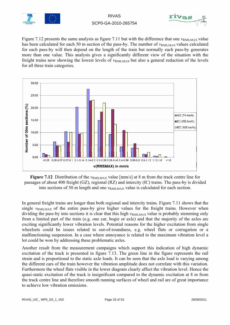
Figure 7.12 presents the same analysis as figure 7.11 but with the difference that one vRMS,MAX value has been calculated for each 50 m section of the pass-by. The number of vRMS,MAX values calculated for each pass-by will then depend on the length of the train but normally each pass-by generates more than one value. This analysis gives a significantly different view of the situation with the freight trains now showing the lowest levels of vRMS,MAX but also a general reduction of the levels for all three train categories.

Figure 7.12 Distribution of the vRMS,MAX value [mm/s] at 8 m from the track centre line for

passages of about 400 freight (GZ), regional (RZ) and intercity (IC) trains. The pass-by is divided into sections of 50 m length and one vRMS,MAX value is calculated for each section.

In general freight trains are longer than both regional and intercity trains. Figure 7.11 shows that the single vRMS,MAX of the entire pass-by give higher values for the freight trains. However when dividing the pass-by into sections it is clear that this high vRMS,MAX value is probably stemming only from a limited part of the train (e.g. one car, bogie or axle) and that the majority of the axles are exciting significantly lower vibration levels. Potential reasons for the higher excitation from single wheelsets could be issues related to out-of-roundness, e.g. wheel flats or corrugation or a malfunctioning suspension. In a case where annoyance is related to the maximum vibration level a lot could be won by addressing these problematic axles.

Another result from the measurement campaigns which support this indication of high dynamic excitation of the track is presented in figure 7.13. The green line in the figure represents the rail strain and is proportional to the static axle loads. It can be seen that the axle load is varying among the different cars of the train however the vibration amplitude does not correlate with this variation. Furthermore the wheel flats visible in the lower diagram clearly affect the vibration level. Hence the quasi-static excitation of the track is insignificant compared to the dynamic excitation at 8 m from the track centre line and therefore smooth running surfaces of wheel and rail are of great importance to achieve low vibration emissions.

RIVAS

SCP0-GA-2010-265754

RIVAS_UIC_ WP5_D5_1_V02 of 53 29/09/2011

Figure 7.13 Vibration amplitude [mm/s] from pass-by of two freight trains; one without wheel flats and one with clearly visible wheel flats. The green lines represent the rail strain and is proportional

to the static axle load of the train.

With the purpose of eliminating the influence of the ground an analysis was done by using a reference vehicle. In this case the average vibration spectrum of the intercity train was used as a reference and a difference in dB-level was calculated to the spectra of the regional trains and the freight trains. The result is presented in figure 7.14 and reveals some effects linked to the different vehicle designs.

The lack of a secondary suspension leads to the excitation of higher low frequency vibration levels from the freight train. This is seen below 10 Hz where the carbody mass of the regional train is decoupled already from a few Hz. The carbody mass of the freight train is however first uncoupled together with the bogie frame mass through the stiffer primary suspension at around 10 Hz. From 80 Hz the level of the freight spectrum is increasing significantly. One potential reason for this is the cast iron block brakes which tend to roughen the wheel tread [13]. The relevance of frequencies above 100 Hz for ground vibration can however be questioned. These frequencies lie more in the range of structure and air-borne noise which also have been proven to increase substantially by the use of cast iron block brakes [25]. In fact, in [25] a comparison between the roughnesses of wheels with different braking systems is made which shows an increased roughness level for the cast iron block braked wheel in the 5-20 cm wavelength range. Considering the speed of the freight train in the actual measurements this corresponds to the frequency range of 100-340 Hz in which the significant increase can be seen in figure 7.14.

RIVAS

SCP0-GA-2010-265754

RIVAS_UIC_ WP5_D5_1_V02 of 53 29/09/2011

Figure 7.14 Vertical vibration levels at 8 m from the track centre line. 1/3-octave spectra of freight

(GZ) and regional (RZ) trains presented as a delta to the average intercity train. The speed of the vehicles: freight 74 km/h, regional 106 km/h and intercity 100 km/h.

In order to relate the differences seen in figure 7.14 to the absolute vibration level in the ground, figure 7.15 gives the vibration velocity pass-by spectra of the different vehicle categories. The ground response shows a clear peak in the 60-80 Hz range independently of the speed and vehicle type. Hence this peak is related to the propagation properties of the ground and is most probably caused by the cut-on of propagating modes in the upper layer of soil [2,7]. The frequency of the peak is related to the stiffness of the soil and is more commonly seen at lower frequencies around 10-15 Hz. This implies that the soil on the test site in Switzerland is rather stiff which leads to the shift of the ground response towards higher frequencies. The maximum level of the spectrum, excited by the regional train (MP1), rises approximately 10 dB above the rest of the spectrum. At peak level, between 60 and 80 Hz the difference between the different vehicles is roughly 2 dB. Hence the influence of vehicle type is inferior to the influence of the ground response. Furthermore the differences seen between vehicle types in figure 7.14 (regarding the secondary suspension and the braking system) fall outside the range of maximum ground response. It is therefore likely to believe that these differences are of less importance at this particular site.

RIVAS

SCP0-GA-2010-265754

RIVAS_UIC_ WP5_D5_1_V02 of 53 29/09/2011

Figure 7.15 Pass-by vibration spectra for different vehicle categories measured in two positions,

both at 8 m from the track centre line.

RIVAS

SCP0-GA-2010-265754

RIVAS_UIC_ WP5_D5_1_V02 of 53 29/09/2011

8. PREDICTION MODELS

8.1 AVAILABLE PREDICTION MODELS AND PREDICTION RESULTS

Several models have been developed for the prediction of ground vibration generated by surface trains. Many of these models only take into account the vibration generated by moving axle loads (quasi-static loads). However, it has been demonstrated that the contribution to ground vibrations due to dynamic wheel–rail contact forces caused by wheel/rail irregularities and spatial variation of track stiffness may be as important as, or even more important than, the contribution due to quasi-static loads [7]. Two models, TGV and TRAFFIC, accounting for the influence of both quasi-static and dynamic excitations, will be described below. In both models, the ground vibration problem is solved in the frequency-wavenumber domain, prescribing the use of linear models of vehicle, track and wheel/rail contact.

In parallel, brief descriptions of numerical models dedicated for prediction of vehicle dynamics and wheel–rail interaction in the time domain will be given. In these latter models, non-linear wheel–rail contact, sometimes resulting in temporary loss of contact in the presence of wheel flats and insulation joints, and more complex vehicle models can be accounted for but the track and ground models are much simpler than in the TGV and TRAFFIC models. Two distinct classes of time-domain models will be mentioned: models devoted for simulation of low-frequency vehicle dynamics and models developed for prediction of high-frequency wheel–rail interaction and track dynamics. Since the objective of RIVAS WP5 is the optimization of vehicle properties in order to reduce ground vibration, a combination of the computer codes in the frequency and time domains may be an efficient approach.

For the perception of ground vibration, the frequency range of interest is often referred to as 5 – 80 Hz [2]. The vehicle, track and ground models in TGV and TRAFFIC are therefore adapted to be accurate in this frequency range. Vehicle models in commercial time-domain vehicle dynamics software are generally validated for frequencies up to about 20 Hz, whereas the interesting frequencies in high-frequency vehicle/track dynamics applications are in the interval from about 50 Hz up to a few kHz. Thus, in order to reach a mathematically consistent combination of the different computer codes, an adaptation of the vehicle/track models and frequency range in the time domain models is required.

8.1.1 TGV – Train Ground Vibration The TGV model, developed by ISVR in Southampton, UK, is described in [2,4,7,11]. The model includes three subsystems: vehicles, track and layered ground. It uses the moving axle loads and the vertical rail irregularities as inputs. The vehicles are represented by discretized mass-spring-damper systems, and the vertical dynamics of the vehicles are coupled to the track–ground model. The properties of the vehicles, track, soil and wheel–rail contacts (Hertz) are linearized. Receptances are determined for the vehicles and for the track on a layered ground at the wheel–rail contact points. Continuous wheel–rail contact is assumed. The vertical rail profile is decomposed into a spectrum of discrete harmonic components. Compatibility of displacements at the wheel–rail contact points couple the vehicles and the track–ground subsystems, and yield equations for the dynamic wheel–rail contact forces. Based on the superposition principle and Fourier transformations, a relationship between the power spectral density of the displacement (velocity and acceleration) power spectrum

RIVAS

SCP0-GA-2010-265754

RIVAS_UIC_ WP5_D5_1_V02 of 53 29/09/2011

of the ground surface (and/or track) and the vertical profile of the rails is derived. The response spectra of the ground surface are determined for a point that is stationary as the train moves past it. The influence of the quasi-static moving axle loads is added to the solution. The track–ground model is invariant in the direction of the rails, and thus vibration generated by variations in support stiffness along the track can not be covered. TGV is a FORTRAN 77 code. Further details of the vehicle, track and soil models in TGV are discussed in Sections 8.2.1, 8.3.1 and 8.4.1.

8.1.2 TRAFFIC The TRAFFIC model, developed by Katholieke Universiteit in Leuven, Belgium, is presented in [5,26]. The model accounts for the dynamic interaction between train, track and layered soil. The track is assumed to be invariant in the direction of the rail, which allows for an efficient solution in the frequency-wavenumber domain. The dynamic interaction problem is solved by means of a compliance (receptance) formulation in the frame of reference that moves with the vehicle. Continuous (linearized Hertzian) wheel–rail contact is assumed leading to a compatibility equation where the rail unevenness is considered. The vehicle is modelled as a multi-degree of freedom system, where the vehicle’s axles and car body are considered as rigid parts and the vehicle’s suspensions are represented by spring and damper elements. Each element Cv

kl of the vehicle compliance matrix represents the displacement at contact point k due to a unit impulse load at contact point l. Each element Ct

kl of the track compliance matrix represents the rail displacement at the time-dependent position of the kth axle due to a unit impulse load at the time-dependent position of the lth axle. Examples of the calculated direct track compliance are shown in Figure 8.1. The frequency content of the track unevenness is calculated from the wavenumber representation of the unevenness. As for TGV, the influence of variation in track support stiffness along the track is not considered. TRAFFIC is a MATLAB code. Further details of the vehicle, track and soil models in TRAFFIC are discussed in Sections 8.2.2, 8.3.2 and 8.4.2.

Figure 8.1 Example of direct track direct compliance (receptance) calculated in TRAFFIC. Three different train speeds: 0 km/h (dotted line), 218 km/h (dashed-dotted) and 294 km/h (solid). From

[26]

RIVAS

SCP0-GA-2010-265754

RIVAS_UIC_ WP5_D5_1_V02 of 53 29/09/2011

8.1.3 DIFF The DIFF model, developed by Chalmers University of Technology in Gothenburg, Sweden, is introduced in [15]. The dynamic train–track interaction is solved in the time domain. Non-linear vehicle and wheel–rail contact conditions can be considered, including situations involving loss of and recovered wheel–rail contact. The vehicle is represented by a discretized mass-spring-damper system. The track model is a finite element model with rigid boundaries at the rail ends and below the spring/damper model representing the ballast and soil. The influence of variation in track support stiffness along the track is considered. The solution is based on an extended state-space vector approach, and a complex-valued modal superposition for the linear track model with non-proportionally distributed damping. Constraint equations coupling the wheels and the rail are formulated accounting for the influence of a generic wheel/rail irregularity. DIFF is a MATLAB code. Further details of the vehicle and track models in DIFF are discussed in Sections 8.2.3, 8.3.3 and 8.4.3.

DIFF was developed for the simulation of high-frequency vehicle–track interaction in the frequency range from about 50 – 2000 Hz. Ground vibrations can not be calculated in DIFF as it does not contain a soil (half-space) model. However, DIFF may be useful in the RIVAS project as it provides a more qualitative model of the transient wheel–rail contact conditions in case of discrete wheel/rail irregularities such as wheel flats and insulation joints, it does not prescribe continuous wheel–rail contact, and variations in track support stiffness along the track model can be considered. The wheel–rail contact forces calculated in DIFF can be used as input to the TGV and TRAFFIC models. However, a prerequisite is that the direct and cross receptances of the vehicle and track models in DIFF are tuned with reasonable agreement to the corresponding receptances determined for the corresponding vehicle model and track model on layered soil in TGV/TRAFFIC.

8.1.4 SIMPACK – ADAMS – GENSYS – VAMPIRE – NUCARS There are several commercial computer codes tailored for the simulation of low-frequency vehicle dynamics. Examples of such software are listed in the heading of this paragraph. General dynamic vehicle–track interaction in three dimensions is solved in the time domain aiming to investigate vehicle performance such as curving behaviour, stability and comfort rather than ground vibration. The vehicle model is a multi-degree of freedom system including rigid bodies, flexible bodies, and linear and non-linear spring and damper elements. The frequency range of interest for vehicle dynamics is commonly up to about 20 Hz. The vehicle model is often validated by laboratory testing of individual suspension components and field testing of the complete vehicle, whereas the track model is very simple as discussed in Section 8.3.4.

Ground vibrations can not be calculated with these computer codes because of the simplified track model with reflective boundary conditions, and where there normally is no coupling of vibrations between adjacent wheelsets through the rail. However, these vehicle models may be the most suitable for optimization of vehicle components to reduce wheel–rail contact forces in the low-frequency range. The calculated wheel–rail contact forces can be used as input to the TGV and TRAFFIC models. However, as for DIFF, a prerequisite is an adaptation of the track and vehicle models in the commercial code.

RIVAS

SCP0-GA-2010-265754

RIVAS_UIC_ WP5_D5_1_V02 of 53 29/09/2011

8.2 VEHICLE MODELLING The text in this Section is an extract from [27] where several aspects of vehicle dynamics modelling are surveyed. The choice of model for the vehicle/track system depends on several aspects, such as purpose of simulations, frequency range of interest and access to relevant model data. For example, a less detailed vehicle model may be sufficient for preliminary studies and the secondary suspension may not require a very accurate model if the wheel-rail contact forces are the main interest. The traditional frequency range of interest in simulation of dynamic vehicle–track interaction is 0 – 20 Hz as this low frequency range covers the fundamental dynamics of the vehicle. This frequency range needs to be extended for an accurate calculation of ground vibration.

The main contribution to the generation of ground vibration is determined by the vertical wheel–rail contact forces (quasi-static and dynamic contributions). Thus, here the focus will be on vertical vehicle–track dynamics. This means that the number of degrees-of-freedom (dofs) in the vehicle model can be reduced.

A main subdivision of the vehicle components can be made into body components and suspension components. The body components include the car body, bogie frames and wheelsets. In many cases, the inertia properties of the bodies are of primary interest. However, in some applications, also the structural flexibility of the body needs to be considered. In particular this is true for the car body with several eigenmodes in the frequency range up to 20 Hz. The main suspension components are various physical springs and dampers whose forces are related to the displacements and velocities at the positions where the body and suspension components are connected.

In railway vehicle dynamics simulations it is desirable to represent the car body structural flexibility by only a limited number of dofs in addition to the rigid body dofs. The most common way of finding such a representation is to use the eigenmodes of the car body. The car body vibrations are promoted by a low damping of the car body structure. In coaches, insulation and other non-metallic interior materials can increase the relative damping to approximately 2 %. Passengers can also provide the system with additional damping, say up to 4 %.

The most common bogie type worldwide, the three-piece bogie, consists of three bodies. However, for a bogie frame that can be seen as a one-piece metal structure, the assumption of essentially rigid body behaviour is fair in most applications. Different braking equipment is often attached to the bogie frame. Such equipment may be merged with the bogie frame in the modelling process. For powered bogies, the traction motors are usually mainly supported by the bogie frame. In certain applications, the motors may be considered as separate bodies suspended in the bogie frame. The traction gear housing is also often partly supported by the bogie frame.

A typical mass for a plain wheelset is 1000 to 1500 kg. Additional mass can be introduced through brake discs and traction gear. The axle boxes also add mass but they should not be considered in calculating the wheelset pitch moment of inertia. Wheelsets are often modelled as rigid bodies, but wheel axle flexibility may affect the vehicle-track interaction. Axle bending can significantly alter the dynamic part of the wheel-rail forces. The lowest eigenfrequencies in bending for a free wheelset may be below 60 Hz, but more normally below 80 Hz. In particular for slender wheelsets, the structural flexibility should be reflected in the modelling. The relative damping of these modes is typically below 1 %.

Common suspension components are coil springs, leaf springs, rubber springs, air springs, friction dampers and hydraulic dampers. They play important roles in reducing bogie frame and car body accelerations as well as the dynamic wheel–rail contact forces. For wheel–rail contact excitation at frequencies above about 20 Hz, the dynamic behaviour of car body and bogies is decoupled from

RIVAS

SCP0-GA-2010-265754

RIVAS_UIC_ WP5_D5_1_V02 of 53 29/09/2011

the wheelsets by the primary and secondary suspensions. Since ground vibration models are generally executed in the frequency domain, the often complex behaviour of suspension components needs to be linearized.

The static behaviour of the spring types listed above can be determined through component measurements by slowly loading and unloading these components. The vertical tangent stiffness of a coil spring is virtually independent of the static load, whereas the air spring stiffness increases almost linearly with increasing preload. Rubber and leaf spring stiffnesses also often increase with increasing preload. When unloading the coil spring the corresponding force-displacement graph will almost coincide with that of the loading phase. Thus, the energy dissipation or hysteresis is very small. In contrast, the leaf spring undergoes significant hysteresis due to the sliding motions between the leaves. The air spring and rubber springs also experience some hysteresis due to internal friction-like mechanisms of the rubber parts.

If, for a given displacement amplitude, the frequency of excitation is increased the force-displacement graphs of both leaf springs and coil springs show very little difference. However, for rubber springs and air springs the viscous effects are significant thus suggesting frequency-dependent models. The classic model of a linear spring in parallel with a linear viscous damper (Kelvin model) is sufficient provided that the frequency range of interest is limited. For a wider frequency range, this model provides a too strong frequency dependence, leading to a significant dynamic stiffness at high frequencies. One common approach to overcome this is to add a spring in series with the dashpot. To provide an accurate model of the suspension characteristics in the frequency range of interest for ground vibration, a viscoelastic model involving several sets of springs and viscous dampers may even be adopted but then requires a number of additional input parameters.

Generally, all modelling features discussed in this Section can be considered when commercial vehicle dynamics software, such as SIMPACK, ADAMS, GENSYS, VAMPIRE and NUCARS are employed.

8.2.1 Vehicle models in TGV As only the vertical dynamics of the vehicle is considered, each body in the vehicle model has only two degrees-of-freedom (vertical displacement of its mass centre and its pitch motion). To enable analysis in the frequency domain, each non-linear suspension and/or wheel–rail contact is linearized. As a result, the differential equations of motion for the vehicle are linear and with constant coefficients, and is specified by a mass matrix and a stiffness matrix. Damping is introduced and included in the stiffness matrix, thus the elements of the stiffness matrix may be complex and frequency-dependent. The wheel–rail contact forces on the two rails are not separated. Receptances (displacement amplitude of the jth wheelset due to a unit vertical harmonic load of frequency Ω exerted at the kth wheelset) between the different wheelsets of the vehicle model are calculated.

The mass and stiffness matrices for three different types of vehicle are derived in [2]. One vehicle type represents a passenger coach with both primary and secondary suspensions, see Figure 8.2. Suspension models in TGV include the classic Kelvin model and a three-parameter model. However, a frequency-dependent suspension of any type can be considered. The hysteretic damping may also be incorporated by introducing a complex-valued spring stiffness. The (complex) stiffness of a primary suspension per axle is denoted by k1, and that of a secondary suspension per bogie is denoted by k2. For different types of suspension, k1 and k2 are different functions of frequency,

RIVAS

SCP0-GA-2010-265754

RIVAS_UIC_ WP5_D5_1_V02 of 53 29/09/2011

stiffness and damping of the suspension. Two configurations of the suspension model including spring stiffness and viscous damping are illustrated in Figure 8.3(a,b). Hysteretic damping can be incorporated into the suspension by introducing complex spring stiffness. The symbol in Figure 8.3(c) is used to represent a suspension of any type.

Other vehicle models available in TGV include a four-axle freight vehicle model with only one level of suspension installed between the car body and the bogies, and a two-axle freight vehicle model with suspension between wheelset and car body.

Figure 8.2 Model of vehicle with two bogies in TGV. From [2]

Figure 8.3 Different models of suspension in TGV. From [2]

8.2.2 Vehicle models in TRAFFIC The vehicle is modelled as a multi-dof rigid body system, where the vehicle’s axles and car body are considered as rigid parts and the vehicle’s suspension is represented by spring and damper elements. Linearized Hertzian wheel–rail contact is assumed. The vehicle’s equations of motion are written in a general form, making a distinction between the displacements of the body (car body, bogies, …), of the axles and at the vehicle–track contact points.

RIVAS

SCP0-GA-2010-265754

RIVAS_UIC_ WP5_D5_1_V02 of 53 29/09/2011

8.2.3 Vehicle models in DIFF The vertical dynamics of the vehicle is modelled as a multi-dof rigid body system in a similar procedure as in TGV and TRAFFIC. One example of a vehicle model is illustrated in Figure 8.4. An arbitrary number of adjacent vehicle models representing a train can be accounted for but the finite length of the track model needs to be considered, see Section 8.3.3. The secondary suspension acts as a low-pass filter isolating the car body from the bogie at frequencies above a few Hz. Thus, the weight of the car body is accounted for by a static load acting at the centre of gravity of the bogie mass. The wheelsets are modelled as rigid or as flexible using Craig-Bampton modes. Non-linear wheel–rail contact according to Hertz is considered.

Figure 8.4 Model of vehicle with one bogie in DIFF. The weight of half the car body is added as a

static load applied at the centre of gravity of the bogie mass

8.3 TRACK MODELS

8.3.1 TGV The layered track model in TGV, see Figure 8.5, is described in [10]. The railway track is infinite in length and is aligned in the x-direction. The two rails are modelled as a single Euler-Bernoulli beam with mass per unit length of track mR and bending stiffness EI. The sleepers are modelled as a distributed mass mS per unit length of track. The rail pads are represented as a distributed vertical spring stiffness kP between the rail beam and the sleeper mass. The discrete supports of the rail are neglected. The ballast is modelled as a viscoelastic layer with width 2b (which is also the contact width with the ground model) and a consistent mass approximation per unit length mB. For the ballast layer, only the vertical stiffness KB is taken into account. All track components are attributed damping properties by the use of complex stiffness parameters derived from a real-valued stiffness value and an associated loss factor η.

The axle loads are considered to be distributed through the ballast and possible embankment so that the wheel loading function applying to the ground surface is smooth. This assumption is inherent in the treatment of the track as having continuous distributed stiffness and mass.

RIVAS

SCP0-GA-2010-265754

RIVAS_UIC_ WP5_D5_1_V02 of 53 29/09/2011

Figure 8.5 Track model in TGV software. From [10]

8.3.2 TRAFFIC The track model in TRAFFIC (and in TGV) is assumed to be located at the surface of a horizontally layered and longitudinally invariant half-space. The model is continuous neglecting the discrete supports. The rails are modelled as Euler-Bernoulli beams with bending stiffness ErIr and mass ρrAr per unit length. The positions of the rails are determined by l1 and l2, see Figure 8.6. The rail pads are modelled as continuous spring-damper connections. The rail pad stiffness krp and viscous damping coefficient crp of a single rail pad are used to calculate an equivalent stiffness krp/d and damping crp/d in the continuous model where d is the sleeper distance. The sleepers are assumed to be rigid so that the vertical sleeper displacements along the track are determined by the vertical displacement at the centre of gravity of the sleeper and the rotation about this centre. The sleepers are assumed not to contribute to the longitudinal stiffness of the track so that they can be modelled as a uniformly distributed mass along the track. The sleeper mass msl is used to calculate a uniformly distributed mass msl/d per unit length. The width 2b of the track–soil interface is taken equal to the sleeper length lsl.

The ballast bed is assumed to act as a set of distributed independent linear springs and dampers (Winkler foundation). Each sleeper is supported by that part of the ballast that is in contact with the sleeper. The sleeper is assumed to be supported only under the rails. This means that the vertical spring stiffness per sleeper [N/m] is calculated from the effective support length esl per rail, the sleeper width bsl and the ballast bed modulus Kb [(N/m)/m2] as 2eslbslKb. The smeared ballast stiffness [(N/m)/m] is equal to kb/d. When viscous damping in the ballast bed is accounted for, the ballast dynamic stiffness equals bb ciω+k . In a similar way, the discrete support of the sleepers and the effective width determine the part of the ballast mass that is coupled to the sleepers and soil. The track–soil interface is assumed to be rigid in the plane of the track cross-section.

RIVAS

SCP0-GA-2010-265754

RIVAS_UIC_ WP5_D5_1_V02 of 53 29/09/2011

Figure 8.6 Cross-section of ballasted track model in TRAFFIC. From [26]

8.3.3 DIFF An example of the time-domain vehicle–track model DIFF is illustrated in Figure 8.7. In this case, the vehicle is represented by two wheelsets travelling along the track at constant speed (cf Figure 8.4).

The track model is a linear finite element (FE) model containing rail, rail pads, sleepers and ballast/subgrade. The rail is discretely supported and modelled by Euler-Bernoulli or Rayleigh-Timoshenko beam finite elements with bending stiffness EI, shear stiffness kGA, mass per unit beam length m and rotational inertia per unit beam length mr2. The number of rail elements per sleeper bay is 16. The sleepers are also modelled using beam theory. The length of the track model is typically up to 90 sleeper bays with sleeper spacing L and clamped boundaries at the two rail ends. Structural and loading symmetry are assumed with respect to an imaginary track centre-line, and hence it is sufficient to only incorporate half of the full track and half of the vehicle in the model. Only vibration in the vertical plane is studied.

The rail pads and the ballast may be modelled by 4-parameter viscoelastic models (i.e. two spring-damper sets coupled in series, with each set containing one spring and one viscous damper coupled in parallel, kp1, cp1, kp2, cp2, kub1, cub1, kub2, cub2). The track model in Figure 8.7 may be extended with a layer of rigid ballast masses. Each ballast mass is connected to the sleeper above via an additional layer of springs and dampers, and to the adjacent pair of ballast masses via springs and dampers acting in shear.

RIVAS

SCP0-GA-2010-265754

RIVAS_UIC_ WP5_D5_1_V02 of 53 29/09/2011

kub1, cub1

kH kp2, cp2

kub2, cub2

kp1, cp1

Fstat

v Mw

kw cw mw

Figure 8.7 Example of track model in DIFF. From [28]

8.3.4 GENSYS An example of a track model in GENSYS is illustrated in Figure 8.8. The track model is based on a co-following mass-spring-damper system that is coupled to each wheelset in the vehicle model (moving track model). There is no interaction between wheelsets through the track. In Figure 8.8, each track model consists of two rails with neglected inertia that are attached to one track mass by spring-damper elements in the lateral and vertical directions to account for the dynamic stiffness of rails and rail pads. The remaining track flexibility is represented by spring-damper elements that connect the track mass to a rigid ground. The properties of the moving track model may be time-variant to account for variations in track stiffness.

Figure 8.8 Example of track model in GENSYS. From [39]

RIVAS

SCP0-GA-2010-265754

RIVAS_UIC_ WP5_D5_1_V02 of 53 29/09/2011

8.4 GROUND MODELS

8.4.1 TGV The ground is modelled as n parallel viscoelastic layers overlying an elastic half-space or a rigid foundation (layer n+1). The material constants of layer j are the Young’s modulus Ej, Poisson ratio νj, density ρj, loss factor ηj and thickness hj. If layer n+1 is a half-space, its material constants are En+1, νn+1, ρn+1 and ηn+1. The differential equations of the ground are Navier’s equations. Transfer matrices relating the stresses and displacements at the top and bottom of a layer or at the surface of a half-space are used to model the complete multi-layered half-space. The coupling of the ground and track models is carried out by taking into account the continuity of displacements and the equilibrium of stresses in the plane of contact between them.

8.4.2 TRAFFIC A boundary element method is used to calculate the soil traction at the track–soil interface. The boundary element formulation is based on the boundary integral equations in the frequency-wavenumber domain, using the Green’s functions of a horizontally layered soil. Each layer in the half-space model is characterized by its thickness h, the dynamic soil characteristics E and ν or the longitudinal and transversal wave velocities Cp and Cs, the material density ρ and a material damping ratio βp and βs in volumetric and deviatoric deformation, respectively.

8.4.3 DIFF There is no ground model in DIFF. Rigid boundaries are assumed below the ballast/subgrade stiffness layer, see Figure 8.7.

8.4.4 GENSYS There is no ground model in GENSYS. Rigid boundaries are assumed below the track mass (trc), see Figure 8.8.

RIVAS

SCP0-GA-2010-265754

RIVAS_UIC_ WP5_D5_1_V02 of 53 29/09/2011

8.5 INPUT DATA Examples of input data for the track and ground models are given in Tables 8.1-8.3.

Table 8.1 Examples of sets of input data for ground model. From [4]

Table 8.2 Examples of sets of input data for track model. From [4]

RIVAS

SCP0-GA-2010-265754

RIVAS_UIC_ WP5_D5_1_V02 of 53 29/09/2011

Table 8.3 Examples of sets of input data for ground model. From [26]

8.5.1 Track irregularities For the perception of ground vibration, the frequency range of interest is often referred to as 5 – 80 Hz [2]. For a vehicle speed range of 36 – 250 km/h (10 – 70 m/s), the corresponding range of wheel/rail irregularities generating the dynamic excitation is 0.125 – 14 m.

A typical input for the simulation of ground vibration is the vertical (long-wavelength) track irregularity as regularly (on several occasions per year) measured by a track geometry recording car. To provide input for the complete range of irregularity wavelengths, the track geometry recording car measurements may need to be complemented with measurements of shorter wavelength irregularities by for example a trolley (corrugation analysis trolley or similar). Other irregularity inputs are idealised discrete events, such as wheel flats, dipped rail joints and crossings. All these track irregularity inputs can be studied in the computer codes discussed above. In TGV and TRAFFIC, the irregularity profile is decomposed into a spectrum of discrete harmonic components.

The influence of track stiffness irregularities, as caused by for example poor track tamping, hanging sleepers and transition zones, on wheel–rail contact forces can be studied in the time-domain models but not in TGV and TRAFFIC.

RIVAS

SCP0-GA-2010-265754

RIVAS_UIC_ WP5_D5_1_V02 of 53 29/09/2011

9. CONCLUDING REMARKS AND TOPICS FOR FUTURE RESEARCH

Considering dynamic and quasi-static excitation of the wheel-rail contact patch, a number of vehicle parameters may influence the magnitude and frequency content of the excitation. This is true for the entire range of excitation from lower frequencies important for ground vibrations and ground-borne noise to higher frequencies holding air-borne noise. When considering ground vibrations and also ground-borne noise the ground properties will be of significant influence for the propagation and may vary substantially from one location to the next. Good ground conditions will therefore constitute a major prerequisite in order to reach low vibration levels. Without a vehicle however there would be no excitation of the track and hence an optimal vehicle design in terms of reduced excitation of low frequency vibrations should also be considered a crucial factor in the pursuit of reduced ground vibrations.

As always, when introducing new design and performance requirements these must be achieved without jeopardizing the compliance with already existing requirements. Furthermore a hierarchy among the different requirements will always be present which will determine the priority and attention a specific design target will be given. On an existing vehicle, bogie parameters such as the mass of the wheelset and the bogie frame or the stiffness and damping of the suspension are optimized in order to meet requirements on ride comfort and stability as well as gauging. When modifying the vehicle with respect to reduced ground vibrations it must therefore be assured that the changes do not conflict with the performance in these areas.

The root cause of the dynamic excitation is the wheel and rail imperfections (and the stiffness variations along the track) which can take the form of long wavelength rail misalignments or wheel out-of-roundness, or discrete discontinuities such as rail joints, switches, wheel flats or other local wheel tread defects. Preventing and mitigating the existence and growth of these would be beneficial from several points of view such as noise and vibration emissions, comfort and wear. A relationship between the use of cast iron block-brakes and wheel corrugation has been established however there may be more connections between the growth of wheel and rail defects and vehicle design yet to be revealed. Especially if future work proves wheel OOR to be a significant cause of ground vibration the mapping of such correlations could constitute a major mitigation measure for ground vibration emissions.

One important step forward in the assessment of ground vibration emissions would be to relate the vibration levels and frequency content to vehicle speed, axle load and the size and shape of the wheel tread defect. Current limit values on tread defects and contact forces are related to the risk of wheel and rail damage. These should be assessed for their relevance for ground vibration and new, better suited limits should be proposed.

The only straightforward mitigation measures pointed out in the reviewed simulation work are the general reduction of axle load and wheel and rail imperfections. The axle load on a nominal track and with a perfect wheel will however only affect the quasi-static load which usually is important only close to the track. In the presence of wheel imperfections, e.g. a wheel flat, the wheel load will affect also the dynamic excitation which leads to propagating waves in the ground. This has not been investigated in the present studies and will be a topic for further research. The variation of other important parameters such as the un-sprung mass and the primary suspension stiffness leads to a frequency shift of the vehicle receptance. This shift must be viewed together with the track receptance and the frequency content of the wheel and rail imperfections in order to determine its potential to reduce vibrations. The use of several reference tracks/grounds with different properties

RIVAS

SCP0-GA-2010-265754

RIVAS_UIC_ WP5_D5_1_V02 of 53 29/09/2011

and running simulations at different speeds should enable a more comprehensive description of the problem.

The current parameter studies will be extended to include a more complex vehicle model. Non-linearity, a more accurate geometry and flexural motion of vehicle bodies are examples of effects which could be included if they are proven to be significant. The overall approach of new parametric studies will incorporate vehicle receptance calculations in a vehicle dynamics software like SIMPACK or GENSYS which will be used as input to a software including a more comprehensive ground model. In addition to allowing more complex vehicle models the use of a vehicle dynamics software for vehicle modeling will make it easier to study the impact on e.g. ride comfort or gauging since these predictions are done with the same software. The layered ground models are frequency domain models which include the excitation from wheel and rail irregularities as an input spectrum. The excitation from non-harmonic irregularities e.g. wheel flats or dents will be calculated in the time domain model DIFF. The resulting contact force time history will be frequency analyzed and used as input to the track and ground model.

The RIVAS project aims at finding cost efficient solutions with a high acceptance from rolling stock manufacturers and infrastructure managers. All possible measures resulting from the project must therefore be ranked and valued for their likelihood to be widely adopted. According to the very rough qualification of different measures done by SBB the highest benefit-to-cost ratio is achieved by addressing maintenance work and measures on already existing vehicles. In terms of probability of implementation, measures on new rolling stock are however more likely to be realized. Considering the 20-30 year life-cycle of a railway vehicle it is obvious that in order to achieve a reduction in ground vibration level from the railway in general, within a reasonable time frame, it will be necessary to develop efficient abatement methods for retrofit on existing vehicles.

RIVAS

SCP0-GA-2010-265754

RIVAS_UIC_ WP5_D5_1_V02 of 53 29/09/2011

10. REFERENCES

[1] RENVIB II Phase 1 – UIC Railway Vibration Project, State of the Art Review. J G Walker, G S Paddan and M J Griffin, 1997.

[2] X. Sheng, C.J.C. Jones, D.J. Thompson, A theoretical model for ground vibration from trains generated by vertical track irregularities, Journal of Sound and Vibration 272(3‐5) (2004) 937‐965.

[3] Railway noise and vibration – Mechanisms, modeling and means of control. David Thompson, 2009, ISBN‐13: 978‐0‐08‐045147‐3.

[4] X. Sheng, C.J.C. Jones, D.J. Thompson, A theoretical study on the influence of the track on train‐induced ground vibration, Journal of Sound and Vibration 272(3‐5) (2004) 909‐936.

[5] G. Lombaert, G. Degrande, Ground‐borne vibration due to static and dynamic axle loads of InterCity and high‐speed trains, Journal of Sound and Vibration 319 (2009) 1036‐1066.

[6] M. Heckle et al., Structure‐borne Sound and Vibration from Rail Traffic. Journal of Sound and Vibration (1996) 193(1), 175‐184.

[7] X. Sheng, C.J.C. Jones, D.J. Thompson, A comparison of a theoretical model for quasi‐statically and dynamically induced environmental vibration from trains with measurements, Journal of Sound and Vibration 267(3) (2003) 621‐635.

[8] L. Auersch, The excitation of ground vibration by rail traffic: theory of vehicle‐track‐soil interaction and measurements on high‐speed lines. Journal of Sound and Vibration (2005) 284, 103‐132.

[9] Noise and Vibration from High‐Speed Trains. 2001, Edited by Victor V Krylov. ISBN 0 7277 2963 2

[10] X. Sheng, C.J.C. Jones, M. Petyt, Ground vibration generated by a load moving along a railway track. Journal of Sound and Vibration (199) 288(1), 129‐156.

[11] C.J.C. Jones, X. Sheng, D.J. Thompson, The roles of track roughness and axle‐load time history in the generation of ground vibration from surface‐running trains. Structural Dynamics, EURODYN2002 Grundmann & Schueller 2002, ISBN 90 509 510

[12] J C O Nielsen, A Johansson Out‐of‐round railway wheels – a literature survey. Proceedings Institution Mechanical Engineers Vol 214 Part F, 2000.

[13] Vernersson, T. Thermally Induced roughness of tread braked railway wheels. Part 1: brake rig experiments, Wear 236, 96‐105, 1999.

[14] A. Johansson Out‐of‐Round Railway Wheels – Assessment of Wheel Tread Irregularities in Train Traffic. Part if PhD Thesis: Out‐of‐Round Railway Wheels – Causes and Consequences. Calmers. Department of Applies Mechanics 2005, ISBN91‐7291‐641‐9

[15] J C O Nielsen, A Igeland, Vertical dynamic interaction between train and track – influence of wheel and track imperfections. Journal of Sound and Vibration 187(5) (1995) 825‐839.

RIVAS

SCP0-GA-2010-265754

RIVAS_UIC_ WP5_D5_1_V02 of 53 29/09/2011

[16] A. Johansson, J.C.O. Nielsen, Out‐of‐round railway wheels – wheel‐rail contact forces and track response derived from field tests and numerical simulations. Journal of Rail and Rapid Transit 217 Part F.

[17] P. Torstensson, J.C.O. Nielsen, On the influence of wheel structural dynamics and the effects of wheel rotation on vertical wheel‐rail contact forces. Research report 2010:09, Chalmers department of applied mechanics, 2010.

[18] EN 15131 ‐ Railway application – In‐service wheelsets operation requirements – In‐service and off‐vehicle wheelset maintenance.

[19] J.C.O Nielsen Out-of-round railway wheels. Wheel/Rail Interface Handbook (editors R Lewis and U Olofsson), Woodhead Publishing, Cambridge (UK), pp. 245-279.

[20] R. Mueller, Initial study on mitigation measures for rolling stock, SBB. Presentation communicated via e-mail on 2011-09-19

[21] RENVIB II Pahse 2 Task 6 ‐ UIC Railway Vibration Project, Influences on the generation or Railway Ground‐borne Vibration AEAT 1999—03. B.P. Temple, J.R. Block.

[22] A. Mirza, A. Frid, J.C.O. Nielsen. Ground vibration induced by railway traffic – a pre‐study on the influence of vehicle parameters (Markvibrationer från järnvägstrafik – en förstudie med inriktning på inverkan av fordonsparametrar) Research report 2010:08. Chalmers, department of applied mechanics, 2010.

[23] Triepaischajonsak, N., Thompson, D.J., Jones, C.J.C., Ryue, J., Priest, J.A. Ground vibration from trains: experimental parameter characterisation and validation of a numerical model, to be published in Proceedings of Institution of Mechanical Engineers, Part F.

[24] R. Mueller. Measurement of rolling stock influence on railway vibrations and an overview of rolling stock mitigation measures. Railway environmental centre, SBB. Presented at Eurodyn Lueven, Belgium 2011.

[25] P.C. Dings, M.G. Dittrich, Roughness on Dutch Railway Wheel and Rails, Journal of Sound and Vibration 193(1) (1996) 103‐112.

[26] G. Lombaert, G. Degrande, J. Kogut, S. Francois, The experimental validation of a numerical model for the prediction of railway induced vibrations, Journal of Sound and Vibration 297 (2006) 512‐535.

[27] O. Polach, M. Berg, S. Iwnicki, Simulation, in: S. Iwnicki (Ed.), Handbook of Railway Vehicle Dynamics, Taylor & Francis, Boca Raton, 2006, pp. 359‐421.

[28] A Johansson, J C O Nielsen, R Bolmsvik, A Karlström, R Lundén, Under sleeper pads – influence on dynamic train–track interaction. Wear 265 (2008) 1479‐1487.

[29] I Persson, Using GENSYS.0803, ISBN 91‐631‐3112‐9, AB DEsolver, 2008

http://publications.lib.chalmers.se/cpl/record/index.xsql?pubid=111671

Train Induced Ground Vibration – Influence of Rolling...

Documents

Transcript of Train Induced Ground Vibration – Influence of Rolling...