Traian€E.€Abrudan,€Jan€Eriksson,€and€Visa€Koivunen.€2008...
15
Traian E. Abrudan, Jan Eriksson, and Visa Koivunen. 2008. Steepest descent algorithms for optimization under unitary matrix constraint. IEEE Transactions on Signal Processing, volume 56, number 3, pages 1134-1147. © 2008 IEEE Reprinted with permission. This material is posted here with permission of the IEEE. Such permission of the IEEE does not in any way imply IEEE endorsement of any of Helsinki University of Technology's products or services. Internal or personal use of this material is permitted. However, permission to reprint/republish this material for advertising or promotional purposes or for creating new collective works for resale or redistribution must be obtained from the IEEE by writing to [email protected]. By choosing to view this document, you agree to all provisions of the copyright laws protecting it.
Transcript of Traian€E.€Abrudan,€Jan€Eriksson,€and€Visa€Koivunen.€2008...

Traian E. Abrudan, Jan Eriksson, and Visa Koivunen. 2008. Steepest descent algorithmsfor optimization under unitary matrix constraint. IEEE Transactions on SignalProcessing, volume 56, number 3, pages 11341147.
© 2008 IEEE
Reprinted with permission.
This material is posted here with permission of the IEEE. Such permission of the IEEEdoes not in any way imply IEEE endorsement of any of Helsinki University ofTechnology's products or services. Internal or personal use of this material is permitted.However, permission to reprint/republish this material for advertising or promotionalpurposes or for creating new collective works for resale or redistribution must beobtained from the IEEE by writing to pubs[email protected].
By choosing to view this document, you agree to all provisions of the copyright lawsprotecting it.

1134 IEEE TRANSACTIONS ON SIGNAL PROCESSING, VOL. 56, NO. 3, MARCH 2008
Steepest Descent Algorithms for Optimization UnderUnitary Matrix Constraint
Traian E. Abrudan, Student Member, IEEE, Jan Eriksson, Member, IEEE, and Visa Koivunen, Senior Member, IEEE
Abstract—In many engineering applications we deal with con-strained optimization problems with respect to complex-valuedmatrices. This paper proposes a Riemannian geometry ap-proach for optimization of a real-valued cost function ofcomplex-valued matrix argument W, under the constraint thatW is an unitary matrix. We derive steepest descent(SD) algorithms on the Lie group of unitary matrices ( ).The proposed algorithms move towards the optimum along thegeodesics, but other alternatives are also considered. We alsoaddress the computational complexity and the numerical stabilityissues considering both the geodesic and the nongeodesic SDalgorithms. Armijo step size [1] adaptation rule is used similarlyto [2], but with reduced complexity. The theoretical results arevalidated by computer simulations. The proposed algorithms areapplied to blind source separation in MIMO systems by using thejoint diagonalization approach [3]. We show that the proposedalgorithms outperform other widely used algorithms.
Index Terms—Array processing, optimization, source separa-tion, subspace estimation, unitary matrix constraint.
I. INTRODUCTION
CONSTRAINED optimization problems arise in many
signal processing applications. One common task is to
minimize a cost function with respect to a matrix, under the con-
straint that the matrix has orthonormal columns. Some typical
applications in communications and array signal processing are
subspace tracking [4]–[6], blind and constrained beamforming
[7]–[9], high-resolution direction finding (e.g., MUSIC and
ESPRIT), and generally all subspace-based methods. Another
straightforward application is the independent component anal-
ysis (ICA), [3], [10]–[19]. This type of optimization problem
has also been considered in the context of multiple-input mul-
tiple-output (MIMO) communication systems [6], [20]–[23].
Most of the existing optimization algorithms are derived for the
real-valued case and orthogonal matrices [10], [11], [13]–[15],
[17], [24]–[27]. Very often in communications and signal pro-
cessing applications we are dealing with complex matrices and
signals. Consequently, the optimization need to be performed
under unitary matrix constraint.
Commonly optimization algorithms employing orthog-
onal/unitary matrix constraint minimize a cost function on
Manuscript received January 30, 2007; revised August 13, 2007. The as-sociate editor coordinating the review of this manuscript and approving it forpublication was Dr. Sergiy Vorobyov. This work was supported in part by theAcademy of Finland and by the GETA Graduate School.
The authors are with the SMARAD CoE, Signal Processing Laboratory, De-partment of Electrical Engineering, Helsinki University of Technology, FIN-02015 HUT, Finland (e-mail: [email protected]; [email protected];[email protected]).
Digital Object Identifier 10.1109/TSP.2007.908999
the space of matrices using a classical steepest descent
(SD) algorithm. Separate orthogonalization procedure must
be applied after each iteration [12], [20]–[22]. Approaches
stemming from the Lagrange multipliers method have also
been used to solve such problems [16]. In such approaches,
the error criterion contains an extra term that penalizes for
the deviations from orthogonality property. Self-stabilized
algorithms have been developed to provide more accurate, but
still approximate solutions [17]. Major improvements over the
classical methods are obtained by taking into account the geo-
metrical aspects of the optimization problem. Pioneering work
by Luenberger [28] and Gabay [29] convert the constrained
optimization problem into an unconstrained problem, on an
appropriate differentiable manifold. An extensive treatment of
optimization algorithms with orthogonality constraints is given
later by Edelman et al. [24] in a Riemannian geometry context.
A non-Riemannian approach has been proposed in [2], which
is a general framework for optimization under unitary matrix
constraint. A more-detailed literature review is presented in
Section II.
In this paper we derive two generic algorithms stemming
from differential geometry. They optimize a real-valued cost
function with respect to complex-valued matrix sat-
isfying , i.e., perform optimization sub-
ject to the unitary matrix constraint. SD algorithms operating
on the Lie group of unitary matrices are proposed. They
move towards the optimum along the locally shortest paths, i.e.,
geodesics. Geodesics on Riemannian manifolds correspond to
the straight lines in Euclidean space. Our motivation to opt for
the geodesic algorithms is that on the Lie group of unitary ma-
trices , the geodesics have simple expressions described by
the exponential map. We can fully exploit recent developments
in computing the matrix exponential needed in the multiplica-
tive update on . The generalized polar decomposition [30]
proves to be one of the most computationally efficient method if
implemented in a parallel architecture, or the Cayley transform
(CT) [31] otherwise. We also consider other parametrizations
proposed in the literature and show that all these parametriza-
tions are numerically equivalent up to a certain approximation
order. However, the algorithms differ in terms of computational
complexity, which is also addressed in this paper. The proposed
generic geodesic algorithms, unlike other parametrizations, can
be relatively easily adapted to different problems with varying
complexity and strictness of the unitarity property requirements.
This is due the fact that the computation of the matrix exponen-
tial function employed in the proposed algorithms is a well-re-
searched problem [32] with some recent progress relevant to
the unitary optimization [30]. Moreover, we show that the expo-
1053-587X/$25.00 © 2008 IEEE
ABRUDAN et al.: SD ALGORITHMS FOR OPTIMIZATION 1135
nential map is well suited for adapting the step size for the SD
method on the unitary group.
This paper is organized as follows. In Section II, an overview
of the problem of optimization under unitary matrix constraint is
provided. A brief review of different approaches presented in the
literature is given as well. A simple geometric example is used
to illustrate the differences among various approaches. In Sec-
tion III, we derive the Riemannian gradient on the Lie group of
unitary matrices and the corresponding SD algorithms. Equiva-
lence relationships between the proposed algorithms and other
algorithms are established in Section IV. The computational
complexity and the numerical stability issues are studied in Sec-
tions V and VI, respectively. Simulation results are presented in
Section VII. The proposed algorithms are used to solve the uni-
tary matrix optimization problem encountered in the joint ap-
proximate diagonalization of eigenmatrices (JADE) algorithm
[3] which is applied for blind source separation in a MIMO
system. Finally, Section VIII concludes the paper.
II. OPTIMIZATION UNDER UNITARY MATRIX CONSTRAINT
In this section, a brief overview of optimization methods
under orthonormal or unitary matrix constraint is provided. Dif-
ferent approaches are reviewed and the key properties of each
approach are briefly studied. A simple example is presented to
illustrate how each algorithm searches for the optimum.
A. Overview
Most of classical optimization methods with unitary matrix
constraint operate on the Euclidean space by using a SD algo-
rithm. The unitary property of the matrix is lost in every itera-
tion, and it needs to be restored in each step. Moreover, the con-
vergence speed is reduced. Other algorithms use a Lagrangian
type of optimization, by adding an extra-penalty function which
penalizes for the deviation from unitarity [16]. These methods
suffer from slow convergence and find only an approximate
solution in terms of orthonormality. Self-stabilized algorithms
provide more accurate solutions [17], [33].
A major drawback of the classical Euclidean SD and La-
grange type of algorithms [12], [16], [20]–[22] is that they do
not take into account the special structure of the parameter space
where the cost function needs to be optimized. The constrained
optimization problem may be formulated as an unconstrained
one in a different parameter space called manifold. Therefore,
the space of unitary matrices is considered to be a “constrained
surface.” Optimizing a cost function on a manifold is often con-
sidered [10], [14], [24], [25], [29], [34] as a problem of Rie-
mannian geometry [35]. Algorithms more general than the tra-
ditional Riemannian approach are considered in [2].
The second important aspect neglected in classical algorithms
is that the unitary matrices are algebraically closed under
the multiplication operation, not under addition. Therefore, they
form a group under the multiplication operation, which is the
Lie group of unitary matrices, [36]. Consequently,
by using an iterative algorithm based on an additive update the
unitarity property is lost after each iteration. Even though we
are moving along a straight line pointing in the right direction,
we depart from the constrained surface in each step. This hap-
pens because a Riemannian manifold is a “curved space.” The
locally length-minimizing curve between two points on the Rie-
mannian manifold is called a geodesic and it is not a straight
line like on the Euclidean space. Several authors [10], [11], [13],
[14], [24], [25], [28], [29], [34], [37], [38] have proposed that the
search for the optimum should proceed along the geodesics of
the constrained surface. Relevant work in Riemannian optimiza-
tion algorithms may be found in [24], [29], [34], and [38]–[41].
Algorithms considering the real-valued Stiefel and/or Grass-
mann manifolds have been proposed in [10], [11], [15], [17],
[24]–[26], and [42]. Edelman et al. [24] consider the problem of
optimization under orthonormal constraints. They propose SD,
conjugate gradient, and Newton algorithms along geodesics on
Stiefel and Grassman manifolds.
A general framework for optimization under unitary matrix
constraints is presented in [2]. It is not following the traditional
Riemannian optimization approach. A modified SD algorithm,
coupled with Armijo’s step size adaptation rule [1] and a
modified Newton algorithm are proposed for optimization on
both the complex Stiefel and the complex Grassmann mani-
fold. These algorithms do not employ a geodesic motion, but
geodesic motion could be used in the general framework. A
local parametrization based on an Euclidean projection of the
tangent space onto the manifold is used in [2]. Hence, the
computational cost may be reduced. Moreover, it is suggested
that the geodesic motion is not the only solution, since there
is no direct connection between the Riemannian geometry of
the Stiefel (or Grassmann) manifold (i.e., the “constrained
surface”) and an arbitrary cost function.
The SD algorithms proposed in this paper operate on the
Lie group of unitary matrices . We have derived the
Riemannian gradient needed in the optimization on . We
choose to follow a geodesic motion. This is justified by the
desirable property of that the right multiplication is an
isometry with respect to the canonical bi-invariant metric [35].
This allows us to translate the descent direction at any point
in the group to the identity element and exploit the fact that
the tangent space at identity is the Lie algebra of skew-Hermi-
tian matrices. This leads to lower computational complexity
because the argument of the matrix exponential operation is
skew-Hermitian. Novel methods for computing the matrix
exponential operation for skew-symmetric matrices recently
proposed in [30] and [32] may be exploited. Moreover, we
show that using an adaptive step size according to Armijo’s
rule [1] fits very well to the proposed algorithms.
B. Illustrative Example
We present a rather simple simulation example, in order to il-
lustrate how different algorithms operate under the unitary con-
straint. We consider the Lie group of unit-norm complex num-
bers , which are the 1 1 unitary matrices. The unitary
constraint is in this case the unit circle. We minimize the cost
function , subject to . Five different
algorithms are considered. The first one is the unconstrained SD
algorithm on the Euclidean space, with the corresponding up-
date , where is the step size. The

1136 IEEE TRANSACTIONS ON SIGNAL PROCESSING, VOL. 56, NO. 3, MARCH 2008
Fig. 1. Minimization of a cost function on the unit circle U(1). Euclideanversus Riemannian SD methods.
second one is the same SD with enforcing the unit norm con-
straint, , after each iteration. The third
method is similar to the bigradient method [16] derived from
the Lagrange multiplier method. An extra-penalty
weighted by a parameter is added to the original cost function
in order to penalize the deviation from the unit norm. In
this case, . The
fourth SD algorithm operates on the right parameter space de-
termined by the constraint. At each point the algorithm takes
a direction tangent to the unit circle and the resulting point is
projected back to the unit circle. The corresponding update is
, where
is the step size and is the operator which projects an arbi-
trary point to the closest point on the unit circle in terms of Eu-
clidean norm. The fifth algorithm is a multiplicative update SD
algorithm derived in this paper. The corresponding update is a
rotation, i.e., , where
and is the imaginary part of . The parameter rep-
resents the step size. The starting point is for
all the algorithms (see Fig. 1). The point , sets
the cost function to its minimum , but this is an
undesired minimum because it does not satisfy the constraint.
The desired optimum is , where the constraint is
satisfied and . We may notice in Fig. 1 that
the unconstrained SD (marked by ) takes the SD direction in
, and goes straight to the undesired minimum. By enforcing
the unit norm constraint, we project radially the current point
on the unit circle . The enforcing is necessary at every itera-
tion in order to avoid the undesired minimum. The extra-penalty
SD algorithm follows the unconstrained SD in the first it-
eration, since initially the extra-penalty term is equal to zero.
It converges somewhere between the desired and the undesired
minimum.
The SD algorithm [2] on the space determined by the con-
straint takes in this case the SD direction on , tangent
to the unit circle. The resulting point is projected to the closest
point on the unit circle in terms of Euclidean norm. The pro-
posed SD algorithm uses a multiplicative update which
is a phase rotation. The phase is proportional to the imaginary
part of the complex number associated with the point. For this
reason, the constraint is satisfied at every step in a natural way.
Although this low-dimensional example is rather trivial, it has
been included for illustrative purposes. In the case of multidi-
mensional unitary matrices, a similar behavior is encountered.
III. ALGORITHM DERIVATION
In this section, we derive two generic SD algorithms on the
Lie group of unitary matrices. Consider a real-valued cost func-
tion of a complex matrix , i.e., . Our
goal is to minimize (or maximize) the function
under the constraint that , i.e., is uni-
tary. We proceed as follows. First, in Section III-A we describe
the Lie group of unitary matrices, which is a real
differentiable manifold. Moreover, we describe the real differ-
entiation of functions defined in complex spaces in a way which
is suitable for the optimization. In Section III-B, we introduce
the Riemannian metric on the Lie group . The definition of
the gradient on the Riemannian space is intimately related to this
metric. The Riemannian gradient is derived in Section III-C, and
a basic generic optimization algorithm is given in Section III-D.
Finally, a Riemannian SD algorithm with an adaptive step size
is given in Section III-E.
A. Differentiation of Functions Defined in Complex Spaces
A Lie group is defined to be a differentiable manifold with a
smooth, i.e., differentiable group structure [36]. The Lie group
of unitary matrices is a real differentiable manifold be-
cause it is endowed with a real differentiable structure. There-
fore, we deal with a real-valued cost function essentially defined
in a real parameter space. However, since the algebraic proper-
ties of the group are defined in terms of the complex field, it is
convenient to operate directly with complex representation of
the matrices instead of using separately their real and the imagi-
nary parts, i.e., without using reals for representing the complex
space [43], [44]. Now the real differentiation can be described
by a pair of complex-valued operators defined in terms of real
differentials with respect to real and imaginary parts [43], [45]
and
(1)
with and . If a function is holo-
morphic (analytical), the first differential operator in (1) coin-
cides with the complex differential and the second one is iden-
tically zero (Cauchy-Riemann equations). It should be noted
that a real-valued function is holomorphic only if it is a con-
stant. Therefore, the complex analyticity is irrelevant to opti-
mization problems. The above representation is more compact,
allows differentiation of complex argument functions without

ABRUDAN et al.: SD ALGORITHMS FOR OPTIMIZATION 1137
using reals for the representation, and it is appropriate for many
applications [45].
B. Riemannian Structure on
A differentiable function represents a
curve on the smooth manifold (see Fig. 2). Let
and let be the set of functions on that are differentiable
at . The tangent vector to the curve at is a function
given by
(2)
A tangent vector at is the tangent vector at of
some curve with . All the tangent vectors at a
point form the tangent space . The tangent
space is a real vector space attached to every point in the differ-
ential manifold. It should be noted that the value is
independent of the choice of local coordinates (chart) and inde-
pendent of the curve as long as and
[35]. Since the curve , we have .
Differentiating both sides with respect to , the tangent space
at may be identified with the -dimensional real
vector space (i.e., it is a vector space isomorphic to)
(3)
From (3), it follows that the tangent space of at the group
identity is the real Lie algebra of skew-Hermitian matrices
. We empha-
size that is not a complex vector space (Lie algebra),
because the skew-Hermitian matrices are not closed under
multiplication with complex scalars. For example, if is a
skew-Hermitian matrix, then is Hermitian. Let and be
two tangent vectors, i.e., . The inner product
in is given by
(4)
This inner product induces a bi-invariant Riemannian metric
on the Lie group [35]. We may define the normal space at
considering that is embedded in the ambient space
, equipped with the Euclidean metric. The normal space
is the orthogonal complement of the tangent space
with respect to the metric of the ambient space [24],
i.e., for any and , we have
. It follows that the normal
space at is given as
(5)
C. The SD Direction on the Riemannian Space
We consider a differentiable cost function .
Intuitively, the SD direction is defined as “the direction
where the cost function decreases the fastest per unit length.”
Having the Riemannian metric, we are now able to derive the
Riemannian gradient we are interested in. A tangent vector
Fig. 2. Illustrative example representing the tangent space T U(n) at pointW, and a tangent vector X 2 T U(n).
satisfying for all
the condition
(6)
is the gradient on evaluated at . The direction
defined in (1) represents the steepest ascent
direction of the cost function of complex argument on the
Euclidean space at a given [45]. The left-hand side (LHS) in
(6) represents an inner product in the ambient space, whereas the
right-hand side (RHS) represents a Riemannian inner product at
. Equation (6) may be written as
(7)
Equation (7) shows that the difference , is
orthogonal to all . Therefore, it lies in the normal
space (5), i.e.,
(8)
where the matrix is a Hermitian matrix determined by im-
posing the condition that . From (3) it follows
that:
(9)
From (8) and (9), we get the expression for the Hermitian matrix
. The gradient of the cost func-
tion on the Lie group of unitary matrices at may be written
by using (8) as follows:
(10)
D. Moving Towards the SD Direction in
Here, we introduce a generic Riemannian SD algorithm along
geodesics on the Lie group of unitary matrices . A geodesic
curve on a Riemannian manifold is defined as a curve for
which the second derivative is zero or it lies in the normal
space for all (i.e., the acceleration vector stays normal to the
direction of motion as long as the curve is traced with constant
speed). Locally the geodesics minimize the path length with re-
spect to the Riemannian metric ([35, p. 67]). A geodesic ema-
nating from the identity with a velocity is characterized by
the exponential map:
(11)

1138 IEEE TRANSACTIONS ON SIGNAL PROCESSING, VOL. 56, NO. 3, MARCH 2008
Fig. 3. The geodesic emanating from identity in the direction of �G ending at P = exp(��G ).
The exponential of complex matrices is given by the con-
vergent power series . The opti-
mization of is carried out along geodesics on the con-
straint surface. For the optimization we need the equation of the
geodesic emanating from . This may be found by
taking into account the fact that the right translation in is
an isometry with respect to the metric given by (4) and an isom-
etry maps geodesics to geodesics [10], [35]. Therefore,
. It follows that the geodesic emanating from is
, i.e.,
(12)
Consequently, we need to translate the gradient of the cost func-
tion at (10) to identity, i.e., into the Lie algebra . Since
the differential of the right translation is a vector space isomor-
phism, this is performed simply by postmultiplying
by , i.e.,
(13)
We have to keep in mind that this is not the Riemannian gradient
of the cost function evaluated at identity. The tangent vector
is the Riemannian gradient of the cost function evaluated
at and translated to identity. Note that the argument of the
matrix exponential operation is skew-Hermitian. We exploit this
very important property later in this paper in order to reduce the
computational complexity.
The cost function may be minimized iteratively by
using a geodesic motion. Typically we start at .
We choose the direction in to be the negative direction
of the gradient, i.e., (13). Moving from
to , is equivalent to moving
from to , as it is shown in Fig. 3. The geodesic motion
in corresponds to the multiplication by a rotation matrix
. The parameter controls the magni-
tude of the tangent vector and consequently the algorithm con-
vergence speed. The update corresponding to the SD algorithm
along geodesics on is given by
(14)
TABLE ITHE BASIC RIEMANNIAN SD ALGORITHM ON U(n)
The algorithm is summarized in Table I. Practical algorithms
require the computation of the exponential map, which is ad-
dressed in Section V.
E. A Self-Tuning Riemannian SD Algorithm on
An optimal value of the step size is difficult to determine
in practice. Moreover, it is cost function dependent and the ap-
propriate step size may change at each iteration. The SD algo-
rithm with a fixed small step size converges in general close to
a local minimum. It trades off between high convergence speed,
which requires large step size, and low steady-state error, which
requires a small step size. An adaptive step size is often a desir-
able choice.
In [27], a projection algorithm is considered together with
three other optimization alternatives along geodesics in the real
case, i.e., on the orthogonal group. The first geodesic algorithm
in [27] uses a fixed step size, which leads to the “real-valued
counterpart” of the algorithm in Table I. The second one is
a geodesic search for computing the step size in the update
equation. If the geodesic search is performed in a continuous
domain [39], [40], it is computationally very expensive since
it involves differential equations. A discretized version of the
geodesic search may be employed. Two such methods are re-
viewed in [27]. The third alternative is a stochastic type of algo-
rithm which adds perturbation to the search direction.
We opt for a fourth alternative based on the Armijo step size
[1]. It allows reducing the computational complexity and gives
the optimal local performance. This type of algorithm takes an
initial step along the geodesic. Then, two other possibilities are
checked by evaluating the cost function for the case of doubling
or halving the step size. The doubling or halving step continues

ABRUDAN et al.: SD ALGORITHMS FOR OPTIMIZATION 1139
TABLE IITHE SELF-TUNING RIEMANNIAN SD ALGORITHM ON U(n)
as long as the step size is out of a range whose limits are set by
two inequalities. It is known that in a stationary scenario (i.e.,
the matrices involved in the cost function are time invariant)
the SD algorithm together with the Armijo step size rule [1] al-
most always converges to a local minimum if not initialized at
a stationary point. The convergence properties of the geodesic
SD algorithm using the Armijo rule have been established in
[29], [46] for general Riemannian manifolds, provided that the
cost function is continuously differentiable and has bounded
level sets. The first condition is an underlying assumption in
this paper and the second one is ensured by the compactness
of .
In [2], a SD algorithm is coupled with the Armijo rule for op-
timizing the step size. Geodesic motion is not used. Neverthe-
less, in the general framework proposed in [2] it could be used.
We show that by using the Armijo rule together with the generic
SD algorithm along geodesics, the computational complexity is
reduced by exploiting the properties of the exponential map, as
it will be shown later.
The generic SD algorithm with adaptive step size selection is
summarized in Table II. The choice for computing the matrix
exponential is explained in Section V.
Algorithm Description: The algorithm consists of the fol-
lowing steps.
• Step 1—Initialization: A typical initial value is .
If the gradient , then the identity element is a
stationary point. In that case a different initial value
may be chosen.
• Steps 2–3—Gradient computation: The Euclidean gradient
and Riemannian gradient are computed.
• Step 4—Setting the threshold for the final error: Evaluate
the squared norm of the Riemannian gradient in
order to check if we are sufficiently close to the minimum
of the cost function. The residual error may be set to a
value closest to the smallest value available in the limited-
precision environment, or the highest value which can be
tolerated in task at hand.
• Step 5—Rotation matrix computation: This step requires
the computation of the rotation matrix .
The rotation matrix may be com-
puted just by squaring , because
. Therefore, when doubling the step size,
instead of computing a new matrix exponential only
a matrix squaring operation is needed. It is important
to mention that the squaring operation is a very stable
operation [32] being also used in software packages for
computing the matrix exponential.
• Steps 6 and 7—Step size evaluation: In every iteration we
check if the step size is in the appropriate range determined
by the two inequalities. The step size evolves in a dyadic
basis. If it is too small it will be doubled and if it is too high
it will be halved.
• Step 8—Update: The new update is obtained in a multi-
plicative manner and a new iteration is started with step 2
if the residual error is not sufficiently small.
Remark: The SD algorithm in Table II may be easily con-
verted into a steepest ascent algorithm. The only difference is
that the step size would be negative and the inequalities in
steps 6 and 7 need to be reversed.
IV. RELATIONS AMONG DIFFERENT LOCAL
PARAMETRIZATIONS ON THE UNITARY GROUP
The proposed SD algorithms search for the minimum bymoving along geodesics, i.e., the local parametrization is theexponential map. Other local parametrizations used to describea small neighborhood of a point in the group have been pro-posed in [2] and [11]. In this section, we establish equivalencerelationships among some different local parametrizations ofthe unitary group . The first one is the exponential mapused in the proposed SD algorithms, the second one is theCayley transform [31], the third one is the Euclidean projectionoperator [2], and the fourth one is a parametrization basedon the QR-decomposition. The four parametrizations lead todifferent update rules for the basic SD algorithm on . Theupdate expressions may be described in terms of Taylor seriesexpansion, and we prove the equivalence among all of them upto a certain approximation order.
A. The Exponential Map
The rotation matrix used in the update expression (14)of the proposed algorithm can be expressed as a Taylor seriesexpansion of the matrix exponential, i.e.,
. The update isequivalent to
(15)
B. The Cayley Transform
If the rotation matrix in the update is computed by usingthe CT [31] instead of the matrix exponential, then
. The corresponding Taylor series is. For the update equation is
(16)Obviously, (16) is equivalent to (15) up to the second order.Notice also that for the CT equals the first order

1140 IEEE TRANSACTIONS ON SIGNAL PROCESSING, VOL. 56, NO. 3, MARCH 2008
diagonal Padé approximation of (i.e., ,see [32]).
C. The Euclidean Projection Map
Another possibility is to use an Euclidean projection map asa local parametrization as in [2]. This map projects an arbi-trary matrix onto at a point which is theclosest point to in terms of Euclidean norm, i.e.,
. The unitary matrixminimizing the above norm can be obtained from the polar de-composition of as in [47]
(17)
where and are the left and the right singular vectors of, respectively. Equivalently
(18)
Equation (18) is also known as “the symmetric orthogonaliza-tion” procedure [12]. In [2], the local parametrizations are moregeneral in the sense that they are chosen for the Stiefel andGrassmann manifolds. The projection operation is computed viaSVD as in (17). For the SD algorithm on the Stiefel manifold [2],the update is of form , where is theSD direction on the manifold and is the step size. According to(18) the update is equivalent to
. By expanding the above expressionin a Taylor series we get
(19)Considering that and , forthe three update expressions (15), (16), and (19) become equiv-alent up to the second order.
D. The Projection Based on the QR-Decomposition
A computationally inexpensive way to approximate the op-timal projection of an arbitrary matrix onto (18) is theQR-decomposition. We show that this is not the optimal pro-jection in terms of minimum Euclidean distance, but is accu-rate enough to be used in practical applications. We establisha connection between the QR-based projection and the optimalprojection. Let us consider the QR-decomposition of the arbi-trary nonsingular matrix given bywhere is an upper triangular matrix and is a unitary ma-trix. The unitary matrix is an approximation of the optimalprojection of onto , i.e., . The connec-tion between this projection and the optimal projection can beestablished by using the polar decomposition of the upper-trian-gular matrix . We obtain ,where and . There-fore, the matrix is an approximation of the optimal pro-jection and it includes an additional rotation from
. The update of the SD algorithm is equal to the unitaryfactor from the QR-decomposition. In other words, if we have
, then
(20)
The equivalence up to the first order between the update (20) andthe other update expressions (15), (16), and (19) is obtained byexpanding the columns of the matrix from the Gram-Schmidt process separately in a Taylor series (proof availableon request)
(21)
The equivalence may extend to higher orders, but this remainsto be studied.
V. COMPUTATIONAL COMPLEXITY
In this section, we evaluate the computational complexity ofthe SD algorithms on by considering separately the the
geodesic and the nongeodesic SD algorithms. The proposedgeodesic SD algorithms use the rotational update of form
, and the rotation matrix is computedvia matrix exponential. We review the variety of algorithmsavailable in the literature for calculating the matrix exponentialin the proposed algorithms. Details are given for the matrixexponential algorithms with the most appealing properties. Thenongeodesic SD algorithms are based on an update expressionof form , and the computationalcomplexity of different cases is described. The cost of adaptingto the step size using the Armijo rule is also evaluated. The SDmethod on involves overall complexity of flops1
per iteration. Algorithms like conjugate gradient or Newtonalgorithm are expected to provide a faster convergence, but alsotheir complexity is expected to be higher. Moreover, a Newtonalgorithm is more likely to converge to stationary points otherthan local minima.
A. Geodesic SD Algorithms on
In general, the geodesic motion on manifolds is computation-ally expensive. In the case of , the complexity is reducedeven though it requires the computation of the matrix exponen-tial. We are interested in the special case of matrix exponentialof form , where and is a skew-Hermi-tian matrix. Obviously, finding the exponential of a skew-Her-mitian matrix has lower complexity than of general matrix. Thematrix exponential operation maps the skew-Hermitian matricesfrom the Lie algebra into unitary matrices which reside onthe Lie group . Several alternatives for approximating thematrix exponential have been proposed in [30], [32], [48], and[49]. In general the term “approximation” may refer to two dif-ferent things. The first kind of approximation maps the elementsof the Lie algebra exactly into the Lie group, and the approxi-mation takes place only in terms of deviation “within the con-strained surface.” Among the most efficient methods from thiscategory are: the diagonal Padé approximation [32], General-ized Polar Decomposition [30], [48], technique of coordinatesof the second kind [49]. The second category includes methodsfor which the resulting elements do not reside on the group any-more, i.e., . The most popular methods belonging to
1One “flop” is defined as a complex addition or a complex multiplication. Anoperation of form ab+ c; a; b; c 2 is equivalent to two flops. A simple mul-tiplication of two n� n matrices requires 2n flops. This is a quick evaluationof the computational complexity, not necessarily proportional to the computa-tional speed.

ABRUDAN et al.: SD ALGORITHMS FOR OPTIMIZATION 1141
this category is the truncated Taylor series and the nondiagonalPadé approximation. They do not preserve the algebraic proper-ties, but they still provide reasonable performance in some ap-plications [50]. Their accuracy may be improved by using themtogether with the scaling and squaring procedure.
1) Padé Approximation of the Matrix Exponential: This is[32, Method 2], and together with scaling and squaring [32,Method 3] is considered to be one of the most efficient methodsfor approximating a matrix exponential. For normal matrices(i.e., matrices which satisfy ), the Padéapproximation prevents the round-off error accumulation. Theskew-Hermitian matrices are normal matrices, therefore, theyenjoy this benefit. Because we deal with a SD algorithm on
we are also concerned about preserving the Lie algebraicproperties. The diagonal Padé approximation preserves theunitarity property accurately. The Padé approximation togetherwith scaling and squaring supposes the choice of the Padéapproximation order and the scaling and squaring exponentto get the best approximant given the approximation accuracy.See [32] for information of choosing the pair optimally.The complexity of this approximation isflops. The drawback of Padé method when used together withthe scaling and squaring procedure is that if the norm of theargument is large the computational efficiency decreases due tothe repeated squaring.
2) Approximation of the Matrix Exponential via Generalized
Polar Decomposition (GPD): The GPD method, recently pro-posed in [30] is consistent with the Lie group structure as it mapsthe elements of the Lie algebra exactly into the correspondingLie group. The method lends itself to implementation in parallelarchitectures and it requires about flops [30] regardless ofthe approximation order. It may not be the most efficient imple-mentation in terms of flop count, but the algorithm has potentialfor highly parallel implementation. GPD algorithms based onsplitting techniques have also been proposed in [48]. The cor-responding approximation is less complex than the one in [30]for the second and the third order. The second-order approxima-tion requires only flops. This is the same amount ofcomputation needed to perform the CT. Other efficient approx-imations in a Lie-algebraic setting have been considered in [49]by using the technique of coordinates of the second kind (CSK).A second-order CSK approximant requires flops.
B. Nongeodesic SD Algorithms on
This category includes local parametrizations derived from aprojection operator which is used to map arbitrary matrices into
. The optimal projection and an approximation of it areconsidered.
1) Optimal Projection: The projection that minimizes theEuclidean distance between the arbitrary matrix and a matrix
may be computed in different ways. By using theSVD the computation of the projection requires flops andby using the procedure (18) it requires about flops.
2) Approximation of the Optimal Projection: This methodis the most inexpensive approximation of the optimal projec-tion, being based on the QR-decomposition of the matrix .It requires only the unitary matrix which is an orthonormal
TABLE IIITHE COMPLEXITY (IN FLOPS) OF COMPUTING THE LOCAL PARAMETRIZATION
IN U(n)
basis in the range space of . This can be done by using House-holder reflections, Givens rotations or the Gram-Schmidt proce-dure [32]. The most computationally efficient and numericallystable approach is the modified Gram-Schmidt procedure whichrequires only flops.
In Table III, we summarize the complexity2 of computingthe local parametrizations for the geodesic and the nongeodesicmethods, respectively. The geodesic methods include: the diag-onal Padé approximation with scaling and squaring
of type (1, 0) [32] (CT), the Generalized Polar Decom-position with reduction to tridiagonal form (GPD-IZ) [30] andwithout reduction to the tridiagonal form (GPD-ZMK) [48]. Allmethods have an approximation order of two. The nongeodesicmethods include the optimal projection (OP) and its approxima-tion (AOP).
C. The Cost of Using an Adaptive Step Size
In this subsection, we analyze the computational complexityof adapting the step size with Armijo rule. The total computa-tional cost is given by the complexity of computing the localparametrization and the additional complexity of selecting thestep size. Therefore, the step size adaptation is a critical aspectto be considered. We consider again the geodesic SD algorithmsand the nongeodesic SD algorithms, respectively. We show thatthe geodesic methods may reduce the complexity of the step sizeadaptation.
1) The Geodesic SD Algorithms: Since the step size evolvesin a dyadic basis, the geodesic methods are very suitable for theArmijo step. This is due to the fact that doubling the step sizedoes not require any expensive computation, just squaring therotation matrix as in the scaling and squaring procedure. Fornormal matrices, the computation of the matrix exponential viamatrix squaring prevents the round-off error accumulation [32].An Armijo type of geodesic SD algorithm enjoys this benefit,since the argument of the matrix exponential is skew-Hermitian.Moreover, when the step size is halved, the corresponding rota-tion matrix may be available from the scaling and squaring pro-cedure which is often combined with other methods for approx-imating the matrix exponential. This allows reducing the com-plexity because the expensive operation may often be avoided.
2) The Nongeodesic SD Algorithms: The nongeodesicmethods compute the update by projecting a matrix into .Unfortunately, the Armijo step size adaptation is relativelyexpensive in this case. The main reason is that the update
and the one corresponding to thedouble step size do not have astraightforward relationship as squaring the rotation matrix forthe geodesic methods. Thus, the projection operation needs tobe computed multiple times. Moreover, even keeping the stepsize constant involves the computation of the projection twice
2Only dominant terms are reported, i.e., O(n ).
1142 IEEE TRANSACTIONS ON SIGNAL PROCESSING, VOL. 56, NO. 3, MARCH 2008
TABLE IVTHE COMPLEXITY OF ADAPTING THE STEP SIZE
since both inequalities 6 and 7 in Table II need to be tested evenif they fail. In this case both projections and
need to be evaluated.We compare the proposed geodesic SD algorithms to the
nongeodesic SD algorithms by considering the complexity ofadapting to the step size. We also take into account the costof computing the rotation matrix for the geodesic SD algorithmsand the cost of computing the projection operation for thenongeodesic algorithms. These costs are given in Table III fordifferent local parametrizations. We denote by and thenumber of times we double, respectively, the number of timeswe halve the step size during one iteration . The complexityof adapting the step size is summarized in Table IV.
We may conclude that the local parametrization may bechosen based on the requirements of the application. Often,preserving the algebraic structure is important. On the otherhand, the implementation complexity may be a limiting factor.Most of the parametrizations presented here are equivalent upto the second order. Therefore, the difference in convergencespeed is not expected to be significant. The cost function tobe minimized plays a role in this difference as also stated in[2]. An SD algorithm with adaptive step size is more suitablein practice. Consequently, the geodesic algorithms are a goodchoice. In this case, the matrix exponential is employed and itmay be computed either by using the CT [31] or the GPD-ZMKmethod [48]. They require equal number of flops, thereforethe choice remains upon the numerical stability. Even thoughthe GPD-IZ method recently proposed in [30] is sensibly lessefficient in terms of flop count, it may be faster in practice ifimplemented in parallel architectures. Moreover, it providesgood numerical stability as it will be seen in the simulations.As a final conclusion, we would opt for the GPD-IZ method[30] if the algorithm is implemented in a parallel fashion andfor the CT if the parallel computation is not an option.
VI. NUMERICAL STABILITY
In this section, we focus on the numerical stability of the pro-posed SD algorithms on . Taking into account the recur-sive nature of the algorithms, we analyze the deviation of eachnew update from the unitary constraint, i.e., the depar-ture from . The nongeodesic SD algorithms do not experi-ence this problem due to nature of local parametrization. In thatcase, the error does not accumulate because the projection op-erator maps the update into the manifold at every new iteration.Therefore, we consider only the geodesic SD algorithms.
The methods proposed here for approximating the matrix ex-ponential map the elements of the Lie algebra exactly into theLie group, therefore they do not cause deviation from the uni-tary constraint. However, the rotation matrix may be affectedby round-off errors, and the error may accumulate in the update(14) due to the repeated matrix multiplications.
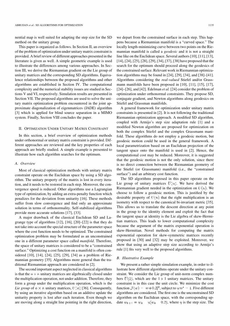
We provide a closed-form expression for the expected valueof the deviation form the unitary constraint after a certainnumber of iterations. The theoretical value derived here pre-dicts the error accumulation with high accuracy, as it will beshown in the simulations. We show that the error accumulationis negligible in practice.
We assume that at each iteration , the rotation matrixis affected additively by the quantization error , i.e.,
where is the true rotationmatrix. The real and imaginary parts of the entries of the matrix
are mutually independent and independent of the entry in-dices. They are assumed to be uniformly distributed within thequantization interval of width . The deviation of the quantizedupdate from the unitary constraint is measured by
(22)
The closed-form expression of the expected value of the devia-tion at iteration is given by (derivation available on request)
(23)
The theoretical value (23) depends on the matrix dimensionand the width of the quantization interval . Often, the conver-gence is reached in just few iterations, as in the practical ex-ample presented in Section VII. Therefore, the error accumula-tion problem is avoided. We show that even if the convergence isachieved after a large number of iterations, the expected valueof the deviation from the unitary constraint is negligible. Thisis due to the fact that the dominant term in (23) is driven bythe factor . The error is increasing very slowly and theincreasing rate decays rapidly with , as it will be shown in Sec-tion VII.
VII. SIMULATION RESULTS AND APPLICATIONS
In this section, we test how the proposed method performsin signal processing applications. An example of separating in-dependent signals in a MIMO system is given. Applications toarray signal processing, ICA, BSS, for MIMO systems may befound in [5]–[8], [10], [14]–[17], [19]–[23], [51]. A recent re-view of the applications of differential geometry to signal pro-cessing may be found in [52].
A. Blind Source Separation for MIMO Systems
Separating signals blindly in a MIMO communication sys-tems may be done by exploiting the statistical information ofthe transmitted signals. The JADE algorithm [3] is a reliablealternative for solving this problem. The JADE algorithm con-sists of two stages. First, a prewhitening of the received signal isperformed. The second stage is a unitary rotation. This secondstage is formulated as an optimization problem under unitarymatrix constraint, since no closed form solution can be given ex-cept for simple cases such as 2-by-2 unitary matrices. This maybe efficiently solved by using the proposed SD on the unitarygroup. It should be noted that the first stage can also be formu-lated as a unitary optimization problem [50], and the algorithms

ABRUDAN et al.: SD ALGORITHMS FOR OPTIMIZATION 1143
proposed in this paper could be used to solve it. However, herewe only focus on the second stage.
The JADE approach has been recently considered on theoblique [53] and Stiefel [19] manifolds. The SD algorithmin [19] has complexity of per iteration as the originalJADE [3], but in general it converges in fewer iterations. This istrue especially for large matrix dimensions, where JADE seemsto converge slowly due to its pairwise processing approach.Therefore, the overall complexity of algorithm in [19] is lowerthan in the original JADE. It operates on the Stiefel manifold of
unitary matrices, but still without taking into account theadditional Lie group structure of the manifold. Our proposedalgorithm is designed specifically for the case of unitarymatrices, and for this reason the complexity per iteration islower compared to the SD in [19]. The convergence speed isidentical as it will be shown later. The algorithms in [2] and[19] are more general than the proposed one, in the sense thatthe parametrization is chosen for the Stiefel and the Grassmannmanifolds. The reduction in complexity for the proposed algo-rithm is achieved by exploiting the additional group structureof . The SD along geodesics is more suitable for Armijostep size.
A number of independent zero-mean signals are sent byusing transmit antennas and they are received by receiveantennas. The frequency flat MIMO channel matrix is inthis case an mixing matrix . We use the clas-sical signal model used in source separation. The ma-trix corresponding to the received signal may be written as
where is an matrix corresponds tothe transmitted signals and is the additive white noise.In the prewhitening stage the received signal is decorrelatedbased on the eigendecomposition of the correlation matrix. The
prewhitened received signal is given by ,where and contain the eigenvectors and the eigen-values corresponding to the signal subspace, respectively.
In the second stage, the goal is to determine a unitary matrixsuch that the estimated signals are the transmitted
signals up to a phase and a permutation ambiguity, which are in-herent to any blind methods. The unitary matrix may be obtainedby exploiting the information provided by the fourth-order cu-mulants of the whitened signals. The JADE algorithm mini-mizes the following criterion:
(24)
with respect to , under the unitarity constraint on , i.e., wedeal with a minimization problem on . The eigenmatrices
which are estimated from the fourth-order cumulants needto be diagonalized. The operator computes the sum of thesquared magnitudes of the off-diagonal elements of a matrix,therefore, the criterion penalizes the departure of all eigenma-trices from the diagonal property. The Euclidean gradient of theJADE cost function is
, where denotes the elementwise matrix multi-plication.
The performance is studied in terms of convergence speedconsidering the JADE criterion and the Amari distance (perfor-mance index) [12]. This JADE criterion (24) is a measure of
Fig. 4. The constellation patterns corresponding to (a) four of the six receivedsignals and (b) the four recovered signals by using JADE with the algorithmproposed in Table I. There is an inherent phase ambiguity which may be noticedas a rotation of the constellation, as well as a permutation ambiguity.
how well the eigenmatrices are jointly diagonalized. Thischaracterizes the goodness of the optimization solution, i.e., theunitary rotation stage of the BSS. The Amari distance is agood performance measure for the entire blind source separa-tion problem since it is invariant to permutation and scaling. Interms of deviation from the unitary constraint the performanceis measured by using a unitarity criterion (22), in a logarithmicscale.
A number of signals are transmitted, three QPSK sig-nals and one BPSK signal. The signal-to-noise ratio (SNR) is
dB and the channel taps are independent randomcoefficients with power distributed according to a Rayleigh dis-tribution. The results are averaged over 100 random realizationsof the (4 6) MIMO matrix and (4 1000) signal matrix.
In the first simulation, we compare three optimization algo-rithms: the classical Euclidean SD algorithm which enforcesthe unitarity of after every iteration, the Euclidean SDwith extra-penalty similar to [16] stemming from the Lagrangemultipliers method and the proposed Riemannian SD algorithmfrom Table II. The update rule for the classical SD algorithmis . The unitarity property is enforcedby symmetric orthogonalization after every iteration [12], i.e.,
. The extra-penalty SD
method uses an additional termadded to the original cost function (24) similarly to the bi-gradient method in [16]. The corresponding update rule is
. Aweighting factor is used to weight the importance ofthe unitarity constraint. The third method is the SD algorithmsummarized in Table II. Armijo [1] step size selection rule isused for all four methods. Fig. 4 shows received signal mix-tures, and separated signals by using JADE with the proposedalgorithm. The performance of the three algorithms in termsof convergence speed and accuracy of satisfying the unitaryconstraint are presented in Fig. 5. The JADE criterion (24)versus the number of iterations is shown in subplot a) of Fig. 5.Subplot b) of Fig. 5 shows the evolution of the Amari distancewith the number of iterations. We may notice that the accuracyof the optimization solution described by the value of the JADEcost function is very related to the accuracy of solving the entiresource separation, i.e., the Amari distance. The Riemannian SDalgorithm (Table I) converges faster compared to the classical
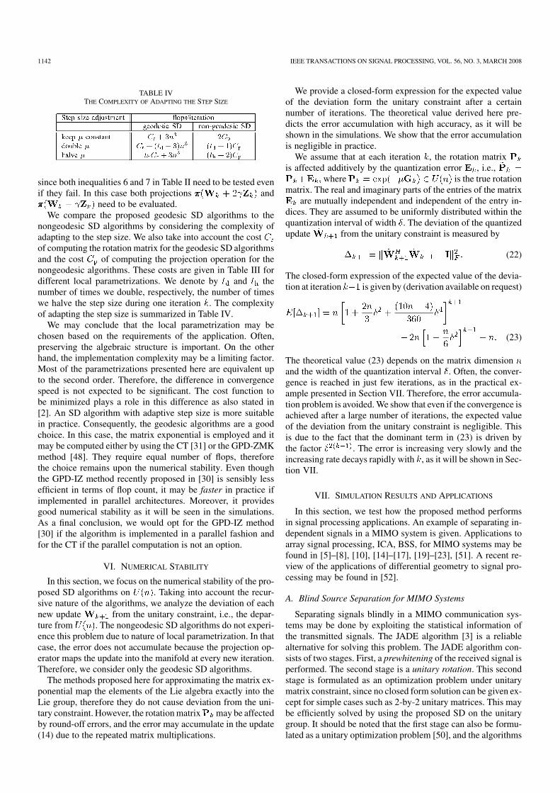
1144 IEEE TRANSACTIONS ON SIGNAL PROCESSING, VOL. 56, NO. 3, MARCH 2008
Fig. 5. A comparison between the conventional optimization methods oper-ating on the Euclidean space (the classical SD algorithm with enforcing uni-tarity, the extra-penalty SD method) and the Riemannian SD algorithm fromTable II. The horizontal thick dotted line in subplots (a) and (b) represents thesolution of the original JADE algorithm [3]. The performance measures are theJADE criterionJ (W )(24), Amari distance d and the unitarity criterion� (22) versus the iteration step. The Riemannian SD algorithm outperforms theconventional methods.
methods, i.e., the Euclidean SD with enforcing unitarity andthe extra-penalty method. The Euclidean SD and extra-penaltymethod do not operate in an appropriate parameter space, andthe convergence speed is decreased. All SD algorithms satisfyperfectly the unitary constraint, except for the extra-penaltymethod which achieves also the lowest convergence speed. Thisis due to the fact that an optimum scalar weighting parametermay not exist. The unitary matrix constraint is equivalent tosmooth real Lagrangian constrains, therefore more parameterscould be used. However, computing these parameters maycomputationally expensive and/or non-trivial even in the caseof , like the example presented in Section II-B. Theaccuracy of the solution in terms of unitary constraint is shownin subplot c) of Fig. 5 considering the criterion (22) versusthe number of iterations.
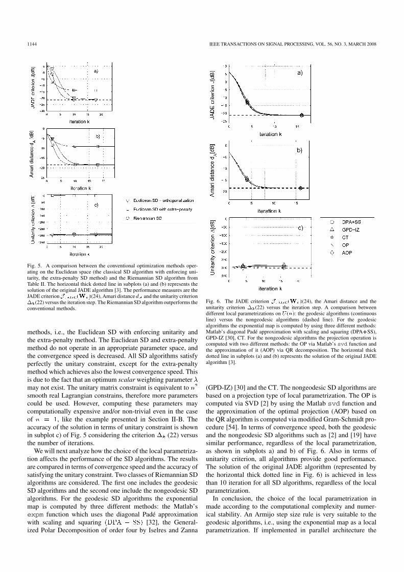
We will next analyze how the choice of the local parametriza-tion affects the performance of the SD algorithms. The resultsare compared in terms of convergence speed and the accuracy ofsatisfying the unitary constraint. Two classes of Riemannian SDalgorithms are considered. The first one includes the geodesicSD algorithms and the second one include the nongeodesic SDalgorithms. For the geodesic SD algorithms the exponentialmap is computed by three different methods: the Matlab’sexpm function which uses the diagonal Padé approximationwith scaling and squaring [32], the General-ized Polar Decomposition of order four by Iselres and Zanna
Fig. 6. The JADE criterion J (W )(24), the Amari distance and theunitarity criterion � (22) versus the iteration step. A comparison betweendifferent local parametrizations on U(n): the geodesic algorithms (continuousline) versus the nongeodesic algorithms (dashed line). For the geodesicalgorithms the exponential map is computed by using three different methods:Matlab’s diagonal Padé approximation with scaling and squaring (DPA+SS),GPD-IZ [30], CT. For the nongeodesic algorithms the projection operation iscomputed with two different methods: the OP via Matlab’s svd function andthe approximation of it (AOP) via QR decomposition. The horizontal thickdotted line in subplots (a) and (b) represents the solution of the original JADEalgorithm [3].
(GPD-IZ) [30] and the CT. The nongeodesic SD algorithms arebased on a projection type of local parametrization. The OP iscomputed via SVD [2] by using the Matlab svd function andthe approximation of the optimal projection (AOP) based onthe QR algorithm is computed via modified Gram-Schmidt pro-cedure [54]. In terms of convergence speed, both the geodesicand the nongeodesic SD algorithms such as [2] and [19] havesimilar performance, regardless of the local parametrization,as shown in subplots a) and b) of Fig. 6. Also in terms ofunitarity criterion, all algorithms provide good performance.The solution of the original JADE algorithm (represented bythe horizontal thick dotted line in Fig. 6) is achieved in lessthan 10 iteration for all SD algorithms, regardless of the localparametrization.
In conclusion, the choice of the local parametrization inmade according to the computational complexity and numer-ical stability. An Armijo step size rule is very suitable to thegeodesic algorithms, i.e., using the exponential map as a localparametrization. If implemented in parallel architecture the

ABRUDAN et al.: SD ALGORITHMS FOR OPTIMIZATION 1145
Fig. 7. The deviation from the unitary constraint for different values of thequantization errors � on the rotation matrices ~P after one million iterations.The theoretical value E[� ] in (23) is represented by continuous black line.The unitarity criterion � (22) obtained by repeatedly multiplying unitary ma-trices is represented by dashed gray line. The value � obtained by using theproposed SD algorithm in Table II is represented by dot-dashed thick black line.The theoretical expected value of the deviation from the unitary constraint pre-dicts accurately the value obtained in simulations. The proposed algorithm pro-duces an error lower that the theoretical bound due to the fact that the error doesnot accumulate after the convergence has been reached.
GPD-IZ method [30] for computing the matrix exponentialis a reliable choice from the point of view of efficiency andcomputational speed. Otherwise, the CT provides a reasonableperformance at a low computational cost. Finally, the proposedalgorithm has lower computational complexity per iterationcompared to the nongeodesic SD in [2], [19] at the sameconvergence speed. This reduction is achieved by exploitingthe Lie group structure of the Stiefel manifold of unitarymatrices.
The last simulation shows how the round-off errors causedby finite numerical precision affect the proposed iterative algo-rithm. In Fig. 7, different values of the quantization error areconsidered for the rotation matrices , which are obtained byusing the method [32]. Similar results are obtainedby using the other approximation methods of the matrix expo-nential presented in Section V-A. The theoretical value of theunitarity criterion in (23) is represented by continuouslines. The value (22) obtained by repeatedly multiplyingunitary matrices is represented by dashed lines and the valueobtained by using the proposed algorithm in Table II is repre-sented by dot-dashed thick lines. The theoretical value (23) pre-dicts accurately the value (22) obtained by repeated multiplica-tions of unitary matrices. The proposed algorithm exhibits anerror below the theoretical value due to the fact that the conver-gence is reached in few steps. Even if the convergence wouldbe reached after a much larger number of iterations, the erroraccumulation is negligible for reasonable values of the quanti-zation errors , as shown in Fig. 7. In practice, a muchsmaller number of iterations need to be performed.
VIII. CONCLUSION
In this paper, Riemannian optimization algorithms on the Lie
group of unitary matrices have been introduced.
Expression for Riemannian gradient needed in the optimization
has been derived. The proposed algorithms move towards the
optimum along geodesics and the local parametrization is the
exponential map. We exploit the recent developments in com-
puting the matrix exponential needed in the multiplicative up-
date on . This operation may be efficiently computed in a
parallel fashion by using the GPD-IZ method [30] or in a serial
fashion by using the CT. We also address the numerical issues
and show that the geodesic algorithms together with the Armijo
rule [1] are more efficient in practical implementations. Non-
geodesic algorithms have been considered as well, and equiva-
lence up to a certain approximation order has been established.
The proposed geodesic algorithms are suitable for practical
applications where a closed form solution does not exist, or to
refine estimates obtained by classical means. Such an example
is the joint diagonalization problem presented in the paper. We
have shown that the unitary matrix optimization problem en-
countered in the JADE approach for blind source separation
[3] may be efficiently solved by using the proposed algorithms.
Other possible applications include: smart antenna algorithms,
wireless communications, biomedical measurements and signal
separation, where unitary matrices play an important role in
general. The algorithms introduced in this paper provide sig-
nificant advantages over classical Euclidean gradient with en-
forcing unitary constraint and Lagrangian type of methods in
terms convergence speed and accuracy of the solution. The uni-
tary constraint is automatically maintained at each iteration, and
consequently, undesired suboptimal solutions may be avoided.
Moreover, for the specific case of , the proposed algorithm
has lower computational complexity than the nongeodesic SD
algorithms in [2].
REFERENCES
[1] E. Polak, Optimization: Algorithms and Consistent Approximations.
New York: Springer-Verlag, 1997.
[2] J. H. Manton, “Optimization algorithms exploiting unitary constraints,”
IEEE Trans. Signal Process., vol. 50, pp. 635–650, Mar. 2002.
[3] J. Cardoso and A. Souloumiac, “Blind beamforming for non Gaussian
signals,” Inst. Elect. Eng. Proc.-F, vol. 140, no. 6, pp. 362–370, 1993.
[4] S. T. Smith, “Subspace tracking with full rank updates,” in Conf. Rec.
31st Asilomar Conf. Signals, Syst. Comp., Nov. 2–5, 1997, vol. 1, pp.
793–797.
[5] D. R. Fuhrmann, “A geometric approach to subspace tracking,” in
Conf. Rec. 31st Asilomar Conf. Signals, Syst., Comp., Nov. 2–5, 1997,
vol. 1, pp. 783–787.
[6] J. Yang and D. B. Williams, “MIMO transmission subspace tracking
with low rate feedback,” in Int. Conf. Acoust., Speech Signal Process.,
Philadelphia, PA, Mar. 2005, vol. 3, pp. 405–408.
[7] W. Utschick and C. Brunner, “Efficient tracking and feedback of
DL-eigenbeams in WCDMA,” in Proc. 4th Europ. Pers. Mobile
Commun. Conf., Vienna, Austria, 2001.
[8] M. Wax and Y. Anu, “A new least squares approach to blind beam-
forming,” in IEEE Int. Conf. Acoust., Speech, Signal Process., Apr.
21–24, 1997, vol. 5, pp. 3477–3480.
[9] P. Stoica and D. A. Linebarger, “Optimization result for constrained
beamformer design,” in IEEE Signal Process. Lett., Apr. 1995, vol. 2,
pp. 66–67.
[10] Y. Nishimori, “Learning algorithm for independent component anal-
ysis by geodesic flows on orthogonal group,” in Int. Joint Conf. Neural
Netw., Jul. 10–16, 1999, vol. 2, pp. 933–938.
[11] Y. Nishimori and S. Akaho, “Learning algorithms utilizing
quasi-geodesic flows on the Stiefel manifold,” Neurocomputing,
vol. 67, pp. 106–135, Jun. 2005.

1146 IEEE TRANSACTIONS ON SIGNAL PROCESSING, VOL. 56, NO. 3, MARCH 2008
[12] A. Hyvärinen, J. Karhunen, and E. Oja, Independent Component Anal-
ysis. New York: Wiley, 2001.
[13] S. Fiori, A. Uncini, and F. Piazza, “Application of the MEC network
to principal component analysis and source separation,” in Proc. Int.
Conf. Artif. Neural Netw., 1997, pp. 571–576.
[14] M. D. Plumbley, “Geometrical methods for non-negative ICA: Man-
ifolds, Lie groups, toral subalgebras,” Neurocomput., vol. 67, pp.
161–197, 2005.
[15] A. Cichocki and S.-I. Amari, Adaptive Blind Signal and Image Pro-
cessing. New York: Wiley, 2002.
[16] L. Wang, J. Karhunen, and E. Oja, “A bigradient optimization approach
for robust PCA, MCA and source separation,” in Proc. IEEE Conf.
Neural Netw., 27 Nov.–1 Dec. 1995, vol. 4, pp. 1684–1689.
[17] S. C. Douglas, “Self-stabilized gradient algorithms for blind source
separation with orthogonality constraints,” IEEE Trans. Neural Netw.,
vol. 11, pp. 1490–1497, Nov. 2000.
[18] S.-I. Amari, “Natural gradient works efficiently in learning,” Neural
Comput., vol. 10, no. 2, pp. 251–276, 1998.
[19] M. Nikpour, J. H. Manton, and G. Hori, “Algorithms on the Stiefel
manifold for joint diagonalisation,” in Proc. IEEE Int. Conf. Acoust.,
Speech Signal Process., 2002, vol. 2, pp. 1481–1484.
[20] C. B. Papadias, “Globally convergent blind source separation based
on a multiuser kurtosis maximization criterion,” IEEE Trans. Signal
Process., vol. 48, pp. 3508–3519, Dec. 2000.
[21] P. Sansrimahachai, D. Ward, and A. Constantinides, “Multiple-input
multiple-output least-squares constant modulus algorithms,” in IEEE
Global Telecommun. Conf., Dec. 1–5, 2003, vol. 4, pp. 2084–2088.
[22] C. B. Papadias and A. M. Kuzminskiy, “Blind source separation with
randomized Gram-Schmidt orthogonalization for short burst systems,”
in Proc. IEEE Int. Conf. Acoust., Speech, Signal Process., May 17–21,
2004, vol. 5, pp. 809–812.
[23] J. Lu, T. N. Davidson, and Z. Luo, “Blind separation of BPSK signals
using Newton’s method on the Stiefel manifold,” in IEEE Int. Conf.
Acoust., Speech, Signal Process., Apr. 2003, vol. 4, pp. 301–304.
[24] A. Edelman, T. Arias, and S. Smith, “The geometry of algorithms with
orthogonality constraints,” SIAM J. Matrix Analysis Applicat., vol. 20,
no. 2, pp. 303–353, 1998.
[25] S. Fiori, “Stiefel-Grassman Flow (SGF) learning: Further results,” in
Proc. IEEE-INNS-ENNS Int. Joint Conf. Neural Netw., Jul. 24–27,
2000, vol. 3, pp. 343–348.
[26] J. H. Manton, R. Mahony, and Y. Hua, “The geometry of weighted
low-rank approximations,” IEEE Trans. Signal Process., vol. 51, pp.
500–514, Feb. 2003.
[27] S. Fiori, “Quasi-geodesic neural learning algorithms over the orthog-
onal group: A tutorial,” J. Mach. Learn. Res., vol. 1, pp. 1–42, Apr.
2005.
[28] D. G. Luenberger, “The gradient projection method along geodesics,”
Manage. Sci., vol. 18, pp. 620–631, 1972.
[29] D. Gabay, “Minimizing a differentiable function over a differential
manifold,” J. Optim. Theory Applicat., vol. 37, pp. 177–219, Jun. 1982.
[30] A. Iserles and A. Zanna, “Efficient computation of the matrix exponen-
tial by general polar decomposition,” SIAM J. Numer. Anal., vol. 42,
pp. 2218–2256, Mar. 2005.
[31] I. Yamada and T. Ezaki, “An orthogonal matrix optimization by dual
Cayley parametrization technique,” in Proc. ICA, 2003, pp. 35–40.
[32] C. Moler and C. van Loan, “Nineteen dubious ways to compute the
exponential of a matrix, twenty-five years later,” SIAM Rev., vol. 45,
no. 1, pp. 3–49, 2003.
[33] S. Douglas and S.-Y. Kung, “An ordered-rotation kuicnet algorithm
for separating arbitrarily-distributed sources,” in Proc. IEEE Int. Conf.
Independ. Compon. Anal. Signal Separat., Aussois, France, Jan. 1999,
pp. 419–425.
[34] C. Udriste, Convex Functions and Optimization Methods on Rie-
mannian Manifolds. Mathematics and Its Applications. Boston,
MA: Kluwer Academic, 1994.
[35] M. P. do Carmo, Riemannian Geometry. Mathematics: Theory and Ap-
plications. Boston, MA: Birkhauser, 1992.
[36] A. Knapp, Lie Groups Beyond an Introduction, Vol. 140 of Progress in
Mathematics. Boston, MA: Birkhauser, 1996.
[37] D. G. Luenberger, Linear and Nonlinear Programming. Reading,
MA: Addison-Wesley, 1984.
[38] S. T. Smith, “Optimization techniques on Riemannian manifolds,”
Fields Inst. Commun., Amer. Math. Soc., vol. 3, pp. 113–136, 1994.
[39] R. W. Brockett, “Least squares matching problems,” Linear Algebra
Applicat., vol. 122/123/124, pp. 761–777, 1989.
[40] R. W. Brockett, “Dynamical systems that sort lists, diagonalize ma-
trices, and solve linear programming problems,” Linear Algebra Ap-
plicat., vol. 146, pp. 79–91, 1991.
[41] B. Owren and B. Welfert, “The Newton iteration on Lie groups,” BIT
Numer. Math., vol. 40, pp. 121–145, Mar. 2000.
[42] P.-A. Absil, R. Mahony, and R. Sepulchre, “Riemannian geometry of
Grassmann manifolds with a view on algorithmic computation,” Acta
Applicandae Mathematicae, vol. 80, no. 2, pp. 199–220, 2004.
[43] S. G. Krantz, Function Theory of Several Complex Variables, 2nd ed.
Pacific Grove, CA: Wadsworth and Brooks/Cole Advanced Books and
Software, 1992.
[44] S. Smith, “Statistical resolution limits and the complexified
Cramér-Rao bound,” IEEE Trans. Signal Process., vol. 53, pp.
1597–1609, May 2005.
[45] D. H. Brandwood, “A complex gradient operator and its applications
in adaptive array theory,” in Inst. Elect. Eng. Proc., Parts F and H, Feb.
1983, vol. 130, pp. 11–16.
[46] Y. Yang, “Optimization on Riemannian manifold,” in Proc. 38th Conf.
Decision Contr., Phoenix, AZ, Dec. 1999, pp. 888–893.
[47] N. J. Higham, “Matrix nearness problems and applications,” in Appli-
cations of Matrix Theory, M. J. C. Gover and S. Barnett, Eds. Oxford,
U.K.: Oxford Univ. Press, 1989, pp. 1–27.
[48] A. Zanna and H. Z. Munthe-Kaas, “Generalized polar decomposition
for the approximation of the matrix exponential,” SIAM J. Matrix Anal.,
vol. 23, pp. 840–862, Jan. 2002.
[49] E. Celledoni and A. Iserles, “Methods for approximation of a matrix
exponential in a Lie-algebraic setting,” IMA J. Numer. Anal., vol. 21,
no. 2, pp. 463–488, 2001.
[50] T. Abrudan, J. Eriksson, and V. Koivunen, “Optimization under unitary
matrix constraint using approximate matrix exponential,” in Conf. Rec.
39th Asilomar Conf. Signals, Syst. Comp. 2005, 28 Oct.–1 Nov. 2005.
[51] P. Sansrimahachai, D. Ward, and A. Constantinides, “Blind source sep-
aration for BLAST,” in Proc. 14th Int. Conf. Digital Signal Process.,
Jul. 1–3, 2002, vol. 1, pp. 139–142.
[52] J. H. Manton, “On the role of differential geometry in signal pro-
cessing,” in Int. Conf. Acoust., Speech Signal Process., Philadelphia,
PA, Mar. 2005, vol. 5, pp. 1021–1024.
[53] P. Absil and K. A. Gallivan, Joint diagonalization on the oblique man-
ifold for independent component analysis DAMTP, Univ. Cambridge,
U.K., Tech. Rep. NA2006/01, 2006 [Online]. Available: http://www.
damtp.cam.ac.uk/user/na/reports.html
[54] G. H. Golub and C. van Loan, Matrix Computations, 3rd ed. Balti-
more, MD: The Johns Hopkins Univ. Press, 1996.
Traian E. Abrudan (S’02) received the M.Sc. de-gree from the Technical University of Cluj-Napoca,Romania, in 2000.
Since 2001, he has been with the Signal Pro-cessing Laboratory, Helsinki University of Tech-nology (HUT), Finland. He is a Ph.D. student withthe Electrical and Communications Engineering De-partment, HUT. Since 2005, he has been a memberof GETA, Graduate School in Electronics, Telecom-munications and Automation. His current researchinterests include statistical signal processing and
optimization algorithms for wireless communications with emphasis on MIMOand multicarrier systems.
Jan Eriksson (M’04) received the M.Sc. degree inmathematics from University of Turku, Finland, in2000, and the D.Sc.(Tech) degree (with honors) insignal processing from Helsinki University of Tech-nology (HUT), Finland, in 2004.
Since 2005, he has been working as a postdoc-toral researcher with the Academy of Finland. Hisresearch interests are in blind signal processing, sto-chastic modeling, constrained optimization, digitalcommunication, and information theory.

ABRUDAN et al.: SD ALGORITHMS FOR OPTIMIZATION 1147
Visa Koivunen (S’87–M’93–SM’98) received theD.Sc. (Tech) degree with honors from the Depart-ment of Electrical Engineering, University of Oulu,Finland. He received the primus doctor (best grad-uate) award among the doctoral graduates during1989–1994.
From 1992 to 1995, he was a visiting researcherat the University of Pennsylvania, Philadelphia. In1996, he held a faculty position with the Departmentof Electrical Engineering, University of Oulu. FromAugust 1997 to August 1999, he was an Associate
Professor with the Signal Processing Labroratory, Tampere University of Tech-nology, Finland. Since 1999 he has been a Professor of Signal Processing withthe Department of Electrical and Communications Engineering, Helsinki Uni-versity of Technology (HUT), Finland. He is one of the Principal Investigators inSmart and Novel Radios (SMARAD) Center of Excellence in Radio and Com-
munications Engineering nominated by the Academy of Finland. Since 2003,he has also been an adjunct full professor with the University of Pennsylvania.During his sabbatical leave (2006–2007), he was the Nokia Visiting Fellow atthe Nokia Research Center, as well as a Visiting Fellow at Princeton Univer-sity, Princeton, NJ. His research interests include statistical, communications,and sensor array signal processing. He has published more than 200 papers ininternational scientific conferences and journals.
Dr. Koivunen coauthored the papers receiving the Best Paper award in IEEEPIMRC 2005, EUSIPCO 2006, and EuCAP 2006. He served as an AssociateEditor for IEEE SIGNAL PROCESSING LETTERS. He is a member of the editorialboard for the Signal Processing journal and the Journal of Wireless Communi-
cation and Networking. He is also a member of the IEEE Signal Processing forCommunication Technical Committee (SPCOM-TC). He was the general chairof the IEEE SPAWC (Signal Processing Advances in Wireless Communication)conference held in Helsinki, June 2007.