Traffic Signal Control Enhancements Under Vehicle Infrastructure

Integration Systems

By Hesham Rakha, Ismail Zohdy, Jianhe Du, Byunghkyu (Brian) Park, Joyoung Lee, and Maha El-Metwally

Virginia Polytechnic Institute and State University

and University of Virginia

1. Report No.

MAUTC-2008-02

2. Government Accession No. 3. Recipient’s Catalog No.

4. Title and Subtitle

Traffic Signal Control Enhancements under Vehicle Infrastructure

Integration Systems

5. Report Date

December 2011

6. Performing Organization Code

7. Author(s)

Hesham Rakha, Ismail Zohdy, Jianhe Du, Byunghkyu (Brian)

Park, Joyoung Lee, and Maha El-Metwally

8. Performing Organization Report No.

9. Performing Organization Name and Address

Virginia Polytechnic Institute & State University

Blacksburg, VA 24061

University of Virginia

Charlottesville, VA 22904

10. Work Unit No. (TRAIS)

11. Contract or Grant No.

DTRT07-G-0003

12. Sponsoring Agency Name and Address

US Department of Transportation

Research & Innovative Technology Admin

UTC Program, RDT-30

1200 New Jersey Ave., SE

Washington, DC 20590

13. Type of Report and Period Covered

Final, 12/1/08 – 11/30/11

14. Sponsoring Agency Code

15. Supplementary Notes

16. Abstract Most current traffic signal systems are operated using a very archaic traffic-detection simple binary

logic (vehicle presence/non presence information). The logic was originally developed to provide input for old

electro-mechanical controllers that were developed in the early 1920s. It is currently in urgent need to improve the

performance of traffic control devices. With the development of automatic controls, sensors, and devices, it is now

possible to design advanced intersection control systems that can fully utilize advanced technologies of detection

and communication as well as the high quality data acquired by such technologies. One example of such systems is

Vehicle Infrastructure Integration (VII). VII links vehicles, drivers, and surrounding infrastructure (which includes

roadways, traffic controls, etc.) to improve the efficiency of traffic systems and promote transportation safety. It

promises to “bridge the gap” between the infrastructure and individual drivers. The purpose of this research is to 1.

Investigate the potential to utilize VII data to characterize system operation and estimate system-wide measure of

performance, and 2. Develop advanced signal timing procedures that can capitalize on VII data and enhance the

operations of traffic signal system operations. Three advanced traffic signal control systems are developed and

tested in this research. The advantages of such systems were tested in terms of time savings, the environment, and

system improvements.

17. Key Words Vehicle Infrastructure Integration, Traffic Control

18. Distribution Statement

No restrictions. This document is available

from the National Technical Information

Service, Springfield, VA 22161

19. Security Classif. (of this report)

Unclassified 20. Security Classif. (of this page)

Unclassified 21. No. of Pages

22. Price

Traffic Signal Control Enhancements under Vehicle Infrastructure Integration Systems

by

Hesham Rakha, Ismail Zohdy, Jianhe Du, Byunghkyu (Brian) Park, Joyoung Lee, and Maha El-Metwally

Corresponding Author Hesham Rakha 3500 Transportation Research Plaza (0536) Blacksburg, VA 24061 E-mail: hrakha@vt.edu Tel: (540) 231-1505

Rakha

i

ABSTRACT Most current traffic signal systems are operated using a very archaic traffic-detection simple binary logic (vehicle presence/non presence information). The logic was originally developed to provide input for old electro-mechanical controllers that were developed in the early 1920’s. According to a recent study conducted by the National Transportation Operations Coalition (NTOC), the overall operation of the 265,000 traffic signals in the United States scored a D-. A self-assessment completed by 378 agencies in the United States reported unnecessary delays, increased fuel consumption, and increased pollution as a result of inefficient signal operation. It is currently in urgent need to develop good traffic signal operations. With the development of automatic controls, sensors, and devices, it is now possible to design advanced intersection control systems that can fully utilize advanced technologies of detection and communication as well as the high quality data acquired by such technologies. One example of such systems is Vehicle Infrastructure Integration (VII). VII links vehicles, drivers, and surrounding infrastructure (which includes roadways, traffic controls, etc.) to improve the efficiency of traffic systems and promote transportation safety. It promises to “bridge the gap” between the infrastructure and individual drivers. The purpose of this research is to: i) investigate the potential to utilize VII data to characterize system operation and estimate system-wide measures of performance, and ii) develop advanced signal timing procedures that can capitalize on VII data and enhance the operations of traffic signal system operations. Three advanced traffic signal control systems are developed and tested in this research. The advantages of such systems were tested in terms time savings, pollution controls, and system improvements.

Rakha

ii

Table of Contents

Abstract ........................................................................................................................................... i Executive Summary ...................................................................................................................... 1 PART I: Introduction ................................................................................................................... 2 

1. Background of Traffic Control ................................................................................................ 2 1.1 Traffic Responsive Closed-Loop Systems ........................................................................ 2 1.2 Adaptive Control Algorithms ............................................................................................ 3 

2. The Paradigm Shift in Traffic Control .................................................................................... 4 PART II: Fundamental Research on Typical Driver Behavior ................................................ 5 

1. An Agent-based Framework for Modeling Driver Left-turn Gap Acceptance Behavior at Signalized Intersections ............................................................................................................... 5 

1.1 Introduction to Agent-based Framework and Gap Acceptance Behavior ......................... 5 1.2 Study Site Description and Data Acquisition Equipment ................................................. 7 1.3 Reactive-driving Agent-based Modeling Framework ....................................................... 8 1.4 Critical Gap Estimation Process ........................................................................................ 9 

1.4.1 Travel Time to Conflict Point ( ) ........................................................................... 10 1.4.2 Vehicle Clearance Time ( ) .................................................................................... 10 1.4.3 Buffer of Safety ( ) ................................................................................................. 10 1.4.4 Typical Vehicle Gap Acceptance Scenario............................................................... 13 

1.5 Agent-based Model Validation ........................................................................................ 14 1.6 Summary and Conclusions .............................................................................................. 16 

2. Comparison of Queue Discharge Rates from Time-dependent and Time-independent Bottlenecks ................................................................................................................................ 16 

2.1 Background...................................................................................................................... 17 2.2 Simulation of Stationary Time-independent Bottlenecks ................................................ 20 

2.2.1 Impact of Changing Speed Reduction in the Bottleneck .......................................... 22 2.3 Simulation of Time-dependent Bottlenecks .................................................................... 23 2.4 Conclusions and Recommendations ................................................................................ 26 

PART III: Develop New Coordinated Traffic Signal Control Systems using VII Data ....... 28 1. An Heuristic Optimization Algorithm for Driverless Vehicles at Un-signalized Intersections ................................................................................................................................................... 28 

1.1 Proposed Real-time Simulator for Driverless Vehicles (OSDI) ...................................... 31 1.1.1 OSDI Concept ........................................................................................................... 32 1.1.2 OSDI Optimization Process ...................................................................................... 34 

1.3 Conclusions and Future Work ......................................................................................... 41 2. Development and Evaluation of a Cooperative Vehicle Intersection Control Algorithm .... 42 

2.1 Literature Review ............................................................................................................ 43 2.2 Methodology.................................................................................................................... 44 

2.2.1 Predictive Trajectory-based Optimal Safe Gap Adjustment Logic .......................... 44 2.2.2 Derivation of a Nonlinear Constrained Optimization Problem ................................ 49 2.2.3 Control Algorithm ..................................................................................................... 54 

2.3 Evaluation and Results .................................................................................................... 56 2.3.1 Simulation Test Bed .................................................................................................. 56 2.3.2 Results ...................................................................................................................... 58 

2.4 Conclusions and Recommendations ................................................................................ 61 

Rakha

iii

3. Cumulative Travel-time Responsive (CTR) Real-Time Intersection Control Algorithm under the VII Environment ....................................................................................................... 62 

3.1 Literature Review ............................................................................................................ 63 3.2 Methodology.................................................................................................................... 64 

3.2.1 Cumulative Travel-time Responsive (CTR) Real-Time Intersection Control .......... 64 3.2.2 Standard Kalman Filter Algorithm ........................................................................... 65 3.2.3 Derivations of Equations .......................................................................................... 66 3.2.4 Estimations of the State-Space Equations and the Measurement Equations ............ 70 

3.3 Evaluations ...................................................................................................................... 73 3.3.1 Assumptions .............................................................................................................. 73 3.3.2 Simulation Test Bed .................................................................................................. 74 3.3.3 Measures of Effectiveness (MOEs) .......................................................................... 74 3.3.4 Evaluation Scenarios ................................................................................................. 75 

3.4 Results ............................................................................................................................. 75 3.4.1 Overall Performances under 100% Market Penetration ........................................... 75 3.4.2 Impacts of Imperfect Market Penetrations ................................................................ 76 3.4.3 Impacts of Congestion Levels ................................................................................... 77 

3.5 Conclusions and Recommendations ................................................................................ 79 PART IV: Conclusions ............................................................................................................... 81 References .................................................................................................................................... 82 

Rakha

iv

List of Figures  

Figure 1. Layout of study intersection and video surveillance system and weather monitoring system. .............................................................................................................................. 7 

Figure 3. The reactive-driving agent layout. ................................................................................... 9 Figure 4. The proposed critical gap value for the agent-based model. ......................................... 10 Figure 5. The proposed steps for estimating the travel time to a conflict point. .......................... 11 Figure 6. The distribution of the buffer of safety (tS) from the collected data and its relation with

the travel time (tT) in dry and wet conditions. ................................................................ 12 Figure 7. The time-space diagram of the typical case study vehicle. ........................................... 14 Figure 8. The intersection of Rouse Lake Rd. and E. Colonial Dr., Orlando, Florida (source (Yan

2008)). ............................................................................................................................ 15 Figure 9. Network layout for freeway. .......................................................................................... 20 Figure 10. Distribution of headway and capacity for two acceleration levels for freeway. ......... 21 Figure 11. Time-space diagram (for case 1 with 100% acceleration rate) for freeway. ............... 22 Figure 12. Distribution of capacity and capacity drop versus speed difference for different speeds.

........................................................................................................................................ 23 Figure 13. Network layout for signalized intersection.................................................................. 24 Figure 14. Distribution of headway and saturation flow for scenario 1 and scenario 2 for

signalized intersection. ................................................................................................... 25 Figure 15. Time-space diagram (case 1) for signalized intersection. ........................................... 26 Figure 16. The layout of the proposed MAS for driverless vehicles at un-signalized intersections.

........................................................................................................................................ 30 Figure 17. A screen shot from the OSDI used for simulating driverless vehicles. ....................... 32 Figure 18. A typical four-legged intersection. .............................................................................. 36 Figure 19. Conflict Zone Occupancy Time (CZOT) output example from OSDI simulator. ...... 36 Figure 20. OSDI stages. ................................................................................................................ 39 Figure 21. Total delay comparison between stop sign control and proposed optimization control

OSDI. .............................................................................................................................. 41 Figure 22. Insufficient gap case by vehicle trajectories. ............................................................... 45 Figure 23. Possible sufficient gap combinations. ......................................................................... 46 Figure 24. Vehicular trajectories................................................................................................... 49 Figure 25. Trajectory overlaps. ..................................................................................................... 50 Figure 26. Example of notation for an intersection condition. ..................................................... 52 Figure 27. Example of vehicle grouping for the recovery mode. ................................................. 55 Figure 28. Hypothetical intersection for the experiments. ............................................................ 57 Figure 29. Gain comparisons under varying v/c ratios. ................................................................ 60 Figure 30. T-test comparisons under varying v/c ratios. .............................................................. 61 Figure 31. Conceptual control logic of proposed algorithm. ........................................................ 65 Figure 32. NEMA phase numbering scheme for an intersection. ................................................. 68 Figure 33. Screenshot of base experimental network. .................................................................. 71 Figure 34. Conceptual architecture of the simulation test bed. ..................................................... 74 Figure 35. A hypothetical isolated intersection in VISSIM simulation. ....................................... 75 Figure 36. Change of savings under different market penetration rates. ...................................... 77 Figure 37. Improvements for mobility (left) and sustainability (right) measures by volume cases.

........................................................................................................................................ 78 

Rakha

v

List of Tables 

Table 1. Parameters of the typical vehicle. ................................................................................... 13 Table 2. The mean parameters values for test vehicle. ................................................................. 14 Table 3. Model success rates for accepted and rejected gaps. ...................................................... 15 Table 4. Description of the network and parameters for freeway. ................................................ 20 Table 5. Description of the network and parameters for signalized intersection. ......................... 24 Table 6. Phase conflict map. ......................................................................................................... 53 Table 7. Summary of MOEs. ........................................................................................................ 57 Table 8. Algorithm parameter comparison. .................................................................................. 58 Table 9. Summary of the overall gains of CVIC algorithm. ......................................................... 59 Table 10. Factors and levels for simulation experiments. ............................................................ 71 Table 11. Coefficients estimated from the simulation experiments. ............................................ 72 Table 12. Performance of estimated equations obtained from simulation experiments. .............. 73 Table 13. Summary of MOEs. ...................................................................................................... 75 Table 14. Overall performances of CTR algorithm (100% market penetration). ......................... 76 

Rakha

1

EXECUTIVE SUMMARY Most current traffic signal systems are operated using a very archaic traffic-detection simple binary logic (vehicle presence/non presence information). The logic was originally developed to provide input for old electro-mechanical controllers that were developed in the early 1920’s.(Bullock 2000) While such technology was sufficient to handle the traffic volume at that time, it has lagged behind the rapidly increasing traffic demands nowadays. According to a recent study conducted by the National Transportation Operations Coalition (NTOC), the overall operation of the 265,000 traffic signals in the United States scored a D-. A self-assessment completed by 378 agencies in the United States reported unnecessary delays, increased fuel consumption, and increased pollution as a result of inefficient signal operation. The NTOC concluded that “Never before has the need for good traffic signal operation been greater.”(NTOC 2005) With the development of automatic controls, sensors, and devices, it is now possible to design advanced intersection control systems that can fully utilize advanced technologies of detection and communication as well as the high quality data acquired by such technologies. One example of such systems is Vehicle Infrastructure Integration (VII). VII links vehicles, drivers, and surrounding infrastructure (which includes roadways, traffic controls, etc.) to improve the efficiency of traffic systems and promote transportation safety. It promises to “bridge the gap” between the infrastructure and individual drivers. There is, therefore, a need to investigate the potential for using VII data to enhance traffic signal control capabilities.(Econolite Control Products 1996; Systems 1998; Naztec 2004) The purpose of this research is to: i) investigate the potential to utilize VII data to characterize system operation and estimate system-wide measures of performance, and ii) develop advanced signal timing procedures that can capitalize on VII data and enhance the operations of traffic signal system operations. This report is organized as follows: Chapter 1 is the introduction and background. Chapter 2 provides the result of fundamental research on driver deceleration, acceleration, start-loss, and gap acceptance behaviors (Task 1 and Task 2). Chapter 3 discusses the advanced and next-generation control systems (Task 4 and Task 5). Three new signal control systems proposed by the research team are discussed and the effectiveness is evaluated. Chapter 4 is the conclusion. Task 3 was covered in a separate report that was previously submitted to the Virginia Department of Transportation (VDOT) and the Virginia Transportation Research Center (VTRC).

Rakha

2

PART I: INTRODUCTION Traffic control concepts were first introduced when manually turned semaphores were developed in London, England in 1868.(Wolkomir 1986) Forty years later, similar devices were introduced to the United States in New York City. In the 1970s, as centralized control of traffic signals became more popular around the globe, the Federal Highway Administration (FHWA) began to develop a structured approach to centralized traffic signal control, called Urban Traffic Control Software (UTCS). Various levels of traffic control, ranging from time-of-day plan selection to real-time adaptive signal timing, were defined in the UTCS.(Bullock and Urbanik 2000)

Advancements in microprocessor technology and standardization efforts in hardware and software led to the introduction of many new controller features. In order to standardize these new features, a group of vendors drafted a standard specification commonly referred to as TS1.(NEMA 1989) The National Electrical Manufacturers Association (NEMA TS1) specification was updated in the late 1980s and early 1990s to provide more advanced operations such as coordinated-actuated operation, pre-emption, and an optional serial bus to simplify cabinet wiring.(NEMA 1992)

On a parallel track to the NEMA developments, the California Department of Transportation (Caltrans) adopted a standard for providing precise specifications for a generic traffic control microcomputer. Specifications for the Model 170 controllers provide definitions for microprocessors, memory, input and output addresses, serial ports, mechanical form factor, and electrical connectors. This standard allowed agencies to purchase the controller software and competitively procure additional Model 170 controllers based on their need. In 1989, Caltrans prepared a report documenting some of the Model 170 deficiencies and recommended a new platform which was to embrace commercial standards rather than static technology.(Quinlan 1989) The new model was called the 2070 model and was anticipated to benefit from new technology at the same rate as desktop computers. The broadened interest in this new development effort led to the emergence of the new Advanced Traffic Controller (ATC), which has become the platform for advanced adaptive control algorithms.

1. Background of Traffic Control 1.1 Traffic Responsive Closed-Loop Systems The UTCS project was directed toward the development and testing of a variety of advanced network control concepts and strategies developed over three generations. The first generation control (1-GC) used a library of pre-stored signal timing plans calculated off-line, based on historical traffic data, in the same way as the pre-timed control strategies. The original 1-GC selected a particular timing plan by either time-of-day or pattern matching every 15 minutes.(Gartner 1995)

The second generation control (2-GC) used surveillance data and predicted values to compute and implement timing plans in real time. Timing plans were updated no more than once per 10-minute period to avoid transition disturbances from one implemented plan to the next .,(McShane and Roess 1990; Gartner 1995) The third generation control (3-GC) used on-line optimization to update the cycle lengths, splits, and offsets in real-time, with a sampling period duration of 60-120 s.(McShane and Roess 1990) Unfortunately, these systems did not produce the benefits that were anticipated mainly because of the disruptions that resulted from plan transitions.

Rakha

3

Traffic Responsive Plan Selection (TRPS) is the NEMA implementation of the 1-GC UTCS control. The TRPS mode provides a mechanism by which the traffic signal system is able to select timing plans in real time in response to changes in traffic demands. In the TRPS mode, traffic signals are interconnected, forming what is known as a closed-loop traffic signal system. A closed-loop system consists of a master controller connected to a series of traffic signal controllers using hard-wire connections, fiber-optic cables, or spread spectrum radios. The on-street master supervises the individual intersection controllers and issues commands to implement timing plans stored in the local controllers. The master controller can also report detailed information back to a traffic management center using a dial-up telephone or other similar communication channels for monitoring purposes.

System detectors are used to measure detector occupancy (percent of time the detector is “on”) and vehicle counts in the closed-loop system network. The occupancy and count information is smoothed, scaled (normalized), and then aggregated by multiplying each value by its corresponding detector weight. The NEMA master controller keeps track of the aggregated values and continuously compares them to corresponding thresholds. If the new values exceed their corresponding thresholds, the control system selects a different timing plan from a pre-stored library of timing plans.(Econolite Control Products 1996; Systems 1998; Naztec 2004)

1.2 Adaptive Control Algorithms Unlike closed-loop control strategies, where macroscopic volume and occupancy values are used, adaptive control attempts to achieve real-time optimization of signal operations by using current short-term vehicle information obtained from detectors that are located as far upstream of the signal as possible. The performance of the adaptive control system, therefore, is entirely dependent on the quality of the prediction model.(Gartner 1995) Despite its significantly higher cost of implementation, adaptive control logic is not always superior to closed-loop systems, especially when traffic is highly peaked.(Stewart 1998) Significant advances in adaptive traffic control were achieved with the introduction of four control strategies; namely SCOOT, SCATS, OPAC, and RHODES.

SCOOT (Split, Cycle, Offset Optimization Technique) was developed in the United Kingdom (Hunt 1981) and is considered a UTCS-3-GC.(Gartner 1995) Assuming a steady-state condition for the in- and out-flows of traffic volumes, SCOOT uses a platoon dispersion model to predict the vehicles’ arrival patterns at the stop bar of a downstream intersection and to determine optimal splits. SCATS (Sydney Coordinated Adaptive Traffic System) was developed in Australia.(Lowrie 1992) OPAC (Optimized Policies for Adaptive Control) was introduced by Gartner in the United States and involved the determination of when to switch between successive phases based on actual arrival data at the intersection.(Gartner 1995) Given a rolling horizon approach, OPAC estimates vehicles’ arrivals for a roll period based on the sensed traffic obtained from detectors installed on the upstream of each approach. RHODES (Real-Time, Hierarchical, Optimized, Distributed and Effective System) consists of a distributed hierarchical framework that operates in real-time to respond to the natural stochastic variation in traffic flow.(Head 1992) RHODES pursues a pure proactive control and optimal timing plans are generated based on the predicted traffic demands at a downstream intersection.

There are other adaptive control algorithms that have virtually no implementation in the United States, such as ALLONS-D (Adaptive Limited Look-ahead Optimization of Network Signals –

Rakha

4

Decentralized) (Porche and Lafortune 1999) and PRODYN (an acronym presumably derived from Programmation Dynamique, or Dynamic Programming).(Henry 1983) A notable feature distinguishing ALLONS-D from other adaptive control systems is its arbitrary phase-changing sequence, enabling a non-cyclic phase operation. Given input and output flows measured from detectors, ALLONS-D estimates the delay time for each vehicle by using an embedded delay model. With such individual vehicular delays, ALLONS-D enumerates every possible total delay case and finds the best one from such combinations.

All the adaptive signal control systems discussed above depend on projections of vehicle arrivals. However, it is noted that vehicle arrival predictions become somewhat unreliable when only fixed-point sensors are used. Because of the stochastic nature of vehicular movements, a perfect prediction of vehicles’ arrivals is almost impossible.

2. The Paradigm Shift in Traffic Control The first generation of electro-mechanical signal controllers utilized simple fixed and pre-timed timing plans for the operation of the intersection. These fixed timing plans were usually developed by optimization routines that are based on traffic engineering theories such as PASSER (Chaudhary 2002), TRANSYT-7F (Wallace 1998), and SYNCHRO.(Trafficware 2000) PASSER II, for example, performs exhaustive searches over the range of cycle length provided by the user. The program starts by calculating splits using Webster’s method (Webster and Cobbe 1966), and then adjusts splits to minimize delay while applying its bandwidth optimization algorithm. Current NEMA controllers, despite their additional actuated features, still rely on the timing plans mainly developed for fixed-time operation (Chaudhary 2002). This fact results in underutilized operation of closed-loop systems.

Adaptive control systems shift their focus from the traffic engineering modeling and theories to efficiency of calculation in finding the optimum control action to minimize delay over an immediate, short-term planning horizon.(Shelby 2004) OPAC and RHODES, for example, are both based on dynamic programming heuristic formulations of vehicle arrivals and departures with different prediction models.

Several studies have advocated the favorable impacts of adaptive control strategies and algorithms. (Gartner 1995; Andrews 1997; Sen 1997) There are, however, documentations of minor or no improvements of these adaptive strategies, especially when compared to closed-loop systems that implement current and well-designed timing plans.(Garbacz 2003) One plausible cause for these discrepancies is the lack of common ground and the paradigm shift of focus between the two categories. This research uses simulation to evaluate and characterize state-of-the-art advanced detection features. Three advanced intersection control systems are proposed and the advantages of such systems are illustrated. The effects of different market penetration rates imposing on the systems are also investigated.

Rakha

5

PART II: FUNDAMENTAL RESEARCH ON TYPICAL DRIVER BEHAVIOR As introduced in Chapter 1, Vehicle Infrastructure Integration (VII) tries to bridge the gap between the infrastructure and individual drivers. One important prerequisite for successful application of VII is to first understand driver behaviors such as gap acceptance, discharge headways, etc. The team conducted some fundamental research to understand and model driver left-turn gap acceptance behavior and discharge headways at both time-independent and time-dependent bottlenecks. For the left-turn gap acceptance behavior, an agent-based framework is developed. For the discharge headways, INTEGRATION is used as the simulation platform to study the headways.

1. An Agent-based Framework for Modeling Driver Left-turn Gap Acceptance Behavior at Signalized Intersections 1.1 Introduction to Agent-based Framework and Gap Acceptance Behavior The use of agents of many different kinds in a variety of the fields of computer science and artificial intelligence is increasing rapidly due to their wide applicability. Agent-based modeling – “ABM” – (or multi-agent modeling) has emerged as an algorithm for modeling complex systems composed of interacting and autonomous units (i.e., agents). Agents have behaviors, often described by simple rules, and interact with other agents, which in turn influence their behaviors. The level of an agent’s intelligence could vary from having predetermined roles and responsibilities to a learning entity. There are a growing number of agent-based applications in a variety of fields and disciplines; for example: the stock market (Brian 1995; Charania 2006), molecular self-assembly (Troisi 2005), and biological.(Preziosi 2003; Emonet 2005; A. Boukerche 2007)

In addition, a number of transportation-related agent-based applications have already been studied in the literature. Chen and Cheng (Chen 2010) presented a general overview of agent-based modeling techniques applied to many aspects of traffic and transportation systems, including decision support systems, dynamic routing and congestion management, and intelligent traffic control. Ossowski et al. (Ossowski 1999) presented a decision support system that was designed for the management of the urban motorway network around Barcelona. Roozemond (Roozemond 1999) described the development of an agent-based urban traffic control system that reacted to changes in the traffic environment and adapted its parameters in real-time in accordance with travel demand and traffic flow. Dresner and Stone (Dresner and Stone 2004; Dresner and Stone 2004; Dresner and Stone 2005; Dresner and Stone 2005) proposed a multi-agent reservation-based algorithm which consisted of two types of agents: intersection managers and driver agents. Zou and Levinson (Zou and Levinson 2003) presented a framework for the impact of microscopic adaptive control on traffic delay and collisions at intersections using multi-agent systems and ad-hoc network communications. Both the vehicles and the management components were represented by respective agents. Bazzan (Bazzan 2005) proposed a multi-agent system for interacting traffic signal controllers along an arterial network using a game theory algorithm. The decision of the signal agents involved decisions to change phases for the synchronization of the traffic signals along an arterial. In addition, a number of studies proposed the implementation of different agent-based architectures for modeling driver route-choice decisions. For example, Dia and Purchase (Dia and Purchase 1999) and Dia (Dia 2000) proposed the use of an agent architecture composed of capabilities and behavioral rules to

Rakha

6

model individual drivers based on behavioral surveys. Rossetti et al. (R.Rossetti, Bampi et al.) proposed the implementation of similar techniques within the DRACULA traffic simulation model. Wahle et al. (Wahle, Bazzan et al. 1999) proposed a two-layer agent architecture for modeling individual driver route-choice behavior. Rakha et al. developed and demonstrated the INTEGRATION agent-based framework for modeling various user-equilibrium and eco-routing strategies. (Rakha, Ahn et al. 2011) Hernandez et al. (Hernandez, Cuena et al. 1999) described the development of a knowledge-based agent architecture for real-time traffic management at a strategic level in urban, interurban or mixed areas. Dia (Dia 2002) demonstrated the feasibility of using autonomous agents for modeling dynamic driver behavior and analyzing the effect of ATIS – “Advance Traveler Information Systems” – on the performance of a congested commuting corridor in Australia. Jin et al. (Jin, Itmi et al. 2007) proposed an agent based hybrid model for traffic information intelligent control simulation that performs the basic interface, planning, and support services for managing different types of “Demand Responsive Transport” (DRT) services to optimize driver route selection.

In summary, agent-based modeling concepts have been used in many transportation applications, including traffic management, traffic control, route choice, traffic information systems, decision support, etc. Gap acceptance behavior at signalized intersections is an example (from among these fields) that demonstrates how agent-based framework can be applied to help us understand and predict driver behaviors.

A gap is defined as the elapsed-time interval between arrivals of successive vehicles in the opposing flow at a specified reference point in the intersection area. The minimum gap that a driver is willing to accept is generally called the critical gap. The Highway Capacity Manual (HCM 2000) defines the critical gap as the “minimum time interval between the front bumpers of two successive vehicles in the major traffic stream that will allow the entry of one minor-street vehicle.”((Board 2000), Chapter 4, page 18) The HCM 2000 considers the critical gap accepted by left-turn drivers as a deterministic value equal to 4.5 s at signalized intersections with a permitted left-turn phase. This value is independent of the number of opposing through-lanes to be crossed by the opposing vehicles and weather conditions. Since the critical gap of a driver cannot be measured directly, censored observations (i.e., accepted and rejected gaps) are used to compute critical gaps. For more than three decades, research efforts have attempted to model driver gap acceptance behavior using either deterministic or probabilistic methods. The deterministic critical values are treated as a single threshold for accepting or rejecting gaps. Examples of deterministic methods include Raff’s and Greenshields’ (B.Greenshields 1947; Mason 1990) methods. The stochastic or probabilistic approach to modeling gap acceptance behavior involves constructing either a Logit (Yan 2008) or Probit model (Solberg 1966; Hamed 1997) using some maximum likelihood calibration technique. The fundamental assumption is that drivers will accept all gaps that are larger than the critical gap and reject all smaller gaps.

Gap acceptance is defined as the process that occurs when a traffic stream (known as the opposed flow) has to either cross or merge with another traffic stream (known as the opposing flow). Examples of gap acceptance behavior occur when vehicles on a minor approach cross a major street at a two-way stop-controlled intersection, when vehicles make a left turn through an opposing through movement at a signalized intersection, or when vehicles merge onto a freeway.

Rakha

7

The project team has developed a novel application for agent-based modeling within the context of gap acceptance modeling using reactive-driving agent algorithms and focusing on crossing gap acceptance behavior for permissive left turns.

1.2 Study Site Description and Data Acquisition Equipment The study site in this study is the signalized intersection of Depot Street and North Franklin Street (Business Route 460) in Christiansburg, Virginia. A schematic of the intersection is shown in Figure 1a. It consists of four approaches at approximately 90° angles. The posted speed limit for the eastbound and northbound approaches was 35 mph and, for the westbound and southbound approaches, it was 25 mph at the time of the study.

The signal phasing of the intersection included three phases: two phases for the Depot Street North and South (one phase for each approach) and one phase for the Route 460 (two approaches discharging during the same phase) with a permissive left-turn movement. Figure 1(a) illustrates the movement of vehicles during the green phase of the Route 460 signal. The dashed lines show the left-turn vehicle trajectory where drivers are facing a gap acceptance/rejection situation. The dashed line is opposed by the through movements at three conflict points: P1, P2, and P3, respectively. Each conflict point presents the location of possible collision with the through opposing movement. The data acquisition hardware of the study site consisted of two components:

(i) Video cameras to collect the visual scene (Figure 1(b)). There were four cameras installed at the intersection (one camera for each approach) to provide a video feed of the entire intersection environment at 10 frames per second.

(ii) Weather station (Figure 1(c)). The weather station provided weather information every 60 seconds. The collected weather data included precipitation, wind direction, wind speed, temperature, barometric pressure, and humidity level.

(a)

(b)

(c) Figure 1. Layout of study intersection and video surveillance system and weather monitoring

system.

Rakha

8

The video data were reduced manually by recording: the time instant at which a subject vehicle initiated its search to make a left turn maneuver, the time step at which the vehicle made its first move to execute its left turn maneuver, and the time the left-turning vehicle reached each of the conflict points. In addition, the time stamps at which each of the opposing vehicles passed the conflict points were identified. The final data set that was constructed consisted of a total of 2,730 gaps, of which 301 were accepted and 2,429 were rejected. These 2,730 observations included 2,017 observations for dry conditions and 713 observations for different rain intensity levels (from 0.254 cm/hour up to 9.4 cm/hour).

1.3 Reactive-driving Agent-based Modeling Framework A vehicle with its driver can be viewed as an agent because it is a unit that has its own plans and goals and uses its sensed attributes by communicating with other vehicles on the road. Consequently, intelligent agents can be used to simulate the driving behavior of individual drivers where each agent’s general goal is to reach its destination safely in the fastest possible way. The adaptability and flexibility of an intelligent agent makes it possible to control various types of vehicles with different driving behaviors. Each agent can be equipped with its own attributes to simulate driving capabilities and vehicle characteristics to model inter- and intra-variability between drivers.

In this research, the project team proposes the use of a “driving-reactive” agent-based approach for modeling the gap acceptance/rejection behavior for left-turn vehicles. The reactive agents – also called reflex or behavior-based agents – are inspired by the research done in robotics control. The concept of driving-reactive agents modeling was illustrated in few published articles; e.g., (Dresner and Stone 2004), behavior-based robotics (Dresner and Stone 2004) and microscopic traffic simulation. (Ehlert 2001) The traditional agent architecture uses standard search-based techniques, and a plan is constructed for the agent to achieve its goal. (Wittig 1992; Rao 1995; Ehlert 2001) Traditional agent architectures applied in artificial intelligence use sensor information to create a world model. Using sensor constraints and uncertainties cause the world model to be incomplete or possibly even incorrect. On the other hand, pure reactive agents have no representation or symbolic model of their environment. The main advantage of reactive agents is that they are robust and have a fast response time. This is the reason that most reactive agents use non-reactive enhancements. (Ehlert 2001)

The proposed reactive-driving agent is considered as a mix between traditional and reactive methods for decision making, as illustrated in Figure 2. The reactive-driving agent layout consists of three main components: Input, Data Processing, and Output. The Input component fuses measurements from weather stations (rain intensity, roadway surface condition, etc.), intersection characteristics (number of lanes, speed limit, etc.), and the gap sizes offered to the driver. Thereafter, the vehicle characteristics, the travel time estimated for the vehicle to cross the intersection, and the minimum additional time needed by the driver as a buffer of safety are added to the information. Subsequently, all input information is processed in the “Memory and Data Processing” component to estimate the minimum acceptable gap for the driver (i.e., critical gap). Comparing the offered gap size stored in the memory to the critical gap of the driver will lead to the Output Component (i.e., decision making); if the offered gap is greater than the critical gap, the agent will accept the gap; otherwise, it will reject it.

Rakha

9

Figure 2. The reactive-driving agent layout.

The agent-based modeling approach entails estimating the duration of time it would take the subject vehicle to traverse a conflict point and avoid collision with an opposing vehicle. Typically, the driver requires some additional buffer of safety to ensure that no collision occurs. Consequently, the modeling of driver gap acceptance behavior requires the modeling of driver acceleration behavior and the additional buffer of safety the driver requires in accepting a gap for the estimation of the critical gap size. This will be described in the following sections.

1.4 Critical Gap Estimation Process The proposed agent-based approach can be considered as a driver-vehicle interaction model given that the model captures the psychological deliberation of the driver in addition to the physical constraints imposed by the vehicle. In addition, the model captures the interface between the vehicle tires and the roadway surface. The proposed model considers the driver-specific critical gap (the minimum gap a driver is willing to accept) for each driver and is the summation of the travel time to reach the conflict point, the time needed to clear the length of the vehicle, and an additional time as a buffer of safety as

c T L St t t t (1)

Where; is the critical gap value for each driver, is the time required to clear the length of the vehicle and is the buffer of safety time between the passage of the length of the vehicle the conflict point and reaching the opposing vehicle the same point. Figure 3 shows the critical gap

components. Each term of this equation will be described in detail in the following section.

Rakha

10

Figure 3. The proposed critical gap value for the agent-based model.

1.4.1 Travel Time to Conflict Point ( ) Considering the type of vehicle entering the intersection and the roadway surface condition (wet or dry), the travel time required to reach the conflict point can be computed. The time required by a vehicle to reach a specific conflict point is a function of the distance to the conflict point, the type of vehicle, and the level of acceleration the driver is willing to exert. From the basic motion equation, the acceleration of the vehicle is the outcome of the total force (difference between the tractive forces and the resistance forces), which is affected by the road surface condition (rolling coefficients and coefficient of roadway adhesion) and the specifications of the vehicle (dimensions, power of engine, mass, tractive weight, etc.), as illustrated in Figure 4.

1.4.2 Vehicle Clearance Time ( ) After determining the time and distance to reach the conflict point, the speed of the vehicle can be estimated and, by knowing the length of the vehicle depending on its type (passenger vehicle, truck, etc.), the time needed to clear the vehicle length ( ) can be computed.

1.4.3 Buffer of Safety ( ) The buffer of safety is defined as the time required by the driver in addition to the time required to traverse the conflict point in order to ensure that no conflict occurs with the opposing vehicle. Here the field data are used to generate the density distribution of using field-observed accepted gaps, as illustrated in Figure 5(a) and the cumulative distribution function in Figure 5(b). The distribution of can be modeled using a normal distribution with a mean (µ) equal to 3.679 s and a standard deviation (σ) equal to 1.645 s. However, such an approach ignores the correlation between the other variables. In other words, it is hypothesized that a driver who accelerates aggressively will most likely require a shorter buffer of safety and, conversely, a driver who does not accelerate aggressively would require a longer buffer of safety. Consequently, in computing the minimum buffer of safety required by a driver, the field data were used to establish a relationship between the travel time to the conflict point ( ) and the corresponding 5th percentile buffer of safety ( ) considering a bin size of 1 s for both dry and wet surface conditions, as demonstrated in Figure 5(c). It was assumed that the fifth percentile would represent a good estimate of the minimum buffer of safety.

Rakha

11

Figure 4. The proposed steps for estimating the travel time to a conflict point.

Rakha

12

(a) (b)

(c)

Figure 5. The distribution of the buffer of safety (tS) from the collected data and its relation with the travel time (tT) in dry and wet conditions.

In the case of dry roadway surface conditions, a relationship between and was established, thus verifying the initial hypothesis. Consequently, the safety buffer was computed as the minimum of (a) a regression line with as the explanatory variable, and (b) a minimum value that was set at 0.5 s as

Dry max 1.99-0.404 , 0.5S Tt t (2)

Where the coefficient of determination R2=90.4% and σ =0.2397 s.

Alternatively, for wet roadway surface conditions, because of the weak relationship between the and variables (R2<10%), the value was assumed to be independent of with a value

0 1 2 3 4 5 6 70

0.05

0.1

0.15

0.2

0.25

ts (s)

De

ns

ity

NormalDistribution Fit Field Data

0 2 4 6 8 100

0.2

0.4

0.6

0.8

1

ts (s)

CD

F

Field Data Cumulative Normaldistribution Fit

0 1 2 3 4 5 60

1

2

3

4

5

6

Travel time tT

(s)

Bu

ffer

of

safe

ty t

s (s)

5% of ts Dry Field Data

5% of ts Wet Field Data

ts min

Dry regression fit

Mean 5% tS Wet data

ts & t

T relation in

Dry surface condition

ts & t

T relation in

Wet surface condition

Rakha

13

equal to the mean of the 5th percentile where the mean fifth percentile for wet surface conditions is 2.294 s with a standard deviation (σ) of 0.868 s.

1.4.4 Typical Vehicle Gap Acceptance Scenario For illustration purposes a Honda Civic-EX-Sedan 2006 model was used as a typical vehicle. The vehicle has an engine with140 horsepower (Hp). The analysis assumes that the vehicle starts from a complete stop at the intersection stop line and travels on a well-conditioned flat asphalt surface (grade 0%). Table 1 shows the specifications and the parameters for the proposed vehicle.

Parameter Value Power of engine (P) 140 Hp Transmission Efficiency (η) 0.95 Total Weight (W) 1180 Kg Mass on Tractive Axle (mta) 437 Kg

Roadway Adhesion (µ) Dry = 1 Wet= 0.8

Air Density (ρ) 1.2256 Kg/m3 Air Drag Coefficient (Cd) 0.3 Altitude Factor (Ch) 1 Frontal Area (A) 2.14 m2

Rolling Coefficient Cr= 1.25 C2= 0.0328 C3= 4.575

Table 1. Parameters of the typical vehicle.

By using the parameters of Table 1 and following the steps outlined in Figure 4, the time-space diagram for the typical proposed vehicle is plotted as shown in Figure 6. From the geometry of the intersection and by assuming the trajectory of the left turn vehicle as an ellipsoidal curve, the distance to the first conflict point (P1) and the second conflict point (P2) can be estimated as 9 and 13 m, respectively, measured from the stop line of the left turn lane. Thus, the travel time values ( ) for each conflict point for both dry and wet cases are computed as is the time needed to clear the length of the vehicle the conflict point ( ). By knowing the travel time values, the buffer of safety value needed by the driver is computed using Equation (2) for the dry condition or the mean value for the wet condition. Based on these values, the critical gap size ( ) for both scenarios (dry & wet) is determined from Equation (1).

Rakha

14

Figure 6. The time-space diagram of the typical case study vehicle.

Table 2 demonstrates the different values of t , t , and . Depending on the roadway surface condition (wet or dry), the driver can accept/reject the offered gap size by comparing it to the corresponding critical gap value (t ).

Time (s) Conflict

point Dry Wet

Travel time (tT) P1 2.397 2.667 P2 2.851 3.176

Clear Vehicle time (tL) P1 0.611 0.687 P2 0.511 0.574

Buffer of Safety time (tS) P1 1.022 2.294 P2 0.838 2.294

Critical Gap time (tc) P1 4.030 5.648 P2 4.200 6.044

Table 2. The mean parameters values for test vehicle.

It should be mentioned that by changing the vehicle engine power (i.e., by choosing another vehicle model or type), the travel time values will be minimally affected (the same for the buffer of safety value). This is because the dominant factor in computing the tractive force for low vehicle speeds and short distances (as is the case here) is the mass of the vehicle on the tractive axle (kg) and the coefficient of roadway adhesion (also known as the coefficient of friction).

1.5 Agent-based Model Validation The Success Rate factor (SR) is used as a criterion for validation of the proposed model. The SR is defined as the percentage of observations with acceptance/rejection outcomes that are identical to field responses. The SR is computed by comparing the acceptance/rejection decision to the observed decision based on the offered gap size and the corresponding critical gap value.

0 1 2 3 4 5 6 7 8 9 100

5

10

15

20

25

30

35

40

45

50

time (s)

Dis

tance

(m

)

Dry SurfaceWet Surface

P 1

P 2

Rakha

15

For model validation, the proposed approach is applied to two different data sets. The first data set is for the Christiansburg intersection (shown in Figure 1) and the second data set is taken from a published paper by Yan and Radwan 2008.(Yan 2008) In their study, Yan and Radwan investigated the influence of driver sight distance on left-turn gap acceptance behavior. Yan and Radwan used as a case study the intersection of Rouse Lake Rd. and E. Colonial Drive located in Orange County in Orlando, Florida. This intersection has four level approaches at a 90o angle and a protected/permitted left turn signal phase for the major road, as shown in Figure 7. The second data set consisted of a total of 1,485 gap decisions from a total of 323 left turning movements recorded in dry conditions. The average waiting time of 7.6 s is assumed in this case, given that the wait time was not included in the data set. The results of the SR values for the two data sets are summarized in Table 3.

Figure 7. The intersection of Rouse Lake Rd. and E. Colonial Dr., Orlando, Florida (source

(Yan 2008)).

Success Rates Christiansburg

Intersection (1st data set)

Orlando Intersection

(2nd data set) SR1: Percent successful decisions for accepted gaps

94% 94%

SR2: Percent successful decisions for rejected gaps

88% 88%

SR3: Percent successful decisions for all observed gaps

89% 90%

Table 3. Model success rates for accepted and rejected gaps.

As demonstrated in Table 3, the success rates (SR1, SR2 and SR3) are almost identical for both data sets (around 90%). The capability of the proposed model to capture 90% of two different data sets demonstrates the potential validity of the proposed model, considering that the model was only constructed using the accepted gaps from the first data set (shaded cell).

Rakha

16

1.6 Summary and Conclusions Agent-based modeling is evolving as a promising approach for modeling complex systems composed of interacting autonomous units (i.e., agents). Agents have behaviors, often described by simple rules, and interactions with other agents which, in turn, influence their behaviors. There are a growing number of agent-based applications in a variety of fields and disciplines including the transportation field. What is presented here is a novel application of an agent-based modeling framework for modeling driver gap acceptance behavior. A “Reactive-Driving” agent-based algorithm for modeling gap acceptance driving behavior is investigated. The reactive-driving agent is developed using 2,730 field observations (301 accepted and 2,429 rejected gaps) collected from a signalized intersection with a permissive left turn movement. The proposed model is considered to be a mix between traditional and reactive methods for decision making.

The model uses sensing information together with vehicle and driver characteristics to estimate a driver-specific critical gap. Thereafter, the agent can decide either to accept or reject the offered gap by comparing it to a driver-specific critical gap. If the offered gap is greater than the driver-specific critical gap, the gap is accepted; otherwise, it is rejected.

A vehicle dynamics model is then used to estimate the travel time required to reach the conflict point: the time needed to clear the length of the vehicle and an additional time used by the driver as a buffer of safety. The reactive-driving agent model could be considered as a driver-vehicle interaction model that models the differences between drivers by considering the vehicle capability and the driver-specific buffer of safety time. Consequently, an aggressive driver will accelerate faster and require a smaller buffer of safety when compared to the average driver. Subsequently, the study validates the proposed agent-based model on two different data sets (with success rates in the range of 90%).

One of the applications of the proposed modeling approach is to capture the inclement weather impact on gap acceptance behavior using the cooperation of the agent system with different control agencies. This storage device in the agent-based model algorithm is responsible for collecting all the information related to previous gap acceptance behavior for the same driver. The database information contains the driver decision (accept or reject) and all the corresponding parameters, including the vehicle characteristics, intersection properties, travel time needed, and corresponding weather condition. In addition, the agent inside the vehicle will receive weather information from a station agency in order to relate the impact of weather to gap acceptance behavior. All of this information is used to build the driver decision-making pattern for different gap acceptance scenarios using a supervised machine-learning process that is used to develop a driver decision support system. The system provides the driver with appropriate guidance for gap acceptance/rejection for intersection crash prevention. It is anticipated that this research will contribute to the future of intelligent transportation systems (ITS), connected vehicle technology systems, and vehicle-to-infrastructure communications.

2. Comparison of Queue Discharge Rates from Time-dependent and Time-independent Bottlenecks The concept of capacity is one of the most debated issues in the field of traffic flow theory. The debates about this issue are not only related to the numerical value of the capacity of different transportation facilities, but also extend to the notion of the “capacity drop” phenomenon. The

Rakha

17

concept of capacity is presented through the speed-flow relationship of the fundamental diagram, which has a parabolic shape and consists of two branches. The upper branch represents the uncongested flow regime that begins with free-flow speed at low-flow rates. Subsequently, as the flow rate increases, the speed decreases until capacity is reached at the vertex of the parabola. On the other hand, the lower branch represents the congested flow. This branch begins when the vehicles start flowing from a zero speed and accelerating until reaching the capacity. If the speed-flow relationship is a discontinuous relationship, where capacity is higher when approached from stable flow than when approached from unstable flow, the capacity drop is presented. However, capacity drop would occur in the case of a continuous speed-flow relationship, when the flow recovering from congestion is at a lower point on the curve. In general, the capacity drop is typically occasioned by the onset of congestion.

In general, the capacity drop can be observed along uninterrupted flow facilities (e.g., freeways) as well as at interrupted flow facilities (e.g., signalized intersections). The main difference between both cases is that, on freeways, congestion occurs at a stationary bottleneck which is a time-independent bottleneck; at signalized intersections, the bottleneck is time-dependent since congestion occurs in every cycle at the onset of red. Additionally, the queue discharge point at a freeway bottleneck is fixed, as each vehicle starts accelerating from the same location within the bottleneck. On the other hand, the queue discharge point at signalized intersections is a backward moving point where each vehicle starts accelerating from zero speed from its position within the queue. Hence, further upstream vehicles reach the stop line with higher speed than the vehicles closer to the stop line.

Accordingly, the objective of this research is to investigate the issue of capacity drop at both facility types: freeway bottlenecks and signalized intersections. This will be achieved by conducting simulation runs using the INTEGRATION microscopic traffic simulation software (M. Van Aerde & Associates 2005; M. Van Aerde & Associates 2005) in order to evaluate and compare the flow reductions at both bottlenecks. In addition, the concept of temporary versus permanent losses will be investigated.

2.1 Background Several empirical studies have investigated the traffic conditions and causes of drops or losses in capacity along transportation networks. In one study concerning capacity analysis along freeways, Chung et al inferred that the increase in the freeway density is always followed by a drop in capacity.(Chung, Rudjanakanoknad et al. 2007) In this study, three different types of bottlenecks on three different freeway segments were investigated to examine the relationship between vehicular density and the drop in capacity. Drops in capacity were observed at an on-ramp merge, at a freeway segment with a reduction in the number of travel lanes, and at a horizontal curve along a freeway. The analysis of the on-ramp merge bottleneck exists on a freeway stretch of the northbound Interstate 805 in San Diego, CA, where the bottleneck occurs due to the merge of the on-ramp at 47th St/Palm Ave with the freeway. It was concluded that a reduction of 10% in flow resulted from the formation of a queue in the freeway shoulder lane. A critical density of about 208 vehicles/km was assumed as a threshold that corresponds to the capacity drop.(Chung, Rudjanakanoknad et al. 2007) Furthermore, the analysis of the lane reduction bottleneck took place on a freeway stretch of west-bound State Route 24 in California’s San Francisco Bay Area. A capacity drop of 5% was reported, which also occurred when the density reached a critical point around 90 vehicles/km.(Chung, Rudjanakanoknad et al.

Rakha

18

2007) Nevertheless, what was concluded in this study (Chung, Rudjanakanoknad et al. 2007) i.e., that specific value for critical density is causing the capacity drop), is somewhat questionable. Generalizing a fixed critical density value to be applied at any freeway could not be accepted unconditionally, as the capacity drop can result from factors other than increased density. Contrarily, increased traffic density could occur without a corresponding drop in capacity. For instance, a sudden lane-changing decision from one driver can block a lane and increase its density, while the traffic volume is not high or near capacity. This discussion implies that high traffic density alone cannot trigger capacity drop: It should be accompanied by high flow rates. In spite of that, no deterministic value for density of flow can accompany the reduction in capacity. In more than one study, e.g. (Kerner and Klenov 2006; Kerner 2008), Kerner investigated the flow breakdown phenomenon and agreed that the breakdown is a probabilistic phenomenon, and not deterministic as concluded by Chung et al(Chung, Rudjanakanoknad et al. 2007)

Another study that conforms to Kerner’s hypothesis was conducted by Persuad et al (Persaud, Yagar et al. 1998), where it was stated that the occurrence of breakdown has a probabilistic nature. To explore the probability of breakdown traffic in this study, data were collected at three different sites in Toronto, Canada using surveillance cameras and automatic collection of speed and flow data from loop detectors. A capacity drop ranging from 11% to 17% was found in two of the sites, while in the third site the capacity drop was 26%.(Persaud, Yagar et al. 1998) However, this increased value in the third site was included in the analysis, without a definite explanation for it, but further work was needed.(Persaud, Yagar et al. 1998) Furthermore, the probability of breakdown at various traffic flow levels was investigated in the same study.(Persaud, Yagar et al. 1998) It was concluded that in general for the three sites, the probability of breakdown rises by increasing the flow rates. It was found that by maintaining the pre-queue flows at the same level as those that occur after a queue forms, the probability of breakdown is almost negligible. By increasing these flows 20% above the queue discharge flow, the probability of breakdown is only 10%. For more increased flows, the probability of breakdown rises dramatically. Hence, it was suggested not to operate at the pre-queue flow exceeding the queue discharge flow more than 20%.(Persaud, Yagar et al. 1998)

Furthermore, in 1990, Hall and Hall (Hall and Hall 1990) investigated the effects of the formation of an upstream queue on speed and flow. Data were collected from the Queen Elizabeth Way in Ontario, Canada. It was claimed by the authors that there is no reduction in capacity at bottlenecks downstream of a queue and that upstream queue formation had no effect on flow rates. However, this queue formation caused a reduction in observed speed.(Hall and Hall 1990) Nevertheless, in 1991, Hall and Agyemang-Duah (Hall and Agyemang-Duah 1991) came back and denied this claim, saying that Hall and Hall (Hall and Hall 1990) did not have adequate information with which to ascertain the time of the queue. In addition, the flows in the data they used were not heavy enough. However, in the 1991 study (Hall and Agyemang-Duah 1991), they concluded that once a queue forms upstream of the bottleneck, a capacity drop appears as a consequence of the way drivers accelerate away from the queue. Their conclusion was based on data collected from the same place as in the previous study (Hall and Hall 1990) and the results show a capacity drop of about 5 to 6%.(Hall and Agyemang-Duah 1991) In addition to the idea of the capacity drop issue within the bottleneck, the paper argued that the first consideration should be the location to investigate the possibility of a capacity drop. (Hall and Agyemang-Duah 1991) The authors stated that other studies measure the capacity before

Rakha

19

and after the congestion at the location of the bottleneck, while measuring the flows at this location yields a two-branched occupancy-flow relationship.(Hall and Agyemang-Duah 1991) The left branch – which is higher than the right branch – represents the stable (uncongested) flow, while the right branch represents the unstable (congested) flow. The authors argued that this station is not operating at capacity during unstable flow. Consequently, the discontinuity of the curve does not describe capacity drop. However, they concluded that the right place to measure capacity drop is the bottleneck itself.(Hall and Agyemang-Duah 1991) Measuring at this location yields a one branch occupancy-flow relationship. This branch consists of pre-queue flows and queue discharge flows. The vertical ordinate difference between these two curves presents the capacity drop.(Hall and Agyemang-Duah 1991)

One more argument about the issue of capacity drop was raised by Banks in 1991.(Banks 1991) Even though the study concluded that bottleneck capacities decrease when flow breaks down, it stated that this applies to the capacities of individual lanes.(Banks 1991) Four different bottlenecks in four sites in San Diego, CA were investigated and it was found that, after breakdown, capacity decreased about 10% in the left lane for Site 1. However, the capacity, when averaged across all lanes, decreases only 3%. The left lane in the other three sites had a capacity drop of about 4.5% in two sites and 0.6% in the third. One the other hand, flow averaged across all lanes does not show any decrease in the three sites.(Banks 1991)

Saturation flow rate is defined in the 2000 HCM as “The equivalent hourly rate at which previously queued vehicles can traverse an intersection approach under prevailing conditions, assuming that the green signal is available at all times and no lost times are experienced, in vehicles per hour or vehicles per hour per lane.” ((Daganzo and Garcia 2000), Chapter 3 page 1). Saturation flow rate at signalized intersections is analogous to the concept of capacity along freeways, as both consider 100% green time at all times. The saturation flow rate can be obtained by using its relationship with the saturation headway. The headway, in general, is the time in seconds between two successive vehicles passing the stop line, measured from the same reference point, whereas the saturation headway is the stable headway between vehicles occurring after the impact of the start-up lost time vanishes. Empirical studies have shown that the headway for the first few vehicles is longer because of the start-up reaction time and the acceleration time. This headway is greatest for the first vehicle in the queue and diminishes for the following vehicles successively. The HCM assumes that the start-up lost time diminishes after the fourth vehicle and stable headways follow beginning with the fifth vehicle.(Daganzo and Garcia 2000) However, in a study by Lin and Thomas (Lin and Thomas 2005), they state that the queue discharge headways keep getting smaller, even after the 15th stopped vehicle in the queue. As a result, the queue discharge rates continue to rise with the progress of the queue discharge. In another study by Cohen (Cohen 2002), queue discharges at signalized intersections were analyzed using simulation analysis with application of the Pitt car-following model. It was concluded that free-flow speed, car following parameters, vehicle length, traffic stream composition, and lane-changing behaviors have significant effects on queue discharge headways. In general, the study concluded that the discharge headway distribution is almost flat beyond the fifth vehicle in the queue, which is consistent with the HCM assumption.

To investigate the discharge headways, two scenarios are simulated in INTEGRATION: i) the stationary time-independent bottlenecks where two 1-km road segments (with a maximum speed of 96 km/h) connected together with a 0.05-km connecting road segment (with a maximum

Rakha

20

speed of 10 km/h), and ii) the time-dependent bottlenecks at a signal-controlled intersection where the upstream and downstream road segments are both 1 km in length. The differences of discharge headways of these two scenarios are compared and the following section describes the simulation results in detail.

2.2 Simulation of Stationary Time-independent Bottlenecks Simulation runs were made at a freeway bottleneck to investigate the capacity drop when forcing the vehicles to reduce their speed. The layout of the network used for the simulation runs is shown in Figure 8. It consists of an origin zone, two intermediate nodes, and a destination zone. The roadway segments are represented by three links: two 1-kilometer-long one-lane links with a short 50-meter-long one-lane link in the center that has a reduced speed limit. The vehicles travel from zone 1 to zone 2 as indicated by the arrows in the figure. The intermediate link forces the vehicles to reduce their speeds, which results in a queue forming upstream of the last link (link 3). This network configuration allows for the investigation of capacity drop without the effects of lane-changing behavior. In addition, the simulation runs were made based on the network parameters shown in Table 4.

Figure 8. Network layout for freeway.

Link 1 Link 2 Link 3

Length (Km) 1 0.05 1

Number of lanes 1 1 1

qc (vphpl) 1800 1800 1800

kj (vpkpl) 185 185 185

uf = uc (km/h) 96 10 96

Table 4. Description of the network and parameters for freeway.

The simulation runs were made using a speed coefficient of variation of 0.05 in order to reflect differences in driver car-following behavior. A 2002 study by Snare found that drivers normally accelerate at 60 percent of the maximum acceleration level of their vehicle. Specifically, the driver factor follows a normal distribution with a mean of 0.6 and a standard deviation of 0.08 (Snare 2002). This confirmed a previous guideline published in 1954 by AASHTO.(AASHTO 1954) Therefore, the impact of the percentage of the maximum acceleration rate was investigated by using both 100% (case 1) and 60% (case 2) in different simulation runs. The simulation runs used a light-duty composite vehicle with a mass of 1326 kg, a length of 4.8 m, and with 109kW of power.

Fifteen vehicle IDs were tracked while they discharged from the bottleneck queue, as they were forced to reduce their speeds from free-flow speed to 10 km/h in the intermediate link. The headways for each vehicle are plotted against the vehicle ID as shown in Figure 9(a). The saturation flow rates were calculated (3600/headway) and plotted in Figure 9(b). As can be seen

1 2

1 Km 1 Km

11 12

0.05 Km

Rakha

21

from the figure, changing the percentage of maximum acceleration has a minimum effect on the headway and flow rate results for a stationary time-independent bottleneck. For both cases, there does not appear to be a trend in the distribution of headways; some vehicle IDs have high headways of around 5 s, where others have lower headways of around 2 s. Flow rates for both cases are comparable.

(a) Headway

(b) Capacity Figure 9. Distribution of headway and capacity for two acceleration levels for freeway.

Furthermore, in order to better investigate if the losses in flow are recoverable or not, the time-space diagram for 15 vehicles is plotted in Figure 10. As mentioned earlier, the free-flow speed for the first link and the third link is 96 km/h; the intermediate link forces the vehicles to reduce their speed to 10 km/h. It can be seen from the figure that at a distance of 1,050 m the vehicles accelerate to increase their speed after departing the intermediate link. It can be concluded from the figure that after the vehicles depart the bottleneck and start to accelerate, the headways between the vehicles become larger, which causes a reduction in flow. This increase in the headways between the vehicles continues until the vehicles reach their destination. Hence, it can be concluded that the losses in flow resulting from the stationary bottleneck appear to be non-recoverable.

Rakha

22

Figure 10. Time-space diagram (for case 1 with 100% acceleration rate) for freeway.

2.2.1 Impact of Changing Speed Reduction in the Bottleneck The bottleneck in the simulation above was created by forcing the vehicles to reduce their speeds in the intermediate link only. Further simulation runs were performed in order to investigate the impact of changing the speed difference between the intermediate link and links 1 and 3 on the creation of the bottleneck. Different free-flow speeds on links 1 and 3, ranging from 40 km/h to 120 km/h at increments of 10 km/h, were investigated. For each free-flow speed scenario, a speed difference ranging from zero to the free-flow speed minus 10 km/h was investigated, again at 10 km/h intervals. The results of the capacity and capacity drop for all 72 speed combinations were summarized in Figure 11(a) and Figure 11(b), respectively. It should be noted that these losses mimic the reduction in flow rates along the congested regime of the steady-state fundamental diagram and are not a reflection of a break in the fundamental diagram.

Rakha

23

(a) Capacity

(b) Capacity Drop

Figure 11. Distribution of capacity and capacity drop versus speed difference for different

speeds.

From Figure 11(a) it can be concluded that by increasing the speed difference between the intermediate link and links 1 and 3, the capacity downstream of the bottleneck decreases. Consequently, the capacity drop is obtained and plotted in Figure 11(b). Hence, the losses in capacity increase when the speed reduction increases. In addition, the resulting losses in capacity are affected not only by the speed difference, but also by the ratio of the speed difference to the free-flow speed. For the same speed difference, the higher the free-flow speed, the lower the corresponding capacity drop is.

2.3 Simulation of Time-dependent Bottlenecks Simulations were made also at signalized intersections in order to compare the drops in capacity to those from the freeway stationary bottleneck. Figure 12 presents the layout for the network used in these simulation runs. As shown in the figure, the network consists of an origin zone, an intermediate node, and a destination zone; the intermediate node is used to introduce a traffic signal. Accordingly, this network consists of two 1-lane 1-kilometer-long links. The reason for choosing this simple network is to focus on the start loss for the stopped vehicles in the queue without considering any other factors that could affect the results, such as lane-changing

Rakha

24

behavior and vehicle overtaking (passing). This is essential in order to ensure that the order of the vehicles in the queue is the same when departing from the stop line: the position/order of vehicles in a queue is a key factor in studying the variations in the start loss from one vehicle to the next. The simulation runs were made based on the parameters in Table 5.

Figure 12. Network layout for signalized intersection.

Link 1 Link 2

Length (Km) 1 1

Number of lanes 1 1

qc (vphpl) 1800 1800

kj (vpkpl) 185 185

uf = uc (km/h) 96 96

Table 5. Description of the network and parameters for signalized intersection.

Similar to the freeway network, the simulation runs were made using a speed coefficient of variation of 0.05, light-duty composite vehicles, and using a percentage of maximum acceleration of 100% (case 1) and 60% (case 2). Ten different queues were tracked while they discharged from the approach stop line at the onset of green indication. The number of vehicles in these queues ranged from between 15 and 17 vehicles. Nevertheless, the 16th and the 17th vehicles were excluded in order to ensure consistency in the number of observations for each queue position. Hence, the headway for each queued vehicle was calculated by subtracting the departure times of the leading vehicle and the following vehicle. Thereafter, the average headway for each queue position was obtained by averaging the headway for this position from the 10 observed queues. Accordingly, the average headway was plotted against the queue position number. It is worth mentioning that the headway was plotted starting from the second vehicle queue position as the first vehicle does not have a leading vehicle.

The headway for each queued vehicle was calculated by subtracting the departure times of the leading vehicle and the following vehicle. Thereafter, the average headway for each queue position was obtained by averaging the headway for this position from the 10 observed queues. Accordingly, the average headway was plotted against the queue position number and the saturation flow rate was also obtained and plotted. The headways and the saturation flow rates for both cases are presented in Figure 13(a) and Figure 13(b), respectively.

For the 100% maximum acceleration case, as can be seen from the figure, the headway of the third vehicle is the largest at 2.21 s and this decreases almost linearly until the fifth vehicle and reaches 2.11 s. Starting from the fifth vehicle, the headway fluctuates around a mean of approximately 2.04 s. Interestingly, the headway of the second vehicle is less than that of the

1 211

1 Km 1 Km

Rakha

25

third vehicle. This could be attributed to the speed variability introduced and that the vehicle departure is random. The saturation flow rate was obtained and plotted, as in Figure 13(b). For the third vehicle in the queue, the saturation flow rate is smallest and is 1629 vehicles per hour. The saturation flow rate increases linearly until reaching the fifth vehicle, when it fluctuates around 1765 vehicles per hour. These flow rates correspond to a 4% drop in saturation flow for the second vehicle, followed by 8% for the third vehicle, then the drop decreases till reaching almost a 0% drop starting from the fifth vehicle.

When the maximum acceleration drops to 60%, it can be concluded from the figures that the decrease of acceleration rate incurs larger headways and, hence, has smaller saturation flow rates when compared to vehicles that accelerate at higher acceleration levels. This difference in headways is highest at the beginning of the queue. In addition, the headway for the second vehicle in the case of lower acceleration is the largest and not the third, as in the case of 100% maximum acceleration. Moreover, the headway becomes stable after the ninth vehicle and not after the fifth vehicle, as in the case of the 100% acceleration rate. Consequently, given that a vehicle requires a longer distance to achieve steady-state conditions, the steady-state conditions are not achieved until the vehicle travels a distance equal to nine jam density spacing.

(a) Headway

(b) Saturation Flow

Figure 13. Distribution of headway and saturation flow for scenario 1 and scenario 2 for signalized intersection.

The time-space diagram for the 10 queues in the case of the 100% acceleration rate is plotted in Figure 14. From the figure it can be concluded that, starting from the point that the vehicle starts

Rakha

26

to accelerate after the onset of green, the headways between the vehicles get smaller, causing the saturation flow rate to return to its original value.

Figure 14. Time-space diagram (case 1) for signalized intersection.

2.4 Conclusions and Recommendations The concept of “capacity drop” at time-independent (e.g., freeway) as well as time-dependent (e.g., signalized intersection) bottlenecks was introduced in this research. Using the INTEGRATION microscopic traffic simulation software, the study simulated single-lane bottlenecks in order to isolate the impact of car-following behavior on the concept of capacity drop. The study demonstrated that the discharge flow rate is reduced at stationary time-independent bottlenecks after the onset of congestion. These reductions, however, are caused by a reduction in the traffic stream flow rate by moving along the steady-state fundamental diagram as opposed to a break in the fundamental diagram. Furthermore, because vehicles discharge from the same spatial location, these reductions are not reduced or recovered as the traffic stream propagates downstream. Furthermore, these losses are not impacted by the level of vehicle acceleration given that they are a reflection of traffic stream behavior at a different location along the fundamental diagram. Alternatively, the drop in flow discharge rate caused by a time-dependent bottleneck is recoverable because vehicles discharge from a backward-moving recovery wave. These losses are demonstrated to be highly dependent on the level of acceleration that drivers are willing to exert (larger losses for less aggressive acceleration

Rakha

27

behavior). Furthermore, these losses extend over a longer distance downstream as drivers accelerate less aggressively.

Rakha

28

PART III: DEVELOP NEW COORDINATED TRAFFIC SIGNAL CONTROL SYSTEMS USING VII DATA To investigate the potential for developing coordinated actuated and adaptive traffic signal control systems that will efficiently use VII data, the research team proposed three new algorithms for intersection control systems and estimated the benefits of such systems. The first one is an un-signalized intersection control system designed for driverless vehicles aimed at minimizing the total delay for all vehicles crossing the intersection by adjusting the trajectory of each vehicle. The second system is an un-signalized intersection designed with the Cooperative Vehicle Intersection Control Algorithm that aims at minimizing overlapping trajectories of vehicles that are simultaneously within the boundary of the intersection. The third system is an adaptive intersection control algorithm called the Cumulative Travel-time Responsive (CTR) real-time control algorithm that adjusts the traffic light phases to minimize the travel times spent by vehicles from the time they enter the approach link to when they leave the intersection. In the third system, the research team also tests the different effects initiated by the different marketing penetration levels of VII.

1. An Heuristic Optimization Algorithm for Driverless Vehicles at Un-signalized Intersections Every year in the United States, about six million traffic accidents occur due to automobile crashes. In 2003 alone, these accidents accounted for $230 billion in damaged property, 3 million nonfatal injuries, and 43,000 deaths.(NCSA 2004) While different factors contribute to vehicle crashes (such as vehicle mechanical problems and bad weather), driver behavior is considered to be the leading cause of more than 90 percent of all accidents due to human distraction and/or misjudgment .(NCSA 2004) There are several traditional (e.g., using warning signs and signals) and nontraditional (e.g., providing vehicles with sensors and cameras) countermeasures for reducing the number of accidents, especially at intersections. Many companies in the automobile industry (e.g., General Motors and Volvo) are working at enhancing the safety of their vehicles by adding driver assistance components. Many technologies for driver assistance are already available in the market; for example: rear-view alarms, front collision warning systems, and lane departure warning systems.

In addition to the countermeasures designed by the car manufacture industry to correct possible driver mistakes and improve driver maneuvers, several artificial intelligence labs have suggested the use of fully driverless vehicles with the capability of sensing the surrounding environment to enhance roadway safety. A driverless – also known as autonomous or unmanned – vehicle will control all aspects of driving including following the speed limit, staying in lane, detecting pedestrians, and choosing the best route. A driverless vehicle can much more accurately judge distances and velocities, and react instantly to situations that could cause an accident due to a delayed human reaction.

The arrival of driverless vehicles is not as far away as some might believe. The idea of having fully automated vehicles operating in streets was inapplicable for many years; however, some researchers recently succeeded in releasing fully automated vehicles (without human drivers). A fully autonomous vehicle must be able to reliably detect, classify, and track various objects that may be in the roadway. As an example, Stanley is an autonomous vehicle created by Stanford University in cooperation with the Volkswagen Electronics Research Laboratory (ERL). Stanley

Rakha

29

won the 2005 DARPA (the Defense Advanced Research Projects Agency) Grand Challenge.(Thrun, Montemerio et al. 2006) Also, the Google Driverless Car – a project of Google and the Stanford Artificial Intelligence Laboratory – succeeded in running for half an hour beginning on Google’s campus 35 miles south of San Francisco in October 2010 (Caliendo 2007) One of the tested Google Driverless cars was a Toyota Prius equipped with a variety of sensors and following a route programmed into the Global Positioning System (GPS) (Caliendo 2007)

Consequently, after the successful test of the Google driverless vehicle, Nevada passed a law that could allow self-driving cars on the road as soon as March 1, 2012. The new legislation directs the Department of Motor Vehicles to implement regulations for the operation of autonomous vehicles on highways within the State of Nevada. According to the law, an autonomous vehicle is “one that uses artificial intelligence, sensors and global positioning system coordinates to drive itself without the active intervention of a human operator.” (Park 2011) The law asks the DMV to create a driver's license endorsement for such vehicles.

As a result, it is anticipated that in the future many (or most) of the vehicles will be fully automated; thus, the movements of those vehicles will need to be optimized in the network. Imagine that all running vehicles are unmanned and controlled by highly sophisticated equipment; there will be a need for innovative optimization algorithms for controlling these driverless vehicles. This research effort attempts to focus on optimizing the movements of future intelligent (driverless/autonomous/unmanned) vehicles at un-signalized intersections by controlling these vehicles as agents that have certain goals and limitations.

A heuristic optimization algorithm for controlling driverless vehicles at un-signalized intersections using a built-in simulator, Optimization Simulator for Driverless vehicles at Intersections (OSDI), has been developed. The main objective of the optimization algorithm is to minimize the total delay for all vehicles crossing the intersection by adjusting the trajectory of each vehicle.

The vehicles are modeled as agents interacting with the controller agent and obeying the controller’s orders. A multi-agent system is utilized to develop the algorithm for optimizing the movements of driverless vehicles. As introduced in Chapter 2, agent-based modeling (or multi-agent modeling) has emerged as a modeling algorithm for modeling complex systems composed of interacting and autonomous units. The multi-agent system (MAS) proposed here consists of two types of agents: autonomous agents (driverless vehicles) and a manager agent (intersection controller). The main idea of the proposed system is that the manager agent communicates with the autonomous agents in the intersection study zone (ISZ) and determines the optimum movement for each autonomous agent. The ISZ is the zone area around the intersection where the autonomous agents begin to exchange information with the manager. The ISZ in this research was set to be 200 m from the intersection in each direction for demonstration purposes. This value can be easily modified.

The proposed layout for the MAS gives the authority to the manager agent to control the movements of the autonomous agents in the ISZ. The reason for giving complete authority to the manager is to overcome any selfish behavior by an autonomous vehicle or, in other words, to seek the global benefit for all vehicles in the ISZ. The global benefit for all vehicles is defined as

Rakha

30

reducing the total delay while preventing vehicle collisions. Therefore, the main task for the manager agent is to determine the optimum speed and acceleration for each autonomous agent at each time step by processing the input data through a real-time simulator. The MAS layout consists of three main components for controlling the movements of autonomous agents in the ISZ: Input, Data processing, and Output.

The input data for the manager agent consists of: intersection characteristics, weather station input, and autonomous agent input. The intersection characteristics contain the speed limit of the intersection and the number of lanes for each approach. The weather station provides the instantaneous weather condition to take into account the roadway surface condition (dry or wet) in simulating the autonomous agents’ movements. At each time step, all autonomous agents that are within the ISZ report their physical characteristics, current speed, location, and acceleration to the manager controller.

All input information is received by the manager agent; thereafter, the information is processed and optimized by the built-in simulator “OSDI.” The optimization process accomplished by the OSDI simulator is explained in detail in the following section. The OSDI output is the optimum speed and acceleration for each autonomous agent in the ISZ for every time step. Consequently, the manager agent uses the OSDI output to control the movements (speed and acceleration) of autonomous agents using wireless communication. Figure 15 summarizes the layout of the proposed MAS for driverless vehicles.

Figure 15. The layout of the proposed MAS for driverless vehicles at un-signalized

intersections.

The communication between the manager agent and autonomous agents in the proposed MAS could be considered as V2I (vehicle to infrastructure) communication. Consequently, a suitable wireless communication is required that provides high availability and low latency. The DSRC (Dedicated Short Range Communication) appears to provide the required functionality.(Chen 2005; Neale 2006; ITS 2011) DSRCs are the communications media of choice for safety systems research for many reasons. For example, they operate in a licensed frequency band (75 MHz of spectrum) and they support high speed, low latency wireless communications .(Chen 2005) In addition, DSRC is designed to be tolerant to multi-path transmissions typical with roadway environments.(Chen 2005) In summary, the proposed MAS layout is developed to

Vehicle Characteristics (power of engine,

weight,..)

Intersection characteristics (number of lanes, speed,…)

Weather station measurements and Surface condition

sensing (dry or wet)

Manager Agent (Controller)

WeatherAll autonomous agents (Driverless Vehicles) in

the ISZ

Optimization Simulator for Driverless vehicles at Intersections (OSDI)

Optimized:Speed

LocationAcceleration

at each determined time step (e.g. Δt=0.5 second)

for all autonomous agents in the ISZ

Initial speed, location and acceleration

INPUT

OUTPUT

PROCESSING

Rakha

31

direct vehicles through intersections more efficiently; it assumes that each vehicle is an autonomous agent and the agents’ movements are optimized by the OSDI simulator.

1.1 Proposed Real-time Simulator for Driverless Vehicles (OSDI) A few attempts have been made in the literature for creating simulators (or simulation software) for modeling driverless vehicles. For example, Reece and Shafer (Douglas A. Reece 1991) developed a driving program called Ulysses. The goal for Ulysses is to prevent the simulated robot from having or causing accidents, and from unnecessarily constraining itself to stop.

Also, Dresner and Stone (Dresner and Stone 2004; Dresner and Stone 2004; Dresner and Stone 2005) proposed an intersection control protocol called Autonomous Intersection Management (AIM), and they built their custom simulator which has gone through four major versions. Dresner and Stone showed that with autonomous vehicles it is possible to develop intersection control much more efficiently than with the traditional control mechanisms such as traffic signals and stop signs. The AIM custom simulator is based on the reservation paradigm, in which vehicles “call ahead” to reserve space-time in the intersection under the FCFS (First Come, First Served) policy.(Dresner and Stone 2004) The main concept is each autonomous vehicle sends a request to the intersection manager and asks for permission to pass through the intersection. Thereafter, the intersection manager decides whether to grant or reject requested reservations according to an intersection control policy and FCFS.

It could be stated that previous research has made simplifying assumptions and failed to capture the impact of various aspects in simulating driverless vehicles at intersections; for example:

1- All current simulators seek collision avoidance at intersections, regardless of the total delay at the intersection;

2- All current simulators do not optimize the movements of driverless vehicles for the global benefit (total delay minimization) at intersections;

3- All current simulators do not account for weather condition impacts; 4- Most of the simulators do not use the vehicle physical characteristics (e.g., vehicle

power, mass, and engine capacity) in the simulation process; 5- Most of the simulators do not allow the intersection manager to control the

movements of driverless vehicles and only grant the permission to pass or not.

Therefore, this research effort is a modest attempt to address some of the issues not covered by previous research and to develop a new real-time simulator. Consequently, in order to present the interaction of driverless vehicles together with the intersection controller, a new simulator entitled “OSDI” was built. Figure 16 shows a screen shot of the visualization interface for the new simulator OSDI.

Rakha

32

Figure 16. A screen shot from the OSDI used for simulating driverless vehicles.

1.1.1 OSDI Concept This section describes the state-of-the-art of the built simulator OSDI. The simulator is considered the first version for the realization of a driverless vehicle optimization framework at un-signalized intersections. The simulator models the ISZ of 200 meters in each direction from the center of the intersection. In general, the concept of OSDI is to determine the optimum location, speed, and acceleration of the approaching vehicles to ensure that no conflicts occur, while at the same time minimizes the total delay at the intersection at each time step (e.g., 0.5 sec). The OSDI is considered to be a first attempt at optimizing the movements of driverless vehicles at un-signalized intersections; however, it has some limitations and assumptions that will be addressed in future research. The current model assumptions and limitations are:

1- All vehicles in the ISZ are fully autonomous; 2- The intersection is equipped with an intersection controller that has the ability and

authority to control the movements of the vehicles in the ISZ; 3- All wireless connections are secure and support high-speed and low-latency

communication; 4- All vehicles update their location, speed, and acceleration to the controller at each

time step; 5- The intersection manager can change the speed profile of only one vehicle (the most

critical one) at each time step; and 6- All vehicles are through vehicles (no turns) at intersections. This assumption will be

relaxed in future versions of the system. However, the intent in this research is to provide a framework that can be enhanced and to demonstrate the potential for such an application.

The OSDI has a built-in vehicle dynamics (acceleration and deceleration) model that takes into account the tractive and resistance forces acting on vehicles at each time step. Consequently, the OSDI reflects the physical characteristics (power of engine, mass, etc.) and the weather condition (wet or dry) affecting the movements of vehicles, as explained in the following sub-sections.

Copyright OSDI 2011

Rakha

33

Vehicle Acceleration Models Vehicle acceleration is governed by vehicle dynamics. Vehicle dynamics models compute the maximum vehicle acceleration levels from the resultant force acting on a vehicle, as

F Ra

m

(3)

Where a is the vehicle acceleration (m/s2), F is the resultant force (N), R is the total resistance force (N), and m is the vehicle mass (kg). The vehicle tractive force is computed as

3600T p

PF f

u . (4)

Here FT is the engine tractive force (N), β is a gear reduction factor that will be described later (unitless), η is the driveline efficiency (unitless), P is the vehicle power (kW), u is the vehicle speed (km/h), and fp is the throttle level that the driver is willing to employ. Given that the tractive effort tends to infinity as the vehicle speed tends to zero, the tractive force cannot exceed the maximum force that can be sustained between the vehicle’s tractive axle tires and the roadway surface, which is computed as

max taF m g . (5)

Here mta is the mass of the vehicle on the tractive axle (kg), g is the gravitational acceleration (9.8066 m/s2), and µ is the coefficient of roadway adhesion, also known as the coefficient of friction (unitless).

The resultant force is then computed as the minimum of the two forces as

min ( , )T maxF F F . (6)

Three resistance forces are considered in the model, namely the aerodynamic, rolling, and grade resistance forces.(Mannering and Kilareski 1998; Rakha, Lucic et al. 2001) The first resistance force is the aerodynamic resistance that varies as a function of the square of the air speed. Although a precise description of the various forces would involve the use of vectors, for most transportation applications scalar equations suffice if the forces are considered to only apply in the roadway longitudinal direction. For the motion of a vehicle in still air, the air speed equals the vehicle’s speed as

2 2122 3.6a d h d hR C C Au c C C Au

, (7)

where ρ is the density of air at sea level and a temperature of 15ºC (59ºF) (equal to 1.2256 kg/m3), Cd is the drag coefficient (unitless), Ch is a correction factor for altitude (unitless), and A is the vehicle frontal area (m2). Typical values of vehicle frontal areas for different vehicle types and typical drag coefficients are provided in the literature(Rakha, Lucic et al. 2001). Given that the air density varies as a function of altitude, the Ch factor can be computed as

Rakha

34

51 8.5 10hC H . (8)

The second resistance force is the rolling resistance, which is a linear function of the vehicle speed and mass, as

2 3( )1000r r

mgR C c u c . (9)

Typical values for the rolling coefficients (Cr, c2, and c3), as a function of the road surface type, condition, and vehicle tires, are provided in the literature.(Rakha, Lucic et al. 2001) Generally, radial tires provide a resistance that is 25 percent less than that for bias ply tires. The third and final resistance force is the grade resistance, which accounts for the proportion of the vehicle weight that resists the movement as a function of the roadway grade (i) as

gR mgi . (10)

Having computed the various resistance forces, the total resistance force is computed as

a r gR R R R . (11)

Using vehicle dynamics models, the maximum possible acceleration a vehicle is willing to exert could be calculated based on Equation (3).

Vehicle Deceleration Models The literature (Mannering and Kilareski 1998) indicates that the maximum braking force acting on each axle can be computed as the coefficient of roadway adhesion multiplied by the vehicle weight normal to the roadway surface. Because true optimal brake force proportioning is seldom achieved in standard non-antilock braking systems, a braking efficiency term is also used in computing the maximum braking force as

μ (12)

Here ηb is the braking efficiency, µ is the coefficient of roadway adhesion also known as the coefficient of friction, and g is the gravitational acceleration (9.8066 m/s2). In the case of antilock braking systems the braking efficiency approaches 100%. It is noteworthy that Equation (12) demonstrates that the maximum vehicle deceleration varies as a function of the roadway conditions as reflected by the coefficient of road friction.

1.1.2 OSDI Optimization Process As mentioned previously, the OSDI main objective is to optimize the movements of driverless vehicles through the intersection in order to prevent crashes and reduce the total. The total delay is defined as the summation of all delay times for all driverless vehicles crossing the studied intersection. The delay time is considered to be the time difference between the actual crossing time and the crossing time traveling at the free-flow speed. In order to simulate vehicles, the required input information for the OSDI is: i) the physical characteristics of all vehicles in the

Rakha

35

ISZ, ii) the initial location, speed, and acceleration of all vehicles, iii) the weather conditions (dry or wet), and iv) the intersection characteristics (number of lanes, lane width, etc.).

After receiving the input information, the OSDI uses a heuristic optimization process divided into four stages, as follows: i) Determine the existing vehicles in the ISZ for the current simulation time step, ii) Calculate the Conflict Zone Occupancy Time (CZOT) for each conflict area, iii) Choose one vehicle for the current time step to be adjusted, and iv) Finalize the decision for the existing vehicle, then go to the next time step. These stages are described in more detail in the following sub-sections.

I - Determine the existing vehicles in the ISZ

At the beginning of the simulation, the OSDI identifies all vehicles in the study area ISZ and determines the corresponding input (physical characteristics, initial speed, etc.) for each of them. Secondly, the OSDI assumes that all vehicles will accelerate to the maximum speed (if their speed is less than the maximum) as an “initial decision” to reduce the total travel time for each vehicle and, consequently, the total delay will be minimized. Thereafter, the OSDI determines the CZOT for each expected conflict point, as will be explained next.

II - Calculate the Conflict Zone Occupancy Time at each conflict area

The critical point at the intersection area is the point where it could be occupied by two different crossing vehicles at the same time interval. Therefore, the CZOT term is introduced in the optimization process. The CZOT is the time interval where the two intersecting vehicles will occupy the same conflict area. The OSDI uses the input information to simulate the trajectory of the vehicles; therefore, it estimates the time needed to enter and leave the conflict zone. If the CZOT value is positive it is an indication that, by accepting the initial decision for both intersecting vehicles, they will crash with each other at the conflict area. Alternatively, if CZOT is equal to zero, that means the approaching vehicles will not be conflicting with each other and it is safe to accept the initial decision until the vehicles exit the ISZ.

As an illustrative example, in the case of a four-legged intersection, it would have four critical areas (with only “going through” movements), as shown in Figure 17. Consequently, the OSDI estimates the CZOT value for each critical (conflict) area: CZOT1, CZOT2, CZOT3, and CZOT4. Subsequently, the OSDI plots the CZOT diagram (as shown in Figure 18) where each rectangle presents the occupancy time of the conflict area by each vehicle. In the presented example, it is observed that CZOT1, CZOT2, and CZOT4 are positive values (i.e., there is a common time interval between the two intersecting vehicles). Consequently, a change of speed is required to avoid a collision. On the other hand, the CZOT3 value is equal to zero as the two intersecting vehicles occupy different time intervals for the same conflict area.

Rakha

36

Figure 17. A typical four-legged intersection.

Figure 18. Conflict Zone Occupancy Time (CZOT) output example from OSDI simulator.

Rakha

37

As mentioned before, the current implementation of the OSDI assumes that the trajectory of a single vehicle can be modified (by changing the vehicle speed and acceleration) for each time step. Therefore, the following stage is to select the appropriate vehicle to prevent a crash while minimizing the total delay. In the case where all CZOT values are equal to zero, the OSDI simply skips the following stages, and accepts the initial decision (accelerate all vehicles to maximum speed) then goes to the next time step.

III - Choose one vehicle for the current time step to be adjusted

The initial decision for the OSDI was accelerating all vehicles to their desired speed and that could result in vehicle conflicts (i.e., CZOT>0) at some point in space and time. Therefore, at this stage, the OSDI selects one conflicting vehicle to force it to reduce its speed or to maintain its current speed (zero acceleration) in order to avoid a crash.

First, the OSDI determines how many conflict points have CZOT values greater than zero (i.e., crash possibility). Second, if there are multiple points, the OSDI determines the conflict point with the lowest CZOT value and then lists the two conflicting vehicles at this point. Third, the OSDI chooses the vehicle with the minimum required time to lose while preventing a crash; in other words, the vehicle shifted to the right of the CZOT diagram, as will be illustrated next.

As an example, in Figure 18, the OSDI first determines the conflict points with CZOT values greater than zero at the current time step, which are: CZOT1, CZOT2, and CZOT4. The OSDI then finds the point with the lowest CZOT value; in this example, it is conflict point 2 with a CZOT value equal to (approximately) 0.1 s. At CZOT2, veh1 will reach the conflict area at a simulation time of 13.3 s and leave at 13.8 s. For veh2, it will reach the conflict area at 12.9 ss and leave at 13.4 s. In other words, if the initial decision of OSDI is accepted, both vehicles will be occupying the same conflict area for a common 0.1 s. Consequently, the OSDI should select one vehicle (veh1 or veh2) to alter its trajectory (by making it cruise or decelerate). If the OSDI selects veh1, then it would be forced to lose (i.e., arrive late by) 0.1 s in order to begin the occupancy time at 13.4 s instead of 13.3 s to avoid a crash. On the other hand, if the OSDI selects veh2, it would have to occupy the conflict zone at the time of 13.8 s (after the passage of veh1), which means veh2 would lose (i.e., be delayed by) 0.9 s. Therefore, the OSDI would select veh1 to decelerate to reduce the total loss (delay) time. Hence, it could be stated that by simply choosing the vehicle arrivals to the right at the least CZOT value, it would produce the minimum delay time at the current time step.

IV - Finalize the decision for the existing vehicles

After determining the chosen vehicle that should be decelerated or maintained at the current speed, the OSDI accepts – for this time step – the initial decision for all other vehicles (accelerate to desired speed) and checks the current speed of the chosen vehicle. If the current speed is the desired speed, then force the chosen vehicle to decelerate based on its vehicle dynamics model; if not, the chosen vehicle is maintained at the current speed (do not accelerate).

Thereafter, the OSDI simulates all vehicles with the final decisions and estimates the new position, speed, and acceleration for the next time step (i.e., after ∆t). The OSDI continues

Rakha

38

updating the vehicle trajectories until the vehicles leave the ISZ. All OSDI stages are summarized in the flow chart presented in Figure 19.

Rakha

39

Figure 19. OSDI stages.

Rakha

40

1.2 Testing the Proposed Simulator “OSDI” In order to test the proposed OSDI system, a comparison is made to an All-way stop control (AWSC) intersection control. The first scenario uses an AWSC and the second scenario uses an intersection manager provided with the OSDI simulator. The case study intersection consists of four approaches and each approach is one lane per direction, as shown in Figure 17. Each lane width is 3.5 meters and the speed limit for the intersection is 35 mph (approximately 16 m/s).

For illustration purposes the Toyota Prius 2010 model is considered as a typical driverless vehicle (similar to the tested vehicle crossing the intersection in the Google Driverless experiment (Caliendo 2007). The vehicle has an engine power of 134 horsepower (hp). The analysis assumes that the vehicle travels on a good flat asphalt surface (grade 0%) and the current weather condition is dry. Table 1 shows the specifications and the parameters for the proposed vehicle.

For the comparison between the two scenarios, four driverless vehicles (one vehicle per approach) were assumed to arrive at the un-signalized intersection. For both scenarios, the entrance time of each vehicle to the ISZ was randomly selected, as was the initial speed and acceleration. A time step (∆t) of 0.5 s was assumed. Thereafter, the total delay was computed for both scenarios as the summation of all delay time for the four driverless vehicles.

This procedure was repeated 1000 times using a Monte Carlo Simulation and the total delay time was recorded at each time for both scenarios. Figure 20 shows the total delay time distribution for both scenarios for the 1000 simulations. It is observed that for all simulations, the OSDI scenario reduces the total delay when compared to the AWSC scenario. The average total delay for the OSDI scenario is approximately 19 s and, for the AWSC, is 54 s. Thus, for the case of only four crossing vehicles, there is an average delay reduction of 35 s through the OSDI implementation.

It could be stated that by applying the proposed optimization control OSDI, the total delay is significantly less than the traditional control for an un-signalized intersection (AWSC). The above example is just a simple example illustration to demonstrate the potential merits of the proposed system. Clearly, more development is needed to consider a full stream of vehicle arrivals with different movements. The developed system will also be compared to not only un-signalized control but also signalized control.

Rakha

41

Figure 20. Total delay comparison between stop sign control and proposed optimization

control OSDI.

1.3 Conclusions and Future Work Driverless (autonomous) vehicles are considered to be one of the reliable intelligent transportation systems of the future. Driverless vehicles have the capability of sensing the surrounding environment to prevent crashes. Having fully automated vehicles in the streets is necessary to replace traditional intersection (stop-sign) control at un-signalized intersections. Therefore, this research attempts to present an innovative algorithm for optimizing the movements of driverless vehicles at un-signalized intersections using a multi-agent system. The research introduces the concept of the intersection manager not only for crash prevention but also for the minimization of the total intersection delay.

The proposed layout for the MAS gives the authority to the manager agent to control the movements of the autonomous agents in the ISZ. The reason for giving the complete authority to the manager is to overcome any selfish behavior by an autonomous vehicle or, in other words, to seek the global benefit for all vehicles in the ISZ. The manager agent processes the input (vehicle information and surrounding environment) data using the OSDI simulator for choosing the optimum vehicle trajectory for each vehicle in the ISZ. The OSDI uses a heuristic optimization algorithm that consists of four stages. The main concept of the OSDI is to manage the movements of vehicles by minimizing the CZOT value for conflict areas per time step. The proposed algorithm is repeated for each time step until all vehicles clear the ISZ. This framework lends itself to transit signal priority where a vehicle might be given a higher weight depending on its occupancy in computing the person delay as opposed to vehicle delay. The system would then minimize the total person delay at the intersection as opposed to minimizing the vehicle delay.

0 100 200 300 400 500 600 700 800 900 10000

10

20

30

40

50

60

70

Simulation #

To

tal

Del

ay t

ime

(s)

Total Delay time in case of Stop Sign ControlTotal Delay time in case of Proposed Optimum Control (OSDI)

Rakha

42

Although the OSDI is still in its initial stages, it does present some significant savings compared to an AWSC intersection control. The OSDI showed that by applying the proposed algorithm on only four crossing vehicles, the total delay was reduced by approximately 35 s, which is equivalent to a 65-percent reduction in the total intersection delay.

This research effort is an initial attempt at developing a flexible and expandable driverless optimization framework. The built OSDI is a first version for a simulator and it will be developed to capture all types of intersection control strategies considering different vehicle movements (left, through, and right turns). It is anticipated that this research will contribute to the future of ITSs, connected vehicle technology systems, and unmanned vehicle applications.

2. Development and Evaluation of a Cooperative Vehicle Intersection Control Algorithm The mobility, sustainability, and safety of transportation systems are all critical topics of interest in the field of transportation. They all significantly affect economic growth and the quality of civilian life. For example, Americans spent 4.8 billion hours of extra time and 3.9 billion gallons of extra gas due to congestion in 2009 – an increase of 26%-30% compared to the previous decade . (Schrank and Lomax 2009) Nationwide, the United States wasted about 115 billion dollars due to congestion, a 35% increase from the previous decade.(Schrank and Lomax 2009) For the same period, while the amount of carbon dioxide (CO2) emissions produced in the United States decreased slightly from 5,665 Teragrams (Tg) in 1999 (EPA, 1999) to 5,508 (Tg) in 2009 (EPA, 2009), a 2-percent decrease, the ratios of total CO2 emission attributable to transportation increased by 1% (USEPA 2009). On the other hand, the total number of crashes reported in 2009 was 14% lower than in 1999 (USEPA 1999). Still, 33,808 people died, and about 2.2 million people were injured in crashes in 2009 (USEPA 2009), a traffic safety statistic that remains unsatisfactory.

A VII System provides a two-way wireless communication environment enabling vehicle-to-vehicle (V2V) and V2I communications. Thus, vehicles equipped with communication devices and infrastructure within the VII environment could not only collect (previously unobtainable) high fidelity traffic data such as individual vehicles’ maneuvers, origins/destinations, and trajectories, but they could also share such collected traffic information with both other equipped vehicles and with infrastructure managers. As such, the VII environment would allow urban intersections to be controlled cooperatively with other vehicles and infrastructure.

In fact, cooperation between vehicles and/or between vehicles and infrastructure based on the VII environment has received a great deal of attention for its potential benefits. A notable product of cooperation among vehicles is a Cooperative Adaptive Cruise Control (CACC) system (Van Arem 2006; Shaldover 2009; ITS 2011), which is designed to optimally manipulate vehicles’ maneuvers based on nearby vehicles’ conditions. Moreover, a Cooperative Vehicle Intersection Control (CVIC) system envisions that vehicles and an intersection controller could cooperatively work together to improve traffic operations at an intersection.

It is noted that stop-and-go control at an intersection has been a dominant paradigm. At traffic-light-controlled intersections, vehicles on each approach receiving green signals are ensured safe crossing of the intersection but with the added inconveniences of frequent stops and idling until the right-of-way is obtained. With a CVIC environment based on VII, however, an intersection

Rakha

43

controller would provide each individual vehicle with an adequate maneuver to let it safely pass through an intersection and, thus, traffic operations at intersections could be controlled without stop-and-go style traffic lights.

The main purpose of this study is to quantify potential upper ceiling benefits of the CVIC algorithm such that a proper decision on infrastructure investments can be made. Assuming a VII environment that enables two-way communications between vehicles and a controller (i.e., infrastructure), individual vehicles’ driving maneuvers are to be manipulated by the controller to safely and quickly cross the intersection. It is noted that this study differs from the previous research, such as the one conducted by Dresner and Stone (Dresner 2008) which proposed a cooperative intersection management system for autonomous vehicles. The most notable differences are i) the best driving maneuver ensuring the mobility and the safety of each vehicle is determined by globally adjusting the trajectory of the individual vehicle, ii) enhancement of the treatments handling exceptional cases such as solution failures, and iii) simulation experiments evaluating the performance of the proposed algorithm under varying traffic conditions.

2.1 Literature Review Initial efforts emphasizing the cooperation between vehicles and an infrastructure can be found in an intersection control for a personal rapid transit (PRT) system.(McGinley 1975; Caudill 1976) The optimal vehicular maneuvers for safe crossing were determined by the selections of proper maneuver combinations: either i) accelerating or ii) decelerating a vehicle while maintaining another vehicle’s driving maneuver for two vehicles attempting to cross an intersection.(Caudill 1976) Raravi et al. (Raravi 2007) proposed a merging algorithm for intelligent vehicles under a cooperative vehicle infrastructure environment. The optimal maneuvers for merging vehicles were obtained by solving an optimization problem, which minimizes the “Maximum Driving Time to Intersection” (DTTI) for vehicles coming from two conflicting approaches based on vehicle kinematics. Dresner and Stone (Dresner 2008) developed an intersection management algorithm for autonomous vehicles by utilizing a cell-based intersection reservation system they proposed. In (Milanés 2010), by allowing an intersection manager program coordinate the reservation requests of temporal/spatial cell occupancies from every autonomous vehicle (AV), the right-of-way ensuring safe crossing for each AV is granted. A simple system recovery algorithm was also proposed to manage unexpected dangerous events such as vehicle malfunctions and crashes. Milanés et al. (Milanés 2010) proposed a fuzzy-based intersection control logic for such autonomous vehicles and successfully demonstrated its performance with an autonomous car and a manually driven car on an actual test bed in Spain. While the manually driven car showed significant fluctuations of the speed when crossing the intersection, the autonomous car maintained its speed, resulting in no stops at the intersection. Glaser et al. (Glaser 2010) presented a scenario-driven trajectory adjustment algorithm for the autonomous vehicles’ adaptive cruise control system. The proposed algorithm estimates the crash possibilities of a total of nine trajectory adjustment scenarios; i.e., including lane changing and speed adjustments for lateral and longitudinal movements, respectively, by using safety surrogate measures such as time-to-collision (TTC) and post-encroachment time (PET) measured in real time. Milanés et al. (Milanés 2011) demonstrated the intersection crossing of three actual autonomous vehicles: i) Instituto de Automática Industrial (IAI) Dual-mode Car, ii) Institut National de Recherche en Informatique et Automatique (INRIA) Cybercar, and iii) Toegepast Natuurwetenschappelijk Onderzoek (TNO)

Rakha

44

Dual-mode Car, developed by Spain, France, and Netherlands, respectively, on a test site facilitating a vehicular wireless communications network in France. With a two-way single-lane approach, a cooperative control logic designed to manipulate the maneuvers of the autonomous vehicles significantly improved the speeds of all the autonomous cars, compared to two-way stop sign operation. Recently, air traffic management system has utilized the cooperative trajectory adjustment technique. Alonso-Ayuso et al. (Alonso-Ayuso 2010) proposed a cooperative collision avoidance system for airplanes. To this end, the authors presented a mixed-integer linear optimization approach to find the best flying trajectory such that each airplane can prevent any potential collisions and minimize flying distance.

The cooperation between vehicles and an intersection has been emphasized since the 1960s as it presents promising benefits which are expected from safety and mobility improvements at the intersection. Despite such promising benefits addressed by relevant studies reviewed in this section, treatments for exceptional cases occurring from system malfunctions, communications drops, or incidents were not clearly presented in those studies. In addition, most of those studies except for (Dresner and Stone 2008), were performed with only a few test vehicles which are insufficient to cover varying traffic congestion cases. In the next section, how the CVIC algorithm handles challenges such as these which appeared in the previous research will be presented.

2.2 Methodology 2.2.1 Predictive Trajectory-based Optimal Safe Gap Adjustment Logic At a yield-sign-controlled intersection, drivers may go through the intersection without stopping, especially when traffic volume is very light. This is because a driver would be able to recognize sufficient gap to safely cross the intersection based on his/her visual observation assuming adequate sight distance is provided. However, such human observations would not be adequate to determine the safety gap, especially for congested traffic conditions.

Figure 21 illustrates time-space diagrams describing the projected trajectories of two vehicles, denoted by A and B, approaching from two conflicting movements at time t=t0. The y-axis indicates the remaining distance from the current vehicle position to: i) the beginning, and ii) the end of the intersection, denoted as y0 and y1, respectively. Note that lw is the intersection length. The x-axis depicts the time horizon marked with t0, t1, and t2, which indicate the starting time and the intersection entering times of the vehicles A and B. In this case, the trajectories of vehicles A and B are predicted to be intersected (i.e., potential collision) at time tc, indicating insufficient gap.

Rakha

45

Figure 21. Insufficient gap case by vehicle trajectories.

If the manipulation of vehicles based on the projected vehicular trajectories is feasible (i.e., a Cooperative Vehicle Infrastructure System), the insufficient gap case in Figure 21might be adjusted to make a sufficient gap, as depicted in

Figure 22.

Rakha

46

 

Figure 22. Possible sufficient gap combinations.

Note that the initial positions of vehicles A and B at time t0 in Figure 22 (a)-(d) are identical, and ta and tb on the x-axes indicate the intersection entering and exiting times of a vehicle, respectively. For example, Figure 22 (a) describes that vehicle A arrives and exits the

intersection at times ta and tb, resulting in the creation of a rectangular area. Since the two trajectories shown in solid and dashed lines within the rectangular area do not intersect each other in all four figures in Figure 22, no collisions would be expected at the intersection area.

Rakha

47

However, unlike Figure 22 (c) and Figure 22

 

Figure 22(d), the two trajectory lines in Figure 22 (a) and Figure 22 (b) exist, in part, at the intersection at the same time. In other words, the vehicle B would be within the intersection area before the vehicle A completely leaves the intersection, thereby resulting in potential danger for both vehicles while crossing the intersection even though a collision is not expected. Accordingly, such situations, in addition to the insufficient gap shown in Figure 21, should be

Rakha

48

avoided by properly adjusting the trajectories as shown in

 

Figure 22 (c) or (d). To this end, such a trajectory adjustment problem is converted to a non-linear constrained optimization problem. Several assumptions are made as follows:

All vehicles are assumed to be equipped with a communication device, resulting in 100% market penetration;

Communication performances are assumed to be perfect, resulting in no packet drops or any packet transmission delays;

An intersection is equipped with a controller, specially designed to find the best maneuvers for all vehicles crossing the intersection;

All vehicles crossing the intersection are manipulated by the intersection controller that disseminates guidance information for safe and rapid crossing;

With respect to the communication protocol, every vehicle transmits its driving information through the Basic Safety Message (BSM) (J2735 2009; Park 2011) every 100 ms, and the controller does its guidance information through the Ala Carte Message (ACM) (J2735 2009; Park 2011) as defined in WAVE/DSRC (IEEE 2006; Jakubiak 2008) standards;

All vehicles travel on a level terrain, resulting in no gravity acceleration effects while accelerating or decelerating;

Friction between a tire and the ground is trivial enough to ignore, thereby resulting in no considerations of the friction effects for the derivations of objective function and constraints; and

Rakha

49

Passenger cars only; trucks, bicycles, and pedestrians are not considered in this study.

2.2.2 Derivation of a Nonlinear Constrained Optimization Problem 1 - Objective Function

The curves in Figure 23 indicate individual vehicles’ predictive trajectories if the vehicles maintain their current acceleration/deceleration rates at t=0. Note that the dashed-line curves indicate vehicles on the major street and the solid-line curves are for vehicles on the minor street. As noted, the x-axis represents the time, and the y-axis is for the remaining distance from a vehicle to the beginning of an intersection as defined in Equation (13). Thus, the horizontal distance between two curves represents headway (in seconds), and the vertical distance between them represents distance gap (in meters). Note that the acceleration and deceleration rates are referred to by the symbol ‘a’ from now on: if the sign of ‘a’ is positive, it means an acceleration; otherwise, a deceleration.

Figure 23. Vehicular trajectories.

tvtaxtx nnnn 25.0)0()( (13)

where,

)(txn , )0(nx : Predicted and current remaining distance to the intersection stop bar of

vehicle n at time t, respectively        : Acceleration or Deceleration rate of vehicle n vn : Current speed of vehicle n t : time The shaded box area in Figure 23, denoted as Sb, depicts a situation in which two conflicting vehicles from each street are crossing the intersection at the same moment, thereby resulting in an overlap, which must be avoided. Figure 24 illustrates the overlapping situation in Figure 23 in detail.

Rakha

50

Figure 24. Trajectory overlaps.

The length of the overlap is defined as the curves in the boxed area and formulated as Equations (14) and (15). Since the lengths of both the dashed curve and the solid curve are the same, one of two curves is selected; for example, li, as the overlapping length.

if a≠ 0,

q

pdttxl 2' )(1 (14)

Otherwise,

22 ))(()( pxlpql w (15)

where,

p: Arrival time at the beginning of intersection (See Figure 24) q: Arrival time at the end of intersection (See Figure 24) lw: Intersection length in meters

Thus, the optimal acceleration/deceleration rates can be obtained by solving the objective function in Equation (16) that minimizes the length of overlapping.

Obj. Fun = Min (total length of overlapped trajectories) (16)

2 - Constraints

Since vehicles interact with each other while traveling, several constraints are required to ensure safety. These include: i) the maximum acceleration or deceleration rates, ii) maximum and minimum speeds, and iii) minimum headways between two consecutive vehicles in the same lane.

Rakha

51

The maximum acceleration and deceleration rates should depend on the drivers and/or the performance of the vehicles. However, 4.0m/sec2, and -3.0m/sec2 are considered as general maximum acceleration and deceleration rates, respectively.

a ≥ amin (= -3.0 m/sec2) (17)

(= 4.0 m/sec2) (18)

In addition to the maximum and minimum acceleration rates coming from the driving behaviors and/or vehicles’ performances, another constraint to ensure the correct movements of vehicles must exist; obviously, vehicles are not allowed to drive backward at any time. From Equation (13), four different trajectories can be derived depending on the signs and magnitudes of acceleration rates. That is, when accelerating (i.e., a>0) or maintaining the current speed (i.e., a=0), the trajectories have convex and linear function forms, respectively, always resulting in unique solutions since the current speed and position denoted as v and x(0), respectively, in Equation (13) are always positive. However, when decelerating (i.e., a<0), the function form must be concave, possibly resulting in no feasible solutions. Thus, in order for the trajectory function in Equation (13) to have real roots, the discriminant of Equation (19) must be positive, resulting in an additional constraint in Equation (20). Obviously, the discriminants of the accelerating and constant speed cases are positive.

)0(2( 21 axvvat (19)

)0(2/2 xva (20)

The maximum and minimum speeds also affect the rates of acceleration and deceleration. The proper acceleration rates satisfying the maximum and minimum speeds are obtained as Equations (21) and (22), respectively.

))()0((2/22maxmax_ txxvua nnnn (21)

))()0((2/22minmin_ txxvua nnnn (22)

where,

maxu : Maximum speed

minu : Minimum speed

max_na : Maximum acceleration rate of vehicle n

               min_na  : Maximum deceleration rate of vehicle n 

In the interest of traffic safety, two consecutive vehicles are encouraged to maintain a safe headway distance. Assuming two trajectories obtained by two consecutive vehicles, denoted as xn(t) and xn+1(t), respectively, and an h-second headway, denoted by h, the final form of two consecutive vehicles’ minimum headway constraint is derived in Equation (23).

Rakha

52

0)((5.0 12

1 SRvvhaRaaS nnnnn (23)  

where,

)0()0(5.0 12

nnnn xxhvhaS

)0(2 12

1111

nnnnn xavvaR

3 - Optimization Problem Formulation for an Intersection

With the objective function and the constraints in Equations (24-27), this section proposes a generalized optimization formulation for an isolated 4-legged intersection by using NEMA phase numbers as illustrated in Figure 25. Notice that each number with arrows indicates the NEMA phase number. The number of lanes for each phase is denoted by Li, and the number of vehicles on a certain lane in a certain phase is denoted by Nij. Thus, Figure 25 illustrates that four vehicles are traveling in the second lane of phase 6, which consists of two lanes.

Figure 25. Example of notation for an intersection condition.

From Equations (14-15), giving an example of the calculation of overlap length drawn by two vehicles approaching from phase i and j, respectively, the total length of overlaps including all phases are formulated by Equations (24-27). Since it is unnecessary to consider non-conflicting phases when summing up the overlap length of phase i, corresponding counter phases would be selected based on a conflict map describing the relationship between phases. The map is described in Table 6, and cells with a value of 1 mean that phase i and j have a conflict relationship. Thus, the general form of optimization problem is now formulated as follows:

P

i

L

k

N

m

P

j

L

l

N

n

q

p ikm

i ik j jl

dttxTLMin1 1 1 1 1 1

2' )(1 (24)

Such that,

Rakha

53

mkitxx

vu

x

vaa

ikmikm

ikm

ikm

ikmikm ,,

)()0(2,

)0(2,max

22min

2

min

(25)

mki

txx

vuaa

ikmikm

ikmikm ,,

)()0(2,min

22max

max

(26)

1,...2,1,

0)(

(5.0

,

,,1,,,,

2,,1,,

ki

mkimkimki

mkimki

Nmandki

SRvvha

RaaS (27)

where,

P: Total phase numbers i, j : Phase number indices (see Table 6 for the relationship) k, l: Lane identifier m, n: Vehicle identifier Li, Lj: Total number of lanes of phases i, j, respectively

Nik, Njl: Total number vehicles on lane k and l of phases i and j, respectively. p: See Equation (15) (= )(),(max ,,,, otot nljmki

)

q: See Equation (15) (= )(),(min ,,,, dtdt nljmki)

ti,k,m(o), tj,l,n(o) : Arrival times at the beginning of the intersection of vehicle m(n) on lane k(l) in phase i(j) ti,k,m(d), tlj,l,n(d) : Arrival times at the end of the intersection of vehicle m(n) on lane k(l) in phase i(j)

)0()0(5.0 ,,1,,,,2

,, mkimkimkimki xxhvhaS

)0(2 ,,1,,2

,,1,,11

,,1 mkimkimkimkimki xavvaR

j

i

1 2 3 4 5 6 7 8

1 - 1 1 1 0 0 1 1

2 1 - 1 1 0 0 1 1

3 1 1 - 1 1 1 0 0

4 1 1 1 - 1 1 0 0

5 0 0 1 1 - 1 1 1

6 0 0 1 1 1 - 1 1

7 1 1 0 0 1 1 - 1

8 1 1 0 0 1 1 1 -

Table 6. Phase conflict map.

4 - Solving Constrained Nonlinear Optimization Problems

Rakha

54

The optimization problem presented in Equations (24-27) is considered as a nonlinear constrained programming (NCP) problem. To solve such a NCP problem, this research employed i) Active Set Method(ASM) (Nocedal 2006) based on Sequential Quadratic Programming, and ii) Interior Point Method (IPM) (Nocedal 2006) as analytical techniques based on the calculation of the Karush-Khun-Tucker (KKT) (Nocedal 2006) conditions. Given an initial solution, both algorithms begin their iterative process to search for the next solution. Thus, the final solution is most likely affected by the initial solution. However, these algorithms would produce different solutions although they started with the same initial point. In other words, given the same initial point, even if ASM fails to find an acceptable solution, it does not mean that IPM would not find a solution, either.

It is generally understood that evolution-based heuristic methods such as the Genetic Algorithm (GA) (Goldberg 1989; Park 2000) or the Shuffled-Frog Leaping (SFL) (Park 2009) algorithm would have a better chance to find an acceptable solution than ASM or IPM, although these methods would need a longer time. Thus, in addition to such analytical techniques, this study also employed GA to obtain better solutions.

Taking into consideration that the purpose of the CVIC algorithm proposed here is to ensure safe crossing of an intersection without any collision risks, using all of the optimization algorithms would improve the chance of finding acceptable solutions. Thus, in this study, the optimal solution that ensures safe crossing is to be sequentially solved by the three solution algorithms. It is noted that the three solution algorithms could have been implemented in parallel and the first acceptable solution found could have been implemented.

2.2.3 Control Algorithm This section describes the overall framework of the CVIC algorithm. In order to handle possible system malfunction cases such as infeasible solutions, a system recovery control logic is presented.

Control Logic Framework It is assumed that there is an Intersection Control Agent (ICA) specially designed to gather individual vehicular information and to provide the best maneuvers to the vehicles crossing an intersection under the cooperative vehicle (CV) environment. The ICA performs a sequence of optimization processes to obtain acceptable acceleration/deceleration rates with ASM-, IPM-, and GA-based optimizers. While a centralized system through ICA is assumed here, a decentralized system that uses cooperative vehicular movements without ICA could be achieved.

Individual vehicles’ current acceleration/deceleration rates are used as the initial solution required for implementing both ASM and IPM optimizations. If an optimizer finds an acceptable solution ensuring the safety and the mobility of each vehicle, then the entire optimization process terminates and its solution is recorded in a solution database for implementation. If none of the optimizers finds acceptable solutions, the ICA recalls a previous solution from the database that was successfully optimized in the latest time step.

With the previous acceptable solution, the ICA constructs up-to-date vehicular trajectories of existing vehicles. To construct the trajectories of newly entered vehicles, their current acceleration/deceleration rates are used. If the trajectories of such vehicles are expected to result

Rakha

55

in rear-end crashes with leading vehicles, the acceleration/deceleration rates of the following vehicles are adjusted to prevent potential crashes. Once the new trajectories are developed, the optimizer searches for the earliest trajectory overlap and identifies the vehicle pairs involved in the overlap. With this vehicle pair, the ICA determines a priority approach and a non-priority approach based on comparison of the total number of vehicles. For example, if the two vehicles located on approaches 2 and 6 are expected to end up in an overlap as shown in Figure 26, then approaches 4 and 8 would be selected as the non-priority approaches as fewer vehicles are on those approaches; and the vehicle determined to be stopped in the non-priority approaches is marked as a boundary vehicle. After determining the approaches to be stopped and the boundary vehicle, the ICA estimates the time-to-decelerate (TTD) of the boundary vehicle by solving Equation (28) and provides the boundary vehicle with decelerating guidance. The intersection then goes into a recovery mode, a special period designed to handle such solution failures, and rapidly returns to optimization-enabled mode.

max

max

maxmax

2maxmax

maxmax

2maxmax

,0

0,)0(

2

0,)(

)0(2

0,)(

)0(2

daif

aifv

x

d

v

daandaifdaa

vaxadd

a

v

daandaifdaa

vaxadd

a

v

ts (28)

Figure 26. Example of vehicle grouping for the recovery mode.

Implementation of Recovery Mode During the recovery mode, vehicles on the stopping approaches are categorized into two groups based on the position of the boundary vehicle: the group of vehicles geometrically located before

Rakha

56

the boundary vehicle, named as a go-group, and the group of vehicles behind the boundary vehicle including the vehicle itself, named as a stop-group. The ICA disseminates a “GO” command to all vehicles in the priority approaches as well as to vehicles in the go-group of the non-priority approaches. The vehicles with the “GO” command move with their previously obtained acceleration or deceleration rates that allow them to safely pass through the intersection, whereas vehicles in the stop-group decelerate with the decelerating guidance given by the ICA. Once the last vehicle before the boundary vehicle completely leaves the intersection, meaning that no potential conflicts are expected at the intersection area, vehicles on the priority approaches are guided to keep going with the maximum speeds by the “MAX” command from the ICA. Meanwhile, the ICA keeps checking new vehicles entering onto the priority approaches and, if the new vehicles are present, it disseminates the “SLOW” command to guide the vehicles to have a low enough speed (i.e., 25 KPH) to create an adequate gap between the groups of high-speed and low-speed vehicles on the priority approaches. By making sufficient gaps between the two groups on the priority approaches, the stopped vehicles on the non-priority approaches can start crossing the intersection. This procedure continues until the last vehicle in the high-speed group crosses the intersection. Then, the ICA gives the “GO” command to the vehicles in the non-priority approaches to make the vehicles on those approaches move, and resumes the optimization process by terminating the recovery mode, if possible.

2.3 Evaluation and Results 2.3.1 Simulation Test Bed An integrated simulation test bed incorporating VISSIM (Planung Transport Verkehr 2009) for microscopic level vehicular simulation and MATLAB (Mathworks 2009) for the implementation of ASM, IPM, and GA optimizations through the VISSIM’s COM interface was developed(Planung Transport Verkehr 2009).

Measures of Effectiveness The use of corresponding measures of effectiveness (MOEs) is crucial for the evaluation of system performance. Two types of MOEs were selected here: i) mobility measures, and ii) sustainability measures. The mobility measures selected are i) total stopped delay time, ii) total travel time, and iii) total throughputs.

In order to investigate the environmental impacts, a microscopic emission/fuel consumption model, namely the VT-Micro Model (Ahn 2002), was employed. The VT-Micro Model estimates emissions and fuel consumption using instantaneous vehicular speeds and accelerations. In this study, carbon dioxide (CO2) and fuel consumption were selected for the sustainability measures. All MOEs with respective units are summarized in Table 7.

MOE Category

MOE Unit

Mobility Measure

Total Travel Time Vehicle-hour

Total Stop Delay Hour

Maximum Vehicles

Rakha

57

Throughput

Sustainability Measure

Carbon Dioxide(CO2)

Ton

Fuel Consumption Liter

Table 7. Summary of MOEs.

Evaluation Experiments Design Test Intersection Design

As exploratory research to assess the potential benefits of the CVIC algorithm, this study focused on a single-lane hypothetical isolated intersection without left turns, as shown in Figure 27. However, note that the algorithm was originally designed to be applicable for any generic intersection, as shown in Equations (24-27).

Figure 27. Hypothetical intersection for the experiments.

Volume Scenarios and Traffic Signal Timing Plans

For the performance evaluations, a total of 40 volume scenarios covering the volume to saturation flow ratio (v/s) of each street, ranging from 0.1 to 0.7, were created using the Latin-Hypercube Design (LHD) approach.(McKay 2000) LHD is an experimental design approach that achieves maximum coverage of the vector space defined by the v/s ratio ranges and their levels by ensuring that minimum correlations among factors are considered. Assuming that all vehicles in the test network are passenger cars, and 1900 vph is the saturation flow used for this experiment, the performances of the intersection were evaluated by an actuated control system, in which optimal timing plans were developed by Synchro. (Husch 2004) With the optimal timing plans, the v/s ratios were converted to corresponding volume to capacity ratio (v/c) ratios for all volume scenarios. With a 30-minute simulation period, each scenario was replicated 30 times with different random seeds. Thus, a total of 1200 simulations were implemented.

Rakha

58

Algorithm Parameters

Several parameters required to implement the proposed algorithm must be determined before the implementation. Such parameters include the maximum and minimum speeds, the maximum acceleration and deceleration rates, and the minimum headway. These parameters must be set depending on the traffic states, control strategies, or a safety concern; however, in this study, they are fixed as summarized in Table 8. Note that by comparing these to the studies conducted by Raravi et al. (Raravi 2007)and Dresner and Stone (Dresner and Stone 2008), the specified parameter values would be acceptable.

Parameters

Raravi et al.(Raravi, Shingde et al. 2007)

Drenser and Stone (Dresner and Stone

2008)

The current

study used

Min Speed 0 KPH 0 KPH 25 KPH

Max Speed 97 KPH 90 KPH 105 KPH

Max Acc. 4 m/s2 Not Specified

4 m/s2

Max Dec. -4 m/s2 -3 m/s2

Min Headway

Not Applicable 1 second

Table 8. Algorithm parameter comparison.

2.3.2 Results Overall Performance Comparisons The overall performances of the CVIC algorithm compared to an actuated control (AC) are summarized in Table 9. It is noted that the AC is the most widely deployed system in the United States. The CVIC algorithm dramatically reduced the total stopped delay times by 99%. Total travel times and throughputs were also improved by 33% and 8%, respectively. Note that the total stopped delay times are defined as a sum of the standstill times due to congestion at the intersection. Taking into consideration that the proposed algorithm is designed to keep vehicles crossing the intersection without any risks of crashes, such huge savings obtained from the stopped time delays demonstrate the promising benefits of the CVIC algorithm.

The CVIC algorithm significantly improved air quality and energy savings: a 44% reduction of CO2 emission was estimated and a 44% reduction in fuel consumption was expected. It is obvious that such benefits would result from the reduction of congestion at the intersection.

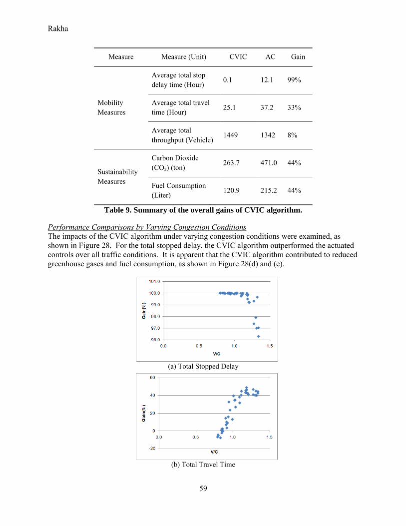
Rakha

59

Measure Measure (Unit) CVIC AC Gain

Mobility Measures

Average total stop delay time (Hour)

0.1 12.1 99%

Average total travel time (Hour)

25.1 37.2 33%

Average total throughput (Vehicle)

1449 1342 8%

Sustainability Measures

Carbon Dioxide (CO2) (ton)

263.7 471.0 44%

Fuel Consumption (Liter)

120.9 215.2 44%

Table 9. Summary of the overall gains of CVIC algorithm.

Performance Comparisons by Varying Congestion Conditions The impacts of the CVIC algorithm under varying congestion conditions were examined, as shown in Figure 28. For the total stopped delay, the CVIC algorithm outperformed the actuated controls over all traffic conditions. It is apparent that the CVIC algorithm contributed to reduced greenhouse gases and fuel consumption, as shown in Figure 28(d) and (e).

(a) Total Stopped Delay

(b) Total Travel Time

Rakha

60

(c) Total Throughputs

(d) CO2

(e) Fuel Consumption

Figure 28. Gain comparisons under varying v/c ratios.

Despite the promising benefits observed under oversaturated conditions, the total travel times and the total throughputs showed marginal improvements under uncongested conditions, i.e., v/c of 0.9 or less. To investigate such challenging performances, t-tests (α=0.05) used to statistically examine the difference of means between the two control methods were conducted. Figure 29 shows the p-values of total travel time (i.e., Figure 29(a)) and total throughputs (i.e., Figure 29(b)) under varying v/c ratios. As clearly shown in Figure 29(a), while the gains obtained from the CVIC algorithm are statistically significant when v/c ratios are 0.9 or higher, no gains were observed when v/c is less than 0.9. Total throughputs are similar to the cases of total travel time but its boundary v/c ratio was 1.0. Taking into consideration that the v/c ratio of each volume scenario was estimated by the optimized timing plans for the ACs, v/c ratios of less than 1.0 mean that the capacity of the intersection is adequate to treat the approaching demands. Thus, the total throughputs of ACs under such 1.0 v/c ratio cases would be similar to those of the CVIC algorithm, as clearly shown in Figure 29(b).

Rakha

61

(a) Total Travel Time

(b) Total Throughputs

Figure 29. T-test comparisons under varying v/c ratios.

Under uncongested conditions, i.e., v/c is 0.8 or less, cars maintain free-flow speeds, although they need to stop at the intersection if the intersection is operated by an AC. On the contrary, in the CVIC algorithm – the design of which compels vehicles to cross the intersection without waiting at the stop-bar – vehicles are manipulated to maintain the optimal speeds to cross the intersection. However, when the optimal speeds are below the free-flow speeds, the travel times of CVIC vehicles are longer than those of the ACs, particularly when traffic conditions are uncongested; Figure 29 (a) proves such an interpretation. However, it is noted that the travel times under uncongested conditions could be improved by adjusting the control parameters (such as the minimum speed, the maximum deceleration rate, or the minimum time headways) fed by fixed values for the simulation experiments in this section.

2.4 Conclusions and Recommendations Through a simulation test bed developed for this research, the potential improvements of the CVIC algorithms were evaluated under varying traffic congestion conditions. Results showed that the CVIC algorithm outperforms conventional actuated control systems in both mobility and sustainability.

The CVIC algorithm significantly improved the stopped delay at the intersection compared to the AC. The stopped delay was reduced by 99%, and the total travel times and total throughputs were also improved by 33% and 8%, respectively. In addition to such improvements for the

Rakha

62

mobility of an intersection, the CVIC algorithm significantly improved air quality and energy savings with a 44% reduction in CO2 gases, and 44% savings in fuel consumption.

In particular, it was observed that the CVIC algorithm outperformed the AC when an intersection was being operated under oversaturated conditions. While the travel time savings were approximately 18% at most under moderate congestion conditions (i.e., v/c ratio of 1.0 or less), about 60% of travel time reduction was observed when the v/c ratio was 1.0 or more. This observation indicates that the CVIC algorithm increases the capacity of the intersection by reducing the delay time at the intersection, as indicated by the approximately 23% increase of total throughput.

The boundary values of the CVIC algorithm constraints presented in Table 9 were specified to fixed values for the entire traffic congestion conditions in this research. However, such boundary values would vary with the congestion conditions; for instance, under lower congestion conditions, it would be acceptable to adjust the speed constraints to be higher as the risks of collisions are relatively lower than in higher congested conditions. Such optimally adjusted constraints would improve the performance of the proposed algorithm.

While the case study was demonstrated on a four-way isolated intersection with a single through-lane for each approach, the CVIC algorithm was developed for a generic intersection with multi-lanes and left-turn bays as shown in the objective function in Equation (24). In addition, the CVIC algorithm is expected to improve the operations of consecutive intersections on a corridor where their progressions are coordinated by predefined offsets among the intersections under both pre-timed and actuated controls. Although this research did not perform proper case studies for both multi-lane and coordinated intersections, the implementations for such case studies would be feasible as future research.

3. Cumulative Travel-time Responsive (CTR) Real-Time Intersection Control Algorithm under the VII Environment Recently, the VII initiative enabled the introduction of a mobile wireless communications technology into transportation safety, operations, and management (ITS, 2011). VII provides a two-way wireless communication environment enabling vehicle-to-vehicle (V2V) and vehicle-to-infrastructure (V2I) communications. Thus, vehicles equipped with communication devices and infrastructure within the VII environment could collect previously unobtainable and high fidelity traffic data, such as individual vehicles’ maneuvers, origins/destinations, and trajectories, and share such traffic information with other equipped vehicles and infrastructure. This previously unobtainable information from VII can contribute to intersection control by overcoming the challenges resulting from a lack of proper information for conducting the most efficient operations.

Current adaptive traffic control systems rely heavily on predictions to gain proper control strategies. The majority of such predictions are the anticipation of arrival patterns, turning designations, and approaching demands at downstream intersections. However, it is generally understood that prediction inaccuracy is blamed for inferior performance of the adaptive control. This is because the stochastic nature of vehicles’ movements would not be properly captured by the prediction models used in the adaptive control systems. Nevertheless, such predictions are utilized because existing sensing technologies, including inductive loops or video cameras, used

Rakha

63

in the current adaptive system are incapable of directly measuring individual vehicles’ driving information mentioned above. Given such individual vehicular information it would be unnecessary to keep the current prediction-based framework of the adaptive signal control systems. Thus, VII would benefit from designing a new adaptive control system that can fully utilize such sensing capability.

This study proposes a novel adaptive intersection control algorithm called CTR real-time control algorithm. The CTR algorithm employs individual vehicles’ cumulative travel time (CTT) directly measured (under 100% market penetration rate) or estimated (under imperfect market penetrations) from within the VII environment. Since the accuracy of information collected from VII depends on how many vehicles are equipped with the VII devices, the CTR algorithm adopted a Kalman Filter (KF)-based estimation technique to account for imperfect market penetration conditions. The main objectives of this research were to (i) quantify the potential benefits of the CTR algorithm under varying traffic conditions and VII market penetration rates, and (ii) determine a minimum market penetration rate that can benefit the CTR algorithm under VII.

3.1 Literature Review The CTR algorithm proposed in this study is an adaptive intersection control system designed to react to the travel time of individual vehicles. Details about the adaptive control systems in terms of vehicle arrival prediction were introduced in Chapter 1. Such control systems depend on projections of vehicle arrivals. However, it is noted that vehicle arrival predictions become somewhat unreliable when only fixed-point sensors are used. This is because the stochastic nature of vehicular movements makes the perfect predictions of vehicles’ arrivals almost impossible. Information quality, such as CTT accuracy, available from the VII environment is largely dependent upon market penetration rates. Unless every vehicle is equipped with a proper communication device, the accuracy of the collected information might not be sufficient to be properly used as the online measure of the CTR algorithm. The uncertainty introduced by this issue has been frequently addressed in the estimations of traffic states such as travel times, speeds, and queue length.

Numerous research efforts to address this limitation have been proposed. In particular, several researchers have applied the KF technique to improve estimation and have demonstrated its promising benefits.(Welch 2011) Ye et al. (Ye 2006) proposed a speed estimation method for single-loop detectors. While single loop detectors are adequate to count traffic volumes, estimating speeds with them is a known limitation, as the lengths of vehicles cannot be correctly accounted for. To address such a limitation, the authors proposed an unscented Kalman Filter (UKF) (Simon 2006) technique with a non-linear state-space equation. Compared to other speed estimation methods, UKF showed 70~40% and 63~28% of the mean absolute error (MAE) improvements against the g-estimator (Lin 2004) and the dynamic g-estimator(Wang 2000), respectively.

Guo et al. (Guo 2002) also proposed a single-loop speed estimation method based on the KF technique. Unlike Ye et al.(Ye 2006), their approach was based on a linear state-space equation derived from the relationship between flow-occupancy ratio and speed. With collected data from double-loop detectors located on eight different interstate highway sections in Northern Virginia (i.e., I-66) and Northern California (i.e., I-95), the authors estimated eight different regression

Rakha

64

models corresponding to the state-space models covering each of eight sections. Meanwhile, the measurement equations were calibrated with the flow-occupancy ratios and speeds as dependent and independent variables, respectively. In addition, with respect to the estimations of noise variances, they suggested that the use of residual errors obtained from the regression models would be appropriate to implement the KF algorithm. The proposed KF-based speed estimation method consistently outperformed the conventional g-factor method.

Jun et al. (Jun 2006) performed a comparison study for three different smoothing methods to reduce the random errors from the global positioning system (GPS). Those smoothing methods include: i) a least-square spline approximation, ii) a kernel-based smoothing method, and iii) a KF technique. The authors stated that given well-estimated state and measurement error variances, the KF technique would be the most suitable method to minimize the errors. With respect to the travel distance error, the KF-based method showed outstanding performance (e.g., 0.192 miles in MAE), whereas those errors from the least-square approximation and kernel-based methods appeared to be 9.79 and 5.71 miles, respectively.

In summary, the KF technique has outperformed various similar methods in dealing with either traffic state estimations or noise reductions. Such outstanding performance is the result of the feedback characteristic of the KF technique to recursively correct the errors within the boundary set by both process and measurements’ noise variances. Consequently, the reviews presented in this section provide evidence that the KF technique could be successfully utilized as the estimation method for CTT under imperfect VII market penetration rates.

3.2 Methodology 3.2.1 Cumulative Travel-time Responsive (CTR) Real-Time Intersection Control CTT as a Real-time Control Measure In general, travel time is defined as time spent by a vehicle to pass a certain roadway section. While the travel time measure has been used by traffic management centers to inform drivers on freeways or arterials, none of the adaptive traffic signal control systems have employed travel time as a real-time measure for determining traffic signal timing. The reasons why travel time has not been used for the measure are obvious: i) the travel time is calculated by vehicles that have completely passed the roadway section, and ii) the update interval of travel time estimation is relatively long (i.e., 5-minute). For instance, when a travel time section is defined from the upstream stop bar to the downstream stop bar and there are several vehicles waiting for the green phase near the downstream stop bar, the travel time of those waiting vehicles would be considered as zeros until the signal changes to green so that the queued vehicles completely leave the travel time collection section. Indeed, the update interval (e.g., 5 minutes) used in calculating travel time estimation is too long to react to rapidly changing intersection states.

Therefore, this study proposes a CTT, defined as the elapsed time spent by vehicles from the time they enter the approach link, as the real-time measure of the proposed intersection control algorithm. The CTT that is updated in a short time interval (e.g., 5 s) enables the proposed intersection control algorithm to rapidly react to the dynamic changes in traffic and to take into consideration the vehicles’ location at any point on an approach, thus preventing potential measurement distortions.

Rakha

65

Control Algorithm The CTR algorithm updates the CTT of every vehicle on the respective approach. Then, the algorithm aggregates the total CTT of possible NEMA phase combinations (e.g., phases 1&6, 2&5, etc.) and determines the highest CTT phase. If the selected phase is the same as the current green phase, then the current green time is extended to the duration of an update time interval. Otherwise, the current green phase is switched to the next green interval after the change interval (i.e., yellow and red clearance intervals).

For example, suppose that phases 2 and 6 were selected for the highest CTT phases at time t-1 followed by time t-2, as shown in Figure 30. Thus, the phases 2&6 are kept green, whereas the other phases are kept red. Then, at time t, the algorithm evaluated the CTT for the respective phases and determined phases 4&8 as the new green phases. Therefore, the old green phases are changed to yellow for a prespecified yellow interval, while the other phases stay red until the yellow interval. After the yellow, phases 4&8 are changed to green.

Figure 30. Conceptual control logic of proposed algorithm.

While the CTTs from the VII-device-equipped vehicles can be directly observed, the CTTs of all other vehicles (including non-equipped vehicles) would need to be estimated. This is because, under imperfect market penetration conditions, direct use of collected CTTs would undermine the overall performance of the CTR algorithm. To address this issue, this research employs a stochastic estimation method based on the KF technique. As noted in the literature review, the KF technique has proven to be effective.

3.2.2 Standard Kalman Filter Algorithm The KF is comprised of two equations: i) a state-space equation and ii) a measurement equation. The

state-space equation affirms that the current states, denoted as , are resulting from i) the previous states, denoted as , ii) the previous input actions, , and iii) noises which occurred at the previous time period. The measurement equation explains that the current measurements, denoted as , can be obtained from the current estimated states, or vice versa with some noise.

Rakha

66

(29)

(30)

where,

x: State vector (n × 1); A: State mapping matrix (n × n); u: Input variable vector (1 × m); B: Input mapping matrix (m × n); w: State random variable ( ~ 0, ); z : Measurement vector (n × 1) ; H: Measurement mapping matrix (n × n) Q: State noise covariance; v: Measurement random variable ( ~ 0, ); R: Measurement noise covariance; and k : Time interval index

The KF uses a recursive estimation procedure: it repeats i) state estimations and ii) state corrections. The SKF algorithm deploys this recursive process by decomposing both state-space and measurement equations which have linear forms.(Welch 2011)

3.2.3 Derivations of Equations In order to accurately estimate CTTs, this study assumed that the total vehicle counts on a certain roadway, or a left-turn bay, would be obtained at every certain time interval from existing sensing technologies, such as traffic monitoring cameras or inductive loop detectors. Taking into consideration the evolution of vehicle sensing technologies that have been deployed in the field, this assumption would be acceptable. With the known total vehicle counts, an equipped vehicle ratio can be determined and used as a state correction factor for the measurement equation.

State-space Equation Derivation The basic form of a state-space equation is already shown in Equation (29). The equation must have the current state vector, the previous state vector, and the state-transition matrix, denoted as xk, xk-1, and A, respectively. The input action matrix (u) and its transition matrix (B) are optional based on the characteristics of a dynamic system. Those two matrices are utilized to account for the relationship between control activities and the results.

At an intersection, the current state, referred to as the CTT, would be affected by various external factors (or input activities) such as the number of vehicles approaching the intersection, signal status (i.e., green or red), and geometrical characteristics (e.g., number of lanes, length, or existence of left-turn bay). Obviously, in order for the state-space equation to be as accurate as possible, these factors should be properly taken into account. As such, this paper performed preliminary statistical analysis to see which equation form yields the most representative state-space equations as in Equation (31-33), and Equation (31) was selected for the final form. Note that the coefficients for the travel times (denoted as , , and ) and for the traffic counts (denoted as and ) in Equation (31) indicate the

Rakha

67

components of the state mapping matrix A, and the input mapping matrix B, respectively, in Equation (29).

, , , , 2,4,6,8

, , , , 1,3,5,7 (31)

, , , , , 2,4,6,8

, , , , , 1,3,5,7 (32)

, , , , , 2,4,6,8

, , , , , 1,3,5,7 (33)

where,

α : Cumulative travel time coefficient for through traffic β : Total count coefficient for through traffic γ : Cumulative travel time coefficient for left-turn traffic δ : Corresponding through traffic cumulative travel time coefficient for left-turn

traffic ε : Total count coefficient for left-turn traffic μ : Green time coefficient for through traffic τ : Green time coefficient for left-turn traffic σ : Coefficient of total number of lanes for through traffic i : Phase number index j : Corresponding through traffic phase number index for left-turn traffic t , : Total cumulative travel time of phase i at time interval k q , : Total number of vehicles of phase i at time interval k g , : The amount of green time in seconds of phase i at time interval k

: Total number of lanes of phase i The subscripts i and k in Equation (31-33) indicate the signal phase number based on the

NEMA standard, and the time interval, respectively. The subscript j denotes the corresponding through-traffic NEMA phase number given i (i.e., (i,j) = (1,6), (5,2), (3,8), and (7,4)). Accordingly, Equation (31) indicates that i) the current CTTs of through phases (e.g., i = 2,4,6,8) are influenced by the previous CTTs and the total number of vehicles at the beginning of the current time period, and ii) the current CTT of left-turn phases (e.g., i = 1,3,5,7) are affected by the previous CTT of left-turn phase, total number of vehicles on the left-lane bay, and the previous CTT of corresponding through phases. It is noted that the CTR algorithm considers the left turn lane as an independent approach and applies the same estimation process used in the through lane(s). When the length of the left turn bay is shorter than the through lanes, CTTs of vehicles making left turns would be influenced by through traffic before they enter the left turn bay. Thus, the state-space equation of left-turn

Rakha

68

phases considers the previous CTT of the through traffic. The vector and matrix formations of a state-space equation for a four-legged intersection, shown in Figure 31, are written in Equation (34).

Figure 31. NEMA phase numbering scheme for an intersection.

+ (34)

where,

: State vector for the cumulative travel time at time interval k (equivalent to xk in Equation (30))

( , , , , , , , , , , , , , , ,

: Vector for the total traffic counts at time interval k (equivalent to uk in Equation (30)

, , , , , , , , , , , , , , ,

A: State-space transition matrix

0 0 0 0 0 00 0 0 0 0 0 00 0 0 0 0 00 0 0 0 0 0 00 0 0 0 0 00 0 0 0 0 0 00 0 0 0 0 00 0 0 0 0 0 0

Rakha

69

B: Input transition matrix

0 0 0 0 0 0 00 0 0 0 0 0 00 0 0 0 0 0 00 0 0 0 0 0 00 0 0 0 0 0 00 0 0 0 0 0 00 0 0 0 0 0 00 0 0 0 0 0 0

, , : State-space equation coefficients. See Equations (31-33). , : Control equation coefficients. See Equations (31-33).

Measurement Equation Derivation The measurement equation adjusts estimated states with actual measurements. In other words, the gap between the measured states obtained from communication-device-equipped vehicles and the estimated states obtained from the state-space equation is adjusted by the measurement transition matrix, H, as was shown in Equation (30). Notice that the measurement transition matrix would be an identity matrix (i.e., I) if all vehicles have communication devices.

, , / , (35)

, , , , (36)

where,

: Measurement transition coefficient , : The ratio of equipped vehicles ( , ) over the total number of vehicles ( , ) for phase i at time interval k

With the total number of vehicles and the number of equipped vehicles on a certain intersection approach, i, at time k, an equipped vehicle ratio can be defined in Equation (35). Since measured CTTs, denoted as , , are known to be actual CTTs during the estimation process, in Equation (36) was obtained as the

measurement transition coefficient to approximate the measured CTTs to actual CTTs. Therefore, the final measurement equation for a four-legged intersection as shown in Figure 31 is established as Equation (37):

(37)

where,

: Adjusted CTT vector at time period k

, , , , , , , , , , , , , , ,

: Measured CTT vector at time interval k

, , , , , , , , , , , , , , ,

H: Measurement transition matrix

Rakha

70

0 0 0 0 0 0 00 0 0 0 0 0 00 0 0 0 0 00 0 0 0 0 0 00 0 0 0 0 0 00 0 0 0 0 0 00 0 0 0 0 0 00 0 0 0 0 0 0

Determination of Noise Covariance Matrices In general, the noise covariance matrices for the state-space equation and the measurement equation, denoted as Q and R in Equations (29) and (30), respectively, are known to be difficult to determine (Elango 2000). Typically, these two matrices are obtained through an off-line tuning process based on a trial-and-error approach in practical SKF applications.

To overcome this issue, the use of Adaptive Kalman Filter (AKF) has been proposed by a few researchers in the transportation field (Chu et al., 2005). The basic idea of AKFs is to update the covariance matrices at every time interval by using covariance matching techniques such as multiple model adaptive estimation (MMAE) and innovation-based adaptive estimation (IAE) (Mohamed 1999). While AKF algorithms would be more appropriate than SKF, such techniques require additional computation efforts to implement, often preventing rapid implementations. Moreover, at times, the size of residual samples, determined by the estimation of covariance matrices in the IAE technique, would affect the propagation of such matrices (e.g., if the sizes are too small, the matrices would be propagated too randomly), likely resulting in inaccurate state estimations (Mohamed 1999).

To avoid such inaccuracies, an off-line tuning approach based on the residual errors of the estimated regression models was employed. To this end, the variances of the three equations, i.e., state-space equations for: i) through, ii) left-turns, and iii) measurement equations, were estimated on the basis of the regression models (Guo 2002).

3.2.4 Estimations of the State-Space Equations and the Measurement Equations This study adopted a regression-based model as proposed by (Guo 2002) to estimate the matrices in Equations (29) and (30). The research team first tried to estimate coefficients’ matrices by utlizing vehicles’ actual trajectories recorded in the Next Generation Simulation (NGSIM) data set (http://ngsim-community.org). Although the NGSIM data provide detailed vehicular trajectories traveling on actual corridors, they did not have sufficient data to develop a generalized model. This is because data were available from only a few selected roadway sections. Due to such limitations in observed data from the NGSIM data set, this paper utilized simulation-based experiments, designed by the LHD approach (McKay 2000), to obtain individual vehicular data from general traffic situations.

Building the Hypothetical Data Set with LHD Figure 32 depicts a base intersection used for the simulation experiments. The intersection has four approaches and each of them has a single left-turn lane and varying numbers of through lanes. The lengths of each approach and left-turn bay are also created by the LHD. The input volumes for each approach and left-turn to through traffic ratios were also designed by the LHD. A total of 50 scenarios were created by the LHD, and the experimental factors and the levels

Rakha

71

used in the scenario developments are summarized in Table 10. The traffic signal timing plan for each scenario was optimized by the TRANSYT-7F program (Hale 2005) with an assumption that the intersection is operated under an actuated signal control system.

Figure 32. Screenshot of base experimental network.

Factors Levels

Input Volumes per lane for each Approach (vph) 300~1700

Turning Movement Ratio (Left-Turn/Through) 0.1~0.4

Link Length (ft) 150~1000

Left-Turn Bay Length Ratio (Left-Turn/Through) 0.2~0.7

Table 10. Factors and levels for simulation experiments.

Model Estimations The coefficients in Equations (31-33) and (36) were estimated by regression models using SAS 9.0.(Peng 2009) Of the approximately 66,000 data records obtained from the experiments presented in the previous section, two different sub-data sets were randomly selected from the data record (e.g., Data Set-1 and Data Set-2) for the cross-validation of the regression models. Table 11 summarizes the estimation results based on Data Set-1 and Data Set-2.

Rakha

72

Equations Parameter

Data Set-1 Data Set-2 Coefficient T(p) Coefficient T(p)

State-space Equation for

Through Traffic

0.936 396.3(0.000) 0.938 403.1(0.000) 1.110 8.7(0.000) 1.100 8.3(0.000)

R2 0.97 0.96 N 3,293 3,294

State-space Equation for

Left-Turn Traffic

0.982 494.28(0.000) 0.965 445.66(0.000) -0.005 -6.10(0.000) -0.005 -6.68(0.000) 1.96 13.19(0.000) 2.610 17.57(0.000)

R2 0.99 0.99 N 3,293 3,294

Measurement Equation

1.003 1791.0(0.000) 0.999 1709.9(0.000)R2 0.99 0.99 N 4,872 4,872

Table 11. Coefficients estimated from the simulation experiments.

As shown in Table 11, the coefficients estimated from both data sets are almost identical, and the coefficients of determinations, R2s, are close to 1.0. Knowing that the two data sets were obtained from randomly selected sample data sets, the estimated models from either Data Set-1 or Data Set-2 would be considered reliable. The coefficients obtained from Data Set-1 were selected to be used for the state-space and measurement equations as given in Equations (38) and (39), respectively.

+ (38)

(39)

where,

A =

0.982 0 0 0 0 0.005 0 00 0.936 0 0 0 0 0 00 0 0.982 0 0 0 0 0.0050 0 0 0.936 0 0 0 00 0.982 0 0 0.005 0 0 00 0 0 0 0 0.936 0 00 0 0 0.005 0 0 0.982 00 0 0 0 0 0 0 0.936

B=

1.96 0 0 0 0 0 0 00 1.11 0 0 0 0 0 00 0 1.96 0 0 0 0 00 0 0 1.11 0 0 0 00 0 0 0 1.96 0 0 00 0 0 0 0 1.11 0 00 0 0 0 0 0 1.96 00 0 0 0 0 0 0 1.11

Rakha

73

H=1.003

0 0 0 0 0 0 00 0 0 0 0 0 00 0 0 0 0 0 00 0 0 0 0 0 00 0 0 0 0 0 00 0 0 0 0 0 00 0 0 0 0 0 00 0 0 0 0 0 0

To validate the coefficients, the performances of coefficients estimated for the equations in KF models were examined through a randomly generated simulation data set. To this end, a Root Mean Square Error (RMSE) and a Mean Absolute Percentage Error (MAPE), shown in Equations (40) and (41), respectively, were used. As a result, about 20% of MAPE for state-space equations were assessed while that of the measurement equation was approximately 9%, as summarized in Table 12.

RMSE∑

(40)

MAPE ∑ (41)

where,

: actual travel time : estimated travel time by the equations : Total data counts

RMSE MAPE (%) State-space Equations

Through 36.0 20.5 Left-turn 17.9 20.5

Measurement Equation 13.6 8.9 Table 12. Performance of estimated equations obtained from simulation experiments.

3.3 Evaluations 3.3.1 Assumptions The CTR algorithm is based on a discrete time-dynamic system that requires state updates at every certain time interval. Therefore, the update interval would be another crucial factor for the system’s performance, but finding the best update interval would also add extra computational burdens for this research. As such, based on several preliminary efforts to investigate the proper updated interval, an update interval of 5 s for the simulation of the CTR algorithm was determined.

Rakha

74

3.3.2 Simulation Test Bed The simulation test bed that incorporated the simulations of the VII environment and the implementation of the KF algorithm was developed with VISSIM and the VISSIM COM (Planung Transport Verkehr 2009; Planung Transport Verkehr 2009) interface. For efficient matrix manipulations required for the online implementations of the KF algorithm, it was compiled as a stand-alone Dynamic Linked Library (DLL) in MATLAB . (Mathworks 2009)

As depicted in Figure 33, VISSIM collects travel time measurements at every update interval, and sends them to the KF module through a communication channel provided by VISSIM’s COM interface. The KF module performs the KF algorithm, including matrix manipulations, and sends the estimated traffic states back to the VISSIM through the COM interface. Based on the estimated traffic states, the traffic signal control module developed under the COM interface determines the optimal green phases and implements the corresponding signal operations. This recursive task was implemented repeatedly until the simulation ended.

Figure 33. Conceptual architecture of the simulation test bed.

3.3.3 Measures of Effectiveness (MOEs) To evaluate the performance of the proposed CTR algorithm, two types of MOEs were selected: i) mobility measures, and ii) sustainability measures. The mobility measures selected in this study were: i) total travel time, ii) average speed, and iii) maximum throughputs. To investigate the sustainability impacts of the proposed algorithm, a microscopic emissions and fuel consumption estimation model, called the VT-Micro Model (Ahn 2002), was employed. The VT-Micro model estimates the amount of CO2 and fuel consumption based on instantaneous speed and acceleration data. All MOEs with respective units used are summarized in Table 13.

MOE Category MOE Unit

Mobility Measure Total Travel Time Vehicle-Hour

Average Speed KPH Maximum Throughput Vehicles

Sustainability Measure Carbon Dioxide (CO2) Ton

Fuel Consumption Liter

Rakha

75

Table 13. Summary of MOEs.

3.3.4 Evaluation Scenarios A hypothetical isolated intersection, as shown in Figure 34, was used for the evaluations. The intersection has four approaches and each approach has two through lanes and a single left-turn bay.

Figure 34. A hypothetical isolated intersection in VISSIM simulation.

Evaluation scenarios were designed with two major experimental factors: i) intersection volumes, and ii) market penetration rates. With the consideration of required computation running time, a total of 40 volume scenarios covering the volume capacity ratio ranging from 0.3 to 1.1 were generated by LHD. The market penetration rates were uniformly divided into six levels: 10%, 30%, 50%, 70%, 90%, and 100%. A total of 7,200 evaluation scenarios were developed and 30 replications were made for each scenario. For comparison purposes, the actuated traffic signal timing plan for each volume scenario was developed using the TRANSYT-7F program.(Hale 2005)

3.4 Results 3.4.1 Overall Performances under 100% Market Penetration The performance of the CTR algorithm was evaluated at 100% market penetration rate. When compared to the actuated control (AC, as summarized in Table 14, the CTR algorithm significantly improved the mobility measures such as travel time and average speed, resulting in 34% and 36% improvement, respectively. The total number of vehicles that passed through the intersection was also improved by 4% with the CTR algorithm. In addition, the greenhouse gases and fuel consumption were also improved by 13% and 10%, respectively.

Rakha

76

Measure AC CTR (100%)

Gain (%)

p-value

Total travel time (h) 27.9 18.4 34 0.000Speed (kph) 32.5 44.3 36 0.000

Throughput (vehicle) 1294.5 1343.8 4 0.036CO2 (ton) 350.7 306.9 13 0.000

Fuel Consumption (liter) 165.1 148.1 10 0.000

Table 14. Overall performances of CTR algorithm (100% market penetration).

3.4.2 Impacts of Imperfect Market Penetrations The overall savings under varying market penetration rates are summarized in Figure 35. The total travel time, average speed, and total throughputs are denoted as VHT, SPD, and THR, respectively, in Figure 35. It shows that when the market penetration rates exceed 30%, the CTR algorithm would produce greater benefits as compared to the actuated controls. In addition, the greenhouse gases and fuel consumption showed significant benefits throughout the entire market penetration rates, as shown in Figure 35. However, those benefits become smaller as the market penetration rates increase. In summary, the simulation results showed that mobility benefits can be achieved when the market penetration rate exceeds 30%. In the next section, the impacts of congestion levels are presented.

Rakha

77

Figure 35. Change of savings under different market penetration rates.

3.4.3 Impacts of Congestion Levels Even with the same market penetration rates, the performance of the proposed CTR algorithm varies based on the level of congestion. In Figure 36, the total travel time savings under varying intersection volumes tend to increase as: i) the market penetration rates increase, and ii) the total intersection volumes increase.

The 10% market penetration rate cases did not result in any significant savings for almost all volume cases compared to the actuated control, as shown in Figure 36. However, with the 30% market penetration rate, positive mobility benefits were observed when the total volumes were 3,000 vph or more. It is noted that the 3,000 vph represents the v/c ratios between 0.6 and 0.8, and Level of Service (LOS) C or, occasionally, D. In other words, when the market penetration rate reaches 30%, the CTR algorithm improves the mobility of an intersection if it is being

Rakha

78

operated at LOS C or D under the actuated signal control. The mobility benefits appeared to increase as the market penetration rates increased. At the 70% market penetration rate, the proposed CTR algorithm outperformed the actuated controls over entire volume cases.

Figure 36. Improvements for mobility (left) and sustainability (right) measures by volume

cases.

For the sustainability measures, their trends compared to those of the volume levels are of interest. As demonstrated in Figure 36(d) and (e), in most cases the CTR algorithm outperformed the actuated controls except for several low volume cases at 100% market penetration rates. As shown in Figure 36, the reductions of CO2 and fuel consumption were gradually decreased as the market penetration rates increased. This is likely attributable to increase in speed.

Rakha

79

3.5 Conclusions and Recommendations In this study, a CTR real-time intersection control algorithm under VII was developed and its performance was evaluated under varying market penetration rates. The proposed algorithm utilized individual vehicular travel time on the approach of an intersection – namely the CTT – within the VII environment. The performance of the proposed algorithm was evaluated through a simulation-based test bed under varying traffic congestion levels and market penetration rates.

At the 100% market penetration rate, the CTR algorithm significantly improved the mobility of an intersection when compared to the actuated controls. For example, the total travel times were decreased by 34% and the average speeds increased by 36%. As a result, the throughput of the intersection also increased by 4%. Furthermore, the proposed algorithm contributed to a reduction in the amount of greenhouse gases and fuel consumption, resulting in 13% reductions in CO2 and fuel savings of 10%.

As expected, the performance of the CTR algorithm was affected by the market penetrations of the VII vehicles. Lower market penetration rates (i.e., 30% or less) degraded the performance of an intersection’s mobility. This is due to the insufficient accuracy of the estimated CTT resulting from the imperfect market penetration rates. On the other hand, it was observed that the intersection’s mobility improved as long as the market penetration rates exceeded 30%; the mobility measures such as total travel times, average speeds, and total throughputs linearly improved as the market penetration rates increased. However, the improvements of the sustainability measures such as CO2 and fuel consumption were linearly decreased as the market penetration rates increased.

The impact of traffic congestion on the CTR algorithm performance was also examined. At the 30% market penetration rate, improvements were observed when the total volumes exceed 3,000 vph, equivalent to v/c ratios of 0.6~0.8. This observation indicates that the CTR algorithm would be beneficial for intersections that are being operated at LOS C or D as long as market penetration rates exceed 30%.

In this research, the CTR algorithm was developed and evaluated through a hypothetical isolated intersection-based case study. It is likely that the CTR algorithm can be successfully applied to coordinated intersections by assigning weighting factors to the vehicles on the major streets, as demonstrated by Porche and Lafortune.(Porche and Lafortune 1999)

Although the CTR algorithm was developed to pursue an adaptive traffic control system, its performance was compared to the actuated control system in this study. This is because the research team was unable to obtain adaptive control programs that can be implemented in microscopic traffic simulators like VISSIM or CORSIM. It is noted that several adaptive programs exist but they are not opened to public as of yet. Thus, the performance of the CTR algorithm should be examined through a comparison study with the adaptive control systems should they become available for use in the future.

As previously mentioned, it was discovered that 30% of the VII market penetration rate is the marginal rate that can show the benefits of the CTR algorithm. According to a recent investigation on VII deployments, 50% of market share will be reached in the next

Rakha

80

decade.(Partner 2009) Thus, the performance of the CTR algorithm to the real world can be examined in the near future.

Rakha

81

PART IV: CONCLUSIONS VII links vehicles, drivers, and the surrounding infrastructure (which includes roadways, traffic controls, etc.). It can bridge the infrastructure and individual drivers and, therefore, improve the efficiency of traffic systems and promote transportation safety. In this research, the feasibility and benefits of three advanced intersection control systems are investigated. All three systems exhibit significant improvements in reducing travel time and stop delays, as well as pollution. The first system reduced the total intersection delay by 65%. The second system reduced stopped delays by 99% and total travel time delays by 33%; it also decreased CO2 gases by 44%. The total throughputs are improved by 8%. The third showed comparable reductions in delay and tailpipe emissions. Market penetration is proved to be influential on the performance of such systems. It was observed that the intersection’s mobility improvement is significant as long as the market penetration rates exceeded a marginal percentile of 30 percent.

VII provides a bright future in the development of next generation intersection control systems. The results from this research testify that an efficient utilization of advanced technology of detection and communication as well as the high quality data acquired by such technology will benefit the efficiency of transportation systems. Delays and the associated environment problems at intersections can be significantly reduced. Future work is needed to collect in-field data to further testify to the validity of such systems and more accurately measure the benefits.

Rakha

82

REFERENCES A. Boukerche, R. B. M., K.R.L. Juca, J.B.M. Sobral, and M.S.M.A. Notare (2007). "An agent based and biologically

inspired real-time intrusion detection and security model for computer network operations." Computer Communications 30: 2649–2660.

AASHTO (1954). A Policy on Geometric Design of Rural Highways. Washington, DC. Ahn, K., Rakha, H., Trani, A., Van Aerde, M. (2002). "Estimating Vehicle Fuel Consumption and Emissions based

on Instantaneous Speed and Acceleration Levels." Journal of Transportation Engineering 128(2): 182-190. Alonso-Ayuso, A., Escudero L. F., Martín-Campo, F. J. (2010). "Collision Avoidance in Air Traffic Management: A

Mixed-Integer Linear Optimization Approach." IEEE Transactions on Intelligent Transportation Systems 12(1): 47-57.

Andrews, C. M., S. M. Elahi (1997). Evaluation of New Jersey Route 18 OPAC/MIST Traffic Control System. 76th Annual Meeting of the Transportation Research Board, Washington, DC.

B.Greenshields, D. S., E.Ericksen (1947). Traffic Performance at Urban Street Intersections. Yale Bureau Of Highway Traffic.

Banks, J. H. (1991). "Two-capacity phenomenon at freeway bottlenecks : a basis for ramp metering?" Transportation research record.(1320): p. 83-90.

Bazzan, A. L. C. (2005). "A Distributed Approach for Coordination of Traffic Signal Agents." Autonomous Agents and Multi-Agent Systems 10(1): 131-164.

Board, T. R. (2000). Highway Capacity Manual 2000. Transportation Research Board. Brian, W., Arthur, S. N. Durlauf, D. Lane (1995). The Economy as an Evolving Complex System II, SFI Studies in

the Sciences of Complexity. Global Economy Workshop, Santa Fe, New Mexico, Addison Wesley. Bullock, D., T. Urbanik (2000). Traffic Signal Systems: Addressing Diverse Technologies and Complex User Needs.

Transportation in the New Millennium. Washington DC, National Research Council. Bullock, D. and T. Urbanik (2000). Traffic Signal Systems: Addressing Diverse Technologies and Complex User

Needs. Transportation in the New Millennium. Washington DC, National Research Council. Caliendo, C., Guida, M., Parisi, A. (2007). "A crash-prediction models for multilane roads." Accident Analysis and

Prevention 39(4): 657-670. Caudill, R. J., Youngblood, J.N. (1976). "Intersection merge control in automated transportation systems."

Transportation Research Part B: Methodological 10(1): 17-24. Charania, A. C., J.R. Olds, D.DePasquale (2006). Sub-Orbital Space Tourism: Predictions of the Future Marketplace

Using Agent-Based Modeling. 57th International Astronautical Congress, Valencia, Spain, SpaceWorks Engineering, Inc.

Chaudhary, N., V. Kovvali, C. Chu, S. Alam (2002). Software for Timing Signalized Arterials. College Station, Texas, Texas Transportation Institute, The Texas A&M University System.

Chen, B., Harry H. Cheng (2010). "A Review of the Applications of Agent Technology in Traffic and Transportation Systems." IEEE Transactions on Intelligent Transportation Systems 11: 485-497.

Chen, C.-Y. (2005). "California Intersection Decision Support: A Systems Approach to Achieve Nationally Interoperable Solutions." California PATH Research Report UCB-ITS-PRR-2005-11.

Chung, K., J. Rudjanakanoknad, et al. (2007). "Relation between traffic density and capacity drop at three freeway bottlenecks." Transportation Research Part B: Methodological 41(1): 82-95.

Cohen, S. L. (2002). "Application of car-following systems to queue discharge problem at signalized intersections." Transportation Research Record(1802): 205-213.

Daganzo, C. F. and R. C. Garcia (2000). "Pareto improving strategy for the time-dependent morning commute problem." Transportation Science 34(3): 303-311.

Dia, H. (2000). A conceptual framework for modelling dynamic driver behaviour using intelligent agents. the 6th International Conference on Applications of Advanced Technologies in Transportation Engineering. Singapore: 28-30.

Dia, H. (2002). "An agent-based approach to modelling driver route choice behaviour under the influence of real-time information." Transportation Research Part C 331-349.

Dia, H. and H. Purchase (1999). Modelling the impacts of advanced traveller information systems using intelligent agents. Road and Transport Research 8 (3), ARRB Transport Research Ltd. Vermont South, Victoria, Australia.

Douglas A. Reece, S. S. (1991). A computational model of driving for autonomous vehicles. C. M. U. Technical Report CMU-CS-91-122. Pittsburgh, Pennsylvania, USA.

Rakha

83

Dresner, K. and P. Stone (2004). Multiagent traffic management: A protocol for defining intersection control policies. Technical Report UT-AI-TR-04-315, The University of Texas at Austin, Department of Computer Sciences, AI Laboratory.

Dresner, K. and P. Stone (2004). Multiagent traffic management: A reservation-based intersection control mechanism. The Third International Joint Conference on Autonomous Agents and Multiagent Systems. New York, New York, USA: 530-537.

Dresner, K. and P. Stone (2005). Multiagent Traffic Management: An Improved Intersection Control Mechanism. The Fourth International Joint Conference on Autonomous Agents and Multiagent Systems. Utrecht, The Netherlands: 471-477.

Dresner, K. and P. Stone (2005). Multiagent Traffic Management: Opportunities for Multiagent Learning. K. Tuyls, et al, editors, LAMAS, Lecture Notes In Artificial Intelligence. Springer Verlag, Berlin.

Dresner, K. and P. Stone (2008). "A multiagent approach to autonomous intersection management." J. Artif. Int. Res. 31(1): 591-656.

Dresner, K., Stone, P. (2008). "A multiagent approach to autonomous intersection management." Journal of Artificial Intelligent Research 31: 591-656.

Econolite Control Products, I. (1996). ASC/2M-1000 Zone Master Programming Manual. Anaheim, California. Ehlert, P. A. M., L.J.M. Rothkrantz (2001). Microscopic traffic simulation with reactive driving agents. IEEE

Intelligent Transportation Systems Conference Proceedings. Oakland (CA) USA. Elango, C. a. D., D. (2000). "Irregularly Sampled Transit Vehicles Used as Traffic Sensors. ." Transportation

Research Record: 1719(33-44). Emonet, T., Macal, Charles, North, Michael, Wickersham, Charles, Cluzel, Philippe (2005). "AgentCell: a digital

single-cell assay for bacterial chemotaxis." Bioinformatics 21(11): 2714-2721. Garbacz, R. M. (2003). Adaptive Signal Control: What to Expect. Compendium of Papers of the ITE Annual

Meeting and Exhibit, Washington, DC, Institute of Transportation Engineers. Gartner, N. H., Chronis Stamatiadis, Phillip J. Tarnoff (1995). "Development of Advanced Traffic Signal Control

Strategies for Intelligent Transportation Systems: Mulitlevel Design." Transportation Research Record 1494: 98-105.

Glaser, S., Vanholme, B., Mammar, S., Gruyer, D., and Nouvelière, L. (2010). "Maneuver-Based Trajectory Planning for Highly Autonomous Vehicles on Real Road With Traffic and Driver Interaction." IEEE Transactions on Intelligent Transportation Systems 11(3): 589-606.

Goldberg, D. (1989). Genetic Algorithms in Search, Optimization, and Machine Learning, Addison-Wesley Professional.

Guo, J., Xia, J., Smith, B.L. (2002). "Kalman Filter Approach to Speed Estimation Using Single Loop Detector Measurements under Congested Conditions." Journal of Transportation Engineering 135(12): 927-934.

Hale, D., Uniersity of Florida (2005). Traffic Network Study Tool – TRANSYT-7F. United States Version. Gainesville, Florida, McTrans Center in the University of Florida.

Hall, F. L. and K. Agyemang-Duah (1991). "Freeway capacity drop and the definition of capacity." Transportation research record.(1320).

Hall, F. L. and L. M. Hall (1990). "Capacity and speed-flow analysis of the Queen Elizabeth Way in Ontario." Transportation research record.(1287).

Hamed, M., S. Easa (1997). "Disaggregate Gap-Acceptance Model for Unsignalized T-Intersections." Journal of Transportation Engineering 123(1): 36-42.

Head, K. L., P.B. Mirchandani, D. Sheppard (1992). "Hierarchical Real-Time Traffic Control." Transportation Research Record, Transportation Research Board, National Research Council, Washington DC 1360.

Henry, J., J.L. Farges, Tuffal, J. (1983). The PRODYN Real Time Traffic Algorithm. IFAC Control in Transport Systems, Baden-Baden, Federal Republic of Germany.

Hernandez, J., J. Cuena, et al. (1999). Real-time traffic management through knowledge-based models: the TRYS approach. Tutorial on Intelligent Traffic Management Models. Proceedings of the 11th Mini-Euro Conference on Artificial Intelligence in Transportation Systems and Science. Helsinki University of Technology, Espoo, Finland.

Hunt, P. B., D.I. Robertson, R.D. Bretherton, R.I. Winton (1981). SCOOT- A Traffic Method of Coordinating Signals. Crowthorne, Bershire, England, Transportation and Road Research.

Husch, D. A. a. A., Trafficwave, Inc. (2004). SYNCHRO 6 User Guide. IEEE (2006). IEEE Trial-Use Standard for Wireless Access in Vehicular Environments (WAVE) - Multi-Channel

Operation. IEEE Std 1609.4-2006: p. c1-74.

Rakha

84

ITS. (2011). "Connected Vehicle Research program (IntelliDrive)." Retrieved 2011, from http://www.its.dot.gov/connected_vehicle/connected_vehicle.htm.

J2735, S. (2009). Dedicated Short Range Communications (DSRC) Message Set Dictiona. Jakubiak, J. a. K., Y. (2008). State of the Art and Research Challenges for VANETs in Consumer Communications

and Networking Conference. 5th Annual IEEE Comsumer Communications and Networking Conference, Las Vegas, Nevada.

Jin, X., M. Itmi, et al. (2007). A cooperative multi-agent system simulation model for urban traffic intelligent control. Proceedings of the 2007 Summer Computer Simulation Conference, Society for Computer Simulation International, . San Diego, CA: 953-958.

Jun, J., Guensler, R., and Ogle, J. (2006). "Smoothing methods to minimize impact of global positioning system random error on travel distance, speed, and acceleration profile estimates." Transportation Research Record 1972: 141-150.

Kerner, B. S. (2008). "On-ramp metering based on three-phase traffic theory downstream off-ramp and upstream on-ramp bottlenecks." Transportation Research Record(2088): 80-89.

Kerner, B. S. and S. L. Klenov (2006). "Probabilistic breakdown phenomenon at on-ramp bottlenecks in three-phase traffic theory." Transportation Research Record(1965): 70-78.

Lin, F.-B. and D. R. Thomas (2005). "Headway compression during queue discharge at signalized intersections." Transportation Research Record(1920): 81-85.

Lin, W.-H., J. Dahlgren, H. Huo (2004). "Enhancement of Vehicle Speed Estimation with Single Loop Detectors." Transportation Research Record 1870: 147-152.

Lowrie, P. R. (1992). SCATS - Sydney Coordinated Adaptive Traffic System - A Traffic Responsive Method of Controlling Urban Traffic. Sydney Australia, Roads and Traffic Authority.

M. Van Aerde & Associates, Ltd. (2005). INTEGRATION Release 2.30 for Windows: User's Guide - Volume I: Fundamental Model Features.

M. Van Aerde & Associates, Ltd. (2005). INTEGRATION Release 2.30 for Windows: User's Guide - Volume II: Advanced Model Features.

Mannering, F. L. and W. P. Kilareski (1998). Principles of Highway Engineering and Traffic Analysis, John Wiley & Sons.

Mason, J. M., Fitzpatrick, K., Hardwood, D.W. (1990). "Field observations of truck operational characteristics related to intersection sight distance." Transp. Res. Record 1280, Transportation Research Board, Washington, D.C.: 163-172.

Mathworks, I. (2009). MATLAB&SIMULINK. McGinley, F. J. (1975). "An intersection control strategy for a short-headway P.R.T. network." Transportation

Planning and Technology 3(1): 45-53. McKay, M. D., Beckman, R.J., Conover, W.J. (2000). "A Comparison of Three Methods for Selecting Values of

Input Variables in the Analysis of Output from a Computer Code." Technometrics 42(1): 55-61. McShane, W. R. and R. P. Roess (1990). Traffic Engineering. Prentice-Hall, Inc. Milanés, V., Alonso, J., Bouraoui, L., Ploeg, J. (2011). "Cooperative Maneuvering in Close Environments Among

Cybercars and Dual-Mode Cars." IEEE Transcations on Intelligent Transportation Systems 12(1): 15-24. Milanés, V., Perez, J., Onieva, E., Gonzalez, C. (2010). "Controller for Urban Intersections Based on Wireless

Communications and Fuzzy Logic." IEEE Transactions on Intelligent Transportation Systems 11(1): 243-248.

Mohamed, A. H., Schwarz, K.P. (1999). "Adaptive Kalman Filtering for INS/GPS." Journal of Geodesy 73(4): 193-203.

Naztec, I. (2004). Naztec Operations Manual for TS2 Closed-Loop Systems. Sugarland, Texas. NCSA ( 2004). National Center for Statistics and Analysis, Traffic Safety Facts 2003. D. H. 767. U.S. DOT,

Washington, DC. Neale, V. L., M.A. Perez, Z.R. Doerzaph, S.E. Lee, Scott Stone, and T.A. Dingus (2006). Intersection decision

support: evaluation of a violation Warning system to mitigate straight crossing path collisions. Charlottesville, VA, Virginia Transportation Research Council: 411.

NEMA, N. E. M. A. (1989). Standards Publication No. TS 1. Washington, DC. NEMA, N. E. M. A. (1992). Standards Publication No. TS 2. Washington, DC. Nocedal, J., Wright, S. (2006). Numerical Optimization, Springer. NTOC (2005). National Traffic Signal Report Card. National Transportation Operations Coalition. Washington, DC,

Institute of Transportation Engineers.

Rakha

85

Ossowski, S., J. Cuena, A. Garcia-Serrano (1999). Social Structure as a Computational Co-ordination Mechanism in Societies of Autonomous Problem-solving Agents. Intelligent Agents V. Springer-Verlag: 133-148.

Park, B., Messer, C.J., Urbanik II, T. (2009). "Optimization of Coordinated-Actuated Traffic Signal System." Transportation Research Record 2128: 76-85.

Park, B., Messer, C.J., Urbanik II, T. (2000). "Enhanced Genetic Algorithm for Signal-Timing Optimization of Oversaturated Intersections." Transportation Research Record 1727: 32-41.

Park, H., Miloslavov, A, Lee, J., Veeraraghavan, M., Park, B., Smith, B.L. (2011). "Integrated Traffic/Communications Simulation Evaluation Environment for IntelliDriveSM Applications Using SAE J2735 Dedicated Short Range Communications Message Sets." transportation Research Record forthcoming.

Partner, M. H. C. (2009). AASHTO IntelliDrive Deployment Analysis: Market Assessments and Deployment Trends Overview of Task 3 Findings. American Association of State Highway and Transportation Officials (AASHTO) Meeting.

Peng, C. Y. J. (2009). Data analysis using SAS. Los Angeles, CA, Sage Publications, Inc Persaud, B., S. Yagar, et al. (1998). "Exploration of the breakdown phenomenon in freeway traffic." Transportation

Research Record(1634): 64-69. Planung Transport Verkehr (2009). VISSIM 5.10 User Manual, PTV. Planung Transport Verkehr (2009). VISSIM COM User Manual, PTV. Porche, I. and S. Lafortune (1999). "Adaptive Look-ahead Optimization of Signals." ITS Journal 4: 209- 254. Preziosi, L. (2003). Cancer Modelling and Simuation, CRC Press. Quinlan, T. (1989). Evaluation of Computer Hardware and High-Level Language Software for Field Traffic Control,

Technical Report. Sacramento, CA, California Department of Transportation. R.Rossetti, S. Bampi, et al. An agent-based framework for the assessment of drivers decision-making. Proceedings

of the 2000 IEEE Intelligent Transportation Systems. Dearborn, MI, USA: 387-392. Rakha, H., K. Ahn, et al. (2011). INTEGRATION Framework for Modeling Eco-routing Strategies: Logic and

Preliminary Results," 90th Transportation Research Board Annual Meeting. Washington D.C. Paper 11-3350.

Rakha, H., I. Lucic, et al. (2001). "Vehicle dynamics model for predicting maximum truck acceleration levels." Journal of Transportation Engineering 127(5): 418-425.

Rao, A. S., M.P.Georgeff (1995). BDI Agents: From Theory to Practice. Proceedings of the 1st International Conference on Multi-Agent Systems (ICMAS-95). San Francisco, USA: 312-319.

Raravi, G., V. Shingde, et al. (2007). Merge Algorithms for Intelligent Vehicles. Next Generation Design and Verification Methodologies for Distributed Embedded Control Systems. S. Ramesh and P. Sampath, Springer Netherlands: 51-65.

Raravi, G., Shingde, V., Ramamritham, K., and Bharadia, J. (2007). Merge Algorithms for Intelligent Vehicles. Next Generation Design and Verification Methodologies for Distributed Embedded Control Systems. Springer, Netherlands, Ramesh, S. and Sampath, P.: 51-65.

Roozemond, D. (1999). Using intelligent agents for urban traffic control systems. Proceedings of the 11th Mini-Euro Conference on Artificial Intelligence in Transportation Systems and Science. Helsinki University of Technology, Espoo, Finland.

Schrank, D. and T. Lomax (2009). 2009 Urban Mobility Report. College Station, TX, USA, Texas Transportation Institute (TTI).

Sen, S., Head, K.L (1997). "Controller Optimization of Phases at an Intersection." Transportation Science 3: 5-17. Shaldover, S. E., Nowakowski, C., Cody, D., Bu, F., O’Connell, J., Spring, J., Dickey, S., Nelson, D. (2009). Effects

of Cooperative Adaptive Cruise Control on Traffic Flow: Testing Drivers' Choices of Following Distances, California PATH Research.

Shelby, S. G. (2004). Evaluation of Real-Time Adaptive Traffic Signal Control Algorithms. Transportation Research Board Annual Meeting, Washington, DC, Transportation Research Board.

Simon, D. (2006). Optimal State Estimation: Kalman, H Infinity, and Nonlinear Approaches, Wiley & Sons. Snare, M. C. (2002). Dynamics Model for Prediction Maximum and Typical Acceleration Rates of Passenger

Vehicles. M.S., Virginia Polytechnic Institute and State University. Solberg, P., Oppenlander, J.C (1966). "Lag And Gap Acceptances At Stop-Controlled Intersections." Highway

Research Board, Washington, D.C.: 58-69. Stewart, J., Allan, Katrin Lepik, M. Van Aerde (1998). Benefit Sensitivities of Adaptive Traffic Control Strategies at

Isolated Traffic Signals. 77th Annual Meeting of the Transportation Research Board., Washington DC, Transportation Research Board.

Rakha

86

Systems, E. T. C. (1998). MARC 300 Master Area Responsive Control. Austin, Texas. Thrun, S., M. Montemerio, et al. (2006). "Stanley: The Robot that Won the DARPA Grand Challenge." Journal of

Field Robotics 23(9): 661–692. Trafficware (2000). Synchro 5.0, Traffic Signal Timing Software. Albany, CA. Troisi, A., Wong, Vance, Ratner, Mark A. (2005). "An agent-based approach for modeling molecular self-

organization." Proceedings of the National Academy of Sciences of the United States of America 102(2): 255-260.

USEPA (1999). Inventory of U.S. Greenhouse Gas Emissions and Sinks: 1990-1997. Washington, D.C. USEPA (2009). Inventory of U.S. Greenhouse Gas Emissions and Sinks: 1997-2009. Washington, D.C. Van Arem, B., van Driel, C.J.G., Visser, R. (2006). "The Impact of Cooperative Adaptive Cruise Control on Traffic-

Flow Characteristics." IEEE Transactions on Intelligent Transportation Systems 7(4): 429-436. Wahle, J., A. L. C. Bazzan, et al. (1999). "Anticipatory traffic forecast using multi-agent techniques." In: Helbing,

D., Hermann, H., Schreckenberg, M., Wolf, D. (Eds.) Traffic and Granular Flow, Springer, Heidelberg. Wallace, C. E., K.G. Courage, M.A. Hadi, A.C. Gan (1998). TRANSYT-7F User’s Guide. Gainesville, Florida,

Transportation Research Center, University of Florida. Wang, Y., Nihan, N. L. (2000). "Freeway Traffic Speed Estimation with Single-Loop Outputs." Transportation

Research Record 1727: 120-126. Webster, F. V. and B. M. Cobbe (1966). Traffic Signals. London, Road Research Laboratory. Welch, G., Bishop, G. (2011). "An introduction to the kalman filteR." from

http://www.cs.unc.edu/~welch/kalman/kalmanIntro.html. Wittig, T. (1992). ARCHON: an architecture for multi-agent systems. Ellis Horwood Limited. England. Wolkomir, R. (1986). "A High-Tech Attack on Traffic Jams Helps Motorists Go with the Flow." Smithsonian 17(1):

40-51. Yan, X., Radwan,E. (2008). "Influence of Restricted Sight Distances on Permitted Left-Turn Operation at

Signalized Intersections." JOURNAL OF TRANSPORTATION ENGINEERING ASCE 134. Ye, Z., Zhang, Y., and Middleton, D. (2006). "Unscented Kalman Filter Method for Speed Estimation Using Single

Loop Detector Data." Transportation Research Record 1968: 117-125. Zou, X. and D. Levinson (2003). Vehicle-based intersection management With intelligent agents. ITS America

Annual Meeting. Minneapolis, Minnesota.