Traffic Optimization for Signalized Corridors (TOSCo ... · This material is based up on work...
181
CAMP – V2I Consortium Proprietary The information contained in this document is interim work product and subject to revision without notice. Traffic Optimization for Signalized Corridors (TOSCo) Phase 1 Project Traffic-level Simulation and Performance Analysis Report
Transcript of Traffic Optimization for Signalized Corridors (TOSCo ... · This material is based up on work...

CAMP – V2I Consortium Proprietary The information contained in this document is interim work product and subject to revision without notice.
Traffic Optimization for Signalized Corridors (TOSCo) Phase 1 Project Traffic-level Simulation and Performance Analysis Report

CAMP – V2I Consortium Proprietary The information contained in this document is interim work product and subject to revision without notice.
Traffic-level Simulation and Performance Analysis Report | i
Acknowledgement and Disclaimer
This material is based up on work supported by the U.S. Department of Transportation under Cooperative Agreement No. DTFH6114H00002.
Any opinions, findings and conclusions or recommendations expressed in this publications are those of the Author(s) and do not necessarily reflect the view of the U.S. Department of Transportation.

CAMP – V2I Consortium Proprietary The information contained in this document is interim work product and subject to revision without notice.
Traffic-level Simulation and Performance Analysis Report | ii
4. Title and Subtitle
Traffic Optimization for Signalized Corridors (TOSCo) Phase 1 Project Traffic-level Simulation and Performance Analysis Report
5. Report Date June 28, 2019
7. Author(s)
Feng, Yiheng; Florence, David; Balke, Kevin; Leblanc, David; Wu, Guoyuan; Adla, Rawa; Guenther, Hendrik-Joern; Hussain, Shah; Moradi-Pari, Ehsan; Naes, Tyler; Probert, Neal; Vijaya Kumar, Vivek; Williams, Richard; Yoshida, Hiroyuki; Yumak, Tuncer; Deering, Richard; Goudy, Roy
9. Performing Organization Name And Address
Crash Avoidance Metrics Partners LLC (CAMP) on behalf of the Vehicle-to-Infrastructure (V2I) Consortium 27220 Haggerty Road, Suite D-1 Farmington Hills, MI 48331
16. Abstract
This report presents the methodology and results of computer simulation activities supporting the development of the TOSCo system, especially the infrastructure-based algorithms. The research team also used computer simulation to evaluate the effectiveness and potential mobility and environmental benefits that could be generated through the application of the TOSCo system in both low-and high-speed corridor environments. The specific objectives of the performance analysis were to quantify the potential mobility and environmental benefits of the TOSCo system in a variety of settings and with different strategies as described below.
• Different operating environments: a low-speed corridor (Plymouth Rd., Michigan) and a high-speed corridor (SH 105, Texas) • Different penetration rates of vehicles equipped with TOSCo functionality • Different connected-vehicle (CV) market penetration rates. This report assumes the use of Dedicated Short-range Communications
(DSRC), but other low-latency technologies could be used. • Different infrastructure algorithms to estimate queues using information from : a basic safety message (BSM), loop-detector
approach on the low-speed corridor, and a radar-based detector approach on the high-speed corridor • Different traffic control strategies: fixed-time control and coordinated actuated signal control
21. No. of Pages
184
(Remove; Insert Information Here or leave blank)

CAMP – V2I Consortium Proprietary The information contained in this document is interim work product and subject to revision without notice.
Traffic-level Simulation and Performance Analysis Report | iii
Table of Contents
List of Figures ............................................................................................................................... vi List of Tables ................................................................................................................................. xi 1 Introduction ................................................................................................................................ 4
1.1 Project Description ........................................................................................................... 4
1.2 Scope of this Report ........................................................................................................ 5
1.3 Organization of the Report ............................................................................................... 5
2 TOSCo System Overview ........................................................................................................ 7 2.1 TOSCo Concept of Operations ........................................................................................ 7
2.1.1 Free Flow ....................................................................................................... 10
2.1.2 Coordinated Speed Control ............................................................................ 10
2.1.3 Coordinated Stop ........................................................................................... 10
2.1.4 Stopped .......................................................................................................... 10
2.1.5 Coordinated Launch ....................................................................................... 10
2.1.6 Optimized Follow ............................................................................................ 10
2.1.7 Creep .............................................................................................................. 11
2.2 Infrastructure Requirements .......................................................................................... 11
2.2.1 Signal Phase and Timing (SPaT) and Geometric Intersection Description (GID) Data ...................................................................................................................... 11
2.2.2 Green Window Data ....................................................................................... 11
2.2.3 Road Safety Messages (RSMs) ..................................................................... 12
3 TOSCo Simulation Environments ........................................................................................ 14 3.1 TOSCo Vehicle Simulation Environment ....................................................................... 15
3.2 TOSCo Infrastructure Simulation Environment ............................................................. 15
3.3 TOSCo Performance Assessment Environment ........................................................... 15
3.4 Modeling Vehicle Behavior ............................................................................................ 18
3.4.1 Manual Control Model .................................................................................... 18
3.4.2 Adaptive Cruise Control Model ...................................................................... 18
3.4.3 Cooperative Adaptive Cruise Control Model .................................................. 18
3.4.4 TOSCo Vehicle Speed Control ...................................................................... 20
3.4.5 Vehicle Lane-changing Behavior ................................................................... 20
3.5 Modeling Infrastructure Components............................................................................. 20
3.5.1 Generation of SPaT and MAP Messages ...................................................... 20
3.5.2 Green Window Estimation .............................................................................. 21

CAMP – V2I Consortium Proprietary The information contained in this document is interim work product and subject to revision without notice.
Traffic-level Simulation and Performance Analysis Report | iv
4 Evaluation Corridors for TOSCo Development .................................................................. 23 4.1 Low-speed Corridor—Plymouth Road, Ann Arbor, Michigan ........................................ 23
4.2 High-speed Corridor—SH 105, Conroe, Texas ............................................................. 25
5 Modeling Assumptions and Performance Metrics ............................................................. 29 5.1 Common Modeling Assumptions and Parameters ........................................................ 29
5.2 Performance Measures ................................................................................................. 31
5.2.1 Mobility ........................................................................................................... 32
5.2.2 Emissions/Fuel Consumption ......................................................................... 32
6 Verification Scenarios Analysis ........................................................................................... 36 6.1 Low-speed Corridor Performance Assessment ............................................................. 37
6.1.1 Low-speed Corridor Specific Parameters ...................................................... 37
6.1.2 Model Calibration ........................................................................................... 40
6.1.3 Evaluation Scenarios Analysis ....................................................................... 43
6.1.4 DSRC Range Sensitivity Assessment ............................................................ 60
6.1.5 Discussion of Performance Results ............................................................... 64
6.1.6 Monetization of Results .................................................................................. 68
6.2 High-speed Corridor Performance Assessment ............................................................ 71
6.2.1 High-speed Corridor Specific Parameters...................................................... 71
6.2.2 Model Calibration ........................................................................................... 73
6.2.3 Evaluation Scenarios Analysis ....................................................................... 78
6.2.4 DSRC Range Sensitivity Assessment ............................................................ 96
6.2.5 Discussion of Performance Results ............................................................. 102
6.2.6 Monetization of Results ................................................................................ 106
6.2.7 Traffic-level Simulation Reassessments and Refinements .......................... 106
7 Findings and Recommendations ....................................................................................... 126 7.1 Summary of Findings ................................................................................................... 127
7.1.1 Mobility and Environmental Benefits ............................................................ 127
7.1.2 High- vs Low-speed Corridors ...................................................................... 127
7.1.3 Impacts of Market Penetration ..................................................................... 127
7.2 Recommendations for Future Study ............................................................................ 128
7.2.1 Selection of TOSCo Parameters .................................................................. 128
7.2.2 TOSCo Vehicle Recommendations ............................................................. 128
7.2.3 TOSCo Infrastructure Recommendations .................................................... 128
7.2.4 Implementation of TOSCo ............................................................................ 129
8 References ........................................................................................................................... 130 9 Appendix A. TOSCo Trajectory Planning .......................................................................... 133
9.1 Speed Up ..................................................................................................................... 133

CAMP – V2I Consortium Proprietary The information contained in this document is interim work product and subject to revision without notice.
Traffic-level Simulation and Performance Analysis Report | v
9.2 Slow Down ................................................................................................................... 135
10 Appendix B. Details of Queue Estimation/Prediction Infrastructure Algorithm .................................................................................................................... 137
10.1 Low-speed Corridor .................................................................................................. 137
10.1.1 Queuing Profile Prediction Model Version1 ................................................. 137
10.1.2 Queuing Profile Prediction Model Version 2 ................................................ 140
10.2 High-speed Corridor ................................................................................................. 145
11 Appendix C. Verification of Coding of TOSCo Algorithms in the VISSIM Driving Model ............................................................................................................. 148
11.1 Low-speed Corridor .................................................................................................. 148
11.1.1 Scenario 1: Cruise Without Queue ............................................................... 148
11.1.2 Scenario 2: Speed Up and Split Without Queue .......................................... 150
11.1.3 Scenario 3: Slow Down Without Queue ....................................................... 151
11.1.4 Scenario 4: Stop Without Queue .................................................................. 152
11.1.5 Scenario 5: Speed Up and Split with Queue ................................................ 153
11.1.6 Scenario 6: Slow Down with Queue ............................................................. 154
11.1.7 Scenario 7: Stop with Queue ....................................................................... 155
11.2 High-speed Corridor ................................................................................................. 156
11.2.1 Scenario 1: Cruise Without Queue ............................................................... 156
11.2.2 Scenario 2: Speed Up and Split Without Queue .......................................... 158
11.2.3 Scenario 3: Slow Down Without Queue ....................................................... 159
11.2.4 Scenario 4: Stop Without Queue .................................................................. 160
11.2.5 Scenario 5: Speed Up and Split with Queue ................................................ 161
11.2.6 Scenario 6: Slow Down with Queue ............................................................. 162
11.2.7 Scenario 7: Stop with Queue ....................................................................... 163
12 List of Acronyms........................................................................................................ 165

CAMP – V2I Consortium Proprietary The information contained in this document is interim work product and subject to revision without notice.
Traffic-level Simulation and Performance Analysis Report | vi
List of Figures
Figure 1: The TOSCo Concept .................................................................................................................... 8
Figure 2: TOSCo Vehicle Operating States ................................................................................................. 9
Figure 3: Definition of Green Window ........................................................................................................ 12
Figure 4: Use of CAMP RSM Structure for TOSCo Infrastructure-based Messages ................................ 13
Figure 5: TOSCo Simulation Evaluation Environment ............................................................................... 14
Figure 6: Overall Performance Assessment Architecture ........................................................................... 16
Figure 7: TOSCo Simulation Data Flows ................................................................................................... 17
Figure 8: Process for Determining Control Mode for Vehicles in the VISSIM Model................................. 19
Figure 9: Plymouth Corridor Layout ............................................................................................................ 23
Figure 10: Location of Signalized Intersections Considered on the SH-105 Corridor in Texas ............... 26
Figure 11: Workflow of MOVES Plug-in Development for VISSIM ............................................................ 33
Figure 12: Expression for Vehicle Specific Power (VSP) ........................................................................... 34
Figure 13: Operating Mode Binning Scheme in MOVES ........................................................................... 35
Figure 14: Acceleration Profile Calibrated from Naturalistic Driving Data .................................................. 38
Figure 15: Field DSRC Communication Range of Huron Pkwy. Intersection ............................................ 39
Figure 16: Close Spacing Intersections on Plymouth Corridor ................................................................... 39
Figure 17: VISSIM Simulation Model of Plymouth Road ............................................................................ 41
Figure 18: Expression for GEH Value ......................................................................................................... 41
Figure 19: Traffic Volume Comparison at Each Intersection ...................................................................... 42
Figure 20: GEH Values at Each Movement ................................................................................................ 43
Figure 21: Coordinated Actuated Signal Timing Plan Generation by VISTRO .......................................... 44
Figure 22: Mobility Measures at Barton Intersection ................................................................................. 45
Figure 23: Mobility Measures at Earhart Road Intersection ....................................................................... 46
Figure 24: Mobility Measures at US23 East Intersection ........................................................................... 47

CAMP – V2I Consortium Proprietary The information contained in this document is interim work product and subject to revision without notice.
Traffic-level Simulation and Performance Analysis Report | vii
Figure 25: TOSCo String Blocks Lane Change ......................................................................................... 48
Figure 26: Mobility Measurements of the Entire Network (Scenario 1) ...................................................... 50
Figure 27: Mobility Measurements of Corridor Eastbound (Scenario 1) .................................................... 51
Figure 28: Mobility Measurements of Corridor Westbound (Scenario 1) ................................................... 52
Figure 29: Mobility Measurements of Non-TOSCo Approaches (Scenario 1) ........................................... 53
Figure 30: Average Speed and Total Travel Time Measurements of the Entire Network (Scenario 1) .... 54
Figure 31: CO2 and Total Energy Measurements of the Entire Network (Scenario 1) .............................. 55
Figure 32: HC and NOx Measurements of the Entire Network (Scenario 1) ............................................. 56
Figure 33: Mobility Measurements of the Entire Network (Scenario 2) ..................................................... 57
Figure 34: Average Speed and Total Travel Time Measurements of the Entire Network (Scenario 2) .... 58
Figure 35: CO2 and Total Energy Measurements of the Entire Network (Scenario 2) .............................. 59
Figure 36: HC and NOx Measurements of the Entire Network (Scenario 2) ............................................. 60
Figure 37: Sample Vehicle Trajectory Along the Corridor ......................................................................... 65
Figure 38: Number of Vehicles Passing the Intersection Under Different TOSCo Penetration Rates ...... 67
Figure 39: Vehicle Departure Headway Analysis ...................................................................................... 68
Figure 40: Expression for Fuel Mass .......................................................................................................... 68
Figure 41: Value of Travel Time .................................................................................................................. 69
Figure 42: VISSIM Default Acceleration Distribution to Model Accelerations of Non-TOSCo Vehicles in SH105 Model ............................................................................................................................ 72
Figure 43: Tube Count Locations on SH 105............................................................................................. 74
Figure 44: Comparison of Simulated to Field Measured Traffic Volume West of Walden Road .............. 75
Figure 45. Comparison of Simulated to Field Measured Traffic Volume West of Lake Conroe Village Blvd. ......................................................................................................... 75
Figure 46: Comparison of Simulated to Field Measured Traffic Volume East of Tejas Boulevard ........... 76
Figure 47: Comparison of Simulated to Field Measured Traffic Volume West of Blake Road ................. 76
Figure 48: Comparison of Simulated to Field Measured Traffic Volume East of La Salle Drive ............... 77
Figure 49: Comparison of Simulated to Field Measured Traffic Volume East of La Salle Drive .............. 77
Figure 50: Locations and Conditions of Selected Intersections for High-speed Corridor .......................... 79
Figure 51: Mobility Measures at Eastbound at the Waldon Rd. Intersection ............................................. 80

CAMP – V2I Consortium Proprietary The information contained in this document is interim work product and subject to revision without notice.
Traffic-level Simulation and Performance Analysis Report | viii
Figure 52: Average Queue Lengths for Eastbound Walden Rd. ................................................................ 81
Figure 53: Mobility Measures at Westbound at the Waldon Rd. Intersection ............................................ 82
Figure 54: Average Queue Lengths for Westbound Walden Rd. .............................................................. 83
Figure 55: Mobility Measures at Eastbound at the Cape Conroe Intersection ........................................... 84
Figure 56: Average Queue Lengths for Eastbound Cape Conroe Drive ................................................... 85
Figure 57: Mobility Measures at Westbound at the Cape Conroe Intersection .......................................... 86
Figure 58: Average Queue Lengths for Westbound Cape Conroe Dr. ...................................................... 87
Figure 59: Mobility Measures at Eastbound at Loop 336 .......................................................................... 88
Figure 60: Average Queue Lengths for Eastbound Loop 336 ................................................................... 89
Figure 61: Mobility Measures at Westbound at Loop 336 ......................................................................... 90
Figure 62: Average Queue Lengths for Eastbound Loop 336 ................................................................... 91
Figure 63: Corridor-level Mobility Measures for SH 105 (Eastbound)—All Vehicle Types ........................ 92
Figure 64: Corridor-level Mobility Measures for SH 105 (Westbound)—All Vehicle Types ....................... 93
Figure 65: Total Vehicle Hours Traveled and Average Speeds for High-speed Corridor ........................... 95
Figure 66: CO2 Emissions and Energy Usage Rates for High-speed Corridor ........................................... 96
Figure 67: CO2 Emissions Rates Across Average Speeds ...................................................................... 103
Figure 68: Speed Profile Comparison Between TOSCo and Non-TOSCo at Different Speeds ............... 103
Figure 69: Comparison between TOSCo, Non-TOSCo and TOSCo Launch Revision at High Speeds ............................................................................................................................. 104
Figure 70: Corridor Level Measurement of Mobility in Eastbound Direction with Revised TOSCo Launch (All Types) ...................................................................................................... 105
Figure 71: VISSIM Default Acceleration Distribution to Model Accelerations of Non-TOSCo Vehicles ... 107
Figure 72: Acceleration Profile Calibrated from Naturalistic Driving Data [19] ......................................... 107
Figure 73: Study Segment on SH 105 ...................................................................................................... 108
Figure 74: Acceleration Sensor Orientation Compared to SH 105 ........................................................... 109
Figure 75: Vehicle Speed .......................................................................................................................... 109
Figure 76: Acceleration Eastbound ........................................................................................................... 109
Figure 77: Acceleration Westbound .......................................................................................................... 109
Figure 78: Acceleration Profile Calibrated from SH 105 Field Study ........................................................ 110

CAMP – V2I Consortium Proprietary The information contained in this document is interim work product and subject to revision without notice.
Traffic-level Simulation and Performance Analysis Report | ix
Figure 79: Speed Profiles for Before and After Recalibration ................................................................... 113
Figure 80: AM Peak Revised Corridor-Level Mobility Measures for SH 105 (Eastbound)— All Vehicle Types...................................................................................................................... 114
Figure 81: AM Peak Revised Corridor-Level Mobility Measures for SH 105 (Westbound)— All Vehicle Types...................................................................................................................... 115
Figure 82: Total Vehicle Hours Traveled and Average Speeds for High-speed Corridor AM Peak Revision .................................................................................................................................. 116
Figure 83: CO2 Emissions and Energy Usage Rates for High-speed Corridor AM Peak Revision .......... 117
Figure 84: PM Peak Revised Corridor-Level Mobility Measures for SH 105 (Eastbound)— All Vehicle Types...................................................................................................................... 118
Figure 85: PM Peak Revised Corridor-Level Mobility Measures for SH 105 (Westbound)— All Vehicle Types...................................................................................................................... 119
Figure 86: Total Vehicle Hours Traveled and Average Speeds for High-speed Corridor PM Peak Revision .................................................................................................................................. 120
Figure 87: CO2 Emissions and Energy Usage Rates for High-speed Corridor PM Peak Revision .......... 121
Figure 88: Average Eastbound Queue Lengths Across PM Peak Period at Old River Road .................. 122
Figure 89: Average Eastbound Queue Lengths Across AM Peak Period Baseline at Old River Rd. ....... 123
Figure 90: Average End-to-End Travel Speed Results on SH 105 for AM and PM Peak Periods ........... 124
Figure 91: Illustration of Speed-up Speed Profile (Approach Portion) ...................................................... 133
Figure 92: Expression for Vehicle Time to Arrival When Speeding Up .................................................... 134
Figure 93: Expression for Vehicle Target Speed Profile for Speeding Up ................................................ 134
Figure 94: Expression for Vehicle Target Acceleration Profile for Speeding Up ...................................... 135
Figure 95: Illustration of Slow-Down Speed Profile (Approach Portion) ................................................... 135
Figure 96: Expression for Vehicle Time to Arrival When Slowing Down .................................................. 136
Figure 97: Expression for Vehicle Target Speed Profile for Slowing Down .............................................. 136
Figure 98: Shockwave Profile Model Based Queuing Profile Prediction .................................................. 138
Figure 99: Time of Arrival at the End of the Queue .................................................................................. 138
Figure 100: Launch Time of the Preceding Vehicle .................................................................................. 139
Figure 101: Departure Time ...................................................................................................................... 139
Figure 102: Speed of the Shockwave at which the Queue Disperses ...................................................... 139
Figure 103: Four Cases in Queuing Profile Prediction ............................................................................. 140

CAMP – V2I Consortium Proprietary The information contained in this document is interim work product and subject to revision without notice.
Traffic-level Simulation and Performance Analysis Report | x
Figure 104: The Input-output Model ......................................................................................................... 141
Figure 105: Expression for Time of Arrival at the End of the Queue ........................................................ 142
Figure 106: Expression for Launch Time of Preceding vehicle ................................................................ 142
Figure 107: Expression for Discharge Time of End of Queue .................................................................. 142
Figure 108: Expression for Time Remaining in Red Cycle ....................................................................... 142
Figure 109: Queue Prediction Algorithm Evaluation Experiment Setup .................................................. 143
Figure 110: Prediction of Green Window Start (𝒕𝒕𝟑𝟑) .................................................................................. 143
Figure 111: Comparison Between the Prediction with BSM and with Loop Detector Data ..................... 144
Figure 112: Sensitivity Analysis on Different Volumes on the Side Street ............................................... 145
Figure 113: Flow Chart to Describe Queue Sensor Simulation in High-speed Corridor .......................... 146
Figure 114: Verification Scenario 1 Profiles—Low-speed Intersection ..................................................... 149
Figure 115: Verification Scenario 1.1 Profiles—Low-speed Intersection ................................................. 150
Figure 116: Verification Scenario 2 Profiles—Low-speed Intersection ..................................................... 151
Figure 117: Verification Scenario 3 Profiles—Low-speed Intersection ..................................................... 152
Figure 118: Verification Scenario 4 Profiles—Low-speed Intersection ..................................................... 153
Figure 119: Verification Scenario 5 Profiles—Low-speed Intersection .................................................... 154
Figure 120: Verification Scenario 6 Profiles—Low-speed Intersection .................................................... 155
Figure 121: Verification Scenario 7 Profiles—Low-speed Intersection ..................................................... 156
Figure 122: Verification Scenario 1 Profiles—High-speed Intersection ................................................... 157
Figure 123: Verification Scenario 1a Profiles—High-speed Intersection ................................................. 158
Figure 124: Verification Scenario 2 Profiles—High-speed Intersection ................................................... 159
Figure 125: Verification Scenario 3 Profiles—High-speed Intersection ................................................... 160
Figure 126: Verification Scenario 4 Profiles—High-speed Intersection ................................................... 161
Figure 127: Verification Scenario 5 Profiles—High-speed Intersection ................................................... 162
Figure 128: Verification Scenario 6 Profiles—High-speed Intersection ................................................... 163
Figure 129: Verification Scenario 7 Profiles—High-speed Intersection ................................................... 164

CAMP – V2I Consortium Proprietary The information contained in this document is interim work product and subject to revision without notice.
Traffic-level Simulation and Performance Analysis Report | xi
List of Tables
Table 1: Characteristics of Road Segments on the Plymouth Corridor ...................................................... 24
Table 2: Characteristics of Intersections on the Plymouth Corridor............................................................ 24
Table 3: Plymouth Corridor Volume and V/C Ratio Analysis ..................................................................... 25
Table 4: Characteristics of Road Segments on the SH 105 Corridor ........................................................ 26
Table 5: Characteristics of Intersections on the SH 105 Corridor.............................................................. 27
Table 6: SH 105 Corridor Volume and v/c Ratio Analysis ......................................................................... 27
Table 7: Vehicle Model Parameters and Coding Assumptions................................................................... 30
Table 8: TOSCo String Model Parameters and Coding Assumptions ........................................................ 30
Table 9: Traffic Model Parameters and Coding Assumptions .................................................................... 31
Table 10: Infrastructure Model Parameters and Coding Assumptions ....................................................... 31
Table 11: Calibrated DSRC Ranges of Plymouth Corridor ......................................................................... 40
Table 12: Mobility Comparison at Barton Intersection ............................................................................... 45
Table 13: Mobility Comparison at Earhart Road Intersection .................................................................... 46
Table 14: Mobility Comparison at US23 East Intersection ........................................................................ 47
Table 15: Vehicle Composition of Implementation Scenario 1 .................................................................. 48
Table 16: Vehicle Composition Modeled in Implementation Scenario 2 ................................................... 49
Table 17: Mobility Comparison of the Entire Network (Scenario 1) ........................................................... 50
Table 18: Mobility Comparison of Corridor Eastbound (Scenario 1) ......................................................... 51
Table 19: Mobility Comparison of Corridor Westbound (Scenario 1) ........................................................ 52
Table 20: Mobility Comparison of Non-TOSCo Approaches (Scenario 1) ................................................ 53
Table 21: Average Speed and Total Travel Time Comparison of the Entire Network (Scenario 1) .......... 54
Table 22: CO2 and Total Energy Comparison of the Entire Network (Scenario 1) .................................... 55
Table 23: HC and NOx Measurements of the Entire Network (Scenario 1) .............................................. 56
Table 24: Mobility Comparisons of the Entire Network (Scenario 2) ......................................................... 57

CAMP – V2I Consortium Proprietary The information contained in this document is interim work product and subject to revision without notice.
Traffic-level Simulation and Performance Analysis Report | xii
Table 25: Average Speed and Total Travel Time Comparisons of the Entire Network (Scenario 2) ........ 58
Table 26: CO2 and Total Energy Comparison of the Entire Network (Scenario 2) .................................... 59
Table 27: HC and NOx Comparisons of the Entire Network (Scenario 2) ................................................. 60
Table 28: Modified DSRC Communication Range .................................................................................... 61
Table 29: Effects of DSRC Range Sensitivity on Total Delay (Sec/Veh) - Low-speed Corridor ............... 61
Table 30: Effects of DSRC Range Sensitivity on Stop Delay (Sec/Veh) - Low-speed Corridor ................ 62
Table 31. Effects of DSRC Range Sensitivity on Number of Stops (Stops/Veh) - Low-speed Corridor.... 62
Table 32: Effects of DSRC Range Sensitivity on Average Speed (mph) - Low-speed Corridor ............... 63
Table 33: Effects of DSRC Range Sensitivity on Total Travel Time (Veh-Hrs) - Low-speed Corridor ...... 63
Table 34: Effects of DSRC Range Sensitivity on CO2 Emissions (g/mi) - Low-speed Corridor ................ 64
Table 35: Travel Time Cost Eastbound (Low-speed Corridor) .................................................................. 69
Table 36: Travel Time Cost Westbound (Low-speed Corridor) ................................................................. 70
Table 37: Network Level Cost Analysis (Low-speed Corridor) .................................................................. 70
Table 38: Assumed Range of DSRC Radio Reception at Each Intersection in SH 105 Corridor ............ 73
Table 39: Comparison of Simulated versus Observed Travel Times and Number of Stops for Calibration of SH 105 Corridor ................................................................................................... 78
Table 40: Mobility Comparison at Eastbound at the Waldon Rd. Intersection .......................................... 80
Table 41: Mobility Comparison at Westbound at the Waldon Rd. Intersection ......................................... 82
Table 42: Mobility Comparison at Eastbound at the Cape Conroe Intersection ........................................ 84
Table 43: Mobility Comparison at Westbound at the Cape Conroe Intersection ....................................... 86
Table 44: Mobility Comparison at Eastbound at Loop 336 ........................................................................ 88
Table 45: Mobility Comparison at Westbound at Loop 336 ....................................................................... 90
Table 46: Mobility Comparison at the Corridor Level – All Vehicle Types (Eastbound Direction) ............ 92
Table 47: Mobility Comparison at the Corridor Level – All Vehicle Types (Westbound Direction) ............ 93
Table 48: Total Vehicle Hours Traveled and Average Speed Values for High-speed Corridor .................. 95
Table 49: Emission and Energy use across TOSCo Market Penetration Rates ........................................ 96
Table 50: Effect of DSRC Range Sensitivity on Total Delay (Sec/Veh) - High-speed Corridor1 ............... 97
Table 51: Effects of DSRC Range Sensitivity on Stop Delay (Sec/Veh) – High-speed Corridor1 .............. 98

CAMP – V2I Consortium Proprietary The information contained in this document is interim work product and subject to revision without notice.
Traffic-level Simulation and Performance Analysis Report | xiii
Table 52: Effects of DSRC Range Sensitivity on Number of Stops – High-speed Corridor1 ...................... 99
Table 53: Effects of DSRC Range Sensitivity on Average Speed (mph) – High-speed Corridor1............ 100
Table 54: Effects of DSRC Range Sensitivity on Total Travel Time (vehicle-hours) – High-speed Corridor1 .................................................................................................................................... 100
Table 55: Effects of DSRC Range Sensitivity on CO2 Emissions (g/mi) – High-speed Corridor1 ............. 101
Table 56: Mobility Comparison at Corridor Level – Eastbound Direction with Revised TOSCo Launch ...................................................................................................................................... 105
Table 57: SH 105 Corridor User Cost Analysis......................................................................................... 106
Table 58: Comparisons on Averaged Acceleration for VISSIM Default and SH 105 Acceleration Profiles ...................................................................................................................................... 111
Table 59: Comparisons between 2017 Field Data and Simulated Travel Times before Recalibration in the AM Peak .......................................................................................................................... 111
Table 60: Summary of AM Peak Travel Times from 2017 and 2019 Studies ........................................... 112
Table 61: Travel Times Before and After Recalibration ............................................................................ 112
Table 62: Revised Mobility Comparison at the Corridor Level in the AM Peak– All Vehicle Types (Eastbound Direction) ............................................................................................................... 114
Table 63: Revised Mobility Comparison at the Corridor Level in the AM Peak– All Vehicle Types (Westbound Direction) .............................................................................................................. 115
Table 64: Total Vehicle Hours Traveled and Average Speeds for High-speed Corridor AM Peak Revision .................................................................................................................................... 116
Table 65: Emissions and Energy use across TOSCo MPRs for High-speed Corridor AM Peak Revision .................................................................................................................................... 117
Table 66: Field Measured Travel Times and Travel Times After Recalibration ........................................ 118
Table 67: PM Peak Mobility Comparison at the Corridor Level – All Vehicle Types (Eastbound Direction) ................................................................................................................ 118
Table 68: PM Peak Mobility Comparison at the Corridor Level – All Vehicle Types (Westbound Direction) .............................................................................................................. 119
Table 69: Total Vehicle Hours Traveled and Average Speeds for High-speed Corridor PM Peak .......... 120
Table 70: Emissions and Energy Use across TOSCo MPRs for High-speed Corridor PM Peak ............ 121

CAMP – V2I Consortium Proprietary The information contained in this document is interim work product and subject to revision without notice.
Traffic-level Simulation and Performance Analysis Report | 1
Executive Summary
This document constitutes the Interim Report on the traffic-level simulation and performance analysis for the Traffic Optimization for Signalized Corridors (TOSCo) Small-Scale Test and Evaluation Project. This project was undertaken by the V2I Consortium of the Crash Avoidance Metrics Partners LLC (CAMP), in conjunction with the University of Michigan Transportation Research Institute (UMTRI), the University of California-Riverside (UCR) and the Texas A&M Transportation Institute (TTI). The United States Department of Transportation (USDOT), through the Federal Highway Administration (FHWA), funded the project under Cooperative Agreement No. DTFH6114H00002.
The TOSCo system uses a combination of infrastructure- and vehicle-based components and applications along with wireless data communications to position the equipped TOSCo vehicles to arrive during the “green window” at specially designated signalized intersections. TOSCo-equipped intersections continually broadcast information about the geometry of the intersection (J2735 MAP message), status of the signal phase and timing at the intersection (J2735 SPaT message) and the presences of any traffic waiting in queues at the intersection. As TOSCo-equipped vehicles enter the DSRC communication range of a TOSCo-supported intersection, the vehicle would receive the geometric map, signal phase and timing and queue information. Using this information, the TOSCo-equipped vehicles would then plan a speed trajectory that would allow them to either pass through the intersection without stopping (either by speeding up slightly, maintaining a constant speed, or slowing down slightly to allow the queued vehicles ahead of it to clear the intersection before it arrives) or to stop in a smooth, coordinated fashion to reduce the amount of time stopped at the intersection. TOSCo vehicles that must stop at an intersection would perform a coordinated launch maneuver at the start of a green cycle that would allow them to clear the intersection in a more efficient manner. Once the TOSCo vehicles leave the communications range of the intersection, they would then revert to their previous operating mode (manual control, ACC, or CACC, depending where the TOSCo vehicle is in the string).
One significant outcome of this project has been the development of the TOSCo Simulation Environment. As part of this project, the research team developed an innovative simulation environment to support the development and assessment of TOSCo functionality. The environment consists of three platforms: a vehicle simulation platform, an infrastructure simulation platform, and a performance assessment platform. Using a series of three simulation models, the vehicle simulation platform gives the TOSCo team the ability to test and verify algorithm code that will eventually reside in TOSCo-enabled vehicles. The infrastructure simulation platform was developed to test and verify detection and processing algorithms that reside on infrastructure devices. The team used this platform to simulate the detection outputs of different queue detection devices and to access accuracy and precision-related impacts of queue estimates on TOSCo processes. The TOSCo performance assessment platform was developed to allow the team to quantify the potential intersection, corridor, and network-level benefits of deploying TOSCo in the real-world. Using simplified vehicle and infrastructure logic, this platform gives the team the ability to examine the environmental and mobility benefits associated with operating conditions and scenarios.
Using the performance assessment simulation environment, the research team conducted simulation experiments to assess the potential mobility and environmental benefits of deploying the TOSCo system

Executive Summary
CAMP – V2I Consortium Proprietary The information contained in this document is interim work product and subject to revision without notice.
Traffic-level Simulation and Performance Analysis Report | 2
in two corridors, a low-speed urban corridor in Michigan (Plymouth Road in Ann Arbor) and a high-speed suburban corridor in Texas (State Highway 105 in Conroe). The research team incorporated the following elements into the performance assessment.
• The impacts of different market penetration rates of vehicles equipped with TOSCo functionality on mobility and environmental benefits
• The use of different infrastructure algorithms to estimate queuing: a basic safety message (BSM)- and loop-detector approach on the low-speed corridor and a radar-based detector approach on the high-speed corridor
Based on the simulation experiments, the research team identified the following findings related to deploying TOSCo in the two simulated corridors.
• TOSCo was able to produce substantial reductions in stop delay and number of stops in both corridors. In both corridors, stop delay decreased on the order of 40% in the low-speed corridor and 80% in the high-speed corridor after TOSCo was implemented. Similar reductions in the total number of stops were recorded in both corridors.
• TOSCo did not cause substantial changes in the total delay experienced by travelers in the corridor
• Total travel time and travel speed were not significantly impacted by implementing TOSCo in either corridor
• TOSCo did not have a substantial impact on vehicle emissions or fuel consumption. The TOSCo system produced similar mobility benefit trends in both low-speed and high-speed corridors.
• Emission benefits tend to be higher in the low-speed corridor. Because the changes in speeds in the low-speed corridor in the range where environmental impacts are the greatest, emissions benefits in the low-speed corridor are more sensitive to smaller changes in speed.
• The string of TOSCo vehicles formed more easily as more penetration rates increased. This caused more vehicles to drive in a cooperative fashion
• With more strings, queues at intersections can clear faster due to TOSCo’s coordinated launch feature
• As the market penetration rate of TOSCo vehicles increased, the accuracy of the queue prediction also increased.
The research team developed the following recommendations based on their experiences with modeling the potential mobility and environmental benefits of the TOSCo System.
• TOSCo parameters (e.g., maximum acceleration, CACC set speed) should be selected to match the corridor characteristics and driving behaviors
• TOSCo vehicles need to utilize profiles that accelerate different than the analyzed version. Acceleration from a stop should incorporate a buildup of the acceleration, constant acceleration, and a reduction of acceleration, so that a TOSCo vehicle is able to reach speed in a reasonable amount of time and level of jerk.
• TOSCo vehicles need to be coded to account for unexpected queues or vehicles changing lanes in front of them
• The simulations need to be revised with the final vehicle level algorithm and evaluated to understand benefits of the revised TOSCo algorithm
• Expand the TOSCo-vehicle algorithms to account for the following:
Executive Summary
CAMP – V2I Consortium Proprietary The information contained in this document is interim work product and subject to revision without notice.
Traffic-level Simulation and Performance Analysis Report | 3
1) Non-trivial initial acceleration for the trajectory planning
2) Inclusion of road grade change
3) Customization of different power-train characteristics
4) Imperfection of sensors (e.g., GPS) and communications
• The simulation experiments assume that lateral and longitudinal position of vehicles can be detected by sensors installed at an intersection. More research is needed to understand the limitations of field equipment to better simulate the TOSCo Infrastructure component.
• Data in this report indicates predictive queue estimation performs better with increased DSRC range than current queue information used for the Green Window calculation. Additional simulations should be run to analyze which queueing information is most helpful for TOSCo.
• Results from both corridors show that TOSCo is less effective at low-traffic volume and low-delay intersections. When the traffic volume is low, or signal coordination provides good progression, most of the vehicles don’t need to stop or slow down at the intersection, which leaves very limited space for TOSCo to adjust vehicle trajectories. In addition, low-traffic volume on side streets may generate inaccurate SPaT information when the traffic signal of the TOSCo approach is under green rest state, unless minimum recall is in place.
The remainder of this report is organized as follows:
• Chapter 2 presents a high-level overview of the TOSCo functionality
• Chapter 3 provides a discussion of the three simulation environments developed to support this project, including the design of the simulation environments and descriptions of key simulation model features, including both the infrastructure and vehicle components of TOSCo
• Chapter 4 discusses the two real-world corridors, a high-speed corridor in Conroe, Texas and a lower-speed corridor in Ann Arbor, Michigan. These corridors are used in the simulation analyses.
• Chapter 5 describes simulation modeling assumptions and performance measures, including mobility and fuel/emissions measures
• Chapter 6 introduces verification simulation scenarios that allowed the research team to gain confidence in the simulation tools, as well as providing examples of simulation performance that are useful for readers to understand the TOSCo operations and advantages
• Chapter 7 presents the results of the simulation experiments for the low-speed corridor.
• Chapter 8 presents the results of the simulation experiments for the high-speed corridors.
• Chapter 9 summarizes the findings and identifies areas of future work to further understand the benefits of TOSCo, including investigating characteristics of corridors that may benefit the most from TOSCo.
A series of appendices then follow the main body of the report. These appendices support specific topics that are within the main body of the report and are referenced where applicable.

CAMP – V2I Consortium Proprietary The information contained in this document is interim work product and subject to revision without notice.
Traffic-level Simulation and Performance Analysis Report | 4
1 Introduction
The Traffic Optimization for Signalized Corridors (TOSCo) system is a series of innovative applications designed to optimize traffic flow and minimize vehicle emissions on signalized arterial roadways. The TOSCo system applies both infrastructure- and vehicle-based connected-vehicle communications to assess the state of vehicle queues and cooperatively control the behavior of strings of equipped vehicles approaching designated signalized intersections to minimize the likelihood of stopping. Information about the state of the queue is continuously recomputed and broadcast to approaching connected vehicles. Leveraging previous Crash Avoidance Metrics Partners LLC (CAMP)/Federal Highway Administration (FHWA) work on cooperative adaptive cruise control, approaching vehicles equipped with TOSCo functionality use this real-time infrastructure information about queues to plan and control their speeds to enhance the overall mobility and reduce emissions outcomes across the corridor. This report focuses on the development of the infrastructure-side algorithms and the design and use of traffic-level simulation environments, which include both infrastructure and vehicle components, to estimate the mobility and emissions advantages of TOSCo.
1.1 Project Description This project was undertaken by the Vehicle-to-Infrastructure (V2I) Consortium of CAMP, in conjunction with the main authors of this report who are from the University of Michigan Transportation Research Institute (UMTRI), the University of California-Riverside (UCR) and the Texas A&M Transportation Institute (TTI). The United States Department of Transportation (USDOT), Federal Highway Administration (FHWA), funded the project under Cooperative Agreement No. DTFH6114H00002. Participants of the V2I Consortium, which includes eight light vehicle manufacturers and one heavy-vehicle manufacturer, guided and supervised the development of the processes and algorithms governing the behavior of the vehicle-equipped the TOSCo system.
Building upon the FHWA’s Eco Approach and Departure Concept (1, 2), the TOSCo system uses a combination of infrastructure- and vehicle-based components and applications along with wireless data communications to position the equipped vehicle to arrive during the “green window” at specially designated signalized intersections. The vehicle side of the system uses applications located in a vehicle to collect signal phase and timing (SPaT), and MAP messages defined in SAE standard J2735 using vehicle-to-infrastructure (V2I) communications and data from nearby vehicles using vehicle-to-vehicle (V2V) communications. The applications also introduced a new message set, a Road Safety Message (RSM), which is computed on the infrastructure side and is used to convey information about the “green window” to individual vehicles. The “green window,” computed by the infrastructure, is based on the estimated time that a queue will clear the intersection during the green interval. Upon receiving these messages, the individual vehicles perform calculations to determine a speed trajectory that is likely to either pass through the upcoming traffic signal on a green light or decelerate to a stop in an eco-friendly manner. This onboard speed trajectory plan is then sent to the onboard longitudinal vehicle control capabilities in the host vehicle to support partial automation. This vehicle control leverages previous work by CAMP, FHWA, and partners UMTRI and IAV to develop cooperative adaptive cruise control (CACC) algorithms.

Chapter 1: Introduction
CAMP – V2I Consortium Proprietary The information contained in this document is interim work product and subject to revision without notice.
Traffic-level Simulation and Performance Analysis Report | 5
1.2 Scope of this Report This report presents the methodology and results of computer simulation activities supporting the development of the TOSCo system, especially the infrastructure-based algorithms. The research team also used computer simulation to evaluate the effectiveness and potential mobility and environmental benefits that could be generated through the application of the TOSCo system in both low-and high-speed corridor environments. The specific objectives of the performance analysis were to quantify the potential mobility and environmental benefits of the TOSCo system in a variety of settings and with different strategies as described below.
• Different operating environments: a low-speed corridor (Plymouth Road, Michigan) and a high-speed corridor (SH 105, Texas)
• Different penetration rates of vehicles equipped with TOSCo functionality
• Different Connected-Vehicle (CV) market penetration rates where CV’s are not TOSCo-equipped but do provide information via BSM. This report assumes the use of dedicated short-range communications (DSRC), but other low-latency technologies could be used. One of the infrastructure algorithms considered in this report is able to utilize BSM information regardless of TOSCo functionality. Different infrastructure algorithms to estimate queue: a basic safety message (BSM), loop-detector approach on the low-speed corridor, and a radar-based detector approach on the high-speed corridor
• Different traffic control strategies: fixed-time control and coordinated actuated signal control
The simulation experiments consist of verification scenarios and evaluation scenarios. Seven verification scenarios are designed specifically to test the TOSCo operating modes with or without traffic that does not have the TOSCo functionality. The evaluation scenarios generate vehicles based on local traffic patterns, which are calibrated from the field data. Simplified TOSCo algorithms described in Chapter 2 are implemented. The simulation experiments are conducted according to a defined test plan and both mobility and fuel consumption and emission benefits are analyzed.
1.3 Organization of the Report The remainder of this report consists of several chapters and appendices. Chapter 2 presents a high-level overview of the TOSCo functionality. Chapter 3 provides a discussion of the three simulation environments developed to support this project, including the design of the simulation environments and descriptions of key simulation model features, including both the infrastructure and vehicle components of TOSCo. Chapter 4 discusses the two real-world corridors, a high-speed corridor in Conroe, Texas and a lower-speed corridor in Ann Arbor, Michigan. These corridors are used in the simulation analyses. Chapter 5 describes simulation modeling assumptions and performance measures, including mobility and fuel/emissions measures. Chapter 6 introduces verification simulation scenarios that allowed the team to gain confidence in the simulation tools, as well as providing examples of simulation performance that are useful for readers to understand the TOSCo operations and advantages.
The simulation platforms that are developed and verified in Chapters 4 and 5 are then used to analyze the mobility and energy/emissions performance of TOSCo, at differing levels of penetration, relative to a baseline of traffic without TOSCo. Chapters 7 and 8 present the results of these analyses for the low- and high-speed corridors, respectively. These analyses include addressing single intersections as well as the entire corridors. This represents hundreds of extended simulations with populated corridors to explore, among other factors, the influence of market penetration and effects of different working ranges of the

Chapter 1: Introduction
CAMP – V2I Consortium Proprietary The information contained in this document is interim work product and subject to revision without notice.
Traffic-level Simulation and Performance Analysis Report | 6
wireless communication between intersections and approaching traffic. An estimate of how benefits might be expressed in monetary costs is also made for each corridor.
Chapter 9 summarizes the findings and identifies areas of future work to further understand the benefits of TOSCo, including investigating characteristics of corridors that may benefit the most from TOSCo. A series of appendices then follow. These appendices support specific topics that are within the main body of the report and are referenced where applicable.

CAMP – V2I Consortium Proprietary The information contained in this document is interim work product and subject to revision without notice.
Traffic-level Simulation and Performance Analysis Report | 7
2 TOSCo System Overview
This chapter provides a high-level overview of the TOSCo system, its concept of operations (ConOps) and the different operating states of the TOSCo-equipped vehicles. For more information on the specific algorithms and operations of the TOSCo system, the reader should consult the Vehicle-to-Infrastructure Program Traffic Optimization for Signalized Corridors (TOSCo) System Requirements and Architecture Specification (3).
2.1 TOSCo Concept of Operations Figure 1 illustrates the basic concept of TOSCo system. When activated and outside of the communication range, TOSCo-equipped vehicles would operate in a Free-flow mode. TOSCo-equipped intersections are constantly broadcasting information about the intersection geometry, status of the signal phase and timing at the intersection (J2735 SPaT message), and the presences of any traffic waiting in queues at the intersection. Information about queue would be contained in a Signal Phase and Timing (SPaT) Message. As a TOSCo-equipped vehicle enters the DSRC communication range at the intersection, it would receive the intersection geometry, signal phase and timing and queue information. Using this information, the TOSCo vehicle would then plan a speed trajectory that would allow it to either pass through the intersection without stopping (either by speeding up slightly, maintaining a constant speed, or slowing down slightly to allow the queued vehicles ahead of it to clear the intersection before it arrives) or stopping in a smooth, coordinated fashion to lessen the amount of time stopped at the intersection. TOSCo vehicles that must stop at an intersection would perform a coordinated launch maneuver at the start of green that would allow them to clear the intersection in a more efficient manner. Once the TOSCo vehicles leave the communications range of the intersection, they would then revert to their previous operating mode (CACC).
Planning the appropriate trajectory requires information from the infrastructure, specifically, information about the signal phase and timing and time estimates of when any queued traffic waiting at the stop bar would clear the intersection. To provide this information, the infrastructure would need to be equipped with technology not only to provide information of the signal status but also to detect the presence of queues and predict when these queues would clear the approach. The movement groups for which this information is provided are called TOSCo approaches. TOSCo approaches would typically include through movements on the main street, under coordination, and are not intended to include turning movements, since such a maneuver is outside of the scope for TOSCo operations. A TOSCo approach could include through movements on a cross street facility. For the purpose of this simulation study, the TOSCo approaches are always the through movements on the main street facility.

Chapter 2: TOSCo System Overview
CAMP – V2I Consortium Proprietary The information contained in this document is interim work product and subject to revision without notice.
Traffic-level Simulation and Performance Analysis Report | 8
Source: Crash Avoidance Metrics Partners LLC (CAMP) Vehicle to Infrastructure (V2I) Consortium
Figure 1: The TOSCo Concept
The TOSCo concept of a string is the same as the CAMP CACC string, except of course a TOSCo string is composed of vehicles with TOSCo engaged. Vehicles within a TOSCo string are divided to two categories, “leader” and “follower.” The “leader” refers to the first vehicle in the string and all other vehicles are “followers.” One key feature of the adopted CACC algorithm is its distributed communication and control architecture, i.e., follower-predecessor(s), which means that the control of a follower only depends on the information (such as instantaneous speed and acceleration) of the vehicles ahead. Wireless BSMs are received and CACC filters those messages to identify any string members ahead (but not behind). The CACC uses both radar and the BSMs to control the gap to the vehicle ahead, sometimes using the preview provided by BSMs ahead of the immediate predecessor to anticipate sudden decelerations and react even before the immediate predecessor slows. The CAMP CACC assumes the use of an extension to the BSM which contains data elements that represent the ID of each vehicle’s immediate predecessor (allowing other vehicles to construct a linked list of the string’s participants), the host vehicle’s CACC commanded acceleration, and a time constant to help other vehicles anticipate how that command will lead to speed changes.
A TOSCo vehicle will simply use CACC/ACC if it is the leader. It will automatically transition into ACC if it begins to follow a vehicle that is not engaged in CACC or TOSCo. It will transition into CACC if it begins to follow a CACC-engaged vehicle. It will transition into TOSCo following mode if it begins to receive messages from an approaching intersection. CACC vehicles do not have the same capabilities as TOSCo vehicles but can end up being at the front, middle, or back of a string that is partially CACC and partially TOSCo. Like the CAMP CACC approach, the TOSCo algorithms onboard the vehicle decides the host vehicle’s actions. There is no central coordination within the string, and there are no explicit control recommendations from outside the vehicle that influence its motion.
To plan a trajectory, the TOSCo system onboard each vehicle uses an estimation of time-of-arrival (TOA) for each vehicle. The TOA module is developed to estimate the TOA at the upcoming stop-bar for TOSCo-equipped vehicles within a string. For the “leader,” the TOA is estimated based on the maximum of: 1) the travel time to the stop-bar with its predefined speed profile; and 2) time elapsed to the start of

Chapter 2: TOSCo System Overview
CAMP – V2I Consortium Proprietary The information contained in this document is interim work product and subject to revision without notice.
Traffic-level Simulation and Performance Analysis Report | 9
the imminent green window (with consideration of queue length estimation). For the “follower,” its TOA is estimated by first assuming it can follow its predecessor closely enough (with a user-defined time gap). Then, it is scrutinized if its estimated leaving time from the stop-bar falls in a green phase or not. If yes, then there is no update on the TOA. Otherwise, the TOA is set as the start of next green window. With the same logic, it can be determined that if a vehicle in a TOSCo-string can pass the intersection or not. For a “follower,” if it cannot pass the stop-bar within the same green widow as its predecessor, then its role will transition to a “leader” and the original TOSCo-string will be split accordingly.
TOSCo vehicles use TOA estimates to the intersection stop bar to determine the appropriate operating mode. Figure 2 illustrates the behavior of a TOSCo-engaged vehicle traveling from left to right and encountering two TOSCo intersections. The dashed circles represent the distance at which vehicles can receive RSM, SPaT, and MAP messages from the intersections. The TOSCo vehicle behavior can be represented as one of the following operating states:
• Free Flow • Coordinated Speed Control • Coordinated Stop • Stopped • Optimized Follow • Coordinated Launch • Creep
Source: Crash Avoidance Metrics Partners LLC (CAMP) Vehicle to Infrastructure (V2I) Consortium
Figure 2: TOSCo Vehicle Operating States
The colored paths in the figure above show examples of operating states that might be active in the different regions near the intersections. A brief description of each of these operating modes is provided below. For more details about how the vehicle is expected to behave in these operations modes, the reader should consult the Vehicle-to-Infrastructure Program Traffic Optimization for Signalized Corridors (TOSCo) System Requirements and Architecture Specification (3). For purposes of the traffic-level simulation, the behavior for TOSCo is modeled to reflect the aspects of TOSCo that are most important to

Chapter 2: TOSCo System Overview
CAMP – V2I Consortium Proprietary The information contained in this document is interim work product and subject to revision without notice.
Traffic-level Simulation and Performance Analysis Report | 10
the purposes of the simulation, so that an exact version of the onboard TOSCo code is not necessarily required.
2.1.1 Free Flow The “Free Flow” operating mode may occur when a TOSCo vehicle is outside of the communication zone (as indicated by the dashed circle) so that SPaT, MAP and RSM messages are not received. If the TOSCo vehicle is the “leader,” then the ACC model is applied within the simulation as the driving behavior. If the TOSCo vehicle is a “follower” within a TOSCo string, then the CACC model is applied as the driving behavior.
2.1.2 Coordinated Speed Control The “Coordinated Speed Control” operating mode only occurs within the DSRC communication range where SPaT, MAP and RSM messages are received. This operating mode only applies to the “leader” of the TOSCo string when it determines that it will pass through the intersection prior to the amber phase. In this operating mode, the TOSCo vehicle will apply TOSCo trajectory planning to generate a CACC set speed profile that allows the vehicle to pass through the intersection as early as possible after the start of the green window by adjusting the CACC set speed to achieve optimization objectives. One of the three possible speed profiles may be employed, depending on the available green window: slow down, speed up, and maintain constant speed. Vehicles under TOSCo coordinated speed control are limited to a maximum speed of the posted speed limit.
2.1.3 Coordinated Stop The “Coordinated Stop” operating mode only occurs within the DSRC communication range where SPaT, MAP and RSM messages are received. This operating mode only applies to the “leader” of the TOSCo string when it determines that it can’t pass through the intersection prior to the amber phase. In this operating mode, the TOSCo vehicle will apply TOSCo trajectory planning to generate a speed profile that allows the vehicle to come to a stop at the stop bar or end of the queue while meeting optimization objectives.
2.1.4 Stopped The “Stopped” operating mode only occurs within the DSRC communication range where SPaT, MAP and RSM messages are received. This operating mode can apply to both a “leader” and a “follower” within the TOSCo string when the vehicle’s lower than a small threshold (0.01 m/s). When a TOSCo vehicle stops outside the DSRC communication range, TOSCo remains in “Free Flow” state.
2.1.5 Coordinated Launch The “Coordinated Launch” operating mode only occurs within the DSRC communication range where SPaT, MAP and RSM messages are received. This operating mode only applies to the “leader” of the TOSCo string. This operating mode is usually triggered when the traffic signal turns to green and the vehicle queue starts to discharge.
2.1.6 Optimized Follow The “Optimized Follow” operating mode only occurs within the DSRC communication range where SPaT, MAP and RSM messages are received. This operating mode only applies to the “follower” of the TOSCo

Chapter 2: TOSCo System Overview
CAMP – V2I Consortium Proprietary The information contained in this document is interim work product and subject to revision without notice.
Traffic-level Simulation and Performance Analysis Report | 11
string. Under this operating mode, the TOSCo vehicle operates predominately as a member of a string under CACC speed and gap control. The vehicle also employs information from SPaT, MAP and RSM messages to determine whether it will be able to clear an approaching intersection before the next phase change. If the vehicle determines that it will not clear the intersection, it will become the leader of a new string and transition to other operating modes (e.g., Coordinated Stop).
2.1.7 Creep The Creep operating modes represents the behavior of the vehicle after it is in a queue. In the Creep mode, the vehicle is moving slowly towards the stop line or end of the queue at speeds generally less than 5 mph. The vehicle would enter this mode to move up in the queue as vehicles vacate the queue up ahead of the TOSCo vehicle. This type of behavior might occur as vehicles in the queue turn right-on-red, causing the need for vehicles to move up in the queue.
The Creep TOSCo operating mode is not directly coded into the traffic level simulation because the simplified models for CACC and ACC behavior sufficiently represent the behavior expected out of the Creep operating mode.
2.2 Infrastructure Requirements TOSCo is envisioned to function both at the individual intersection level and at the corridor-level where multiple intersections would be equipped to accommodate TOSCo vehicles. TOSCo corridors would be expected to support all types of vehicles, whether unequipped with connected-vehicle technology or not. TOSCo-equipped vehicles are required to have CACC capability, and beyond that, to be TOSCo-equipped. TOSCo operation does require an enhanced version of the CACC to perform coordinated launch and creep functions. There are additional controller requirements for these modes. The driver must engage TOSCo for their vehicle to be able to perform the TOSCo functions.
The following are critical components that the infrastructure needs to provide for the TOSCo system to operate properly.
2.2.1 Signal Phase and Timing (SPaT) and Geometric Intersection Description (GID) Data
The infrastructure is required to provide signal phase and timing (SPaT) and intersection geometry data (GID) to the TOSCo vehicle. SPaT can be obtained from the traffic signal controller and provides information about the current operating status of the traffic signal as well as information about the time until the next change in the signal indication state. The GID information provides the vehicle with an understanding of the intersection geometry and allows the vehicle to compute its position relative to the stop bar of the approach. The GID information also allows the vehicle to determine the lane in which it is located and what queue and signal timing information pertains to it. Both SPaT and GID message are standard SAE J2735-2016. The SPaT message is broadcast at 10 Hz while the GID information is broadcast at 1 Hz.
2.2.2 Green Window Data One critical function of the infrastructure in the TOSCo system is to estimate the green window. The green window is currently only defined for coordinated actuated operations. How the green window could be defined for actuated and, perhaps, adaptive signals is being investigated. The challenge for actuated or adaptive signals is that the cycle length is not defined. Without an expected cycle length and a

Chapter 2: TOSCo System Overview
CAMP – V2I Consortium Proprietary The information contained in this document is interim work product and subject to revision without notice.
Traffic-level Simulation and Performance Analysis Report | 12
guaranteed amount of green time, it is not possible to provide a satisfactory prediction of the green window.
The end of the green window is more predictable for both coordinated actuated signal and adaptive signal, since the end of the green time is (mostly) determined by either a coordination mechanism or signal optimization. However, the start of the green window not only depends on the start of green (time point when the queue begins to be discharged), but also the queue length and queue discharge time. Under any type of signal strategy, due to variations of the traffic demand, the start of green window needs to be estimated cycle by cycle. As shown in Figure 3, the “green window” represents the time during the green interval when the last vehicle in the queue clears the stop bar of the intersection and the end of the green interval. The “green window” is the time in the green interval in which a TOSCo vehicle can traverse through the intersection without stopping. The TOSCo algorithms use the green window to target the vehicle’s arrival to minimize the likelihood of having to stop.
Source: Texas A&M Transportation Institute (TTI)
Figure 3: Definition of Green Window
2.2.3 Road Safety Messages (RSMs) Information about queues and the “green window” is envisioned to be broadcast to the vehicle through CAMP’s Road Safety Messages (RSM) (30). As shown in Figure 4, the RSM follows a container-based logic. The message structure allows different “containers” of data to be developed for different applications. The TOSCo container would contain the following data elements.
• The current location of the back of the queue (in meters) for each lane relative to the stop bar of the intersection
• An estimate of the predicted maximum location of the back of the queue for each lane • An estimate of the time when the predicted maximum back of queue would clear the stop bar of
the intersection

Chapter 2: TOSCo System Overview
CAMP – V2I Consortium Proprietary The information contained in this document is interim work product and subject to revision without notice.
Traffic-level Simulation and Performance Analysis Report | 13
• The beginning and end time of the green window defining when the queue is expected to clear the stop bar of the intersection
This information is used by the TOSCo vehicle to plan the vehicle speed trajectories. The infrastructure is required to broadcast this information via the roadside unit (RSU) every second. Information about the queue can be derived from infrastructure-based detection sensors. The infrastructure could also fuse information from detected TOSCo and other BSM-broadcasting vehicles to refine the queue and green window estimates.
CommonContainer
Application 1 Container
Application 2 Container
...
CommonContainer
TOSCo Container
RoadsideMessage
Example: TOSCO Application
CommonContainer
ApplicationContainer
Common Container- Location information- Event Type- Time Information
TOSCo Container- Intersection ID- Approach ID- Lane ID- Current Back of Queue- Predicted Maximum- Beginning Green Window- End Green Window
Source: Adapted from Parikh and Andersen
Figure 4: Use of CAMP RSM Structure for TOSCo Infrastructure-based Messages

CAMP – V2I Consortium Proprietary The information contained in this document is interim work product and subject to revision without notice.
Traffic-level Simulation and Performance Analysis Report | 14
3 TOSCo Simulation Environments
Three simulation environments exist for evaluating the TOSCo system. Figure 5 shows the relationship between the three environments labeled Vehicle Simulation, Infrastructure Simulation, and TOSCo Performance Assessment Environments. This figure shows how the vehicle and infrastructure simulations work off each other in development and feed into the performance evaluation.
Source: Texas A&M Transportation Institute (TTI)
Figure 5: TOSCo Simulation Evaluation Environment
The research team selected VISSIM as the microscopic simulation tool for each environment because of the flexibility the software provides to a user that needs to define vehicle behavior, in this case, to introduce TOSCo behaviors to some or all simulated vehicles (5). VISSIM’s application programming interface (API) for defining vehicle behavior allows a user to utilize C++ code to control vehicles, encoded as a dynamic link library (DLL), which can communicate with other software on the machine, such as the software running the infrastructure simulation. PTV VISSIM calls this application the DriverModel.dll API and is what the research team used to represent the TOSCo vehicle behavior.
Each of the following sections briefly discuss the simulation environments.

Chapter 3: TOSCo Simulation Environments
CAMP – V2I Consortium Proprietary The information contained in this document is interim work product and subject to revision without notice.
Traffic-level Simulation and Performance Analysis Report | 15
3.1 TOSCo Vehicle Simulation Environment The purpose the TOSCo vehicle simuation platform is to test and verifty the software system embedded in the vehicles. The vehicle simulation environment works with the infrastructure to verify system functionality and assess adjustments to the vehicle control stystems. The vehicle simulation environment was developed to simulate, in high detail, many of the low-level components that could impact a TOSCo vehicle, such as speed control algorithm, radar sensors algorhtms, GPS error, and more. The vehicle simulation environment acts as a platform for the testing and verifying the algorithms that will eventually be used in TOSCo-enabled vehicles and evaluation of very specific vehicle behaviors at a low-level. More information on the vehicle simulation environment can be found in Reference 6.
3.2 TOSCo Infrastructure Simulation Environment The TOSCo evaluation team also developed an Infrastructure Test Environment. The purpose of the TOSCo infastructure simulation environment was to develop and verify the infrastructure components to be deployed as part of a TOSCo test deployment. Alongside the vehicle level simulation, the TOSCo infrastructure simulation environment was developed to model and evaluate infrastructure algorithm components needed for TOSCo deployments, particularly those associated with the RSM data elements. The infrastructure simulation environment was also developed to assess how accuracy and latency associated with the infrastructure-based algorithms might impacts performance of TOSCo-equipped vehicles. In this environment, the research team is able to test varying levels of accuracy for measuring the current queue, predicted maximum queue, and the green window so implementors can more easily determine their capability to support TOSCo on a given corridor.
The infrastructure test enivornment models TOSCo vehicles at a higher level, replicating the typical vehicle/string behavior and providing a simplified version of TOSCo in order to simulate hundreds of TOSCo vehicles.
3.3 TOSCo Performance Assessment Environment The TOSCo Performance Assessment Environment uses both simplified vehicle and infrastructure simulations to evaluate the performance of TOSCo by estimating potential benefits at a single intersection, corridor and network resolution. These benefits could include a reduction in emissions, fuel savings, and improved mobility. These performance measures were collected for different market penetration rates of TOSCo and DSRC-enabled vehicles.
Figure 6 shows the architecture of the TOSCo Performance Assessment Environment. The research team developed the TOSCo Performance Assessment Environment to evaluate the potential mobility and environmental benefits associated with TOSCo. The yellow block on the left contains all VISSIM components. The Traffic Simulator Component is responsible for moving vehicles on the road network, updating traffic signal status, and collecting performance measurements at the individual vehicle level, intersection level, corridor level, as well as the network level. The Traffic Simulator Component transmits vehicle information to the DriverModel.dll, where the vehicle information is packed to BSMs and sent to the Infrastructure Algorithm Component. Meanwhile, a Virtual Traffic Controller transmits SPaT and detector data to the Infrastructure Algorithm Component. In this project, the Econolite ASC/3 controller was selected as a representative controller in part because software exists to simulate this controller within VISSIM. Utilizing BSM, SPaT and detector data, the Infrastructure Algorithm Component predicts queue length and estimates the green window. This information is packed into the RSM. In actual practice, the RSM would be broadcast to nearby vehicles. The simulation sends the RSM packet to the DriverModel.dll component along with the SPaT message. Based on signal timing and RSM, the DriverModel.dll Component includes separate instances for individual vehicles approaching the

Chapter 3: TOSCo Simulation Environments
CAMP – V2I Consortium Proprietary The information contained in this document is interim work product and subject to revision without notice.
Traffic-level Simulation and Performance Analysis Report | 16
intersection. These instances represent computations that are performed onboard for each vehicle. These computations plan each TOSCo vehicle’s intended speed trajectory and represent the calculation of onboard vehicle acceleration commands. All vehicle trajectories during the simulation run are sent to the Emission.dll component for emission and fuel consumption estimation using the MOVES model.
Source: University of Michigan Transportation Research Institute (UMTRI)
Figure 6: Overall Performance Assessment Architecture
Figure 7 illustrates the operation of the data exchange for a simulation run. Generally, VISSIM sends commands to the DriverModel.dll and the ASC/3 controller at each simulation step, which interact with the infrastructure algorithm software to perform the needed calculations to determine the RSM data elements and the TOSCo vehicle behavior.

Chapter 3: TOSCo Simulation Environments
CAMP – V2I Consortium Proprietary The information contained in this document is interim work product and subject to revision without notice.
Traffic-level Simulation and Performance Analysis Report | 17
Source: Texas A&M Transportation Institute (TTI)
Figure 7: TOSCo Simulation Data Flows

Chapter 3: TOSCo Simulation Environments
CAMP – V2I Consortium Proprietary The information contained in this document is interim work product and subject to revision without notice.
Traffic-level Simulation and Performance Analysis Report | 18
The following subsections describe the different algorithms incorporated into both simulations.
3.4 Modeling Vehicle Behavior The TOSCo vehicle algorithm in the performance evaluation simulation is a simplified version of the more detailed onboard sensing and computations of TOSCo, as developed by CAMP. Figure 8 shows the process by which the VISSIM model through the DriverModel.dll controls vehicle entering the network. The DriverModel.dll first checks to see if a vehicle generated by VISSIM is a TOSCo-equipped vehicle. Non-TOSCo vehicles operate under manual control. This mode utilizes the VISSIM default driver model for the vehicles driving behavior. The behavior of the TOSCo vehicles in the simulation model depends on whether the vehicle is leading a string, following a non-TOSCo vehicle or following a TOSCo vehicle and if the vehicle is within DSRC range of the upcoming intersection. If the vehicle is following a non-TOSCo vehicle, the simulation will use the Adaptive Cruise Control (ACC) logic to control the movement of the vehicle. If the TOSCo vehicle is following another TOSCo vehicle, the Coordinated Adaptive Cruise Control (CACC) logic is used to control how the vehicle behaves in the simulation model. If the TOSCo-equipped vehicle is the lead vehicle but outside of DSRC range of an upcoming intersection, it operates in ACC control because it cannot plan a speed profile. If the TOSCo vehicle is at the head of a string of vehicles and within DSRC range, it uses algorithms to speed up or slow down the vehicle, depending on its identified operating state.
The following describes the logic used to control the vehicle’s behavior under the different control modes.
3.4.1 Manual Control Model To model the behavior of vehicles under manual control, the evaluation team used the default VISSIM driver model (the Wiedemann 74 model) developed by PTV to model vehicle under manual control (5).
3.4.2 Adaptive Cruise Control Model To model the behavior of vehicles under ACC control, the evaluation team elected to use the Intelligent Driver Model (IDM) developed by Treiber and Helbing (7,8). Compared to the Wiedemann 74 model (the default car-following model in VISSIM), the IDM algorithm is widely used to model a more advanced car-following behavior because it considers physical and psychological aspects of the drivers. The research team also believes that the IDM algorithm uses more stable vehicle dynamics that best represent the cruising behavior of ACC-equipped vehicles than other models.
3.4.3 Cooperative Adaptive Cruise Control Model Over the years, numerous Cooperative Adaptive Cruise Control (CACC) algorithms have been proposed (9,10). CACC is like Adaptive Cruise Control (ACC), except in addition to ACC’s use of a remote sensor, for instance, a radar or a vision system to monitor the distance and relative speed of vehicles ahead, CACC fuses the remote sensor information with information from connected vehicle BSMs to better predict the motion of the vehicle ahead. The CAMP CACC approach employs an extension to the BSM that includes lead vehicle acceleration commands and estimates of the time constants associated with the lead vehicle response to those commands (11).

Chapter 3: TOSCo Simulation Environments
CAMP – V2I Consortium Proprietary The information contained in this document is interim work product and subject to revision without notice.
Traffic-level Simulation and Performance Analysis Report | 19
Source: Texas A&M Transportation Institute (TTI)
Figure 8: Process for Determining Control Mode for Vehicles in the VISSIM Model.
Not all CACC schemes are the same. The CAMP CACC approach is a decentralized approach, in which CACC is a driver-initiated feature, and the vehicle joins a string simply by approaching another CACC-engaged vehicle or changing lanes behind a CACC-engaged vehicle. “Leaders” are those CACC-engaged vehicles without another CACC vehicle ahead (within the CACC controllers headway of regard), and “followers” are CACC-engaged vehicles that in fact do have another CACC-engaged vehicle in front. A “string” is defined as two or more CACC-engaged vehicles, with one leader and at least one follower. Note that in a CAMP CACC string, the vehicles make decisions and perform control without real-time consideration of vehicles behind. The concept of a string is different than some definitions of a platoon, in which a vehicle may need to request to join the platoon, with another platoon vehicle granting or denying the request. Some platoon systems also give the leader special emphasis, for instance, with following vehicles computing their longitudinal control using data broadcast by the leader, as well as consideration

Chapter 3: TOSCo Simulation Environments
CAMP – V2I Consortium Proprietary The information contained in this document is interim work product and subject to revision without notice.
Traffic-level Simulation and Performance Analysis Report | 20
for the vehicle directly in front. Platoons therefore have a centralized aspect to them that a string does not.
3.4.4 TOSCo Vehicle Speed Control At each simulation time step, the TOSCo vehicles, after receiving the queue and signal status message from the infrastructure, determine what operating state is best for the vehicle given the current conditions in the network. TOSCo vehicles evaluate whether a change in operate state is needed and whether to maintain its current speed, slow down, or speed up to arrive in the green window using the queue and signal status information provided by infrastructure. A family of piecewise trigonometric-linear functions govern the target speed profiles of the TOSCo vehicles due to their mathematical tractability and smoothness (see Figure 91 and Figure 95 in Appendix A). Once a TOSCo vehicle selects an operating mode, it evaluates a corresponding set of parameters to produce a speed profile (from the piecewise trigonometric-linear function family) that aims to minimize the trip-level fuel consumption without compromising the mobility of TOSCo-enabled vehicle. Appendix A provides a detailed description of the piecewise trigonometric-linear functions that control the speed up and slow down behavior of TOSCo vehicles approaching and departing the intersection.
3.4.5 Vehicle Lane-changing Behavior To date, the TOSCo development at CAMP has assumed that lane choice is the driver’s decision, with no support from TOSCo. The analysis of TOSCo benefits in this report assumes that TOSCo vehicles will not perform discretionary lane changes, but, for mandatory lane changes, the traffic level simulation must allow lane changes for TOSCo vehicles. However, the research team used the Driver Model DLL to impose some control over the lane-changing behavior to help keep the strings together, which the research team believes will be an objective of TOSCo users. The restriction prohibits TOSCo vehicles from changing lanes unless the vehicle is in free-flow mode or the vehicle must change lanes to position itself to make a turn at an intersection as dictated by its route. If a vehicle needs to turn at the next intersection, it will perform a lane change; otherwise, lane changes were not allowed. The research allowed lane changing in free-flow mode, so vehicles can perform a discretionary passing maneuver to more accurately represent travel behavior on the corridor and avoid artificially raising the total delay measurements.
3.5 Modeling Infrastructure Components Infrastructure algorithms estimate the queuing profile and calculate a green window for TOSCo strings at lane level, i.e., for each lane approaching the intersection. The estimated parameters such as current queue length, predicted maximum position of the back of the queue, beginning time of the green window and end time of the green window populate RSMs and transmit to approaching vehicles for their use in trajectory planning. The following two sub-sections describe how the infrastructure algorithms generated data required for TOSCo.
The infrastructure algorithms implemented in the low-speed corridor simulation tool and the high-speed corridor simulation tool were designed differently according to different queue and approaching vehicle data sources. The following two sub-sections describe the algorithms, respectively.
3.5.1 Generation of SPaT and MAP Messages Both research teams used the Econolite ASC/3 software-in-the-loop controllers to operate each intersection and produce SPaT information. The Econolite ASC/3 controllers operate the signal heads at

Chapter 3: TOSCo Simulation Environments
CAMP – V2I Consortium Proprietary The information contained in this document is interim work product and subject to revision without notice.
Traffic-level Simulation and Performance Analysis Report | 21
each intersection in the VISSIM network via an API for the Econolite ASC/3 controller built into VISSIM. The default version of the Econolite ASC/3 controller that comes with the VISSIM software is not capable of producing SPaT packets, so the software must be replaced with an ASC/3 executable that can produce SPaT packets for the TOSCo simulation to function. The ASC/3 controllers operate in coordinated-actuated mode using detector statuses sent to the software from VISSIM. The team configured controllers to send SPaT packets to the infrastructure algorithm which uses the information in the Green Window calculation for the TOSCo vehicles.
The controller databases send SPaT information to the local IP address at a unique UDP address. The research teams used the “enable SPaT” batch file, provided by Econolite, to activate the transmission of SPaT data to the UDP address. The infrastructure algorithm opens and binds sockets to the UDP addresses corresponding to each of the controllers. At each timestep the infrastructure algorithm listens over each intersection’s socket to capture the SPaT information, which feeds into RSM data element calculation. Data elements for the RSM are sent to the DriverModel.dll.
Note that the simulation architecture does not include the MAP message because vehicles use the VISSIM internal mapping mechanism. In field implementation, the purpose of the MAP message is for vehicle or infrastructure algorithms to locate the vehicle in the corridor and calculate corresponding information (e.g., approaching lane, signal phase). However, each vehicle in VISSIM obtains this information directly through data elements in the DriverModel.dll component. Therefore, the simulation does not include the MAP message to simplify the simulation architecture and increase computation speed.
3.5.2 Green Window Estimation The research team modeled three different methodologies for estimating/predicting queue information. The first methodology uses the type of queue information typically provided by a radar-based queue monitoring system available to practitioners. These systems provide an estimate of the current queue length during each sample period (13, 13). To simulate this methodology, the research team replicated the data collection zone in each lane, covering approximately 500 feet upstream of the stop bar in the simulation model. The team configured the data zone to provide the speed and position of all vehicles (lateral and longitudinal) in the detection zone each simulation time step. The team prepared an algorithm that compared each vehicle speed to a user-defined threshold speed. This value refers to the speed at which a vehicle is considered low enough to be in a queued state. The research team made this value a user-defined threshold since different agencies may choose different speeds to consider the vehicles within the queue. The research team kept this value at 5 mph for the simulation work completed in Phase I of the project. If the vehicle speed was less than the threshold speed, the algorithm declared the vehicle to be in a queue state. The location of the vehicle was defined as being in a queue state farthest upstream from the stop-bar plus an assumed vehicle length represented the current location of the back of the queue. This methodology utilizes the current queue length for determining the start of the green window.
In the second methodology, the research team developed a shockwave profile model that used BSM data and signal timing information to predict queue length and green window. This methodology assumes all vehicles can provide BSM-type data. The infrastructure collects all the BSMs from every approaching transmitting vehicle and predicts the following.
• The point in time when the queue length will reach its maximum • The time point when the back of the queue will begin to start moving • The time point the back of the queue will clear the stop bar of the intersection approach

Chapter 3: TOSCo Simulation Environments
CAMP – V2I Consortium Proprietary The information contained in this document is interim work product and subject to revision without notice.
Traffic-level Simulation and Performance Analysis Report | 22
The second methodology populates the start of green window using the time the estimated maximum back of queue will clear the stop bar.
The research team also examined a third methodology for estimating/predicting queue length. In this methodology, the research team considered only part of the vehicle stream connected (i.e., equipped with either DSRC only or TOSCo functionality) and capable of broadcasting BSMs. To account for the non-equipped vehicles, detection zones within the simulation in each lane upstream and downstream of the intersection provided data to count the number of vehicles entering and exiting in each lane approaching an intersection. The methodology uses an input-output model to estimate the number of vehicles queued in each lane on an intersection approach. The algorithm used Newell’s linear car following model (15) to estimate when a vehicle will reach the back of queue using data from input detectors, and optional data from exit detector is used to estimate when the back of the queue will clear the intersection. If an exit detector is not available, the shockwave profile model can be utilized to track the intersection output. This methodology refines the predicted queue length using BSMs from both DSRC-and TOSCo-equipped vehicles to account for errors caused by lane-changing behavior. The input-output, BSM, and signal timing information are all used to determine the green window estimate utilizing the maximum estimated queue length.
Appendix B provides a complete description of the three methodologies used to estimate queue information used by the TOSCo system. Note, only the high-speed corridor simulation used the first methodology for estimating green window information, while the low-speed corridor simulations tested the second and third methodologies.

CAMP – V2I Consortium Proprietary The information contained in this document is interim work product and subject to revision without notice.
Traffic-level Simulation and Performance Analysis Report | 23
4 Evaluation Corridors for TOSCo Development
The research team selected two corridors to evaluate the potential benefits to be derived from the TOSCo system, one a low-speed corridor located in Ann Arbor, Michigan and the other a high-speed corridor located in Conroe, Texas. UMTRI was responsible for modeling the performance of the TOSCo system in the low-speed corridor while TTI was responsible for modeling the performance of the TOSCo system in the high-speed corridor. This section provides a brief description of these evaluation corridors.
4.1 Low-speed Corridor—Plymouth Road, Ann Arbor, Michigan
The low-speed corridor (i.e., Plymouth Corridor) is located at the City of Ann Arbor, Michigan. The corridor consists of eleven intersections from Barton Dr. on the west to Dixboro Rd. on the east. It includes nine arterial intersections and two free interchanges. Figure 9 shows the signalized intersections in the corridor.
Barton Dr.
Murfin Ave
Traverwood Dr. Nixon Rd
Huron Pkwy
Green Rd
US23 SB Interchange
US23 NB Interchange
Earhart Rd
Whitehall Dr.
Dixboro Rd.
Source: Map Data © 2016 Google and Crash Avoidance Metrics Partners LLC (CAMP) Vehicle to Infrastructure (V2I) Consortium
Figure 9: Plymouth Corridor Layout

Chapter 4: Evaluation Corridors for TOSCo Development
CAMP – V2I Consortium Proprietary The information contained in this document is interim work product and subject to revision without notice.
Traffic-level Simulation and Performance Analysis Report | 24
The total length of the corridor is approximately 3.9 miles. The speed limit in the corridor varies from 35mph on the west end to 50 mph on the east end. The corridor has two lanes in each direction and most of the intersections have a dedicated left turn lane and shared through-right turn lane. Table 1 and Table 2 list the characteristics of each segment and each intersection. Six intersections from Barton Dr. to Green Rd. are under SCOOT (Split, Cycle and Offset Optimization Technique) adaptive signal system. Other five intersections are under either fixed-time signals or actuated signals. There are four mid-block pedestrian crossing warning devices installed between Murfin Ave. and Green Roads.
Table 1: Characteristics of Road Segments on the Plymouth Corridor
Intersection One Intersection Two Distance (ft)
Speed Limit (mph) # of Lanes # of Driveway
Barton Dr. Murfin Ave. 3320 35 2 7
Murfin Ave. Traverwood Dr. 2792 35 2 6
Traverwood Dr. Nixon Rd. 1327 35 2 3
Nixon Rd. Huron Pkwy. 777 35 2 3
Huron Pkwy. Green Rd. 3257 45 2 8
Green Rd. US23 SB Interchange 1220 45 2 3
US23 SB Interchange
US23 NB Interchange 1026 45 2 0
US23 NB Interchange Earhart Rd. 2317 45 2 5
Earhart Rd. Whitehall Dr. 1492 50 2 0
Whitehall Dr. Dixboro Rd. 3072 50 2 1 Source: University of Michigan Transportation Research Institute (UMTRI)
Table 2: Characteristics of Intersections on the Plymouth Corridor
Intersection Name Exclusive Left-Turn Lane
Exclusive Right-Turn Lane Traffic Signal
Barton Dr. EB1 Only WB2 Only Adaptive
Murfin Ave. EB and WB None Adaptive
Traverwood Dr. EB Only None Adaptive
Nixon Rd. EB and WB None Adaptive
Huron Pkwy. EB and WB None Adaptive
Green Rd. EB and WB WB Only Adaptive
US23 SB Interchange WB Only EB and WB Actuated
US23 NB Interchange None EB and WB Actuated

Chapter 4: Evaluation Corridors for TOSCo Development
CAMP – V2I Consortium Proprietary The information contained in this document is interim work product and subject to revision without notice.
Traffic-level Simulation and Performance Analysis Report | 25
Intersection Name Exclusive Left-Turn Lane
Exclusive Right-Turn Lane Traffic Signal
Earhart Rd. EB and WB None Actuated
Whitehall Dr. EB and WB EB and WB Actuated
Dixboro Rd. EB and WB EB Only Actuated 1EB= Eastbound direction of travel. 2WB=Westbound direction of travel
Source: University of Michigan Transportation Research Institute (UMTRI)
Table 3 shows the volume and volume divided by capacity (v/c) ratio analysis of each intersection for both directions. The v/c ratios are calculated based on an 1800 veh/hour/lane saturation flow rate. The saturation flow rate is not calculated directly from the field observations. A value of 2s/vehicle was employed as the saturation flow headway because it is a commonly adopted value in research and practice. On average, the eastbound direction has higher v/c ratios than the westbound direction.
Table 3: Plymouth Corridor Volume and V/C Ratio Analysis
Intersection Eastbound volume (veh/hour)
Eastbound v/c ratio
Westbound Volume (veh/hour)
Westbound v/c ratio
Barton 726 0.26 818 0.30
Murfin 830 0.44 1145 0.57
Traverwood 934 0.33 1123 0.40
Nixon 734 0.36 906 0.60
Huron 789 0.59 751 0.43
Green 1200 0.86 966 0.67
US23W 1739 0.64 985 0.36
US23E 824 0.29 973 0.34
Earhart 956 0.77 429 0.47
Whitehall 1198 0.43 366 0.13
Dixboro 603 0.81 287 0.51
Overall — 0.53 — 0.44 Source: University of Michigan Transportation Research Institute (UMTRI)
4.2 High-speed Corridor—SH 105, Conroe, Texas The corridor along SH-105 consists of 15 intersections between Montgomery, Texas and Conroe, Texas covering about 12 miles. Figure 10 shows the location of the signalized intersections considered along SH 105. The City of Conroe operates all the intersections on this length of SH-105. The posted speed limits range from 45 mph on the east end to 55 mph to the west. Most of the corridor has a posted speed of 55 mph. The easternmost quarter-mile has a posted speed limit of 45 mph. It takes about fifteen minutes to drive from one end of the corridor to the other. Table 4 and Table 5 list the characteristics of

Chapter 4: Evaluation Corridors for TOSCo Development
CAMP – V2I Consortium Proprietary The information contained in this document is interim work product and subject to revision without notice.
Traffic-level Simulation and Performance Analysis Report | 26
each segment and each intersection in the SH 105 corridor. Table 6 shows the volume and volume divided by capacity (v/c) ratio analysis of each intersection for both directions.
Source: Imagery ©2019 Google. Map Data ©2018 Google
Figure 10: Location of Signalized Intersections Considered on the SH-105 Corridor in Texas
The signals along SH-105 operate on three different timing plans. The section between Stewart Creek to Old River are running in coordination, Marina to Old 105 Rd. are coordinated and La Salle to Loop 336 are on a third coordination plan. These three timing plans have cycle lengths of 90, 105, and 120 seconds, respectively.
None of the intersections on SH 105 are DSRC equipped.
Table 4: Characteristics of Road Segments on the SH 105 Corridor
Intersection One Intersection Two Distance (ft) Speed Limit (mph)
Number of Lanes
(EB/WB)
Number of Driveway
Stewart Creek Rd. Walden Rd. 5578 55 2/2 34
Walden Rd. Cape Conroe Dr. 671 55 2/2 3
Cape Conroe Dr. Old River Rd. 3230 55 2/3 28
Old River Rd. April Sound Blvd. W. 11194 55 3/3 26
April Sound Blvd. W. April Sound Blvd. E. 370 55 3/3 0
April Sound Blvd. E. Navajo Dr. 1139 55 3/3 0
Navajo Dr. Marina Dr. 1976 55 3/3 4
Marina Dr. Tejas Blvd. 1901 55 3/3 10
Tejas Blvd. McCaleb Rd. 4013 55 3/3 31
McCaleb Rd. Old 105 Hwy. 4477 55 3/3 28
Legend

Chapter 4: Evaluation Corridors for TOSCo Development
CAMP – V2I Consortium Proprietary The information contained in this document is interim work product and subject to revision without notice.
Traffic-level Simulation and Performance Analysis Report | 27
Intersection One Intersection Two Distance (ft) Speed Limit (mph)
Number of Lanes
(EB/WB)
Number of Driveway
Old 105 Hwy. La Salle Ave. 11827 55 3/3 58
La Salle Ave. Highland Hollow Dr. 16315 55 3/3 29
Highland Hollow Dr. West Fork Blvd. 4066 55 3/3 18
West Fork Blvd. Fountain Ln. 4200 50 3/3 16
Fountain Ln. Loop 336 1200 50 3/3 5 Source: Texas A&M Transportation Institute (TTI)
Table 5: Characteristics of Intersections on the SH 105 Corridor
Intersection Name Exclusive Left Turn Lane
Exclusive Right Turn Lane Traffic Signal Control
Stewart Creek Rd. EB and WB WB Only Coordinated Actuated
Walden Rd. EB and WB WB Only Coordinated Actuated
Cape Conroe Dr. EB and WB None Coordinated Actuated
Old River Rd. EB and WB None Coordinated Actuated
April Sound Blvd W. WB Only None Coordinated Actuated
April Sound Blvd E. EB Only WB Only Coordinated Actuated
Navajo Dr. WB Only None Coordinated Actuated
Marina Dr. EB and WB None Coordinated Actuated
Tejas Blvd. EB and WB None Coordinated Actuated
McCaleb Rd. EB and WB None Coordinated Actuated
Old 105 Hwy. EB and WB None Coordinated Actuated
La Salle Ave. EB and WB None Actuated
Highland Hollow Dr. EB and WB WB Only Actuated
West Fork Blvd. EB and WB None Actuated
Fountain Ln. EB and WB None Coordinated Actuated
Loop 336 EB and WB EB and WB Coordinated Actuated Source: Texas A&M Transportation Institute (TTI)
Table 6: SH 105 Corridor Volume and v/c Ratio Analysis
Intersection Eastbound volume (veh/hr)
Eastbound v/c ratio
Westbound Volume (veh/hr)
Westbound v/c ratio
Stewart Creek Rd. 905 0.39 937 0.40

Chapter 4: Evaluation Corridors for TOSCo Development
CAMP – V2I Consortium Proprietary The information contained in this document is interim work product and subject to revision without notice.
Traffic-level Simulation and Performance Analysis Report | 28
Intersection Eastbound volume (veh/hr)
Eastbound v/c ratio
Westbound Volume (veh/hr)
Westbound v/c ratio
Walden Rd. 647 0.46 524 0.38
Cape Conroe Dr. 1343 0.94 822 0.50
Old River Rd. 1297 0.61 907 0.43
April Sound Blvd. W. 1551 0.61 758 0.30
April Sound Blvd. E. 1871 0.73 762 0.30
Navajo Dr. 1763 0.43 1345 0.28
Marina Dr. 1858 0.40 1280 0.34
Tejas Blvd. 1852 0.52 1296 0.38
McCaleb Rd. 1820 0.53 1267 0.37
Old 105 Hwy. 1970 0.58 1401 0.41
La Salle Ave. 1826 0.56 978 0.25
Highland Hollow Dr. 2166 0.61 1010 0.28
West Fork Blvd. 1766 0.50 1407 0.39
Fountain Ln. 1913 0.54 892 0.25
Loop 336 748 0.26 388 0.23
Average - 0.54 - 0.34
Source: Texas A&M Transportation Institute (TTI

CAMP – V2I Consortium Proprietary The information contained in this document is interim work product and subject to revision without notice.
Traffic-level Simulation and Performance Analysis Report | 29
5 Modeling Assumptions and Performance Metrics
To assess the potential benefits and impacts of TOSCo vehicle behaviors on mobility and fuel/emission performance, the research team compared TOSCo vehicle behaviors at different TOSCo market penetration rates to a baseline. In the baseline case, VISSIM’s internal driving model controlled the behavior of unequipped (or non-TOSCo) vehicles. The research team (UMTRI and TTI) assessed the performance of the TOSCo simulation on their respective corridors. Although the research team performed the assessment on two separate corridors, a common set of model assumptions and performance metrics existed between both evaluations. This chapter describes the common modeling assumptions and performance metrics used by the evaluation team.
5.1 Common Modeling Assumptions and Parameters Table 7 summarizes the parameters and coding assumptions used by UMTRI and TTI/UCR to model vehicle behaviors in the simulations. The assumptions and parameters differ at times from the intended vehicle algorithms to simplify the simulations. The team only made simplifications that were not expected to significantly impact the traffic-level performance outcomes. TOSCo only operates on the through movement of major arterial. When TOSCo vehicles are planning trajectories, they only use information for the immediate downstream intersection. The minimum cruise speed threshold parameter regulates the minimum speed that a TOSCo vehicle can slow down to without stop. If the TOSCo vehicle cannot maintain the minimum cruise speed, it needs to plan a complete stop trajectory. A very low-cruise speed may be disruptive to other traffic and cause frequent lane changing and cut-in behaviors. In TOSCo speed control assumption, “exact follow” means when a TOSCo vehicle is under optimized follow operating mode, it can perfectly follow its leading vehicle without any delay in time or space.
Table 8 summarizes the model parameters and coding assumptions used to govern the behavior of TOSCo vehicle strings. There is no limit for maximum string size in simulation to simplify the problem. It is consistent with the assumption of “Exact Follow” in Table 7. CACC-engaged distance means when a TOSCo vehicle is approaching another leading TOSCo vehicle from far away, the following TOSCo will switch to optimized follow model when the distance is smaller than 50 meters. Clearance at stop indicates the distance between two stopped vehicles. The CACC functionality assumes that each TOSCo vehicle plans its own trajectory independently when it is operating in CACC mode. In addition, the lead vehicle shares its estimated time-of-arrival with its following vehicle. The following vehicle uses this information to decide whether it should remain in the following mode or transition to the leader of a new string (leader-follower role transition).

Chapter 5: Modeling Assumptions and Performance Metrics
CAMP – V2I Consortium Proprietary The information contained in this document is interim work product and subject to revision without notice.
Traffic-level Simulation and Performance Analysis Report | 30
Table 7: Vehicle Model Parameters and Coding Assumptions
Item Specification
TOSCo Approach Through Movement
TOSCo Strategy Intersection by Intersection
Control Logic Type Manual and TOSCo
Minimum Cruise Speed Threshold 70% of Roadway Speed Limit
Maximum Cruise Speed Threshold Vary with Network (equal to posted speed limit)
Onboard Radar Model No
Vehicle Dynamics Model As is in VISSIM (no powertrain modeling)
TOSCo Speed Control Exact Follow
TOSCo Speed Profile Planning Cases 4 (speed up, slow down, cruise and stop)
TOSCo Operating Mode 7 (free-flow, stopped, coordinated speed control, coordinated stop, optimized follow, coordinated launch, creep)
ACC Headway 1.3 (s)
Maximum Acceleration 1.5 (m/s2)
Maximum Deceleration -3.5 (m/s2)
Maximum Jerk 2.0 (m/s3)
Stopped Speed Threshold 0.1 (m/s)
Start-up Speed Threshold 0.1 (m/s) Source: University of California-Riverside (UCR)
Table 8: TOSCo String Model Parameters and Coding Assumptions
Item Specification
Maximum String Size No Limit
CACC Headway 0.9 (s)
CACC Disengaged Distance (to intersection) 50 (m)
Clearance at Stop 2.0 (m)
CACC Engaged Distance 50 (m)
V2V Communication Model N/A
CACC Functionality Distributed Control (in predecessor-follower mode)
Leader-follower Role Transition Time-of-arrival Shared by Predecessor Source: University of California-Riverside (UCR)
Table 9 summarizes traffic-level model parameters and coding assumptions. The evaluation team considered under saturated traffic conditions only, reflecting the measured traffic volumes of the actual

Chapter 5: Modeling Assumptions and Performance Metrics
CAMP – V2I Consortium Proprietary The information contained in this document is interim work product and subject to revision without notice.
Traffic-level Simulation and Performance Analysis Report | 31
corridors. The queuing patterns at each intersection depend on vehicle arrivals which are random. According to the HCM definition, a vehicle is in the queued state when its speed is less than 5 mph (~2.2m/s). Currently, the evaluation team did not model pedestrian interactions on system performance. The research team based the vehicle composition on the real vehicle compositions that exists in each corridor. For the low-speed corridor, UMTRI simulated only passenger cars because the percentage of trucks are negligible in the modeled corridor, while TTI included trucks in simulating high-speed corridor. Passenger vehicles were all modeled as having the same controllers and responses to control. Trucks were never TOSCo-enabled, and, therefore, were not part of any TOSCo strings.
Table 9: Traffic Model Parameters and Coding Assumptions
Item Specification
Congestion Level v/c ratio between 0.2 – 0.91
Queuing Pattern Random
Queued Vehicle Speed less than 5 mph
Pedestrian Interaction No
Vehicle Mix Representative of Corridor (passenger cars)
Source: University of California-Riverside (UCR)
Table 10 summarizes infrastructure level TOSCo model parameters and coding assumptions. Both fixed time (verification scenario evaluation) and coordinated-actuated traffic signal control (corridor evaluation) strategies are considered. No communication and road grade are modeled in the simulation.
Table 10: Infrastructure Model Parameters and Coding Assumptions
Item Specification
Traffic Signal Operation Fixed Time and Coordinated-actuated
V2I/I2V Communication Model Simplified without Communication Delay
Intersection Spacing Vary with Network
Roadway Speed Limit Vary with Network
Model Road Grade No Source: University of California-Riverside (UCR)
5.2 Performance Measures To estimate the potential benefits of implementing TOSCo in an urban corridor, the research team examined both mobility and environmental performance metrics. This section describes the performance measures the team used in the performance assessments.
1 The v/c ratios of the intersections in the two corridors vary from ~0.2 to ~0.9, which is a very wide range. However, none of the v/c ratio is above 1.0.

Chapter 5: Modeling Assumptions and Performance Metrics
CAMP – V2I Consortium Proprietary The information contained in this document is interim work product and subject to revision without notice.
Traffic-level Simulation and Performance Analysis Report | 32
5.2.1 Mobility Each simulation recorded vehicle performance for several different performance measures aggregated by vehicle type, so the research team can identify how TOSCo vehicles compare to and impact Non-TOSCo vehicles. The performance measures utilized are as follows.
• Total Delay—Delay associated with vehicles slowing in advance of an intersection, the time spent stopped on an intersection approach, the time spent as vehicles move up in the queue, and the time needed for vehicles to accelerate to their desired speed. (16)
• Stop Delay—The amount of time when a vehicles speed equals zero (VISSIM) • Number of Stops—The number of complete stops (speed equals zero) recorded by VISSIM • Average Speed—Average speed of all vehicles in the network during the entire simulation period
in mph, including vehicles that travel only part of corridor and on side streets • Total Travel Time—Total travel time of all vehicles in the network during the entire simulation
period in hours, including vehicles that travel only part of corridor and on side streets
The total delay, stop delay, and number of stops metrics are normalized on a per-vehicle basis.
5.2.2 Emissions/Fuel Consumption Over the past years, the U.S. Environmental Protection Agency (USEPA) has been developing MOVES (MOtor Vehicle Emission Simulator), a state-of-the-science emissions modeling system that estimates emissions for mobile sources at the national, county, and project level for criteria air pollutants, greenhouse gases (GHG), and air toxics (17). However, the model is comprehensive enough to be not suitable for on-line interaction with microscopic traffic simulation (due to heavy computational loads). Therefore, the research team has developed an alternative approach in this project to simplify the application of MOVES for simulation while keeping reasonable fidelity of the original MOVES model. Similar efforts were performed in Reference 18.

Chapter 5: Modeling Assumptions and Performance Metrics
CAMP – V2I Consortium Proprietary The information contained in this document is interim work product and subject to revision without notice.
Traffic-level Simulation and Performance Analysis Report | 33
Figure 11 depicts the proposed workflow for the MOVES plug-in development for VISSIM. There are two major procedures (starting from the upper left corner), acquiring the emission rate tables from MOVES and developing the code to calculate the operating mode (OpMode) for each vehicle at each time step in the simulation. The following sections discuss each of these in detail.
5.2.2.1 Acquiring Emission Rate Tables from MOVES
To retrieve the customized (for specific projects) emission rate tables (from MOVES) for microscopic simulation, the user needs to first input the network model information to the MOVES model, such as geographic region (e.g., Montgomery in Texas), calendar month and year2 to be modeled (e.g., January 2016). The user needs to prepare a set of configuration files (e.g., in the Excel format) that will be linked to the MOVES database, including vehicle population/activity, fuel type/engine technology, vehicle inspection/maintenance program and meteorological statistics. Once all the input data files are ready, MOVES can be executed and provide output emission rate tables for different source types (e.g., passenger car, truck) defined by (USEPA) (17), considering various factors, such as vehicle model year distribution, fuel type/engine technology market share, and temperature and/or humidity adjustment. Using Application Programming Interfaces (APIs), the microscopic simulation tool reads the emission rate tables from header files.
Source: Map data ©2017 Microsoft Corporation and University of California Riverside
Figure 11: Workflow of MOVES Plug-in Development for VISSIM
User Input & Programming
Configuration Files
Source Codes & DLL Files
Emissions Results
Emissions Rate Tables
USEPA MOVES Model
VISSIM Network

Chapter 5: Modeling Assumptions and Performance Metrics
CAMP – V2I Consortium Proprietary The information contained in this document is interim work product and subject to revision without notice.
Traffic-level Simulation and Performance Analysis Report | 34
5.2.2.2 Developing Code to Calculate Operating Mode (OpMode) in Simulation
In the microscopic simulation, APIs can be developed to access the second-by-second vehicle trajectories (including both speed and acceleration). With this activity data for each vehicle as well as the information on vehicle class and weight, the vehicle specific power3 (VSP) characteristics (in kWatt/ton) can be calculated using the formula shown in Figure 12 (19):
𝑽𝑽𝑽𝑽𝑽𝑽 = �𝑨𝑨 𝑴𝑴� � ∙ 𝒗𝒗 + �𝑩𝑩 𝑴𝑴� � ∙ 𝒗𝒗𝟐𝟐 + �𝑪𝑪 𝑴𝑴� � ∙ 𝒗𝒗𝟑𝟑 + (𝒂𝒂 + 𝒈𝒈 ∙ 𝐬𝐬𝐬𝐬𝐬𝐬𝜽𝜽) ∙ 𝒗𝒗
where 𝐴𝐴, 𝐵𝐵 and 𝐶𝐶 are the road-load related coefficients for rolling resistance (𝑘𝑘𝑘𝑘 ∙ 𝑠𝑠𝑠𝑠𝑠𝑠/𝑚𝑚), rotating resistance (𝑘𝑘𝑘𝑘 ∙ 𝑠𝑠𝑠𝑠𝑠𝑠2/𝑚𝑚2) and aerodynamic drag (𝑘𝑘𝑘𝑘 ∙ 𝑠𝑠𝑠𝑠𝑠𝑠3/𝑚𝑚3), respectively; 𝑣𝑣 is the vehicle speed (𝑚𝑚/𝑠𝑠𝑠𝑠𝑠𝑠); 𝑀𝑀 is the mass of vehicle (metric tons); 𝑔𝑔 is the acceleration due to gravity (9.8 𝑚𝑚/𝑠𝑠𝑠𝑠𝑠𝑠2); 𝑎𝑎 is the vehicle acceleration (meter/sec2); and 𝜃𝜃 is the (fractional) road grade.
Figure 12: Expression for Vehicle Specific Power (VSP)
Default values of these parameters are provided in Reference 16. After the VSP values are calculated, they will be binned according to the MOVES’ vehicle operating mode (OpMode) bin definition given in Figure 13. With the emission rate tables coded in the header files (Step 1), the energy consumption and pollutant emissions can be estimated in either in disaggregate (e.g., second-by-second for each vehicle) or aggregate (in both space and time) manner.
2 The calendar year could be some time in the future, since the MOVES database also contains the projected vehicle fleet’s information.
3 For medium- and heavy-duty vehicles, the Scaled Tractive Power (STP) concept will be used instead of VSP where a fixed mass factor, 𝑓𝑓, is adopted.

Chapter 5: Modeling Assumptions and Performance Metrics
CAMP – V2I Consortium Proprietary The information contained in this document is interim work product and subject to revision without notice.
Traffic-level Simulation and Performance Analysis Report | 35
Source: University of California-Riverside (UCR)
Figure 13: Operating Mode Binning Scheme in MOVES

CAMP – V2I Consortium Proprietary The information contained in this document is interim work product and subject to revision without notice.
Traffic-level Simulation and Performance Analysis Report | 36
6 Verification Scenarios Analysis
Each research team (TTI and UMTRI) was responsible for programming the TOSCo vehicle control logic into the DriverModel.DLL API used by VISSIM. To ensure that each team modeled the behavior of the TOSCo vehicles accurately, the research team identified the following eight vehicle scenarios which represented different situations that the TOSCo vehicle might encounter.
• Scenario 1: TOSCo string cruise without queue • Scenario 1a: TOSCo string speed up to arrive at the green window as early as possible • Scenario 2: TOSCo string speed up and split without queue • Scenario 3: TOSCo string slow down without queue • Scenario 4: TOSCo string stop without queue • Scenario 5: TOSCo string speed up and split with queue • Scenario 6: TOSCo string slow down with queue • Scenario 7: TOSCo string stop with queue
The research team analyzed TOSCo vehicle trajectory, speed, acceleration and operating mode in each of the scenarios. In each scenario, the simulation generated a five-vehicle TOSCo string on an approach to an intersection at an appropriate time and distance to correspond with behavior expected in each scenario. Based on different signal timing and queue status, the TOSCo string may behave differently. In scenarios 1 through 4, there was no other traffic, so the green time window was the same as the green signal interval. In scenarios 5 through 7, the simulation generated four non-TOSCo vehicles in front of the TOSCo string serving as a queue and reducing the green window.
Appendix C shows the results of this verification process for both the low-speed and high-speed corridors. The observation from the verification process was that similar results were generated by the two simulation tools. The responses of the simulated vehicles were consistent with the expected behaviors, e.g., vehicles decided to come to a stop when arrival within the green window was not attainable. See Appendix C for an explanation of the differences between the UMTRI and TTI tools.

Chapter 6: Verification Scenarios Analysis
CAMP – V2I Consortium Proprietary The information contained in this document is interim work product and subject to revision without notice.
Traffic-level Simulation and Performance Analysis Report | 37
6.1 Low-speed Corridor Performance Assessment UMTRI was responsible for assessing the performance of the TOSCo system in the low-speed corridor. To assess the performance of TOSCo in the corridor, UMTRI compared the TOSCo vehicle behaviors and associated mobility and fuel/emission performances to a baseline, where VISSIM’s internal driving model controlled the non-equipped vehicles. This chapter presents the findings from the low-speed corridor performance assessment.
6.1.1 Low-speed Corridor Specific Parameters To reflect the real-world driving behaviors and operational environment in the low-speed corridor better, UMTRI calibrated the vehicle acceleration profiles and DSRC communication range for the low-speed corridor using naturalistic driving data (NDD). UMTRI analyzed the NDD from the Safety Pilot Model Deployment (SPMD) Program (20) at University of Michigan (UM) to calibrate the parameters. The SPMD database is one of the largest databases in the world which has recorded naturalistic driving behaviors over 34.9 million miles from 2,842 equipped vehicles in Ann Arbor, Michigan.
To construct the acceleration distribution, UMTRI selected 2,593 acceleration events on Plymouth Rd. from the database. Only the acceleration rates of the lead vehicle in the queue were selected because the accelerations of the following vehicles may be limited by its leading vehicle, so that the true desired acceleration cannot be reflected. Figure 14 shows the calibrated acceleration profile distribution. The x-axis represents the vehicle speed ranging from 0 km/h to 80 km/h, which is within the boundary of the speed limit on Plymouth Rd. (50 mph). The y-axis shows the acceleration values in m/s2. The red dots are mean acceleration values under different speeds, the green dots above the red dots are the 95th percentile of acceleration values while the green dots below the red dots are the 5th percentile of acceleration values. It shows a general pattern that the acceleration rate decreases with the increase of vehicle speed. UMTRI applied the same calibrated acceleration distribution to non-TOSCo vehicles in the simulation.

Chapter 6: Verification Scenarios Analysis
CAMP – V2I Consortium Proprietary The information contained in this document is interim work product and subject to revision without notice.
Traffic-level Simulation and Performance Analysis Report | 38
Source: University of Michigan Transportation Research Institute (UMTRI)
Figure 14: Acceleration Profile Calibrated from Naturalistic Driving Data
UMTRI also calibrated the DSRC communication range from the same database. To determine the communication range, UMTRI queried the NDD database to determine when the RSUs at each intersection received BSMs from SPMD vehicles. Figure 15 shows the distributions of the maximum communication range of the eastbound and westbound directions at Huron Parkway Intersection from ten days of data (those approaches supporting TOSCo). UMTRI used the 95th percentile value to represent the maximum DSRC communication range. As a result, the eastbound direction has a range of 558.85 meters while the westbound direction has a range of 382.91 meters. These figures show that the communication range is not symmetric. The possible reasons for not having a consistent communication range include road slope, road curvature, surrounding buildings and trees.

Chapter 6: Verification Scenarios Analysis
CAMP – V2I Consortium Proprietary The information contained in this document is interim work product and subject to revision without notice.
Traffic-level Simulation and Performance Analysis Report | 39
Source: University of Michigan Transportation Research Institute (UMTRI)
Figure 15: Field DSRC Communication Range of Huron Pkwy. Intersection
However, the SPMD Project only equipped six intersections from Barton Drive to Green Road. The other five intersections on the east side of the corridor are not equipped. Based on similar road geometry profiles, UMTRI used the average DSRC communication range of the six equipped intersections to represent the range of the five unequipped intersections (i.e., 500 m). Furthermore, some intersections on Plymouth Road are closely spaced intersections where the links length between the intersections are shorter than the DSRC range. Figure 16 shows an example. The distance between the Nixon Intersection and Huron Parkway intersection is only 200 meters, while the estimated communication rage is 558.85 meters from NDD. In this case, UMTRI limited the communication range in simulation to be the shorter one between the link length and the range from NDD.
Source: Imagery ©2019 Google. Map Data ©2019 Google and UMTRI
Figure 16: Close Spacing Intersections on Plymouth Corridor
Table 11 shows the calibrated DSRC range of each intersection on Plymouth Rd. About 65% of the roadway is covered within the DSRC range and which TOSCo functions are active.

Chapter 6: Verification Scenarios Analysis
CAMP – V2I Consortium Proprietary The information contained in this document is interim work product and subject to revision without notice.
Traffic-level Simulation and Performance Analysis Report | 40
Table 11: Calibrated DSRC Ranges of Plymouth Corridor
Intersection DSRC Range Eastbound (m) DSRC Range Westbound (m)
Barton 647.09 556.09
Murfin 316.47 499.40
Traverwood 346.25 338.42
Nixon 338.42 200.00
Huron 200.00 382.91
Green 577.55 241.10
US23 W. 241.10 208.00
US23 E. 208.00 500.00
Earhart 320.00 364.00
Whitehall 364.00 500.00
Dixboro 500.00 500.00 Source: University of Michigan Transportation Research Institute (UMTRI)
6.1.2 Model Calibration A VISSIM simulation model is built for the eleven-intersection corridor at Plymouth Road, Ann Arbor as shown in Figure 17. Plymouth Road consists of two lanes for each direction and is one of the busiest commuting routes serving US23 to the north campus of the University of Michigan and downtown Ann Arbor. Some crossing roadways are major arterials which carry large volumes of traffic (e.g., Green and Huron) and others are side streets with less traffic demand (e.g., Whitehall). The road geometries are calibrated with the satellite maps from Google Earth.
The following road geometry and traffic attributes are modeled explicitly in VISSIM:
• Vehicle Inputs • Lane Assignments and Connections • Traffic Signals and Loop Detectors • Stop Signs and Reduced Speed Areas for Turning • Conflict Areas • Route Choice Decision • Zones to Collect Travel Time/Delay Measurements • Data Collection Points
UMTRI calibrated the VISSIM model for the low-speed corridor using data from two sources, video data collected in the corridor and the SPMD Project. The video data were collected from each of the intersections simultaneously at PM peak hours (4:00 PM-5:00 PM) on May 16, 2017. UMTRI used the video data to obtain vehicle counts for each movement, turning ratios at each approach and signal phase and timing data. The SPMD data was used to calibrate the acceleration profiles.

Chapter 6: Verification Scenarios Analysis
CAMP – V2I Consortium Proprietary The information contained in this document is interim work product and subject to revision without notice.
Traffic-level Simulation and Performance Analysis Report | 41
Source: University of Michigan Transportation Research Institute (UMTRI)
Figure 17: VISSIM Simulation Model of Plymouth Road
UMTRI used the vehicle volumes and turning ratios collected at each intersection as an input to the VISSIM model. To quantitatively evaluate the accuracy of the calibration, the GEH value, a value developed by transportation planner Geoffrey E. Havers (GEH) for comparing the differences between modeled and observed volumes, each movement is calculated (21). The GEH value is defined in Figure 18 as:
𝐺𝐺𝐺𝐺𝐺𝐺 = �2(𝑉𝑉𝑉𝑉𝑙𝑙𝑠𝑠𝑠𝑠𝑠𝑠 − 𝑉𝑉𝑉𝑉𝑙𝑙𝑟𝑟𝑟𝑟𝑟𝑟𝑟𝑟)2
(𝑉𝑉𝑉𝑉𝑙𝑙𝑠𝑠𝑠𝑠𝑠𝑠 + 𝑉𝑉𝑉𝑉𝑙𝑙𝑟𝑟𝑟𝑟𝑟𝑟𝑟𝑟)
Figure 18: Expression for GEH Value
A general rule to determine whether a simulation network is well calibrated is that GEH values for more than 85% of the traffic volume at selected movements are less than 5 (22). A total number of 113 movements along the corridor were identified. Figure 19 shows the comparison of simulated volume and field volume of each movement while Figure 20 shows the GEH value of each movement. One hundred and eight out of 112 movements (96.4%) have the GEH value less than 5 which indicates a well-calibrated network.

Chapter 6: Verification Scenarios Analysis
CAMP – V2I Consortium Proprietary The information contained in this document is interim work product and subject to revision without notice.
Traffic-level Simulation and Performance Analysis Report | 42
Source: University of Michigan Transportation Research Institute (UMTRI)
Figure 19: Traffic Volume Comparison at Each Intersection
0
200
400
600
800
1000
1200
1400
1600
1800
1 5 9 13 17 21 25 29 33 37 41 45 49 53 57 61 65 69 73 77 81 85 89 93 97 101
105
109
113
Volu
me
(veh
/h)
Movement Index
Traffic Volume Comparison at Each Movement
Field Traffic Volume Model Traffic Volume

Chapter 6: Verification Scenarios Analysis
CAMP – V2I Consortium Proprietary The information contained in this document is interim work product and subject to revision without notice.
Traffic-level Simulation and Performance Analysis Report | 43
Source: University of Michigan Transportation Research Institute (UMTRI)
Figure 20: GEH Values at Each Movement
6.1.3 Evaluation Scenarios Analysis The experimental setup of the evaluation scenarios for the low-speed corridor is described below.
• All traffic follows local traffic patterns. Traffic patterns including vehicle volume, turning ratio, and vehicle origin and destination are calibrated from real-world data. As a result, TOSCo vehicles may not go through the entire corridor. Each TOSCo vehicle follows a specified route, which is determined when the vehicle is generated.
• Coordinated actuated signal control is applied to the corridor. The signal plan is generated from VISTRO, a traffic analysis and signal optimization tool from PTV (23). UMTRI modeled the entire Plymouth corridor in VISTRO in terms of intersection geometry, lane groups, volume, and signal phase sequences. Figure 21 shows the generated signal timing plan for the Huron and Plymouth intersection. The cycle length is 150s and the offset is 27s.
• The acceleration profile of non-TOSCo vehicles is calibrated from naturalistic driving data as shown in Figure 14.
• UMTRI calibrated the DSRC communication range of each intersection from NDD. TOSCo vehicles start to receive SPaT, MAP and RSM and plan their trajectories once they enter DSRC range.
• The baseline for comparison is set to be the volume from the local traffic pattern with all non-TOSCo vehicles
0
1
2
3
4
5
6
7
81 5 9 13 17 21 25 29 33 37 41 45 49 53 57 61 65 69 73 77 81 85 89 93 97 101
105
109
113
GEH
Movement Index
GEH Value at Each Movement

Chapter 6: Verification Scenarios Analysis
CAMP – V2I Consortium Proprietary The information contained in this document is interim work product and subject to revision without notice.
Traffic-level Simulation and Performance Analysis Report | 44
• Three different types of vehicles are considered: regular vehicle, DSRC-equipped vehicle without TOSCo (CV) and TOSCo active vehicle
• Six different DSRC vehicle penetration rates are considered: 10%, 20%, 30%, 60%, 90%, and 100% • Two different TOSCo penetration rates within the DSRC-equipped vehicles are considered: 50%, and
100%. A complete vehicle composition list of all cases is shown in Table 15. • Each case is repeated with 5 random seeds (simulation runs). Five seeds is the recommended
starting number of seeds for a simulation. After running a statistical test with the results, the team found that additional simulation seeds were not needed.
• Each simulation run takes 4500s with 900s network warm-up time and 3600s data collection time
Source: © 2017 Microsoft Corporation and UMTRI
Figure 21: Coordinated Actuated Signal Timing Plan Generation by VISTRO
6.1.3.1 Performance at a Single Intersection
UMTRI selected three intersections from the corridor to illustrate the impact of different intersection geometries, traffic-volumes levels and signal progression qualities on TOSCo mobility benefits.
6.1.3.1.1 Intersection 1: Barton Drive and Plymouth Road
Barton Dr. and Plymouth is a T-intersection with low traffic demand on the side street. In addition, left turn volume on the main street is also low. As a result, most of the green time is allocated to the TOSCo approaches. Figure 22 and Table 12 show the mobility measures of TOSCo approaches (eastbound and westbound through movement of Plymouth Rd.). Results show that the average stop delay and number of stops per vehicle decreased as TOSCo penetration rate increased. However, the average total delay did not have a clear pattern. At this intersection, most of the vehicles can pass the intersection without stopping even without TOSCo active. The average total delay is less than 4 seconds at 0% penetration rate. The mobility benefit from TOSCo is not significant. However, TOSCo is still able to smooth the vehicle trajectory and reduce the number of stops per vehicle.

Chapter 6: Verification Scenarios Analysis
CAMP – V2I Consortium Proprietary The information contained in this document is interim work product and subject to revision without notice.
Traffic-level Simulation and Performance Analysis Report | 45
Source: University of Michigan Transportation Research Institute (UMTRI)
Figure 22: Mobility Measures at Barton Intersection
Table 12: Mobility Comparison at Barton Intersection
MPR (%) Total Delay (sec/veh) % Change1 Stop Delay
(sec/veh) % Change1 # of Stops / Vehicle % Change1
0 3.66 — 1.17 — 0.09 —
10 3.85 5.19 1.18 0.85 0.09 0.00
20 4.62 26.23 1.19 1.71 0.10 11.11
30 4.00 9.29 1.19 1.71 0.08 -11.11
60 4.55 24.32 1.13 -3.42 0.09 0.00
90 4.27 16.67 0.89 -23.93 0.07 -22.22
100 4.04 10.38 0.66 -43.59 0.06 -33.33 1 From 0% MPR. A positive value implies an increase while a negative value implies a reduction in the performance measure.
Source: University of Michigan Transportation Research Institute (UMTRI)
6.1.3.1.2 Intersection 2: Earhart Road and Plymouth Road
Different from the Barton intersection, the Earhart Road and Plymouth intersection experiences high volumes on all approaches including TOSCo approaches (through lanes), left turn pockets and side streets. As a result, the average total delay at the baseline case is as high as 51.28 seconds. From Figure 23 and Table 13, all three mobility measures are improved as the TOSCo penetration rate increased. The results suggest that at high-delay intersections, TOSCo generated greater benefits. One possible reason is that the coordinated launch feature can significantly increase the saturation flow rate and discharge the queue more quickly.
00.020.040.060.080.10.12
0
1
2
3
4
5
0% 10% 20% 30% 60% 90% 100%
Aver
age
Num
ber o
f Sto
ps (#
/veh
)
Aver
age
Dela
y (s
/veh
)
TOSCo Market Penetration Rate
Mobility Measurements (Barton Total)
Average Total Delay Average Stop Delay Number of Stops

Chapter 6: Verification Scenarios Analysis
CAMP – V2I Consortium Proprietary The information contained in this document is interim work product and subject to revision without notice.
Traffic-level Simulation and Performance Analysis Report | 46
Source: University of Michigan Transportation Research Institute (UMTRI)
Figure 23: Mobility Measures at Earhart Road Intersection
Table 13: Mobility Comparison at Earhart Road Intersection
MPR (%) Total Delay (sec/veh)
% Change1
Stop Delay (sec/veh) % Change1 # of Stops /
Vehicle % Change1
0 51.28 — 30.72 — 0.8 —
10 47.05 -8.25 27.08 -11.85 0.74 -7.50
20 47.91 -6.57 27.44 -10.68 0.74 -7.50
30 44.02 -14.16 23.75 -22.69 0.71 -11.25
60 41.68 -18.72 22.3 -27.41 0.67 -16.25
90 42.49 -17.14 22.16 -27.86 0.67 -16.25
100 40.4 -21.22 19.7 -35.87 0.62 -22.50 1 From 0% MPR. A positive value implies an increase while a negative value implies a reduction in the performance measure.
Source: University of Michigan Transportation Research Institute (UMTRI)
6.1.3.1.3 Intersection 3: US23 East Ramp and Plymouth Road
US23 East Ramp and Plymouth is also a T-intersection with very high volume of traffic on the TOSCo approaches, where most of the green time is allocated. The average total delay is also very low as shown in Figure 24 and Table 14. However, both average total delay and number of stops increase with the TOSCo penetration rate. The reason is explained in Figure 25. At this intersection, a portion of vehicles need to enter the ramp (the orange circle location) and get onto the freeway. As a result, vehicles in the left lane need to make a mandatory lane change before arriving at the ramp location. However, due to the
0.00
0.20
0.40
0.60
0.80
1.00
0.00
10.00
20.00
30.00
40.00
50.00
60.00
0% 10% 20% 30% 60% 90% 100%
Aver
age
Num
ber o
f Sto
ps (#
/veh
)
Aver
age
Dela
y (s
/veh
)
TOSCo Market Penetration Rate
Mobility Measurements (Earhart Total)
Average Total Delay Average Stop Delay Number of Stops

Chapter 6: Verification Scenarios Analysis
CAMP – V2I Consortium Proprietary The information contained in this document is interim work product and subject to revision without notice.
Traffic-level Simulation and Performance Analysis Report | 47
CACC feature of the TOSCo operation, the headway between TOSCo vehicles are very short, which blocks the lane change entirely. For example, in Figure 25 the leading vehicle of a string (in the red circle) had to stop to wait for the gap, which influenced all the vehicles behind. When TOSCo penetration is increasing, more CACC strings are formulated which has a negative impact on lane-changing behavior and further overall mobility benefits.
Source: University of Michigan Transportation Research Institute (UMTRI)
Figure 24: Mobility Measures at US23 East Intersection
Table 14: Mobility Comparison at US23 East Intersection
MPR (%) Total Delay (sec/veh) % Change1 Stop Delay
(sec/veh) % Change1 # of Stops / Vehicle % Change1
0 7.66 — 1.42 — 0.11 —
10 7.9 3.13 1.46 2.82 0.1 -9.09
20 7.36 -3.92 1.3 -8.45 0.1 -9.09
30 7.75 1.17 1.28 -9.86 0.1 -9.09
60 8.38 9.40 1.36 -4.23 0.12 9.09
90 8.34 8.88 1.11 -21.83 0.14 27.27
100 9.91 29.37 1.19 -16.20 0.15 36.36 1 From 0% MPR. A positive value implies an increase while a negative value implies a reduction in the performance measure
Source: University of Michigan Transportation Research Institute (UMTRI)
0.04
0.06
0.08
0.10
0.12
0.14
0.16
0.00
2.00
4.00
6.00
8.00
10.00
0% 10% 20% 30% 60% 90% 100%
Aver
age
Num
ber o
f Sto
ps (#
/veh
)
Aver
age
Dela
y (s
/veh
)
TOSCo Market Penetration Rate
Mobility Measurements (US23E Total)
Average Total Delay Average Stop Delay Number of Stops

Chapter 6: Verification Scenarios Analysis
CAMP – V2I Consortium Proprietary The information contained in this document is interim work product and subject to revision without notice.
Traffic-level Simulation and Performance Analysis Report | 48
Source: University of Michigan Transportation Research Institute (UMTRI)
Figure 25: TOSCo String Blocks Lane Change
6.1.3.2 Corridor Performance
UMTRI assessed the performance of the TOSCo algorithm under two different implementation scenarios. In the first implementation scenario (Scenario 1), UMTRI assumed two types of vehicles, TOSCo and non-TOSCo vehicles. In Scenario 1, all TOSCo vehicles at each market penetration level were equipped with a DSRC radio and contributed information to the queue prediction algorithm and performed all TOSCo functions. In the other implementation scenario (Scenario 2), UMTRI assumed three types of vehicles, DSRC-only equipped vehicles, TOSCo-equipped vehicles, and non-equipped vehicles. In this implementation scenario, only half the vehicles at each market penetration level were TOSCo vehicles. For the other half of the equipped vehicles, UMTRI assumed these vehicles to be equipped with only DSRC radios. This means that they could provide information to the queue prediction algorithm but were not capable of performing TOSCo functions. Scenario 1 represents cases 3, 6, 7, 11, 12, and 13 in Table 15 and Scenario 2 represents cases 2, 4, 5, 8, 9, and 10 in Table 16. The two scenarios share the same base line (case 1). The infrastructure algorithm version 1 is applied to Scenario 1 and version 2 is applied to Scenario 2.
Table 15: Vehicle Composition of Implementation Scenario 1
Case # TOSCo (%) DSRC only (%) Non-Equipped (%)
1 (Baseline) 0 0 100
3 10 0 90
6 20 0 80
7 30 0 70
11 60 0 40
12 90 0 10

Chapter 6: Verification Scenarios Analysis
CAMP – V2I Consortium Proprietary The information contained in this document is interim work product and subject to revision without notice.
Traffic-level Simulation and Performance Analysis Report | 49
Case # TOSCo (%) DSRC only (%) Non-Equipped (%)
13 100 0 0 Source: University of Michigan Transportation Research Institute (UMTRI)
Table 16: Vehicle Composition Modeled in Implementation Scenario 2
Case # TOSCo (%) DSRC only (%) Non-Equipped (%)
1 (Baseline) 0 0 100
2 5 5 90
4 10 10 80
5 15 15 70
8 30 30 40
9 45 45 10
10 50 50 0 Source: University of Michigan Transportation Research Institute (UMTRI)
6.1.3.2.1 Scenario 1 Results
The following section describes the results of the simulation of Scenario 1.
6.1.3.2.1.1 Cumulative Delays and Stops
Figure 26 and Table 17 show the mobility benefits in terms of the entire network. The entire network includes all vehicles on both TOSCo approaches and non-TOSCo approaches, which reflect the local traffic patterns. Similar with previous results, at network level, mobility benefits increase with the increase of TOSCo penetration rate.
Source: University of Michigan Transportation Research Institute (UMTRI)
0
1
2
3
4
0
50
100
150
0% 10% 20% 30% 40% 50% 60% 70% 80% 90% 100%
Aver
age
Num
ber o
f Sto
p (#
/veh
)
Aver
age
Dela
y (s
/veh
)
TOSCo Market Penetration Rate
Mobility Measurements (Network)
Total Delay Stop Delay Number of Stops

Chapter 6: Verification Scenarios Analysis
CAMP – V2I Consortium Proprietary The information contained in this document is interim work product and subject to revision without notice.
Traffic-level Simulation and Performance Analysis Report | 50
Figure 26: Mobility Measurements of the Entire Network (Scenario 1)
Table 17: Mobility Comparison of the Entire Network (Scenario 1)
MPR (%) Total Delay (sec/veh) % Change1 Stop Delay
(sec/veh) % Change1 # of Stops / Vehicle % Change1
0 109.78 — 69.45 — 1.48 —
10 107.83 -1.78 67.12 -3.36 1.43 -3.24
20 108.75 -0.94 67.14 -3.33 1.44 -2.84
30 107.73 -1.87 66.05 -4.90 1.42 -3.92
60 106.39 -3.09 64.01 -7.84 1.39 -5.81
90 103.83 -5.43 61.76 -11.07 1.33 -9.86
100 102.72 -6.43 60.61 -12.73 1.32 -10.68 1 From 0% MPR. A positive value implies an increase while a negative value implies a reduction in the performance measure
Source: University of Michigan Transportation Research Institute (UMTRI)
Figure 27 and Table 18 show the mobility measurements of the corridor eastbound direction. The corridor mobility measurements represent the summation of the TOSCo approaches of all intersections on the corridor. All simulated intersections along the facility were equipped to enable TOSCo. Although different types of intersections show different patterns, at the corridor level, the mobility benefits increase as the TOSCo penetration rate increases. At 100% TOSCo penetration rate, the total delay, stop delay and number of stops decrease by 8.69%, 41.80% and 28.69%, respectively, in the eastbound direction.
Source: University of Michigan Transportation Research Institute (UMTRI)
012345
050
100150200250
0% 10% 20% 30% 40% 50% 60% 70% 80% 90% 100%
Aver
age
Num
ber o
f Sto
p (#
/veh
)
Aver
age
Dela
y (s
/veh
)
TOSCo Market Penetration Rate
Mobility Measurements for All Vehicles (Corridor EB)
Total Delay Stop Delay Number of Stops

Chapter 6: Verification Scenarios Analysis
CAMP – V2I Consortium Proprietary The information contained in this document is interim work product and subject to revision without notice.
Traffic-level Simulation and Performance Analysis Report | 51
Figure 27: Mobility Measurements of Corridor Eastbound (Scenario 1)
Table 18: Mobility Comparison of Corridor Eastbound (Scenario 1)
MPR (%) Total Delay (sec/veh) % Change1 Stop Delay
(sec/veh) % Change1 # of Stops / Vehicle % Change1
0 205.96 — 95.46 - 3.36 —
10 206.47 0.25 90.56 -5.13 3.27 -2.62
20 209.03 1.49 90.27 -5.44 3.32 -1.25
30 203.05 -1.41 82.99 -13.06 3.23 -3.99
60 192.18 -6.69 70.01 -26.66 2.91 -13.33
90 188.26 -8.59 59.48 -37.69 2.52 -25.12
100 188.05 -8.69 55.56 -41.80 2.40 -28.69 1 From 0% MPR. A positive value implies an increase while a negative value implies a reduction in the performance measure
Source: University of Michigan Transportation Research Institute (UMTRI)
Figure 28 and Table 19 show the mobility measurements of the corridor westbound direction. The general pattern in westbound direction is the same as the eastbound direction but with less benefits. At 100% TOSCo penetration rate, the total delay, stop delay and number of stops decrease by 3.35%, 27.22% and 13.05%, respectively. One potential reason is that eastbound traffic has higher volume than westbound traffic, and TOSCo has more benefits when the v/c ratio is higher (and below saturation).
Source: University of Michigan Transportation Research Institute (UMTRI)
0
0.5
1
1.5
2
2.5
3
3.5
4
0
50
100
150
200
250
0% 10% 20% 30% 40% 50% 60% 70% 80% 90% 100%
Aver
age
Num
ber o
f Sto
p (#
/veh
)
Aver
age
Dela
y (s
/veh
)
TOSCo Market Penetration Rate
Mobility Measurements for All Vehicles (Corridor WB)
Total Delay Stop Delay Number of Stops

Chapter 6: Verification Scenarios Analysis
CAMP – V2I Consortium Proprietary The information contained in this document is interim work product and subject to revision without notice.
Traffic-level Simulation and Performance Analysis Report | 52
Figure 28: Mobility Measurements of Corridor Westbound (Scenario 1)
Table 19: Mobility Comparison of Corridor Westbound (Scenario 1)
MPR (%) Total Delay (sec/veh) % Change1 Stop Delay
(sec/veh) % Change1 # of Stops / Vehicle %Change1
0 222.06 — 129.91 — 3.39 —
10 219.76 -1.03 124.16 -4.42 3.31 -2.36
20 222.87 0.37 123.26 -5.12 3.33 -1.65
30 220.21 -0.83 118.10 -9.09 3.28 -3.13
60 220.84 -0.55 110.62 -14.85 3.22 -5.02
90 213.61 -3.80 97.06 -25.29 2.94 -13.22
100 214.62 -3.35 94.55 -27.22 2.95 -13.05 1 From 0% MPR. A positive value implies an increase while a negative value implies a reduction in the performance measure
Source: University of Michigan Transportation Research Institute (UMTRI)
While the previous results show the mobility benefits of TOSCo approaches, Figure 29 and Table 20 show the mobility benefits from non-TOSCo approaches, meaning left turns, right turns on the main street and all approaches on side streets. Results show that as the TOSCo penetration rate increases, benefits of non-TOSCo approaches also increase. This suggests that enabling TOSCo on the through movements of the main street improve the overall traffic condition, which helps improve the performance of other approaches.
Source: University of Michigan Transportation Research Institute (UMTRI)
0.00
0.20
0.40
0.60
0.80
1.00
0.00
15.00
30.00
45.00
60.00
0% 10% 20% 30% 40% 50% 60% 70% 80% 90% 100%
Aver
age
Num
ber o
f Sto
p (#
/veh
)
Aver
age
Dela
y (s
/veh
)
TOSCo Market Penetration Rate
Mobility Measurements (Non-TOSCo Movements)
Total Delay Stop Delay Number of Stops

Chapter 6: Verification Scenarios Analysis
CAMP – V2I Consortium Proprietary The information contained in this document is interim work product and subject to revision without notice.
Traffic-level Simulation and Performance Analysis Report | 53
Figure 29: Mobility Measurements of Non-TOSCo Approaches (Scenario 1)
Table 20: Mobility Comparison of Non-TOSCo Approaches (Scenario 1)
MPR (%) Total Delay (sec/veh) % Change1 Stop Delay
(sec/veh) % Change1 # of Stops / Vehicle % Change1
0 54.04 — 39.76 — 0.70 —
10 52.52 -2.81 38.42 -3.37 0.67 -4.29
20 53.13 -1.68 38.71 -2.64 0.68 -2.86
30 52.98 -1.96 38.53 -3.09 0.68 -2.86
60 52.72 -2.44 38.12 -4.12 0.67 -4.29
90 51.75 -4.24 37.85 -4.80 0.67 -4.29
100 50.79 -6.01 37.37 -6.01 0.66 -5.71 1 From 0% MPR. A positive value implies an increase while a negative value implies a reduction in the performance measure
Source: University of Michigan Transportation Research Institute (UMTRI)
6.1.3.2.1.2 Travel Time and Average Speed
Figure 30 and Table 21 show the mobility benefits in terms of total travel time and average vehicle speed. Total travel time is defined as the summation of travel times of all vehicles through the entire simulation period in hours. This index implies the overall traffic condition in the traffic network. From 0% TOSCo to 100% TOSCo, the total travel time decreases about 3.9% while the average speed increases about 5.55%, which are consistent with delay measures. These results indicate TOSCo has a network-wide mobility benefit.

Chapter 6: Verification Scenarios Analysis
CAMP – V2I Consortium Proprietary The information contained in this document is interim work product and subject to revision without notice.
Traffic-level Simulation and Performance Analysis Report | 54
Source: University of Michigan Transportation Research Institute (UMTRI)
Figure 30: Average Speed and Total Travel Time Measurements of the Entire Network (Scenario 1)
Table 21: Average Speed and Total Travel Time Comparison of the Entire Network (Scenario 1)
MPR (%) Avg Speed (mph) % Change1 Total Travel Time (veh-hrs) % Change1
0 19.19 — 639.48 —
10 19.39 1.02 634.47 -0.78
20 19.35 0.84 635.92 -0.56
30 19.47 1.45 633.68 -0.91
60 19.75 2.91 625.74 -2.15
90 20.10 4.75 616.93 -3.53
100 20.25 5.55 614.51 -3.90 1 From 0% MPR. A positive value implies an increase while a negative value implies a reduction in the performance measure
Source: University of Michigan Transportation Research Institute (UMTRI)
6.1.3.2.1.3 Emissions and Energy Consumption
Fuel consumption and emissions measurements are other important indexes to evaluate the performance of TOSCo functions. Figure 31 and Table 22, Figure 32 and Table 23 are measurements and indicate comparisons of energy-related performance indexes including CO2 emissions, total energy, HC emissions and NOx emissions. Results show that TOSCo can also achieve environmental benefits by reducing both energy consumption and different types of emissions. The patterns are the same as mobility measurements, increasing benefits with increasing TOSCo penetration rate.
0
5
10
15
20
25
0
100
200
300
400
500
600
700
0% 20% 40% 60% 80% 100%
Aver
age
Trav
el S
peed
(mph
)
Tota
l Tra
vel T
ime
(hou
rs)
TOSCo Market Penetration Rate
Total Travel Time and Speed (Network)
Total Travel Time Average Speed

Chapter 6: Verification Scenarios Analysis
CAMP – V2I Consortium Proprietary The information contained in this document is interim work product and subject to revision without notice.
Traffic-level Simulation and Performance Analysis Report | 55
Source: University of Michigan Transportation Research Institute (UMTRI)
Figure 31: CO2 and Total Energy Measurements of the Entire Network (Scenario 1)
Table 22: CO2 and Total Energy Comparison of the Entire Network (Scenario 1)
MPR (%) CO2 Emission (g/mi) % Change1 Total Energy (kJ/mi) % Change1
0 298.22 — 4107.69 —
10 296.31 -0.64 4081.35 -0.64
20 296.20 -0.68 4079.88 -0.68
30 294.62 -1.21 4058.13 -1.21
60 290.93 -2.45 4007.23 -2.45
90 286.73 -3.85 3949.45 -3.85
100 285.13 -4.39 3927.35 -4.39 1 From 0% MPR. A positive value implies an increase while a negative value implies a reduction in the performance measure
Source: University of Michigan Transportation Research Institute (UMTRI)
0
1000
2000
3000
4000
5000
0
100
200
300
400
0% 20% 40% 60% 80% 100%
Tota
l Ene
rgy
(Kj/m
ile)
CO2
Emiss
ion
(g/m
ile)
TOSCo Market Penetration Rate
CO2 and Total Energy Measurements (Network)
CO2 Total Energy

Chapter 6: Verification Scenarios Analysis
CAMP – V2I Consortium Proprietary The information contained in this document is interim work product and subject to revision without notice.
Traffic-level Simulation and Performance Analysis Report | 56
Source: University of Michigan Transportation Research Institute (UMTRI)
Figure 32: HC and NOx Measurements of the Entire Network (Scenario 1)
Table 23: HC and NOx Measurements of the Entire Network (Scenario 1)
MPR (%) HC Emissions (g/mi) % Change1 NOx Emissions (g/mi) % Change1
0 0.00284 — 0.00921 —
10 0.00282 -0.72 0.00918 -0.36
20 0.00281 -1.11 0.00914 -0.80
30 0.00279 -1.95 0.00907 -1.55
60 0.00272 -4.09 0.00891 -3.32
90 0.00265 -6.81 0.00873 -5.27
100 0.00262 -7.81 0.00866 -5.99 1 From 0% MPR. A positive value implies an increase while a negative value implies a reduction in the performance measure Source: University of Michigan Transportation Research Institute (UMTRI)
6.1.3.2.2 Scenario 2 Results
The following section describes the results of the simulation of Scenario 2.
6.1.3.2.2.1 Cumulative Delays and Stops
Figure 33 and Table 24 show the mobility benefits of Scenario 2 at the network level. The performance indexes are the same as in Scenario 1. Compared to Scenario 1, results from Scenario 2 have the same pattern but less effective than Scenario 1. Note that the 100% market penetration rate in Scenario 2 means only 50% vehicles are TOSCo-equipped vehicles. The results indicate that the penetration rate of TOSCo-equipped vehicles is critical to the system performance, while the penetration rate of DSRC-equipped vehicles only has marginal effects.
0
0.002
0.004
0.006
0.008
0.01
0
0.002
0.004
0.006
0.008
0.01
0% 20% 40% 60% 80% 100%
NO
x (g
/mile
)
HC (g
/mile
)
TOSCo Market Penetration Rate
HC and NOx Measurements (Network)
HC NOx

Chapter 6: Verification Scenarios Analysis
CAMP – V2I Consortium Proprietary The information contained in this document is interim work product and subject to revision without notice.
Traffic-level Simulation and Performance Analysis Report | 57
Source: University of Michigan Transportation Research Institute (UMTRI)
Figure 33: Mobility Measurements of the Entire Network (Scenario 2)
Table 24: Mobility Comparisons of the Entire Network (Scenario 2)
MPR (%) Total Delay (sec/veh) % Change1 Stop Delay
(sec/veh) % Change1 # of Stops / Vehicle % Change1
0 109.78 — 69.45 — 1.48
10 108.25 -1.40 67.22 -3.21 1.43 -3.24
20 107.72 -1.88 66.86 -3.74 1.43 -3.24
30 108.23 -1.42 67.02 -3.49 1.44 -2.97
60 107.52 -2.06 65.93 -5.07 1.42 -3.78
90 106.79 -2.73 64.50 -7.12 1.40 -5.27
100 107.67 -1.93 64.98 -6.43 1.41 -4.59 1 From 0% MPR. A positive value implies an increase while a negative value implies a reduction in the performance measure
Source: University of Michigan Transportation Research Institute (UMTRI)
6.1.3.2.2.2 Travel Time and Average Speed
Figure 34 and Table 25 show the mobility and environmental benefits of Scenario 2 at the network level. Compared to Scenario 1, results from Scenario 2 have the same pattern but are less effective than Scenario 1. Note that the 100% market penetration rate in Scenario 2 means only 50% of the vehicles are TOSCo-equipped vehicles. The results indicate that the penetration rate of TOSCo-equipped vehicles is critical to the system performance, while the penetration rate of DSRC-equipped vehicles only has marginal effects.
0
1
2
3
4
0
50
100
150
0% 10% 20% 30% 40% 50% 60% 70% 80% 90% 100%
Aver
age
Num
ber o
f Sto
p (#
/veh
)
Aver
age
Dela
y (s
/veh
)
TOSCo Market Penetration Rate
Mobility Measurements (Network)
Total Delay Stop Delay Number of Stops

Chapter 6: Verification Scenarios Analysis
CAMP – V2I Consortium Proprietary The information contained in this document is interim work product and subject to revision without notice.
Traffic-level Simulation and Performance Analysis Report | 58
Source: University of Michigan Transportation Research Institute (UMTRI)
Figure 34: Average Speed and Total Travel Time Measurements of the Entire Network (Scenario 2)
Table 25: Average Speed and Total Travel Time Comparisons of the Entire Network (Scenario 2)
MPR (%) Avg Speed (mph) % Change1 Total Travel Time (veh-hrs) % Change1
0 19.19 — 639.48 —
10 19.33 0.75 635.45 -0.63
20 19.39 1.06 633.89 -0.87
30 19.38 1.00 634.61 -0.76
60 19.49 1.57 633.14 -0.99
90 19.64 2.36 627.19 -1.92
100 19.57 1.97 630.53 -1.40 1 From 0% MPR. A positive value implies an increase while a negative value implies a reduction in the performance measure
Source: University of Michigan Transportation Research Institute (UMTRI)
6.1.3.2.2.3 Emissions and Energy Consumption
Figure 35 and Table 26 show the CO2 and total energy benefits of Scenario 2 at the network level, while Figure 36 and Table 27 show HC and NOx benefits associated with Scenario 2 at the network level. TOSCo functions reduce both total energy consumption as well all types of emissions.
0
5
10
15
20
25
0
100
200
300
400
500
600
700
0% 20% 40% 60% 80% 100%
Aver
age
Trav
el S
peed
(mph
)
Tota
l Tra
vel T
ime
(hou
rs)
TOSCo Market Penetration Rate
Total Travel Time and Speed (Network)
Total Travel Time Average Speed

Chapter 6: Verification Scenarios Analysis
CAMP – V2I Consortium Proprietary The information contained in this document is interim work product and subject to revision without notice.
Traffic-level Simulation and Performance Analysis Report | 59
Source: University of Michigan Transportation Research Institute (UMTRI)
Figure 35: CO2 and Total Energy Measurements of the Entire Network (Scenario 2)
Table 26: CO2 and Total Energy Comparison of the Entire Network (Scenario 2)
MPR (%) CO2 Emissions (g/mi) % Change1 Total Energy (kJ/mi) % Change1
0 298.22 — 4107.69 —
10 297.04 -0.39 4091.52 -0.39
20 296.35 -0.63 4081.95 -0.63
30 296.24 -0.66 4080.51 -0.66
60 294.44 -1.27 4055.66 -1.27
90 291.94 -2.10 4021.25 -2.10
100 292.78 -1.83 4032.72 -1.83 1 From 0% MPR. A positive value implies an increase while a negative value implies a reduction in the performance measure
Source: University of Michigan Transportation Research Institute (UMTRI)
0
1000
2000
3000
4000
5000
0
100
200
300
400
0% 20% 40% 60% 80% 100%
Tota
l Ene
rgy
(Kj/m
ile)
CO2
Emiss
ion
(g/m
ile)
TOSCo Market Penetration Rate
CO2 and Total Energy Measurements (Network)
CO2 Total Energy

Chapter 6: Verification Scenarios Analysis
CAMP – V2I Consortium Proprietary The information contained in this document is interim work product and subject to revision without notice.
Traffic-level Simulation and Performance Analysis Report | 60
Source: University of Michigan Transportation Research Institute (UMTRI)
Figure 36: HC and NOx Measurements of the Entire Network (Scenario 2)
Table 27: HC and NOx Comparisons of the Entire Network (Scenario 2)
MPR (%) HC Emissions (g/mi) % Change1 NOx Emissions (g/mi) % Change1
0 0.00284 — 0.00921 —
10 0.00283 -0.32 0.00921 -0.06
20 0.00282 -0.69 0.00918 -0.31
30 0.00282 -0.86 0.00917 -0.50
60 0.00278 -1.99 0.00907 -1.60
90 0.00273 -3.75 0.00892 -3.18
100 0.00275 -3.32 0.00895 -2.89 1 From 0% MPR. A positive value implies an increase while a negative value implies a reduction in the performance measure
Source: University of Michigan Transportation Research Institute (UMTRI)
6.1.4 DSRC Range Sensitivity Assessment All results presented above assumed the calibrated DSRC communication range from NDD shown in Table 11. To analyze the impact of DSRC communication range further, UMTRI assumed the maximum range of the DSRC communications at all intersections to be 300 meters, which is much shorter than the range from NDD. To be consistent with previous assumption, if the spacing between two intersections is
0
0.002
0.004
0.006
0.008
0.01
0
0.002
0.004
0.006
0.008
0.01
0% 20% 40% 60% 80% 100%
NO
x (g
/mile
)
HC (g
/mile
)
TOSCo Market Penetration Rate
HC and NOx Measurements (Network)
HC NOx

Chapter 6: Verification Scenarios Analysis
CAMP – V2I Consortium Proprietary The information contained in this document is interim work product and subject to revision without notice.
Traffic-level Simulation and Performance Analysis Report | 61
less than 300 meters, then UMTRI used the actual intersection spacing as the range. Table 28 shows the modified DSRC communication range of each intersection.
Table 28: Modified DSRC Communication Range
Intersection DSRC Range Eastbound (m) DSRC Range Westbound (m)
Barton 300 300
Murfin 300 300
Traverwood 300 300
Nixon 300 200
Huron 200 300
Green 300 241
US23 W 241 208
US23 E 208 300
Earhart 300 300
Whitehall 300 300
Dixboro 300 300 Source: University of Michigan Transportation Research Institute (UMTRI)
With modified communication range, Scenario 1 of the simulation is executed again with one random seed (44). Results are compared to those with the original communication range using the same random seed as shown in the tables below. Table 29 and Table 30 show the impact of different DSRC ranges on total and stopped delay, respectively, while Table 31 and Table 32 show the impact of different DSRC ranges on the number of stops and average speeds, respectively. Table 33 and Table 34 show the impact of different DSRC ranges on total travel time and CO2 emissions. In these tables, if the performance with calibrated DSRC range was better than the 300-meter DSRC range, the net effect of change to the DSRC range was positive. Likewise, if the performance with calibrated DSRC range was worse than 300-meter DSRC range, the net effect of changing the DSRC ranges was negative. Among all performance indexes and penetration rates, only CO2 emission under 20% penetration rate and average speed under 20% penetration were negative. The results suggest that benefits of TOSCo increases with DSRC communication range.
Table 29: Effects of DSRC Range Sensitivity on Total Delay (Sec/Veh) - Low-speed Corridor
MPR (%) Total Delay for 300 m DSRC
Range % Change1
Total Delay for Calibrated DSRC
Range % Change1 Improvement on
Total Delay?2
0 108.24 — 108.24 — —
10 105.79 -2.26 104.48 -3.47 Yes
20 104.66 -3.31 104.59 -3.37 Yes

Chapter 6: Verification Scenarios Analysis
CAMP – V2I Consortium Proprietary The information contained in this document is interim work product and subject to revision without notice.
Traffic-level Simulation and Performance Analysis Report | 62
MPR (%) Total Delay for 300 m DSRC
Range % Change1
Total Delay for Calibrated DSRC
Range % Change1 Improvement on
Total Delay?2
30 105.72 -2.33 103.18 -4.67 Yes
60 104.56 -3.40 102.43 -5.37 Yes
90 98.17 -9.30 97.67 -9.77 Yes
100 100.31 -7.33 98.78 -8.74 Yes 1 From 0% MPR. A positive value implies an increase while a negative value implies a reduction in the performance measure
2. This column compares total delay in seconds per vehicle for DSRC ranges of 300 meters and a calibrated range. Total delay is considered to be improved if the total delay for the calibrated range is less than the total delay for the 300 m DSRC range.
Source: University of Michigan Transportation Research Institute (UMTRI)
Table 30: Effects of DSRC Range Sensitivity on Stop Delay (Sec/Veh) - Low-speed Corridor
MPR (%) Stop Delay for 300 m DSRC
Range % Change1
Stop Delay for Calibrated DSRC
Range % Change1 Improvement in
Stop Delay?2
0 68.66 — 68.66 — —
10 65.36 -4.81 64.54 -6.00 Yes
20 64.5 -6.06 64.47 -6.10 Yes
30 64.94 -5.42 63.64 -7.31 Yes
60 63.5 -7.52 61.32 -10.69 Yes
90 58.03 -15.48 57.73 -15.92 Yes
100 60.27 -12.22 59.1 -13.92 Yes 1 From 0% MPR. A positive value implies an increase in stop delay while a negative value implies a reduction in stop delay
2. This column compares stop delay in seconds per vehicle for DSRC ranges of 300 meters and a calibrated range. Stop delay is considered to be improved if the stop delay for the calibrated range is less than the stop delay for the 300 m DSRC range.
Source: University of Michigan Transportation Research Institute (UMTRI)
Table 31. Effects of DSRC Range Sensitivity on Number of Stops (Stops/Veh) - Low-speed Corridor
MPR (%) # of Stops for 300m DSRC
Range % Change1
# of Stops for Calibrated DSRC
Range % Change1 Improvement in
# of Stops?2
0 1.47 — 1.47 — —
10 1.42 -3.40 1.4 -4.76 Yes
20 1.42 -3.40 1.4 -4.76 Yes

Chapter 6: Verification Scenarios Analysis
CAMP – V2I Consortium Proprietary The information contained in this document is interim work product and subject to revision without notice.
Traffic-level Simulation and Performance Analysis Report | 63
MPR (%) # of Stops for 300m DSRC
Range % Change1
# of Stops for Calibrated DSRC
Range % Change1 Improvement in
# of Stops?2
30 1.4 -4.76 1.37 -6.80 Yes
60 1.38 -6.12 1.35 -8.16 Yes
90 1.29 -12.24 1.28 -12.93 Yes
100 1.29 -12.24 1.26 -14.29 Yes 1 From 0% MPR. A positive value implies an increase in the number of stops while a negative value implies a reduction in the number of stops 2. This column compares the number of stops for DSRC ranges of 300 meters and a calibrated range. The number of stops is considered to be improved if the number of stops for the calibrated range is less than the number of stops for the 300 m DSRC range. Source: University of Michigan Transportation Research Institute (UMTRI)
Table 32: Effects of DSRC Range Sensitivity on Average Speed (mph) - Low-speed Corridor
MPR (%) Average Speed for 300m DSRC
Range e % Change1
Average Speed for Calibrated DSRC Range
% Change1 Improvement in Avg Speed?2
0 19.25 19.25 — —
10 19.49 1.26 19.61 1.87 Yes
20 19.65 2.07 19.65 2.07 None
30 19.56 1.61 19.78 2.78 Yes
60 19.82 2.97 20.07 4.29 Yes
90 20.58 6.94 20.65 7.27 Yes
100 20.40 5.97 20.57 6.88 Yes 1 From 0% MPR. A positive value implies an increase in average speed while a negative value implies a reduction in average speed 2. This column compares the average speed for DSRC ranges of 300 meters and a calibrated range. The average speed is considered to be improved if the average speed for the calibrated range is greater than the average speed for the 300 m DSRC range. Source: University of Michigan Transportation Research Institute (UMTRI)
Table 33: Effects of DSRC Range Sensitivity on Total Travel Time (Veh-Hrs) - Low-speed Corridor
MPR (%) Total Travel
Time for 300m DSRC Range
% Change1
Total Travel Time for
Calibrated DSRC Range
% Change1 Improvement in
Total Travel Time?2
0 629.72 — 629.72 — —

Chapter 6: Verification Scenarios Analysis
CAMP – V2I Consortium Proprietary The information contained in this document is interim work product and subject to revision without notice.
Traffic-level Simulation and Performance Analysis Report | 64
MPR (%) Total Travel
Time for 300m DSRC Range
% Change1
Total Travel Time for
Calibrated DSRC Range
% Change1 Improvement in
Total Travel Time?2
10 626.33 -0.54 621.83 -1.25 Yes
20 617.16 -1.99 616.65 -2.08 Yes
30 620.79 -1.42 613.04 -2.65 Yes
60 615.31 -2.29 608.23 -3.41 Yes
90 598.96 -4.88 597.53 -5.11 Yes
100 605.85 -3.79 602.36 -4.34 Yes 1 From 0% MPR. A positive value implies an increase in total travel time while a negative value implies a reduction in total travel time
2. This column compares the total travel time for DSRC ranges of 300 meters and a calibrated range. The total travel time is considered to be improved if the total travel time for the calibrated range is less than the total travel time for the 300 m DSRC range.
Source: University of Michigan Transportation Research Institute (UMTRI)
Table 34: Effects of DSRC Range Sensitivity on CO2 Emissions (g/mi) - Low-speed Corridor
MPR (%) CO2 Emissions for 300m DSRC
Range % Change1
CO2 Emissions for Calibrated DSRC Range
% Change1 Improvement in
CO2 Emissions?2
0 297.64 — 297.64 — —
10 295.60 -0.69 294.57 -1.03 Yes
20 293.69 -1.33 293.83 -1.28 No
30 293.87 -1.27 292.04 -1.88 Yes
60 289.86 -2.61 288.16 -3.18 Yes
90 283.23 -4.84 282.64 -5.04 Yes
100 283.86 -4.63 282.13 -5.21 Yes 1 From 0% MPR. A positive value implies an increase in CO2 emissions while a negative value implies a reduction in CO2 emissions
2. This column compares the CO2 emissions for DSRC ranges of 300 meters and a calibrated range. CO2 emissions is considered to be improved if CO2 emissions for the calibrated range is less than CO2 emissions for the 300 m DSRC range.
Source: University of Michigan Transportation Research Institute (UMTRI)
6.1.5 Discussion of Performance Results Results from the previous section show that TOSCo brings both mobility (total delay, stop delay, number of stops and average speed) and environment benefits (total energy, CO2 emissions, HC emissions, and NOx emissions) and the benefits increase as the TOSCo penetration rate increases.

Chapter 6: Verification Scenarios Analysis
CAMP – V2I Consortium Proprietary The information contained in this document is interim work product and subject to revision without notice.
Traffic-level Simulation and Performance Analysis Report | 65
TOSCo brings environment benefits because it can smooth vehicle trajectories and reduce fluctuations by incorporating traffic signal and vehicle queue information into trajectory planning. Figure 37 shows the comparison of vehicle trajectories through the eastbound of the entire corridor with and without TOSCo activation. Figure 37(a) shows the speed profile while Figure 37(b) shows CO2 emissions. TOSCo greatly reduces speed fluctuations (e.g., 50s-100s) and reduces unnecessary or abrupt decelerations (e.g., around 180s and 250s) by planning a smoother trajectory ahead. With smoother trajectories, the corresponding emissions are reduced.
(a) Speed Profile
(b) CO2 Emissions
Source: University of Michigan Transportation Research Institute (UMTRI)
Figure 37: Sample Vehicle Trajectory Along the Corridor

Chapter 6: Verification Scenarios Analysis
CAMP – V2I Consortium Proprietary The information contained in this document is interim work product and subject to revision without notice.
Traffic-level Simulation and Performance Analysis Report | 66
TOSCo brings mobility benefits mainly because the coordinated launch function increases the saturation flow rate because of shorter headways. The benefits are more obvious at high-volume and high-delay approaches. To verify this assumption, simulation results from the eastbound approach of the Green and Plymouth intersection were selected because this approach is the highest v/c ratio in the network. A capacity analysis was performed. Because the v/c ratio is still under 1.0, which is under saturated, the first 20s of green time was chosen to estimate the number of vehicles that pass the stop bar. Because of the long queue at the intersection, the first 20s were fully utilized to discharge vehicles and no capacity drop needs to be considered. Since the cycle length is150s and the data collection time is one hour, there are 24 cycles in one simulation run. Figure 38 shows the box plot and average number of vehicles (mean) that pass the intersection with different penetration rates of TOSCo vehicles. Results show that with an increase in TOSCo penetration rate, the number of vehicles that pass within the first 20s of green time increases more than 60%, which indicates that coordinated launch is able to discharge more vehicles within in the same time interval, thereby substantially increasing the capacity of the intersection. When the TOSCo penetration rate is lower (e.g., ≤30%), the benefit is minimal and when the TOSCo penetration rate is higher (e.g., ≥60%), the benefit increased significantly. The reason is because only a TOSCo string (i.e., ≥ 2 TOSCo vehicles together) can perform coordinated launch. When the penetration rate is low, it has lower probabilities to form a TOSCo string. In many cases, TOSCo vehicles are scattered in a larger group of vehicles in which TOSCo strings are unable to form. Under these circumstances, all vehicles in that group will launch with non-TOSCo headways. Figure 39 shows examples of headways from a vehicle string (one cycle) under different penetration rates. The bar graphs clearly show how TOSCo-equipped vehicles reduce headways.
(a) Box Plot
(b) Mean Value
Source: University of Michigan Transportation Research Institute (UMTRI)

Chapter 6: Verification Scenarios Analysis
CAMP – V2I Consortium Proprietary The information contained in this document is interim work product and subject to revision without notice.
Traffic-level Simulation and Performance Analysis Report | 67
Figure 38: Number of Vehicles Passing the Intersection Under Different TOSCo Penetration Rates
0%
10%
20%
30%
60%
90%

Chapter 6: Verification Scenarios Analysis
CAMP – V2I Consortium Proprietary The information contained in this document is interim work product and subject to revision without notice.
Traffic-level Simulation and Performance Analysis Report | 68
(g) 100%
Source: University of Michigan Transportation Research Institute (UMTRI)
Figure 39: Vehicle Departure Headway Analysis
6.1.6 Monetization of Results Cost of travel time (delay) and fuel consumption are used to quantify monetary benefits of TOSCo.
To quantify travel time cost, parameters from USDOT Value of Travel Time Guidance is adopted (24). The value of travel time is calculated by the trip type, trip purpose, trip distribution and value of the trip. Figure 41 summarizes the travel time values of different trip purposes and trip types. Thirteen dollars ($13) per hour value is used, which represents all purposes local travel.
To quantify fuel consumption cost, the total energy is transferred to per-gram fuel and the equation shown in Figure 40 is used to calculate the fuel mass (25):
Fuel mass = Energy / Q
Where Q = 44.0 KJ/g is the lower heating value for gasoline.
Figure 40: Expression for Fuel Mass
Since the travel time value survey was conducted in 2013 and to make a fair comparison, the average gasoline price in the year of 2013 in the US is used for calculation. The average price is $3.51 per gallon (23), which is about 0.124 cents per gram.
6.1.6.1 Corridor Travel Time Cost Analysis
The low-speed corridor can be divided into three segments based on different speed limits, 35 mph, 45 mph and 50 mph. The length of each segment is 1.55 miles, 1.46 miles and 0.85 miles, respectively. As a result, the free-flow travel time of the entire corridor is the sum of the product of speed limits and segment length, which is about 0.09373 hours (337s). Table 35 and Table 36 show the benefit of TOSCo in terms of the travel time value eastbound and westbound, respectively. Results show that the eastbound direction receives higher benefit than the westbound direction, which is consistent with the mobility analysis.

Chapter 6: Verification Scenarios Analysis
CAMP – V2I Consortium Proprietary The information contained in this document is interim work product and subject to revision without notice.
Traffic-level Simulation and Performance Analysis Report | 69
Source: 2015 Revised Value of Travel Time Guidance, USDOT
* Surface figures apply to all combinations of in-vehicle and other time. Walk access, waiting, transfer and standing time should be valued at $25.00 per hour for personal travel when actions affect only those elements of travel time.
** Weighted averages, using distributions of travel by trip purpose on various modes. Distribution for local travel by surface modes: 95.4% personal, 4.6% business. Distribution for intercity travel by conventional surface modes: 78.6% personal, 21.4% business. Distribution for intercity travel by air or high-speed rail: 59.6% personal, 40.4% business. Surface figures derived using annual person-mile (PMT) data from the 2001 National Household Travel Survey. http://nhts.ornl.gov/. Air figures use person-trip data.
When projecting future benefits of travel time savings, values should be augmented by 1.0 per year before discounting to present values.
Figure 41: Value of Travel Time
Table 35: Travel Time Cost Eastbound (Low-speed Corridor)
MPR (%) Total Delay (sec/veh)
Free Flow Travel Time (sec/veh)
Total Travel Time (sec/veh)
Travel Time Cost ($) % Change1
0 205.96 337 542.96 1.960689 —
10 206.47 337 543.47 1.962531 0.09
20 209.03 337 546.03 1.971775 0.57
30 203.05 337 540.05 1.950181 -0.54
60 192.18 337 529.18 1.910928 -2.54
90 188.26 337 525.26 1.896772 -3.26
100 188.05 337 525.05 1.896014 -3.30 1 From 0% MPR. A positive value implies an increase while a negative value implies a reduction in the performance measure
Source: University of Michigan Transportation Research Institute (UMTRI)
Local Travel -PersonalBusinessAll Purposes **
Intercity Travel –PersonalBusinessAll Purposes **
Recommended Hourly Values of Travel Time Savings(2013 U.S. $ per person-hour)
Category Surface Modes*(except High-Speed Rail)
Air and High-SpeedRail Travel
$12.50$24.40$13.00
$17.50$24.40$19.00
PersonalBusinessAll Purposes **
$33.20$60.70$44.30

Chapter 6: Verification Scenarios Analysis
CAMP – V2I Consortium Proprietary The information contained in this document is interim work product and subject to revision without notice.
Traffic-level Simulation and Performance Analysis Report | 70
Table 36: Travel Time Cost Westbound (Low-speed Corridor)
MPR (%) Total Delay (sec/veh)
Free Flow Travel Time (sec/veh)
Total Travel Time (sec/veh)
Travel Time Cost ($) % Change1
0 222.06 337 559.06 2.018828 —
10 219.76 337 556.76 2.010522 -0.41
20 222.87 337 559.87 2.021753 0.14
30 220.21 337 557.21 2.012147 -0.33
60 220.84 337 557.84 2.014422 -0.22
90 213.61 337 550.61 1.988314 -1.51
100 214.62 337 551.62 1.991961 -1.33 1 From 0% MPR. A positive value implies an increase while a negative value implies a reduction in the performance measure
Source: University of Michigan Transportation Research Institute (UMTRI)
6.1.6.2 Network Total Cost Analysis
At the network level, not all vehicles travel through the entire corridor. The total delay represents the average delay of all vehicles coming from different origins and going to different destinations. As a result, total travel time is used as the indicator for travel time cost calculation. Similarly, total miles traveled is used to calculate the fuel consumption cost. Table 37 shows the travel time cost, fuel consumption cost and total cost of the network. Both travel time cost and fuel consumption cost reduce with the increase of the TOSCo penetration rate. The total combined cost is changed from $9,735.43 at 0% penetration to $9,367.37 at 100% penetration, with a reduction of 3.78%.
Table 37: Network Level Cost Analysis (Low-speed Corridor)
MPR (%) Total
Energy (KJ/mi)
Total Miles Traveled (veh-mi)
Total Fuel Cost ($)
Total Travel Time (veh-
hr)
Total Travel Time Cost
($)
Total Cost ($) % Change1
0 4107.69 12285 1422.14 639.48 8313.28 9735.43 —
10 4081.35 12312 1416.16 633.20 8231.62 9647.78 -0.90
20 4079.88 12316 1416.11 635.92 8266.90 9683.01 -0.54
30 4058.13 12348 1412.25 633.68 8237.84 9650.09 -0.88
60 4007.23 12368 1396.80 625.74 8134.60 9531.41 -2.10
90 3949.45 12413 1381.70 616.93 8020.05 9401.75 -3.43
100 3927.35 12456 1378.71 614.51 7988.66 9367.37 -3.78 1 From 0% MPR. A positive value implies an increase while a negative value implies a reduction in the performance measure
Source: University of Michigan Transportation Research Institute (UMTRI)

Chapter 6: Verification Scenarios Analysis
CAMP – V2I Consortium Proprietary The information contained in this document is interim work product and subject to revision without notice.
Traffic-level Simulation and Performance Analysis Report | 71
6.2 High-speed Corridor Performance Assessment The TTI team was responsible for developing the simulation model to evaluate the potential impacts and benefits of the TOSCo system in a high-speed corridor. The high-speed corridor used many of the same simulation parameters as the low-speed corridor (see Chapter 7). For the high-speed corridor, the research team focused specifically on the AM peak period for the assessment to ensure that all the intersections operated in an under-saturated condition.
TTI performed the corridor analysis using data from 15 intersections along the SH 105 corridor. At the time of this report, the simulation was complete for the AM peak period only. The corridor analysis used the same market penetration rates as the low-speed corridor; however, the infrastructure algorithm for the high-speed corridor does not distinguish between vehicles that are transmitting BSMs and those that are not. Therefore, the only relevant market penetration rate for the high-speed corridor is the TOSCo market penetration rate.
6.2.1 High-speed Corridor Specific Parameters This section discusses the TTI methodology for simulating TOSCo behavior and calculating the RSM elements. The TTI team used the same representation for simplified ACC and CACC control as the UMTRI team used in the low-speed corridor. To represent TOSCo, the TTI team wrote several functions within the DriverModel.dll to represent modules within the TOSCo algorithm. Some of the key simplifications of the TTI TOSCo representation are that perfect detection of inter-vehicle spacing, instantaneous DSRC communication, and the sharing of each TOSCo vehicle’s estimated time of arrival (ETA) at the stop bar.
TTI programmed each controller with the existing AM peak signal timing plans used by the City of Conroe. Additionally, TTI configured each ASC/3 controller to send SPaT information to the local IP address at a unique UDP address. The TTI infrastructure algorithm receives and organized the SPaT data internally, without a distributer. Furthermore, since the TTI infrastructure algorithm does not include a very robust queue prediction, the algorithm uses the current queue length to calculate the green window RSM data element in the high-speed corridor.
The Drivermodel.dll was built to simulate the scenario where one of the sensors on the vehicle determines that the TOSCo trajectory would result in a collision and cause the vehicle to exit the simulation. This is done through a time-to-collision (TTC) parameter. If the vehicle detects that it is on a collision course, the vehicle will exit the TOSCo trajectory and use ACC to prevent a collision.
One of the major assumptions for the originally proposed trajectory planning algorithm is that the vehicle can complete the entire transition stage from current speed to the target speed before it reaches the stop-bar. However, this condition does not always hold when a vehicle’s current speed is low and close to the intersection. In such a case the constraint on acceleration and deceleration limit lead to illogical accelerations. Therefore, the research team coded a module for traffic simulation to check if the optimization problem is feasible or not before attempting to perform the speed profile. The vehicle uses the VISSIM default car-following logic if the trajectory is not solvable

Chapter 6: Verification Scenarios Analysis
CAMP – V2I Consortium Proprietary The information contained in this document is interim work product and subject to revision without notice.
Traffic-level Simulation and Performance Analysis Report | 72
TTI built the queue measurement algorithm to represent a system that an Infrastructure Owner Operator (IOO) would be able to install with off-the-shelf equipment. Specifically, the team assumed that equipment capable of determining a lane-level queue length could be installed at an intersection and set up to feed the queue length data into the infrastructure algorithm. For simulation purposes, the queue length equipment needed to be simulated. Modules to calculate the queue length and the RSM data elements were created separate and treated as if they were to be deployed in the field. Appendix B discusses the methodology TTI used to simulate how an infrastructure-based sensor system might measure queues.
Unlike UMTRI, TTI did not have information on the acceleration behavior from DSRC vehicles. Instead, TTI used the default desired acceleration distribution provided in VISSIM. Figure 42shows this default acceleration distribution. The graph is organized to show that the default accelerations for the non-equipped vehicles were more aggressive (averaging a 3.0 m/s2 acceleration from a stop) and have a wider range of speeds for the accelerations (providing acceleration data up to 250 kph, or 155 mph) than those used in the low-speed corridor. Note the maximum acceleration for TOSCo vehicles was set to 1.5 m/s2.
Source: Texas A&M Transportation Institute (TTI)
Figure 42: VISSIM Default Acceleration Distribution to Model Accelerations of Non-TOSCo Vehicles in SH105 Model
TTI selected the DSRC reception range for each intersection based on intersection spacing, assuming the roadside unit could have the transmission power adjusted to vary the distance of the transmission. Table 38 provides the DSRC ranges the TTI team assumed for each intersection. Because the curves on

Chapter 6: Verification Scenarios Analysis
CAMP – V2I Consortium Proprietary The information contained in this document is interim work product and subject to revision without notice.
Traffic-level Simulation and Performance Analysis Report | 73
SH 105 are gradual and the terrain is relatively flat around the intersections, TTI selected the ranges to allow some distance between intersections for TOSCo vehicles to gain speed, since the TOSCo algorithm assumes that the vehicle is traveling at an acceptable speed when it enters communication range of an intersection and plans a trajectory. Because TTI does not expect the roadway geometry to affect the omnidirectional transmission from the DSRC radio, the research team assumed the DSRC ranges to be equal in eastbound and westbound directions.
Table 38: Assumed Range of DSRC Radio Reception at Each Intersection in SH 105 Corridor
Intersection DSRC Range Eastbound (m) DSRC Range Westbound (m)
Loop 336 300 300
Fountain 300 300
FM 3083 1000 1000
Highland Hollow 1000 1000
La Salle 1000 1000
Old 105 1000 1000
McCaleb 1000 1000
Tejas 500 500
Marina 500 500
Navajo 300 300
April Sound 300 300
Old River 800 800
Cape Conroe 300 300
Walden 300 300
Stewart Creek 1000 1000 Source: Texas A&M Transportation Institute (TTI)
6.2.2 Model Calibration The TTI team calibrated the SH 105 model based on traffic volumes at several locations along the corridor and travel times in both directions on the corridor. The calibration involved placing data collection tools in the simulation to count the vehicles crossing the same locations at the tube counts and travel time measurements to record the travel times of vehicles traveling the same route as the travel time study. This calibration effort involved running the simulation and checking the difference between the performance measures and the field data.
Calibration started with the volumes known from the turning movement counts at each intersection serving as the input volumes for the model. The TTI team collected volume and mobility data to characterize SH 105 for the traffic simulation. The data collection crew placed the tube counters in five locations along the SH 105 corridor for a week to collect volume data to aid the TTI team in determining the proper analysis period and volumes for the simulation. The research team used data from the tube

Chapter 6: Verification Scenarios Analysis
CAMP – V2I Consortium Proprietary The information contained in this document is interim work product and subject to revision without notice.
Traffic-level Simulation and Performance Analysis Report | 74
counts to calibrate the volume inputs into the model. The purple icons in Figure 43 represent the locations of the tube counts.
Source: Map data ©2018 Google and Texas A&M Transportation Institute (TTI)
Figure 43: Tube Count Locations on SH 105
6.2.2.1 Calibration for Traffic Volumes
Figure 44 through Figure 49 show the simulated volumes and the field volumes in both eastbound and westbound directions of the simulation counted locations shown in Figure 43. Generally, the simulation counted more vehicles west of Walden Road than observed in the field. The east end of the corridor needed higher volumes than were generated with the initial volume inputs entered into the network. The overall eastbound volumes were increased to adjust the volumes recorded in the simulation, which led to some overestimation of eastbound traffic at SH 105 and Walden Road intersection. The Lake Conroe Village Blvd. count location had less eastbound vehicles and more westbound vehicles than the field data. The research team deemed these differences acceptable. The eastbound direction of traffic near Tejas Blvd. did not achieve the same peak flow as the field data recorded but has a good fit for westbound volumes. The Blake Rd. location showed a very close fitting of the simulation to the field data. Like the Tejas count location, the La Salle Drive location does not achieve the same peak flow in the eastbound direction and has a good fit for the westbound volumes. The FM-3083 count location has slightly less eastbound vehicles and a good fit for westbound vehicles.
West of Walden Rd.
West of Lake Conroe Village Blvd.
East of Tejas Blvd.
West of Blake Rd.
East of La Salle Dr.
East of FM-3083
Legend

Chapter 6: Verification Scenarios Analysis
CAMP – V2I Consortium Proprietary The information contained in this document is interim work product and subject to revision without notice.
Traffic-level Simulation and Performance Analysis Report | 75
Source: Texas A&M Transportation Institute (TTI)
Figure 44: Comparison of Simulated to Field Measured Traffic Volume West of Walden Road
Source: Texas A&M Transportation Institute (TTI)
Figure 45. Comparison of Simulated to Field Measured Traffic Volume West of Lake Conroe Village Blvd.
0
100
200
300
400
500
600
6:30-6:45 6:45-7:00 7:00-7:15 7:15-7:30 7:30-7:45 7:45-8:00 8:00-8:15 8:15-8:30
Tube West of Walden Rd
Eastbound Simulation Eastbound Field Data
Westbound Simulation Westbound Field Data
0
100
200
300
400
500
600
6:30-6:45 6:45-7:00 7:00-7:15 7:15-7:30 7:30-7:45 7:45-8:00 8:00-8:15 8:15-8:30
Tube West of Lake Conroe Village Blvd
Eastbound Simulation Eastbound Field Data
Westbound Simulation Westbound Field Data
EB RMSE = 84 vehicles
WB RMSE = 48 vehicles
EB RMSE = 57 vehicles
WB RMSE = 49 vehicles

Chapter 6: Verification Scenarios Analysis
CAMP – V2I Consortium Proprietary The information contained in this document is interim work product and subject to revision without notice.
Traffic-level Simulation and Performance Analysis Report | 76
Source: Texas A&M Transportation Institute (TTI)
Figure 46: Comparison of Simulated to Field Measured Traffic Volume East of Tejas Boulevard
Source: Texas A&M Transportation Institute (TTI)
Figure 47: Comparison of Simulated to Field Measured Traffic Volume West of Blake Road
0
100
200
300
400
500
600
6:30-6:45 6:45-7:00 7:00-7:15 7:15-7:30 7:30-7:45 7:45-8:00 8:00-8:15 8:15-8:30
East of Tejas Blvd
Eastbound Simulation Eastbound Field Data
Westbound Simulation Westbound Field Data
0
100
200
300
400
500
600
6:30-6:45 6:45-7:00 7:00-7:15 7:15-7:30 7:30-7:45 7:45-8:00 8:00-8:15 8:15-8:30
West of Blake Rd
Eastbound Simulation Eastbound Field Data
Westbound Simulation Westbound Field Data
EB RMSE = 73 vehicles
WB RMSE = 29 vehicles
EB RMSE = 25 vehicles
WB RMSE = 21 vehicles

Chapter 6: Verification Scenarios Analysis
CAMP – V2I Consortium Proprietary The information contained in this document is interim work product and subject to revision without notice.
Traffic-level Simulation and Performance Analysis Report | 77
Source: Texas A&M Transportation Institute (TTI)
Figure 48: Comparison of Simulated to Field Measured Traffic Volume East of La Salle Drive
Source: Texas A&M Transportation Institute (TTI)
Figure 49: Comparison of Simulated to Field Measured Traffic Volume East of La Salle Drive
0
100
200
300
400
500
600
6:30-6:45 6:45-7:00 7:00-7:15 7:15-7:30 7:30-7:45 7:45-8:00 8:00-8:15 8:15-8:30
Tube East of La Salle Dr
Eastbound Simulation Eastbound Field Data
Westbound Simulation Westbound Field Data
0
100
200
300
400
500
600
6:30-6:45 6:45-7:00 7:00-7:15 7:15-7:30 7:30-7:45 7:45-8:00 8:00-8:15 8:15-8:30
Tube East of FM-3083
Eastbound Simulation Eastbound Field Data
Westbound Simulation Westbound Field Data
EB RMSE = 68 vehicles
WB RMSE = 20 vehicles
EB RMSE = 42 vehicles
WB RMSE = 24 vehicles

Chapter 6: Verification Scenarios Analysis
CAMP – V2I Consortium Proprietary The information contained in this document is interim work product and subject to revision without notice.
Traffic-level Simulation and Performance Analysis Report | 78
6.2.2.2 Calibration for Travel Times/Stops
TTI conducted a travel time study to characterize the mobility during the peak periods. This travel time study used one vehicle and a floating car method, where the study vehicle attempts to pass the same number of vehicles that pass the study vehicle. The travel time study was able to accomplish six runs in both eastbound and westbound directions in the AM and PM peak periods. The travel time study produced data for trip durations and number of stops in each direction. The speed profile of the baseline traffic was the key parameter changed to match the simulation and field data. Table 39 shows the mobility calibration results.
Table 39: Comparison of Simulated versus Observed Travel Times and Number of Stops for Calibration of SH 105 Corridor
Direction of Travel Simulation Field Data Difference
Travel Time (sec/veh)
Eastbound 883.7 803.0 80.7
Westbound 875.3 842.9 32.4
Number of Stops Per Vehicle
Eastbound 2.5 1.8 0.68
Westbound 2.6 2.5 0.06
Source: Texas A&M Transportation Institute (TTI)
The travel times in the simulation are higher than the field data in both directions but are within about a 10% difference. The stops in each direction were each within the target difference of one stop from the field data.
6.2.3 Evaluation Scenarios Analysis This section discusses the simulation results from evaluation for a single intersection and the whole corridor. The experimental setup is very similar to the low-speed corridor experimental setup, using the same penetration rates and local traffic patterns and volumes. There are some differences in the experimental setup described below.
• The high-speed corridor uses signal timing from the City of Conroe to represent the SH 105 corridor
• The non-TOSCo vehicles use the VISSIM default acceleration profile. Analysis was conducted and is incorporated in Figure 74. The VISSIM default acceleration is typically accepted as a given. Over the course of the TOSCo Phase I Project, the research team discovered that it would be best to calibrate the acceleration behavior since a key project objective was to evaluate a system that controls acceleration behavior of some vehicles in the network.
• The high-speed corridor analysis is done with 18 seeds to obtain statistical significance between some of the scenario performance measures
• The high-speed corridor included truck volumes in the analysis to represent SH 105. The truck percentage on SH 105 in the AM peak is about 3% of the traffic.

Chapter 6: Verification Scenarios Analysis
CAMP – V2I Consortium Proprietary The information contained in this document is interim work product and subject to revision without notice.
Traffic-level Simulation and Performance Analysis Report | 79
• The Infrastructure algorithm used for the high-speed corridor analysis does not distinguish between DSRC-equipped and non-DSRC equipped vehicles. Therefore, the high-speed corridor analysis does not have differences between TOSCo and DSRC penetration rates.
• Each simulation run on SH 105 is 8100 simulation seconds, with a 900 second warm-up period and a 7200 simulation second data-collection period.
6.2.3.1 Performance at a Single Intersection
This section discusses selected intersections along SH 105 that have unique geometries, more extreme queues and delays, or different qualities of signal coordination. Figure 50 shows the location of the three intersections selected, Walden Road, Cape Conroe Drive, and Loop 336. Notice that Walden Road and Cape Conroe Drive are only about 800 feet apart. This creates some very good coordination between these two intersections.
Source: Map data ©2018 Google and Texas A&M Transportation Institute (TTI)
Figure 50: Locations and Conditions of Selected Intersections for High-speed Corridor
6.2.3.1.1 Intersection 1: Walden Road and SH 105
The intersection of Walden Road and SH 105 has 1 mile between the upstream intersection in the eastbound peak direction and an 800 ft. distance between the next intersection in the westbound direction. The research team selected Walden Rd. as an intersection of interest because it has some of the higher delays seen on the corridor. The delay measurements and stops recorded for eastbound Walden Rd. are given in Figure 51 and Table 40.

Chapter 6: Verification Scenarios Analysis
CAMP – V2I Consortium Proprietary The information contained in this document is interim work product and subject to revision without notice.
Traffic-level Simulation and Performance Analysis Report | 80
Source: Texas A&M Transportation Institute (TTI)
Figure 51: Mobility Measures at Eastbound at the Waldon Rd. Intersection
Table 40: Mobility Comparison at Eastbound at the Waldon Rd. Intersection
MPR (%) Total Delay (sec/veh) % Change1 Stop Delay
(sec/veh) % Change1 # of Stops / Vehicle % Change1
0 22.9 — 12.1 — 0.71 —
10 23.6 3.0 11.7 -3.6 0.76 7.0
20 23.9 4.1 10.7 -11.6 0.86 21.1
30 24.4 6.4 9.7 -20.0 0.98 38.0
60 24.7 7.8 6.0 -50.9 1.06 49.3
90 24.5 6.9 2.4 -80.5 0.53 -25.4
100 24.2 5.7 1.4 -88.9 0.24 -66.2 1 From 0% MPR. A positive value implies an increase while a negative value implies a reduction in the performance measure
Source: Texas A&M Transportation Institute (TTI)
As market penetration increases, there is an increase of total delay of 1.3 seconds per vehicle and a decrease in stop delay of 10.7 seconds per vehicle. There is an increase in stops per vehicle in the eastbound direction until 60% market penetration rate and then there is a decrease in stops per vehicle at 90% and 100% market penetration rate compared to the baseline.
The average queue lengths for five-minute intervals were also recorded and plotted in boxplots. The boxplots show the maximum, minimum, mean, and 25th and 75th percentiles of queue lengths for the different market penetration rates. The average eastbound queues are shown in Figure 52. As market
0
0.2
0.4
0.6
0.8
1
1.2
0
5
10
15
20
25
30
35
0% 10% 20% 30% 40% 50% 60% 70% 80% 90% 100%
Num
ber o
f Sto
p (#
/veh
)
Aver
age
Del
ays
(s/v
eh)
TOSCo Market Penetration Rate
Walden Rd - Mobility Measurements for Eastbound(Peak Direction)
Total Delay Stop Delay Number of Stops

Chapter 6: Verification Scenarios Analysis
CAMP – V2I Consortium Proprietary The information contained in this document is interim work product and subject to revision without notice.
Traffic-level Simulation and Performance Analysis Report | 81
penetration of TOSCo increases, the means for the average queue lengths go down and the variance, shown by the height of the blue box, decreases.
Source: Texas A&M Transportation Institute (TTI)
Figure 52: Average Queue Lengths for Eastbound Walden Rd.
Figure 53 and Table 41 show the westbound delays and stops at the Walden Rd. intersection. The westbound total delay for Walden does not change much with market penetration rate, and all differences in total delay are less than half a second. Stop delay drops 3.6 seconds per vehicle, and the number of stops drops significantly. However, there are not many stops for westbound Walden because of the good coordination from Cape Conroe Drive, which is only 800 ft away.
Figure 54 shows a boxplot chart for westbound queues at Walden Rd. The figure shows that while average queue length remains relatively constant across all market penetration levels, queue length becomes more predictable as market penetration increases. The queues for the westbound direction of Walden Road do not change much with the market penetration rate due to the good coordination from Cape Conroe Drive. The queueing at this location in the AM peak is also very low in the westbound direction.

Chapter 6: Verification Scenarios Analysis
CAMP – V2I Consortium Proprietary The information contained in this document is interim work product and subject to revision without notice.
Traffic-level Simulation and Performance Analysis Report | 82
Source: Texas A&M Transportation Institute (TTI)
Figure 53: Mobility Measures at Westbound at the Waldon Rd. Intersection
Table 41: Mobility Comparison at Westbound at the Waldon Rd. Intersection
MPR (%) Total Delay (sec/veh) % Change1 Stop Delay
(sec/veh) % Change1 # of Stops / Vehicle % Change1
0 14.3 — 4.4 — 0.38 —
10 14.6 2.5 4.0 -10.0 0.34 -10.5
20 14.7 2.9 3.4 -22.5 0.30 -21.1
30 14.6 2.2 2.9 -33.9 0.26 -31.6
60 14.6 2.2 1.9 -57.5 0.16 -57.9
90 14.0 -1.8 1.1 -75.7 0.08 -78.9
100 14.0 -1.8 0.8 -82.0 0.05 -86.8 1 From 0% MPR. A positive value implies an increase while a negative value implies a reduction in the performance measure
Source: Texas A&M Transportation Institute (TTI)
00.20.40.60.811.2
-5
5
15
25
35
0% 10% 20% 30% 40% 50% 60% 70% 80% 90% 100% Num
ber o
f Sto
p (#
/veh
)
Aver
age
Del
ay (s
/veh
)
TOSCo Market Penetration Rate
Walden Rd - Mobility Measurements for Westbound (Off-Peak Direction)
Total Delay Stop Delay Number of Stops

Chapter 6: Verification Scenarios Analysis
CAMP – V2I Consortium Proprietary The information contained in this document is interim work product and subject to revision without notice.
Traffic-level Simulation and Performance Analysis Report | 83
Source: Texas A&M Transportation Institute (TTI)
Figure 54: Average Queue Lengths for Westbound Walden Rd.
6.2.3.1.2 Intersection 2: Cape Conroe Drive and SH 105
Cape Conroe Drive is in the middle of a coordination plan with an 800 ft distance from Walden for eastbound traffic and a 3,000 ft distance from Old River Road for westbound traffic. The eastbound delay measurements and stops are shown in Figure 55 and Table 42.

Chapter 6: Verification Scenarios Analysis
CAMP – V2I Consortium Proprietary The information contained in this document is interim work product and subject to revision without notice.
Traffic-level Simulation and Performance Analysis Report | 84
Source: Texas A&M Transportation Institute (TTI)
Figure 55: Mobility Measures at Eastbound at the Cape Conroe Intersection
Table 42: Mobility Comparison at Eastbound at the Cape Conroe Intersection
MPR (%) Total Delay (sec/veh) % Change1 Stop Delay
(sec/veh) % Change1 # of Stops / Vehicle % Change1
0 4.9 — 1.1 — 0.09 —
10 5.3 9.1 1.1 -4.4 0.09 0.0
20 5.5 12.8 1.0 -15.9 0.09 0.0
30 5.7 16.5 0.8 -26.5 0.09 0.0
60 5.3 9.5 0.5 -58.4 0.05 -44.4
90 4.8 -0.8 0.2 -80.5 0.01 -88.9
100 4.7 -3.3 0.2 -86.7 0.01 -88.9 1 From 0% MPR. A positive value implies an increase while a negative value implies a reduction in the performance measure
Source: Texas A&M Transportation Institute (TTI)
Notice that there are not any substantial changes in total delay, stop delay, or number of stops per vehicle. This approach already has good performance in each of these performance measures because of the good progression. Progression refers to the ability for vehicles to travel through multiple intersections without stopping. Poor progression means that many of the vehicles on the coordinated phase of one intersection must stop at the coordinated phase of the next intersection. Good progression means the opposite. Vehicles using the coordinated phase at these intersections do not need to stop.
The average queue length boxplots are shown in Figure 56. There does appear to be some consistent reduction in queue length variance as the TOSCo market penetration rate increases, but the queues at this location are not very large.
0
0.2
0.4
0.6
0.8
1
1.2
05
101520253035
0% 10% 20% 30% 40% 50% 60% 70% 80% 90% 100%
Num
ber o
f Sto
p (#
/veh
)
Aver
age
Del
ay (s
/veh
)
TOSCo Market Penetration Rate
Cape Conroe - Mobility Measurements for Eastbound (Peak Direction)
Total Delay Stop Delay Number of Stops

Chapter 6: Verification Scenarios Analysis
CAMP – V2I Consortium Proprietary The information contained in this document is interim work product and subject to revision without notice.
Traffic-level Simulation and Performance Analysis Report | 85
Source: Texas A&M Transportation Institute (TTI)
Figure 56: Average Queue Lengths for Eastbound Cape Conroe Drive
Figure 57 and Table 43 show the westbound direction delay measurements and stops. Like the eastbound direction, there are not any substantial changes in the performance measures considering that the total delay only increased by 1.2 seconds and the stop delay decreased by only 1.7 seconds between the baseline and 100% market penetration rate scenarios.
Figure 58 shows the average queue lengths boxplot for westbound traffic at Cape Conroe. The average westbound queues show a slight increase in average queue length variation but are still small enough that the impacts of TOSCo on the westbound queues at Cape Conroe Dr. are negligible.
Cape Conroe Dr. is an example of an intersection that is well coordinated and has low enough volumes that TOSCo cannot have much of an impact on mobility.

Chapter 6: Verification Scenarios Analysis
CAMP – V2I Consortium Proprietary The information contained in this document is interim work product and subject to revision without notice.
Traffic-level Simulation and Performance Analysis Report | 86
Source: Texas A&M Transportation Institute (TTI)
Figure 57: Mobility Measures at Westbound at the Cape Conroe Intersection
Table 43: Mobility Comparison at Westbound at the Cape Conroe Intersection
MPR (%) Total Delay (sec/veh) % Change1 Stop Delay
(sec/veh) % Change1 # of Stops / Vehicle % Change1
0 6.7 — 2.9 — 0.24 —
10 7.0 4.9 2.9 0.7 0.24 0.0
20 7.2 7.0 2.7 -6.6 0.23 -4.2
30 7.3 8.3 2.5 -12.5 0.23 -4.2
60 7.6 13.1 2.0 -30.0 0.21 -12.5
90 7.8 16.7 1.5 -48.4 0.16 -33.3
100 7.9 18.0 1.2 -57.1 0.13 -45.8 1 From 0% MPR. A positive value implies an increase while a negative value implies a reduction in the performance measure
Source: Texas A&M Transportation Institute (TTI)
0
0.2
0.4
0.6
0.8
1
1.2
05
101520253035
0% 20% 40% 60% 80% 100%
Num
ber o
f Sto
p (#
/veh
)
Aver
age
Del
ay (s
/veh
)
TOSCo Market Pentration Rate
Cape Conroe - Mobility Measurements for Westbound (Off-Peak Direction)
Total Delay Stop Delay Number of Stops

Chapter 6: Verification Scenarios Analysis
CAMP – V2I Consortium Proprietary The information contained in this document is interim work product and subject to revision without notice.
Traffic-level Simulation and Performance Analysis Report | 87
Source: Texas A&M Transportation Institute (TTI)
Figure 58: Average Queue Lengths for Westbound Cape Conroe Dr.
6.2.3.1.3 Intersection 3: Loop 336 and SH 105
Loop 336 is the farthest east intersection of the study section of SH 105. This intersection has high volumes because all the vehicles going eastbound, to Houston, have accumulated from the rest of the study section. Figure 59 and Table 44 show the delays and number of stops per vehicle for the eastbound traffic on Loop 336.

Chapter 6: Verification Scenarios Analysis
CAMP – V2I Consortium Proprietary The information contained in this document is interim work product and subject to revision without notice.
Traffic-level Simulation and Performance Analysis Report | 88
Source: Texas A&M Transportation Institute (TTI)
Figure 59: Mobility Measures at Eastbound at Loop 336
Table 44: Mobility Comparison at Eastbound at Loop 336
MPR (%) Total Delay (sec/veh) % Change1 Stop Delay
(sec/veh) % Change1 # of Stops / Vehicle
% Change1
0 19.4 — 12.3 — 0.37 —
10 20.0 3.0 12.0 -2.3 0.45 21.6
20 20.3 4.6 11.2 -8.6 0.56 51.4
30 20.6 5.8 10.3 -15.9 0.62 67.6
60 20.0 2.9 6.1 -50.4 0.67 81.1
90 20.3 4.3 2.0 -83.7 0.31 -16.2
100 21.3 9.4 1.0 -92.3 0.11 -70.3 1 From 0% MPR. A positive value implies an increase while a negative value implies a reduction in the performance measure
Source: Texas A&M Transportation Institute (TTI)
There is a 1.9 second increase in total delay per vehicle and an 11.3 second decrease in stop delay per vehicle between the baseline and 100% market penetration rate scenarios. The number of stops per vehicle increases until 60% market penetration rate and then shows decreases compared to the baseline in the 90% and 100% market penetration rate scenarios. Notice that there is a decrease in stop delay in every scenario, even when there is an increase in number of stops.
Figure 60 shows the boxplot for average eastbound queues at Loop 336. The queues show some reductions in maximum queues, variance, and means.
0
0.2
0.4
0.6
0.8
1
1.2
05
101520253035
0% 10% 20% 30% 40% 50% 60% 70% 80% 90% 100%
Num
ber o
f Sto
p (#
/veh
)
Aver
age
Del
ay (s
/veh
)
TOSCo Market Penetration Rate
Loop 336 - Mobility Measurements for Eastbound (Peak Direction)
Total Delay Stop Delay Number of Stops

Chapter 6: Verification Scenarios Analysis
CAMP – V2I Consortium Proprietary The information contained in this document is interim work product and subject to revision without notice.
Traffic-level Simulation and Performance Analysis Report | 89
Source: Texas A&M Transportation Institute (TTI)
Figure 60: Average Queue Lengths for Eastbound Loop 336
Figure 61 and Table 45 contain the Loop 336 westbound delays and stops per vehicle. The westbound Loop 336 total delays do not change more than one second, but the stop delays reduce by 21.9 seconds and the number stops ultimately decrease significantly after an initial increase.

Chapter 6: Verification Scenarios Analysis
CAMP – V2I Consortium Proprietary The information contained in this document is interim work product and subject to revision without notice.
Traffic-level Simulation and Performance Analysis Report | 90
Source: Texas A&M Transportation Institute (TTI)
Figure 61: Mobility Measures at Westbound at Loop 336
Table 45: Mobility Comparison at Westbound at Loop 336
MPR (%) Total Delay (sec/veh) % Change1 Stop Delay
(sec/veh) % Change1 # of Stops / Vehicle % Change1
0 34.1 - 25.7 - 0.68 -
10 34.4 0.9 24.6 -4.5 0.75 10.3
20 34.6 1.5 22.9 -11.0 0.82 20.6
30 34.6 1.5 21.0 -18.4 0.88 29.4
60 34.3 0.8 14.2 -44.8 0.79 16.2
90 33.6 -1.3 6.5 -74.8 0.42 -38.2
100 33.2 -2.7 3.8 -85.1 0.28 -58.8 1 From 0% MPR. A positive value implies an increase while a negative value implies a reduction in the performance measure
Source: Texas A&M Transportation Institute (TTI)
The average westbound queues at Loop 336 boxplot are shown in Figure 62. The average queue length means go down with increased market penetration up to about 10 feet and the variance appears to remain constant.
0
0.2
0.4
0.6
0.8
1
1.2
0
5
10
15
20
25
30
35
0% 10% 20% 30% 40% 50% 60% 70% 80% 90% 100%
Num
ber o
f Sto
p (#
/veh
)
Aver
age
Del
ay (s
/veh
)
TOSCo Market Penetration Rate
Loop 336 - Mobility Measurements for Westbound (Off-Peak Direction)
Total Delay Stop Delay Number of Stops

Chapter 6: Verification Scenarios Analysis
CAMP – V2I Consortium Proprietary The information contained in this document is interim work product and subject to revision without notice.
Traffic-level Simulation and Performance Analysis Report | 91
Source: Texas A&M Transportation Institute (TTI)
Figure 62: Average Queue Lengths for Eastbound Loop 336
6.2.3.2 Corridor Performance
This section discusses the performance measures from the standpoint of a commuter traveling from one end of SH 105 to the other in both directions. The performance measures shown are the summation of the performance measures at each intersection to narrow the data collection locations so that areas where TOSCo vehicles would function in Free Flow mode are minimized.
6.2.3.2.1 Cumulative Delays and Stops
Figure 63 shows the total delay, stop delay, and number of stops per vehicle aggregated over all intersections in the corridor in the eastbound direction for various levels of market penetration, while Figure 64 shows the changes in the same performance measures aggregated over all intersections in the westbound direction for various levels of market penetration. Note that these figures are for all vehicle types, including both TOSCo and non-TOSCo vehicles combined. Table 46 and Table 47, respectively, show the values and percent changes for Figure 63 and Figure 64.

Chapter 6: Verification Scenarios Analysis
CAMP – V2I Consortium Proprietary The information contained in this document is interim work product and subject to revision without notice.
Traffic-level Simulation and Performance Analysis Report | 92
Source: Texas A&M Transportation Institute (TTI)
Figure 63: Corridor-level Mobility Measures for SH 105 (Eastbound)—All Vehicle Types
Table 46: Mobility Comparison at the Corridor Level – All Vehicle Types (Eastbound Direction)
MPR (%) Total Delay (sec/veh) % Change1 Stop Delay
(sec/veh) % Change1 # of Stops / Vehicle % Change1
0 136.4 — 47.2 — 2.99 —
10 141.4 3.7 44.8 -5.1 3.19 6.7
20 144.9 6.2 41.1 -12.8 3.47 16.1
30 149.2 9.3 37.3 -20.9 3.69 23.4
60 153.6 12.6 23.8 -49.6 3.36 12.4
90 160.0 17.3 12.5 -73.6 1.60 -46.5
100 162.3 19.0 9.1 -80.7 0.75 -74.9 1 From 0% MPR. A positive value implies an increase while a negative value implies a reduction in the performance measure
Source: Texas A&M Transportation Institute (TTI)
0
2
4
6
8
10
-20
30
80
130
180
0% 10% 20% 30% 40% 50% 60% 70% 80% 90% 100% Num
ber o
f Sto
p (#
/veh
)
Aver
age
Del
ay (s
/veh
)
TOSCo Market Penetration Rate
Corridor-Level Mobility Measurements for Eastbound Direction (All Vehicles Types)
Total Delay Stop Delay Number of Stops

Chapter 6: Verification Scenarios Analysis
CAMP – V2I Consortium Proprietary The information contained in this document is interim work product and subject to revision without notice.
Traffic-level Simulation and Performance Analysis Report | 93
Source: Texas A&M Transportation Institute (TTI)
Figure 64: Corridor-level Mobility Measures for SH 105 (Westbound)—All Vehicle Types
Table 47: Mobility Comparison at the Corridor Level – All Vehicle Types (Westbound Direction)
MPR (%) Total Delay (sec/veh) % Change1 Stop Delay
(sec/veh) % Change1 # of Stops / Vehicle % Change1
0 140.1 — 59.6 — 3.60 —
10 143.3 2.3 55.9 -6.3 3.54 -1.7
20 146.1 4.3 51.1 -14.3 3.42 -5.0
30 148.1 5.7 46.9 -23.1 3.29 -8.6
60 152.8 9.1 29.4 -50.8 2.45 -31.9
90 154.5 10.3 12.5 -79.1 1.10 -69.4
100 154.5 10.3 6.8 -88.6 0.56 -84.4 1 From 0% MPR. A positive value implies an increase while a negative value implies a reduction in the performance measure
Source: Texas A&M Transportation Institute (TTI)
These figures and tables show that the general trend that exists in the corridor is that the average total delay per vehicles increases slightly in both directions of travel as market penetration increases. In the eastbound direction, total delay increased from 136.4 seconds to 162.3 seconds in the eastbound direction and from 140.1 seconds to 154.5 seconds in the westbound direction. This is a 25.9-second increase in the eastbound direction and a 14.4-second increase in the westbound direction. These
012345678910
020406080
100120140160180
0% 10% 20% 30% 40% 50% 60% 70% 80% 90% 100%
Num
ber o
f Sto
p (#
/veh
)
Aver
age
Del
ay (s
/veh
)
TOSCo Market Penetration Rate
Corridor-Level Mobility Measurements for Westbound Direction (All Vehicles Types)
Total Delay Stop Delay Number of Stops

Chapter 6: Verification Scenarios Analysis
CAMP – V2I Consortium Proprietary The information contained in this document is interim work product and subject to revision without notice.
Traffic-level Simulation and Performance Analysis Report | 94
increases in total delay were expected as the TOSCo algorithm is designed to slow vehicles approaching in intersections further upstream to minimize their likelihood of stopping at the intersection. It should also be noted that these increases are spread over 15 total intersections in a 12-mile long corridor.
The greatest benefits to deploying TOSCo are in stop delays and in the average number of stops per vehicle in the corridor. Table 46 and Table 47 show that average stop delay and number of stops per vehicle in the corridor decreased substantially by activating TOSCo. Stop delays decreased by 38.1 seconds and 52.8 seconds in the eastbound and westbound directions of travel, respectively. The average number of stops per vehicle decreased from 2.99 stops per vehicle to 0.75 in the eastbound direction and from 3.60 stops per vehicle to 0.56 stops per vehicle in the westbound direction.
6.2.3.2.2 Travel Time and Average Speed
Figure 65 and Table 48 show the total travel time and average speeds on SH 105. There are slight decreases in average speeds and increases in total travel time up to 4.6% as the market penetration of TOSCo vehicle increased. These changes are not very large and are causes by TOSCo’s design to lower speeds to either avoid a stop or adhere to the speed limit.
Source: Texas A&M Transportation Institute (TTI)
0
10
20
30
40
50
0
200
400
600
800
1000
1200
0% 10% 20% 30% 40% 50% 60% 70% 80% 90% 100%
Aver
age
Spee
d (m
ph)
Tota
l Tra
vel T
ime
(veh
-hou
rs)
TOSCo Market Penetration Rate
Total Travel Time and Average Speed
Total Travel Time Average Speed

Chapter 6: Verification Scenarios Analysis
CAMP – V2I Consortium Proprietary The information contained in this document is interim work product and subject to revision without notice.
Traffic-level Simulation and Performance Analysis Report | 95
Figure 65: Total Vehicle Hours Traveled and Average Speeds for High-speed Corridor
Table 48: Total Vehicle Hours Traveled and Average Speed Values for High-speed Corridor
MPR (%) Total Travel Time (veh-hours) % Change1 Avg Speed (mph) % Change1
0 918 — 45.4 —
10 922 0.5 45.1 -0.6
20 927 1.0 44.9 -1.1
30 933 1.6 44.6 -1.6
60 942 2.6 44.4 -2.0
90 955 4.0 44.1 -2.7
100 960 4.6 44.0 -3.0 1 From 0% MPR. A positive value implies an increase while a negative value implies a reduction in the performance measure
Source: Texas A&M Transportation Institute (TTI)
6.2.3.2.3 Emissions and Energy Consumption
Figure 66 and Table 49 show the CO2 emissions and Total Energy results in grams per vehicle mile. The results show that the emissions rates remain relatively constant. There are slight decreases in the emissions at high market penetration rates.

Chapter 6: Verification Scenarios Analysis
CAMP – V2I Consortium Proprietary The information contained in this document is interim work product and subject to revision without notice.
Traffic-level Simulation and Performance Analysis Report | 96
Source: Texas A&M Transportation Institute (TTI)
Figure 66: CO2 Emissions and Energy Usage Rates for High-speed Corridor
Table 49: Emission and Energy use across TOSCo Market Penetration Rates
MPR (%) CO2 Emissions (g/veh-mi) % Change1 Total Energy (kJ/veh-mi) % Change1
0 701 — 9656 —
10 696 -0.7 9593 -0.7
20 702 0.2 9672 0.2
30 710 1.3 9784 1.3
60 705 0.6 9713 0.6
90 694 -1.0 9560 -1.0
100 687 -1.9 9468 -1.9 1 From 0% MPR. A positive value implies an increase while a negative value implies a reduction in the performance measure
Source: Texas A&M Transportation Institute (TTI)
6.2.4 DSRC Range Sensitivity Assessment TTI assessed the DSRC range impacts by comparing the results from the analysis to another data set where the research team limited the DSRC range to 300 meters for all intersections. The TTI team also used one seed per DSRC range scenario. Table 50 through Table 56 show how the DSRC range impacted the performance of the TOSCo system in the SH 105 corridor. The tables show only the results for the AM peak direction of travel (eastbound) on SH 105. In these tables, if the performance with 1000-meter DSRC range was better than 300-meter DSRC range, the net effect of change the DSRC range was positive. Likewise, if the performance with 1000-meter DSRC range was worse than 300-meter DSRC range, the net effect of changing the DSRC ranges was negative.
0
2000
4000
6000
8000
10000
12000
0100200300400500600700800
0% 10% 20% 30% 40% 50% 60% 70% 80% 90% 100%
Ener
gy (K
J/ve
h-m
i)
CO2
Emiss
ions
Rat
e (g
/veh
-mi)
TOSCo Market Penetration Rate
CO2 and Energy Emissions
CO2 Energy

Chapter 6: Verification Scenarios Analysis
CAMP – V2I Consortium Proprietary The information contained in this document is interim work product and subject to revision without notice.
Traffic-level Simulation and Performance Analysis Report | 97
Table 50: Effect of DSRC Range Sensitivity on Total Delay (Sec/Veh) - High-speed Corridor1
MPR (%) Total Delay for 300 m DSRC
Range % Change2
Total Delay for 1000 m DSRC
Range % Change2 Improvement in
Total Delay?3
0 146.4 — 146.4 — —
10 148.9 1.72 152.5 4.18 No
20 166.8 13.89 153.1 4.59 Yes
30 165.8 13.25 161.8 10.47 Yes
60 167.1 14.15 166.1 13.46 Yes
90 155.4 6.10 175.8 20.08 No
100 157.7 7.70 172.2 17.60 No 1 Eastbound direction only 2 From 0% MPR. A positive value implies an increase in total delay while a negative value implies a reduction in total delay 3. This column compares total delay in seconds per vehicle for DSRC ranges of 300 and 1,000 meters. Total delay is considered to be improved if the total delay for the 1,000 m DSRC range is less than the total delay for the 300 m DSRC range,
Source: Texas A&M Transportation Institute (TTI)
The increased DSRC range does not have a clear impact on TOSCo performance. The total delay initially increases more than the shorter range, then increases less in the intermediate penetration rates, and finally produces much more delay at higher market penetration rates.
Table 51 presents the stop delay results for the two DSRC ranges for the eastbound direction.
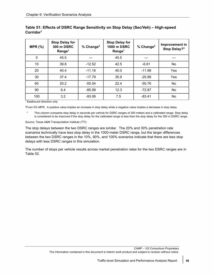
Chapter 6: Verification Scenarios Analysis
CAMP – V2I Consortium Proprietary The information contained in this document is interim work product and subject to revision without notice.
Traffic-level Simulation and Performance Analysis Report | 98
Table 51: Effects of DSRC Range Sensitivity on Stop Delay (Sec/Veh) – High-speed Corridor1
MPR (%) Stop Delay for 300 m DSRC
Range1 % Change2
Stop Delay for 1000 m DSRC
Range1 % Change2 Improvement in
Stop Delay?3
0 45.5 — 45.5 — —
10 39.8 -12.52 42.5 -6.61 No
20 40.4 -11.16 40.0 -11.99 Yes
30 37.4 -17.79 35.9 -20.99 Yes
60 20.2 -55.54 22.4 -50.76 No
90 6.4 -85.99 12.3 -72.87 No
100 3.2 -93.06 7.5 -83.41 No 1 Eastbound direction only 2From 0% MPR. A positive value implies an increase in stop delay while a negative value implies a decrease in stop delay
3 This column compares stop delay in seconds per vehicle for DSRC ranges of 300 meters and a calibrated range. Stop delay is considered to be improved if the stop delay for the calibrated range is less than the stop delay for the 300 m DSRC range.
Source: Texas A&M Transportation Institute (TTI)
The stop delays between the two DSRC ranges are similar. The 20% and 30% penetration rate scenarios technically have less stop delay in the 1000-meter DSRC range, but the larger differences between the two DSRC ranges in the 10%, 90%, and 100% scenarios indicate that there are less stop delays with less DSRC ranges in this simulation.
The number of stops per vehicle results across market penetration rates for the two DSRC ranges are in Table 52.

Chapter 6: Verification Scenarios Analysis
CAMP – V2I Consortium Proprietary The information contained in this document is interim work product and subject to revision without notice.
Traffic-level Simulation and Performance Analysis Report | 99
Table 52: Effects of DSRC Range Sensitivity on Number of Stops – High-speed Corridor1
MPR (%) # of Stops with
300 m DSRC Range
% Change2 # of Stops with 1000 m DSRC
Range % Change2 Improvment in #
of Stops?3
0 2.85 — 2.85 — —
10 3.04 6.51 2.95 3.39 Yes
20 3.10 8.70 3.34 17.27 No
30 3.62 26.80 3.58 25.73 Yes
60 3.80 33.36 3.45 20.87 Yes
90 1.16 -59.29 1.71 -40.09 No
100 0.59 -79.24 0.65 -77.24 Yes 1 Eastbound direction only 2 From 0% MPR. A positive value implies an increase in the number of stops while a negative value implies a decrease in the number of stops 3. This column compares the number of stops for DSRC ranges of 300 meters and a calibrated range. The number of stops is considered to be improved if the number of stops for the calibrated range is less than the number of stops for the 300 m DSRC range. Source: Texas A&M Transportation Institute (TTI)
The number of stops results for the two DSRC ranges do not show any clear trend for increased DSRC range performing better than the limited range. Rather, some of the penetration rate scenarios perform better with increased range and other scenarios perform worse. Note that the largest difference in the number of stops per vehicle between the DSRC ranges is the 90% scenario with a 0.55 stops per vehicle difference which is not a very large value.
Table 53 contains the differences in average speeds between the two DSRC ranges.

Chapter 6: Verification Scenarios Analysis
CAMP – V2I Consortium Proprietary The information contained in this document is interim work product and subject to revision without notice.
Traffic-level Simulation and Performance Analysis Report | 100
Table 53: Effects of DSRC Range Sensitivity on Average Speed (mph) – High-speed Corridor1
MPR (%) Average Speed for 300 m DSRC
Range % Change2
Average Speed for 1000 m
DSRC Rang % Change2 Improvement in
Avg Speed? 3
0 41.9 — 41.9 — —
10 42.0 0.13 41.7 -0.56 No
20 41.5 -1.03 41.4 -1.25 No
30 41.1 -1.87 41.1 -1.89 None
60 40.9 -2.54 40.7 -2.99 No
90 41.2 -1.82 40.4 -3.69 No
100 41.1 -2.05 40.5 -3.50 No 1 Eastbound direction only 2 From 0% MPR. A positive value implies an increase in average speed while a negative value implies a decrease in average speed 3. This column compares the average speed for DSRC ranges of 300 meters and a calibrated range. The average speed is considered to be improved if the average speed for the calibrated range is greater than the average speed for the 300 m DSRC range.
Source: Texas A&M Transportation Institute (TTI)
The average speeds for the increased DSRC range are consistently lower than the lower DSRC range. This makes sense because with increased DSRC range TOSCo vehicles have additional space to travel at a speed equal to or less than the speed limit to arrive at the intersection during the green window. This also means that with increased DSRC range, the vehicles with a set speed above the speed limit must reduce speeds so that their travel speeds are within the speed limit, contributing to lower average speeds on SH 105. Note that the differences in average speeds due to increased DSRC range are not very large and do not ever exceed one mile per hour in magnitude.
The impacts that DSRC range has on total travel times are shown in Table 54. Increased DSRC range shows less of an increase in Total Travel Time at lower market penetrations than the lower range DSRC. However, at higher market penetrations the total delay experiences a larger increase with larger DSRC range.
Table 54: Effects of DSRC Range Sensitivity on Total Travel Time (vehicle-hours) – High-speed Corridor1
MPR (%) Total Travel
Time for 300 m DSRC Range
% Change2 Total Travel
Time for 1000 m DSRC Range
% Change2 Improvement in Total Travel Time?3
0 1486 — 1486 -— —
10 1506 1.32 1494 0.50 Yes
20 1519 2.19 1507 1.40 Yes
30 1540 3.59 1516 1.97 Yes

Chapter 6: Verification Scenarios Analysis
CAMP – V2I Consortium Proprietary The information contained in this document is interim work product and subject to revision without notice.
Traffic-level Simulation and Performance Analysis Report | 101
MPR (%) Total Travel
Time for 300 m DSRC Range
% Change2 Total Travel
Time for 1000 m DSRC Range
% Change2 Improvement in Total Travel Time?3
60 1552 4.38 1542 3.76 Yes
90 1545 3.92 1565 5.31 No
100 1550 4.30 1566 5.37 No 1 Eastbound direction only 2 From 0% MPR. A positive value implies an increase in total travel time while a negative value implies a decrease in total travel time 3. This column compares the total travel time for DSRC ranges of 300 meters and a calibrated range. The total travel time is considered to be improved if the total travel time for the calibrated range is less than the total travel time for the 300 m DSRC range.
Source: Texas A&M Transportation Institute (TTI)
Table 55 shows the impacts of CO2 emissions.
Table 55: Effects of DSRC Range Sensitivity on CO2 Emissions (g/mi) – High-speed Corridor1
MPR (%) CO2 Emissions for 300 m DSRC
Range % Change2
CO2 Emissions for 1000 m
DSRC Range % Change2 Improvement in
CO2 Emissions?3
0 313.6 — 313.6 — —
10 307.7 -1.87 310.3 -1.07 No
20 308.6 -1.60 312.8 -0.27 No
30 317.2 1.14 319.1 1.74 No
60 316.9 1.05 317.1 1.11 No
90 314.4 0.24 311.1 -0.78 Yes
100 309.2 -1.40 313.8 0.07 No 1 Eastbound direction only
2 From 0% MPR. A positive value implies an increase in CO2 emissions while a negative value implies a decrease in CO2 emissions
3 This column compares the CO2 emissions for DSRC ranges of 300 meters and 100 meters. CO2 emissions is considered to be improved if CO2 emissions for the 1000 m range is less than CO2 emissions for the 300 m DSRC range.
Source: Texas A&M Transportation Institute (TTI)
The DSRC sensitivity analysis for the high-speed corridor shows that increased DSRC range does not consistently improve TOSCo function. Increased DSRC range tends to have worse performance than the 300-meter range at high market penetration. The research time attributes this to how the Infrastructure algorithm does not use a predicted queue length to determine a green window but the current queue length. This means that with increased DSRC range TOSCo vehicles receive information that may not be

Chapter 6: Verification Scenarios Analysis
CAMP – V2I Consortium Proprietary The information contained in this document is interim work product and subject to revision without notice.
Traffic-level Simulation and Performance Analysis Report | 102
relevant to the vehicle because the queue lengths might grow, or the signal actuation may gap out4 the side street while the TOSCo vehicle is approaching.
6.2.5 Discussion of Performance Results Overall total delay increases for the traffic on SH 105 as market penetration of TOSCo goes up. However, this is because TOSCo vehicles have more delay inherently. They accelerate gradually, to conserve fuel, and they will decelerate earlier than non-TOSCo vehicles on an approach. The trends for TOSCo and non-TOSCo individual vehicle classes identifies no change in total delay or a slight decrease in total delay. This means that TOSCo vehicles are not affecting total delay for non-TOSCo vehicles in low market penetrations and are reducing the delay for non-TOSCo vehicles at higher market penetrations.
TOSCo significantly reduces stop delay for all vehicle types at market penetration increases. This is one of the primary functions of the TOSCo system, therefore, the research team expected reductions in stop delay.
As TOSCo market penetration increased, the emissions rates at high speed remained constant. Figure 67, from a UCR study, shows that at average speeds of about 40 mph the emission rates tend to be constant as the average speeds change.
Source: Barth and Boriboonsomsin (24)
4 Gap out refers to the terminating of a green phase due to an excessive time interval between the actuations of vehicles arriving on the green, so green may be served to a competing phase.

Chapter 6: Verification Scenarios Analysis
CAMP – V2I Consortium Proprietary The information contained in this document is interim work product and subject to revision without notice.
Traffic-level Simulation and Performance Analysis Report | 103
Figure 67: CO2 Emissions Rates Across Average Speeds
Some of the trends between the high-speed corridor and the low-speed corridor do not match. The emissions rates on SH 105 reside in a speed range where the real-world activity curve in Figure 67 is horizontal. This means that five or ten mph changes on average, will not drastically impact the emission rate for SH 105. For this reason, the research team crafted an additional simulation experiment to better understand the impacts of TOSCo on a higher speed corridor. This experiment involved using a modification of the Coordinated Stop Verification Scenario, which includes vehicles accelerating from a complete stop. However, this is not a coordinated stop. This experiment involves completely stopped vehicles accelerating to their desired speed. The modification enabled the research team to observe the differences between the non-TOSCo vehicles using the VISSIM default acceleration and TOSCo vehicles as they accelerate to a low set speed, 15 meters per second (34 mph), and a high set speed, 25 meters per second (56 mph). Figure 68 shows the speed profiles for the two driving speeds in this experiment.
(a) Low Set Speed (b) High Set Speed
Source: Crash Avoidance Metrics Partners LLC (CAMP) Vehicle to Infrastructure (V2I) Consortium
Figure 68: Speed Profile Comparison Between TOSCo and Non-TOSCo at Different Speeds
At both set speeds TOSCo vehicles require more time to accelerate than the non-TOSCo vehicles. However, at the low-set speed, the difference in time for the TOSCo vehicles to reach speed compared to the Non-TOSCo vehicles is not as extreme as the high set speed. TOSCo vehicles require eight and over 20 additional seconds than the baseline traffic to accelerate to the low and high set speeds, respectively. The research team determined that this experiment revealed two future research needs. First, the non-TOSCo vehicles are accelerating too aggressively. The VISSIM default acceleration profile (shown in Figure 42) produces high accelerations early in the acceleration process, when compared with recent research on the topic of typical acceleration levels (28). Second, the TOSCo algorithm for launching behavior does not provide sufficient acceleration as currently designed, especially with high set speeds. The research team must revisit the TOSCo algorithm to accelerate vehicles to their set in less time than the trigonometric functions used in this study.

Chapter 6: Verification Scenarios Analysis
CAMP – V2I Consortium Proprietary The information contained in this document is interim work product and subject to revision without notice.
Traffic-level Simulation and Performance Analysis Report | 104
The TTI team performed an initial analysis of the impacts of using a faster launch algorithm by implementing the Intelligent Driver Model (IDM) (7,8) to control the Coordinated Launch behavior. Figure 69 shows that the IDM accelerated faster than the TOSCo launch method used for the primary analysis in the beginning of the acceleration process, even though both methods did not bring the TOSCo vehicle completely to speed as fast as the non-TOSCo vehicles.
Source: Crash Avoidance Metrics Partners LLC (CAMP) Vehicle to Infrastructure (V2I) Consortium
Figure 69: Comparison between TOSCo, Non-TOSCo and TOSCo Launch Revision at High Speeds
The TTI team conducted some preliminary simulations to observe the potential impacts of improving the TOSCo launch speed, using a single seed for each market penetration rate. Figure 70 and Table 56 contain the results for the eastbound, peak, direction for SH 105 using the revised TOSCo launch.
Source: Texas !&M Transportation Institute (TTI)
0.00
5.00
10.00
0.0
100.0
200.0
0% 20% 40% 60% 80% 100%
Num
ber o
f Sto
ps (#
/veh
)
Aver
age
Dela
y (s
/veh
)
TOSCo Market Penetration Rate
Corridor Level Mobility Measurement for Eastbound Direction (All Vehicles, Revised TOSCo Launch)
Total Delay Stop Delay Number of Stops

Chapter 6: Verification Scenarios Analysis
CAMP – V2I Consortium Proprietary The information contained in this document is interim work product and subject to revision without notice.
Traffic-level Simulation and Performance Analysis Report | 105
Figure 70: Corridor Level Measurement of Mobility in Eastbound Direction with Revised TOSCo Launch (All Types)
Table 56: Mobility Comparison at Corridor Level – Eastbound Direction with Revised TOSCo Launch
MPR (%) Total Delay (sec/veh) % Change1 Stop Delay
(sec/veh) % Change1 # of Stops / Vehicle % Change1
0 126.7 — 43.3 — 2.84 —
10 117.1 -7.5 39.2 -9.6 2.83 -0.3
20 136.1 7.4 40.6 -6.3 3.42 20.4
30 138.2 9.1 36.6 -15.4 3.71 30.7
60 132.1 4.3 20.3 -53.1 3.64 28.1
90 126.4 -0.2 7.4 -82.8 1.46 -48.6
100 123.7 -2.3 2.8 -93.4 0.60 -78.7 1 From 0% MPR. A positive value implies an increase while a negative value implies a reduction in the performance measure
Source: Texas A&M Transportation Institute (TTI)
With the IDM Coordinated Launch, the TOSCo vehicles experienced a slight increase in total delay in the intermediate market penetration rates and slight decreases in total delay at low and high market penetration rates. The trends for stop delay and number of stops are like the results from the primary analysis. Since this experiment only used one seed for each scenario, these results only represent a ballpark estimate of the decreases and increases in total delay. However, these results show that revising the TOSCo launch behavior can reduce the total delay TOSCo vehicles experience compared to the primary analysis. Furthermore, the revision shows that revising the Coordinated Launch behavior can lead to similar total delay values as the baseline traffic.
For brevity, the research team excluded the results from this experiment for the westbound mobility, travel time, average speed, and emissions. The westbound mobility results were very similar to the eastbound mobility results with reduced total delays at higher market penetration rates and no difference in the stop delay and number of stops compared to the primary analysis. The trends in travel time and average speed in this experiment were the same as the primary analysis. Total travel time increased and average speeds decreased as market penetrations increased. Finally, the emission results remained constant across market penetration rates, like in the primary analysis.
This experiment confirms that adjusting the TOSCo launch behavior to something that provides more acceleration early in the process than the trigonometric functions will aid in addressing the magnitude of total delay increases seen in the high-speed corridor. TOSCo vehicles should not necessarily use the IDM model to accelerate from a stopped position. Instead, the research team should work together to determine the most appropriate methodology for TOSCo vehicles to accelerate from a stop.

Chapter 6: Verification Scenarios Analysis
CAMP – V2I Consortium Proprietary The information contained in this document is interim work product and subject to revision without notice.
Traffic-level Simulation and Performance Analysis Report | 106
6.2.6 Monetization of Results The high-speed corridor utilized the same methodology for assessing the user costs at different market penetration rates as the low-speed corridor. However, the research team used $2.01 per gallon, which was the average fuel costs in Texas in December 2018 (26). Table 57 contains the costs of total travel time and fuel for the SH 105 Corridor.
Table 57: SH 105 Corridor User Cost Analysis
Penetration Rate Value of Total Travel Time
Fuel Cost (Texas Gasoline Price, 2018) Total User Costs
0 $ 12,858.15 $6,650.95 $ 19,509.10
10 $ 12,925.13 $6,601.89 $ 19,527.02
20 $ 12,987.86 $6,658.21 $ 19,646.07
30 $ 13,066.87 $6,740.56 $ 19,807.43
60 $ 13,192.81 $6,726.21 $ 19,919.02
90 $ 13,375.54 $6,663.22 $ 20,038.76
100 $ 13,447.03 $6,617.34 $ 20,064.37 Source: Texas A&M Transportation Institute (TTI)
The user costs steadily increase between the baseline and the 100% market penetration rate up to about a $550 user increase in costs. The increases are caused by increased travel time and the minimal changes in fuel costs with the evaluated version of TOSCo.
6.2.7 Traffic-level Simulation Reassessments and Refinements As part of the initial infrastructure simulations, the research team reevaluated some of the results and made some refinements associated with the default acceleration profile governing vehicle behaviors by enhancing the representation of non-TOSCo vehicles on the high-speed corridor. To accomplish this, the team designed an acceleration study to collect acceleration behaviors on the State Highway (SH) 105 corridor and provide data needed to generate a revised acceleration distribution for the non-TOSCo vehicles within VISSIM. The team used this revised acceleration distribution to evaluate the impacts of TOSCo compared to the refined representation of baseline traffic.
6.2.7.1 SH 105 Acceleration Profile Development
Information on the acceleration behavior from DSRC vehicles was not available for the high-speed corridor, leading the team to use the default desired acceleration distribution provided in VISSIM. Figure 71 shows the VISSIM default acceleration distribution and Figure 72 shows the calibrated vehicle acceleration profile by UMTRI from acceleration events on Plymouth Rd. using naturalistic driving data (NDD) [19]. The VISSIM default accelerations for the non-equipped vehicles is more aggressive than the naturalistic data from Plymouth Rd. The VISSIM profile averages at 10 ft/s2 acceleration from a stop while the NDD profile averages at 5.5 ft/s2. This large difference in the acceleration behaviors from a stop suggested to the research team that the acceleration behavior by the vehicles on SH 105 is different than the VISSIM default acceleration profile. However, as the posted speed limit on SH 105 is 55 mph, the NDD profile does not cover speeds high enough to represent SH 105. The research team determined

Chapter 6: Verification Scenarios Analysis
CAMP – V2I Consortium Proprietary The information contained in this document is interim work product and subject to revision without notice.
Traffic-level Simulation and Performance Analysis Report | 107
that more work needed to be done to better represent the acceleration behavior of the traffic on SH 105 to compare to the simulated TOSCo behavior, so the research team designed a study to collect the acceleration data needed to create a profile to represent SH 105 acceleration behavior.
Source: PTV VISSIM
Figure 71: VISSIM Default Acceleration Distribution to Model Accelerations of Non-TOSCo Vehicles
Source: University of Michigan Transportation Research Institute (UMTRI)
Figure 72: Acceleration Profile Calibrated from Naturalistic Driving Data [19]
The graphs in Figure 71 and Figure 72 describe the acceleration behavior of a VISSIM controlled vehicle that wants to gain speed to its randomly assigned desired speed. As VISSIM controls vehicles it will follow either minimum, median, or maximum acceleration pattern until the vehicle reaches its desired
0
5
10
15
0 20 40 60 80 100 120 140 160 180Acce
lera
tion
(ft/s
ec^2
)
Speed (mph)
VISSIM Default Desired Acceleration Functions (English Unit)
AccMedian AccMin AccMax
-1
4
9
14
0 20 40 60 80 100 120 140 160 180Acce
lera
tion
(ft/s
ec^2
)
Speed (mph)
Naturalistic Driving Data Acceleration Functions from Plymouth Rd.
AccMedian AccMin AccMax

Chapter 6: Verification Scenarios Analysis
CAMP – V2I Consortium Proprietary The information contained in this document is interim work product and subject to revision without notice.
Traffic-level Simulation and Performance Analysis Report | 108
speed and the acceleration drops to zero. If the acceleration profile extends beyond a vehicles desired speed, which is the case for the simulated SH 105 vehicles using the VISSIM default acceleration profile, the vehicle tracks the acceleration profile until reaching its desired speed and then stops accelerating. Therefore, the VISSIM default acceleration profile allows simulated vehicles on SH 105 to reach their desired speeds above 50 mph, but the NDD profile does not because all of the desired acceleration trends reach zero at 50 mph.
The research team designed and conducted an acceleration study to collect the representative acceleration behaviors on SH 105. The study used a segment of SH 105 between Old River Road and April Sound Boulevard shown in Figure 73. The research team selected this segment for the 2.5 mile interval between these two intersections, which allowed traffic to accelerate completely to their desired speed without an upstream intersection affecting their behavior.
Source: Imagery ©2019 Google. Map Data ©2019 Google
Figure 73: Study Segment on SH 105
This acceleration study used two vehicles, each equipped with a Xsens’ MTi-G-710 sensor package. The Xsens’ MTi-G-710 is a high-performance sensor system with accuracies surpassing conventional Attitude and Heading Reference System (AHRS) and Micro-Electro Mechanical Systems (MEMS) inertial sensors. It measures the acceleration and speed directly. To complement the data recorded by the sensor, each driver kept a field log. In the field log, each driver noted if they approached an intersection during a red phase, reached a completed stop and position in the queue. When the signal turned green the study driver accelerated so that they paced with the vehicle ahead. If the study vehicle was the leading vehicle in the queue, they could either accelerate to pace with the leading vehicle in the adjacent lane or accelerate at their own comfort. Twenty three hours of data were collected during this study between the two vehicles amounting to about 150 acceleration events recorded.
The sensor measured acceleration and speed in three axis on a fixed coordinate system defined with the x-axis positive to the East, y-axis positive to the North, and z-axis positive pointing up (see Figure 74). The device recorded data at a rate of 400 Hz.

Chapter 6: Verification Scenarios Analysis
CAMP – V2I Consortium Proprietary The information contained in this document is interim work product and subject to revision without notice.
Traffic-level Simulation and Performance Analysis Report | 109
Source: Texas A&M Transportation Institute (TTI)
Figure 74: Acceleration Sensor Orientation Compared to SH 105
The team calculated the acceleration and speed of the vehicle using the following equations:
𝑣𝑣 = �𝑣𝑣𝑥𝑥2 + 𝑣𝑣𝑦𝑦2
Figure 75: Vehicle Speed
𝑎𝑎𝐸𝐸𝐸𝐸 = �𝑎𝑎𝑥𝑥2 + 𝑎𝑎𝑦𝑦2 ∗ 𝑠𝑠𝑔𝑔𝑠𝑠(𝑎𝑎𝑥𝑥)
Figure 76: Acceleration Eastbound
𝑎𝑎𝑊𝑊𝐸𝐸 = −�𝑎𝑎𝑥𝑥2 + 𝑎𝑎𝑦𝑦2 ∗ 𝑠𝑠𝑔𝑔𝑠𝑠(𝑎𝑎𝑥𝑥)
Figure 77: Acceleration Westbound
Where, 𝑣𝑣𝑥𝑥 , 𝑣𝑣𝑦𝑦 , 𝑎𝑎𝑥𝑥 , 𝑎𝑎𝑦𝑦 are speed and acceleration in the x and y axes of the fixed coordinate system. Note that, the sensor measures acceleration from the texture of the road and changes in grade in the z-direction, which is not valuable data for the acceleration profile. The rotation across the z-axis indicated the vehicle changing directions and orientation indicated the direction of travel within the data so the algorithm used to analyze the data could select the appropriate equation for calculating the acceleration.

Chapter 6: Verification Scenarios Analysis
CAMP – V2I Consortium Proprietary The information contained in this document is interim work product and subject to revision without notice.
Traffic-level Simulation and Performance Analysis Report | 110
The research team cleaned the acceleration data to reduce the noise in the data and smooth out human error in the data set. The team tried several methods to reduce noise and concluded that local weighting with a 0.05% sampling yield properly smoothed the data and removed human error within the data set while maintaining enough sensitivity to changes in acceleration to capture the acceleration behavior well. The team created a script to automatically identify acceleration events from a stop and clean the data. Next, an analyst cross checked each acceleration profile that was with the field logs to use only events where the study vehicle was the first or second vehicle in the queue. The acceleration distribution for VISSIM was based on the maximum, median, and minimum accelerations at different speeds from the resulting 73 valid profiles. The resulting calibrated SH 105 VISSIM acceleration distribution is shown in Figure 78.
Source: Texas A&M Transportation Institute (TTI)
Figure 78: Acceleration Profile Calibrated from SH 105 Field Study
The profile is similar in shape to the calibrated acceleration profile from the NDD [19]. This profile has less acceleration from a stop but greater accelerations at higher speeds than the low speed corridor. The team did not allow the minimum desired acceleration to reach zero, so vehicles that follow the minimum acceleration behavior are always able to accelerate, if desired. Additionally, the team extended the minimum, median, and maximum curves up to 150 mph to allow vehicles to accelerate to desired speeds beyond the acceleration profile. These two edits ensured that all VISSIM controlled vehicles could accelerate to their desired speed.
The calibrated VISSIM acceleration profile has a wider range of speed compared to the profile for the low speed corridor, due to the higher speeds on SH 105. Moreover, the calibrated VISSIM acceleration is different from the VISSIM default acceleration profile at every speed range demonstrated in Table 58.

Chapter 6: Verification Scenarios Analysis
CAMP – V2I Consortium Proprietary The information contained in this document is interim work product and subject to revision without notice.
Traffic-level Simulation and Performance Analysis Report | 111
Table 58: Comparisons on Averaged Acceleration for VISSIM Default and SH 105 Acceleration Profiles
Speed Range Average VISSIM Default Acceleration (ft/s^2)
Average SH 105 Acceleration (ft/s^2) Difference (ft/s2)
0-30 mph 8.9 6.2 2.6
30-50 mph 5.6 5.9 -0.3
50-70 mph 4.3 3.6 0.7
70-100 mph 3.6 1.3 2.3
100+mph 1.6 0.7 1.0 Source: Texas A&M Transportation Institute (TTI)
The revised VISSIM acceleration profile has an average of 2.9 ft/s2 acceleration from stop, which builds up to 7.5 ft/s2 as the vehicle gains speed, similar to the NDD profile. The revised profile reflects behavior observed from the field study where vehicles accelerated gradually from a stop and maintained acceleration until reaching their desired speeds.
6.2.7.2 Model Recalibration for Travel Times
Travel time was a calibration parameter for this model, so the research team checked to see how much this performance measure changes and recalibrated the model. The research team found that travel time results from the SH 105 model are larger with the revised acceleration distribution than with the default acceleration distribution. The travel time values from the original travel time study conducted for TOSCo in 2017, the revised simulated travel times through the corridor, and the differences in percentage are tabulated in Table 59. The travel times in the simulation are larger than the field data in both directions, especially for the eastbound direction, which exceeds the calibration target of a 10% difference from the field data. Therefore, the team needed to recalibrate the SH 105 model to bring the simulated travel times closer to the field data.
Table 59: Comparisons between 2017 Field Data and Simulated Travel Times before Recalibration in the AM Peak
Direction of Travel 2017 Field Data (sec)
Simulated Travel Time with Revised Acceleration Profile Difference (%)
Eastbound 803.0 998.7 24.4*
Westbound 842.9 909.9 7.9 * Difference exceeds 10% threshold for recalibration.
Source: Texas A&M Transportation Institute (TTI)
The research team decided to do another travel time study since the previous travel time data was collected before two intersections modeled on the SH 105 corridor were signalized, which could affect the travel times on the facility. The travel time study in 2019 used one vehicle and a floating car method in the AM and PM peak periods, like the study in 2017. The travel time measurements from the field are documented in Table 60.

Chapter 6: Verification Scenarios Analysis
CAMP – V2I Consortium Proprietary The information contained in this document is interim work product and subject to revision without notice.
Traffic-level Simulation and Performance Analysis Report | 112
Table 60: Summary of AM Peak Travel Times from 2017 and 2019 Studies
Direction of Travel 2017 Field Data (seconds) 2019 Field Data (seconds) Difference (sec)
Eastbound 803.0 879.0 76.0
Westbound 842.9 893.3 50.4 Source: Texas A&M Transportation Institute (TTI)
The travel time study conducted in 2017 had six runs in both eastbound and westbound directions for the AM and PM peak periods while the 2019 study has three runs in both directions for the AM peak, and four runs in both directions for the PM peak. The research team performed a statistical analysis to test if the mean travel times for the 2017 and 2019 studies are different. The analysis showed that the differences in travel times recorded in 2017 and 2019 are not statistically significant despite increased travel times for both directions in the 2019 data—i.e., 76-second increase in the eastbound and 50.4-second increase in the westbound directions. However, the simulated travel times still exceeded the 10% calibration threshold with the 2019 field data, (see Table 61). When calibrating a microscopic model, a goal must be defined to determine if the model is sufficiently representative for the data to be valid. The research team endeavored to remain within the 10% calibration threshold to ensure that the model is realistic.
Table 61: Travel Times Before and After Recalibration
Direction of Travel
2019 Field Measured
Travel Time (sec)
Simulated Travel Times with Default Acceleration Profile
(sec)
Difference (%)
Simulated Travel Times with Revised Acceleration Profile
(sec)
Difference (%)
Eastbound 879.0 998.7 13.6 908.4 3.3
Westbound 893.3 909.9 1.8 904.3 1.2 Source: Texas A&M Transportation Institute (TTI)
To decrease the travel time from simulation for recalibration, the research team then modified the desired speed profile in VISSIM for the baseline traffic as shown in Figure 79. The recalibration effort increased the average speeds of vehicles to match the travel times recorded in the field. Both AM and PM peak simulations used the recalibrated desired speed distribution in Figure 79.

Chapter 6: Verification Scenarios Analysis
CAMP – V2I Consortium Proprietary The information contained in this document is interim work product and subject to revision without notice.
Traffic-level Simulation and Performance Analysis Report | 113
Source: Texas A&M Transportation Institute (TTI)
Figure 79: Speed Profiles for Before and After Recalibration
With the recalibrated model, the travel times from simulations are close to the travel times collected in field study and within the 10% difference (See Table 61).
6.2.7.3 Revised AM Peak Performance Results
The research team selected a reduced number of Market Penetration Rates (MPR) and simulation seeds to run to expedite the process. The team decided to use the baseline, 30, 60, and 100% TOSCo MPRs because previous simulation delay results were typically flat between these MPRs. Each scenario used the same parameters as before, with a 900 second warm-up period and a 7200 second evaluation period for each of the five simulation seeds in these refined results. The eastbound and westbound AM peak revised results are shown in Figure 80, Figure 81, Table 62 and Table 63, respectively.

Chapter 6: Verification Scenarios Analysis
CAMP – V2I Consortium Proprietary The information contained in this document is interim work product and subject to revision without notice.
Traffic-level Simulation and Performance Analysis Report | 114
Source: Texas A&M Transportation Institute (TTI)
Figure 80: AM Peak Revised Corridor-Level Mobility Measures for SH 105 (Eastbound)—All Vehicle Types
Table 62: Revised Mobility Comparison at the Corridor Level in the AM Peak– All Vehicle Types (Eastbound Direction)
MPR (%) Total Delay (sec/veh) % Change1 Stop Delay
(sec/veh) % Change1 # of Stops / Vehicle % Change1
0 153.2 - 45.6 - 2.82 -
30 199.9 30.5 42.6 -6.6 5.33 89.0
60 205.6 34.2 26.7 -41.5 4.39 55.5
100 213.1 39.1 9.9 -78.4 0.87 -69.3 1 From 0% MPR. A positive value implies an increase while a negative value implies a reduction in the performance measure
Source: Texas A&M Transportation Institute (TTI)
0
2
4
6
8
10
12
14
0
50
100
150
200
250
300
350
400
0 10 20 30 40 50 60 70 80 90 100
Num
ber o
f Sto
p (#
/veh
)
Aver
age
Dela
y (s
/veh
)
TOSCo Market Penetration Rate (%)
AM Peak SH 105 Revised Corridor-level Mobility Measurements for Eastbound Direction
Total Delay Stop Delay Number of Stops

Chapter 6: Verification Scenarios Analysis
CAMP – V2I Consortium Proprietary The information contained in this document is interim work product and subject to revision without notice.
Traffic-level Simulation and Performance Analysis Report | 115
Source: Texas A&M Transportation Institute (TTI)
Figure 81: AM Peak Revised Corridor-Level Mobility Measures for SH 105 (Westbound)—All Vehicle Types
Table 63: Revised Mobility Comparison at the Corridor Level in the AM Peak– All Vehicle Types (Westbound Direction)
MPR (%) Total Delay (sec/veh) % Change1 Stop Delay
(sec/veh) %Change1 # of Stops / Vehicle % Change1
0 126.9 - 46.4 - 2.820213 -
30 145.8 15% 35.1 -24% 2.483973 -11.9
60 157.2 24% 20.9 -55% 1.493351 -47.0
100 162.2 28% 4.4 -90% 0.342429 -87.9 1 From 0% MPR. A positive value implies an increase while a negative value implies a reduction in the performance measure
Source: Texas A&M Transportation Institute (TTI)
The AM peak results for total delay, stop delay, and number of stops follow the same trends as they did before revising the model. In the eastbound direction, total delay increased from 153.2 seconds to 213.1 seconds and from 126.9 seconds to 162.2 seconds in the westbound direction. The differences are 59.9 seconds and 35.3 seconds, respectively which are greater increases than before the revision. These increases are caused by the recalibration bringing the desired speeds of the corridor to values higher than before. Many simulated vehicles have desired speeds above the speed limit, which causes TOSCo vehicles to reduce their speeds when they enter communication range as the algorithm currently forces TOSCo vehicles to adhere to the speed limit, their delays increase (recall delay is defined as the difference between a vehicle’s theoretical uninterrupted travel time at its prevailing speed during the peak period and its simulated travel time). In addition, TOSCo vehicles require a longer time to accelerate to their desired speeds from a stop because this simulation uses the first generation TOSCo speed profiles,

Chapter 6: Verification Scenarios Analysis
CAMP – V2I Consortium Proprietary The information contained in this document is interim work product and subject to revision without notice.
Traffic-level Simulation and Performance Analysis Report | 116
which accelerate to large speeds by increasing time spent building up to the maximum acceleration instead of increasing the amount of time at the maximum acceleration.
The trends observed in stop delay and number of stops are similar to the previous AM peak period results for SH 105 and have the same explanation. Increased stops in the eastbound direction are a result of non-TOSCo vehicles stopping briefly in response to TOSCo vehicle driving behavior. There is a steady, and significant, decrease in stop delay as MPR increases.
Figure 82 and Table 64 show the total travel time and average speed results from the AM peak SH 105 revision. There are slight decreases in average speed and increases in total travel times across all MPRs. The changes in total travel time and average speeds for all vehicles in the network are slight.
Source: Texas A&M Transportation Institute (TTI)
Figure 82: Total Vehicle Hours Traveled and Average Speeds for High-speed Corridor AM Peak Revision
Table 64: Total Vehicle Hours Traveled and Average Speeds for High-speed Corridor AM Peak Revision
MPR (%) Total Travel Time (veh-hrs) %Change1 Avg Speed (mph) % Change1
0 889 - 46.2 -
30 902 1.5 45.6 -1.3
60 936 5.2 44.2 -4.4
100 918 3.3 45.5 -1.7 1 From 0% MPR. A positive value implies an increase while a negative value implies a reduction in the performance measure
Source: Texas A&M Transportation Institute (TTI)
0
10
20
30
40
50
0
200
400
600
800
1000
1200
0 10 20 30 40 50 60 70 80 90 100
Aver
age
Spee
d (m
ph)
Tota
l Tra
vel T
ime
(veh
-hou
r)
TOSCo Market Penetration Rate (%)
Total Travel Time and Average Speed
Total Travel Time Average Speed

Chapter 6: Verification Scenarios Analysis
CAMP – V2I Consortium Proprietary The information contained in this document is interim work product and subject to revision without notice.
Traffic-level Simulation and Performance Analysis Report | 117
The emissions results for the AM peak revision are in Figure 83 and Table 65. Emissions and energy rates increase slightly in the 30% and 60% MPRs and return to values similar to the baseline at the 100% MPR scenario. These changes are likely caused by the increases in stops and the slight changes in average speed, since the MOVES model is very sensitive to changes in speeds. The team needs to investigate environmental impacts in the high-speed corridor further in future work.
Source: Texas A&M Transportation Institute (TTI)
Figure 83: CO2 Emissions and Energy Usage Rates for High-speed Corridor AM Peak Revision
Table 65: Emissions and Energy use across TOSCo MPRs for High-speed Corridor AM Peak Revision
MPR (%) CO2 Emissions (g/veh-mi) % Change1 Total Energy (kJ/veh-mi) % Change1
0 710 - 9,786 -
30 748 5.3 10,305 5.3
60 743 4.6 10,235 4.6
100 714 0.4 9,830 0.4 1 From 0% MPR. A positive value implies an increase while a negative value implies a reduction in the performance measure
Source: Texas A&M Transportation Institute (TTI)
6.2.7.4 PM Peak Performance Results
The research team also used the revised acceleration distribution in the PM peak simulation for the SH 105 corridor. The PM peak conditions are over saturated in both directions at several intersections along SH 105. The traffic volumes in eastbound and westbound directions are more evenly distributed, and the eastbound direction is still the direction with the peak flow. Eastbound traffic remains the peak direction because the PM peak period involves trips to shopping locations along SH 105 in addition to commuter traffic. The PM peak simulation calibration for travel time is show in Table 66. Note, the eastbound travel time measurement exceeds the calibration target of 10% change from the field measurement and the westbound travel time measurement is within the calibration target.
020004000600080001000012000
0
200
400
600
800
0 10 20 30 40 50 60 70 80 90 100
Ener
gy (K
J/ve
h-m
i)
CO2
Emiss
ions
Rat
e (g
/veh
-mi)
TOSCo Market Penetration Rate (%)
CO2 and Energy Emissions
CO2 Energy

Chapter 6: Verification Scenarios Analysis
CAMP – V2I Consortium Proprietary The information contained in this document is interim work product and subject to revision without notice.
Traffic-level Simulation and Performance Analysis Report | 118
Table 66: Field Measured Travel Times and Travel Times After Recalibration
Direction of Travel
2019 Field Measured Travel Time (sec)
Simulated Travel Times w/ Revised Acceleration Profile (sec) % Change
Eastbound 951.7 1,108.8 16.5
Westbound 972.0 995.3 2.4 Source: Texas A&M Transportation Institute (TTI)
The PM peak simulation also used the baseline, 30, 60, and 100 MPRs and has one simulation seed for each scenario. The delay and number of stop results for eastbound and westbound directions of travel are shown in Figure 84 and Figure 85 and the values are shown in Table 67 and Table 68.
Source: Texas A&M Transportation Institute (TTI)
Figure 84: PM Peak Revised Corridor-Level Mobility Measures for SH 105 (Eastbound)—All Vehicle Types
Table 67: PM Peak Mobility Comparison at the Corridor Level – All Vehicle Types (Eastbound Direction)
MPR (%) Total Delay (sec/veh) %Change1 Stop Delay
(sec/veh) %Change1 # of Stops / Vehicle % Change1
0 376.0 - 137.1 - 9.3 -
30 317.4 -15.6 67.0 -51.1 7.8 -15.9
60 304.3 -19.1 34.4 -74.9 6.5 -30.6
100 312.2 -17.0 11.2 -91.8 1.5 -84.0 1 From 0% MPR. A positive value implies an increase while a negative value implies a reduction in the performance measure
Source: Texas A&M Transportation Institute (TTI)
02468101214
050
100150200250300350400
0 10 20 30 40 50 60 70 80 90 100
Num
ber o
f Sto
ps (#
/veh
)
Aver
age
Dela
y (s
/veh
)
TOSCo Market Penetration Rate (%)
PM Peak SH 105 Corridor-Level Mobility Meaures for Eastbound Traffic (All Vehicle Types)
Total Delay Stop Delay Number of Stops

Chapter 6: Verification Scenarios Analysis
CAMP – V2I Consortium Proprietary The information contained in this document is interim work product and subject to revision without notice.
Traffic-level Simulation and Performance Analysis Report | 119
Source: Texas A&M Transportation Institute (TTI)
Figure 85: PM Peak Revised Corridor-Level Mobility Measures for SH 105 (Westbound)—All Vehicle Types
Table 68: PM Peak Mobility Comparison at the Corridor Level – All Vehicle Types (Westbound Direction)
MPR (%) Total Delay (sec/veh) % Change1 Stop Delay
(sec/veh) % Change1 # of Stops / Vehicle % Change1
0 260.7 - 123.0 - 5.2 -
30 259.5 -0.4 75.9 -38.3 5.8 11.0
60 247.9 -4.9 34.2 -72.2 4.0 -23.1
100 230.6 -11.5 10.4 -91.6 0.8 -85.6 1 From 0% MPR. A positive value implies an increase while a negative value implies a reduction in the performance measure
Source: Texas A&M Transportation Institute (TTI)
The similar volumes and conditions in the two directions lead to similar results in the two directions in the PM peak scenario. Both directions experience gradual reductions in stop delay and number of stops as the market penetration of TOSCo increases. The westbound direction experiences a slight increase in number of stops between the baseline and 30% MPR and then consistently decreases in the other scenarios. Total delay per vehicle decreases significantly between the baseline and the 30% MPR scenario in the heavier eastbound direction and remains constant for the remaining scenarios.
The westbound direction experiences a slight increase in the number of stops between the baseline and 30% MPR and then consistently decreases in the other scenarios. The westbound stop delay gradually
0
2
4
6
8
10
12
14
0
50
100
150
200
250
300
350
400
0 10 20 30 40 50 60 70 80 90 100
Num
ber o
f Sto
ps (#
/veh
)
Aver
age
Dela
y (s
/veh
)
TOSCo Market Penetration Rate (%)
PM Peak SH 105 Corridor-Level Mobility Meaures for Westbound Traffic (All Vehicle Types)
Total Delay Stop Delay Number of Stops

Chapter 6: Verification Scenarios Analysis
CAMP – V2I Consortium Proprietary The information contained in this document is interim work product and subject to revision without notice.
Traffic-level Simulation and Performance Analysis Report | 120
decreases as MPR goes up. Total delay remains approximately constant between the baseline and the 30% MPR scenario and then gradually decreases in the 60% and 100% MPRs.
Figure 86 and Table 69 show the total travel time and average speed results from the PM peak. These measurements remain constant across increased TOSCo MPR, despite reductions in total delay for vehicles traveling from end-to-end of the corridor. This measurement includes vehicles on cross streets and turning movements, which indicates that, although there are marginal increases in travel speed for vehicles going end-to-end on SH 105, the overall average speeds for all users on SH 105 remains constant with increasing TOSCo MPR.
Source: Texas A&M Transportation Institute (TTI)
Figure 86: Total Vehicle Hours Traveled and Average Speeds for High-speed Corridor PM Peak Revision
Table 69: Total Vehicle Hours Traveled and Average Speeds for High-speed Corridor PM Peak
MPR (%) Total Travel Time (veh-hrs) % Change1 Avg Speed (mph) % Change1
0 984 - 40.6 -
30 997 1.3 40.2 -0.9
60 1011 2.7 40.1 -1.3
100 1016 3.2 40.3 -0.7 1 From 0% MPR. A positive value implies an increase while a negative value implies a reduction in the performance measure
Source: Texas A&M Transportation Institute (TTI)
0
10
20
30
40
50
0
200
400
600
800
1000
1200
0 10 20 30 40 50 60 70 80 90 100
Aver
age
Spee
d (m
ph)
Tota
l Tra
vel T
ime
(veh
-hou
r)
TOSCo Market Penetration Rate (%)
Total Travel Time and Average Speed
Total Travel Time Average Speed

Chapter 6: Verification Scenarios Analysis
CAMP – V2I Consortium Proprietary The information contained in this document is interim work product and subject to revision without notice.
Traffic-level Simulation and Performance Analysis Report | 121
The emission results for the PM peak period are in Figure 87 and Table 70. There is a slight reduction in emission rates and energy consumption at higher TOSCo MPR in the PM peak period. Like the AM peak emissions, these changes are small compared to the magnitude of the emission rates. The reduction in emissions for the PM peak simulation is consistent with the reductions in stops.
Source: Texas A&M Transportation Institute (TTI)
Figure 87: CO2 Emissions and Energy Usage Rates for High-speed Corridor PM Peak Revision
Table 70: Emissions and Energy Use across TOSCo MPRs for High-speed Corridor PM Peak
MPR (%) CO2 Emissions (g/veh-mi) % Change1 Total Energy (kJ/veh-mi) % Change1
0 643 - 8860 -
30 645 0.2 8879 0.2
60 638 -0.8 8786 -0.8
100 620 -3.6 8538 -3.6 1 From 0% MPR. A positive value implies an increase while a negative value implies a reduction in the performance measure
Source: Texas A&M Transportation Institute (TTI)
6.2.7.5 Discussion of Differences between AM and PM Peak Results for SH 105
The AM and PM peak periods have different trends in mobility measurements. This is primarily due to all intersections during the AM peak period being undersaturated and some intersections in the PM peak being saturated. None of the intersections during the AM peak period have average queue length behavior that indicate saturated conditions, meaning queue lengths continually grow longer over time until eventually demand decreases enough that the queue length begins to decrease. The PM peak does have saturated conditions at intersections, meaning that some vehicles in an eastbound or westbound
0
2000
4000
6000
8000
10000
12000
0
100
200
300
400
500
600
700
800
0 10 20 30 40 50 60 70 80 90 100
Ener
gy (K
J/m
i)
CO2
Emiss
ions
Rat
e (g
/veh
-mi)
TOSCo Market Penetration Rate (%)
CO2 and Energy Emissions
CO2 Energy

Chapter 6: Verification Scenarios Analysis
CAMP – V2I Consortium Proprietary The information contained in this document is interim work product and subject to revision without notice.
Traffic-level Simulation and Performance Analysis Report | 122
queue on SH 105 are not able to clear the intersection in the allotted green time for that phase. Figure 88 shows the queueing behavior for each MPR for a saturated movement in the PM peak period at Old River Rd. in the eastbound direction. There is a large reduction in delay and reduction in delays for vehicles across all the intersections were observed. The total travel time metric shows the travel time for all vehicles on the facility, including cross streets and turning movements. The cross street and turning traffic are one of the factors including potential increases in delay at unsaturated intersections that explain the change in saturated conditions and the total travel time results.
Source: Texas A&M Transportation Institute (TTI)
Figure 88: Average Eastbound Queue Lengths Across PM Peak Period at Old River Road
TOSCo was able to provide enough increased capacity, via reduced headways between vehicles, in the 30 MPR scenario to address the saturated conditions in the eastbound direction at Old River in the PM peak period. There is a possibility that the saturated conditions at Old River Rd could be addressed at lower MPRs since this analysis did not consider incremental MPRs between the baseline and 30%. There is marginal difference in the queueing behavior between the 30%, 60%, and 100% MPRs, since each case is now undersaturated. Figure 89 shows the average eastbound queue across the simulation at Old River Rd in the AM peak baseline. The horizontal line near zero of average queue lengths for the baseline indicate that the AM peak period does not have any saturated conditions, therefore there is no potential for benefit from the reduced headways of TOSCo. Since none of the intersections in the AM peak period are saturated, there are no locations in the AM peak period where increased capacity from TOSCo is observable. The research team observed TOSCo increasing capacity in both directions in the PM peak period.
0
200
400
600
800
1000
1200
1400
1600
0 1000 2000 3000 4000 5000 6000 7000 8000 9000
Que
ue L
engt
h (ft
)
Time Interval
Average Queue Length of Eastbound Traffic Old River Rd. in the PM Peak Period
Baseline 30% TOSCo 60% TOSCo 100% TOSCo

Chapter 6: Verification Scenarios Analysis
CAMP – V2I Consortium Proprietary The information contained in this document is interim work product and subject to revision without notice.
Traffic-level Simulation and Performance Analysis Report | 123
Source: Texas A&M Transportation Institute (TTI)
Figure 89: Average Eastbound Queue Lengths Across AM Peak Period Baseline at Old River Rd.
The research team explored the differences in the average travel speeds per direction for both peak periods. Figure 90 presents the average speeds for each direction in the AM and PM peak periods. The figure depicts AM speeds and PM speeds with solid and dashed lines, respectively. The team observed that TOSCo brought the travel speeds in both directions and peak periods toward the same average value.
0
200
400
600
800
1000
1200
1400
1600
0 1000 2000 3000 4000 5000 6000 7000 8000 9000
Que
ue L
engt
h (ft
)
Simulation Second
Average Queue Length of Eastbound Traffic Old River Rd. in the AM Peak Period Baseline

Chapter 6: Verification Scenarios Analysis
CAMP – V2I Consortium Proprietary The information contained in this document is interim work product and subject to revision without notice.
Traffic-level Simulation and Performance Analysis Report | 124
Source: Texas A&M Transportation Institute (TTI)
Figure 90: Average End-to-End Travel Speed Results on SH 105 for AM and PM Peak Periods
6.2.7.6 High-speed Corridor Reassessment and Refinement Conclusions
The following are the key takeaways from the reassessment of the High-Speed corridor TOSCo simulation work:
• The research team developed a calibrated VISSIM acceleration profile for baseline traffic on SH 105 and recalibrated the model. Revised representation of baseline vehicles results in a better comparison between TOSCo vehicles and non-TOSCo vehicles.
• In the AM peak simulation with completely undersaturated conditions: o TOSCo reduces stop delays and the number of stops with slight increases in total delay.
TOSCo vehicles experience more total delay because they take more time to reach their desired speed and will slow to the speed limit, if necessary, while in communication range of an intersection.
o Total travel times and average speeds across the network had slight increases and decreases, respectively, as TOSCo penetration increased.
• In the PM peak, with some saturated conditions: o TOSCo vehicles have a greater degree of progression (fewer stops and less time
stopped) which reduces the occurrence of saturation at intersections o Nearly all increases in capacity from TOSCo in the eastbound direction were attained by
the 30% TOSCo MPR o Total travel times and average speeds across the network had remained constant as
TOSCo penetration increased. The speeds are referred to as constant since the changes are at most 3 mph on average, which is not considered a substantial change. A 3 mph
0
5
10
15
20
25
30
35
40
45
50
55
0 10 20 30 40 50 60 70 80 90 100
Aver
age
Trav
el S
peed
(mph
)
TOSCo Market Penetration Rate (%)
Average End-to-End Travel Speeds For Both Peak Periods
Eastbound AM Average Speed Westbound AM Average Speed
Eastbound PM Average Speed Westbound PM Average Speed

Chapter 6: Verification Scenarios Analysis
CAMP – V2I Consortium Proprietary The information contained in this document is interim work product and subject to revision without notice.
Traffic-level Simulation and Performance Analysis Report | 125
change would amount to less than a 10 second change in travel time for the length of the corridor.
• The AM peak (unsaturated conditions) and PM peak (saturated conditions) experience slight increases and decreases in emission rates, respectively. These changes correspond to number of complete stops recorded by the simulation for the two periods. The team needs to investigate emission impacts further in future work.

CAMP – V2I Consortium Proprietary The information contained in this document is interim work product and subject to revision without notice.
Traffic-level Simulation and Performance Analysis Report | 126
7 Findings and Recommendations
TOSCo is an innovative connected vehicle application that has the potential to generate substantial mobility, environmental, and fuel-savings benefits. Vehicles equipped with TOSCo functionality use signal phase and timing and queue information from the infrastructure to plan speed trajectories that allow them to reduce the likelihood of stopping at TOSCo-supported intersections. TOSCo vehicles use this information to automatically speed up or slow down to reach the stop bar at the intersection during the “green window,” the time in the signal cycle when all the queued traffic in the travel lane ahead of the TOSCo vehicle has cleared the intersection. If a TOSCo vehicle must stop at the intersection, the control algorithm in the vehicle gradually slows the vehicle to reduce the amount of idle time at the intersection. The TOSCo system also includes a coordinated launch function, which allows a string of TOSCo-equipped vehicles to leave an intersection simultaneously, in a coordinated fashion, to reduce the start lost time which, in turn, increases the capacity through the intersection.
This report presented the methodology and results of computer simulation activities supporting the development of the TOSCo system, especially the infrastructure-based algorithms. The research team developed a computer simulation environment to evaluate the effectiveness and potential mobility and environmental benefits that could be generated through the application of the TOSCo system in both low-and high-speed corridor environments. The research team developed a computer simulation environment to represent the TOSCo system in both low-and high-speed corridor environments. The research team used this simulation evaluation environment to:
• Assess the potential mobility and environmental benefits of using TOSCo in different operating environments: a low-speed corridor (Plymouth Road, Michigan), and a high-speed corridor (SH 105, Texas)
• Quantify the impacts of different market penetration rates of vehicles equipped with TOSCo functionality on mobility and environmental benefits
• Assess different infrastructure algorithms for estimate queuing: a basic safety message (BSM)- and loop-detector approach on the low-speed corridor, and a radar-based detector approach on the high-speed corridor
One significant outcome of this project has been the development of the TOSCo Simulation Environment. This innovative environment has proved to be an invaluable tool in supporting the development and assessment of TOSCo functionality. The environment consists of three platforms, a vehicle simulation platform, an infrastructure simulation platform, and a performance assessment platform. The vehicle simulation platform was built specifically to test and verify vehicle decision and control processes. Using a series of three simulation models, the vehicle simulation platform gives the TOSCo team the ability to test and verify algorithm code that will eventually reside in TOSCo-enabled vehicles. The infrastructure simulation platform was developed to test and verify detection and processing algorithms that reside on infrastructure devices. The team uses this platform to simulate the detection outputs of different queue detection devices and to access accuracy and precisions impacts of queue estimates on TOSCo processes. The TOSCo performance assessment platform was developed to allow the team to quantify

Chapter 7: Findings and Recommendations
CAMP – V2I Consortium Proprietary The information contained in this document is interim work product and subject to revision without notice.
Traffic-level Simulation and Performance Analysis Report | 127
the potential intersection, corridor, and network-level benefits of deploying TOSCo in the real-world. Using simplified vehicle and infrastructure logic, this platform gives the team the ability to examine the environmental and mobility benefits associated with operating conditions and scenarios. All three of these platforms have greatly enhanced the team’s ability to explore innovations, identify issues, and speed the development of systems and processes towards actual implementation. The research team plans to continue to use the simulation environment platforms to develop, refine, and evaluate the infrastructure and vehicle algorithms throughout the life of the project.
7.1 Summary of Findings The following provides a summary of the benefits produced by the simulation experiments.
7.1.1 Mobility and Environmental Benefits The following provides a summary of the mobility and environmental benefits observed by implementing TOSCo in the two corridors.
• TOSCo was able to produce substantial reductions in stop delay and number of stops in both corridors. In both corridors, stop delay decreased on the order of 40% in the low-speed corridor and 80% in the high-speed corridor after TOSCo was implemented. Similar reductions in the total number of stops were recorded in both corridors.
• TOSCo did not cause substantial changes in the total delay experienced by travelers in the corridor. As TOSCo vehicles were slowing down further upstream of intersections, minor changes in total delay were expected, but these changes are not likely to be noticeable to travelers.
• Total travel time and travel speed were not significantly impacted because of implementing TOSCo in either corridor
• TOSCo did not have a substantial impact on vehicle emissions or fuel consumption. One potential for not seeing significant changes in air quality benefits is because average speed was not significantly impacted by TOSCo.
• TOSCo did result in minor reductions in hydro-carbon and NOx in each deployment
7.1.2 High- vs Low-speed Corridors The following provides a summary of the impacts that different corridors had on TOSCo performance.
• The TOSCo system produced similar mobility benefit trends in both low-speed and high-speed corridors
• From an emissions standpoint, low-speed corridors tend to be more sensitive to changes in travel speed. Changes in emissions were greater for smaller changes in speed.
7.1.3 Impacts of Market Penetration The following provides a summary of the effects of market penetration on the expected TOSCo performance.
• The string of TOSCo vehicles formed more easily as more market penetration rates increased. This caused more vehicles to drive in a cooperative fashion. With more strings, queues at intersections can clear faster due to TOSCo’s coordinated launch feature.
• As the market penetration rate of TOSCo vehicles increased, the accuracy of the queue prediction also increased

Chapter 7: Findings and Recommendations
CAMP – V2I Consortium Proprietary The information contained in this document is interim work product and subject to revision without notice.
Traffic-level Simulation and Performance Analysis Report | 128
7.2 Recommendations for Future Study The following are recommendations developed by the research team based on their experiences with modeling the potential mobility and environmental benefits of the TOSCo System.
7.2.1 Selection of TOSCo Parameters Due to different roadway characteristics and driving behaviors, the traffic environments at the two corridors differ significantly. For example, non-TOSCo vehicles at the low-speed corridor have moderate acceleration profiles while non-TOSCo vehicles at the high-speed corridor have more aggressive acceleration profiles. The differences in surrounding traffic have great impact on TOSCo vehicles’ behaviors, especially in a mixed traffic condition. TOSCo vehicles under coordinated launch couldn’t catch up with leading non-TOSCo vehicles because of the limitation of maximum acceleration settings. Non-TOSCo vehicles which have higher desired speeds are also blocked by TOSCo vehicles in the same lane. As a result, TOSCo parameters (e.g., maximum acceleration, CACC set speed) should be selected to match the corridor characteristics and driving behaviors.
7.2.2 TOSCo Vehicle Recommendations • TOSCo vehicles need to utilize profiles that accelerate different than the analyzed version.
Acceleration from a stop should incorporate a buildup of the acceleration, constant acceleration, and a reduction of acceleration so that a TOSCo vehicle is able to reach speed in a reasonable amount of time. Such an algorithm needs to provide desirable behavior in both low and high desired speed scenarios. This is a limitation of the TOSCo algorithm.
• TOSCo vehicles need to be coded to account for unexpected queues or vehicles changing lanes in front of them. In these simulation experiments, manually driven vehicle could change lanes in front of a TOSCo vehicle thereby forcing a reaction.
• The simulations need to be revised with the final vehicle level algorithm and evaluated to understand benefits of the revised TOSCo algorithm
• Speeds in all modes of TOSCo, except for Free-flow Mode, were limited to the posted speed limit. Thus, when comparing TOSCo operations to the baseline traffic (which is not limited to the speed limit), the mobility benefits may be underestimated. Future work is recommended to examine the impact of this constraint.
• Expand the TOSCo-vehicle algorithms to account for the following:
1) Non-trivial initial acceleration for the trajectory planning
2) Inclusion of road grade change
3) Customization of different power-train characteristics
4) Imperfection of sensors (e.g., GPS) and communications
7.2.3 TOSCo Infrastructure Recommendations • The simulation experiments assume that the lateral and longitudinal position of vehicles can be
detected by sensors installed at an intersection. More research is needed to understand the limitations of field equipment to better simulate the TOSCo Infrastructure component.

Chapter 7: Findings and Recommendations
CAMP – V2I Consortium Proprietary The information contained in this document is interim work product and subject to revision without notice.
Traffic-level Simulation and Performance Analysis Report | 129
• Data in this report indicates predictive queue estimation performs better with increased DSRC range than current queue information used for the Green Window calculation. More simulation should be run to analyze which queueing information is most helpful for TOSCo.
7.2.4 Implementation of TOSCo • Results from both corridors show that TOSCo is less effective at low traffic volumes and low-delay
intersections. When the traffic volume is low, or signal coordination provides good progression, most of the vehicles don’t need to stop or slow down at the intersection, which leaves very limited space for adjusting vehicle trajectories. In addition, low traffic volumes on side streets may generate inaccurate SPaT information when the traffic signal of a TOSCo approach is under green rest state, unless minimum recall is in place. For those intersections with minimal benefits, it may not be necessary to activate the TOSCo function.

8: References
CAMP – V2I Consortium Proprietary The information contained in this document is interim work product and subject to revision without notice.
Traffic-level Simulation and Performance Analysis Report | 130
8 References
1. Eco-Approach and Departure at Signalized Intersections, Fact Sheet, Available at https://www.fhwa.dot.gov/publications/research/operations/15011/index.cfm. Accessed January 5, 2019.
2. Altan, O., Wu, G., Barth, M., Boriboonsomsin, K., and Stark, J. (2017), GlidePath: Eco-Friendly Automated Approach and Departure at Signalized Intersections, IEEE Transactions on Intelligent Vehicles, 2 (4): 266 – 277.
3. Balke, Kevin; Florence, David; Feng, Yiheng; Leblanc, David; Wu, Guoyuan; Guenther, Hendrik-Joern; Moradi-Pari, Ehsan; Probert, Neal; Vijaya Kumar, Vivek; Williams, Richard; Yoshida, Hiroyuki; Yumak, Tuncer; Deering, Richard; Goudy, Roy, Traffic Optimization for Signalized Corridors (TOSCo) Phase 1 Project – Interim Report on Infrastructure System Requirements and Architecture Specification, publication in process (2019).
4. Parikh, J. and C. Andersen, Development of Vehicle-to-Infrastructure Safety Applications in the United States. 23rd World Congress on Intelligent Transport Systems, 2016, Available at https://www.its.dot.gov/presentations/world_congress2016/WC_TP79_ParikhAndersen.pdf, Accessed January 5, 2019.
5. PTV VISSIM (2018). http://vision-traffic.ptvgroup.com/en-us/products/ptv-vissim/, Accessed on November 20, 2018.
6. Meier, J., Abuchaar, O, Abubakr, M., Adla, R., Ali, M., Bitar, G., Ibrahim, U., Kailas, A., Kelkar, P., Kumar, V., Moradi-Pari, E., Parikh, J., Rajab, S., Sakakida, M., Yamamoto, M. and Deering, R., Cooperative Adaptive Cruise Control Small-Scale Test - Phase 1, publication in process.
7. Treiber, M., Helbing, D., Realistische mikrosimulation von straenverkehr mit einem einfachen modell, In Symposium Simulationstechnik ASIM, 2002.
8. Treiber, M., Hennecke, A., Helbing, D., Microscopic Simulation of Congested Traffic, Physical Review E 62, 2004, pp 1805–1824.
9. Wang, Z., Wu, G., Barth, M., Developing a Distributed Consensus-Based Cooperative Adaptive Cruise Control (CACC) System for Heterogeneous Vehicles with Predecessor Following Topology, Journal of Advanced Transportation, Special Issue: Advances in Modelling Connected and Automated Vehicles, Vol. 2017, Article ID 1023654, August.
10. Milanes, et al. (2014), Cooperative Adaptive Cruise Control in Real Traffic Situations, IEEE Transactions on Intelligent Transportation Systems, 15(1): 296 – 305.
11. van Arem, B., van Driel, C. J. G., and Visser, R., The Impact of Cooperative Adaptive Cruise Control on Traffic-Flow Characteristics, IEEE Transactions on Intelligent Transportation Systems, 7(4): 429 – 436. 2006.

8: References
CAMP – V2I Consortium Proprietary The information contained in this document is interim work product and subject to revision without notice.
Traffic-level Simulation and Performance Analysis Report | 131
12.
13. SmartSensor Advance: User Guide, Wavetronix, 2012, Available at http://www.advancedtraffic.com/products/wavetronix/smartsensor-advance/smartsensor_ advance_user_guide-20120509113732.en.pdf. Accessed January 5, 2019.
14. AccuScan 600C/AccuScan100C, Product Sheet, Econolite, Available at http://www.econolite.com/wp-content/uploads/sites/9/2018/03/detection-accuscan600and1000c-datasheet.pdf. Accessed January 5, 2019.
15. Newell, Gordon Frank., A Simplified Car-Following Theory: a Lower Order Model, Transportation Research Part B: Methodological, Vol. 36.3, 2002, pp. 195-205.
16. Highway Capacity Manual, 6th Edition: A Guide for Multimodal Mobility Analysis, Transportation Research Board, Washington, D.C., 2016.
17. MOVES and Related Models, United States Environmental Protection Agency, Website, Available at https://www.epa.gov/moves/latest-version-motor-vehicle-emission-simulator-moves#manuals. Accessed January 5, 2019.
18. H. Xia, G. Wu, K. Boriboonsomsin, M. Barth, Development and Evaluation of an Enhanced Eco-Approach Traffic Signal Application for Connected Vehicles, 2013 IEEE Conference on Intelligent Transportation Systems.
19. MOVES2010 Highway Vehicle Population and Activity Data, Final Report, US Environmental Protection Agency, Washington, DC. 2012.
20. Bezzina, D., and J. Sayer, Safety Pilot Model Deployment: Test Conductor Team Report. Report No. DOT HS, 812, 2014, pp. 171.
21. Smith, CDM., A. Horowitz, T. Creasey, R. Pendyala, and M. Chen, Analytical Travel Forecasting Approaches for Project-level Planning and Design, NCHRP Report 765, National Academy of Sciences, Transportation Research Board. Washington, D.C., 2014.
22. Chu, Lianyu, Henry X. Liu, Jun-Seok Oh, and Will Recker, A Calibration Procedure for Microscopic Traffic Simulation, Intelligent Transportation Systems, 2003, Proceedings, 2003 IEEE, vol. 2, pp. 1574-1579, IEEE, 2003.
23. PTV VISTRO User Manual, PTV, America. 2014. Available at http://vision-traffic.ptvgroup.com/en-uk/training-support/support/ptv-vistro/. Accessed January 5, 2019.
24. 2015 Revised Value of Travel Time Guidance, US Department of Transportation, Available at https://www.transportation.gov/resources/2015-revised-value-of-travel-time-guidance). Accessed January 5, 2019.
25. Heywood, J.B., Internal Combustion Engine Fundamentals, McGraw-Hill, 1988.
26. U.S. Energy Information Administration (EIA), Available at https://www.eia.gov/. Accessed January 5, 2019.
27. Barth, M. and Boriboonsomsin, K., Real-World CO2 Impacts on Traffic Congestion, Transportation Research Board, 2008.

8: References
CAMP – V2I Consortium Proprietary The information contained in this document is interim work product and subject to revision without notice.
Traffic-level Simulation and Performance Analysis Report | 132
28. Fadhloun, K., Rakha, H., Loulizi, A., Abdelkefi, A., (2015), A Vehicle Dynamics Model for Estimating Typical Vehicle Accelerations, (https://www.researchgate.net/publication/270340445)
29. U.S. Energy Information Administration (EIA), Available at https://www.eia.gov/petroleum/gasdiesel/. Accessed January 5, 2019.
30. Wu, X., and H.X. Liu., A Shockwave Profile Model for Traffic Flow on Congested Urban Arterials, Transportation Research Part B: Methodological, Vol. 45, No. 10, 2011, pp. 1768-1786.
31. Sharma, A., D.M. Bullock, and J.A. Bonneson, Input–output and Hybrid Techniques for Real-time Prediction of Delay and Maximum Queue Length at Signalized Intersections, Transportation Research Record 2035, Transportation Research Board, Washington, D.C, 2007. pp.69-80.

CAMP – V2I Consortium Proprietary The information contained in this document is interim work product and subject to revision without notice.
Traffic-level Simulation and Performance Analysis Report | 133
9 Appendix A. TOSCo Trajectory Planning
The idea behind the TOSCo trajectory planning is to minimize the TOSCo-enabled vehicle’s acceleration and/or deceleration when traveling through the TOSCo-enabled intersection (1,2). In other words, it is desired that the vehicle can pass the intersection at the target speed that is closest to the driver’s set speed (or free-flow speed) and minimize any excess fuel consumption due to unnecessary acceleration and/or deceleration maneuver(s). It is noted that there are numerous ways to accelerate and/or decelerate from one speed to another, such as constant acceleration and/or deceleration rates, and constant power rates. In this study, the family of piecewise trigonometric-linear functions are selected as the target speed profiles due to their mathematical tractability and smoothness (see Figure 91 and Figure 95). Once the operating mode is selected, the right set of optimal speed profiles (from the piecewise trigonometric-linear function family) can be identified and the best function parameters can be chosen to minimize the trip-level fuel consumption without compromising the mobility of TOSCo-enabled vehicles.
9.1 Speed Up In this scenario, the host vehicle may accelerate to a higher speed (see below) to pass through the signalized intersection to catch up with the end of the current green window. After it clears the intersection, the vehicle may revert to the current speed (or the driver’s set speed). The departure portion may be set as the mirror symmetry of the approach portion for simplicity. The expression used to define the speed-up profile shown in Figure 91 is shown in Figure 93.
Source: Crash Avoidance Metrics Partners LLC (CAMP) Vehicle to Infrastructure (V2I) Consortium
Figure 91: Illustration of Speed-up Speed Profile (Approach Portion)
vc
vh
Time
Speed
tm tn0 tarr
where, tm = pi/(2m); tn = pi/(2n)+tm; tarr = d0/vh.
d0

Chapter 9: Appendix A – TOSCo Trajectory Planning
CAMP – V2I Consortium Proprietary The information contained in this document is interim work product and subject to revision without notice.
Traffic-level Simulation and Performance Analysis Report | 134
More specifically, without compromising the travel time, the time-to-arrival is given as shown in Figure 92.
𝒕𝒕𝒂𝒂𝒂𝒂𝒂𝒂 = 𝐦𝐦𝐬𝐬𝐬𝐬{[𝒕𝒕𝒆𝒆, 𝒕𝒕𝒄𝒄𝒂𝒂]∩ 𝜞𝜞}
Figure 92: Expression for Vehicle Time to Arrival When Speeding Up
the target speed, 𝑣𝑣𝑡𝑡 = 𝑓𝑓(𝑡𝑡|𝑣𝑣𝐻𝐻𝐻𝐻 , 𝑣𝑣ℎ), where
𝒇𝒇(𝒕𝒕|𝒗𝒗𝑯𝑯𝑽𝑽,𝒗𝒗𝒉𝒉) =
⎩⎪⎪⎨
⎪⎪⎧
𝒗𝒗𝒉𝒉 − 𝒗𝒗𝒅𝒅 ∙ 𝐜𝐜𝐜𝐜𝐬𝐬 (𝒎𝒎𝒕𝒕) 𝒕𝒕 ∈ [𝟎𝟎, 𝒕𝒕𝒎𝒎)𝒗𝒗𝒉𝒉 − 𝒗𝒗𝒅𝒅 ∙
𝒎𝒎𝒏𝒏∙ 𝐜𝐜𝐜𝐜𝐬𝐬 �𝒏𝒏 ∙ �𝒕𝒕 + 𝝅𝝅
𝒏𝒏− 𝒕𝒕𝟏𝟏�� 𝒕𝒕 ∈ [𝒕𝒕𝒎𝒎, 𝒕𝒕𝒏𝒏)
𝒗𝒗𝒉𝒉 + 𝒗𝒗𝒅𝒅 ∙𝒎𝒎𝒏𝒏
𝒕𝒕 ∈ [𝒕𝒕𝒏𝒏, 𝒕𝒕𝒂𝒂𝒂𝒂𝒂𝒂)
𝒗𝒗𝒉𝒉 − 𝒗𝒗𝒅𝒅 ∙𝒎𝒎𝒏𝒏∙ 𝐜𝐜𝐜𝐜𝐬𝐬 �𝒏𝒏 ∙ �𝒕𝒕 + 𝟑𝟑𝝅𝝅
𝟐𝟐𝒏𝒏− 𝒕𝒕𝟐𝟐�� 𝒕𝒕 ∈ [𝒕𝒕𝒂𝒂𝒂𝒂𝒂𝒂, 𝒕𝒕𝟐𝟐)
𝒗𝒗𝒉𝒉 − 𝒗𝒗𝒅𝒅 ∙ 𝐜𝐜𝐜𝐜𝐬𝐬 [𝒎𝒎 ∙ (𝒕𝒕 − 𝒕𝒕𝟑𝟑)] 𝒕𝒕 ∈ [𝒕𝒕𝟐𝟐, 𝒕𝒕𝟑𝟑)𝒗𝒗𝑯𝑯𝑽𝑽 𝒕𝒕 ∈ [𝒕𝒕𝟑𝟑, +∞)
and 𝑠𝑠 (>0) is chosen as the maximum that satisfies:
⎩⎪⎨
⎪⎧
|𝒏𝒏 ∙ 𝒗𝒗𝒅𝒅| ≤ 𝒂𝒂𝒎𝒎𝒂𝒂𝒎𝒎|𝒏𝒏 ∙ 𝒗𝒗𝒅𝒅| ≤ 𝒅𝒅𝒎𝒎𝒂𝒂𝒎𝒎
|𝒏𝒏𝟐𝟐 ∙ 𝒗𝒗𝒅𝒅| ≤ 𝒋𝒋𝒆𝒆𝒂𝒂𝒋𝒋𝒎𝒎𝒂𝒂𝒎𝒎𝒏𝒏 ≥ �𝝅𝝅
𝟐𝟐− 𝟏𝟏� ∙ 𝒗𝒗𝒉𝒉
𝒅𝒅𝟎𝟎
( 1 )
and,
𝒎𝒎 =−𝝅𝝅𝟐𝟐𝒏𝒏−��
𝝅𝝅𝟐𝟐𝒏𝒏�
𝟐𝟐−𝟒𝟒𝒏𝒏𝟐𝟐∙��𝝅𝝅𝟐𝟐−𝟏𝟏�−
𝒅𝒅𝟎𝟎𝒗𝒗𝒉𝒉∙𝒏𝒏�
𝟐𝟐��𝝅𝝅𝟐𝟐−𝟏𝟏�−𝒅𝒅𝟎𝟎𝒗𝒗𝒉𝒉∙𝒏𝒏�
where 𝑣𝑣𝑑𝑑 = 𝑣𝑣ℎ − 𝑣𝑣𝐻𝐻𝐻𝐻; 𝑣𝑣ℎ = 𝑑𝑑0 𝑡𝑡𝑟𝑟𝑟𝑟𝑟𝑟⁄ ; 𝑡𝑡1 = 𝜋𝜋 2𝑚𝑚⁄ + 𝜋𝜋 2𝑠𝑠⁄ ; 𝑡𝑡2 = 𝑑𝑑0 𝑣𝑣ℎ⁄ + 𝜋𝜋 2𝑠𝑠⁄ ; 𝑡𝑡3 = 𝑑𝑑0 𝑣𝑣ℎ⁄ + 𝜋𝜋 2𝑚𝑚⁄ + 𝜋𝜋 2𝑠𝑠⁄ ; 𝑎𝑎𝑠𝑠𝑟𝑟𝑥𝑥 and 𝑑𝑑𝑠𝑠𝑟𝑟𝑥𝑥 are the maximum acceleration and deceleration, respectively; 𝑗𝑗𝑠𝑠𝑗𝑗𝑘𝑘𝑠𝑠𝑟𝑟𝑥𝑥 is the maximum jerk whose value can be chosen. The parameters 𝑚𝑚 and 𝑠𝑠 define the family of trigonometric functions, whose values control the rate of change in acceleration and deceleration profiles. In addition, the parameters 𝑚𝑚 and 𝑠𝑠 are coupled to guarantee the smoothness of the entire speed profile (especially at those break points) and the area under the curve being the distance to the stop-bar, 𝑑𝑑0. To avoid the host vehicle’s decelerating in the crossing area of the intersection, the constant speed portion (i.e., 𝑣𝑣ℎ + 𝑣𝑣𝑑𝑑 ∙
𝑠𝑠𝑛𝑛
) may last until the vehicle’s clearance of intersection.
Figure 93: Expression for Vehicle Target Speed Profile for Speeding Up
As the proposed speed profile is differentiable, the target acceleration profile can be obtained by simply taking the derivative of speed profile as shown in Figure 94.:

Chapter 9: Appendix A – TOSCo Trajectory Planning
CAMP – V2I Consortium Proprietary The information contained in this document is interim work product and subject to revision without notice.
Traffic-level Simulation and Performance Analysis Report | 135
𝒂𝒂𝒕𝒕 =
⎩⎪⎪⎨
⎪⎪⎧
𝒗𝒗𝒅𝒅 ∙ 𝒎𝒎 ∙ 𝐬𝐬𝐬𝐬𝐬𝐬 (𝒎𝒎𝒕𝒕) 𝒕𝒕 ∈ [𝟎𝟎, 𝒕𝒕𝒎𝒎)
𝒗𝒗𝒅𝒅 ∙ 𝒎𝒎 ∙ 𝐬𝐬𝐬𝐬𝐬𝐬 �𝒏𝒏 ∙ �𝒕𝒕 + 𝝅𝝅𝒏𝒏− 𝒕𝒕𝟏𝟏�� 𝒕𝒕 ∈ [𝒕𝒕𝒎𝒎, 𝒕𝒕𝐬𝐬)
𝟎𝟎 𝒕𝒕 ∈ [𝒕𝒕𝐬𝐬, 𝒕𝒕𝒂𝒂𝒂𝒂𝒂𝒂)𝒗𝒗𝒅𝒅 ∙ 𝒎𝒎 ∙ 𝐬𝐬𝐬𝐬𝐬𝐬 �𝒏𝒏 ∙ �𝒕𝒕 + 𝟑𝟑𝝅𝝅
𝟐𝟐𝒏𝒏− 𝒕𝒕𝟐𝟐�� 𝒕𝒕 ∈ [𝒕𝒕𝒂𝒂𝒂𝒂𝒂𝒂, 𝒕𝒕𝟐𝟐)
𝒗𝒗𝒅𝒅 ∙ 𝒎𝒎 ∙ 𝐬𝐬𝐬𝐬𝐬𝐬 [𝒎𝒎 ∙ (𝒕𝒕 − 𝒕𝒕𝟑𝟑)] 𝒕𝒕 ∈ [𝒕𝒕𝟐𝟐, 𝒕𝒕𝟑𝟑)𝟎𝟎 𝒕𝒕 ∈ [𝒕𝒕𝟑𝟑, +∞)
Figure 94: Expression for Vehicle Target Acceleration Profile for Speeding Up
It is noted that the Cruising scenario defined in previous study (2) has been integrated into the Speed-up Scenario in this document, without compromising the system mobility.
9.2 Slow Down As illustrated in Figure 95 below, the host vehicle may decelerate in this scenario to a lower speed (greater than the user-defined minimum control speed threshold) to pass through the signalized intersection at the beginning of the green window. After it passes the stop-bar, the vehicle may revert to the current speed (or the driver’s set speed). The departure portion is set as the mirror symmetry of the approach portion for simplicity. The expression used to define the slow-down speed profile are shown in Figure 97.
Source: Crash Avoidance Metrics Partners LLC (CAMP) Vehicle to Infrastructure (V2I) Consortium
Figure 95: Illustration of Slow-Down Speed Profile (Approach Portion)
vc
vh
Time
Speed
tm tn0 tarr
d0
where, tm = pi/(2m); tn = pi/(2n)+tm; tarr = d0/vh.

Chapter 9: Appendix A – TOSCo Trajectory Planning
CAMP – V2I Consortium Proprietary The information contained in this document is interim work product and subject to revision without notice.
Traffic-level Simulation and Performance Analysis Report | 136
More specifically, without compromising the travel time, the time-to-arrival is given as shown in Figure 96.
𝒕𝒕𝒂𝒂𝒂𝒂𝒂𝒂 = 𝐦𝐦𝐬𝐬𝐬𝐬��𝒕𝒕𝒄𝒄𝒂𝒂, 𝒕𝒕𝒍𝒍� ∩ 𝜞𝜞�
Figure 96: Expression for Vehicle Time to Arrival When Slowing Down
It is noted that the target velocity, 𝑣𝑣𝑡𝑡 = ℎ(𝑡𝑡|𝑣𝑣𝐻𝐻𝐻𝐻 , 𝑣𝑣ℎ), shares the same format of 𝑓𝑓(𝑡𝑡|𝑣𝑣𝐻𝐻𝐻𝐻 , 𝑣𝑣ℎ), but 𝑣𝑣𝑑𝑑 < 0. In other words, the target speed, 𝑣𝑣𝑡𝑡 = ℎ(𝑡𝑡|𝑣𝑣𝐻𝐻𝐻𝐻 , 𝑣𝑣ℎ), where
𝒉𝒉(𝒕𝒕|𝒗𝒗𝒄𝒄,𝒗𝒗𝒉𝒉) =
⎩⎪⎪⎨
⎪⎪⎧
𝒗𝒗𝒉𝒉 − 𝒗𝒗𝒅𝒅 ∙ 𝐜𝐜𝐜𝐜𝐬𝐬 (𝒎𝒎𝒕𝒕) 𝒕𝒕 ∈ [𝟎𝟎, 𝒕𝒕𝒎𝒎)𝒗𝒗𝒉𝒉 − 𝒗𝒗𝒅𝒅 ∙
𝒎𝒎𝒏𝒏∙ 𝐜𝐜𝐜𝐜𝐬𝐬 �𝒏𝒏 ∙ �𝒕𝒕 + 𝝅𝝅
𝒏𝒏− 𝒕𝒕𝟏𝟏�� 𝒕𝒕 ∈ [𝒕𝒕𝒎𝒎, 𝒕𝒕𝒏𝒏)
𝒗𝒗𝒉𝒉 + 𝒗𝒗𝒅𝒅 ∙𝒎𝒎𝒏𝒏
𝒕𝒕 ∈ [𝒕𝒕𝒏𝒏, 𝒕𝒕𝒂𝒂𝒂𝒂𝒂𝒂)
𝒗𝒗𝒉𝒉 − 𝒗𝒗𝒅𝒅 ∙𝒎𝒎𝒏𝒏∙ 𝐜𝐜𝐜𝐜𝐬𝐬 �𝒏𝒏 ∙ �𝒕𝒕 + 𝟑𝟑𝝅𝝅
𝟐𝟐𝒏𝒏− 𝒕𝒕𝟐𝟐�� 𝒕𝒕 ∈ [𝒕𝒕𝒂𝒂𝒂𝒂𝒂𝒂, 𝒕𝒕𝟐𝟐)
𝒗𝒗𝒉𝒉 − 𝒗𝒗𝒅𝒅 ∙ 𝐜𝐜𝐜𝐜𝐬𝐬 [𝒎𝒎 ∙ (𝒕𝒕 − 𝒕𝒕𝟑𝟑)] 𝒕𝒕 ∈ [𝒕𝒕𝟐𝟐, 𝒕𝒕𝟑𝟑)𝒗𝒗𝑯𝑯𝑽𝑽 𝒕𝒕 ∈ [𝒕𝒕𝟑𝟑, +∞)
and 𝑠𝑠 (>0) is chosen as the maximum that satisfies
⎩⎪⎨
⎪⎧
|𝒏𝒏 ∙ 𝒗𝒗𝒅𝒅| ≤ 𝒂𝒂𝒎𝒎𝒂𝒂𝒎𝒎|𝒏𝒏 ∙ 𝒗𝒗𝒅𝒅| ≤ 𝒅𝒅𝒎𝒎𝒂𝒂𝒎𝒎
|𝒏𝒏𝟐𝟐 ∙ 𝒗𝒗𝒅𝒅| ≤ 𝒋𝒋𝒆𝒆𝒂𝒂𝒋𝒋𝒎𝒎𝒂𝒂𝒎𝒎𝒏𝒏 ≥ �𝝅𝝅
𝟐𝟐− 𝟏𝟏� ∙ 𝒗𝒗𝒉𝒉
𝒅𝒅𝟎𝟎
( 2 )
and,
𝒎𝒎 =−𝝅𝝅𝟐𝟐𝒏𝒏−��
𝝅𝝅𝟐𝟐𝒏𝒏�
𝟐𝟐−𝟒𝟒𝒏𝒏𝟐𝟐∙��𝝅𝝅𝟐𝟐−𝟏𝟏�−
𝒅𝒅𝟎𝟎𝒗𝒗𝒉𝒉∙𝒏𝒏�
𝟐𝟐��𝝅𝝅𝟐𝟐−𝟏𝟏�−𝒅𝒅𝟎𝟎𝒗𝒗𝒉𝒉∙𝒏𝒏�
Figure 97: Expression for Vehicle Target Speed Profile for Slowing Down
By taking the derivative of above equation, the target acceleration profile can be obtained which has the same form as Figure 94 in the Speed-up Scenario.

CAMP – V2I Consortium Proprietary The information contained in this document is interim work product and subject to revision without notice.
Traffic-level Simulation and Performance Analysis Report | 137
10 Appendix B. Details of Queue Estimation/Prediction Infrastructure Algorithm
10.1 Low-speed Corridor Version 1: When the CV penetration rate is 100%, a shockwave profile model (SPM)-based algorithm (30) is developed to predict the queue length using data from BSMs. Traffic signals are assumed to operate under fixed timing plan. Note that CV penetration considers any vehicle broadcasting BSMs, including simulated vehicles not equipped with TOSCo.
Version 2: When the CV penetration rate is less than 100%, an input-output model-based algorithm (31) is developed to predict the queue length using data from both loop-detectors and BSMs. Traffic signals are assumed to operate under a coordinated actuated plan.
10.1.1 Queuing Profile Prediction Model Version1 The objective of queuing profile prediction is to make a real-time prediction of the vehicle queue dynamics at the intersection and calculate a green window for TOSCo-equipped vehicle’s trajectory planning. Currently, the following assumptions are made to simplify the problem:
• All vehicles are connected and broadcast BSMs • Traffic signals operate under fixed timing plan • Traffic demand is not oversaturated
The shockwave profile model (SPM) is implemented to predict the queuing profile with the consideration of vehicle acceleration and deceleration process. The SPM tracks and estimates different types of shockwaves and their speeds at a signalized intersection, and therefore the queuing dynamics can be constructed. The SPM is modified to consider the vehicle acceleration and deceleration process and make predictions of queuing dynamics instead of estimating after the queue has been discharged. The entire queuing process within a signal cycle is shown in Figure 98. Four critical time points are defined:
• 𝑡𝑡0: Current time when the prediction is made • 𝑡𝑡1: Predicted time point that the maximum queue length 𝑄𝑄𝑠𝑠𝑟𝑟𝑥𝑥 is reached (stop time of the
preceding vehicle) • 𝑡𝑡2: Predicted time point that the end of the queue starts to move (launch time of the preceding
vehicle) • 𝑡𝑡3: Predicted time point that the end of the queue reaches at the intersection (departure time of
the preceding vehicle). This is also the start time of the green window.
Note that the preceding vehicle is defined as the immediate downstream vehicle of the TOSCo-equipped vehicle in the same lane. The end of the green window is the end of the green signal.

Chapter 10: Appendix B - Details of Queue Estimation/Prediction Infrastructure Algorithm
CAMP – V2I Consortium Proprietary The information contained in this document is interim work product and subject to revision without notice.
Traffic-level Simulation and Performance Analysis Report | 138
Source: University of Michigan Transportation Research Institute (UMTRI)
Figure 98: Shockwave Profile Model Based Queuing Profile Prediction
The primary purpose of the queuing profile prediction algorithm is to determine the start of the green window (𝑡𝑡3). Four different types of shockwaves are identified in Figure 103 to calculate 𝑡𝑡3 step by step. w0 is the queuing shockwave speed until current time. w1 is the predicted queuing shockwave speed until the maximum queue is reached. w2 is the discharge shockwave speed. w3 is the departure shockwave speed. 𝑡𝑡3 is also the time point that the departure shockwave w3 arrives at the intersection.
With the assumption of 100% penetration rate of connected vehicles, the current queue length 𝑄𝑄𝑐𝑐𝑐𝑐𝑟𝑟 is known by checking each vehicle’s speed and location from the BSMs. If the vehicle’s speed is lower than 5 mph, we consider it is in queuing state based on the Highway Capacity Manual definition (16). To predict the point in time when the maximum queue length is reached, we consider the vehicle deceleration rate and the stopping distance of the lead vehicle as shown in Figure 99 below:
𝒕𝒕𝟏𝟏 =
⎩⎪⎨
⎪⎧𝒕𝒕𝟎𝟎 + 𝒗𝒗𝒍𝒍
𝒂𝒂𝒏𝒏+
𝒅𝒅𝒔𝒔𝒕𝒕𝒔𝒔𝒔𝒔𝒇𝒇 −
𝒗𝒗𝒍𝒍𝟐𝟐
𝟐𝟐𝒂𝒂𝒏𝒏𝒗𝒗𝒍𝒍
𝒊𝒊𝒇𝒇 𝒅𝒅𝒔𝒔𝒕𝒕𝒔𝒔𝒔𝒔𝒇𝒇 > 𝒗𝒗𝒍𝒍
𝟐𝟐
𝟐𝟐𝒂𝒂𝒏𝒏
𝒕𝒕𝟎𝟎 +𝟐𝟐𝒅𝒅𝒔𝒔𝒕𝒕𝒔𝒔𝒔𝒔
𝒇𝒇
𝒗𝒗𝒍𝒍 𝒔𝒔𝒕𝒕𝒉𝒉𝒆𝒆𝒂𝒂𝒐𝒐𝒊𝒊𝒔𝒔𝒆𝒆
Figure 99: Time of Arrival at the End of the Queue
Where 𝑣𝑣𝑟𝑟 is the current speed of the lead vehicle, 𝑎𝑎𝑛𝑛 is the average vehicle deceleration rate, a constant parameter, 𝑑𝑑𝑠𝑠𝑡𝑡𝑠𝑠𝑠𝑠
𝑓𝑓 is the predicted stopping distance of the lead vehicle, from its current position to its stop location, which can be calculated by the number of downstream vehicles multiplied by an average vehicle length.
When the signal turns to green, the discharge shockwave speed 𝑤𝑤2 is determined by the saturation flow rate, which is usually assumed to be a constant (e.g., 12 mph). As a result, critical time point 𝑡𝑡2 can be predicted from Figure 100 as:
t0 t1 t2 t3
Qcur
Qmax
w0
w1
w2
w3
Time
Distance
DSRC Range
Green Window

Chapter 10: Appendix B - Details of Queue Estimation/Prediction Infrastructure Algorithm
CAMP – V2I Consortium Proprietary The information contained in this document is interim work product and subject to revision without notice.
Traffic-level Simulation and Performance Analysis Report | 139
𝒕𝒕𝟐𝟐 = 𝒈𝒈 + 𝑸𝑸𝒎𝒎𝒂𝒂𝒎𝒎/𝒐𝒐𝟐𝟐
Where, 𝑡𝑡𝑔𝑔 is the start time of the green signal.
Figure 100: Launch Time of the Preceding Vehicle
The departure time 𝑡𝑡3, defined in Figure 101, is estimated based on 𝑡𝑡2 assuming the last queuing vehicle accelerates to free flow speed and then keeps constant speed until passes the intersection. Based on the stopping location of the vehicle, 𝑡𝑡3 can be calculated as:
𝒕𝒕𝟑𝟑 =
⎩⎪⎨
⎪⎧𝒕𝒕𝟐𝟐 + 𝒗𝒗𝒇𝒇−𝒗𝒗𝒍𝒍
𝒂𝒂𝒔𝒔+
𝒅𝒅𝒊𝒊− 𝒗𝒗𝒇𝒇𝟐𝟐−𝒗𝒗𝒍𝒍
𝟐𝟐
𝟐𝟐𝒂𝒂𝒔𝒔
𝒗𝒗𝒇𝒇 𝒊𝒊𝒇𝒇 𝒅𝒅𝒍𝒍 >
𝒗𝒗𝒇𝒇𝟐𝟐−𝒗𝒗𝒍𝒍
𝟐𝟐
𝟐𝟐𝒂𝒂𝒔𝒔
𝒕𝒕𝟐𝟐 +−𝒗𝒗𝒍𝒍+�𝒗𝒗𝒍𝒍
𝟐𝟐+𝟐𝟐𝒂𝒂𝒔𝒔𝒅𝒅𝒍𝒍
𝒂𝒂𝒔𝒔 𝒔𝒔𝒕𝒕𝒉𝒉𝒆𝒆𝒂𝒂𝒐𝒐𝒊𝒊𝒔𝒔𝒆𝒆
Figure 101: Departure Time
and
𝒐𝒐𝟑𝟑 = 𝑸𝑸𝒎𝒎𝒂𝒂𝒎𝒎𝒕𝒕𝟑𝟑−𝒕𝒕𝟐𝟐
Where, 𝑎𝑎𝑠𝑠 is the average vehicle acceleration rate.
Figure 102: Speed of the Shockwave at which the Queue Disperses
The descriptions above provide a general approach to estimate the departure time 𝑡𝑡3. However, the TOSCo-equipped vehicle may arrive at the intersection at any time with any number of downstream queuing vehicles. Vehicles downstream of the TOSCo-equipped vehicle may or may not stop based on current signal status and remaining timing of the signal phase. As a result, four different cases are identified as shown in Figure 103.

Chapter 10: Appendix B - Details of Queue Estimation/Prediction Infrastructure Algorithm
CAMP – V2I Consortium Proprietary The information contained in this document is interim work product and subject to revision without notice.
Traffic-level Simulation and Performance Analysis Report | 140
Source: University of Michigan Transportation Research Institute (UMTRI)
Figure 103: Four Cases in Queuing Profile Prediction
In Case 1, the signal is red, and there is no stopped vehicle at the downstream of the TOSCo-equipped vehicle. This case usually happens when the signal just turned to red. Whether the TOSCo-equipped vehicle stops or not depends on whether its lead vehicle can pass the stop bar when the green signal starts (e.g., a very short red time). If the lead vehicle stops, then Case 1 turns to Case 2.
In Case 2, the signal is red, and there are stopped vehicles at the downstream of the TOSCo-equipped vehicle. This is the most common case when vehicles are waiting in the queue for the green light. The time of arrival at the end of the queue is compared with the time of discharge of the last vehicle in the queue, to determine whether the TOSCo-equipped vehicle stops or not.
In Case 3, the signal is green, and there are stopped vehicles at the downstream of the TOSCo-equipped vehicle. It occurs when an existing queue is dissipating. All stopped vehicles are discharging according to the saturation flow rate, and the approaching TOSCo-equipped vehicle is checked whether it joins the queue by comparing its arrival time with the discharge time of the last queuing vehicle.
In Case 4, the signal is green, and there is no stopped vehicle downstream of the TOSCo-equipped vehicle in the same lane. Whether the TOSCo-equipped vehicle stops or not depends on whether the preceding vehicle can pass the stop bar before the red signal starts. The TOSCo-equipped vehicle stops if the preceding vehicle stops. Otherwise, the time of arrival at the stop bar is compared with the remaining time of the green signal.
10.1.2 Queuing Profile Prediction Model Version 2 Due to lower CV penetration rate, not all vehicles are observable. An input-output model-based algorithm is designed which utilizes both loop-detector and BSM data for queuing profile prediction. In addition, coordinated actuated signal control is assumed to increase the uncertainty of the prediction. The following assumptions are made in this problem.
• Only some vehicles are connected and broadcast BSMs
t0 t1 t2 t3
Qcur
Qmax
w0
w1
w2
w3
Time
Distance
DSRC Range
Green Window
C4C1 C3C2

Chapter 10: Appendix B - Details of Queue Estimation/Prediction Infrastructure Algorithm
CAMP – V2I Consortium Proprietary The information contained in this document is interim work product and subject to revision without notice.
Traffic-level Simulation and Performance Analysis Report | 141
• Loop detectors are installed at upstream of the intersection (entrance detector) and can provide lane by lane detection
• Loop detectors installed at downstream of the intersection (exit detector) is optional • Traffic signals operate under coordinated actuated control • Traffic demand is not oversaturated
The input-output model (28) is used to estimate the number of vehicles within the link, shown in Figure 104. When a vehicle passes by the entrance loop detector, it updates the number of vehicles entering the link. When a vehicle passes by the exit loop detector, it updates the number of vehicles exiting the link. In this way, the number of vehicles in the link can be counted precisely. If the exit detector is not installed, the number of vehicles exiting the intersection during green time can be estimated by the shockwave speeds 𝑤𝑤2 and 𝑤𝑤3 from the SPM model.
Source: University of Michigan Transportation Research Institute (UMTRI)
Figure 104: The Input-output Model
However, the input-output model can only count the number of vehicles within a link, detailed vehicle speed trajectories between the two detectors cannot be directly obtained from the data (e.g., whether a vehicle is stopped or not). Newell’s linear car following model (29) is implemented to predict vehicle speed trajectories. By applying the car following model, when a vehicle passes the entrance detector, time of arrival at the end of the queue 𝑡𝑡1is calculated and compared with 𝑡𝑡2, the launch time of the lead vehicle, to determine whether the vehicle will stop or not. Here, 𝑑𝑑𝑠𝑠𝑡𝑡𝑠𝑠𝑠𝑠 is the distance to the stop bar from the entrance loop detector. 𝑞𝑞 is the predicted queue length and 𝑣𝑣𝑓𝑓𝑟𝑟𝑟𝑟𝑟𝑟 is the free-flow speed. A constant value, 𝑡𝑡𝑑𝑑, has been added to capture the deceleration process because Newell’s model assumes infinite acceleration and deceleration rate. Once the algorithm knows whether a vehicle will stop or not, equations (15) through (17) can be used to calculate 𝑡𝑡1, 𝑡𝑡2, and 𝑡𝑡3. The superscript of 𝑓𝑓 denotes the lead vehicle and 𝑡𝑡𝑔𝑔 is the start time of the green signal.
BSMs from DSRC-equipped vehicles and TOSCo vehicles are used to update the predicted queue length to capture the lane changing behavior. The distance between two stopped vehicles does not vary a lot in the queue. When a DSRC-equipped vehicle or TOSCo vehicle stops, its distance to stop bar is compared

Chapter 10: Appendix B - Details of Queue Estimation/Prediction Infrastructure Algorithm
CAMP – V2I Consortium Proprietary The information contained in this document is interim work product and subject to revision without notice.
Traffic-level Simulation and Performance Analysis Report | 142
with the predicted distance. The positive difference indicates the number of downstream vehicles changing to this lane, and the negative difference indicates the number of downstream vehicles leaving this lane.
𝒕𝒕𝟏𝟏 =𝒅𝒅𝒔𝒔𝒕𝒕𝒔𝒔𝒔𝒔𝒇𝒇 −𝒒𝒒𝒇𝒇
𝒗𝒗𝒇𝒇𝒂𝒂𝒆𝒆𝒆𝒆+ 𝒕𝒕𝒅𝒅
Figure 105: Expression for Time of Arrival at the End of the Queue
𝒕𝒕𝟐𝟐 = 𝒕𝒕𝒈𝒈 + 𝑸𝑸𝒎𝒎𝒂𝒂𝒎𝒎/𝒐𝒐𝟐𝟐
Figure 106: Expression for Launch Time of Preceding vehicle
𝒕𝒕𝟑𝟑 = 𝒕𝒕𝒈𝒈 + 𝑸𝑸𝒎𝒎𝒂𝒂𝒎𝒎/𝒐𝒐𝟑𝟑)
Figure 107: Expression for Discharge Time of End of Queue
Coordinated actuated signal control implemented in the software version 2, which brings uncertainty to the signal data (i.e., remaining green time). It is assumed that TOSCo functions are only enabled on coordinated phases, which reduces the uncertainty. When the signal is green, the remaining time is accurate since the end of the green is the reference point, which is the beginning of the cycle. When the signal is red, the remaining time 𝑡𝑡𝑟𝑟 is unknown because of actuation (e.g., early return to green), but it is bounded, as shown in equation (18). ∑ 𝑡𝑡𝑠𝑠𝑠𝑠𝑛𝑛𝑠𝑠𝑡𝑡ℎ𝑟𝑟𝑟𝑟 is the summation of minimum green time of non-coordinated phases, and ∑ 𝑡𝑡𝑠𝑠𝑟𝑟𝑥𝑥𝑠𝑠𝑡𝑡ℎ𝑟𝑟𝑟𝑟 is the summation of maximum green time of non-coordinated phases. The lower bound (𝑡𝑡𝑟𝑟 = ∑ 𝑡𝑡𝑠𝑠𝑠𝑠𝑛𝑛𝑠𝑠𝑡𝑡ℎ𝑟𝑟𝑟𝑟) is now used when planning trajectory, so TOSCo vehicles are more likely to pass the intersection to improve mobility. To guarantee safety, when the TOSCo vehicle is planning an over-aggressive trajectory, an ACC model will be triggered to bring the vehicle to a stop. Basically, the TOSCo vehicle will choose a more conservative acceleration rate between the trajectory planning and the ACC model.
∑𝒕𝒕𝒎𝒎𝒊𝒊𝒏𝒏𝒔𝒔𝒕𝒕𝒉𝒉𝒆𝒆𝒂𝒂 ≤ 𝒕𝒕𝒂𝒂 ≤ ∑ 𝒕𝒕𝒎𝒎𝒂𝒂𝒎𝒎𝒔𝒔𝒕𝒕𝒉𝒉𝒆𝒆𝒂𝒂
Figure 108: Expression for Time Remaining in Red Cycle
To test the performance of the proposed algorithm, an experiment was designed at the Huron Pkwy. intersection as shown in Figure 109. The red vehicles are non-TOSCo vehicles and the white vehicles are DSRC-equipped vehicles. The green vehicle is the TOSCo vehicle. At the time point that the TOSCo vehicle enters the DSRC communication range, there are two stopped vehicles at the intersection, shaded with black, and several approaching vehicles. Note that this link has two lanes and each lane is equipped with entrance and exit loop detectors, respectively.

Chapter 10: Appendix B - Details of Queue Estimation/Prediction Infrastructure Algorithm
CAMP – V2I Consortium Proprietary The information contained in this document is interim work product and subject to revision without notice.
Traffic-level Simulation and Performance Analysis Report | 143
Source: Imagery ©2019 Google. Map Data ©2019 Google and Crash Avoidance Metrics Partners LLC (CAMP) Vehicle to Infrastructure (V2I) Consortium
Figure 109: Queue Prediction Algorithm Evaluation Experiment Setup
Figure 110 shows the results of the prediction of the green window start time 𝑡𝑡3. The orange line is the prediction of 𝑡𝑡3, and the blue line denotes the true value of 𝑡𝑡3. Figure 110 (a) shows the whole queuing process obtained by the input-output model. When a vehicle passes the entrance loop detector, the green window start time is extended for two seconds. When a vehicle exits the exit loop detector, the green window start time is reduced by two seconds. This reduction generates the step-shaped fluctuation in the prediction. Figure 110 (b) shows the prediction after the TOSCo vehicle enters the link (35s). At 45s of simulation time, the predictions of 𝑡𝑡3 suddenly increases a few seconds because of the actuated signal control. At this time point, a vehicle actuated the detector on the slide street which changes the minimum remaining time.
Source: University of Michigan Transportation Research Institute (UMTRI)
Figure 110: Prediction of Green Window Start (𝒕𝒕𝟑𝟑)
Figure 111 shows the comparison between the prediction of the green window start time 𝑡𝑡3 with BSM and with loop detector. The green (crossed) line shows the value of the green window start time. The orange line denotes the prediction of 𝑡𝑡3 with loop detector data under mixed traffic condition, and the blue line denotes the prediction with BSM under 100% penetration rate. These three lines overlay with each other a lot, which means that the infrastructure algorithm that uses the loop detector under mixed traffic conditions has similar performance as the algorithm using BSM under 100% penetration rate. Both algorithms perform well compared to the ground truth. The prediction with BSM seems to be smoother at the queue discharge stage, because with BSM data, the acceleration of each vehicle can be obtained at

Chapter 10: Appendix B - Details of Queue Estimation/Prediction Infrastructure Algorithm
CAMP – V2I Consortium Proprietary The information contained in this document is interim work product and subject to revision without notice.
Traffic-level Simulation and Performance Analysis Report | 144
every time step and the acceleration process is considered in the departure shockwave estimation. However, the loop detector data (exit detector) can only provide discontinuous counts when vehicles pass
the detector. An aggregated departure shockwave speed is used, without considering the acceleration of each vehicle.
Source: University of Michigan Transportation Research Institute (UMTRI)
Figure 111: Comparison Between the Prediction with BSM and with Loop Detector Data
Prediction results from the previous experiment show the impact of actuated control on the prediction accuracy. For example, the “jump” at simulation time 45s. Note that current, minimum remaining time is used for trajectory planning. The actual remaining time is closer to minimum remaining time when the side street volume is low. If the side street volume is high, then using minimum remaining time may not be accurate for most of the cases. To further analyze the impact of side street, volume on the prediction accuracy, a sensitivity analysis, was performed, and the results are shown in Figure 112. The orange lines denote the truth value of green window start time and the blue lines denote the predicted value. Figure 112(a) shows the results when the side street volume is 300 vph and Figure 112(b) shows the results of 1500 vph. When the volume of the side street is high, the green signal phase of the side street keeps extending due to actuation, as does the red signal phase on the main street, shown in Figure 112(b). Thus, the prediction underestimates the green window start time at first, and it becomes more and more accurate as the predicted remaining green time is closer and closer to the actual green time. This result indicates that for different side street volumes, different types of remaining time from the SPaT data should be used.
30 35 40 45 50 55 60 65 70 75 80
simulation time
0
5
10
15
20
25
30
35
40
45
gree
n w
indo
w s
tart
time
green window start time
prediction with BSM
prediction with loop detector
truth

Chapter 10: Appendix B - Details of Queue Estimation/Prediction Infrastructure Algorithm
CAMP – V2I Consortium Proprietary The information contained in this document is interim work product and subject to revision without notice.
Traffic-level Simulation and Performance Analysis Report | 145
Source: University of Michigan Transportation Research Institute (UMTRI)
Figure 112: Sensitivity Analysis on Different Volumes on the Side Street
10.2 High-speed Corridor Figure 113 shows the process that TTI used to simulate the output produced by a hardware-based queue measurement system. The queue measurement system uses data from simulated radar sensors mounted at the intersection to measures the presence and speed of vehicle approaching the intersection.
The flow chart above shows the process that TTI used to simulate the output produced by a hardware-based queue measurement system. The queue measurement system uses data from simulated radar sensors mounted at the intersection to measures the presence and speed of vehicle approaching the intersection.
The first input is a serialized vehicle output generated to represent data collected from a radar-based vehicle detector. This simulated a radar detector installed at an intersection on a pole either upstream or downstream of the queue. The function of this radar detector is to record the speed and distance of each vehicle approaching the queue in each lane. To simulate the detector, TTI created modules within the DriverModel.dll application user interface to simulate the data stream produced by the radar detection system. At each simulated time step, the module creates a new serialized detector output with the speed and distance each vehicle is from the stop bar and places this data, along with the vehicle ID, and lane ID into a packet sent to the Infrastructure algorithm.
The algorithm works by first setting the back-of-queue to zero for each lane. Reinitializing the back-of-queue enables the queue detection algorithm to capture when the queue decreases in length.

Chapter 10: Appendix B - Details of Queue Estimation/Prediction Infrastructure Algorithm
CAMP – V2I Consortium Proprietary The information contained in this document is interim work product and subject to revision without notice.
Traffic-level Simulation and Performance Analysis Report | 146
Source: Texas A&M Transportation Institute (TTI)
Figure 113: Flow Chart to Describe Queue Sensor Simulation in High-speed Corridor
The next input is the configuration file used for defining the queue, which contains three variables. The MaxRadarRange range variable is used to bound the data considered to the maximum range of a

Chapter 10: Appendix B - Details of Queue Estimation/Prediction Infrastructure Algorithm
CAMP – V2I Consortium Proprietary The information contained in this document is interim work product and subject to revision without notice.
Traffic-level Simulation and Performance Analysis Report | 147
detection radar, typically 500 feet. The QueuedSpeed is the speed at which the algorithm considers a vehicle in a queued state. The VehLength is the assumed length of a vehicle, applied to all vehicle regardless of its type. The algorithm needs the vehicle length because the detector radar output measures the distance from the stop bar to the rear of the vehicle.
Next, the algorithm begins to read each line of vehicle data from the detector radar packet. The infrastructure algorithm needs to convert each line of text to usable variables and is used to determine if the vehicle is queued.
The algorithm first checks the distance of the vehicle to the stop bar. If this value is greater than the MaxRadarRange, the input from that vehicle is not included in the queue length determination. For those vehicles determined to be within range of the radar detector, the algorithm then uses the speed of the vehicle to determine whether the vehicle is in a queued state. If the vehicle’s speed is less than or equal to the QueuedSpeed threshold, the algorithm considers the vehicle to be in a queued state. The algorithm determines the index corresponding to the vehicle’s lane and saves it. The back-of-queue value for the vehicle’s lane is updated to the maximum of two values, the distance to the stop bar of the subject vehicle plus the VehLength or the existing back-of-queue measurement for that lane. The algorithm repeats this process until all the vehicle data from the detector radar is evaluated. In the end, the returned value is a queue length for each lane represented by the detector radar output file.

CAMP – V2I Consortium Proprietary The information contained in this document is interim work product and subject to revision without notice.
Traffic-level Simulation and Performance Analysis Report | 148
11 Appendix C. Verification of Coding of TOSCo Algorithms in the VISSIM Driving Model
The TOSCo team designed seven verification scenarios to analyze the TOSCo vehicle trajectory, speed, acceleration and operating mode in detail and verify appropriate behaviors for TOSCo vehicles. In each scenario, a five-vehicle TOSCo string is generated and tries to pass the intersection. Based on different signal timing and queue status, the TOSCo string may behave differently. In scenarios 1 - 4, no other traffic is present, so the green time window is the same as the green signal interval. In scenarios 5 - 7, four non-TOSCo vehicles are generated in front of the TOSCo string and serve as the queue.
11.1 Low-speed Corridor UMTRI used the seven scenarios to verify the coding of the TOSCo algorithms in simulation model for the low-speed corridor. The following provides a summary of this verification process.
11.1.1 Scenario 1: Cruise Without Queue In this scenario, the TOSCo string cruises through the intersection without any speed change. Figure 114 shows the trajectory, speed, acceleration and TOSCo state of the TOSCo string. The speed and acceleration of all vehicles remain unchanged. In the state profile, the leading TOSCo vehicle enters the coordinated speed control state from free-flow state when it enters the communication range. The following TOSCo vehicles enters optimized follow state when they enter the communication range. When they pass the intersection, all five vehicles change back to free-flow state.
In the previous case, due to independent decision making, the leading vehicle of the string doesn’t consider whether its followers can pass the intersection or not. If the green window is within the time of arrival with cruise, the best strategy for the leading vehicle is to keep a constant speed to minimize fuel consumption and emission. However, it is possible that the leading vehicle may pass the intersection close to the end of the green window so that its followers may need to stop. Consequently, the mobility and environmental benefits of the entire string are reduced. Figure 114 shows another strategy for the cruise scenario that considers the benefits of the entire string. In the modified scenario, the leading TOSCo vehicle speeds up to the speed limit and arrives at the intersection as early as possible to allow as many as following vehicles to pass the intersection within the current green window. The modified strategy consumes more fuel for the leading TOSCo vehicle, but in some circumstances, it brings higher benefits in terms of all vehicles.

Chapter 11: Appendix C – Verification of Coding of TOSCo Algorithms in VISSIM Driving Model
CAMP – V2I Consortium Proprietary The information contained in this document is interim work product and subject to revision without notice.
Traffic-level Simulation and Performance Analysis Report | 149
(a) Trajectory Profile (b) Speed Profile
(c) Acceleration Profile (d) State Profile
Source: University of Michigan Transportation Research Institute (UMTRI)
Figure 114: Verification Scenario 1 Profiles—Low-speed Intersection

Chapter 11: Appendix C – Verification of Coding of TOSCo Algorithms in VISSIM Driving Model
CAMP – V2I Consortium Proprietary The information contained in this document is interim work product and subject to revision without notice.
Traffic-level Simulation and Performance Analysis Report | 150
(a) Trajectory Profile (b) Speed Profile
(c) Acceleration Profile (d) State Profile
Source: University of Michigan Transportation Research Institute (UMTRI)
Figure 115: Verification Scenario 1.1 Profiles—Low-speed Intersection
11.1.2 Scenario 2: Speed Up and Split Without Queue In this scenario, TOSCo string speeds up and splits without queue. Figure 116 shows the trajectory, speed, acceleration and TOSCo state of the TOSCo string. The figure shows that the first two TOSCo vehicles speed up and pass through the intersection while the other three TOSCo vehicles stopped for the red signal. The string split happens around 89s when the third vehicle changes its state from optimized follow to coordinated stop, because it finds out that it can’t pass the intersection within the current green window.
The sudden speed drop of the first two TOSCo vehicles around 105s happens when they pass the intersection. The TOSCo vehicles want to return to their set speed, which is 30 km/h in this case when they are in free flow mode. Note that there is a discontinuity of the three stopping TOSCo vehicles in the speed profile around 110s. It is caused by a trajectory re-planning. Currently it is assumed that at the beginning of the trajectory planning, the vehicle acceleration is zero, which is not true in some cases. This issue will be addressed in later updates of the trajectory planning algorithm.

Chapter 11: Appendix C – Verification of Coding of TOSCo Algorithms in VISSIM Driving Model
CAMP – V2I Consortium Proprietary The information contained in this document is interim work product and subject to revision without notice.
Traffic-level Simulation and Performance Analysis Report | 151
(a) Trajectory Profile (b) Speed Profile
(c) Acceleration Profile (d) State Profile
Source: University of Michigan Transportation Research Institute (UMTRI)
Figure 116: Verification Scenario 2 Profiles—Low-speed Intersection
11.1.3 Scenario 3: Slow Down Without Queue In this scenario, the TOSCo string slows down and passes the intersection without queue. Figure 117 shows the trajectory, speed, acceleration and TOSCo state of the TOSCo string. When the leading TOSCo vehicle enters the DSRC range, the traffic signal is red, and its estimated arrival time is before the start of the green window. The leading vehicles slows down and arrives at the intersection just at the beginning of the green window. The vehicle state transition is similar as in Scenario 1.

Chapter 11: Appendix C – Verification of Coding of TOSCo Algorithms in VISSIM Driving Model
CAMP – V2I Consortium Proprietary The information contained in this document is interim work product and subject to revision without notice.
Traffic-level Simulation and Performance Analysis Report | 152
(a) Trajectory Profile (b) Speed Profile
(c) Acceleration Profile (d) State Profile
Source: University of Michigan Transportation Research Institute (UMTRI)
Figure 117: Verification Scenario 3 Profiles—Low-speed Intersection
11.1.4 Scenario 4: Stop Without Queue In this scenario, the TOSCo string makes a complete stop before passing through the intersection. Figure 118 shows the trajectory, speed, acceleration and TOSCo state of the TOSCo string. The differences between this scenario and Scenario 3 is that in this scenario, the TOSCo string enters the communication event earlier. The leading TOSCo vehicle figures out that it can’t slow down and maintains a cruise speed that is more than 70% of the speed limit. It changes from free flow to coordinated stop state and the entire string stops. When the signal turns to green, the leading vehicle enters coordinated launch state while other vehicles enter optimized follow state.

Chapter 11: Appendix C – Verification of Coding of TOSCo Algorithms in VISSIM Driving Model
CAMP – V2I Consortium Proprietary The information contained in this document is interim work product and subject to revision without notice.
Traffic-level Simulation and Performance Analysis Report | 153
(a) Trajectory Profile (b) Speed Profile
(c) Acceleration Profile (d) State Profile
Source: University of Michigan Transportation Research Institute (UMTRI)
Figure 118: Verification Scenario 4 Profiles—Low-speed Intersection
11.1.5 Scenario 5: Speed Up and Split with Queue In this scenario, the TOSCo string speeds up and splits with four non-TOSCo vehicles in front. Figure 119 shows the trajectory, speed, acceleration and TOSCo state of the TOSCo string. The profiles are very much like Scenario 2 in that two vehicles speed up to pass the intersection while three vehicles stop for the red light. When the leading TOSCo vehicle arrives at the intersection, the other vehicles already left the intersection, so that the impact of non-TOSCo vehicles on TOSCo behaviors is minimal.

Chapter 11: Appendix C – Verification of Coding of TOSCo Algorithms in VISSIM Driving Model
CAMP – V2I Consortium Proprietary The information contained in this document is interim work product and subject to revision without notice.
Traffic-level Simulation and Performance Analysis Report | 154
(a) Trajectory Profile (b) Speed Profile
(c) Acceleration Profile (d) State Profile
Source: University of Michigan Transportation Research Institute (UMTRI)
Figure 119: Verification Scenario 5 Profiles—Low-speed Intersection
11.1.6 Scenario 6: Slow Down with Queue In this scenario, the TOSCo string slows down and passes through the intersection where a queue is present. Figure 120 shows the trajectory, speed, acceleration, and operating modes of the individual vehicles in the string. This scenario is different from the slow down Scenario 3. Because of the queue of regular vehicles in front, when the lead TOSCo vehicle enters the communication range, it transitions to coordinated stop mode first, and plans a stop trajectory, because the minimum cruise speed is not satisfied. However, when the TOSCo leading vehicle’s speed is decreased to a lower value (around 11.5m/s at 75s), trajectory re-planning is triggered, and the strategy is modified to coordinated speed control due to the update of green window estimation. This design tries to improve mobility performance by not creating large gaps between TOSCo string and non-TOSCo vehicle.

Chapter 11: Appendix C – Verification of Coding of TOSCo Algorithms in VISSIM Driving Model
CAMP – V2I Consortium Proprietary The information contained in this document is interim work product and subject to revision without notice.
Traffic-level Simulation and Performance Analysis Report | 155
(a) Trajectory Profile (b) Speed Profile
(c) Acceleration Profile (d) State Profile
Source: University of Michigan Transportation Research Institute (UMTRI)
Figure 120: Verification Scenario 6 Profiles—Low-speed Intersection
11.1.7 Scenario 7: Stop with Queue In this scenario, the TOSCo string make a complete stop before passing through the intersection with queue in front. Figure 121 shows the trajectory, speed, acceleration and TOSCo state of the TOSCo string. The profiles are similar as in Scenario 4.

Chapter 11: Appendix C – Verification of Coding of TOSCo Algorithms in VISSIM Driving Model
CAMP – V2I Consortium Proprietary The information contained in this document is interim work product and subject to revision without notice.
Traffic-level Simulation and Performance Analysis Report | 156
(a) Trajectory Profile (b) Speed Profile
(c) Acceleration Profile (d) State Profile
Source: University of Michigan Transportation Research Institute (UMTRI)
Figure 121: Verification Scenario 7 Profiles—Low-speed Intersection
11.2 High-speed Corridor TTI used the same scenarios to verify the coding of the TOSCo algorithms in the simulation model for the high-speed corridor. The following provides a summary of this verification process.
11.2.1 Scenario 1: Cruise Without Queue Scenario 1 represents constant speed. However, the methodology transitioned to TOSCo accelerating to the speed limit if under the speed limit. This strategy should help maximize the number of vehicles that can travel through the intersection. Both the original behavior and the refined behavior were verified in Scenarios 1 and 1a, respectively.
Figure 122 shows the results of the constant speed verification scenario while Figure 123 shows the results of the verification scenario where the vehicles can accelerate to clear the intersection. These plots show that a TOSCo string entered communication range, properly selected coordinated speed control as the lead vehicle operating mode and remained at a constant speed through the intersection.

Chapter 11: Appendix C – Verification of Coding of TOSCo Algorithms in VISSIM Driving Model
CAMP – V2I Consortium Proprietary The information contained in this document is interim work product and subject to revision without notice.
Traffic-level Simulation and Performance Analysis Report | 157
(a) Trajectory Profile (b) Speed Profile
(c) Acceleration Profile (d) State Profile
Source: Texas A&M Transportation Institute (TTI)
Figure 122: Verification Scenario 1 Profiles—High-speed Intersection

Chapter 11: Appendix C – Verification of Coding of TOSCo Algorithms in VISSIM Driving Model
CAMP – V2I Consortium Proprietary The information contained in this document is interim work product and subject to revision without notice.
Traffic-level Simulation and Performance Analysis Report | 158
(a) Trajectory Profile (b) Speed Profile
(c) Acceleration Profile (d) State Profile
Source: Texas A&M Transportation Institute (TTI)
Figure 123: Verification Scenario 1a Profiles—High-speed Intersection
11.2.2 Scenario 2: Speed Up and Split Without Queue Figure 124 shows the TOSCo string accelerating to the speed limit within communication range of the intersection and returning speed to the original set speed after crossing the stop bar. The behavior observed in the following vehicles at approximately second 83 on the speed profile graph can be attributed to the CACC model used to represent following vehicles. Note that the CACC model used for the traffic-level simulation is based on literature and not the CACC controller developed by CAMP.

Chapter 11: Appendix C – Verification of Coding of TOSCo Algorithms in VISSIM Driving Model
CAMP – V2I Consortium Proprietary The information contained in this document is interim work product and subject to revision without notice.
Traffic-level Simulation and Performance Analysis Report | 159
(a) Trajectory Profile (b) Speed Profile
(c) Acceleration Profile (d) State Profile
Source: Texas A&M Transportation Institute (TTI)
Figure 124: Verification Scenario 2 Profiles—High-speed Intersection
To make the string break in Scenario 2, the TTI verification needed to generate vehicles slightly later. Nonetheless, the TOSCo string successfully performed a speed up to the speed limit for vehicle 1 and vehicle 3 and identified the need to stop once entering communication range.
11.2.3 Scenario 3: Slow Down Without Queue Figure 125 shows the results of the verification scenario where the TOSCo vehicle must slow down to avoid stopping at the intersection. In this scenario, the TOSCo string does not completely stabilize before entering communication range, which is the cause of the increases in speed between simulation second 30 and 60 for the following vehicles. This scenario shows the lead vehicle determine that it can travel at some speed above the 70% of the speed limit threshold and below the speed limit to arrive at the stop bar right after it turns green. There is a momentary acceleration when the lead vehicle in the string crosses the stop bar. Each of the following vehicles in the string experience the momentary acceleration to a lesser extent in the following time intervals. This is caused by a simplification in the state machine which

Chapter 11: Appendix C – Verification of Coding of TOSCo Algorithms in VISSIM Driving Model
CAMP – V2I Consortium Proprietary The information contained in this document is interim work product and subject to revision without notice.
Traffic-level Simulation and Performance Analysis Report | 160
was deemed acceptable. After crossing the stop bar, the TOSCo string returns to the set speed, as expected.
(a) Trajectory Profile (b) Speed Profile
(c) Acceleration Profile (d) State Profile
Source: Texas A&M Transportation Institute (TTI)
Figure 125: Verification Scenario 3 Profiles—High-speed Intersection
11.2.4 Scenario 4: Stop Without Queue Scenario 4 was scripted for the TOSCo string to come to a complete stop and depart the intersection when the signal turns green. Figure 126 shows the results of this verification scenario. At simulation second 35, the first vehicle enters communication range and begins a stop trajectory. At approximately simulation second 62, the lead vehicle completes the stop and enters a stop mode. At simulation second 77, the light turns green and the lead vehicle accelerates up to the maximum acceleration rate until it reaches the set speed. The following vehicles successfully enter Optimized Follow and Stopped modes when appropriate.

Chapter 11: Appendix C – Verification of Coding of TOSCo Algorithms in VISSIM Driving Model
CAMP – V2I Consortium Proprietary The information contained in this document is interim work product and subject to revision without notice.
Traffic-level Simulation and Performance Analysis Report | 161
(a) Trajectory Profile (b) Speed Profile
(c) Acceleration Profile (d) State Profile
Source: Texas A&M Transportation Institute (TTI)
Figure 126: Verification Scenario 4 Profiles—High-speed Intersection
11.2.5 Scenario 5: Speed Up and Split with Queue In Scenario 5, the TOSCo string performs a split maneuver after a queue clears. Figure 127 shows that vehicles 1 and 3 of the TOSCo string successfully determine that they should be in Coordinated-Speed-Control and Coordinated Stop, respectively, upon entering communication range of the intersection.
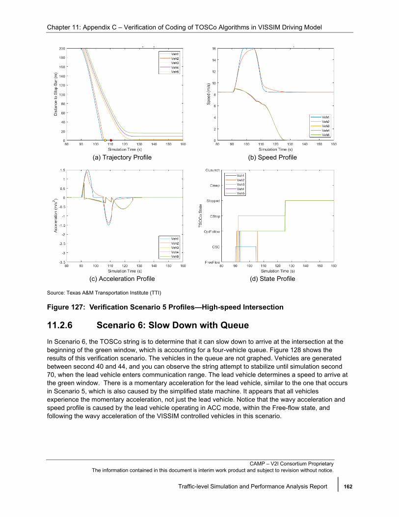
Chapter 11: Appendix C – Verification of Coding of TOSCo Algorithms in VISSIM Driving Model
CAMP – V2I Consortium Proprietary The information contained in this document is interim work product and subject to revision without notice.
Traffic-level Simulation and Performance Analysis Report | 162
(a) Trajectory Profile (b) Speed Profile
(c) Acceleration Profile (d) State Profile
Source: Texas A&M Transportation Institute (TTI)
Figure 127: Verification Scenario 5 Profiles—High-speed Intersection
11.2.6 Scenario 6: Slow Down with Queue In Scenario 6, the TOSCo string is to determine that it can slow down to arrive at the intersection at the beginning of the green window, which is accounting for a four-vehicle queue. Figure 128 shows the results of this verification scenario. The vehicles in the queue are not graphed. Vehicles are generated between second 40 and 44, and you can observe the string attempt to stabilize until simulation second 70, when the lead vehicle enters communication range. The lead vehicle determines a speed to arrive at the green window. There is a momentary acceleration for the lead vehicle, similar to the one that occurs in Scenario 5, which is also caused by the simplified state machine. It appears that all vehicles experience the momentary acceleration, not just the lead vehicle. Notice that the wavy acceleration and speed profile is caused by the lead vehicle operating in ACC mode, within the Free-flow state, and following the wavy acceleration of the VISSIM controlled vehicles in this scenario.

Chapter 11: Appendix C – Verification of Coding of TOSCo Algorithms in VISSIM Driving Model
CAMP – V2I Consortium Proprietary The information contained in this document is interim work product and subject to revision without notice.
Traffic-level Simulation and Performance Analysis Report | 163
(a) Trajectory Profile (b) Speed Profile
(c) Acceleration Profile (d) State Profile
Source: Texas A&M Transportation Institute (TTI)
Figure 128: Verification Scenario 6 Profiles—High-speed Intersection
11.2.7 Scenario 7: Stop with Queue In Scenario 7, the TOSCo string comes to a stop behind a four-vehicle string. The lead TOSCo vehicle enters communication range at about simulation second 36. Figure 129 shows the results of this verification scenario. The lead TOSCo vehicle enters a Coordinated Stop model immediately. The TTI Infrastructure algorithm changes the green window based on the current queue information, which impacts the behavior of this verification by causing the lead vehicle to re-plan the stop trajectory at about simulation second 42 and 50. At simulation second 42 and 50 the acceleration for the lead vehicle returns to zero and the speed profile becomes flat for a timestep. These adjustments are caused by the third and fourth vehicle in the queue being detected as queued at the intersection and the green window updating. When the queue cleared, after the signal changed green, the TOSCo string performed a coordinated launch.

Chapter 11: Appendix C – Verification of Coding of TOSCo Algorithms in VISSIM Driving Model
CAMP – V2I Consortium Proprietary The information contained in this document is interim work product and subject to revision without notice.
Traffic-level Simulation and Performance Analysis Report | 164
(a) Trajectory Profile (b) Speed Profile
(c) Acceleration Profile (d) State Profile
Source: Texas A&M Transportation Institute (TTI)
Figure 129: Verification Scenario 7 Profiles—High-speed Intersection

CAMP – V2I Consortium Proprietary The information contained in this document is interim work product and subject to revision without notice.
Traffic-level Simulation and Performance Analysis Report | 165
12 List of Acronyms
API Application Program Interface
ACC Adaptive Cruise Control
ASC/3 Advanced Signal Controller/3 version
BSM Basic Safety Message
CACC Cooperative Adaptive Cruise Control
CAMP Crash Avoidance Metric Partners LLC
CV Connected Vehicle
DLL Dynamic Link Library
DSRC Dedicated Short-Range Communication
EB Eastbound
FHWA Federal Highway Administration
GEH Value Geoffrey E. Havers Value
GHG Greenhouse Gases
GID Intersection Geometry Data
HCM Highway Capacity Manual
HV Host Vehicle
IDM Intelligent Driver Model
IOO Infrastructure Owner Operator
ITS JPO Intelligent Transportation Systems Joint Program Office
MOVES Motor Vehicle Emission Simulator
NDD Naturalistic Driving Data
OpMode Operating Mode
RMSE Root Mean Square Error
RSM Road Safety Message
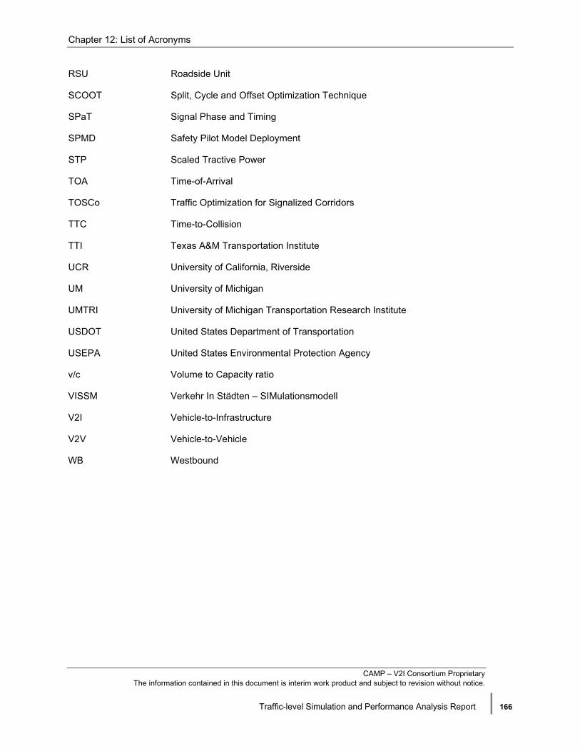
Chapter 12: List of Acronyms
CAMP – V2I Consortium Proprietary The information contained in this document is interim work product and subject to revision without notice.
Traffic-level Simulation and Performance Analysis Report | 166
RSU Roadside Unit
SCOOT Split, Cycle and Offset Optimization Technique
SPaT Signal Phase and Timing
SPMD Safety Pilot Model Deployment
STP Scaled Tractive Power
TOA Time-of-Arrival
TOSCo Traffic Optimization for Signalized Corridors
TTC Time-to-Collision
TTI Texas A&M Transportation Institute
UCR University of California, Riverside
UM University of Michigan
UMTRI University of Michigan Transportation Research Institute
USDOT United States Department of Transportation
USEPA United States Environmental Protection Agency
v/c Volume to Capacity ratio
VISSM Verkehr In Städten – SIMulationsmodell
V2I Vehicle-to-Infrastructure
V2V Vehicle-to-Vehicle
WB Westbound