Traffic Management System Performance Using … · Traffic Management System Performance Using...
44
CALIFORNIA PATH PROGRAM INSTITUTE OF TRANSPORTATION STUDIES UNIVERSITY OF CALIFORNIA, BERKELEY This work was performed as part of the California PATH Program of the University of California, in cooperation with the State of California Business, Transportation, and Housing Agency, Department of Trans- portation, and the United States Department Transportation, Federal Highway Administration. The contents of this report reflect the views of the authors who are responsible for the facts and the accuracy of the data presented herein. The contents do not necessarily reflect the official views or policies of the State of California. This report does not constitute a standard, spec- ification, or regulation. ISSN 1055-1417 March 2006 Traffic Management System Performance Using Regression Analysis California PATH Working Paper UCB-ITS-PWP-2006-3 CALIFORNIA PARTNERS FOR ADVANCED TRANSIT AND HIGHWAYS David Levinson, Wei Chen University of Minnesota Report for Task Order 4132
Transcript of Traffic Management System Performance Using … · Traffic Management System Performance Using...

CALIFORNIA PATH PROGRAMINSTITUTE OF TRANSPORTATION STUDIESUNIVERSITY OF CALIFORNIA, BERKELEY
This work was performed as part of the California PATH Program of the University of California, in cooperation with the State of California Business, Transportation, and Housing Agency, Department of Trans-portation, and the United States Department Transportation, Federal Highway Administration.
The contents of this report reflect the views of the authors who are responsible for the facts and the accuracy of the data presented herein. The contents do not necessarily reflect the official views or policies of the State of California. This report does not constitute a standard, spec-ification, or regulation.
ISSN 1055-1417
March 2006
Traffic Management System Performance Using Regression Analysis
California PATH Working PaperUCB-ITS-PWP-2006-3
CALIFORNIA PARTNERS FOR ADVANCED TRANSIT AND HIGHWAYS
David Levinson, Wei ChenUniversity of Minnesota
Report for Task Order 4132

Traffic Management System Performance
Using Regression Analysis A case study of Mn/DOT’s Traffic Management Systems
David Levinson1 Wei Chen2
Department of Civil Engineering University of Minnesota 500 Pillsbury Drive SE Minneapolis, MN 55455 [email protected] V: 612-625-6354 F: 612-626-7750 1. Associate Professor, 2. Research Assistant
Abstract
This study can be viewed as a preliminary exploration of using regression analysis to evaluate long-run
traffic management system performance. Four main traffic management systems in the Twin Cities metro
area --- Ramp Metering System, Variable Message Signs (VMS), Highway Helper Program, and High
Occupancy Vehicle (HOV) System were evaluated based on multiple regression models. Link speed and
incident rate were employed as the response variable separately. Consequently, regression analysis can be
a simple and effective research method for testing the macroscopic association between traffic
management and traffic system performance; however, additional research is still necessary to obtain an
overall evaluation of each of the traffic management systems. Furthermore, improvements could be made
through model improvement, adding relevant predictor variables, and decreasing data-limitations.
Key Words: Regression analysis; Traffic management system; Traffic system performance; Before-and-
after study; Response variables; Predictor variables; Multiple regression model; Speed; Incident Rate;
Ramp Metering System; Variable Message Signs (VMS); Highway Helper Program; High Occupancy
Vehicle (HOV) System.


Traffic Management System Performance Using Regression Analysis
1
Figure 1 : Ramp meter
1. INTRODUCTION
The Minnesota Department of Transportation (Mn/DOT) Traffic Management Center (TMC) started in
1972 to centrally control the freeway system in the Twin Cities metro area. The TMC aims to provide
motorists with a faster, safer trip on metro area freeways by optimizing the use of available freeway
capacity, efficiently managing incidents and special events, providing traveler information, and providing
incentives for ride sharing. The TMC realizes its goal through traffic management systems (TMS),
including Ramp Metering System, Variable Message Signs (VMS), Highway Helper Program, High
Occupancy Vehicle (HOV) System, Loop Detector System, Closed Circuit TV (CCTV) cameras, and
Traveler Information Program.
While the TMC has a long history of operation, the effectiveness of some of the traffic management
systems have been recently questioned---do they really help realize the objectives of the TMC, or rather,
do they make traffic conditions even worse? This study intends to evaluate the system-wide performance
of four main traffic management systems in the Twin Cities metro area --- Ramp Metering System,
Variable Message Signs, Highway Helper Program, and High Occupancy Vehicle (HOV) System using
regression analysis. The traditional before-and-after study and the regression analysis method were
compared, the outline of the regression analysis was presented and its limitations were stated. In the two
case studies, link speed and incident rate were employed as the response variable separately. Freeway
loop detector data and incident record by TMC freeway cameras were used for this study.
2. Main Traffic Management Systems This study evaluated the system-wide performance of four main traffic management systems in the Twin
Cities metro area --- Ramp Metering System, Variable Message Signs, Highway Helper Program, and
High Occupancy Vehicle (HOV) System. The objective, history, scope and
operation strategy of each system are summarized as follows [11, 12]:
I. Ramp Metering System Objective: Ramp meters in the Twin Cities are intended to reduce delay and
congestion, reduce accident rates, and smooth flow at on-ramp junctions by
helping merge traffic onto freeways and manage the flow of traffic through
bottlenecks.
History: The Minnesota Department of Transportation (Mn/DOT) first tested
ramp meters in 1969. There were approximately 427 ramp meters located

Traffic Management System Performance Using Regression Analysis
2
Figure 3 : Variable message signs
throughout the metro area freeway system with 416 of them centrally controlled (on-line), and 11 isolated
(stand-alone/pre-timed) meters by July 2000. The number of ramp meters in each year is shown in graph
1.
Scope: Currently, ramp meters manage access to approximately 210 miles of freeways in the Twin Cities
metro area. It covers all the freeways within the I-494/I-694 beltline and most of the freeways on and
outside the I-494/I-694 beltline.
Operation strategy: Ramp Metering System operates during peak traffic periods or when traffic or
weather conditions warrant their use. The original metering strategies (before October 16, 2000) were up
to four hours in the morning and up to five hours in the afternoon. Start and end times were determined
by corridor traffic conditions.
0
100
200
300
400
500
600
1970
1972
1974
1976
1978
1980
1982
1984
1986
1988
1990
1992
1994
1996
1998
2000
Year
Ramp Meters (Nos.)
Ramp Meters
Figure 2 : Number of Ramp Meters in Minnesota
II. Variable Message Signs Objective: Variable message signs are
devices installed along the roadside to display
messages of special events warning such as
congestion, incident, roadwork zone or speed
limit on a specific highway segment. These
messages alert travelers to traffic problems
ahead and help prevent secondary crashes.
History: There were 62 VMSs in operation
including both amber LED and rotary display type
signs by January 2001. The start-up dates of
VMSs generally coincided with the start-up dates of the on-line metering in that same freeway segment.
Scope: About 50 of the 62 VMSs are located within (and on) the I-494/I-694 beltline.
Operation strategy: Instant messages are provided to alert travelers to traffic problems ahead.
Traffic Management System Performance Using Regression Analysis
3
III. Highway Helper Program Objective: Highway helper program intends to minimize congestion through the quick removal of stalled
vehicles from the freeway, reduce the number of secondary accidents, assist stranded motorists and aid
the State Patrol with incident management. It plays a major role in incident management in the Twin
Cities metro area.
History: Highway Helper program was initiated in December 1987, and additional miles were added in
September, 1996. Currently there are 8 highway helper routes.
Scope: Highway helper program patrols eight routes (170 miles) in the Twin Cities metro area.
Operation strategy: From 5:00 AM to 7:30 PM Monday through Friday, limited hours on weekends.
IV. High Occupancy Vehicle (HOV) System Objective: The purpose of the HOV System is to move more people in fewer vehicles and provide a
quicker, more reliable trip for those who rideshare or take the bus. A HOV is a vehicle with two or more
people in it. Vanpools, car-pools, buses and motorcycles are classified as HOVs.
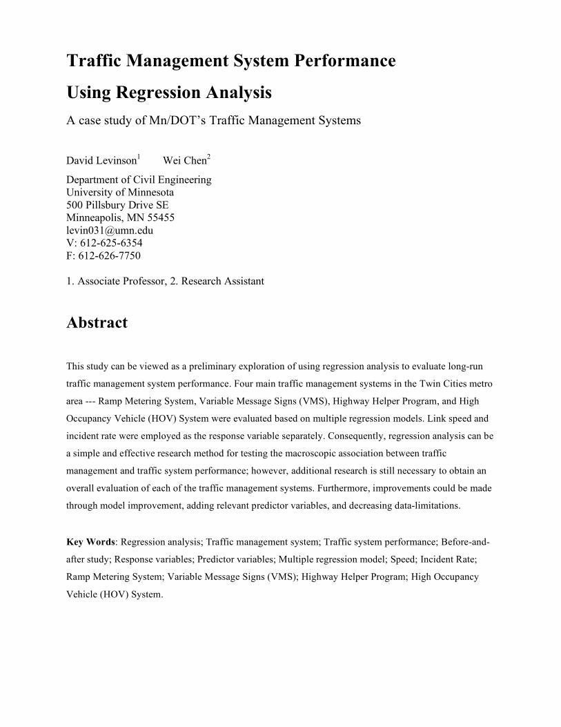
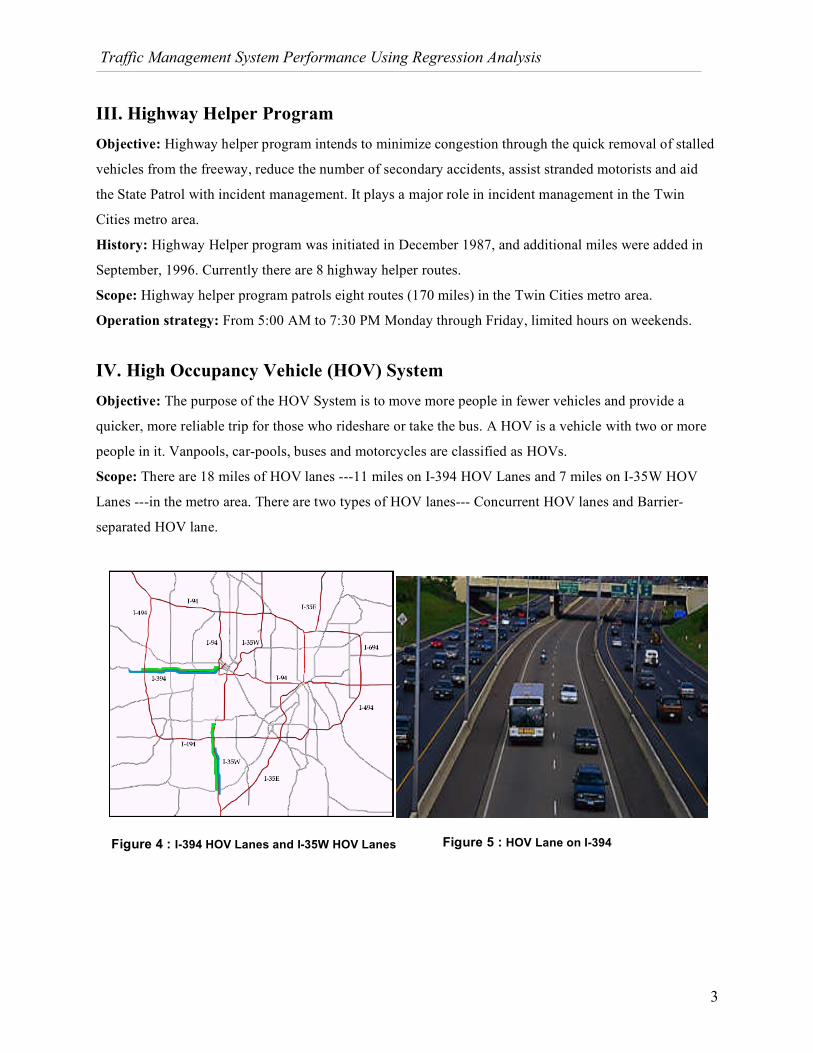
Scope: There are 18 miles of HOV lanes ---11 miles on I-394 HOV Lanes and 7 miles on I-35W HOV
Lanes ---in the metro area. There are two types of HOV lanes--- Concurrent HOV lanes and Barrier-
separated HOV lane.
Figure 5 : HOV Lane on I-394 Figure 4 : I-394 HOV Lanes and I-35W HOV Lanes
Traffic Management System Performance Using Regression Analysis
4
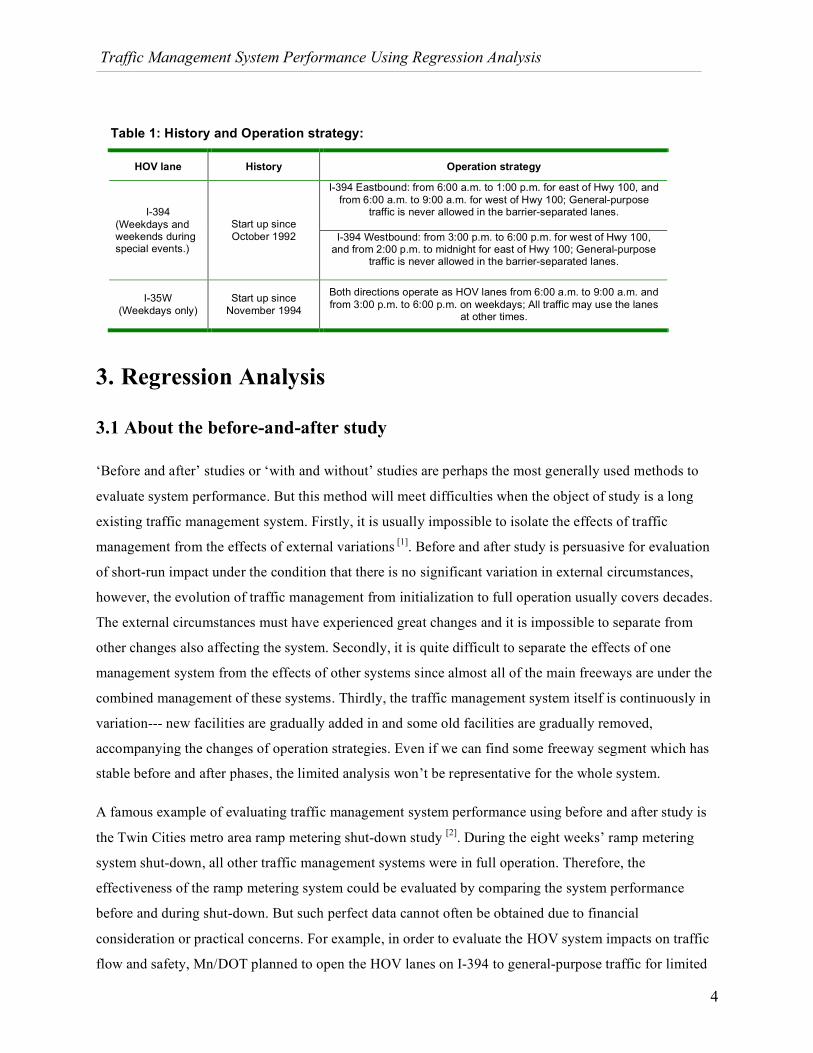
Table 1: History and Operation strategy:
HOV lane History Operation strategy
I-394 Eastbound: from 6:00 a.m. to 1:00 p.m. for east of Hwy 100, and from 6:00 a.m. to 9:00 a.m. for west of Hwy 100; General-purpose
traffic is never allowed in the barrier-separated lanes.
I-394 (Weekdays and weekends during special events.)
Start up since October 1992 I-394 Westbound: from 3:00 p.m. to 6:00 p.m. for west of Hwy 100,
and from 2:00 p.m. to midnight for east of Hwy 100; General-purpose traffic is never allowed in the barrier-separated lanes.
I-35W (Weekdays only)
Start up since November 1994
Both directions operate as HOV lanes from 6:00 a.m. to 9:00 a.m. and from 3:00 p.m. to 6:00 p.m. on weekdays; All traffic may use the lanes
at other times.
3. Regression Analysis
3.1 About the before-and-after study
‘Before and after’ studies or ‘with and without’ studies are perhaps the most generally used methods to
evaluate system performance. But this method will meet difficulties when the object of study is a long
existing traffic management system. Firstly, it is usually impossible to isolate the effects of traffic
management from the effects of external variations [1]. Before and after study is persuasive for evaluation
of short-run impact under the condition that there is no significant variation in external circumstances,
however, the evolution of traffic management from initialization to full operation usually covers decades.
The external circumstances must have experienced great changes and it is impossible to separate from
other changes also affecting the system. Secondly, it is quite difficult to separate the effects of one
management system from the effects of other systems since almost all of the main freeways are under the
combined management of these systems. Thirdly, the traffic management system itself is continuously in
variation--- new facilities are gradually added in and some old facilities are gradually removed,
accompanying the changes of operation strategies. Even if we can find some freeway segment which has
stable before and after phases, the limited analysis won’t be representative for the whole system.
A famous example of evaluating traffic management system performance using before and after study is
the Twin Cities metro area ramp metering shut-down study [2]. During the eight weeks’ ramp metering
system shut-down, all other traffic management systems were in full operation. Therefore, the
effectiveness of the ramp metering system could be evaluated by comparing the system performance
before and during shut-down. But such perfect data cannot often be obtained due to financial
consideration or practical concerns. For example, in order to evaluate the HOV system impacts on traffic
flow and safety, Mn/DOT planned to open the HOV lanes on I-394 to general-purpose traffic for limited

Traffic Management System Performance Using Regression Analysis
5
period in 2001 for the before and after data collection. However, this plan was barred by FHWA due to
policy considerations.
The performance evaluation of traffic management system can provide important information for
planning and for the rationalization of operating budget allocations. We hope to explore a simple and
effective approach for this task. Regression analysis is promising. Comparing with before and after study,
regression analysis doesn’t try to design the stable external circumstances and isolate the effects of the
object in study from the effects of combining factors. In fact, it is often quite difficult or even impossible
to design or seek the ‘stable’ external circumstances in a dynamic traffic system. For example, when we
evaluate effects of traffic management systems on incident rate, we need to use several years’ data to get
large enough sample, in this case, it is meaningless to assume unvaried external circumstances [1].
Regression analysis is different from before and after study in that it tries to search out all the potential
elements (including traffic management) that effect system performance, record their variation and use
these elements as the regression predictor variables to test the association between traffic system
performance and traffic management.
3.2 Define the response variable of the regression model
Performance measurement proceeds by identifying and quantifying some feature of the performance of
the traffic system (such as travel time or accident rate) and using this to infer the performance of some
part of the traffic management system [1]. In regression analysis, the measure of traffic system
performance will be employed as the response variable, the traffic management systems will be included
in the predictor variables, and their performance will be inferred by their associations with the response
variable and by comparison with the coefficients of related predictor variables.
There can be many performance measures of the traffic system [10]. However, a measure can be used as
the response variable only if it is significantly associated with the operation objectives of the traffic
management systems; furthermore, it should be straightforward to identify the relevant predictor
variables.
Speed and incident rate meet these criteria and will be used as the response variables in the
following regression analysis. The reason for using speed instead of travel time is that the
regression model will include observations from different corridor segments, travel time will
present no more information than speed, but it will be influenced by the differences in length of
the corridor segments. Actually, some related measures, such as travel time, delays, and travel
time reliability, could be derived directly from speed. Some other measures, including
environmental impacts and fuel consumption, could also be derived from speed by combining
with other factors such as volume, vehicle types, and gasoline quality.
Traffic Management System Performance Using Regression Analysis
6
3.3 The framework of an ideal regression model
An ideal regression model is a multiple regression model which employs all the relevant elements
affecting system performance as its explanatory variables. The relevant elements can be classified into the
following four categories:
1. Infrastructure characteristics, which include capacity, geometric structure, pavement quality and
conditions, geographic characteristics and construction activity impact. Capacity has significant effects on
speed, but detailed information of capacity is difficult to obtain for each freeway segment. In this case, the
number of lanes of the freeway segment could be used as the indication of capacity if the corridors in
study are in the same grade-level, e.g., all are interstate freeways. Geometric structure includes the
elements of horizontal and vertical curvature, sight distance and the distance between entrance and exit in
the same segment. Pavement quality can be good, normal, and poor; pavement conditions can be dry, wet,
or snow covered [2]. The geographic characteristics of freeways in the Twin Cities metro area can be
classified into four groups: the I-494/I-694 beltline freeway, intercity connector, radial freeway within the
I-494/I-694 beltline, and radial freeway outside the beltline [2].
2. Traffic characteristics, which include traffic volume, density, vehicle fleet composition, and level of
service. Vehicle fleet composition includes passenger car and freight truck, heavy truck fleet has
significant impact on freeway capacity and speed.
3. Traffic Management Strategies, which include Ramp Metering System, Variable Message Signs,
Highway Helper Program, High Occupancy Vehicle (HOV) System, and some other traffic management
strategies such as Traveler Information Program.
4. Other factors, which include traffic incident impact and weather impact.
Figure 6 shows the framework of the ideal regression model.
3.4 Limitations of Regression analysis
When before and after is impossible or too costly, regression analysis can be a good substitute. But
regression analysis can’t obtain all the information we need to know about the traffic management
system. For example, regression analysis just tells us the association between ramp metering and system
mainline speed, it can’t tell us whether the travel time saving caused by ramp metering system (if any) on
the mainline could offset ramp delay. It also can’t tell us whether the person-hours increase on general-
purpose lanes (if any) could be offset by the person-hours decrease on HOV lanes. Consequently,
regression analysis can be a simple and effective research method for testing the macroscopic association
or trend between traffic management and traffic system performance; however, to obtain an overall
evaluation of each of the traffic management systems, additional research is still necessary.

Traffic Management System Performance Using Regression Analysis
7
Figure 6 : The framework of an ideal regression model
Speed or Incident Rate
Response Variable
Predictor Variables
Pavement quality & conditions Geographic characteristics
Geometric structure
Construction activity impact
Capacity
Level of service
Vehicle fleet composition
Traffic volume or density
Highway Helper Program High Occupancy Vehicle System
Variable Message Signs
Ramp Metering System
Other traffic management systems
Traffic Incident Impact (When using speed as response variable)
Weather Variations
Traffic Characteristics
Traffic Management Strategies
Other factors
Infrastructure Characteristics
Traffic Management System Performance Using Regression Analysis
8
4. Case study I : Using link speed as response variable 4.1 Regression Model 1. Predictor variables:
It should be mentioned firstly that due to the limitation of data, we are not able to test all the potential
predictor variables described in the ideal regression model, this is a deficiency of this case study.
For infrastructure characteristics, we used capacity (number of lanes); for traffic characteristics, we used
density; for traffic management strategies, we tested Ramp Metering System, Variable Message Signs,
Highway Helper Program, and High Occupancy Vehicle (HOV) System; and for other factors, we used
traffic incident impact.
We also added 22 corridor dummies, which classified the observations into 22 corridor groups. Each
group has its distinctive traffic, infrastructure, and spatial characteristics. The corridor dummy assigned to
each observation can be viewed as one ‘attribute’ just like the ‘number of lanes’. As an example,
comparing with I-494 NB & SB beltline corridors which carry traffic from suburb to suburb, I-94
intercity connectors cross major commercial zones and they have higher intersection density (or entrance
& exit density). Given the same mainline density, I-94 intercity connectors should be slower than I-494
NB & SB beltline freeways due to more entering and exiting disturbance. As another example, I-35W
corridors (south of I-494) have higher percentage of heavy commercial traffic than I-35E corridors (north
of I-94). Since heavy commercial flows have significant impacts on freeway capacity, holding other
conditions fixed, we would expect I-35W corridors to slower than I-35E corridors.
Finally, we don’t rule out the possibility that the addition of other predictor variables will change the
results.
2. Detect multicollinearity
Since we face a multiple regression problem, we should use the correlation matrix to detect the possible
multicollinearity. Multicollinearity is likely to exist between density and the TMS dummies. It is assumed
that multicollinearity will be diagnosed to be present if the absolute value of the correlation between two
predictor variables is larger than 0.6, otherwise no multicollinearity. From the correlation matrixes
(Appendix 3) we get to know that each correlation is less than 0.6, therefore, no multicollinearity
exists between density and the TMS dummies. What should be noted is the low correlation between ramp
metering and mainline density. In practice, people tend to inflate the correlation between ramp metering
and mainline density. It is often thought to be true that a segment controlled by ramp metering will have

Traffic Management System Performance Using Regression Analysis
9
relatively lower density than a segment without metering. But actually obvious linear relationship
between ramp metering and mainline density can’t be found from our data. The reason should be that
density is such a complex measurement which is associated with many factors, and ramp metering is just
one of them.
On the other hand, ramp metering affects mainline speed through not only mainline density but also other
traffic factors such as drivers’ behaviors. When ramp cars try to merge into the mainline, mainline drivers
usually have to slow down or even turn aside to let them in. That is, ramp cars will have impacts to
mainline drivers’ behaviors even if their merging doesn’t cause significant increase in mainline density.
(To get an intuitive understanding about this just think that even when the middle lane has the same
density as the right lane, the middle lane is typically faster than right lane because the right lane has to
sustain the impacts of merging(and exiting) cars). Under ramp metering control, ramp cars enter the
freeway in a spaced and controlled manner. Even in the case that ramp metering doesn’t significantly
decrease mainline density, its effects in controlling merging disruption to mainline traffic will lead to
mainline speed increase.
3. Model expression
Model 1. Incident-free case
Hourly average speed = ß0 + ß D× Density + ß TMT1× Ramp Meter (1,0) + ß TMT2× VMS (1,0) + ß TMT3×
Concurrent HOV (1,0) + ß TMT4× Barrier-separated HOV (1,0) + ß L1× Two-Lane (1,0) + ß L2× Three-Lane
(1,0) + ß L3× Four-Lane (1,0) + ßC1~C22× Corridor dummies+ ε
Where,
ß D indicates the coefficient of hourly average density;
ß TMT1~ TMT4 indicate the coefficients of Ramp Meter Dummy, VMS Dummy, Concurrent HOV Dummy,
and Barrier-separated HOV Dummy;
ß L1~ L3 indicate the coefficients of the number of lanes-- two-Lane, three-Lane, and four-Lane;
ßC1~C22indicate the coefficients of the 22 corridors we selected for this study (refer to 4.3 Corridor
selection and study periods).
Model 2. Incident case
Hourly average speed = ß0 + ßD× Density + ßTMT1× Ramp Meter (1,0) + ßTMT2× VMS (1,0) + ßTMT3×
Highway Helper Program (1,0) + ßTMT4× Concurrent HOV (1,0) + ßTMT5× Barrier-separated HOV (1,0) +
ßL1×Two-Lane (1,0) + ßL2× Three-Lane (1,0) + ßL3× Four-Lane (1,0) + ßI1~I5× Incident* + ßC1~C22×
Corridor dummies + ε
Traffic Management System Performance Using Regression Analysis
10
Where,
ßI1~I5 indicate the coefficients of the five incident groups; Incident* indicates the following five groups:
Incident1 --the incident occurred within the studied segment;
Incident2 --the incident occurred in the first segment upstream the studied segment;
Incident3 --the incident occurred in the second segment upstream the studied segment;
Incident4 --the incident occurred in the first segment downstream the studied segment;
Incident5 --the incident occurred in the second segment downstream the studied segment;
Notes:
1. Highway Helper Program is not included in the incident-free case because when the studied segments
are incident-free, Highway Helper Program has no effects to the segments;
2. Ramp Metering Dummy, Highway Helper Dummy, VMS Dummy, Concurrent HOV Dummy, and
Barrier-separated HOV Dummy are defined as follows:
Ramp Meter=1 if the segment is under ramp metering control; otherwise, Ramp Meter=0.
VMS=1 if the segment is within the impacting range of VMS; otherwise, VMS=0.
Highway Helper =1 if the segment is within highway helper program patrol area; otherwise, Highway
Helper =0.
HOV=1 if the corridor has HOV lane(s) in operation; otherwise, HOV=0.
4.2 Measure speed and density using loop detector data
1. Measuring speed in one hour’s interval
Loop detectors provide freeway volume and occupancy information in 30-second intervals. The data-
extracting program Data_Extraction TMC, which is developed by MN/DOT TMC, was used for
extracting and formatting freeway loop detectors data. Volume Qi and occupancy Ki in 5-minute intervals
were extracted using this program.
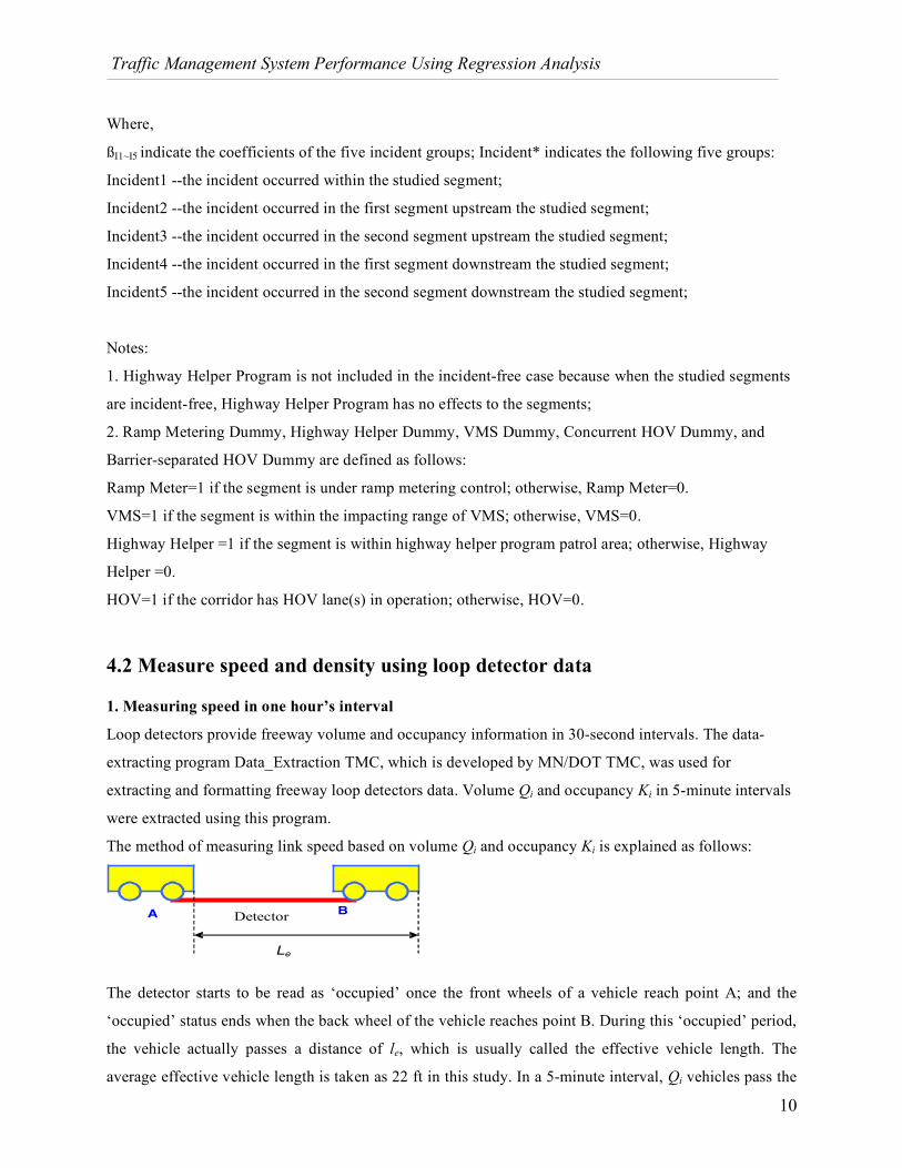
The method of measuring link speed based on volume Qi and occupancy Ki is explained as follows:
Le
Detector A B
The detector starts to be read as ‘occupied’ once the front wheels of a vehicle reach point A; and the
‘occupied’ status ends when the back wheel of the vehicle reaches point B. During this ‘occupied’ period,
the vehicle actually passes a distance of le, which is usually called the effective vehicle length. The
average effective vehicle length is taken as 22 ft in this study. In a 5-minute interval, Qi vehicles pass the
Traffic Management System Performance Using Regression Analysis
11
detector, therefore, the total distance driven by these Qi vehicles should be Qi × le/5280 (mile).
Furthermore, the detector is occupied for Ki (%) percent of 5 minutes’ time, that means the total time
actually used for traveling in a 5-minute interval should be 300×Ki /100 (sec). Therefore we can obtain the
space mean speed usduring a 5-minute interval as follows [5]:
!
us =total distance
total time =
3600 "100 "Qi " le
5280 " 300 "Ki
(mile/hr) (1)
Where:
us Space mean speed of one detector in 5-minute intervals (mile/hr);
le Effective vehicle length (ft);
Qi and Ki Volume and occupancy of one detector in 5-minute intervals
us is the space mean speed for one lane in 5-minute intervals. Freeway segments have 2 to 5 lanes. Space
mean speed for one segment is estimated using the weighted mean speed (weighted by volume) of all
lanes. The space mean speed for a three-lane segment is as follows:
us,Q=Q1us ,Q1 + Q2
us,Q2 + Q3us,Q3
Q1+ Q
2+Q
3
(2)
Space mean speed for one segment in one hour’s interval is the arithmetic mean of the twelve 5-minute
speeds of this segment in one hour.
It should be noted that when the loop detectors read to be ‘0’ for occupancy, the calculated speed will
have invalid number and the observation will be removed. Loop detectors read ‘0’ for occupancy in two
conditions: 1. Loop detectors malfunction; 2. It happens to have no vehicles passing by during the
counting period. Under condition 1, the occupancy will continue to be 0 for several hours or even days;
under condition 2, the occupancy will be 0 for at least 5 minutes (because the volume and occupancy data
were extracted in 5-minute intervals in this study.). When condition 2 happens, the observations with
relatively low average hourly speeds are removed. This might lead to some bias in the regression result.
But since the four hours in study (7:00AM—8:00AM, 8:00AM—9:00AM, 4:00PM—5:00PM and
5:00PM—6:00PM) are all peak hours, condition 2 happens with quite low probability, and its influence
on the final result will be slight.
2. Measuring density in one hour’s interval
The equation 1 can be rewritten as follows:
us =100 !Q ! le
5280 ! 300 ! occupancy=
Q
300!
le
5280occupancy
100
=
q !le
5280occupancy
100
(mile / s) (3)
Traffic Management System Performance Using Regression Analysis
12
then, density can be calculated as follows:
k =q
us
=q
q !le
5280occupancy
100
=
occupancy
100le
5280
(veh / mile) (4)
Effective vehicle length le is assumed to be 22 feet, and the density k will be equal to:
k =
occupancy
10022
5280
=5280
100 ! 22! occupancy = 2.4 ! occupancy(veh /mile) (5)
The density k estimated using equation 5 is the average density for one lane in 5-minute intervals. The
average density of one segment is the arithmetic mean of the densities of all lanes. Furthermore, the
average density of one segment in one hour’s interval is the arithmetic mean of the twelve 5-minute
densities of this segment in one hour. The unit of segment density is vehicles per mile, per lane.
4.3 Corridor selection and study periods
1. Corridor selection
Totally 22 corridors were selected for this study based on the following two rules:
I. The selected corridors should form a geographically representative sample of the entire system.
Based on the geographic characteristics, the freeway corridors within the Twin Cities metro area
can be classified into the following four types: the I-494/I-694 beltline freeway, intercity
connector, radial freeway within the I-494/I-694 beltline, and radial freeway outside the beltline [2]. The 22 selected corridors covered these four types (refer to Appendix 1 and 2 ).
II. The selected corridors should include segments with and without ramp meters, with and without
VMS, with and without highway helper program, and with and without HOV lanes (refer to Table
2).
2. Study periods
Study periods range from 1998 to 2000, which includes the periods before ramp meter start-up, ramp
meter in full operation, and ramp meter eight weeks’ shut-down in 2000; before VMS start-up and VMS
in full operation; highway helper program in full operation; and HOV system in full operation.
It is noted that no ‘before’ data are included for highway helper program and HOV system. The reason is
that the start-up dates of I–394 HOV lanes and I-35W HOV lanes are in 1992 and 1994 respectively, but
no loop detector data are available before 1994. As to the highway helper program, the initial patrol

Traffic Management System Performance Using Regression Analysis
13
routes started in December 1987, and additional routes were added from September, 1996, the ‘before’
data could be obtained for the additional routes. However, although loop detector data were available
from 1994, they were insufficient before 1996. Furthermore, three years already form a long study period.
The longer the period, the more variations and fluctuations experienced in the network, which will
significantly affect the regression result. Consequently, we didn’t include the before data of the additional
routes of highway helper program in the database. The study periods and corridor selection are
summarized in Table 2: Table 2 : Corridor selection and study periods
Ramp Meter VMS Highway Helper program HOV lanes
Corridor Selection
Corridors with Ramp Meters (RM=1); Corridors without Ramp Meters (RM=0);
Corridors with VMS (VMS=1); Corridors without VMS (VMS=0);
Corridors with Highway Helper (Highway Helper=1); Corridors without Highway Helper (Highway Helper=0);
Corridors with HOV lanes (HOV=1); Corridors without HOV lanes (HOV=0);
Study periods
Before RM start-up (RM=0); RM in full operation (RM=1); RM eight weeks’ shut-down in 2000 (RM=0);
Before VMS start-up (VMS=0); VMS in full operation (VMS=1);
Highway Helper Program in full operation (Highway Helper=1);
HOV lanes in full operation (HOV=1);
In addition, the following criteria are applied for data collection:
1. Samples are gathered on typical workdays (Tuesday, Wednesday, and Thursday). Monday and
Friday are avoided;
2. Holidays are avoided;
3. A gap between the "before-after" periods is taken to permit the public to become accustomed to
the new improvement before a check on its effect is begun [8]. The length of gaps range from 30
to 80 days in 1999. Due to the limited normal loop detector data, the length of gaps in 1998 range
from 10 to 20 days.
4.4 Results and analysis: The statistical software STATA was used for the study. Results were obtained for four peak hours --
7:00AM—8:00AM, 8:00AM—9:00AM, 4:00PM—5:00PM, and 5:00PM—6:00PM under both incident-
free and incident cases. All the traffic management systems are in operation in these four hours. The
regression results are summarized in Table 3. Note: detailed regression results of case study I are in
Appendix 6-13.
Traffic Management System Performance Using Regression Analysis
14
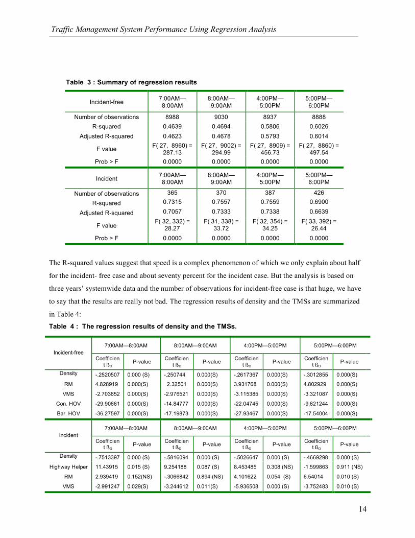
Table 3 : Summary of regression results
Incident-free 7:00AM—8:00AM
8:00AM—9:00AM
4:00PM—5:00PM
5:00PM—6:00PM
Number of observations 8988 9030 8937 8888 R-squared 0.4639 0.4694 0.5806 0.6026
Adjusted R-squared 0.4623 0.4678 0.5793 0.6014
F value F( 27, 8960) = 287.13
F( 27, 9002) = 294.99
F( 27, 8909) = 456.73
F( 27, 8860) = 497.54
Prob > F 0.0000 0.0000 0.0000 0.0000
Incident 7:00AM—8:00AM
8:00AM—9:00AM
4:00PM—5:00PM
5:00PM—6:00PM
Number of observations 365
370
387
426 R-squared 0.7315
0.7557
0.7559
0.6900
Adjusted R-squared 0.7057
0.7333
0.7338
0.6639
F value
F( 32, 332) = 28.27
F( 31, 338) = 33.72
F( 32, 354) = 34.25
F( 33, 392) = 26.44
Prob > F 0.0000 0.0000 0.0000 0.0000
The R-squared values suggest that speed is a complex phenomenon of which we only explain about half
for the incident- free case and about seventy percent for the incident case. But the analysis is based on
three years’ systemwide data and the number of observations for incident-free case is that huge, we have
to say that the results are really not bad. The regression results of density and the TMSs are summarized
in Table 4: Table 4 : The regression results of density and the TMSs.
7:00AM—8:00AM 8:00AM—9:00AM 4:00PM—5:00PM 5:00PM—6:00PM Incident-free
Coefficient ßD P-value Coefficien
t ßD P-value Coefficient ßD P-value Coefficien
t ßD P-value
Density
-.2520507 0.000 (S) -.250744 0.000(S) -.2617367 0.000(S) -.3012855 0.000(S)
RM 4.828919 0.000(S) 2.32501 0.000(S) 3.931768 0.000(S) 4.802929 0.000(S)
VMS -2.703652 0.000(S) -2.976521 0.000(S) -3.115385 0.000(S) -3.321087 0.000(S)
Con. HOV -29.90661 0.000(S) -14.84777 0.000(S) -22.04745 0.000(S) -9.621244 0.000(S)
Bar. HOV -36.27597 0.000(S) -17.19873 0.000(S) -27.93467 0.000(S) -17.54004 0.000(S)
7:00AM—8:00AM 8:00AM—9:00AM 4:00PM—5:00PM 5:00PM—6:00PM Incident
Coefficient ßD P-value Coefficien
t ßD P-value Coefficient ßD P-value Coefficien
t ßD P-value
Density
-.7513397 0.000 (S) -.5816094 0.000 (S) -.5026647 0.000 (S) -.4669298 0.000 (S)
Highway Helper 11.43915 0.015 (S) 9.254188 0.087 (S) 8.453485 0.308 (NS) -1.599863 0.911 (NS)
RM 2.939419 0.152(NS) -.3066842 0.894 (NS) 4.101622 0.054 (S) 6.54014 0.010 (S)
VMS -2.991247 0.029(S) -3.244612 0.011(S) -5.936508 0.000 (S) -3.752483 0.010 (S)
Traffic Management System Performance Using Regression Analysis
15
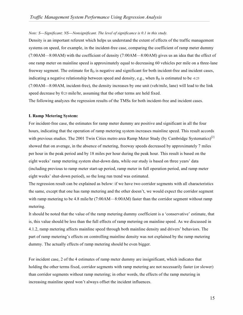
Note: S---Significant; NS---Nonsignificant. The level of significance is 0.1 in this study.
Density is an important referent which helps us understand the extent of effects of the traffic management
systems on speed, for example, in the incident-free case, comparing the coefficient of ramp meter dummy
(7:00AM—8:00AM) with the coefficient of density (7:00AM—8:00AM) gives us an idea that the effect of
one ramp meter on mainline speed is approximately equal to decreasing 60 vehicles per mile on a three-lane
freeway segment. The estimate for ßD is negative and significant for both incident-free and incident cases,
indicating a negative relationship between speed and density, e.g., when ßD is estimated to be -0.25
(7:00AM—8:00AM, incident-free), the density increases by one unit (veh/mile, lane) will lead to the link
speed decrease by 0.25 mile/hr, assuming that the other terms are held fixed.
The following analyzes the regression results of the TMSs for both incident-free and incident cases.
I. Ramp Metering System:
For incident-free case, the estimates for ramp meter dummy are positive and significant in all the four
hours, indicating that the operation of ramp metering system increases mainline speed. This result accords
with previous studies. The 2001 Twin Cities metro area Ramp Meter Study (by Cambridge Systematics)[2]
showed that on average, in the absence of metering, freeway speeds decreased by approximately 7 miles
per hour in the peak period and by 18 miles per hour during the peak hour. This result is based on the
eight weeks’ ramp metering system shut-down data, while our study is based on three years’ data
(including previous to ramp meter start-up period, ramp meter in full operation period, and ramp meter
eight weeks’ shut-down period), so the long run trend was estimated.
The regression result can be explained as below: if we have two corridor segments with all characteristics
the same, except that one has ramp metering and the other doesn’t, we would expect the corridor segment
with ramp metering to be 4.8 mile/hr (7:00AM—8:00AM) faster than the corridor segment without ramp
metering.
It should be noted that the value of the ramp metering dummy coefficient is a ‘conservative’ estimate, that
is, this value should be less than the full effects of ramp metering on mainline speed. As we discussed in
4.1.2, ramp metering affects mainline speed through both mainline density and drivers’ behaviors. The
part of ramp metering’s effects on controlling mainline density was not explained by the ramp metering
dummy. The actually effects of ramp metering should be even bigger.
For incident case, 2 of the 4 estimates of ramp meter dummy are insignificant, which indicates that
holding the other terms fixed, corridor segments with ramp metering are not necessarily faster (or slower)
than corridor segments without ramp metering; in other words, the effects of the ramp metering in
increasing mainline speed won’t always offset the incident influences.
Traffic Management System Performance Using Regression Analysis
16
II. Variable message signs:
It should be mentioned firstly that different from Ramp Metering system and HOV system, which both
have relatively fixed operational hours, VMS is active only when ‘special events’ happen. But it is
impossible for us to obtain the detailed starting time and duration of these VMS messages. Therefore, we
had to define the VMS dummy as ‘1’ if the studied corridor segment is within the impacting range of
VMS. The impacting range of VMS is defined as the segments that can ‘see’ the VMS messages and the
2 to 3 segments downstream the VMS. Therefore, what we estimate here is actually the association
between speed and VMS impacting range.
For both incident-free case and incident case, the estimates for VMS dummy are negative and significant
in all the four hours. The negative association between speed and VMS impacting range can be explained
as follows:
1. VMSs have impacts on drivers’ behaviors. VMSs are devices installed along the roadside to
display messages of special events warning such as congestion, incident, roadwork zone or speed
limit to alert travelers of traffic problems ahead. The messages displayed by VMSs have impacts
on drivers’ behaviors. Drivers typically slow down to view the message and to plan alternative
routes, and some of them may divert to other roadways.
2. The distribution characteristics of VMSs contribute to the negative association. Most of the
VMSs in the Twin Cities metro area are located at the freeway segments with high AADT. These
segments are typically more congested and have lower mainline speed. The negative relationship
between speed and variable message signs is partly due to the distribution characteristics of the
VMSs.
Then, should we stop using VMS since VMS impacting range is associated with lower mainline speed?
Probably not. Because the speed decrease at one corridor (VMS impacting range) may prevent terrible
congestion at some other corridors. Further study should be done to give a more comprehensive
evaluation of VMS.
III. Highway Helper program:
Highway Helper Program is not included in the incident-free case because when the studied segments are
incident-free, Highway Helper Program is not active.
In the incident case, two of the four estimates are positive and significant (7:00AM-8:00AM and
8:00AM-9:00AM), and two are insignificant (4:00PM-5:00PM and 5:00PM-6:00PM). The positive and
significant association between speed and highway helper program indicates that in incident case, the
corridor segments within highway helper patrol areas will be faster than the corridor segments out of the
areas; while the insignificant relationship can be due to two reasons:
1. the sample size is insufficient to detect the alternative in this situation [13] ;

Traffic Management System Performance Using Regression Analysis
17
2. It is partly due to the fact that the incident impact on speed is not in one direction. Although the
speed on corridors covered by highway helper program can be increased (if any), the speed on
corridors out of highway helper program won’t necessarily decrease. Actually, incidents
downstream the studied segment typically decrease its speed, while incidents upstream the
segment might cause increase in its speed.
IV. HOV system:
In the analysis of the two kinds of HOV systems, the speed is for the general-purpose lanes. That’s
because we have no interest to test the HOV lanes’ association with speed (they will have positive
relationship); what we want to estimate is the impact of the operation of HOV lanes to the general-
purpose lanes. The regression results in incident-free case show that all the 8 estimates (for both
Concurrent HOV dummy and Barrier-separated HOV dummy) are negative and significant, which
indicates that the operation of HOV lanes is associated with lower speed on the general-purpose lanes.
For incident case, it is difficult to give the regression results a reasonable explanation due to the low data-
quality. Incident log didn’t record on which lane the incidents actually happened---HOV lanes or general-
purpose lanes. So we didn’t list the HOV regression results for incident case.
5. Case study II : Using incident rate as response variable 5.1 Data collection TMC freeway incident record for Twin Cities metro area started from 1991, but we only used the data of
Fall 2000 for this study. The earlier years’ incident data can’t be used for this systemwide analysis due to
the following reasons:
1) The incident record started at different years for different corridors --- some corridors from 1991,
while some others even as late as 1998;
2) Based on the incident record, the incidents increased tremendously in the past ten years. But this
increase was partly caused by the addition of new cameras, the upgrade of equipment, and the
improved monitoring methods.
We collected the incident data for two periods in Fall 2000 --- 37 workdays (from Aug. 22 to Oct.
13)before ramp metering system shut-down (Refer to 2001 Twin Cities Metro Area Ramp Meter Study
Final report [2] ) and 37 workdays ( from Oct. 16 to Dec. 07) during ramp metering system shut-down.
Incident records during these two periods have much higher quality than before because during these two
periods the camera monitoring system covered the whole network and was operated under the same
monitoring strategies and equipment conditions. In addition, incident data was counted between 7:00AM
to19:00 PM, which were the operational hours of the traffic management system.

Traffic Management System Performance Using Regression Analysis
18
Figure 7. Intersections on Corridor 1
As to incident types, since what we want to test is the association of incident rate and the traffic
management system, we removed the incidents caused by vehicle mechanical malfunctions such as stalls
and vehicle fires and the incidents caused by debris on road. Finally three kinds of incidents were
included--- crash, rollover and spinout, where, crash incidents counted for more than 97% of all incidents.
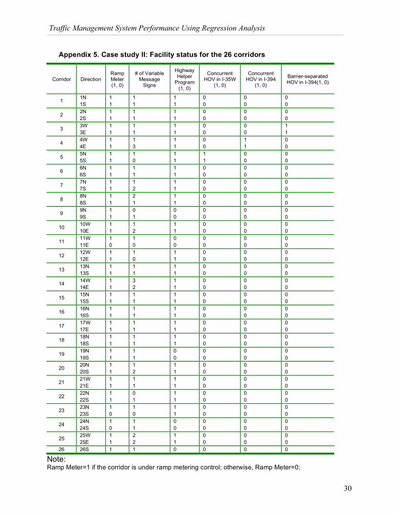
5.2 Corridor selection In total, 26 corridors were selected for this study which nearly cover the whole Twin Cities metro area
freeway network (refer to Appendix 4). The unselected corridors were those outside of TMC camera
monitoring. The facility status of each corridor was summarized in Appendix 5.
5.3 Regression model It should be noted that with the short incident counting periods (37 workdays before and during ramp
metering shut-down respectively) we can guarantee the quality of incident data; however, it is also due to
the short incident counting periods we have to select long corridors to ensure a non-zero number of
incidents. When the corridors are long, it is impossible to include some traffic or infrastructure
characteristics as predictor variables although these characteristics may be relevant to the response
variable. For example, some traffic stream characteristics -such as link speed, flow or density - should be
the potential predictor variables of incident regression analysis, but for a long corridor (which has several
segments), the speed, flow or density of the segments vary greatly and none of them could be represented
by a single value. Also the geometric characteristics can’t be represented by a
uniform format for all the segments of a long corridor. Finally we included limited
predictor variables in the regression model.
The multiple regression model can be represented as below:
Incident Rate =0
! +I
! × Intersection Density + R
! × Ramp Meter (1,0) + V! ×
VMS Density + H
! × Highway Helper Program (1,0) + 35!C" × Concurrent HOV
in I-35W (1,0) + 394!C" × Concurrent HOV in I-394 (1,0) +
394!B" × Barrier-
separated HOV in I-394 (1,0) + ε
Where,
the response variable is Incident Rate, which is the number of incidents per mile.
Each corridor has two directions, and each direction will have two observations---
Incident Rate before shut-down and Incident Rate during shut-down.
The predictor variables include Intersection Density, Ramp Metering Dummy,
VMS Density, Highway Helper Dummy, Concurrent HOV in I-35W

Traffic Management System Performance Using Regression Analysis
19
Dummy, Concurrent HOV in I-394 Dummy and Barrier-separated HOV in I-394 Dummy.
The intersection density is the number of intersections per mile. For example, Figure 7 shows that
corridor 1 on I-494 has 6 intersections. Since it is impossible to include detailed traffic or infrastructure
characteristics as predictor variables in this model, we use intersection density as a substitute. ‘Busy’
corridors tend to have higher intersection density, and in view of geometric structure intersection is more
‘dangerous’ than straight line in the metro area, therefore, the intersection density of a corridor should be
strongly related to its incident rate.
Ramp Metering Dummy, Highway Helper Dummy, Concurrent HOV in I-35W Dummy, Concurrent
HOV in I-394 Dummy and Barrier-separated HOV in I-394 Dummy are defined as:
Ramp Meter=1 if the corridor is under ramp metering control; otherwise, Ramp Meter=0.
Highway Helper =1 if the corridor is within highway helper program patrol area; otherwise, Highway
Helper =0.
HOV=1 if the corridor has HOV lane(s) in operation; otherwise, HOV=0.
As to VMS, VMS density is a more reasonable measure than VMS impacting range for long corridors.
VMS density is the number of VMSs per mile which is counted for both directions of each corridor.
5.4 Regression Result Analysis: The regression results were summarized in Table 5. The R-squared value shows that the regression model
only explains about thirty percent of the observations. That is because we included limited predictor
variables in this model, but actually incident is such an irregular and complex phenomena, various
reasons--such as driver factors, vehicle factors, traffic stream factors, and geometric structure or pavement
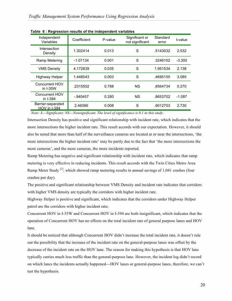
quality factors--may contribute to its occurrence. Table 6 summarizes the regression results of each of the
independent variables. Note: detailed regression results of case study II are in Appendix 14.
Table 5 : Summary of regression results
Number of observations 98 R-squared 0.3764
Adjusted R-squared 0.3279 F value 7.76
Prob > F 0.0000
Traffic Management System Performance Using Regression Analysis
20
Table 6 : Regression results of the independent variables Independent
Variables Coefficient P-value Significant or not significant
Standard error t-value
Intersection Density 1.302414 0.013 S .5143032 2.532
Ramp Metering -1.07134 0.001 S .3246102 -3.300
VMS Density 4.172839 0.035 S 1.951534 2.138
Highway Helper 1.448543 0.003 S .4695155 3.085
Concurrent HOV in I-35W .2315502 0.788 NS .8564734 0.270
Concurrent HOV in I-394 -.940457 0.280 NS .8653702 -1.087
Barrier-separated HOV in I-394
2.46086 0.008 S .9012703 2.730
Note: S---Significant; NS---Nonsignificant. The level of significance is 0.1 in this study.
Intersection Density has positive and significant relationship with incident rate, which indicates that the
more intersections the higher incident rate. This result accords with our expectation. However, it should
also be noted that more than half of the surveillance cameras are located at or near the intersections, ‘the
more intersections the higher incident rate’ may be partly due to the fact that ‘the more intersections the
more cameras’, and the more cameras, the more incidents reported.
Ramp Metering has negative and significant relationship with incident rate, which indicates that ramp
metering is very effective in reducing incidents. This result accords with the Twin Cities Metro Area
Ramp Meter Study [2], which showed ramp metering results in annual savings of 1,041 crashes (four
crashes per day).
The positive and significant relationship between VMS Density and incident rate indicates that corridors
with higher VMS density are typically the corridors with higher incident rate.
Highway Helper is positive and significant, which indicates that the corridors under Highway Helper
patrol are the corridors with higher incident rate;
Concurrent HOV in I-35W and Concurrent HOV in I-394 are both insignificant, which indicates that the
operation of Concurrent HOV has no effects on the total incident rate of general purpose lanes and HOV
lane.
It should be noticed that although Concurrent HOV didn’t increase the total incident rate, it doesn’t rule
out the possibility that the increase of the incident rate on the general-purpose lanes was offset by the
decrease of the incident rate on the HOV lane. The reason for making this hypothesis is that HOV lane
typically carries much less traffic than the general-purpose lane. However, the incident log didn’t record
on which lanes the incidents actually happened---HOV lanes or general-purpose lanes, therefore, we can’t
test the hypothesis.

Traffic Management System Performance Using Regression Analysis
21
Barrier-separated HOV in I-394 is positive and significant (as high as 2.4), which indicates that the
operation of Barrier-separated HOV is strongly associated with the increase in the total incident rate of
general purpose lanes and HOV lanes. This result accords with public dissatisfaction about HOV ----
causing incident increase.
6. Conclusion: This study used the multiple regression model to evaluate the long-run performance of four traffic
management systems --- Ramp Metering System, Variable Message Signs (VMS), Highway Helper
Program, and High Occupancy Vehicle (HOV) System in the Twin Cities metro area. Link speed and
incident rate were employed as the response variable separately for case study I and case study II.
In case study I, a huge database of about 40,000 observations covering three years’ data was established.
The long-run and systemwide performances of the four traffic management systems were estimated for
both incident-free and incident cases. The key findings are summarized as follows:
For incident-free case, ramp metering is effective in increasing mainline speed. For example,
from 7:00AM to 8:00AM, the corridor segment with ramp metering is estimated to be 4.8 mile/hr
faster than the corridor segment without ramp metering; and the effect of one ramp meter on
mainline speed is approximately equal to decreasing 60 vehicles per mile on a three-lane freeway
segment. For incident case however, corridor segments with ramp metering are not necessarily
faster or slower than corridor segments without ramp metering, which indicates the effects of the
ramp metering in increasing mainline speed won’t always offset the incident influences.
For both incident-free and incident case, the corridor segment within VMS impacting range will
be lower than the corridor segment outside. The negative relationship should be due to two
reasons: 1. VMS messages’ impacts on drivers’ behaviors; 2. the geographic distribution
characteristics of the VMSs .
Highway Helper Program was evaluated only in the incident case. The Highway Helper Program
dummy coefficient for 7:00AM-8:00AM and 8:00AM-9:00AM are positive and significant,
which indicates that in this case, the corridor segments within highway helper patrol areas will be
faster than the corridor segments out of the areas. However, the Highway Helper Program dummy
coefficient for 4:00PM-5:00PM and 5:00PM-6:00PM are insignificant, which may be due to the
sample size problem or may be due to the fact that the incident impact on speed is not in one
direction ---although the speed on corridors covered by highway helper program can be increased
(if any), the speed on corridors out of highway helper program won’t necessarily decrease.
In incident-free case, the operation of HOV lanes is associated with lower speed on the general-
purpose lanes.
Traffic Management System Performance Using Regression Analysis
22
In case study II, incident rate analysis was based on the incident data collected for two periods in Fall
2000 --- before ramp metering system shut-down and during ramp metering system shut-down. The key
findings are summarized as below:
Ramp Metering system is associated with a lower incident rate; because we tested the same
sections with and without meters, we believe this is a causal effect;
Both the corridors with higher VMS density and the corridors under Highway Helper patrol are
typically the corridors with higher incident rate;
The operation of Concurrent HOV doesn’t have a significant relationship with incident rate
change; however, we can not rule out the possibility that the increase of the incident rate on the
general-purpose lanes was offset by the decrease of the incident rate on the HOV lane (or vice
versa);
The operation of Barrier-separated HOV is associated with the increase of the total incident rate
of general purpose lanes and HOV lanes;
In future work, improvement could be made through the following aspects:
For ramp metering evaluation, the current speed regression model provided a ‘conservative’
estimate, which should be less than the full effects of ramp metering on mainline speed. An
improved model should be able to estimate the part of ramp metering’s effects on controlling
mainline density which was not explained by the ramp metering dummy.
Our study found the negative relationship between VMS impacting range and mainline speed. But
we didn’t’ answer the question whether the speed decrease at one corridor (VMS impacting range)
really help prevent more serious congestion at some other corridors. More detailed study should
be done to give a comprehensive evaluation of VMS.
For HOV system, we got the conclusion that the operation of HOV lanes is associated with lower
speed on the general-purpose lanes. However, since the purpose of HOV system is to reduce
system PHT (person hours traveled), further study must be done to determine whether the person-
hours increase on general-purpose lanes (if any) could be offset by the person-hours decrease on
HOV lanes (or vice versa).
Decreasing data-limitations. A major issue in regression analysis is the quality of database.
Regression analysis provides information on relationships between a response variable and
predictor variables but only to the degree that such information is contained in the database [6].
Due to data quality, the analysis of HOV system can’t be conducted in incident case. Also, the
evaluation of VMS is limited by the lack of detailed activity log. In addition, restricted by the
earlier years’ incident data quality, we just used the incident data in Fall 2000 for incident rate

Traffic Management System Performance Using Regression Analysis
23
regression analysis. The limited study periods lead to the selection of long corridors, which
prevented us from employing detailed link traffic and infrastructure characteristics as predictor
variables.

Traffic Management System Performance Using Regression Analysis
24
References:
1. Banks, James H. Kelly, Gregory (1997). Traffic Management Systems Performance
Measurement Final Report. California PATH Research Report (UCB-ITS-PRR-97-53).
2. Cambridge Systematics, Inc (2001). Twin Cities Metro Area Ramp Meter Study. Final report
prepared for Minnesota Department of Transportation.
http://www.dot.state.mn.us/rampmeterstudy/reports.html.
3. Cambridge Systematics, Inc (2002). Twin Cities HOV Study. Final report prepared for
Minnesota Department of Transportation. http://www.dot.state.mn.us/information/hov/.
4. Cook, R. Dennis. Applied regression including computing and graphics. Published by John
Wiley & Sons, Inc. 1999.
5. DeGroot, Morris H. Probability and statistics, 2nd ed. Published by Addison-Wesley Pub.
Co., c1986.
6. Gunst, Richard F. Mason, Robert L. Regression analysis and its application: a data-oriented
approach. Published by M. Dekker, c1980, New York.
7. Hall, Fred L. Traffic Flow Theory: A State of the Art Report, Chapter 2: Traffic Stream
Characteristics. Sponsored by the Transportation Research Board's Committee on Theory of
Traffic Flow (A3A11), funded by Federal Highway Administration (FHWA) in June 1992.
http://www-cta.ornl.gov/cta/research/trb/tft.html
8. Institute of Transportation Engineers (ITE). Manual of Traffic Engineering Studies, 3rd ed.
Washington, 1964.
9. Levinson, David Zhang, Lei Das, Shantanu Sheikh, Atif (2002) Ramp Meters on Trial:
Evidence from the Twin Cities Ramp Meters Shut-off. Presented at 81st Transportation Research
Board Conference, Washington DC 2002 (TRB-02-2167).
10. Levinson, David (2002). Perspectives on Efficiency in Transportation. Presented at the 81st
Transportation Research Board Conference, Washington DC 2002 (TRB-02-2015).

Traffic Management System Performance Using Regression Analysis
25
11. Minnesota Department of Transportation (2000 and 2001). Freeway Traffic Management
Program Status Report. http://depts.washington.edu/trba3a09/status/jan2001/Minnesota.pdf .
http://depts.washington.edu/trba3a09/status/jun2000/minnesota.pdf.
12. Minnesota Department of Transportation Traffic Management Center.
http://www.dot.state.mn.us/tmc/.

Traffic Management System Performance Using Regression Analysis
26
Appendix 1. Case study I: Corridor selection

Traffic Management System Performance Using Regression Analysis
27
Appendix 2. Case study I: Corridor selection
Corridor Geographic characteristics From To
I-494NB Beltline freeway CR 6 I-94
I-494SB Beltline freeway Bass Lake Rd CR 6
I-494WB Beltline freeway I-35W TH 169
I-494EB Beltline freeway TH 169 I-35W
I-694WB Beltline freeway I-35W TH 252
I-694EB Beltline freeway TH 252 I-35W
I-94WB Intercity connector I-35E TH 280
I-94EB Intercity connector TH 280 I-35E
I-94NB Radial freeway within the I-494/I-694 beltline Broadway Humboldt
I-94SB Radial freeway within the I-494/I-694 beltline Humboldt TH 55
I-394WB Radial freeway within the I-494/I-694 beltline I-94 TH 100
I-394EB Radial freeway within the I-494/I-694 beltline TH 100 I-94
I-35E NB (North of I-94) Radial freeway within the I-494/I-694 beltline I-94 TH 36
I-35E SB (North of I-94) Radial freeway within the I-494/I-694 beltline TH 36 I-94
I-35E NB (South of I-94) Radial freeway within the I-494/I-694 beltline I-494 ST. Clair
I-35E SB (South of I-94) Radial freeway within the I-494/I-694 beltline 5TH Kellogg I-494
I-35W NB Radial freeway outside the I-494/I-694 beltline Mississippi River 86TH
I-35W SB Radial freeway outside the I-494/I-694 beltline 86TH 113TH ST.
I-35E NB (South of I-494) Radial freeway outside the I-494/I-694 beltline CR 11 Diffley RD.
I-35E SB (South of I-494) Radial freeway outside the I-494/I-694 beltline Diffley RD. TH-77
TH-77 NB Radial freeway outside the I-494/I-694 beltline 127TH Old Shakopee
TH-77 SB Radial freeway outside the I-494/I-694 beltline Old Shakopee I-35E

Traffic Management System Performance Using Regression Analysis
28
Appendix 3. Case study I: The correlation matrixes of predictor variables
I. Incident-free:
7:00AM-8:00AM DENSITY RM VMS ConHOV BarHOV
8:00AM-9:00AM DENSITY RM VMS ConHOV BarHOV
DENSITY 1.00 0.19 -0.13 0.08 0.06 DENSITY 1.00 0.19 -0.09 0.15 0.07 RM 0.19 1.00 0.01 -0.03 -0.03 RM 0.19 1.00 0.02 -0.03 -0.03
VMS -0.13 0.01 1.00 -0.05 -0.05 VMS -0.09 0.02 1.00 -0.04 -0.05 ConHOV 0.08 -0.03 -0.05 1.00 -0.05 ConHOV 0.15 -0.03 -0.04 1.00 -0.05 BarHOV 0.06 -0.03 -0.05 -0.05 1.00 BarHOV 0.07 -0.03 -0.05 -0.05 1.00
4:00PM-5:00PM DENSITY RM VMS ConHOV BarHOV
5:00PM-6:00PM DENSITY RM VMS ConHOV BarHOV
DENSITY 1.00 0.09 0.07 0.15 0.08 DENSITY 1.00 0.07 0.07 0.12 0.13 RM 0.09 1.00 0.01 -0.03 -0.03 RM 0.07 1.00 0.01 -0.02 -0.03
VMS 0.07 0.01 1.00 -0.05 -0.04 VMS 0.07 0.01 1.00 -0.05 -0.04 ConHOV 0.15 -0.03 -0.05 1.00 -0.05 ConHOV 0.12 -0.02 -0.05 1.00 -0.05 BarHOV 0.08 -0.03 -0.04 -0.05 1.00 BarHOV 0.13 -0.03 -0.04 -0.05 1.00
II. Incident:
7:00AM-8:00AM DENSITY RM VMS HHELPER ConHOV BarHOV
8:00AM-9:00AM DENSITY RM VMS HHELPER ConHOV BarHOV
DENSITY 1.00 -0.11 -0.32 -0.03 0.05 0.02 DENSITY 1.00 0.10 -0.14 0.22 0.01 -0.02 RM -0.11 1.00 0.16 0.29 -0.12 -0.08 RM 0.10 1.00 0.05 0.28 -0.07 -0.07
VMS -0.32 0.16 1.00 0.25 -0.10 -0.04 VMS -0.14 0.05 1.00 0.17 -0.14 -0.03 HHELPER -0.03 0.29 0.25 1.00 0.08 0.10 HHELPER 0.22 0.28 0.17 1.00 0.04 0.13 ConHOV 0.05 -0.12 -0.10 0.08 1.00 -0.05 ConHOV 0.01 -0.07 -0.14 0.04 1.00 -0.04 BarHOV 0.02 -0.08 -0.04 0.10 -0.05 1.00 BarHOV -0.02 -0.07 -0.03 0.13 -0.04 1.00
4:00PM-5:00PM DENSITY RM VMS HHELPER ConHOV BarHOV
5:00PM-6:00PM DENSITY RM VMS HHELPER ConHOV BarHOV
DENSITY 1.00 0.02 0.10 0.12 0.03 0.02 DENSITY 1.00 -0.12 0.15 0.09 0.15 -0.02 RM 0.02 1.00 -0.03 0.32 -0.27 -0.11 RM -0.12 1.00 -0.03 0.36 -0.37 -0.05
VMS 0.10 -0.03 1.00 -0.07 -0.02 -0.17 VMS 0.15 -0.03 1.00 0.10 0.07 -0.13 HHELPER 0.12 0.32 -0.07 1.00 0.05 0.09 HHELPER 0.09 0.36 0.10 1.00 0.06 0.13 ConHOV 0.03 -0.27 -0.02 0.05 1.00 -0.07 ConHOV 0.15 -0.37 0.07 0.06 1.00 -0.05 BarHOV 0.02 -0.11 -0.17 0.09 -0.07 1.00 BarHOV -0.02 -0.05 -0.13 0.13 -0.05 1.00

Traffic Management System Performance Using Regression Analysis
29
Appendix 4. Case study II: Corridor selection
Traffic Management System Performance Using Regression Analysis
30
Appendix 5. Case study II: Facility status for the 26 corridors
Corridor Direction Ramp Meter (1, 0)
# of Variable Message
Signs
Highway Helper
Program (1, 0)
Concurrent HOV in I-35W
(1, 0)
Concurrent HOV in I-394
(1, 0)
Barrier-separated HOV in I-394(1, 0)
1N 1 1 1 0 0 0 1 1S 1 1 1 0 0 0 2N 1 1 1 0 0 0 2 2S 1 1 1 0 0 0 3W 1 1 1 0 0 1 3 3E 1 1 1 0 0 1 4W 1 1 1 0 1 0 4 4E 1 3 1 0 1 0 5N 1 1 1 1 0 0 5 5S 1 0 1 1 0 0 6N 1 1 1 0 0 0 6 6S 1 1 1 0 0 0 7N 1 1 1 0 0 0 7 7S 1 2 1 0 0 0 8N 1 2 1 0 0 0 8 8S 1 1 1 0 0 0 9N 1 0 0 0 0 0 9 9S 1 1 0 0 0 0 10W 1 1 1 0 0 0 10 10E 1 2 1 0 0 0 11W 1 1 0 0 0 0 11 11E 0 0 0 0 0 0 12W 1 1 1 0 0 0 12 12E 1 0 1 0 0 0 13N 1 1 1 0 0 0 13 13S 1 1 1 0 0 0 14W 1 3 1 0 0 0 14 14E 1 2 1 0 0 0 15N 1 1 1 0 0 0 15 15S 1 1 1 0 0 0 16N 1 1 1 0 0 0 16 16S 1 1 1 0 0 0 17W 1 1 1 0 0 0 17 17E 1 1 1 0 0 0 18N 1 1 1 0 0 0 18 18S 1 1 1 0 0 0 19N 1 1 0 0 0 0 19 19S 1 1 0 0 0 0 20N 1 1 1 0 0 0 20 20S 1 2 1 0 0 0 21W 1 1 1 0 0 0 21 21E 1 1 1 0 0 0 22N 1 0 1 0 0 0 22 22S 1 1 1 0 0 0 23N 1 1 1 0 0 0 23 23S 0 0 1 0 0 0 24N 1 1 0 0 0 0 24 24S 0 1 0 0 0 0 25W 1 2 1 0 0 0 25 25E 1 2 1 0 0 0
26 26S 1 1 0 0 0 0
Note: Ramp Meter=1 if the corridor is under ramp metering control; otherwise, Ramp Meter=0;

Traffic Management System Performance Using Regression Analysis
31
Highway Helper Program=1 if the corridor is within highway helper program patrol area; otherwise, Highway Helper Program=0; HOV=1 if the corridor has HOV lane(s) in operation; otherwise, HOV=0; For VMS, the number of VMSs per corridor per direction is counted.

Traffic Management System Performance Using Regression Analysis
32
Appendices 6-13: Case study I regression results: Appendix 6:
Regression Result: Incident Free 7:00 AM – 8:00 AM
Source SS df MS
Model 679868.109 27 25180.3003
Residual 785752.454 8960 87.6955864
Total 1465620.56 8987 163.082292
Number of obs = 8988 F( 27, 8960) = 287.13 Prob > F = 0.0000 R-squared = 0.4639 Adj R-squared = 0.4623 Root MSE = 9.3646
Response Variable : Speed
Predictor Variable Coef. Std. Err. t P>|t| [95% Conf. Interval]
Density -.2520507 .0052265 -48.226 0.000 -.2622958 -.2418056
Ramp Meter 4.828919 .2686687 17.974 0.000 4.302266 5.355571
VMS -2.703652 .266009 -10.164 0.000 -3.22509 -2.182213
Concurrent HOV -29.90661 1.013276 -29.515 0.000 -31.89286 -27.92036
Barrier-separated HOV -36.27597 .9902992 -36.631 0.000 -38.21718 -34.33475
Two-Lane 7.535965 1.073159 7.022 0.000 5.432328 9.639602
Three-Lane 6.130187 1.012318 6.056 0.000 4.145812 8.114562
Four-Lane -2.731895 .6449748 -4.236 0.000 -3.996193 -1.467596
I-35E NB (South of I-94) -28.1754 .837144 -33.657 0.000 -29.8164 -26.5344
I-35E SB (South of I-94) -28.99105 .8952893 -32.382 0.000 -30.74602 -27.23607
I-394WB 9.828056 .935602 10.505 0.000 7.994062 11.66
I-394EB dropped
I-35W NB 2.605788 .9482397 2.748 0.006 .7470215 4.464555
I-35W SB dropped
I-94WB -18.63839 1.127802 -16.526 0.000 -20.84914 -16.42764
I-94EB -14.47175 1.166032 -12.411 0.000 -16.75744 -12.18606
I-94NB -12.9372 1.18577 -10.910 0.000 -15.26158 -10.61282
I-94SB -18.07189 1.177862 -15.343 0.000 -20.38077 -15.76302
I-494NB -32.74104 .8589865 -38.116 0.000 -34.42485 -31.05723
I-494SB -37.8641 .8656379 -43.741 0.000 -39.56095 -36.16726
I-694WB -31.94825 .9041072 -35.337 0.000 -33.72051 -30.17599
I-694EB -29.9193 .9404882 -31.813 0.000 -31.76287 -28.07573
I-494WB -37.04412 .8026948 -46.150 0.000 -38.61759 -35.47066
I-494EB -32.70793 .7902354 -41.390 0.000 -34.25697 -31.15888
I-35E NB (North of I-94) dropped
I-35E SB (North of I-94) -24.03749 .8791755 -27.341 0.000 -25.76087 -22.3141
TH-77 NB -27.85155 .8477757 -32.852 0.000 -29.51338 -26.18971
TH-77 SB -24.50227 .8223942 -29.794 0.000 -26.11435 -22.89019
I-35E NB (South of I-494) -21.71335 .8592039 -25.271 0.000 -23.39758 -20.02911
I-35E SB (South of I-494) -23.27922 .9095992 -25.593 0.000 -25.06224 -21.49619
Constant 85.7969 1.363444 62.927 0.000 83.12424 88.46956

Traffic Management System Performance Using Regression Analysis
33
Appendix 7:
Regression Result: Incident Free 8:00 AM – 9:00 AM
Source SS df MS
Model 670057.196 27 24816.9332
Residual 757332.421 9002 84.1293514
Total 1427389.62 9029 158.089447
Number of obs = 9030 F( 27, 9002) = 294.99 Prob > F = 0.0000 R-squared = 0.4694 Adj R-squared = 0.4678 Root MSE = 9.1722
Response Variable : Speed
Predictor Variable Coef. Std. Err. t P>|t| [95% Conf. Interval]
Density -.250744 .0048934 -51.241 0.000 -.2603362 -.2411518
Ramp Meter 2.32501 .3405388 6.827 0.000 1.657476 2.992543
VMS -2.976521 .2591904 -11.484 0.000 -3.484594 -2.468449
Concurrent HOV -14.84777 1.189239 -12.485 0.000 -17.17895 -12.5166
Barrier-separated HOV -17.19873 .9781615 -17.583 0.000 -19.11614 -15.28131
Two-Lane 3.985557 1.050768 3.793 0.000 1.925813 6.045301
Three-Lane 2.447195 .9903281 2.471 0.013 .5059265 4.388463
Four-Lane -2.807352 .6272801 -4.475 0.000 -4.036964 -1.577741
I-35E NB (South of I-94) -8.54995 1.022211 -8.364 0.000 -10.55372 -6.546185
I-35E SB (South of I-94) -11.62804 1.075206 -10.815 0.000 -13.73569 -9.520388
I-394WB 8.339799 .9353119 8.917 0.000 6.506375 10.17322
I-394EB dropped
I-35W NB 2.864719 .9247433 3.098 0.002 1.052012 4.677427
I-35W SB dropped
I-94WB -5.100248 .7153619 -7.130 0.000 -6.50252 -3.697976
I-94EB -.7432851 .7306705 -1.017 0.309 -2.175566 .6889953
I-94NB dropped
I-94SB -3.079926 .63322 -4.864 0.000 -4.321181 -1.838671
I-494NB -16.7402 1.071966 -15.616 0.000 -18.8415 -14.6389
I-494SB -21.30695 1.042088 -20.446 0.000 -23.34968 -19.26422
I-694WB -16.12696 .9598869 -16.801 0.000 -18.00856 -14.24537
I-694EB -15.96904 .9537183 -16.744 0.000 -17.83855 -14.09954
I-494WB -19.48569 1.003758 -19.413 0.000 -21.45328 -17.5181
I-494EB -14.49763 1.02189 -14.187 0.000 -16.50076 -12.49449
I-35E NB (North of I-94) 17.21254 1.160998 14.826 0.000 14.93672 19.48836
I-35E SB (North of I-94) .4036325 1.087084 0.371 0.710 -1.727299 2.534564
TH-77 NB -6.986283 1.04779 -6.668 0.000 -9.040189 -4.932376
TH-77 SB -9.453598 1.034841 -9.135 0.000 -11.48212 -7.425074
I-35E NB (South of I-494) -6.233243 1.07325 -5.808 0.000 -8.337058 -4.129428
I-35E SB (South of I-494) -9.912644 1.13259 -8.752 0.000 -12.13278 -7.69251
Constant 72.88782 .7421147 98.216 0.000 71.43311 74.34254

Traffic Management System Performance Using Regression Analysis
34
Appendix 8:
Regression Result: Incident Free 4:00 PM – 5:00 PM
Source SS df MS
Model 1025131.45 27 37967.8313
Residual 740601.928 8909 83.1296361
Total 1765733.37 8936 197.597737
Number of obs = 8937 F( 27, 8909) = 456.73 Prob > F = 0.0000 R-squared = 0.5806 Adj R-squared = 0.5793 Root MSE = 9.1175
Response Variable : Speed
Predictor Variable Coef. Std. Err. t P>|t| [95% Conf. Interval]
Density -.2617367 .0048644 -53.806 0.000 -.2712721 -.2522014 Ramp Meter 3.931768 .2635107 14.921 0.000 3.415226 4.44831 VMS -3.115385 .2563565 -12.153 0.000 -3.617903 -2.612867 Concurrent HOV -22.04745 1.198693 -18.393 0.000 -24.39717 -19.69774 Barrier-separated HOV -27.93467 .9876593 -28.284 0.000 -29.8707 -25.99863 Two-Lane 3.267593 1.050682 3.110 0.002 1.208015 5.327171 Three-Lane 1.42601 .984605 1.448 0.148 -.5040425 3.356062 Four-Lane -4.313578 .625837 -6.892 0.000 -5.540363 -3.086793
I-35E NB (South of I-94) -15.93184 1.023887 -15.560 0.000 -17.9389 -13.92479
I-35E SB (South of I-94) -20.43802 1.077617 -18.966 0.000 -22.5504 -18.32564
I-394WB 7.170408 .9321031 7.693 0.000 5.343271 8.997544
I-394EB dropped
I-35W NB 5.530335 .9157479 6.039 0.000 3.735258 7.325412
I-35W SB dropped
I-94WB -6.202389 .7246358 -8.559 0.000 -7.622842 -4.781936
I-94EB -12.82244 .745279 -17.205 0.000 -14.28335 -11.36152
I-94NB dropped I-94SB -12.21012 .6634801 -18.403 0.000 -13.51069 -10.90954
I-494NB -23.20866 1.104958 -21.004 0.000 -25.37463 -21.04269
I-494SB -27.36845 1.055263 -25.935 0.000 -29.43701 -25.29989
I-694WB -18.40719 .9556491 -19.261 0.000 -20.28049 -16.5339
I-694EB -22.41605 .9589654 -23.375 0.000 -24.29584 -20.53626
I-494WB -28.239 1.001128 -28.207 0.000 -30.20144 -26.27656
I-494EB -31.8136 1.023151 -31.094 0.000 -33.81921 -29.80799
I-35E NB (North of I-94) 1.193324 1.157474 1.031 0.303 -1.075592 3.46224
I-35E SB (North of I-94) -1.511027 1.090152 -1.386 0.166 -3.647977 .6259223
TH-77 NB -12.31031 1.058612 -11.629 0.000 -14.38543 -10.23518
TH-77 SB -6.749128 1.01518 -6.648 0.000 -8.739115 -4.759141
I-35E NB (South of I-494) -14.73363 1.085274 -13.576 0.000 -16.86102 -12.60625
I-35E SB (South of I-494) -8.384499 1.104516 -7.591 0.000 -10.5496 -6.219394
Constant 81.2317 .7315499 111.041 0.000 79.79769 82.66571

Traffic Management System Performance Using Regression Analysis
35
Appendix 9:
Regression Result: Incident Free 5:00 PM – 6:00 PM
Source SS df MS
Model 1232647.11 27 45653.5968
Residual 812976.66 8860 91.758088
Total 2045623.77 8887 230.181588
Number of obs = 8888 F( 27, 8860) = 497.54 Prob > F = 0.0000 R-squared = 0.6026 Adj R-squared = 0.6014 Root MSE = 9.579
Response Variable : Speed
Predictor Variable Coef. Std. Err. t P>|t| [95% Conf. Interval]
Density -.3012855 .0050181 -60.040 0.000 -.3111221 -.2914489 Ramp Meter 4.802929 .277239 17.324 0.000 4.259476 5.346382 VMS -3.321087 .2704075 -12.282 0.000 -3.851148 -2.791025 Concurrent HOV -9.621244 1.241572 -7.749 0.000 -12.05501 -7.187475 Barrier-separated HOV -17.54004 .9975423 -17.583 0.000 -19.49545 -15.58462 Two-Lane 1.175207 1.107088 1.062 0.288 -.9949418 3.345355 Three-Lane -.6882897 1.036549 -0.664 0.507 -2.720166 1.343586 Four-Lane -5.102936 .6597504 -7.735 0.000 -6.3962 -3.809673
I-35E NB (South of I-94) -3.42142 1.023239 -3.344 0.001
-5.427206 -1.415634
I-35E SB (South of I-94) -9.533662 1.091208 -8.737 0.000 -11.67268 -7.394641
I-394WB 3.123899 .9828605 3.178 0.001 1.197265 5.050534
I-394EB dropped
I-35W NB 8.649375 .9564371 9.043 0.000 6.774537 10.52421
I-35W SB dropped
I-94WB 4.070565 .6725108 6.053 0.000 2.752288 5.388842
I-94EB -2.511493 .6818111 -3.684 0.000 -3.848001 -1.174986
I-94NB 11.30397 .6962579 16.235 0.000 9.93914 12.66879 I-94SB dropped
I-494NB -9.051848 1.145056 -7.905 0.000 -11.29642 -6.807273
I-494SB -14.25209 1.04764 -13.604 0.000 -16.30571 -12.19847
I-694WB -5.903079 .9476044 -6.229 0.000 -7.760603 -4.045555
I-694EB -10.85954 .9358015 -11.605 0.000 -12.69393 -9.025151
I-494WB -14.13135 1.017796 -13.884 0.000 -16.12647 -12.13624
I-494EB -19.42545 1.068696 -18.177 0.000 -21.52034 -17.33056
I-35E NB (North of I-94) 13.97171 1.219328 11.459 0.000 11.58155 16.36188
I-35E SB (North of I-94) 11.52134 1.112561 10.356 0.000 9.340462 13.70222
TH-77 NB .4110926 1.050325 0.391 0.696 -1.647788 2.469973
TH-77 SB 5.749565 1.025583 5.606 0.000 3.739185 7.759945
I-35E NB (South of I-494) -1.510314 1.091921 -1.383 0.167 -3.650733 .6301047
I-35E SB (South of I-494) 5.516165 1.127045 4.894 0.000 3.306896 7.725434
Constant 71.344 .644671 110.667 0.000 70.08029 72.6077
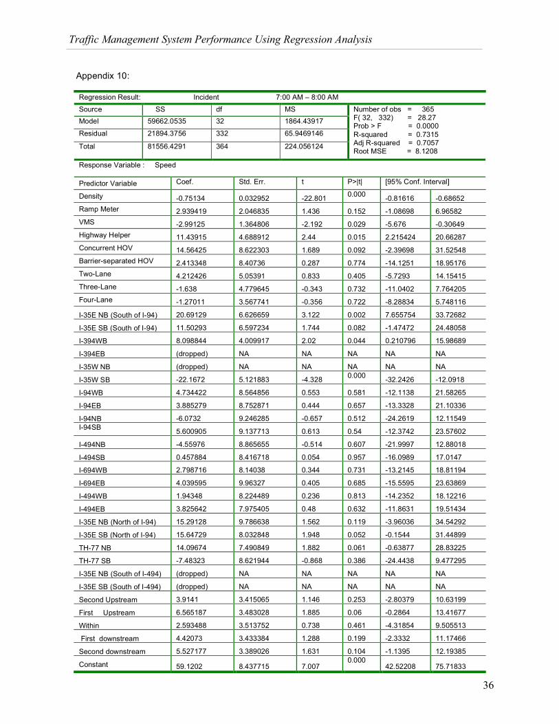
Traffic Management System Performance Using Regression Analysis
36
Appendix 10:
Regression Result: Incident 7:00 AM – 8:00 AM
Source SS df MS Model 59662.0535 32 1864.43917
Residual 21894.3756 332 65.9469146
Total 81556.4291 364 224.056124
Number of obs = 365 F( 32, 332) = 28.27 Prob > F = 0.0000 R-squared = 0.7315 Adj R-squared = 0.7057 Root MSE = 8.1208
Response Variable : Speed
Predictor Variable Coef. Std. Err. t P>|t| [95% Conf. Interval]
Density -0.75134 0.032952 -22.801 0.000 -0.81616 -0.68652 Ramp Meter 2.939419 2.046835 1.436 0.152 -1.08698 6.96582 VMS -2.99125 1.364806 -2.192 0.029 -5.676 -0.30649 Highway Helper 11.43915 4.688912 2.44 0.015 2.215424 20.66287 Concurrent HOV 14.56425 8.622303 1.689 0.092 -2.39698 31.52548 Barrier-separated HOV 2.413348 8.40736 0.287 0.774 -14.1251 18.95176 Two-Lane 4.212426 5.05391 0.833 0.405 -5.7293 14.15415 Three-Lane -1.638 4.779645 -0.343 0.732 -11.0402 7.764205 Four-Lane -1.27011 3.567741 -0.356 0.722 -8.28834 5.748116
I-35E NB (South of I-94) 20.69129 6.626659 3.122 0.002 7.655754 33.72682
I-35E SB (South of I-94) 11.50293 6.597234 1.744 0.082 -1.47472 24.48058
I-394WB 8.098844 4.009917 2.02 0.044 0.210796 15.98689
I-394EB (dropped) NA NA NA NA NA
I-35W NB (dropped) NA NA NA NA NA
I-35W SB -22.1672 5.121883 -4.328 0.000 -32.2426 -12.0918
I-94WB 4.734422 8.564856 0.553 0.581 -12.1138 21.58265
I-94EB 3.885279 8.752871 0.444 0.657 -13.3328 21.10336
I-94NB -6.0732 9.246285 -0.657 0.512 -24.2619 12.11549 I-94SB 5.600905 9.137713 0.613 0.54 -12.3742 23.57602
I-494NB -4.55976 8.865655 -0.514 0.607 -21.9997 12.88018
I-494SB 0.457884 8.416718 0.054 0.957 -16.0989 17.0147
I-694WB 2.798716 8.14038 0.344 0.731 -13.2145 18.81194
I-694EB 4.039595 9.96327 0.405 0.685 -15.5595 23.63869
I-494WB 1.94348 8.224489 0.236 0.813 -14.2352 18.12216
I-494EB 3.825642 7.975405 0.48 0.632 -11.8631 19.51434
I-35E NB (North of I-94) 15.29128 9.786638 1.562 0.119 -3.96036 34.54292
I-35E SB (North of I-94) 15.64729 8.032848 1.948 0.052 -0.1544 31.44899
TH-77 NB 14.09674 7.490849 1.882 0.061 -0.63877 28.83225
TH-77 SB -7.48323 8.621944 -0.868 0.386 -24.4438 9.477295
I-35E NB (South of I-494) (dropped) NA NA NA NA NA
I-35E SB (South of I-494) (dropped) NA NA NA NA NA
Second Upstream
3.9141 3.415065 1.146 0.253 -2.80379 10.63199
First Upstream 6.565187 3.483028 1.885 0.06 -0.2864 13.41677
Within 2.593488 3.513752 0.738 0.461 -4.31854 9.505513
First downstream 4.42073 3.433384 1.288 0.199 -2.3332 11.17466
Second downstream 5.527177 3.389026 1.631 0.104 -1.1395 12.19385
Constant 59.1202 8.437715 7.007 0.000
42.52208 75.71833

Traffic Management System Performance Using Regression Analysis
37
Appendix 11:
Regression Result: Incident 8:00 AM – 9:00 AM
Source SS df MS
Model 66054.0979 31 2130.77735
Residual 21355.1839 338 63.1810173
Total 87409.2818 369 236.881522
Number of obs = 370 F( 31, 338) = 33.72 Prob > F = 0.0000 R-squared = 0.7557 Adj R-squared = 0.7333 Root MSE = 7.9486
Response Variable : Speed Predictor Variable Coef. Std. Err. t P>|t| [95% Conf. Interval]
Density -0.58161 0.025821 -22.525 0.000 -0.6324 -0.53082
Ramp Meter -0.30668 2.295615 -0.134 0.894 -4.82218 4.208806
VMS -3.24461 1.267541 -2.56 0.011 -5.73788 -0.75135
Highway Helper 9.254188 5.386158 1.718 0.087 -1.34042 19.8488
Concurrent HOV -9.42419 8.124675 -1.16 0.247 -25.4055 6.557106
Barrier-separated HOV -4.58715 7.47346 -0.614 0.54 -19.2875 10.1132
Two-Lane 9.255993 5.985023 1.547 0.123 -2.51659 21.02858
Three-Lane 5.030859 5.725138 0.879 0.38 -6.23053 16.29225
Four-Lane 3.760379 4.824998 0.779 0.436 -5.73043 13.25118
I-35E NB (South of I-94) 13.46424 5.05378 2.664 0.008 3.523422 23.40507
I-35E SB (South of I-94) 8.833973 5.14211 1.718 0.087 -1.28059 18.94854
I-394WB 9.948754 2.862385 3.476 0.001 4.318422 15.57909
I-394EB (dropped) NA NA NA NA NA
I-35W NB (dropped) NA NA NA NA NA
I-35W SB (dropped) NA NA NA NA NA
I-94WB -2.68063 7.83222 -0.342 0.732 -18.0867 12.7254
I-94EB 0.278481 8.087543 0.034 0.973 -15.6298 16.18674
I-94NB (dropped) NA NA NA NA NA
I-94SB 9.17277 8.681812 1.057 0.291 -7.90442 26.24996
I-494NB -8.78545 7.66078 -1.147 0.252 -23.8543 6.283365
I-494SB -10.9113 7.472835 -1.46 0.145 -25.6104 3.787851
I-694WB -6.12374 7.432362 -0.824 0.411 -20.7433 8.495773
I-694EB -8.97463 7.984406 -1.124 0.262 -24.68 6.730754
I-494WB -8.32298 7.310257 -1.139 0.256 -22.7023 6.056346
I-494EB -3.9852 7.119562 -0.56 0.576 -17.9894 10.01903
I-35E NB (North of I-94) 32.43377 8.535746 3.8 0.000 15.6439 49.22364
I-35E SB (North of I-94) 5.057576 7.278934 0.695 0.488 -9.26014 19.37529
TH-77 NB 5.548112 6.789061 0.817 0.414 -7.80602 18.90224
TH-77 SB -8.73279 8.196889 -1.065 0.287 -24.8561 7.39055
I-35E NB (South of I-494) 2.848957 7.739737 0.368 0.713 -12.3752 18.07308
I-35E SB (South of I-494) (dropped) NA NA NA NA NA
Second Upstream
-2.13123 1.796087 -1.187 0.236 -5.66415 1.401683
First Upstream 0.133774 1.791197 0.075 0.941 -3.38952 3.657072
Within -4.36745 2.088316 -2.091 0.037 -8.47518 -0.25972
First downstream 0.631739 1.81047 0.349 0.727 -2.92947 4.192946
Second downstream 1.665056 1.835205 0.907 0.365 -1.94481 5.274918
Constant 63.18793 7.581401 8.335 0.000 48.27526 78.1006
Appendix6:

Traffic Management System Performance Using Regression Analysis
38
Appendix 12:
Regression Result: Incident 4:00 PM – 5:00 PM
Source SS df MS Model 84309.3485 32 2634.66714
Residual 27232.0062 354 76.9265712
Total 111541.355 386 288.96724
Number of obs = 387 F( 32, 354) = 34.25 Prob > F = 0.0000 R-squared = 0.7559
Adj R-squared = 0.7338 Root MSE = 8.7708
Response Variable : Speed
Predictor Variable Coef. Std. Err. t P>|t| [95% Conf. Interval]
Density -0.50266 0.024991 -20.114 0.000 -0.55181 -0.45352
Ramp Meter 4.101622 2.119897 1.935 0.054 -0.06755 8.270798
VMS -5.93651 1.422739 -4.173 0.000 -8.73459 -3.13842
Highway Helper 8.453485 8.276665 1.021 0.308 -7.82413 24.7311
Concurrent HOV -15.7892 6.549702 -2.411 0.016 -28.6704 -2.90799
Barrier-separated HOV -12.5542 5.96706 -2.104 0.036 -24.2896 -0.81889
Two-Lane 7.865736 6.172571 1.274 0.203 -4.27379 20.00526
Three-Lane 4.896097 5.818955 0.841 0.401 -6.54797 16.34016
Four-Lane 0.361771 4.701626 0.077 0.939 -8.88486 9.608402
I-35E NB (South of I-94) -6.28741 8.299102 -0.758 0.449 -22.6092 10.03434
I-35E SB (South of I-94) -2.06567 6.979932 -0.296 0.767 -15.793 11.66168
I-394WB (dropped) NA NA NA NA NA
I-394EB -2.84497 3.235557 -0.879 0.38 -9.2083 3.518355
I-35W NB 11.66681 4.886601 2.388 0.017 2.056392 21.27723
I-35W SB (dropped) NA NA NA NA NA
I-94WB -0.06946 4.729215 -0.015 0.988 -9.37035 9.231431
I-94EB -8.31375 4.546734 -1.829 0.068 -17.2558 0.628263
I-94NB (dropped) NA NA NA NA NA
I-94SB -5.35033 4.932028 -1.085 0.279 -15.0501 4.349429
I-494NB -14.1119 6.54738 -2.155 0.032 -26.9885 -1.23521
I-494SB -17.8651 8.305069 -2.151 0.032 -34.1986 -1.53166
I-694WB -8.79731 5.993604 -1.468 0.143 -20.5849 2.990238
I-694EB -16.3445 5.493882 -2.975 0.003 -27.1493 -5.53977
I-494WB -20.1711 5.547078 -3.636 0.000 -31.0804 -9.2617
I-494EB -17.6815 5.592347 -3.162 0.002 -28.6799 -6.68311
I-35E NB (North of I-94) 6.590165 5.998975 1.099 0.273 -5.20795 18.38827
I-35E SB (North of I-94) 1.114478 6.045083 0.184 0.854 -10.7743 13.00327
TH-77 NB -1.82628 7.101842 -0.257 0.797 -15.7934 12.14083
TH-77 SB 0.62628 6.122055 0.102 0.919 -11.4139 12.66645
I-35E NB (South of I-494) (dropped) NA NA NA NA NA
I-35E SB (South of I-494) 10.07079 9.044946 1.113 0.266 -7.71779 27.85938
Second Upstream
-3.80463 1.868951 -2.036 0.043 -7.48028 -0.12899
First Upstream -3.92623 1.805705 -2.174 0.03 -7.47749 -0.37497
Within -4.96945 1.893313 -2.625 0.009 -8.693 -1.24589
First downstream -1.74078 1.705062 -1.021 0.308 -5.09411 1.61254
Second downstream -0.20719 1.790329 -0.116 0.908 -3.72821 3.313829
Constant 71.22278 9.356426 7.612 0.000 52.82161 89.62395

Traffic Management System Performance Using Regression Analysis
39
Appendix 13:
Regression Result: Incident 5:00 PM – 6:00 PM
Source SS df MS
Model 85473.1091 33 2590.09422
Residual 38396.3819 392 97.9499538
Total 123869.491 425 291.457626
Number of obs = 426 F( 33, 392) = 26.44 Prob > F = 0.0000 R-squared = 0.6900 Adj R-squared = 0.6639 Root MSE = 9.897
Response Variable : Speed
Predictor Variable Coef. Std. Err. t P>|t| [95% Conf. Interval]
Density -0.46693 0.023679 -19.719 0.000 -0.51348 -0.42038 Ramp Meter 6.54014 2.523434 2.592 0.01 1.578982 11.5013 VMS -3.75248 1.443685 -2.599 0.01 -6.59082 -0.91415 Highway Helper -1.59986 14.23486 -0.112 0.911 -29.5861 26.38636 Concurrent HOV -1.01735 16.35707 -0.062 0.95 -33.1759 31.14121 Barrier-separated HOV -6.80054 15.05689 -0.452 0.652 -36.4029 22.80182 Two-Lane 16.08981 6.328272 2.543 0.011 3.648209 28.53141 Three-Lane 11.46823 6.047429 1.896 0.059 -0.42122 23.35768 Four-Lane 6.510261 4.646011 1.401 0.162 -2.62395 15.64448
I-35E NB (South of I-94) -6.07534 4.673565 -1.3 0.194 -15.2637 3.11305
I-35E SB (South of I-94) -9.9797 5.11016 -1.953 0.052 -20.0264 0.067051
I-394WB (dropped) NA NA NA NA NA
I-394EB -1.44766 3.5831 -0.404 0.686 -8.49216 5.596832
I-35W NB (dropped) NA NA NA NA NA
I-35W SB -9.74654 8.226623 -1.185 0.237 -25.9204 6.427283
I-94WB 0.994062 15.41102 0.065 0.949 -29.3045 31.29266
I-94EB -3.21353 15.44811 -0.208 0.835 -33.585 27.15798
I-94NB 33.62636 15.90456 2.114 0.035 2.357456 64.89527 I-94SB 5.636396 15.9536 0.353 0.724 -25.7289 37.00171
I-494NB -9.4713 15.35901 -0.617 0.538 -39.6676 20.72504
I-494SB -13.8898 15.5389 -0.894 0.372 -44.4398 16.6602
I-694WB -2.41808 15.50913 -0.156 0.876 -32.9096 28.0734
I-694EB -8.4114 15.08743 -0.558 0.577 -38.0738 21.251
I-494WB -14.5966 14.92183 -0.978 0.329 -43.9334 14.74028
I-494EB -13.1667 14.8881 -0.884 0.377 -42.4372 16.10379
I-35E NB (North of I-94) -0.15714 15.29187 -0.01 0.992 -30.2215 29.90719
I-35E SB (North of I-94) 3.382067 15.24969 0.222 0.825 -26.5994 33.36348
TH-77 NB -1.21196 17.83895 -0.068 0.946 -36.2839 33.86002
TH-77 SB 6.303295 15.09286 0.418 0.676 -23.3698 35.97636
I-35E NB (South of I-494) -4.04761 10.82699 -0.374 0.709 -25.3338 17.23863
I-35E SB (South of I-494) (dropped) NA NA NA NA NA
Second Upstream
-1.76824 2.556126 -0.692 0.489 -6.79367 3.257191
First Upstream -3.80982 2.466949 -1.544 0.123 -8.65992 1.040291
Within -5.89884 2.565083 -2.3 0.022 -10.9419 -0.8558
First downstream -2.45132 2.396035 -1.023 0.307 -7.16201 2.259363
Second downstream -0.20307 2.507712 -0.081 0.935 -5.13332 4.727172
Constant 62.85835 7.85513 8.002 0.000 47.41489 78.3018
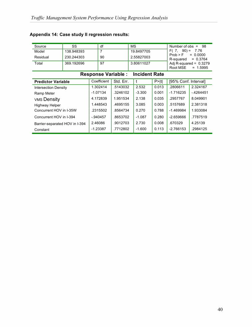
Traffic Management System Performance Using Regression Analysis
40
Appendix 14: Case study II regression results:
Source SS df MS Model 138.948393 7 19.8497705 Residual 230.244303 90 2.55827003
Total 369.192696 97 3.80611027
Number of obs = 98 F( 7, 90) = 7.76 Prob > F = 0.0000 R-squared = 0.3764 Adj R-squared = 0.3279 Root MSE = 1.5995
Response Variable : Incident Rate Predictor Variable Coefficient Std. Err. t P>|t| [95% Conf. Interval] Intersection Density 1.302414 .5143032 2.532 0.013 .2806611 2.324167
Ramp Meter -1.07134 .3246102 -3.300 0.001 -1.716235 -.4264451
VMS Density 4.172839 1.951534 2.138 0.035 .2957767 8.049901
Highway Helper 1.448543 .4695155 3.085 0.003 .5157689 2.381318 Concurrent HOV in I-35W .2315502 .8564734 0.270 0.788 -1.469984 1.933084
Concurrent HOV in I-394 -.940457 .8653702 -1.087 0.280 -2.659666 .7787519
Barrier-separated HOV in I-394 2.46086 .9012703 2.730 0.008 .670329 4.25139
Constant -1.23387 .7712802 -1.600 0.113 -2.766153 .2984125