Traffic Data Collection and Anonymous Vehicle … DATA COLLECTION AND ANONYMOUS VEHICLE ... TRAFFIC...

STATE HIGHWAY ADMINISTRATION

RESEARCH REPORT

TRAFFIC DATA COLLECTION AND ANONYMOUS VEHICLE DETECTION USING WIRELESS SENSOR NETWORKS

FARSHAD AHDI MEHDI KALANTARI KHANDANI

MASOUD HAMEDI ALI HAGHANI

UNIVERSITY OF MARYLAND, COLLEGE PARK

Project number SP009B4H FINAL REPORT

May 2012

MD-12-SP009B4H

Martin O’Malley, Governor

Anthony G. Brown, Lt. Governor

Beverley K. Swaim-Staley, Secretary

Melinda B. Peters, Administrator

2 Introduction

The contents of this report reflect the views of the author who is responsible for the facts and the accuracy of the data presented herein. The contents do not necessarily reflect the official views or policies of the Maryland State Highway Administration. This report does not constitute a standard, specification, or regulation.

3 Introduction

Technical Report Documentation Page 1. Report No.

MD-12-SP009B4H 2. Government Accession No. 3. Recipient's Catalog No.

4. Title and Subtitle

TRAFFIC DATA COLLECTION AND ANONYMOUS VEHICLE

DETECTION USING WIRELESS SENSOR NETWORKS

5. Report Date

6. Performing Organization Code

7. Author/s

FARSHAD AHDI,MEHDI KALANTARI KHANDANI,MASOUD

HAMEDI,ALI HAGHANI

8. Performing Organization Report No.

9. Performing Organization Name and Address

University of Maryland

1179 Glenn L. Martin Hall College Park, MD 20742

10. Work Unit No. (TRAIS)

11. Contract or Grant No.

SP009B4H

12. Sponsoring Organization Name and Address

Maryland State Highway Administration

Office of Policy & Research

707 North Calvert Street

Baltimore MD 21202

13. Type of Report and Period Covered

Final Report

14. Sponsoring Agency Code

(7120) STMD - MDOT/SHA

15. Supplementary Notes

16. Abstract

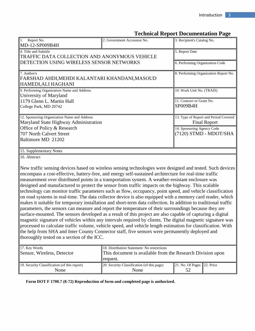
New traffic sensing devices based on wireless sensing technologies were designed and tested. Such devices

encompass a cost-effective, battery-free, and energy self-sustained architecture for real-time traffic

measurement over distributed points in a transportation system. A weather-resistant enclosure was

designed and manufactured to protect the sensor from traffic impacts on the highway. This scalable

technology can monitor traffic parameters such as flow, occupancy, point speed, and vehicle classification

on road systems in real-time. The data collector device is also equipped with a memory card reader, which

makes it suitable for temporary installation and short-term data collection. In addition to traditional traffic

parameters, the sensors can measure and report the temperature of their surroundings because they are

surface-mounted. The sensors developed as a result of this project are also capable of capturing a digital

magnetic signature of vehicles within any intervals required by clients. The digital magnetic signature was

processed to calculate traffic volume, vehicle speed, and vehicle length estimation for classification. With

the help from SHA and Inter County Connector staff, five sensors were permanently deployed and

thoroughly tested on a section of the ICC.

17. Key Words

Sensor, Wireless, Detector 18. Distribution Statement: No restrictions

This document is available from the Research Division upon

request.

19. Security Classification (of this report)

None 20. Security Classification (of this page)

None 21. No. Of Pages

52 22. Price

Form DOT F 1700.7 (8-72) Reproduction of form and completed page is authorized.

4 Introduction

Table of Contents

1. Introduction .............................................................................................................................. 6

2. System Design and Architecture .............................................................................................. 10

2.1. Microcontroller Selection ............................................................................................................ 11

2.2. Energy Harvesting........................................................................................................................ 12

2.3. Enclosure Design ......................................................................................................................... 13

2.4. Roadside Collector ....................................................................................................................... 17

3. Vehicle Detection and Magnetic Signatures ............................................................................. 18

3.1. Magnetic Sensors Principle ......................................................................................................... 19

3.2. Magnetic Signature ..................................................................................................................... 21

3.3. Vehicle Detection and Speed Estimation .................................................................................... 21

3.4. False Detections ............................................................................................................................... 25

4. Test Deployments .................................................................................................................... 27

4.1. System Deployment on the UMD Campus ................................................................................. 27

4.2. Testing Adhesive for Permanent Installation .............................................................................. 28

4.3. Deployment on Inter County Connector (ICC) ........................................................................... 30

5. Signal Processing and Test Results .......................................................................................... 34

5.2. Distributed Data Processing ............................................................................................................. 37

5.3. Speed Measurement ......................................................................................................................... 42

5.4. Length-based Classification ............................................................................................................. 45

5.4. Energy Harvesting ........................................................................................................................... 47

6. Conclusions and Future Research ........................................................................................... 48

7. References ............................................................................................................................... 52

5 Introduction

List of Figures

Figure 1. Traffic Measurement using wireless sensor network............................................................................... 8

Figure 2. Components of the wireless traffic detector device .............................................................................. 11

Figure 3. Protecting the electronic parts using a weather resistant epoxy ........................................................... 13

Figure 4. Housing sensors cast inside a commercial road stud ............................................................................. 14

Figure 5. Initial wireless traffic sensor prototype ................................................................................................ 14

Figure 6. Aluminum version of the initial wireless traffic sensor prototype ......................................................... 15

Figure 7. Wireless traffic sensor in Lexan enclosure ............................................................................................ 16

Figure 8. Enclosure resistance test under real road conditions ............................................................................ 16

Figure 9. Wireless modem for real-time data transmission .................................................................................. 17

Figure 10. Roadside data collection unit .............................................................................................................. 18

Figure 11. Perturbation of Earth’s magnetic field by a ferrous metal vehicle ....................................................... 19

Figure 12. Speed measurement based on magnetic signature collected by two sensors ...................................... 22

Figure 13. Vehicle detection and spot speed estimation experiment ................................................................... 23

Figure 14. Magnetic signature of a vehicle in three direction captured by two sensors ....................................... 24

Figure 15. Analysis of high definition video for ground truth speed measurement .............................................. 25

Figure 16. False detection ................................................................................................................................... 26

Figure 17. Data collection unit with unidirectional antenna deployed on the UMD campus ............................... 28

Figure 18. Testing adhesive and testing installation steps for freeway deployment ............................................ 29

Figure 19. Map of the wireless sensor deployment on the Inter County Connector highway .............................. 30

Figure 20. Arrangement of the wireless sensors on Inter County Connector test site ......................................... 31

Figure 21. Measuring and marking the location of sensors for installation ......................................................... 31

Figure 22. Installing wireless traffic sensors on the Inter County Connector pavement....................................... 32

Figure 23. Test segment of the Inter County Connector after sensor installation ................................................ 33

Figure 24. Roadside data collector installation on Inter County Connector test site ............................................ 34

Figure 25. Sample of magnetic signature signal processing and detection results ............................................... 37

Figure 26. Length of the digital signature signal for a sample time interval ......................................................... 38

Figure 27. Details of the digital signature signal for a seven-minute interval ...................................................... 39

Figure 28. Lane volume data extracted from the digital signature ...................................................................... 39

Figure 29. Sample volume data reported by one senor for different days of the week ....................................... 40

Figure 30. Lane-by-lane comparison of traffic volume ........................................................................................ 41

Figure 31. Signature offset measurement between two consecutive sensors ..................................................... 43

Figure 32. Signature offset measurement for speed estimation .......................................................................... 44

Figure 33. Signature matching for length based classification ............................................................................. 46

Figure 34. Event-matching and signature-processing for vehicle length estimation ............................................ 47

Figure 35. Voltage level of a sensor in a sample day ........................................................................................... 48

6 Introduction

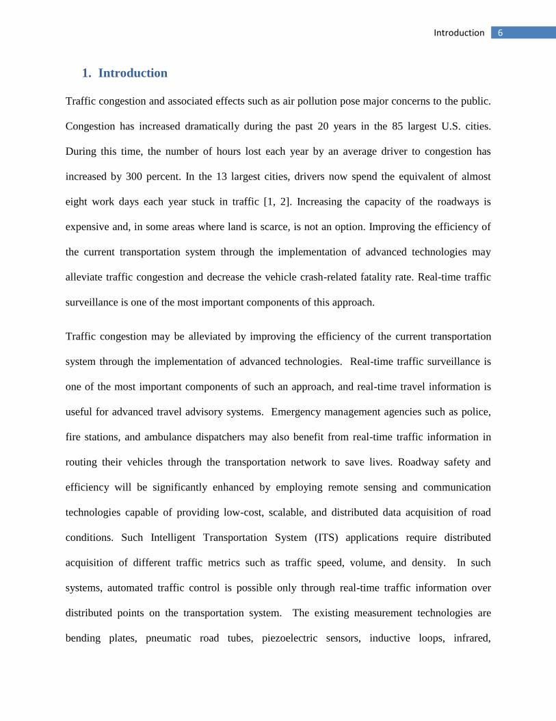
1. Introduction

Traffic congestion and associated effects such as air pollution pose major concerns to the public.

Congestion has increased dramatically during the past 20 years in the 85 largest U.S. cities.

During this time, the number of hours lost each year by an average driver to congestion has

increased by 300 percent. In the 13 largest cities, drivers now spend the equivalent of almost

eight work days each year stuck in traffic [1, 2]. Increasing the capacity of the roadways is

expensive and, in some areas where land is scarce, is not an option. Improving the efficiency of

the current transportation system through the implementation of advanced technologies may

alleviate traffic congestion and decrease the vehicle crash-related fatality rate. Real-time traffic

surveillance is one of the most important components of this approach.

Traffic congestion may be alleviated by improving the efficiency of the current transportation

system through the implementation of advanced technologies. Real-time traffic surveillance is

one of the most important components of such an approach, and real-time travel information is

useful for advanced travel advisory systems. Emergency management agencies such as police,

fire stations, and ambulance dispatchers may also benefit from real-time traffic information in

routing their vehicles through the transportation network to save lives. Roadway safety and

efficiency will be significantly enhanced by employing remote sensing and communication

technologies capable of providing low-cost, scalable, and distributed data acquisition of road

conditions. Such Intelligent Transportation System (ITS) applications require distributed

acquisition of different traffic metrics such as traffic speed, volume, and density. In such

systems, automated traffic control is possible only through real-time traffic information over

distributed points on the transportation system. The existing measurement technologies are

bending plates, pneumatic road tubes, piezoelectric sensors, inductive loops, infrared,

7 Introduction

microwave-doppler/radar, passive acoustic, video image detection, and Bluetooth devices. The

existing data acquisition technologies in transportation systems suffer from the following

drawbacks:

Energy efficiency: Most of the existing technologies need to be constantly connected to

a main power source or battery. Connection to the main power source limits deployment

of the instruments, and using batteries imposes regular maintenance cycles [3].

High cost: The majority of technologies require expensive instruments, which inhibit

cost effectiveness of large-scale and distributed traffic measurements.

Installation and maintenance: Most existing technologies need significant maintenance

and calibration and are costly to install. Installation costs may include wiring of the

instruments to power sources or the wiring required for communication.

Scalability: The majority of existing technologies cannot be deployed on a large scale

due to limitations such as installation cost, wiring, availability of energy sources, etc.

Low-speed and offline measurements: The lack of low-cost real-time communication

between measurement points and the decision-making centers inhibits fast and automated

decision making.

The main goal of this project was to develop an inexpensive and scalable wireless sensor

network prototype, which encompasses a cost-effective architecture for real-time traffic

measurement over distributed points on a transportation system. Energy is one of the main

challenges of a large-scale deployment of sensors. A possible solution is to design sensors that

harvest the needed energy from ambient vibration or from the sun. The sensors use ultra-low

power complementary metal oxide semiconductor (CMOS) technologies, which make the

communications devices extremely energy efficient. The sensors are capable of performing

8 Introduction

simple sensing operations such as traffic count measurement. And, by means of low-range radio

transmissions, the devices form a wireless mesh network. The sensors are able to obtain their

required energy from the vibration in the road surface and added solar sensors, and, therefore, do

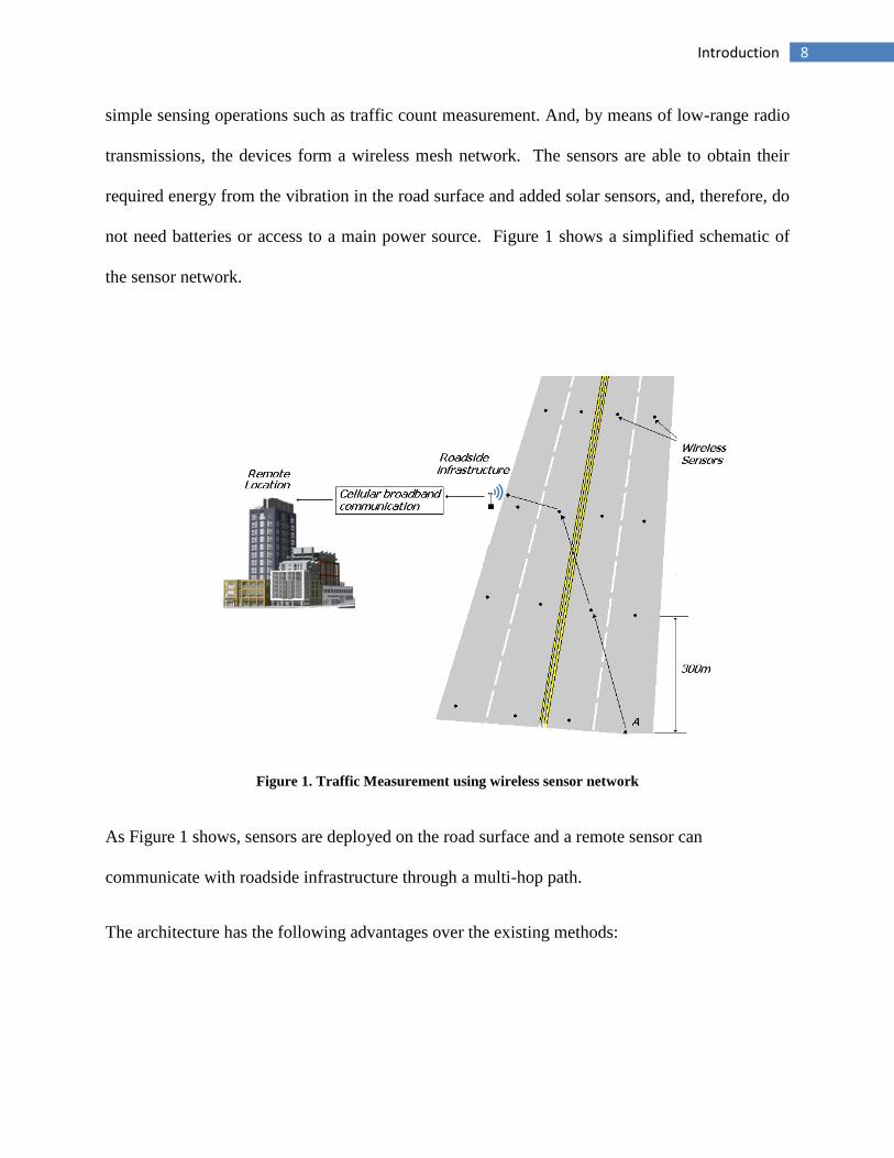
not need batteries or access to a main power source. Figure 1 shows a simplified schematic of

the sensor network.

Figure 1. Traffic Measurement using wireless sensor network

As Figure 1 shows, sensors are deployed on the road surface and a remote sensor can

communicate with roadside infrastructure through a multi-hop path.

The architecture has the following advantages over the existing methods:

9 Introduction

Energy efficiency: The sensing and measurement architecture uses a minimal level of

energy and uses state-of-the-art low-power sensing, amplification, and communication

technologies.

Broad range of measurement: With the sensor networking architecture, several types of

traffic measurements can be performed. Examples of some measurements include: Traffic

volume and density, traffic speed, classification of vehicle types (e.g., based on length).

Furthermore, with a larger density, the sensors can provide an end-to-end communication

medium.

Ease of installation: Compared to existing systems, the system requires minimal installation

effort. For each traffic measurement point, the system requires a roadside data collection

point and installing a few wireless sensors on the road surface. Because sensors are both

small and wireless, lane closure time and traffic disturbance for the installation is minimal

and not labor intensive.

Endurance: Since the sensors do not require batteries, calibration, or any other type of

maintenance after installation, the system has a very long life expectancy.

Low maintenance requirements: Because the measurement devices do not need wiring or

batteries, their maintenance demand is minimal.

The developed sensor architecture is specific to ITS applications where energy harvesting makes

the best use of both vibration energy from the road surfaces and solar energy. Also, the wireless

sensors are equipped with the necessary instrumentation components such as anisotropic

magnetoresistance elements for the purpose of detecting vehicles.

10 System Design and Architecture

2. System Design and Architecture

The traffic detection devices developed in this project harvest their required energy from their

environment to power up the sensing element and telecommunication modules and, thus, do not

need batteries. The sensing part uses magnetic sensors for detecting vehicles and the

communication is wireless. In summary each device includes the following components (Figure

2):

Sensing elements: The main sensing element is a magnetic sensor that generates a digital

signature of a passing vehicle based on disturbance of the magnetic field caused by the

ferromagnetic material of the vehicle.

Solar panel: A small, thin solar panel is placed on the top section of the devices and is

protected by a heavy-duty transparent fiber glass casing to turn ambient light energy into

electricity.

Super capacitor: This part is an environmentally friendly capacitive media for storing

harvested energy from solar and vibration sources.

Circuit and antenna: This component includes a communication antenna and the

necessary circuits for wake-up scheduling, instrumentation, amplification, and

communication.

All the above components are integrated into a custom designed snow plow-safe casing with

an overall thickness of about 0.5 inches. An electronics-friendly silicon sealant makes the

devices weather resistant. Deployment is done on the road surface using adhesive materials.

The following sections describe the technical details.


Figure 2. Components of the wireless traffic detector device

2.1. Microcontroller Selection

Finding an appropriate microcontroller that supports wireless communication and that is energy

efficient and fast enough to handle the magnetic sensor is crucial. Based on past experience, the

research team targeted and extensively tested two microcontrollers during the design phase.

These included the Peripheral Interface Controller (PIC) and Texas Instrument-based

microcontrollers.

After some preliminary investigation, Texas Instrument (TI) microcontroller CC2430 was

selected. This chip represents the Chipcon’s second-generation ZigBee-compliant platform. It is

a System-on-Chip (SoC) solution that combines the industry-leading radio 2.4 GHz transceiver

of the IEEE 802.15.4-compliant CC2420 with an industry-proven, compact, and efficient 8051

microcontroller.

The family of CC2430 microcontrollers comes in three products: CC2430-F32, CC2430-F64,

and CC2430-F128. The main difference between these chips is the amount of flash memory on

board, which are 32, 64 and 128 KB with 8 KB of RAM. The CC2430 family uses Chipcon's

SmartRF®03 technology platform and is designed in 0.18 micrometer CMOS, available in a

small 7 x 7 mm, 48-pin package. One of the most important advantages of these chips are their


energy efficiency. In reception and transmission modes, the microcontrollers consume

approximately 27 mA and 25 mA, respectively. In sleep mode, the CC2430 microcontrollers

consume 7uA. Because of the ultra-low power consumption in sleep mode, small battery can

sustain the chips for several years. These chips can be programmed for any ZigBee wireless

node, including coordinators, routers, and end devices. Most importantly, the protocol stack (Z-

Stack) is provided by Texas Instruments, which makes the development period considerably

shorter.

In the middle of this project, a new version of this chip was introduced, the CC2530. The new

chip provides a larger flash memory (up to 256 KB), which makes it suitable for ZigBee PRO

applications. The larger memory size of this chip allows for on-chip, over-the-air-download to

support in-system reprogramming. As a result, the microcontroller used in the prototype devices

was replaced with CC2530 to build the new version of the hardware. Necessary modification in

the embedded code accommodated the updated features.

2.2. Energy Harvesting

The traffic sensors are energetically self-sufficient and, therefore, environmentally friendly. In

addition to reducing the energy consumption, the required energy is harvested from the

environment. This project used solar panels. Although ambient light is a good source of energy,

it fluctuates with the time of the day, weather conditions, and the season (days are shorter in the

winter and longer in summer). Thus, the energy-harvesting component has to account for these

factors. To keep the sensors functioning without sunlight, energy must be stored during the day.

Several brands and types of solar panels were performance tested in order to select appropriate

components. The solar panel was protected by applying clear resin in the final design.


2.3. Enclosure Design

In order to deploy prototype sensors for conducting experiments in traffic, an appropriate

enclosure is needed to protect the devices against harsh road conditions. Instead of designing a

customized case, commercially available road studs were adopted. To develop a housing for the

electronic parts, necessary modifications were made to the cases in the University of Maryland

machine shop.

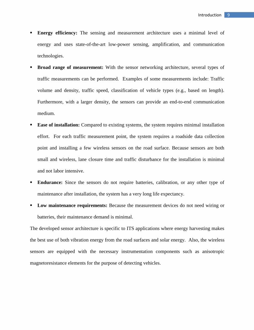
Another important consideration was to protect devices against humidity and rain. EasyCast, a

product from TAP Plastics, made the devices waterproof. Additionally, several TAP Plastics

molds were used to cast the resin in proper shapes. Figure 3 shows examples of a round shape

casting on the left and a surface mount rectangular shape on the right.

Figure 3. Protecting the electronic parts using a weather resistant epoxy

To protect the devices against the weight of a vehicle, commercial road studs were modified to

accommodate casted electronic parts (Figure 4).


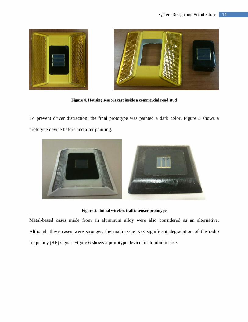
Figure 4. Housing sensors cast inside a commercial road stud

To prevent driver distraction, the final prototype was painted a dark color. Figure 5 shows a

prototype device before and after painting.

Figure 5. Initial wireless traffic sensor prototype

In

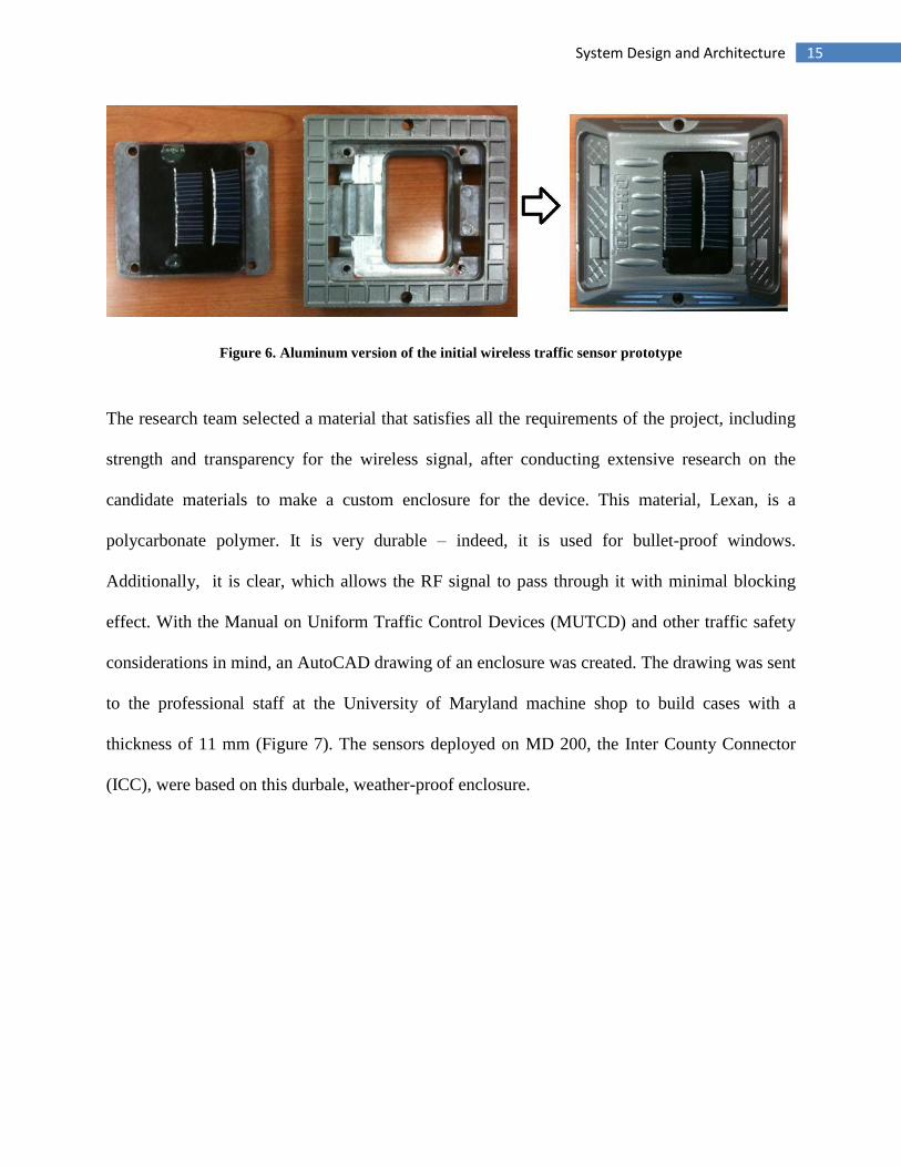
Metal-based cases made from an aluminum alloy were also considered as an alternative.

Although these cases were stronger, the main issue was significant degradation of the radio

frequency (RF) signal. Figure 6 shows a prototype device in aluminum case.


Figure 6. Aluminum version of the initial wireless traffic sensor prototype

The research team selected a material that satisfies all the requirements of the project, including

strength and transparency for the wireless signal, after conducting extensive research on the

candidate materials to make a custom enclosure for the device. This material, Lexan, is a

polycarbonate polymer. It is very durable – indeed, it is used for bullet-proof windows.

Additionally, it is clear, which allows the RF signal to pass through it with minimal blocking

effect. With the Manual on Uniform Traffic Control Devices (MUTCD) and other traffic safety

considerations in mind, an AutoCAD drawing of an enclosure was created. The drawing was sent

to the professional staff at the University of Maryland machine shop to build cases with a

thickness of 11 mm (Figure 7). The sensors deployed on MD 200, the Inter County Connector

(ICC), were based on this durbale, weather-proof enclosure.


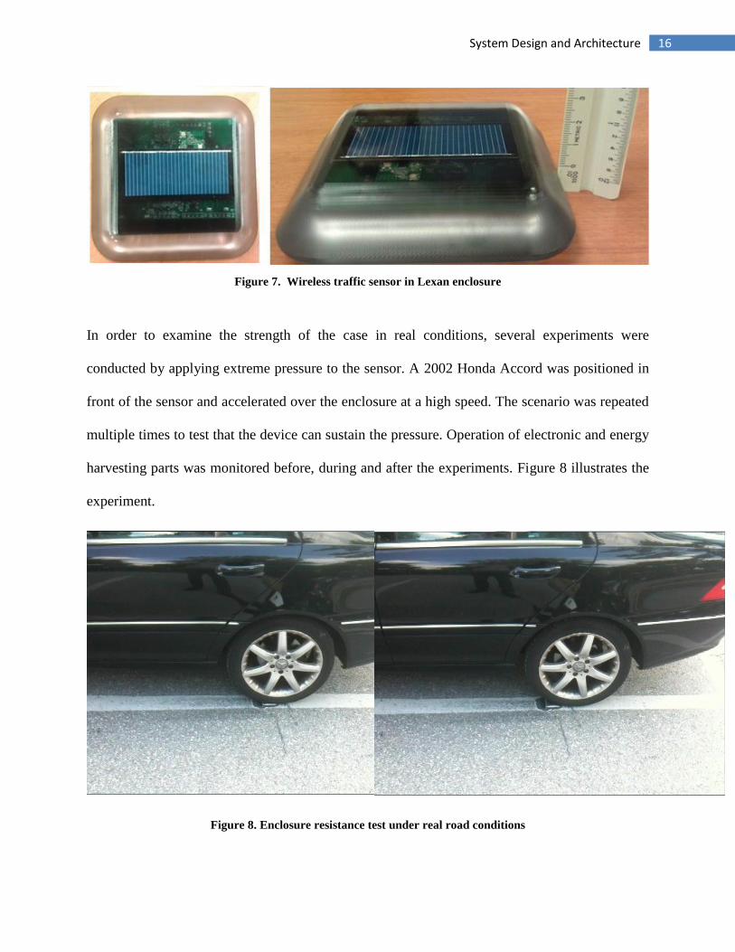
Figure 7. Wireless traffic sensor in Lexan enclosure

In order to examine the strength of the case in real conditions, several experiments were

conducted by applying extreme pressure to the sensor. A 2002 Honda Accord was positioned in

front of the sensor and accelerated over the enclosure at a high speed. The scenario was repeated

multiple times to test that the device can sustain the pressure. Operation of electronic and energy

harvesting parts was monitored before, during and after the experiments. Figure 8 illustrates the

experiment.

Figure 8. Enclosure resistance test under real road conditions


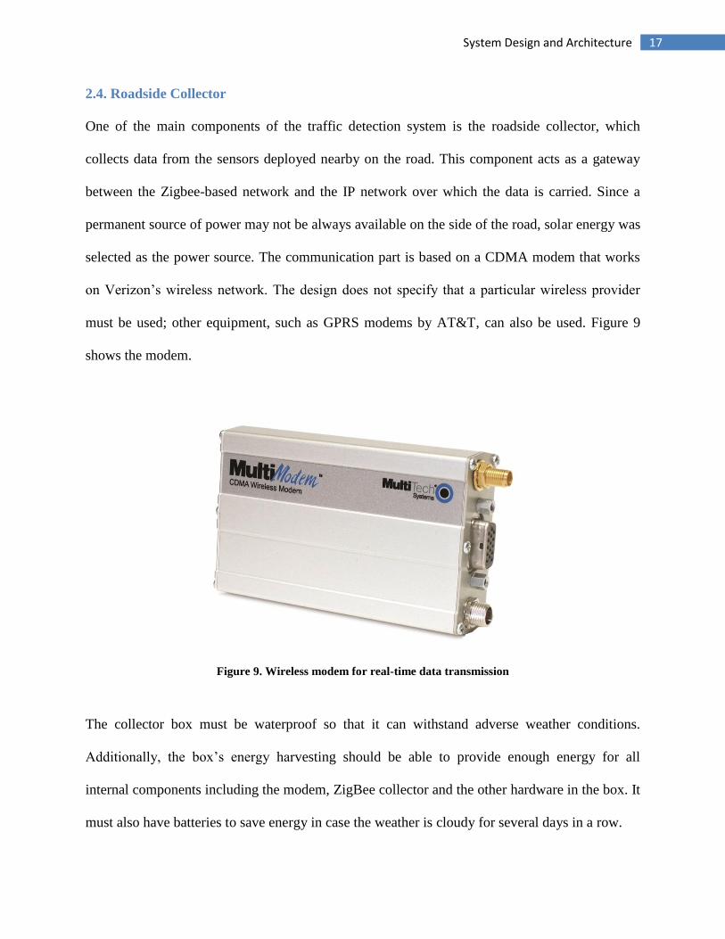
2.4. Roadside Collector

One of the main components of the traffic detection system is the roadside collector, which

collects data from the sensors deployed nearby on the road. This component acts as a gateway

between the Zigbee-based network and the IP network over which the data is carried. Since a

permanent source of power may not be always available on the side of the road, solar energy was

selected as the power source. The communication part is based on a CDMA modem that works

on Verizon’s wireless network. The design does not specify that a particular wireless provider

must be used; other equipment, such as GPRS modems by AT&T, can also be used. Figure 9

shows the modem.

Figure 9. Wireless modem for real-time data transmission

The collector box must be waterproof so that it can withstand adverse weather conditions.

Additionally, the box’s energy harvesting should be able to provide enough energy for all

internal components including the modem, ZigBee collector and the other hardware in the box. It

must also have batteries to save energy in case the weather is cloudy for several days in a row.

18 Vehicle Detection and Magnetic Signatures

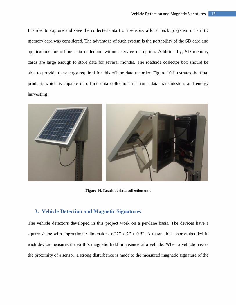
In order to capture and save the collected data from sensors, a local backup system on an SD

memory card was considered. The advantage of such system is the portability of the SD card and

applications for offline data collection without service disruption. Additionally, SD memory

cards are large enough to store data for several months. The roadside collector box should be

able to provide the energy required for this offline data recorder. Figure 10 illustrates the final

product, which is capable of offline data collection, real-time data transmission, and energy

harvesting

Figure 10. Roadside data collection unit

3. Vehicle Detection and Magnetic Signatures

The vehicle detectors developed in this project work on a per-lane basis. The devices have a

square shape with approximate dimensions of 2” x 2” x 0.5”. A magnetic sensor embedded in

each device measures the earth’s magnetic field in absence of a vehicle. When a vehicle passes

the proximity of a sensor, a strong disturbance is made to the measured magnetic signature of the


vehicle due to the large mass of steel and other ferromagnetic material in the vehicles. The

signature is collected in three dimensions, each of which has a wave form.

3.1. Magnetic Sensors Principle

Magnetic sensors detect a vehicle’s signature by measuring the change in the magnetic lines of

flux caused by the change in field values produced by a moving ferrous metal vehicle (Figure

11). There are two types of sensors that can be used for vehicle detection using magnetic field

measurement: Anisotropic magneto-resistive (AMR) sensors and giant magneto-resistive (GMR)

sensors. AMR sensors are directional sensors and can provide only an amplitude response to

magnetic fields in their sensitive axis. Multi-axis AMR sensors can be made by combining the

measurement of multiple one-axis sensors [4]. GMR sensors can also be used for low magnetic

field sensing. These kinds of sensors have a broad sensitivity to amplitudes with little

directionality.

Figure 11. Perturbation of Earth’s magnetic field by a ferrous metal vehicle

The main difference between AMR and GMR sensors is their linearity. Whereas AMR sensors’

response to the change in the magnetic field is linear, the same is not true for GMR sensors. In


order to use GMR sensors for detecting vehicles, its response must be linearized using a nearby

magnetic bias field. This linearizing can be achieved through either a permanent magnet or a

direct current-driven solenoid to gain improved linearity.

In this project, the performance of both AMR and GMR sensors was evaluated. The first design

was based on the GMR sensors. Experiments were carried out in which the type of vehicle and

its orientation were changed. The GMR sensors were capable of detecting a passing vehicle in all

conditions. However, non-linearity of the sensors was an issue. External magnetic bias was used

to linearize the sensors as much as possible; however, non-identical magnetic bias complicated

the sensor calibration. In other words, the linearization process was complex and low

performing.

The AMR sensors consist of magneto-resistive elements oriented on a wheatstone bridge; the

resistance of magneto-resistive elements change when exposed to a magnetic field. These

elements are made of permalloy thin films that achieve a resistance of approximately 1000 ohms.

In the absence of any magnetic field, the values of the elements are matched within one ohm of

each other. In the resulting bridge, the opposite elements are identical.

One of the challenges of using magnetic sensors is the effect of Earth’s magnetic field. The

readout signals from the sensors change with the orientation of the installed sensors on the road

because Earth’s magnetic field intensity changes in different directions. To mitigate this issue, an

adaptive gain amplifier was used.


3.2. Magnetic Signature

Earth’s magnetic field provides a baseline for magnetic fields that is relatively constant with a

fixed sensor installation. A nominal value for Earth’s magnetic field strength is approximately

0.5 gauss, so the readout of each axis ranges 0.0 gauss ± 0.7 gauss. Once vehicles come into

proximity of the sensor, the level of magnetic field varies depending on the mass of the ferrous

materials in the body of the vehicle. (It should be noted that vehicles’ bodies consists of both

soft- and hard-iron materials because the two types of iron have different effects on magnetic

flux. Soft iron concentrates magnetic flux into the material and does not have any remnant flux

generated within the material. Hard iron, on the other hand, causes flux concentration as well as

remnant flux generation. (Flux density is in the order of hundreds of gauss and the remnant flux

caused by hard iron is less than ± 2 gauss.)

The concentration of Earth’s magnetic flux caused by soft irons will generally increase the flux

amplitude. This increment is usually less than half of the residual bias value at the sensor

location. As a result, the magnetic sensors should see a few tens to hundreds of milligauss of

Earth field bias, with up to ± 3 gauss of spikes. The vehicle detection system in this project

mostly deals with the level of change of the magnetic field instead of dynamic peaks generated

by the vehicle.

3.3. Vehicle Detection and Speed Estimation

Installing two detectors in one lane that are separated by a predetermined distance in the

direction of traffic allows for the measurement of vehicles’ speed based on the signature’s time

difference. After finding the speed of a vehicle, its length can be estimated.


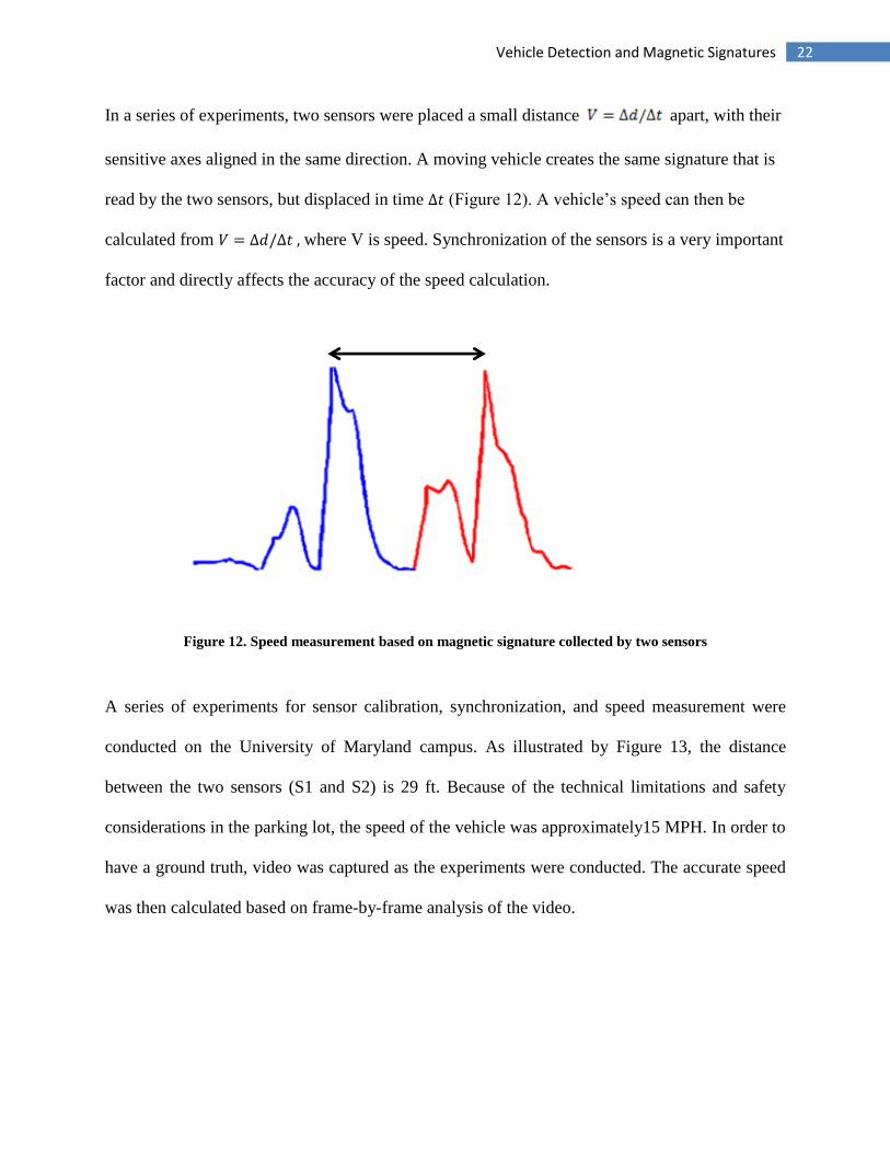
In a series of experiments, two sensors were placed a small distance apart, with their

sensitive axes aligned in the same direction. A moving vehicle creates the same signature that is

read by the two sensors, but displaced in time (Figure 12). A vehicle’s speed can then be

calculated from where V is speed. Synchronization of the sensors is a very important

factor and directly affects the accuracy of the speed calculation.

Figure 12. Speed measurement based on magnetic signature collected by two sensors

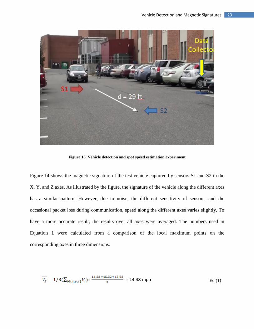
A series of experiments for sensor calibration, synchronization, and speed measurement were

conducted on the University of Maryland campus. As illustrated by Figure 13, the distance

between the two sensors (S1 and S2) is 29 ft. Because of the technical limitations and safety

considerations in the parking lot, the speed of the vehicle was approximately15 MPH. In order to

have a ground truth, video was captured as the experiments were conducted. The accurate speed

was then calculated based on frame-by-frame analysis of the video.


Figure 13. Vehicle detection and spot speed estimation experiment

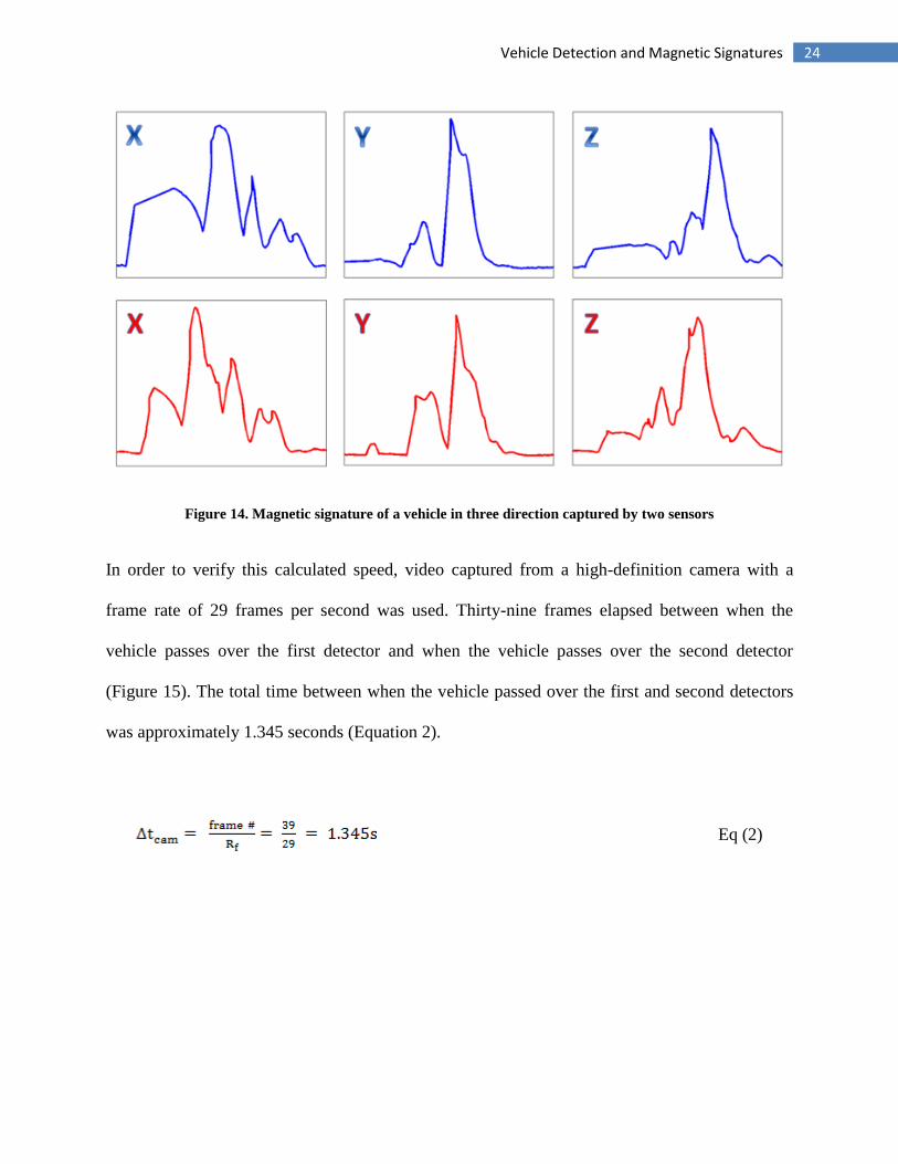
Figure 14 shows the magnetic signature of the test vehicle captured by sensors S1 and S2 in the

X, Y, and Z axes. As illustrated by the figure, the signature of the vehicle along the different axes

has a similar pattern. However, due to noise, the different sensitivity of sensors, and the

occasional packet loss during communication, speed along the different axes varies slightly. To

have a more accurate result, the results over all axes were averaged. The numbers used in

Equation 1 were calculated from a comparison of the local maximum points on the

corresponding axes in three dimensions.

Eq (1)

= = 14.48 mph


Figure 14. Magnetic signature of a vehicle in three direction captured by two sensors

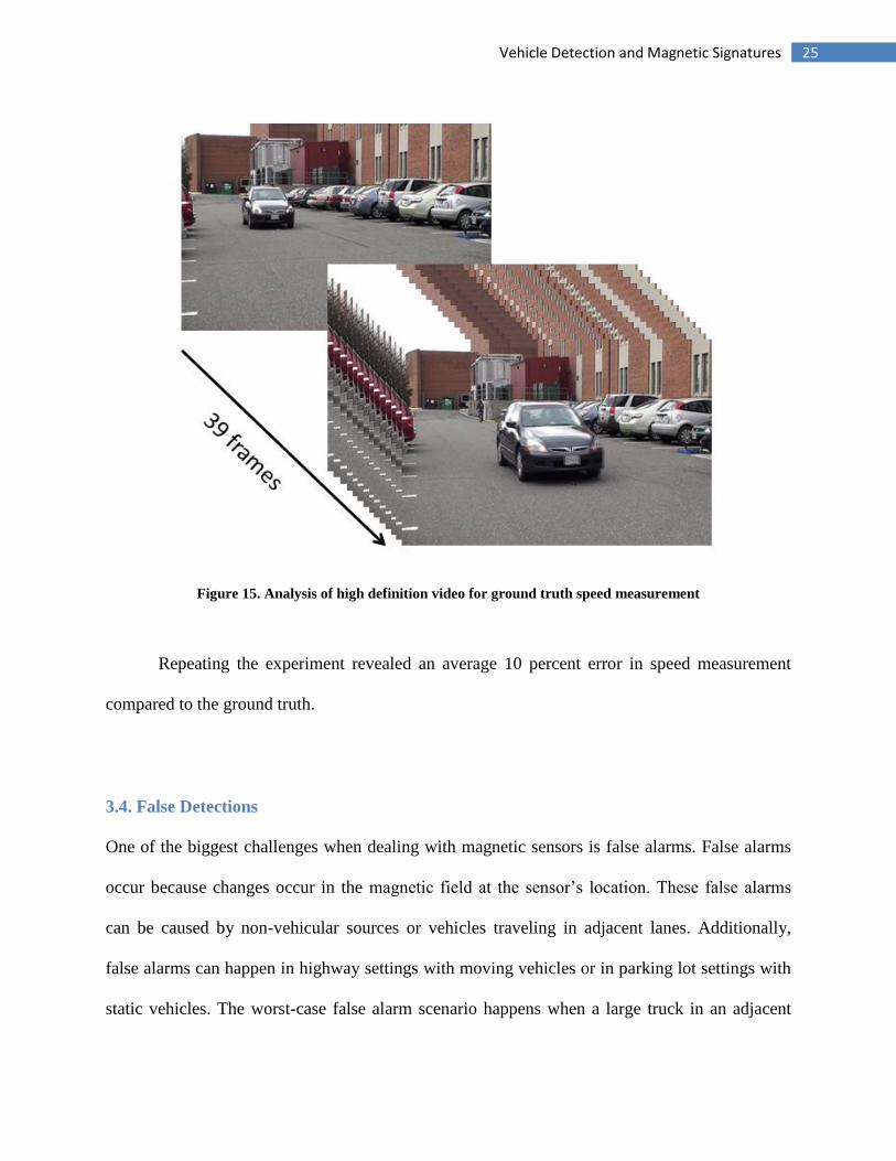
In order to verify this calculated speed, video captured from a high-definition camera with a

frame rate of 29 frames per second was used. Thirty-nine frames elapsed between when the

vehicle passes over the first detector and when the vehicle passes over the second detector

(Figure 15). The total time between when the vehicle passed over the first and second detectors

was approximately 1.345 seconds (Equation 2).

Eq (2)


Figure 15. Analysis of high definition video for ground truth speed measurement

Repeating the experiment revealed an average 10 percent error in speed measurement

compared to the ground truth.

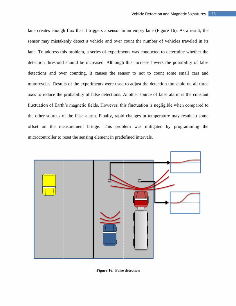
3.4. False Detections

One of the biggest challenges when dealing with magnetic sensors is false alarms. False alarms

occur because changes occur in the magnetic field at the sensor’s location. These false alarms

can be caused by non-vehicular sources or vehicles traveling in adjacent lanes. Additionally,

false alarms can happen in highway settings with moving vehicles or in parking lot settings with

static vehicles. The worst-case false alarm scenario happens when a large truck in an adjacent


lane creates enough flux that it triggers a sensor in an empty lane (Figure 16). As a result, the

sensor may mistakenly detect a vehicle and over count the number of vehicles traveled in its

lane. To address this problem, a series of experiments was conducted to determine whether the

detection threshold should be increased. Although this increase lowers the possibility of false

detections and over counting, it causes the sensor to not to count some small cars and

motorcycles. Results of the experiments were used to adjust the detection threshold on all three

axes to reduce the probability of false detections. Another source of false alarm is the constant

fluctuation of Earth’s magnetic fields. However, this fluctuation is negligible when compared to

the other sources of the false alarm. Finally, rapid changes in temperature may result in some

offset on the measurement bridge. This problem was mitigated by programming the

microcontroller to reset the sensing element in predefined intervals.

Figure 16. False detection

27 Test Deployments

4. Test Deployments

The goal of this project was to develop prototypes that work in a real traffic environment and not

just in a lab. After designing and building the enclosure, several devices were deployed and

tested on the University of Maryland campus and a highway.

4.1. System Deployment on the UMD Campus

Multiple experiments were first conducted on UMD campus roads before highway deployment

and testing of the devices. The results were used to improve the sensors and the roadside

collector. To analyze the signal reception for the collector, the collector unit was installed on the

roof of the four-story engineering building; the accompanying sensors were deployed on Campus

Drive, which runs in front of the building. This configuration allowed us to test the

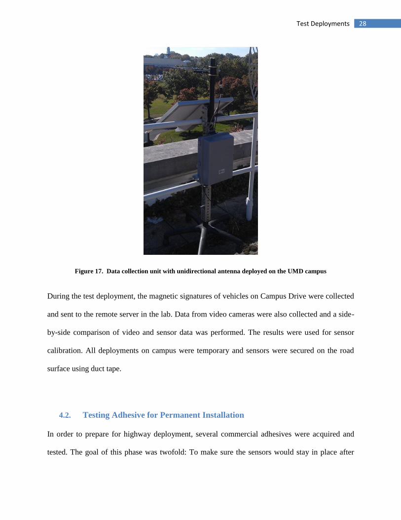
communication range and the energy harvesting abilities of the sensors and the collector. Figure

17 shows testing the data collection unit with a unidirectional antenna on top of the engineering

building; Campus Drive can be seen just below the solar panel.

28 Test Deployments

Figure 17. Data collection unit with unidirectional antenna deployed on the UMD campus

During the test deployment, the magnetic signatures of vehicles on Campus Drive were collected

and sent to the remote server in the lab. Data from video cameras were also collected and a side-

by-side comparison of video and sensor data was performed. The results were used for sensor

calibration. All deployments on campus were temporary and sensors were secured on the road

surface using duct tape.

4.2. Testing Adhesive for Permanent Installation

In order to prepare for highway deployment, several commercial adhesives were acquired and

tested. The goal of this phase was twofold: To make sure the sensors would stay in place after

29 Test Deployments

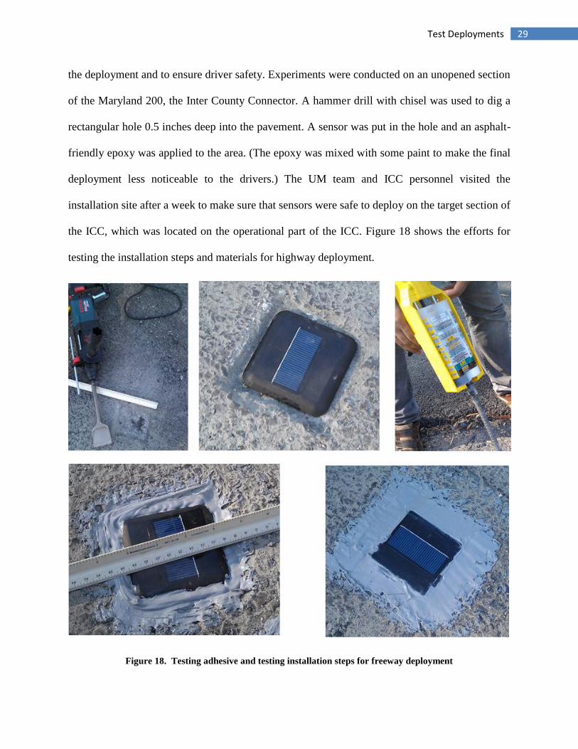
the deployment and to ensure driver safety. Experiments were conducted on an unopened section

of the Maryland 200, the Inter County Connector. A hammer drill with chisel was used to dig a

rectangular hole 0.5 inches deep into the pavement. A sensor was put in the hole and an asphalt-

friendly epoxy was applied to the area. (The epoxy was mixed with some paint to make the final

deployment less noticeable to the drivers.) The UM team and ICC personnel visited the

installation site after a week to make sure that sensors were safe to deploy on the target section of

the ICC, which was located on the operational part of the ICC. Figure 18 shows the efforts for

testing the installation steps and materials for highway deployment.

Figure 18. Testing adhesive and testing installation steps for freeway deployment

30 Test Deployments

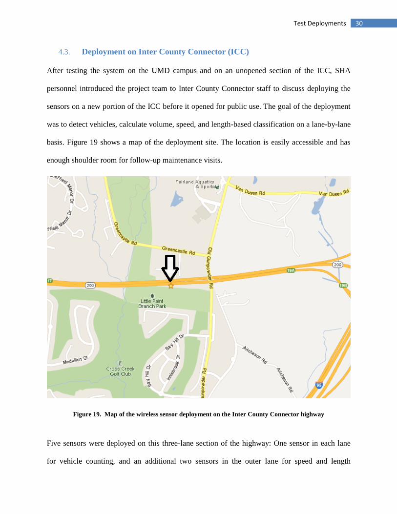
4.3. Deployment on Inter County Connector (ICC)

After testing the system on the UMD campus and on an unopened section of the ICC, SHA

personnel introduced the project team to Inter County Connector staff to discuss deploying the

sensors on a new portion of the ICC before it opened for public use. The goal of the deployment

was to detect vehicles, calculate volume, speed, and length-based classification on a lane-by-lane

basis. Figure 19 shows a map of the deployment site. The location is easily accessible and has

enough shoulder room for follow-up maintenance visits.

Figure 19. Map of the wireless sensor deployment on the Inter County Connector highway

Five sensors were deployed on this three-lane section of the highway: One sensor in each lane

for vehicle counting, and an additional two sensors in the outer lane for speed and length

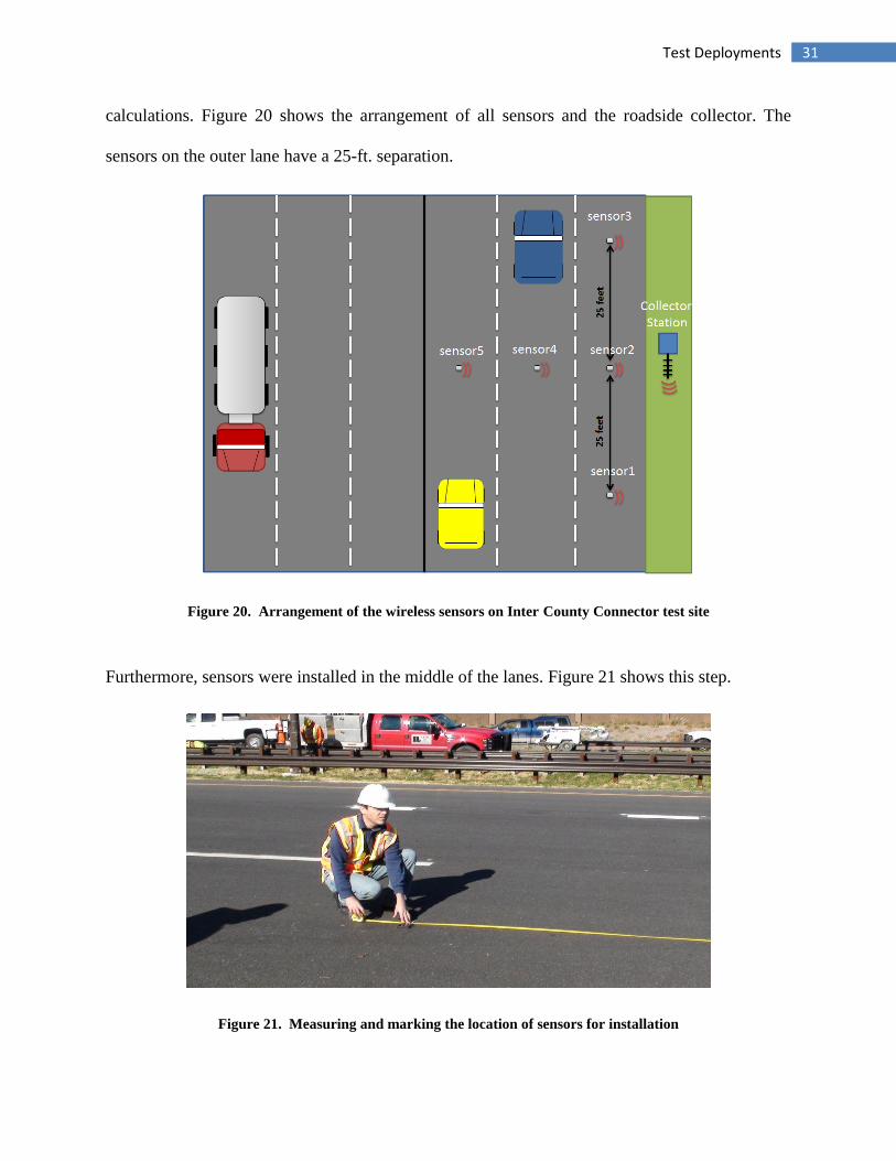
31 Test Deployments

calculations. Figure 20 shows the arrangement of all sensors and the roadside collector. The

sensors on the outer lane have a 25-ft. separation.

Figure 20. Arrangement of the wireless sensors on Inter County Connector test site

Furthermore, sensors were installed in the middle of the lanes. Figure 21 shows this step.

Figure 21. Measuring and marking the location of sensors for installation

32 Test Deployments

After marking the location of the sensors, each sensor was carefully installed using the same

procedure described in section 4.2. Figure 22 shows the installation steps. (Blue tape was used to

avoid making cosmetic damage to the pavement after applying the epoxy.)

Figure 22. Installing wireless traffic sensors on the Inter County Connector pavement

After removing the tapes only the solar panel window of the senor remained exposed for energy

harvesting. It should be noted that sand was applied to the surface of the sensor to prevent it from

reflecting sunlight to the driver’s eyes. Additionally it improves the performance of the solar

panel by attracting more light. As a result of this procedure, the sensors are barely noticeable on

the road. Figure 23 shows the final results after installation.

33 Test Deployments

Figure 23. Test segment of the Inter County Connector after sensor installation

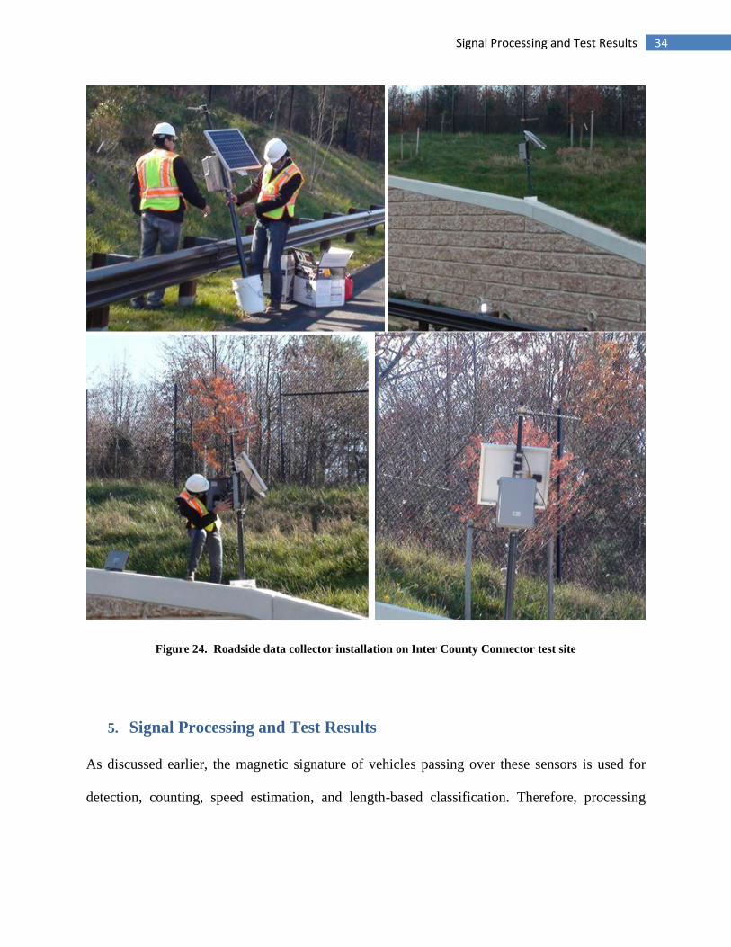
After deploying sensors on the ICC, an appropriate location for the roadside collector was

identified on an uphill next to the road. The roadside collector was mounted on a metal pole and

was secured in a heavy bucket. The roadside collector and the mount were secured to the wall

using metal ties. Figure 24 shows the installation and calibration of the unit. The roadside

collector was set up to send the data to a remote server on UMD’s campus. As discussed earlier,

the collector also has the capability to save a copy of the collected data on an SD memory card in

the unlikely event that the communication link fails.

34 Signal Processing and Test Results

Figure 24. Roadside data collector installation on Inter County Connector test site

5. Signal Processing and Test Results

As discussed earlier, the magnetic signature of vehicles passing over these sensors is used for

detection, counting, speed estimation, and length-based classification. Therefore, processing


vehicle signature data in order to convert them to volume, speed, and other information is a

crucial task.

Upon capturing the raw data, the microcontroller processes the data for information extraction.

Specifically, the noise must be separated from data in this process. Additionally, there is a low-

frequency offset in the data that must be eliminated because of the offset of the sensors, and the

effects of temperature drift and Earth’s magnetic field.

The data can be processed either in a distributed scheme (i.e., within individual sensors) or in a

centralized scheme (i.e., in a server). Each method has advantages and disadvantages.

Distributed data processing has much lower data transmission, which results in significant

energy savings. This is especially useful during the intervals during which the traffic rate is low

(such as late evening hours and weekend days). Distributed processing also reduces the amount

of data collected by the server, thus lowering the processing load on the server side. However,

due to the limited low-processing capability of microcontrollers, sophisticated algorithms cannot

be implemented in the sensors. Therefore, in the current deployment uses distributed data

processing.

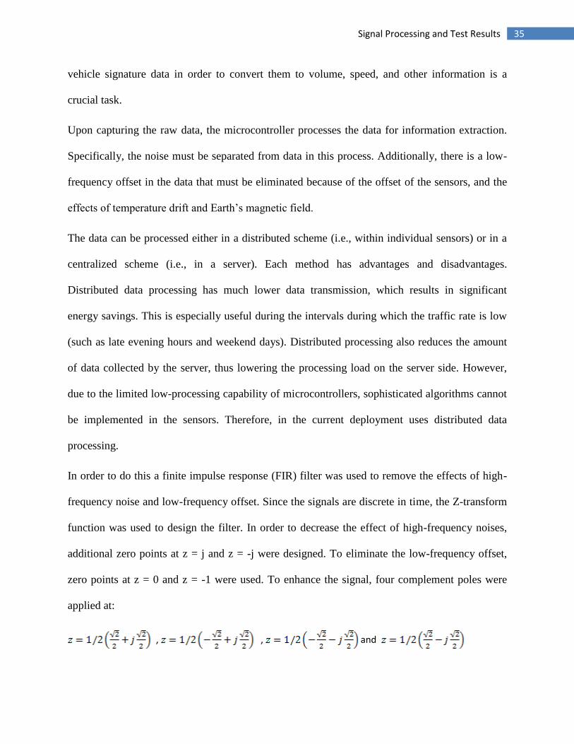
In order to do this a finite impulse response (FIR) filter was used to remove the effects of high-

frequency noise and low-frequency offset. Since the signals are discrete in time, the Z-transform

function was used to design the filter. In order to decrease the effect of high-frequency noises,

additional zero points at z = j and z = -j were designed. To eliminate the low-frequency offset,

zero points at z = 0 and z = -1 were used. To enhance the signal, four complement poles were

applied at:

, , and


As a result, the final Z-transform function is:

= = Eq(3)

Therefore:

Eq(4)

The transformation function in Equation 4 and filtering mechanism were coded in the

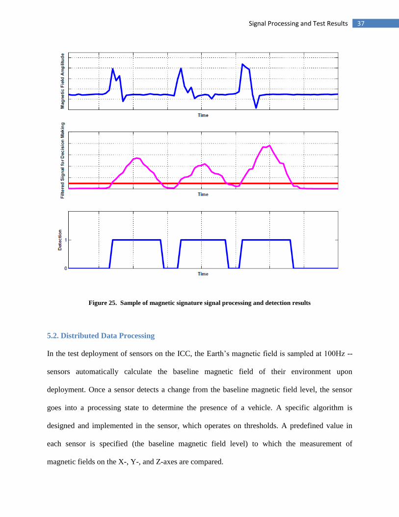
microcontroller. Figure 25 is an example of magnetic signature (top, blue), the processed version

(pink), and the detection signal (bottom, blue). In this figure, the original signal was filtered to

bell curves by eliminating noises and offsets. Then, using a threshold comparison, the sensor can

make a detection on a vehicle above it.


Figure 25. Sample of magnetic signature signal processing and detection results

5.2. Distributed Data Processing

In the test deployment of sensors on the ICC, the Earth’s magnetic field is sampled at 100Hz --

sensors automatically calculate the baseline magnetic field of their environment upon

deployment. Once a sensor detects a change from the baseline magnetic field level, the sensor

goes into a processing state to determine the presence of a vehicle. A specific algorithm is

designed and implemented in the sensor, which operates on thresholds. A predefined value in

each sensor is specified (the baseline magnetic field level) to which the measurement of

magnetic fields on the X-, Y-, and Z-axes are compared.


If a vehicle is detected, the sensor collects data about how long it takes the vehicle to travel over

the sensor. (These times are not directly related to the length of the vehicle – they are also a

factor of the vehicle’s speed. For example, a long vehicle may travel at a high speed. Therefore,

a sensor would collect a short time signature for that vehicle.) In order to have an accurate

estimate of a vehicle’s length, the vehicle’s speed needs to be determined first. Figure 26 depicts

the length of signatures collected during different times of the day by one of the sensors on ICC.

Figure 26. Length of the digital signature signal for a sample time interval

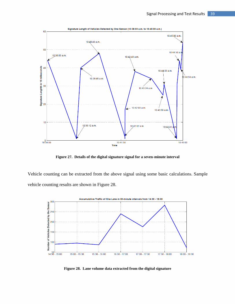
Figure 27 shows a detailed version of the signature length for a seven-minute interval. As noted

in the figure, 14 vehicles passed over the sensor.


Figure 27. Details of the digital signature signal for a seven-minute interval

Vehicle counting can be extracted from the above signal using some basic calculations. Sample

vehicle counting results are shown in Figure 28.

Figure 28. Lane volume data extracted from the digital signature


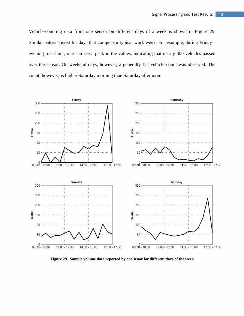
Vehicle-counting data from one sensor on different days of a week is shown in Figure 29.

Similar patterns exist for days that compose a typical work week. For example, during Friday’s

evening rush hour, one can see a peak in the values, indicating that nearly 300 vehicles passed

over the sensor. On weekend days, however, a generally flat vehicle count was observed. The

count, however, is higher Saturday morning than Saturday afternoon.

Figure 29. Sample volume data reported by one senor for different days of the week


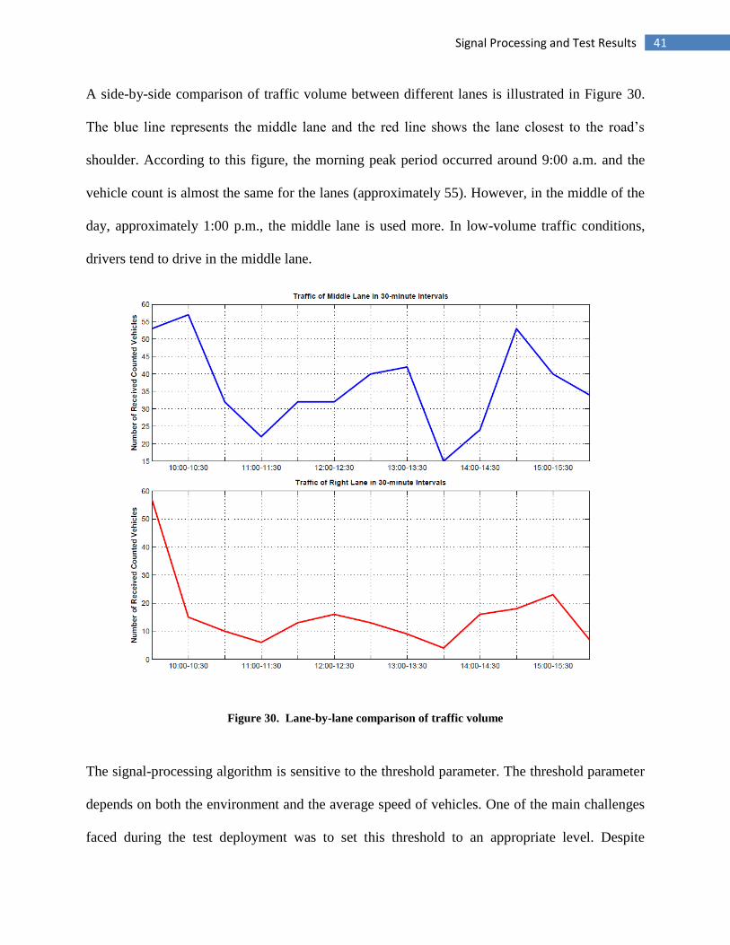
A side-by-side comparison of traffic volume between different lanes is illustrated in Figure 30.

The blue line represents the middle lane and the red line shows the lane closest to the road’s

shoulder. According to this figure, the morning peak period occurred around 9:00 a.m. and the

vehicle count is almost the same for the lanes (approximately 55). However, in the middle of the

day, approximately 1:00 p.m., the middle lane is used more. In low-volume traffic conditions,

drivers tend to drive in the middle lane.

Figure 30. Lane-by-lane comparison of traffic volume

The signal-processing algorithm is sensitive to the threshold parameter. The threshold parameter

depends on both the environment and the average speed of vehicles. One of the main challenges

faced during the test deployment was to set this threshold to an appropriate level. Despite


extensive effort and multiple experiments on UM’s campus, the parameters that resulted from

those trials could not be applied to highway conditions that differed in traffic volume and

number of lanes (Campus Drive has only one lane in each direction). Modifications to these

parameters were necessary to prepare sensors for freeway conditions. Another challenge that the

firmware of the sensors could not be changed after the sensors were deployed, so over-the-air

programming of the devices was not possible after deployment. These challenges were addressed

by programming into sensors a series of threshold levels and by using the most appropriate

parameter after calibration. One advantage of this effort was to analyze the marginal impact of

different threshold values by comparing it to the ground-truth collected by video imaging.

5.3. Speed Measurement

The speed of a vehicle can be determined by using two sensors deployed on the same lane with a

predefined distance between them. (This method assumes that a vehicle does not change lanes in

the 25 ft. between the ICC sensors.) The time offset for the signature of the same vehicle on the

two sensors is used to estimate the speed.

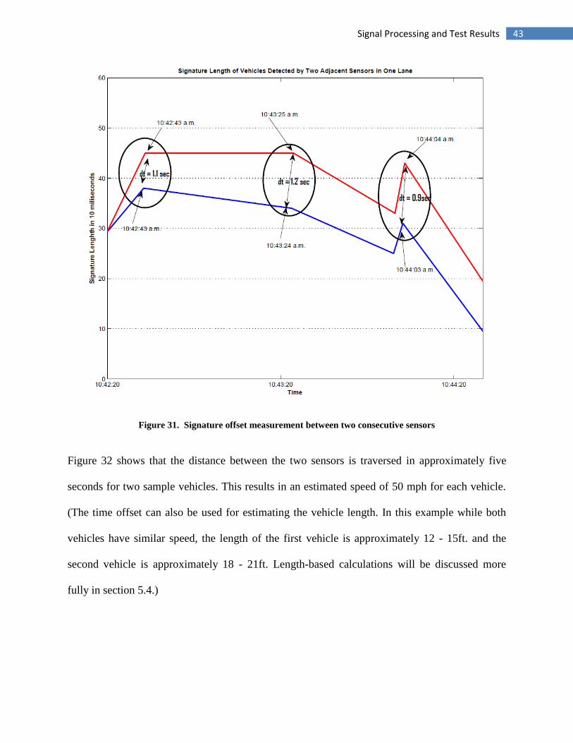
In Figure 31, the red and blue lines show the data from two sensors in one lane. Since there are

three sensors on the rightmost lane of the ICC deployment, the signature time offset can be

matched based on the two farthest sensors, which are approximately 50 ft. apart.


Figure 31. Signature offset measurement between two consecutive sensors

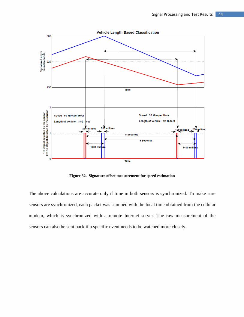
Figure 32 shows that the distance between the two sensors is traversed in approximately five

seconds for two sample vehicles. This results in an estimated speed of 50 mph for each vehicle.

(The time offset can also be used for estimating the vehicle length. In this example while both

vehicles have similar speed, the length of the first vehicle is approximately 12 - 15ft. and the

second vehicle is approximately 18 - 21ft. Length-based calculations will be discussed more

fully in section 5.4.)


Figure 32. Signature offset measurement for speed estimation

The above calculations are accurate only if time in both sensors is synchronized. To make sure

sensors are synchronized, each packet was stamped with the local time obtained from the cellular

modem, which is synchronized with a remote Internet server. The raw measurement of the

sensors can also be sent back if a specific event needs to be watched more closely.


5.4. Length-based Classification

After receiving the packets from the installed sensors, the data collector puts a time stamp on

each packet. Because the coordinator’s internal time is continuously updated through the modem

connection, a synchronized array of events (e.g., detection of vehicles, or keep-alive signal) are

always obtained from two consecutive sensors. Additionally, there is a low chance that one car

can overtake the other in the short distance between two sensors, considering typical highway

speeds on the highway.

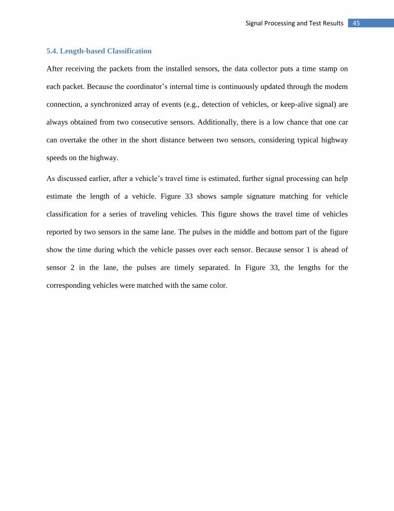
As discussed earlier, after a vehicle’s travel time is estimated, further signal processing can help

estimate the length of a vehicle. Figure 33 shows sample signature matching for vehicle

classification for a series of traveling vehicles. This figure shows the travel time of vehicles

reported by two sensors in the same lane. The pulses in the middle and bottom part of the figure

show the time during which the vehicle passes over each sensor. Because sensor 1 is ahead of

sensor 2 in the lane, the pulses are timely separated. In Figure 33, the lengths for the

corresponding vehicles were matched with the same color.


Figure 33. Signature matching for length based classification

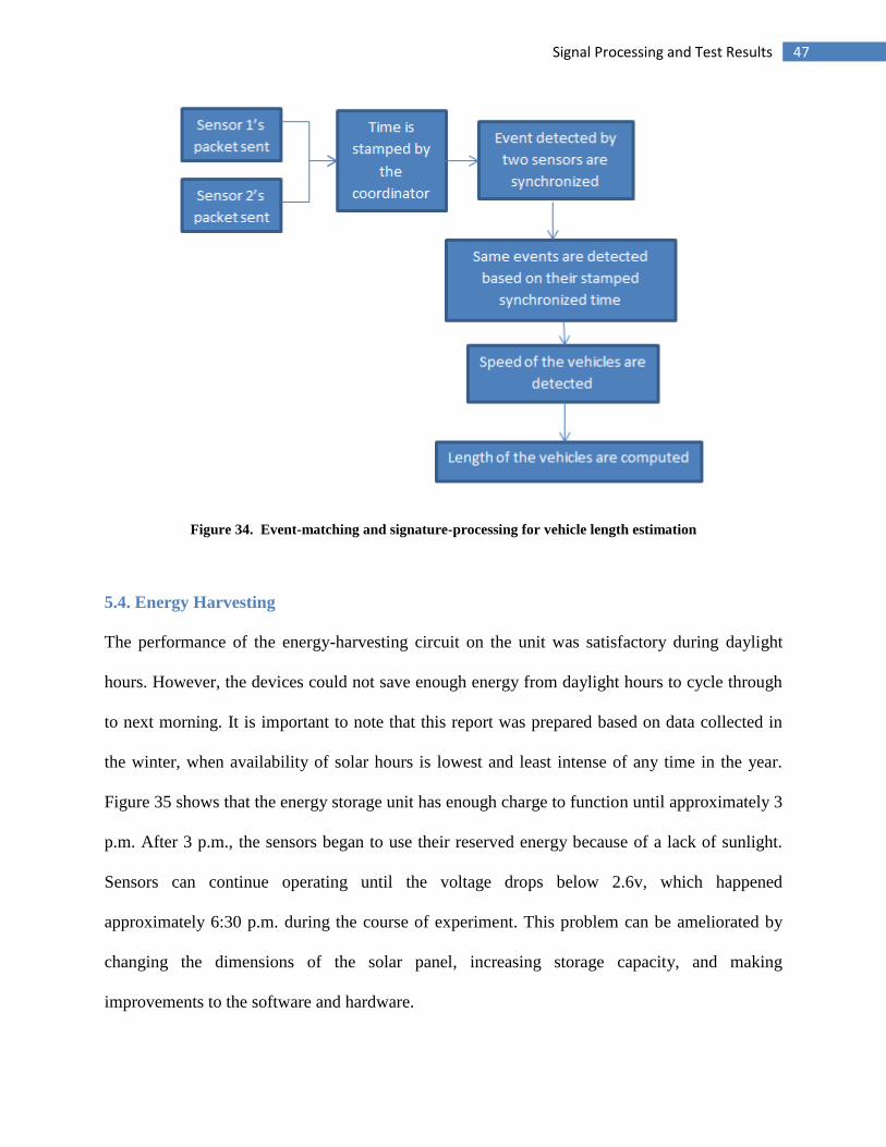
The classification algorithm is summarized in the flow chart shown in Figure 34.


Figure 34. Event-matching and signature-processing for vehicle length estimation

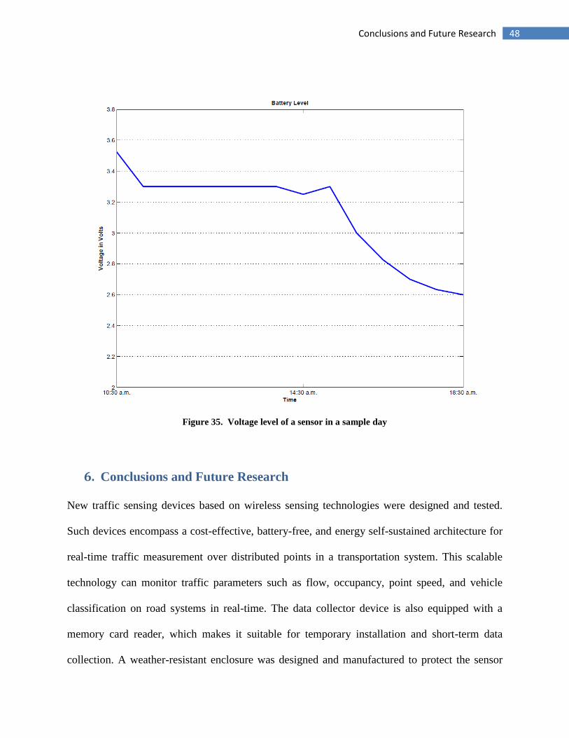
5.4. Energy Harvesting

The performance of the energy-harvesting circuit on the unit was satisfactory during daylight

hours. However, the devices could not save enough energy from daylight hours to cycle through

to next morning. It is important to note that this report was prepared based on data collected in

the winter, when availability of solar hours is lowest and least intense of any time in the year.

Figure 35 shows that the energy storage unit has enough charge to function until approximately 3

p.m. After 3 p.m., the sensors began to use their reserved energy because of a lack of sunlight.

Sensors can continue operating until the voltage drops below 2.6v, which happened

approximately 6:30 p.m. during the course of experiment. This problem can be ameliorated by

changing the dimensions of the solar panel, increasing storage capacity, and making

improvements to the software and hardware.

48 Conclusions and Future Research

Figure 35. Voltage level of a sensor in a sample day

6. Conclusions and Future Research

New traffic sensing devices based on wireless sensing technologies were designed and tested.

Such devices encompass a cost-effective, battery-free, and energy self-sustained architecture for

real-time traffic measurement over distributed points in a transportation system. This scalable

technology can monitor traffic parameters such as flow, occupancy, point speed, and vehicle

classification on road systems in real-time. The data collector device is also equipped with a

memory card reader, which makes it suitable for temporary installation and short-term data

collection. A weather-resistant enclosure was designed and manufactured to protect the sensor


from vehicle impacts on the highway. In addition to traditional traffic parameters, the sensors can

measure and report the temperature of their surroundings because they are surface-mounted. The

sensors developed as a result of this project are also capable of capturing a digital magnetic

signature of vehicles within any intervals required by clients. The digital magnetic signature was

processed to calculate traffic volume, vehicle speed, and vehicle length estimation for

classification. With the help from SHA and Inter County Connector staff, five sensors were

permanently deployed and thoroughly tested on a section of the ICC. Lane-by-lane data on this

segment of the highway is reported and archived in a server on the UM campus. The results

indicate that the developed wireless vehicle sensing architecture can be adapted for a range of

traffic management applications. Direction for future research includes:

The sensors developed as a result of this project are capable of collecting high-resolution

magnetic signatures, which, after signal processing, can be used for anonymous vehicle

matching and tracking. The experiments conducted during the course of this project show

the reliability of the magnetic signatures data collection and the potential for travel time

and OD estimation. However, given energy limitations, further research is needed to

develop ultra-efficient signal processing algorithms for signature-matching purposes.

Transmitting a high-resolution signature is energy intensive. To overcome the energy

constraint, the devices built for this project took advantage of a modified and condensed

version of the digital signature to re-identify vehicles based on their length and to provide

length-based classification. However, with further research and modifications in

hardware and software, obtaining and communicating higher resolution signals will be

possible. In the final month of the project schedule, a new ultra-low-power AMR sensing

element was introduced to the market. This new AMR sensing element provides a greater


sampling rate and requires much less energy compared to current elements available in

the commercial market. The flexibility of the hardware design in this project will allow

adoption of such technologies. Further research is needed to implement efficient and

advanced signal processing algorithms in the microcontroller so that important features of

the signal can be extracted to reduce the signature into information before transmitting to

the data collector.

In this project, the sensors were surface-mounted. However, in special infrastructures

(such as tunnels where only two lanes exist), these sensors can be modified to be wall-

mounted. This adaptability will make the installation of sensors easy and will also allow

for data collection on these critical facilities with high granularity. Additionally, the

energy harvesting component of these sensors can be eliminated and replaced with a

battery pack to increase reliability of the data collection system and to address the lack of

ambient light in tunnels. The operators will still be able to monitor traffic volume, speed,

headway, and occupancy for each lane. Mounting sensors on tunnel walls will allow for

the accurate measurement of the queue length if incidents happen and traffic backs up in

the tunnel.

New technologies for travel-time measurement (such as Bluetooth sensors) collect a

sample from the traffic stream and estimate the travel time for a particular segment.

Although the data provided by such technologies (such as travel time and average speed)

provided by such technologies is useful, having traffic volume data on the corresponding

segments is needed to understand the dynamics of the underlying traffic conditions. The

sensors developed in this project can be modified to synchronize with Bluetooth detectors

and provide an accurate picture of the dynamics of underlying traffic conditions. By


developing sensors that combine Bluetooth and wireless magnetic technologies, the

penetration rate of Bluetooth can be measured. The system can also be used for analyzing

vehicular movements and traffic patterns at locations where highways merge or split.

Applications include dynamic message sign (DMS) operation analysis and highway OD

estimation. An additional limitation of Bluetooth detectors and probe-based data such as

INRIX travel time is that they are incapable of separating data by lane, which necessitates

additional devices for collecting data to monitor traffic conditions. However, the wireless

magnetic sensors developed for this project can supplement these Bluetooth detectors and

probe-based technologies.

The sensors created for this project were developed to collect data about highway traffic

in which vehicles travel at relatively high speeds. However, the sensors can be modified

and calibrated for arterial operations. By deploying multiple sensors at intersections, the

presence of vehicles and the length of the queue behind the stop bar can be measured and

communicated to the signal controller.

52 References

7. References

1. Traffic Congestion and Reliability, FHWA, September 2005

2. Texas Transportation Institute, Urban Mobility Report, 2005.

3. A. Kansal, D. Potter, and M. Srivastava. Performance aware tasking for environmentally

powered sensor networks. In ACM Joint International Conference on Measurement and

Modeling of Computer Systems (SIGMETRICS).

4. Honeywell International Inc., “Application Note Vehicle Detection Using AMR

Sensors,” available at http://www.magneticsensors.com/datasheets/an218.pdf

5. M. Kalantari and M. Shayman. Design optimization of multi-sink sensor networks by

analogy to electrostatic theory. In IEEE Wireless Communications and Networking

Conference, April 2006.

6. M. Kalantari and M. Shayman. Energy efficient routing in wireless sensor networks.

Conference on Information Sciences and Systems, Princeton University, March 2004.

Traffic Data Collection and Anonymous Vehicle … DATA COLLECTION AND ANONYMOUS VEHICLE ... TRAFFIC...

Documents

Transcript of Traffic Data Collection and Anonymous Vehicle … DATA COLLECTION AND ANONYMOUS VEHICLE ... TRAFFIC...