Traffic Characteristics for Implementation and Calibration of Freeway Merging Control Systems JOHANN H. BUHR, ROBERT H. WHITSON, KENNETH A. BREWER, and DONALD R. DREW, Texas Transportation Institute, Texas A&M University

Using the Gulf Freeway in Houston as the laboratory, a number of traffic characteristics associated with gap acceptance con­trol were studied. Data collection was performed using manual methods, a closed-circuit television system, and an electronic data acquisition system including field sensors and a digital computer.

The ramp traffic characteristics presented include the ve -hicle performance characteristics of speed, acceleration, and travel time, the relationships among these variables, and the effects of vehicle type and ramp grade on these variables. The behavior of ramp vehicles at the control signal was also studied to determine the starting-delay characteristics and stopping position of vehicles at the ramp signal. A frequency distribu­tion of each variable is presented and the application of the results in the implementation and calibration of merging con -trol systems is discussed.

Several freeway traffic characteristics were also studied These were concerned mainly with traffic stability upstream from an entrance ramp and the effect of this stability on the accuracy with which the trajectory of a ramp vehicle can be matched with afreeway gap. Also presentedis the relationship between total travel and total travel time, two measures of ef­fectiveness often used in the evaluation of freeway control sys -terns. The possible application of this relationship in the de -velopment of warrants for freeway control is indicated.

•IN March of 1966, the first prototype automatic traffic-responsive merging controller was installed on the Telephone Road inbound entrance ramp of the Gulf Freeway in Houston. Since that time, considerable experience has been gained with the operation of this type of instrument and its effect on traffic behavior. This has led to the de­velopment of first-generation and second-generation controllers of an increasingly complex nature. The rapidity of these developments has caused the accompanying expansion of knowledge to be limited to relatively few researchers and practicing traf­fic engineers. Much of the new technology is of a rather subjective nature, based on the day-to-day observation of the operation of these controllers over a long period of time. Documentation of findings, both speculative and factual, has lagged far behind. Many of the more subjective aspects of the controlled operation are difficult or im -possible to measure or otherwise pin down factually, so that researchers are under­stanc;lably loath to record their views on these matters. However, there are a number of readily measurable traffic characteristics that affect the design and operation of a control system and that are affected by the control system. The objective of this paper is to document these characteristics. It is an outgrowth of a research project

Paper sponsored by Committee on Characteristics of Traffic Flow and presented at the 48th Annual Meeting.

87

88

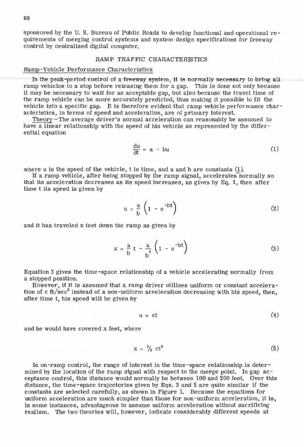
sponsored by the U. S. Bureau of Public Roads to develop functional and operational re­quirements of merging control systems and system design specifications for freeway control by centralized digital computer.

RAMP TRAFF1C CHARACTERISTICS

Ramp-Vehicle Performance Characteristics

In the peak-period control of a freeway system, it is normally necessary to bring all ramp vehicles to a stop before releasing them for a gap. This is done not only because it may be necessary to wait for an acceptable gap, but also because the travel time of the ramp vehicle can be more accurately predicted, thus making it possible to fit the vehicle into a specific gap. It is therefore evident that ramp vehicle performance char­acteristics, in terms of speed and acceleration, are of primary interest.

Theory-The average driver's normal acceleration can reasonably be assumed to have a linear relationship with the speed of his vehicle as represented by the differ­ential equation

du dt=a-bu (1)

where u is the speed of the vehicle, t is time, and a and b are constants (1). If a ramp vehicle, after being stopped by the ramp signal, accelerates -normally so

that its acceleration decreases as its speed increases, as given by Eq. 1, then after time t its speed is given by

a ( -bt) U=b 1-e (2)

and it has traveled x feet down the ramp as given by

(3)

Equation 3 gives the time-space relationship of a vehicle accelerating normally from a stopped position.

However, if it is assumed that a ramp driver utilizes uniform or constant accelera -tion of c ft/sec 2 instead of a non-uniform acceleration decreas ing with his speed, then, after time t, his speed will be given by

u = ct (4)

and he would have covered x feet, where

x = % ct2 (5)

In on-ramp control, the range of interest in the time -space relationship is deter­mined by the location of the ramp signal with respect to the merge point. In gap ac­ceptance control, this distance would normally be between 100 and 200 feet. Over this distance, the time-space trajectories given by Eqs. 3 and 5 are quite similar if the constants are selected carefully, as shown in Figure 1. Because the equations for uniform acceleration are much simpler than those for non-uniform acceleration, it is, in some instances, advantageous to assume uniform acceleration without sacrificing realism. The two theories will, however, indicate considerably different speeds at

89

180 10

160 8

0 ... ~

I- :c 6 ... 140 Q. ...

~ u.

~ z ... 0 <J ~ z .. 120 a: 4 I- w (/) _J

c w <J <J ..

100 2

I -- UNIFORM ACCELERATION

I -----NON-UNIFORM ACCELERATICN

80 10 20 30 4 15 6 7 B 9 40 50

TIME IN SECONDS SPEED (MPH)

Figure l. Comparison of time-space traces given by uniform and non-uniform acceleration.

Figure 2. Acee leration vs speed of passenger ve­hicle during normal acceleration from a standing

start on an entrance ramp.

various points on the ramp. The researcher should, therefore, be mindful of the effects of substituting one theory for another.

Study Procedure-In order to evaluate the constants that define the speed-accelera -tion characteristics of ramp vehicles, several runs were made- on both controlled and uncontrolled ramps using a 1966 Plymouth Station Wagon equipped with a V8 engine and automatic transmission and instrumented with a recording speedometer. Several driv­ers were used and only smooth merges were included in the analysis. On the few un -controlled ramps studied, the vehicle was brought to a stop on the ramp before accel -erating on to the merge area. From the recorded time-speed trace, the acceleration was calculated over every 2-mph increase in speed The accelerations were then plot­ted against the speeds, and straight lines fitted through the points.

Results-The results of these experiments showed quite similar speed-acceleration characteristics for different drivers and different ramps, except for some isolated runs. Figure 2 shows the results of four runs made by the same driver on the Telephone in­bound entrance ramp (zero grade) on the Gulf Freeway (correlation coefficient= 0.85 with Eq. 1). It is representative of all the runs recorded. The values of the parameters a and b-1 yielded by these experiments are approximately 10 mph/sec (15 ft/sec 2

) and 4 seconds, respectively.

These results are quite different from those found by other experimenters whose studies, performed under differe.nt conditions, yielded values of a ranging between 4 and 7 mph/sec with b-1 ranging between 20 and 15 seconds (2, 3 ). These differences are illustrated in Figure 3. - -

The Effect of Grades -To evaluate the effect of grades on the speed-acceleration char­acteristics of passenger vehicles on an entrance ramp, studies as described above were also performed on th.e Griggs inbound entrance ramp on the Gulf Freeway (3 percent upgrade) and on the Newcastle inbound entrance ramp (5 percent upgrade) on the Southwest Free­way in Houston. The results of four test runs on Griggs and three test runs on New­castle are shown in Figures 4 and 5, respectively, with correlation coefficients of 0. 84 and 0.87. From the figures it would appear that on the steeper ramp the vehicle gen­erally utilized a slightly greater acceleration than on the less steep ramp. To compare these characteristics with those of a level ramp, the results obtained on the Telephone (zero grade), the Griggs (3 percent upgrade), and the Newcastle (5 percent upgrade) ramps are superimposed in Figure 6. These results indicate that vehicles apparently utilize greater acceleration on steeper ramps.

90

z 0

10

8

li a: 4 UJ _, UJ

~ 2

MATSON, SMITH

TRANSPORTATION INSTITUTE ( 1968)

TRAFFIC ENGINEERING HANDBOOK (1958- 591

AND HURD ( 1952)

o~~~~~~--'~~~-'-~~~~~--'

0 10 20 30 40

SPEED (MPHI

Figure 3. Comparison of speed-acceleration characteristics found by different

experimenters.

50

10

8

0 UJ

!'.' :c + + Q. 6 ~

z 0

>= <I 4 a: UJ _, + UJ 0

~

2 +

0 0 10 20 30 40 50

SPEED (MPH)

Figure 4. Speed-acceleration characteristics on the Griggs Road entrance ramp (3 percent upgrade).

Ramp Travel Times, Speeds , and Accelerations

The travel time of a ramp vehicle on a controlled ramp is considered here to be that time which expires between the instant the ramp signal turns green and the instant the vehicle actuates a merge detector located at the physical nose of the ramp. This im -portant variable affects the controller settings and places certain limitations on the de­tector layout of a control system, and its variation affe cts the number of vehicles that will actually "hit" their assigned gaps (4).

Data Collection -The data required to study the travel -time characteristics of ve -hicles on a controlled ramp were measured and recorded by the digital computer being used to control the ramps. The data were collected only for those merging vehicles

that had a clear and unoccupied ramp ahead as they were released at the ramp

10 signal. Travel times were sampled on + + + + each of six ramps during two morning

8

+ u UJ

'2 :c Q. 6 !

+ z 0 >= .. 4 a: UJ _, UJ 0 0 ..

2

0 0 10 20 30 40 50

SPEED (MPH)

Figure 5. Speed-acceleration characteristics on the Newcastle entrance ramp (5 percent upgrade).

peak hours .

12 u UJ V> .... :c Q.

! a z 0

!i a: UJ _J 4 UJ 0 (.) <I

0 0 10 20 30 40

SPEED(MPHI

Figure 6. Effect of ramp grade on speed­acceleration characteristic of passenger car.

50

91

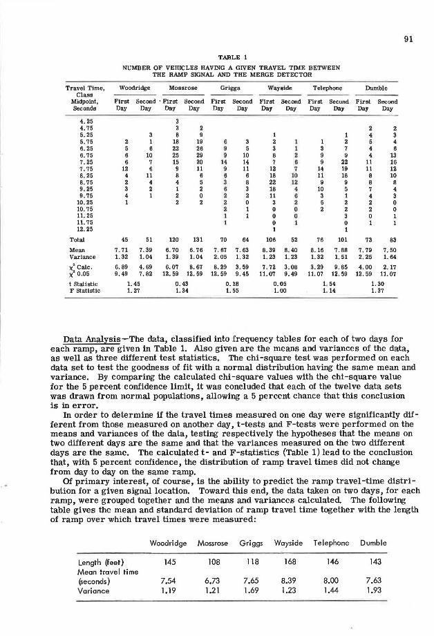
TABLE 1

NUMBER OF VEHICLES HAVING A GIVEN TRAVEL TIME BETWEEN THE RAMP SIGNAL AND THE MERGE DETECTOR

Travel Time, Woodridge Mossrose Griggs Wayside Telephone Dumble Class

Midpoint, First Second · First Second First Second F irst Second First Second F irst Second Seconds Day Day Day Day Day Day Day Day Day Day Day Day

4. 25 3 4. 75 3 2 2 2 5. 25 3 8 9 1 1 4 3 5. 75 2 1 18 19 6 3 2 l 1 2 5 4 6. 25 5 6 22 26 9 5 3 1 3 7 4 6 6. 75 6 10 25 29 9 10 8 2 9 9 4 13 7.25 6 7 15 20 14 14 7 6 9 22 11 16 7 . 75 12 6 9 11 9 11 12 7 14 19 11 12 8.25 4 11 8 6 6 6 18 10 11 18 8 10 8. 75 2 4 4 5 3 8 22 12 9 9 8 8 9. 25 3 2 1 2 6 3 18 4 10 5 7 4 9.75 4 1 2 0 2 2 11 6 3 1 4 3

10. 25 1 2 2 2 0 3 2 5 2 2 0 10. 75 2 1 0 0 2 2 2 0 11 . 25 1 1 0 0 3 0 1 11 . 75 1 0 l 0 1 1 12.25 1 1

Total 45 51 120 131 70 64 106 52 76 101 73 83

Mean 7. 71 7. 39 6. 70 6. 76 7. 67 7 . 63 8. 39 8. 40 8. 16 7. 88 7. 79 7. 50 Variance 1. 32 1. 04 1. 39 1. 04 2.05 1. 32 1. 23 1. 23 1. 32 1. 51 2. 25 1. 64

x2 Cale. 6. 89 4. 69 6.07 8. 67 8.29 3. 59 7.72 3.08 3. 29 9.85 4.00 2.17 x2 o .o5 9. 49 7. 82 12. 59 12.59 12. 59 9.45 11. 07 9.49 11 . 07 12. 59 12 . 59 11.07

t statistic 1.45 0.43 0.18 0.05 1. 54 1. 30 F statistic 1. 27 1. 34 1. 55 1. 00 1. 14 1. 37

Data Analysis-The data, classified into frequency tables for each of two days for each ramp, are given in Table 1. Also given are the means and variances of the data, as well as three different test statistics. The chi-square test was performed on each data set to test the goodness of fit with a normal distribution having the same mean and variance. By comparing the calculated chi -square values with the chi-square value for the 5 percent confidence limit, it was concluded that each of the twelve data sets was drawn from normal populations, allowing a 5 percent chance that this conclusion is in error.

In order to determine if the travel times measured on one day were significantly dif­ferent from those measured on another day, t-tests and F-tests were performed on the means and variances of the data, testing respectively the hypotheses that the means on two different days are the same and that the variances measured on the two different days are the same. The calculated t- and F-statistics (Table 1) lead to the conclusion that, with 5 percent confidence, the distribution of ramp travel times did not change from day to day on the same ramp.

Of primary interest, of course, is the ability to predict the ramp travel -time distri -bution for a given signal location. Toward this end, the data taken on two days, for each ramp, were grouped together and the means and variances calculated The following table gives the mean and standard deviation of ramp travel time together with the length of ramp over which travel times were measured:

Woodridge Moss rose Griggs Wayside Telephone Dumb le

Length (feet) 145 108 118 168 146 143 Mean travel time ~econds) 7.54 6.73 7.65 8.39 8.00 7.63 Variance l .19 l.21 l .69 1.23 l.44 1.93

92

These travel times include the starting delays of drivers at the signal. By plotting these data points on time and distance coordinates and superimposing the plot over time -space graphs, the starting delay and the acceleration rates can be estimated. By assuming non-uniform acceleration and using the parameter of a= 10 mph/sec and b-1 = 4 se onds derived earlier, the starting delay was estimated to be 2. 4 seconds. For the sake of simplicity a uniform acceleration of 10 ft/sec, together with a starting delay of 2.4 seconds, can be used. For all practical purposes, over the range of ramp lengths of from 80 to 200 feet, the ramp travel time of the average vehicle on a level ramp can be consider ed as being given by

Travel time = 2.4 + f dis~~~ce The variances measured at the six different ramps as given in the table indicate

that, over the distances covered (110 feet to 170 feet), there is apparently no relation­ship between the distance traveled and the variance in travel time.

Conclusions-The following conclusions are warranted:

1. For purposes of predicting the ramp travel time on a controlled ramp, it makes practically no difference whether uniform or non-uniform acceleration is assumed over the normal range of ramp signal locations.

2. If uniform acceleration is assumed, then it is reasonable to assume that the aver­age vehicle has a starting delay of 2.4 seconds and an acceleration of 10.0 ft/sec 2

; if non-uniform acceleration is assumed, then it is reasonable to assume that the average vehicle has a starting delay of 2.4 seconds and a maxim um acceleration of 10 mph/sec, which decreases linearly by 7'4 mph/sec for every 1-mph increase in vehicle speed.

3. Ramp travel times, on a controlled ramp where all vehicles are brought to a stop before they are released for a gap, are uniformly distributed, with the mean related to the distance traveled as mentioned in conclusion 2.

4. The distribution of ramp travel times on the same ramp does not change from day to day.

5. The ramp travel times were not markedly more variable over the longer ramps than over the shorter ramps studied.

The Value of Hitting a Gap

The foregoing data pertained to vehicles whose progress up the ramp was unimpeded and, therefore, were able to enter the freeway smoothly, performing ideal merges. The provision of ideal merging opportunities is one of the two objectives of merging control systems (5). In many cases, when a ramp driver misses his assigned gap he is forced to stop on the acceleration lane and wait for an acceptable gap. Since the relative speed is now greatly increased, the size of the acceptable gap is also increased, necessitating a longer wait for the stopped driver as well as for other drivers desiring to enter the ramp (6 ). This increased delay reduces the service volume of an entrance ramp, as illustrated by the capacity curves developed by Brewer et al (7 ). The value of fitting a vehicle into a gap under such conditions is evident. -

When the freeway volume is fairly low, chances are that a ramp vehicle missing its assigned gap may find another gap to enter into without having to come to a complete stop. Even under these conditions, however , missing the assigned gap has a detrimen­tal effect on ramp operation. This is illustrated by Figure 7, which shows the time­speed traces recorded by an instrumented vehicle under three conditions when it hit its assigned gap and under three conditions when it did not. The detrimental effect of not hitting its assigned gap is immediately evident.

As a quantitative measure of this effect, the acceleration noise experienced by the driver was calculated for eight runs in which the driver performed an ideal merge and five runs in which he missed the gap but still entered the freeway without having to stop.

" .. !

x

93

TIME

TIME

Figure 7. Recording speedometer traces of ramp vehicle: (top) matched with acceptable gap; (bottom) not matched with acceptable gap.

The average acceleration noise for the eight ideal merges was 2.23 mph/sec, and for the five merges in which the driver missed his assigned gap, it was 3. 91 mph/sec.

Number of Vehicles Hitting Gaps-In order to study the effect of gap-acceptance con­trol on merging behavior, studies were carried out on five entrance ramps during the periods of afternoon control by digital computer. During the afternoon, it is considered that freeway capacity is not a problem. The first objective of a merging control sys­tem, that of prevention of congestion, is therefore not a factor in afternoon control. How­ever, ramp volumes are generally higher during the afternoon peak than during the morning peak. These studies therefore isolate the second objective, that of improving merging conditions.

In these studies, observers classified all ramp vehicles first into two groups -those that used the ramp signal correctly (called non-violators) and those that "ran" the red signal (called violators). The non-violators were then further classified into one of four groups-those that ''hit'' gaps (assumed to be their assigned gaps) and were thus able to perform smooth ideal merges; those that were matched with their assigned gaps but refused them and accepted another gap without first stopping; those that missed their assigned gaps and entered another gap without stopping; and finally, those that stopped on the ramp or acceleration lane before merging either because no gap was available or because another vehicle was stopped in the merging area. Violators were classified into one of three groups-those that met gaps and performed smooth merges; those that did not immediately meet a gap but were still able to merge without stopping; and those that stopped before merging. Studies were made for a period of 1 hour dur­ing the afternoon control, which lasts 1 % hours . Data were collected for each 5-minute period during the study. Altogether, 31 studies were made, covering 370 five-minute periods. Observations were taken on 9831 ramp vehicles.

In order to investigate whether the percentage of vehicles in each group was affected by the freeway volume, plots were drawn up of the percentage in each group, based on 15-minute totals, against the freeway outside lane volume, based on 15-minute counts

94

"' 100

w _J

" 90 i: w > a. Vi :IE IC .. 0 IC I- 70 .. _J _J

_J 0 MEAN .. > .. z 0 0 • o

I- ~ z w

" IC w a. 30

100

• WOODRIDGE

• GRIGGS

o WAYSIDE

a. iEL Ef'HONE

X DU MSLE ~ . . - • • . ~ . . ' ~· .

' . ' .. 0 ·. . .

•, . r

. .t ~ ~ • 800 <JOO IOOO 1100 1200 1300 14 00 1500

FREEWAY OUTSIDE LANE VOLUME UPSTREAM OF MERGING AREA

(VPH BASED ON 15 MINUTE FLOW RATE)

. . ~

.. 1600

Figure 8. Relationship between freeway volume and frequency of srnool'f1 merges for gap-acceptance control by digital computer.

by the digital computer. (Freeway counts were not available for some of the study days.) Figure 8 shows the plot of non-violators performing smooth merges as a per­centage of all ramp vehicles, against the freeway outside lane flow rate. This plot is typical of all the other groups (except for the magnitude of the percentage). No trend is evident, and the conclusion is, therefore, that the percentage of ramp vehicles in each of the aforementioned groups is not affected by the freeway volume. Because of this conclusion, all the data for each ramp were grouped together. The results are shown in Figure 9. Since the percentages of vehicles that missed or refused gaps but still entered without s topping were r elative ly s mall, both violators and non-violators are shown in two groups only-those that merged smoothly and those that did not meet a gap. The full distinction is made in the column representing the results of all data grouped together.

The vehicles in each group, as a percentage of non-violators and of violators, are shown in Figure 10. Violators, being generally the more aggressive drivers, did not perform much worse than non-violators. However, both groups performed much better than on uncontrolled ramps. The uncontrolled data are based on five studies performed on two of the ramps before control was initiated.

In interpreting the results, it should be borne in mind that these are the results of actual studies and that they do not represent the best performance that can be expected

"' "' ...J 0 ;:

IC>C)o

"' 10 > 0

"' > II: tn 10 ID 0

...J

...J .. .. ~

~ .. ~ 20 w 1f "' 0..

"' ~ a ;;;

~ l:i ..

] ~~

w d ~

~~ ~ 2

~ ~ 8 T Q~C(

~~~ g2 ..J/L

REFUSED GAP

Figure 9. Results of gap-acceptance studies during afternoon control.

100

80

UJ 60 to <( f-z UJ u a::

"' 40 IL

20

NON -VIOLATORS

ENTERED GAP SMOOTHLY

STOPPED IN MERGING AREA

VIOLATORS UNCONTROLLED RAMPS

95

Figure 10. Merging characteristics of non-violators and violators compared with an uncontrolled ramp.

of gap-acceptance control. For example, many vehicles stopped in the merging area actually would have hit their gaps but were forced to stop because the preceding vehicle stopped in the merging area. This happens because the merge detector is located so far from the ramp signal that invariably a second vehicle will be released before the merge override is called in (4). This situation should be practically eliminated by the newer, second-generation controllers. The non-violators hitting gaps plus those re­fusing gaps give a better indication of the capability of the controllers to match ramp vehicles with gaps. However, a number of vehicles that were actually matched with gaps and refused these gaps were forced to stop before merging. These are therefore included in the latter group. Furthermore, the percentage of drivers violating the ramp signal is quite large on all ramps. With some degree of enforcement, the situation could be substantially improved.

Signal Violations-The foregoing data show a high proportion of violators onallramps. Signal violations have been a problem in the afternoon control from the start. In six months of control on a day-to-day basis, the percentage of violations has decreased only slightly. For one week, policemen were stationed in the vicinity of the ramp signals. During this week, violations decreased to practically nothing, but returned to the orig­inal percentage after the policemen left. During the morning control, when high densi­ties on the freeway make the need for the ramp control much more evident, the propor­tion of violations is much lower. The following table, based on observations taken during five to eight control periods on each ramp, gives the average percentage of ramp signal violations:

Woodridge Wayside Telephone Griggs Dumble

Afternoon control Morning control

19.6 5.4

Ramp Travel Times by Vehicle Types

14.9 7.7

18.1 5.4

13.9 8.3

15.l 6.0

Where loaded trucks and other heavy or slow vehicles form a substantial part of the ramp traffic, it may be important to design the ramp control system so as to give special consideration to these types of vehicles. Such special consideration may, for example, take the form of allowing for a longer ramp travel time, releasing the vehicle for a

96

bigger gap, and holding the signal in red until the vehicle has cleared the merging area. This may eventually involve the automatic recognition of vehicles with different weight/ horsepower ratios. In order to develop special considerations for these vehicles, their relative operating characteristics must be known. One characteristic needed is the ramp travel time from a stopped position at the ramp signal.

Sludy Procedure - About 100 ramp travel times were measured for each of four dif­ferent types of vehicles. Because the truck traffic on any of the Gulf Freeway ramps is very light, the data from Woodridge, Dumble, Wayside, and Telephone ramps were grouped together. In each case, the travel time was measured from the instant that the ramp signal turned green until the instant that the vehicle reached a point about 200 feet downstream from the signal. This point is further down the ramp than the merge de­tector to which the travel times analyzed earlier were measured. It is located approx­imately at the painted nose of the ramp, whereas the merge detectors are usually lo­cated at the physical nose of the ramp.

Results-The data collected were grouped, by class, into frequency tables and their means and variances calculated as given in Table 2. Also shown are the calculated and theoretical chi-square values obtained by fitting the data to normal distributions. The chi-square tests indicate that the travel times for each class of vehicle can sta­tistically be considered as being normally distributed. The results of t- and F-tests in Table 2 lead to the conclusion that different classes of vehicles have significantly different mean travel times and that the variation within one class does not differ sig­nificantly from the variation within the adjacent class.

Conclusions-With regard to different vehicle types, it can be concluded that:

1. The ramp travel times of different classes of vehicles are normally distributed within each class;

2. The average ramp travel time of a certain class of vehicles is significantly shorter than the average travel time of any class of larger vehicles; and

TABLE 2

RAMP TRAVEL TIMES FOR DIFFERENT CLASSES OF VEHICLES

Travel Time, Frequency of Occurrence Class

Midpoint, Compact Passenger Single-Unit Tractor-Seconds Cars Cars Trucks Trailers

5. 75 3 6.25 1 1 6. 75 1 3 7.25 14 9 3 7.75 8 8 4 8.25 21 16 5 8.75 13 10 6 9.25 17 14 14 2 9.75 7 9 11 4

10. 25 7 11 13 10 10.75 1 6 8 3 11. 25 1 5 12 12 11. 75 3 3 6 12.25 6 13 12. 75 1 9 13. 25 3 5 13. 75 7 14.25 10 14. 75 4 15.25 4 15.75 1 16.25 1

Total 94 95 89 91

Mean 8.42 8.98 9.99 12. 37 Variance 1. 17 1. 77 1. 96 2. 86

x' Cale . 10. 30 7.40 7. 75 9.11 x' o.o5 11.07 14.07 14.07 14.07

t Statistic 3.18 5.02 10.29 F Statistic 1. 51 1. 11 1. 46

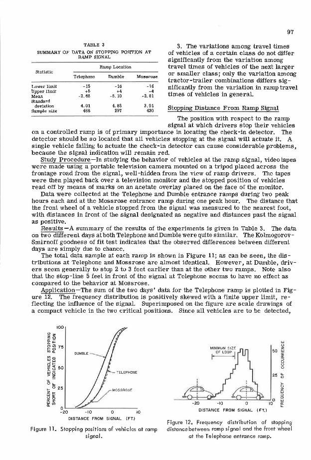
TABLE 3

SUMMARY OF DATA ON STOPPING POSITION AT RAMP SIGNAL

Ramp Location Statistic

Telephone Dumble Mossrose

Lower limit -15 -16 -16 Upper limit +5 +4 +4 Mean -2.68 -5. 10 -2.81 Standard

deviation 4.01 4. 83 3.91 Sample size 488 297 430

97

3. The variations among travel times of vehicles of a certain class do not differ significantly from the variation among travel times of vehicles of the next larger or smaller class; only the variation among tractor-trailer combinations differs sig­nificantly from the variation in ramp travel times of vehicles in general.

Stopping Distance From Ramp Signal

The position with respect to the ramp signal at which drivers stop their vehicles

on a controlled ramp is of primary importance in locating the check-in detector. The detector should be so located that all veh~cles stopping at the signal will actuate it. A single vehicle failing to actuate the check-in detector can cause considerable problems, because the signal indication will remain red.

Study Procedure-In studying the behavior of vehicles at the ramp signal, videotapes were made using a portable television camera mounted on a tripod placed across the frontage road from the signal, well-hidden from the view of ramp drivers. The tapes were then played back over a television monitor and the stopped position of vehicles read off by means of marks on an acetate overlay placed on the face of the monitor.

Data were collected at the Telephone and Dumble entrance ramps during two peak hours each and at the Mossrose entrance ramp during one peak hour. The distance that the front wheel of a vehicle stopped from the signal was measured to the nearest foot, with distances in front of the signal designated as negative and distances past the signal as positive.

Results-A summary of the results of the experiments is given in Table 3. The data on two different days at both Telephone andDumble were quite similar. The Kolmogorov­Smirnoff goodness of fit test indicates that the observed differences between different days are simply due to chance.

The total data sample at each ramp is shown in Figure 11; as can be seen, the dis­tributions at Telephone and Moss rose are almost identical. However, at Dumble, driv­ers seem generally to stop 2 to 3 feet earlier than at the other two ramps. Note also that the stop-line 5 feet in front of the signal at Telephone seems to have no effect as compared to the behavior at Mossrose.

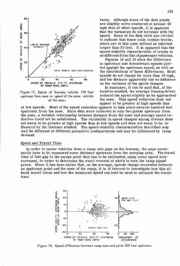
Application-The sum of the two days' data for the Telephone ramp is plotted in Fig­ure 12. The frequency distribution is positively skewed with a finite upper limit, re­flecting the influence of the signal. Superimposed on the figure are scale drawings of a compact vehicle in the two critical positions. Since all vehicles are to be detected,

"'z ~o

100

~~ ~ ~ 75 (/) Q.

(/) c "'w d I-;: ~ 50 w->~ u. 0 u. I- 0 25 z 1-w a: '-' 0

~ V5 Q L-_.:;...o:..~~~~~~~-

-20 -10 0 10

DISTANCE FROM SIGNAL (FT.)

Figure 11. Stopping positions of vehicles at ramp signal.

w '-' z

50 w a: a: ;;;;)

'-' '-' 0

25 u. 0

,.. '-' z w ;;;;)

0 0 w

-20 -10 0 10 a: u.

DISTANCE FROM SIGNAL (FT.)

Figure 12. Frequency distribution of stopping distance between ramp signal and the front wheel

at the Telephone entrance ramp.

98

I I-(!) z LI.I ...J

fil 100 ~ -- GAP-ACCEPTANCE CONTROL

LI.I u :::i i3 -- - NO CONTROL LI.I ~

ea :::i 0 c /NUMBER OF STUDIES (HRS.)

~ LI.I c

60 I LI.I ' I- LI.I

"~ " u LI.I x ~ LI.I ' j:: a:: ~a ' 0 ' IL ' 0 0 ' .... I- LI.I

20 - ..... ' z ...J

LI.I ...J

~ <[ :::i

~ 0 LI.I

0 2 4 6 8 10 12 14

QUEUE LENGTH (VEHS.)

Figure 13. Number of vehicles between back of queue and merge point.

the location and size of the check-in loop should be based on the smallest vehicle stopped at the two extremes of the frequency distribution. By allowing a 1-foot overhang into the loop in either position, it is clear that, based on the Telephone data, the min­imum length of the loop should be 9 feet and the loop should be located no further than 5 feet from the signal. Based on the Dumble data, the loop should be of the same length, but the trailing edge would be 6 feet from the signal. When all three ramps studied are considered together, a loop 10 feet long, placed 5 feet from the signal, would be ac­tuated by all the vehicles. Experience indicates that a loop width of 6 feet is satis -factory.

Queuing Characteristics

It can generally be expected that longer queues will form on a controlled ramp than on an uncontrolled ramp and that drivers will suffer longer delays. To investigate these aspects, studies were made of the operation on ramps with and without control. In these studies, observers watching the closed-circuit television monitors on the Gulf Freeway used push-buttons to signal the digital computer when each ramp vehicle (a)

I ... (!) z LI.I ...J

fil 100 -~ u

LI.I i3 ii: ~80 :::i 0 fil ti lil 60 I LIJ I- ~ ~LI.I j:: g:j 40

~

-- GAP- ACCEPTANCE CONTROL

-- -NO CONTROL

2 4 5 G

QUEUE LENGTH (VEHS .)

Figure 14. Number of vehicles between ramp nose and merge point.

Location

Woodridge Griggs Wayside Telephone Dumble

TABLE 4

AVERAGE QUEUE LENGTHS

In Ramp System On Acceleration Lane

Uncontrolled Controlled Uncontrolled Controlled

3. 53 3. 76 1.46 0.68 3. 86 4.93 1. 21 0 . 57 1. 74 4.00 0. 67 0.68 2. 33 3.44 0.81 0. 64 2 . 49 4. 41 0. 73 0 . 69

99

arrived in the ramp queue, (b) passed the ramp signal, (c) passed the physical nose of the ramp, and (d) merged into the traffic stream. From this information, the computer calculated the travel time distributions in each of the subsystems as well as the per­cent of time that a given number of vehicles were in each subsystem. In this manner, five of the inbound ramps were studied during the afternoon control as well as before control was initiated on May 8, 1968. Each study period lasted for four 15-minute periods, usually from about 4:15 p. m. to 5:15 p. m. Altogether, 25 studies were car­ried out before and 30 studies after control was initiated. Observations were taken on more than 15,000 ramp vehicles.

Queue Lengths-For each 15-minute period of each study, the number of seconds during which there were 0, 1, 2, etc., vehicles between the back of the queue and the merge point and between the ramp nose and the merge point were tabulated. The data showed a large variability from one 15-minute period to another and from one day to another. The averages of a number of representative studies are shown in Figure 13. The graphs show, for all ramps grouped together, the percent of time during which there were a given number, or more, vehicles between the back of the queue and the merge point. Also shown are the number of 1-hour study periods on which each curve is based. As can be seen, queues were generally longer during control.

One of the advantages of entrance ramp control is the prevention of long queues form -ing on the acceleration lane, thus adversely influencing freeway traffic. This is illus -trated by the results shown in Figure 14. These are again averages calculated over a number of representative study periods and over all ramps studied. Each graph shows the percent of time during which there were a certain number, or more, vehicles be­tween the ramp nose and the merge point. The average queue lengths derived from all the data for each ramp grouped together are given in Table 4. These averages were

0 llJ

~ !:!100 0

::c z .... -i ~ 80 (/) ::c llJ .... ...J .., (/) 60

x t3 ~ _J

u. llJ 40 o~ .... .... ffi iil 20

if ~ llJ a:

I

, I

I -GAP - ACCEPTANCE CONTROL

- - - NO CONTROL

a.. .... 0 .__~"""----'-----'--...L..-0 10 20 30 40

TRAVEL TIME SECS .

Figure 15. Travel times in ramp system (back of queue to merge point).

derived by calculating the total travel time (vehicle seconds) in the subsys­tem divided by the total time of the studies. Because of the variability in the data, no relationship between average queue lengths, ramp volumes and freeway volumes could be estab­lished.

Ra.mp Delays-For each 15-minute period of each study, the frequency distribution of travel times (or de­lays) in each of the four subsystems was tabulated. By grouping all the data for all ramps together, the cumulative frequencies of delays in the overall ramp system (back of queue to merge) were determined; these are shown in Figure 15 for both controlled and uncontrolled conditions. As may be expected, ramp delays under control are gen­erally longer than under no control.

100

TABLE 5

AVERAGE DELAYS TO RAMP VEHICLES (SECONDS)

In Ramp System On Acceleration Lane Location

Uncontrolled Controlled Uncontrolled Controiled

Woodridge 32.9 46.5 13. 6 8. 3 Griggs 25. 5 53. 9 8. 0 6. 2 Wayside 19. 8 56. 6 7. 7 7.6 Telephone 29.~ 42.e 10.S 7 . 0 Dumb le 20. 3 42 . 2 6. 0 5. 7

However, the delays suffered in the merging area are generally shorter during control than during no control, as evidenced by Figure 16. The average delays are shown in Table 5. These averages were derived by calculating the total travel time (vehicle sec­onds) in each subsystem, divided by the total number of vehicles.

FREEWAY TRAFFIC CHARACTERISTICS

All freeway traffic characteristics are, of course, of interest in freeway surveillance and control. Some of these characteristics directly influence the design of a merging control system or are influenced by the control system. In order to study some of these characteristics , data were collected with three pairs of 6- by 6-foot loop detectors , placed on the outs ide lane of the Gulf Freeway, ups tream from the Dumble inbound en­trance r amp. This lhree-lane freeway section is level and straight . The loop pairs were installed at the ramp nose, at 520 feet and at 770 feet upstream from the nose. The leading edges of each loop pair were 18 feet apart. The data were collected with computer by recording the time, to the nearest hundredth of a second, at which a vehicle actuated each detector, and, by keeping track of separate vehicles (with the aid of an oper ator using the closed -cir cuit televis ion system), gap sizes , speeds and travel times were calculated. These data were then further analyzed to study the characteristics discussed in the foilowing.

Speed Stability

The changes that occur in vehicle speeds between the gap detector and the merge point can be defined as speed stability and can be quantitatively des cribed by the mean change, the var iance of the changes , and the distribution of the changes and should be related to the distance over which the changes occur. This speed-stability character­istic is of importance in gap-acceptance control, because it reflects the ability and consistency with which a merge control -

0 ler can predict the rate of progress of a ~ gap as it approaches the merging area. ~ 100

Speed stability was investigated by mea- :J: ~ suring the speed of the same vehicle at i z eo the three locations upstream from the "' <

UJ :J: merge area. d ~ 60

i: 13 \l;! ...J

~ ~ 40 I

I- i= I ffi j.J 20 I

- ~

~GAP-ACCEPTANCE CONTROL

- - -NO CONTROL Some of the results are shown in Fig­ure 17, where the speed at the nose is plotted against the speed of the cor­responding vehicle at the first measuring station, 770 feet upstream. Also shown is the line for maximum stability. Points that fall on this line indicate no change in speed. It appears that speeds are gen­erally lower at the nose than ~t the up­stream point, especially s o at low speeds. This may be the effect of the entrance

U ~ I

~ ~ o+-~--'~~-'-~---'~-o 10 20 30

TRAVEL TIME SECS.

Figure 16. Travel times on acceleration lane (nose to merge point).

80

... 60 UI

~ .... Cl'.

LL 0 c 20

"' ... CL UI

+ ...

DATA SAMPLE SIZE= 500 VEHICLES

o,.__~~-'-~~~-'-~~~.__~~--'

0 20 40 60

SPEED OF VEHICLE 770 FT. UPSTREAM OF RAMP NOSE (MPH l

80

Figure 17. Speed of freeway vehicle 770 feet upstream from nose vs speed of the same vehicle

at the nose.

101

ramp. Although some of the data points are slightly more scattered at around 40 mph than at other speeds, it is apparent that the variances do not increase with the speed. Some of the data cells are circled to indicate that these cells contain trucks, which are in this case defined as vehicles longer than 3 0 feet. It is apparent that the speed-stability characteristic of trucks is no different from that of passenger vehicles.

Figures 18 and 19 show the difference in upstream and downstream speeds plot­ted against the upstream speed, as well as the distributions of these differences. Most speeds do not change by more than 10 mph, and the distance apparently has no influence on the variance of the speed changes.

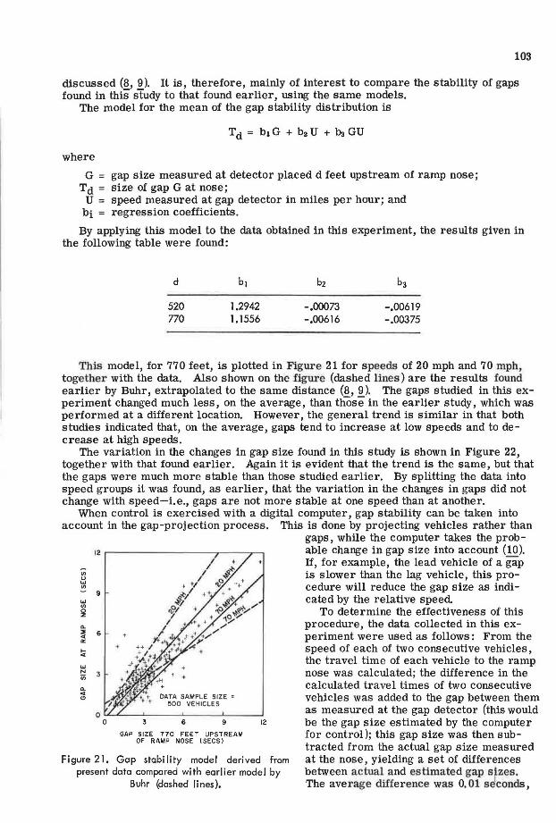
In summary, it can be said that, at the location studied, the average freewaydriver reduced his speed slightly as he approached the nose. This speed reduction does not appear to be greater at high speeds than

at low speeds. Most of the speed reduction appears to take place several hundred feet upstream from the nose. Since data were collected at only two points upstream from the nose, a reliable relationship between distance from the nose and average speed re­duction could not be established. The variability in speed changes among drivers does not seem to be greater at high speeds than at low speeds and does not seem to be in­fluenced by the distance studied. The speed-stability characteristics described may well be different at different geometric configurations and may be influenced by ramp demand.

Speed and Travel Time

In order to meter vehicles from a ramp into gaps on the freeway, the gaps neces­sarily have to be measured some distance upstream from the merging area. The travel time of this gap to the merge point then has to be estimated, using some speed mea­surement, in order to determine the exact moment at which to turn the ramp signal green. Since it has been shown that, on the average, speeds change somewhat between an upstream point and the nose of the ramp, it is of interest to investigate how this af­fects travel times and how the measured speed can best be used to estimate the travel time.

(/) 30

::J z j_ 20 ::i;il: <l::i; W- 10 a: ....... !> "'"' + ... ~~ 0

t~ -I"() ofil

"'"' '°<>. "(/) -20 l-w w Cl. (/) -30 0

20 40

SPEEO OF VEHICLE 520 FT OF RAMP NOSE (MPH)

60

UPSTREAM

0 50 100

FREQUENCY OF OCCURRENCE

Figure 18. Speed difference between ramp nose and point 520 feet upstream.

102

30

+} +

SAMPLE SIZE =500

20 40 60 SPEED OF VEHICLE 770 FT. UPSTREAM

OF RAMP NOSE (MPH)

-20

0 50 100 FREQUENCY OF

OCCURRENCE

Figure 19. Speed difference between ramp nose and a point 770 feet upstream.

Figure 20 shows the measured travel times plotted against the travel times estimated from the speeds measured 770 feet from the nose. Also shown is the line of no change. As expected, the actual travel times are generally higher than the calculated travel times. The higher travel times (low speeds) are generally more variable than the low travel times (high speeds), but this is to be expected since the same speed change would make a bigger difference in the travel time at low speeds than at high speeds. The data collected at 520 feet show essentially similar characteristics.

The fact lhat actual travel times were generally lower than calculated travel times can be compensated for by the control system. What cannot be compensated for is the variability of this difference. It is, therefore, of interest to investigate the distribution of the difference between actual travel times and travel time calculated from the mea­sured speeds. This distribution appears normal with a mean of 0.81 seconds and a standard deviation of 0.88 seconds, but does not provide a statistically significant fit with a normal distribution, mainly because of the high modal peak. The variability in these differences woW.d introduce an error into the accuracy with which the appearance of a gap in the merging area can be predicted. This error is such that almost 80 per­cent of the travel times could have been estimated to within 1 % seconds. In a control system, the speeds at the gap detector can be measured much more accurately than in this experiment, so that a better ac­curacy in predicting travel times can be obtained, if so desired.

The data measured at 520 feet showed a mean difference of 0.44 seconds with a standard deviation of 1. 04 seconds. From the data collected, it does not appear as if the variation in the difference increases with distance.

Gap Stability

The gap acceptance controller should estimate not only the time of arrival of a gap in the merging area, but also the size of the gap in the merging area based on its size as measured upstream. This esti­mation needs to take gap stability into ac­count. In an earlier work on gap sta­bility, models were developed and fitted to data collected at a particular site and the application to freeway control was

iii c z 0 u

"' !!!

...J

"' ~ a:

18

15

..... 12 c

"' a: ::>

"' ... llJ ::i; 9

...J ... ::> ..... u ...

+

+

+

+ + +

DATA SAMPLE SIZE = ~00

6"-~~-'-~~~-'---~~--''--~~~

6 9 12 15 18

TRAVEL TIME CALCULATED FROM SPEED AT 770 FT. (SECONDS)

Figure 20. Comparison of actual and estimated travel times over 770 feet.

103

discussed (8, 9). It is, therefore, mainly of interest to compare the stability of gaps found in this study to that found earlier, using the same models.

The model for the mean of the gap stability distribution is

where

G = gap size measured at detector placed d feet upstream of ramp nose; Td = size of gap G at nose;

U = speed measured at gap detector in miles per hour; and bi = regression coefficients.

By applying this model to the data obtained in this experiment, the results given in the following table were found:

d

520 770

1.2942 1.1556

-.00073 -.00619 -.00616 -.00375

This model, for 770 feet, is plotted in Figure 21 for speeds of 20 mph and 70 mph, together with the data. Also shown on the figure (dashed lines) are the results found earlier by Buhr, extrapolated to the same distance (8, 9). The gaps studied in this ex­periment changed much less, on the average, than those in the earlier study, which was performed at a different location. However, the general trend is similar in that both studies indicated that, on the average, gaps tend to increase at low speeds and to de­crease at high speeds.

The variation in the changes in gap size found in this study is shown in Figure 22, together with that found earlier. Again it is evident that the trend is the same, but that the gaps were much more stable than those studied earlier. By splitting the data into speed groups it was found, as earlier, that the variation in the changes in gaps did not change with speed-i.e., gaps are not more stable at one speed than at another.

When control is exercised with a digital computer, gap stability can be taken into account in the gap-projection process. This is done by projecting vehicles rather than

"' u "" "'

Q.

<I

"'

9

DATA SAMPLE SIZE • 500 VEHICLES

o~~~~~~~~~~~~-'

0 6 9

GAP SIZE 770 FEET UPSTREAM OF RAMP NOSE (SECS)

12

Figure 21. Gap stability model derived from present data compared with earlier model by

Buhr (dashed lines).

gaps, while the computer takes the prob­able change in gap size into account (10). If, for example, the lead vehicle of a gap is slower than the lag vehicle, this pro­cedure will reduce the gap size as indi­cated by the relative speed.

To determine the effectiveness of this procedure, the data collected in this ex­periment were used as follows: From the speed of each of two consecutive vehicles, the travel time of each vehicle to the ramp nose was calculated; the difference in the calculated travel times of two consecutive vehicles was added to the gap between them as measured at the gap detector (this would be the gap size estimated by the computer for control); this gap size was then sub­tracted from the actual gap size measured at the nose, yielding a set of differences between actual and estimated gap sizes. The average difference was O. 01 se1conds,

104

and the standard deviation was 0. 64 sec­onds. This represents a tremendous im -provement over the actual stability, as shown earlier in Figure 22. As a mat­ter of interest, the differences provided a statistically significant fit with a nor­mal distribution having the same mean and variance.

Total Travel and Total Travel Time

The objective of freeway control is often misstated as that of relieving free­way congestion or maximizing level of service. In actual fact, the objective is

2.0

"' M 1.0 0(1) o:­.. 0 z .. .... (I) o..._~~-'-~~--'-~~----''--~~-'-~

0 200 400 600 800

DISTANCE IN FEET

Figure 22. Standard deviation of gap stability distribution.

to optimize freeway operation or level of service. Just what this optimum is, is still open to question. Some authorities on the subject believe that optimum operation is reached when the flow smoothness is maximized (acceleration noise minimized). Others find strong arguments in favor of maximizing throughput-Le., moving the maximum amount of traffic in the minimum amount of time. However, whatever the criteria, it is necessary to have certain measures of effectiveness that can be evaluated in order to establish how well a certain freeway is operating or how well a certain control scheme is functioning. It is also necessary to know, or be able to establish, the optimum values of these measures of effectiveness.

The volume count, for example, is an excellent measure of effectiveness. Most traf­fic engineers have a good feel for the optimum volume count. Volume is, however, a point measure and does not necessarily reflect the operation in the entire system. Two measures that have often been used in the past are total travel (vehicle -miles)andtotal travel time (vehicle -hours).

The measure of total travel time has often been used with the implication that the system is improved if the total travel time is reduced (11). This is usually true as far as a congested freeway is concerned but need not necessarily always be true. To use a somewhat facetious example, by closing the freeway down completely, the total travel time can be reduced to zero.

Total travel time is related to total travel in somewhat the same way that density is related to volume. This relationship is illustrated in Figure 23 for a 2'/:i-mile section of the Gulf Freeway. The data were collected for a 1-hour period, during both morn­ing and afternoon control. If the freeway is congested, operation will be on the right­hand side of the curve. Under these conditions, it is true that the operation can be

24

iii

"' ...J i 18

'

"' ~ § 12

x ...J

"' ~ 0: .... 6

...J

~ 0 ....

+

TOTAL TRAVEL TIME (VEH -HOURS)

Figure 23. Operating -characteristic for a 2 Y2-mile section of the Gulf Freeway control system.

T,ss6o 0"'=54

500 600 700 800 900

" " 0 ,.,.

14

T3,TOTAL TRAVEL TIME (VEH. HRS)

- GAP ACCEPTANCE CONTROL (16 DAYSI ----DEMAND CAPACITY CONTROL (34 DAYS)

/

IS 16 17 18

T2 , TRAVEL(VEH MILES • 10-')

Figure 24. Operating characteristics on a 2Y2-mile section of the Gulf Freeway during the morning peak hour control

(7-8 a. m.).

19

105

improved by decreasing total travel time, provided that total travel also increases. Under free and stable flow conditions, op­eration will be on the left-hand side of the curve. In order to optimize operation under these conditions, total travel time has to be increased, provided that total travel also increases. Since the problem is actually a lack of demand, however, a freeway control system cannot force op­eration toward an optimum under these conditions. In some respects, therefore, this relationship can be considered as a warrant for control, because the opera­tion can be optimized if it falls on the right-hand portion of the curve but not on the left. However, the secondary objec­tive of freeway control is to improve merg­ing operations. This aspect is not re­flected by the relationship shown in Fig­ure 23. It is thought that this type of relationship will lead to warrants for the installation of a control system, but not necessarily to warrants for control, the difference being that the installation of a control system may be justified by the morning peak (or afternoon peak), while control of the other peak period may be justified by the improvements in merging operation, since the system then already exists.

In order to evaluate the effectiveness of two of the control systems presently in­stalled on the Gulf Freeway, the total travel and total travel times were accumulated for 1 hour during the morning under demand-capacity control and under gap-acceptance control. Demand-capacity control was exercised on all eight inbound ramps by analog controllers. Gap acceptance control was exercised by the digital computer on six of the inbound ramps while the remaining two ramps were under demand-capacity analog control. The results from 34 days of demand-capacity control and 16 days of gap­acceptance control (these days were selected because of the absence of accidents or incidents) were classified into frequency distributions and normal distributions fitted to them. The resulting normal distributions are shown in Figure 24. The total travel times fit the normal distributions quite well, but the total travel was not normally dis -tributed. The distributions in this case are used mainly for illustrative purposes. From the figures, it is clear that gap-acceptance control not only provided better op­eration, but provided consistently better operation as evidenced by the reduced stan­dard deviations. When the coordinates of the mean values from Figure 24 are compared with the operating characteristic of Figure 23, it can be seen that the gap­acceptance control results in operation very close to the optimum, while the demand­capacity control results in operation to the right (congested) of optimum.

APPLICATION TO FREEWAY CONTROL

The application of the characteristics derived in this paper to the design and opera­tion of a freeway control system has been discussed under each heading. These are by no means all the traffic information required to design, evaluate, and calibrate a control system. These characteristics merely begin to fill the void left by the rapid expansion of freeway control technology. It is hoped that the characteristics presented in this paper will be of some help to the traffic engineer charged with responsibility in this field and that they will prompt further investigations.

106

REFERENCES

1. Matson, T. M., Smith, W. S., and Hurd, F. W. Traffic Engineering. McGraw Hill, New York, 1955.

2. Traffic Engineering Handbook, Third Edition, 1965. 3. Knox, D. W. Merging and Weaving Operations in Traffic. Australian Road Re­

search, Vol. 2, No. 2, Dec. 1964. 4. Buhr, J. H. Mccasland, W. R, Carvell, J. D., and Drew, D. R Design of Freeway

Entrance Ramp Merging Control Systems. Research Report 504-3, Texas Trans­portation Institute, 1968.

5. Drew, D. R, Brewer, K. A., Buhr, J. H., and Whitson, R. H. Multilevel Approach to the Design of a Freeway Control System. Paper presented at the 48th Annual Meeting and included in this Record.

6. Drew, D. R, LaMotte, L. R., Wattleworth, J. A., and Buhr, J. H. Gap Acceptance in the Freeway Merging Process. Highway Research Record 208, p. 1-36, 1967.

7. Brewer, K. A., Buhr, J. H., Drew, D. R., and Messer, C. J. Ramp Capacity and Ser­vice Volume as Related to Freeway Control. Paper presented at 48th Annual Meeting and included in this Record.

8. Buhr, J. H. Freeway Entrance Ramp Merging Control Systems. Dissertation, Texas A&M University, Jan. 1967.

9. Buhr, J. H. Gap Stability and Its Application to Freeway Merging Control Systems. Traffic Engineering, March 1968.

10. Buhr, J. H., Drew, D. R, Gay, J. N., and Whitson, R.H. Design Specifications for Freeway Surveillance and Control Systems. Research Report RF 504-7, Texas Transportation Institute, 1968.

11. Wattleworth, J. A., Courage, K. G., and Carvell, J. D. An Evaluation of Two Types of Freeway Control Systems. Research Report 488-6, Texas Transportation Institute, 1968.