Traffic Analysis Toolbox Volume VII
51
Traffic Analysis Toolbox Volume VII: Predicting Performance with Traffic Analysis Tools PUBLICATION NO. FHWA-HOP-08-055 March 2008 Office of Operations 1200 New Jersey Avenue, SE Washington, DC 20590
Transcript of Traffic Analysis Toolbox Volume VII
Traffic Analysis Toolbox Volume VII:
Predicting Performance with Traffic Analysis Tools
PUBLICATION NO. FHWA-HOP-08-055 March 2008
Office of Operations1200 New Jersey Avenue, SE
Washington, DC 20590
harry.crump
Typewritten Text
harry.crump
Typewritten Text
harry.crump
Typewritten Text

Quality Assurance Statement The Federal Highway Administration (FHWA) provides high-quality information to serve Government, industry, and the public in a manner that promotes public understanding. Standards and policies are used to ensure and maximize the quality, objectivity, utility, and integrity of its information. FHWA periodically reviews quality issues and adjusts its programs and processes to ensure continuous quality improvement.

Technical Documentation Page
1. Report No.
FHWA-HOP-08-055
2. Government Accession No.
3. Recipient’s Catalog No.
4. Title and Subtitle Predicting Performance with Traffic Analysis Tools - Final Report
5. Report Date March 2008
6. Performing Organization Code
7. Authors T. Luttrell (SAIC), W. Sampson (University of Florida), D. Ismart (Louis Berger Group), D. Matherly (Louis Berger Group)
8. Performing Organization Report No.
9. Performing Organization Name and Address Science Applications International Corporation (SAIC) 1710 SAIC Drive McLean, VA 22102
10. Work Unit No. (TRAIS)
11. Contract or Grant No. DTFH61-06-D-00005; Task 25
12. Sponsoring Agency Name and Address United States Department of Transportation 1200 New Jersey Avenue, S.E. Washington, DC 20590
13. Type of Report and Period Covered
14. Sponsoring Agency Code HOTM
15. Supplementary Notes Mr. John Halkias (Task Manager)
Mr. Grant Zammit (Resource Center Technical Expert)
Mr. Barry Zimmer (COTR)
16. Abstract
This document provides insights into the common pitfalls and challenges associated with use of traffic analysis tools for predicting future performance of a transportation facility. It provides five in-depth case studies that demonstrate common ways to ensure appropriate results when using an microsimulation tool, and also includes “how to” material that allows users to address common challenges associated with microsimulation analysis.
Key Words Traffic Simulation Modeling, Traffic Analysis Tools, Microsimulation, Operational Analysis
18. Distribution Statement
No restrictions. This document is available to the public from: The National Technical Information Service, Springfield, VA 22161.
19. Security Classif. (of this report) Unclassified
20. Security Classif. (of this page) Unclassified
21.No of Pages 52
22. Price N/A
Form DOT F 1700.7 (8-72) Reproduction of completed page authorized.
PREDICTING PERFORMANCE WITH TRAFFIC ANALYSIS TOOLS
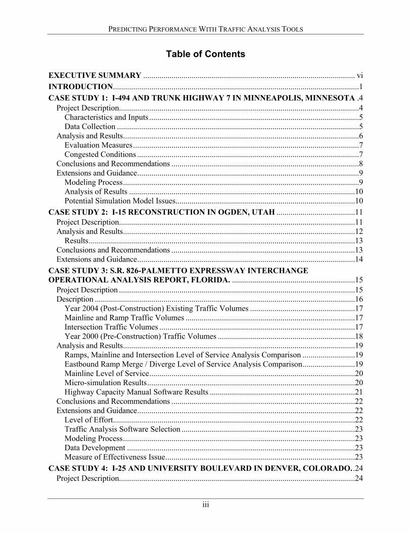
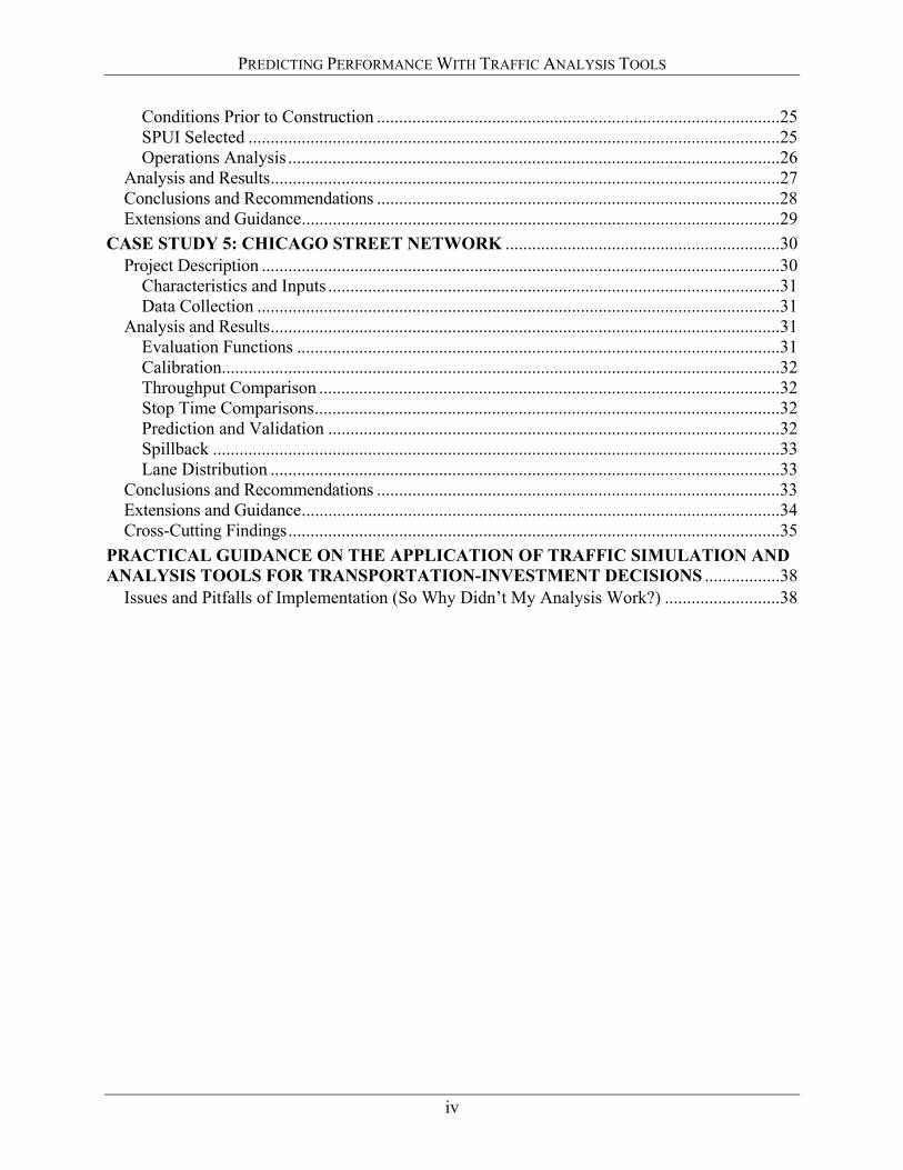
Table of Contents
EXECUTIVE SUMMARY ......................................................................................................... vi
INTRODUCTION..........................................................................................................................1
CASE STUDY 1: I-494 AND TRUNK HIGHWAY 7 IN MINNEAPOLIS, MINNESOTA .4 Project Description.......................................................................................................................4
Characteristics and Inputs ........................................................................................................5 Data Collection ........................................................................................................................5
Analysis and Results.....................................................................................................................6 Evaluation Measures................................................................................................................7 Congested Conditions ..............................................................................................................7
Conclusions and Recommendations .............................................................................................8 Extensions and Guidance..............................................................................................................9
Modeling Process.....................................................................................................................9 Analysis of Results ................................................................................................................10 Potential Simulation Model Issues.........................................................................................10
CASE STUDY 2: I-15 RECONSTRUCTION IN OGDEN, UTAH .......................................11 Project Description.....................................................................................................................11 Analysis and Results...................................................................................................................12
Results....................................................................................................................................13 Conclusions and Recommendations ...........................................................................................13 Extensions and Guidance............................................................................................................14
CASE STUDY 3: S.R. 826-PALMETTO EXPRESSWAY INTERCHANGE OPERATIONAL ANALYSIS REPORT, FLORIDA. .............................................................15
Project Description .....................................................................................................................15 Description .................................................................................................................................16
Year 2004 (Post-Construction) Existing Traffic Volumes ....................................................17 Mainline and Ramp Traffic Volumes ....................................................................................17 Intersection Traffic Volumes .................................................................................................17 Year 2000 (Pre-Construction) Traffic Volumes ....................................................................18
Analysis and Results...................................................................................................................19 Ramps, Mainline and Intersection Level of Service Analysis Comparison ..........................19 Eastbound Ramp Merge / Diverge Level of Service Analysis Comparison..........................19 Mainline Level of Service......................................................................................................20 Micro-simulation Results.......................................................................................................20 Highway Capacity Manual Software Results ........................................................................21
Conclusions and Recommendations ...........................................................................................22 Extensions and Guidance............................................................................................................22
Level of Effort........................................................................................................................22 Traffic Analysis Software Selection ......................................................................................23 Modeling Process...................................................................................................................23 Data Development .................................................................................................................23 Measure of Effectiveness Issue..............................................................................................23
CASE STUDY 4: I-25 AND UNIVERSITY BOULEVARD IN DENVER, COLORADO. .24 Project Description.....................................................................................................................24
iii
PREDICTING PERFORMANCE WITH TRAFFIC ANALYSIS TOOLS
Conditions Prior to Construction ...........................................................................................25 SPUI Selected ........................................................................................................................25 Operations Analysis ...............................................................................................................26
Analysis and Results...................................................................................................................27 Conclusions and Recommendations ...........................................................................................28 Extensions and Guidance............................................................................................................29
CASE STUDY 5: CHICAGO STREET NETWORK ..............................................................30 Project Description .....................................................................................................................30
Characteristics and Inputs ......................................................................................................31 Data Collection ......................................................................................................................31
Analysis and Results...................................................................................................................31 Evaluation Functions .............................................................................................................31 Calibration..............................................................................................................................32 Throughput Comparison ........................................................................................................32 Stop Time Comparisons.........................................................................................................32 Prediction and Validation ......................................................................................................32 Spillback ................................................................................................................................33 Lane Distribution ...................................................................................................................33
Conclusions and Recommendations ...........................................................................................33 Extensions and Guidance............................................................................................................34 Cross-Cutting Findings...............................................................................................................35
PRACTICAL GUIDANCE ON THE APPLICATION OF TRAFFIC SIMULATION AND ANALYSIS TOOLS FOR TRANSPORTATION-INVESTMENT DECISIONS .................38
Issues and Pitfalls of Implementation (So Why Didn’t My Analysis Work?) ..........................38
iv
PREDICTING PERFORMANCE WITH TRAFFIC ANALYSIS TOOLS
v
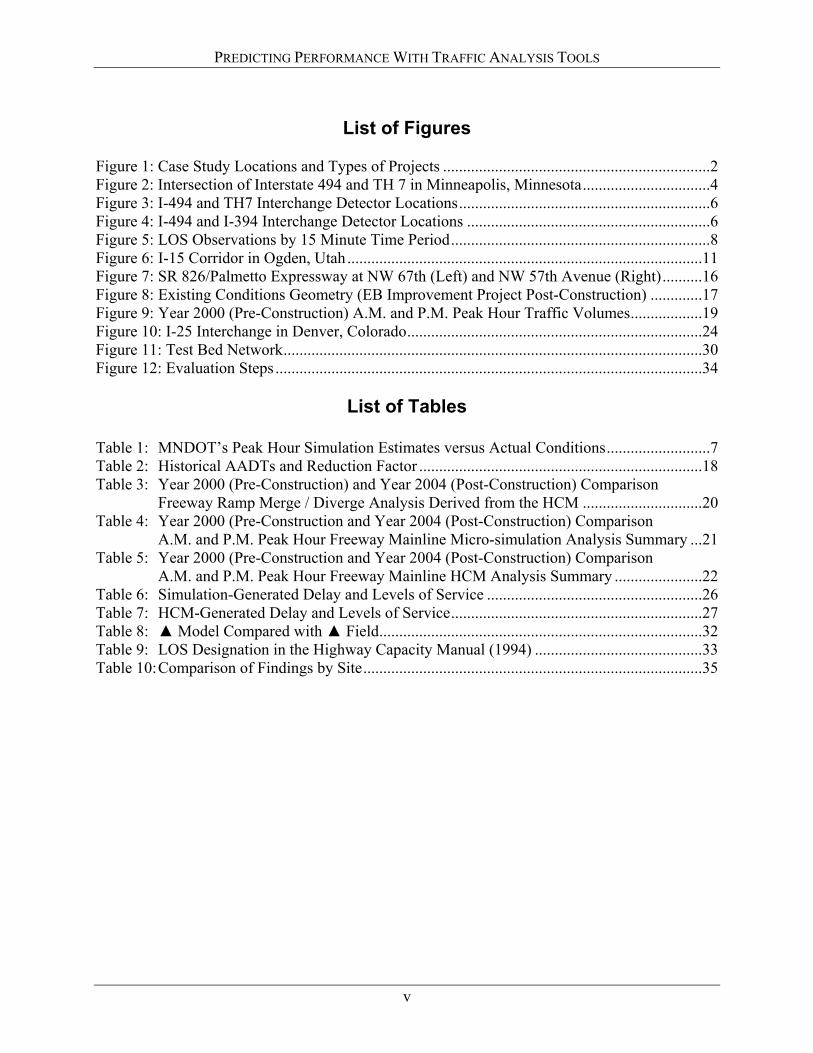
List of Figures
Figure 1: Case Study Locations and Types of Projects ...................................................................2 Figure 2: Intersection of Interstate 494 and TH 7 in Minneapolis, Minnesota................................4 Figure 3: I-494 and TH7 Interchange Detector Locations...............................................................6 Figure 4: I-494 and I-394 Interchange Detector Locations .............................................................6 Figure 5: LOS Observations by 15 Minute Time Period.................................................................8 Figure 6: I-15 Corridor in Ogden, Utah.........................................................................................11 Figure 7: SR 826/Palmetto Expressway at NW 67th (Left) and NW 57th Avenue (Right)..........16 Figure 8: Existing Conditions Geometry (EB Improvement Project Post-Construction) .............17 Figure 9: Year 2000 (Pre-Construction) A.M. and P.M. Peak Hour Traffic Volumes..................19 Figure 10: I-25 Interchange in Denver, Colorado..........................................................................24 Figure 11: Test Bed Network.........................................................................................................30 Figure 12: Evaluation Steps ...........................................................................................................34
List of Tables
Table 1: MNDOT’s Peak Hour Simulation Estimates versus Actual Conditions..........................7 Table 2: Historical AADTs and Reduction Factor .......................................................................18 Table 3: Year 2000 (Pre-Construction) and Year 2004 (Post-Construction) Comparison
Freeway Ramp Merge / Diverge Analysis Derived from the HCM ..............................20 Table 4: Year 2000 (Pre-Construction and Year 2004 (Post-Construction) Comparison
A.M. and P.M. Peak Hour Freeway Mainline Micro-simulation Analysis Summary ...21 Table 5: Year 2000 (Pre-Construction and Year 2004 (Post-Construction) Comparison
A.M. and P.M. Peak Hour Freeway Mainline HCM Analysis Summary ......................22 Table 6: Simulation-Generated Delay and Levels of Service ......................................................26 Table 7: HCM-Generated Delay and Levels of Service...............................................................27 Table 8: ▲ Model Compared with ▲ Field.................................................................................32 Table 9: LOS Designation in the Highway Capacity Manual (1994) ..........................................33 Table 10: Comparison of Findings by Site.....................................................................................35
PREDICTING PERFORMANCE WITH TRAFFIC ANALYSIS TOOLS
EXECUTIVE SUMMARY Traffic analysis tools play a critical role in prioritizing public investment in strategies employed by transportation professionals to relieve congestion. Use of traffic simulation and analysis tools has become the standard approach for evaluating transportation design alternatives, operational performance, Intelligent Transportation Systems (ITS) and traffic operations strategies. The purpose of this study is to assess and provide an understanding on how well simulation and traffic analysis tools predict performance, and identify elements and issues which practitioners should be aware of to effectively apply these tools. In order to support recommendations for use by practitioners, information was gathered and five locations were chosen for in-depth analysis. These sites include: 1) I-494 and Trunk Highway 7 in Minneapolis, Minnesota: Analysis of proposed freeway segment and interchange improvements. 2) I-15 Reconstruction in Ogden, Utah: Analysis of maintenance of traffic and reconstruction closure scenarios. 3) S.R. 826-Palmetto Expressway Off-Ramps near Miami, Florida: Analysis of proposed off-ramp improvements and the addition of an auxiliary lane. 4) I-25 and University Boulevard in Denver, Colorado: Estimation of performance of replacing a full cloverleaf interchange with a single point urban interchange (SPUI). 5) Traffic Signal Network in Chicago, Illinois: Study of key issues in the validation of a microsimulation analysis of a complex arterial network signal timing project. The five cases were selected to test a variety of software model tools across a range of applications and settings, illustrative of problems as well as best practices, to derive lessons learned. During these investigations, much was learned that increases the understanding of current practice and provides insights into improving future analyses. The summary and recommendations at the end of this report discuss examples of lessons learned, and how the modeling process can account for the types of modeling challenges identified. The information presented in the case studies, along with conclusions drawn from the analyses and experience of the authors, are the foundation for a practical set of guidelines and suggestions for overcoming common shortcomings, unreliable assumptions and similar problems. The checklist included as Attachment 1 provides a summary guide to a host of issues that contribute to deviations between simulations and observed conditions.
vi

PREDICTING PERFORMANCE WITH TRAFFIC ANALYSIS TOOLS
INTRODUCTION Traffic analysis tools play a critical role in prioritizing public investment in strategies employed by transportation professionals to relieve congestion. Use of traffic simulation and analysis tools has become the standard approach for evaluating transportation design alternatives, operational performance, Intelligent Transportation Systems (ITS) and traffic operations strategies. These tools are being utilized by agencies to assess the performance of existing operations as well as the prediction of future operations. As reliance on these tools increases it is critical to understand how well they predict performance under actual as well as assumed conditions. Purpose The purpose of this study is to assess and provide an understanding on how well simulation and traffic analysis tools predict performance, and identify elements and issues which practitioners should be aware of to effectively apply these tools. Often, misapplication of a tool can change the results enough to significantly impact the decision making process. Since the modeling process is often used to support investment decisions on higher cost projects, misapplication of a tool might result in significant cost implications. Rationale for the Cases Information was gathered on more than 20 potential case study locations. In order to determine the sites that would provide the best information, site selection criteria were developed and applied. These criteria include the following: Availability of “after” data, preferably sites where an “after” study was performed Diversity in traffic analysis tools used (may include more than one) Diversity in type of improvement or operational strategy modeled or proposed Geographic dispersion across sites Facility type Location type (e.g., rural, urban, downtown) Location characteristics (e.g., percent of local traffic versus through traffic, percent trucks, percent
commuter traffic) Typical volume/capacity or level of congestion Agency’s experience with the use of traffic analysis tools Information Gathering Once the site selection criteria was applied and a list of the five top sites was generated, contact was made with local project representatives (often both in the public and private sector) to extract information on the potential case study. For sites with “after” studies, summary reports were gathered to assess any completed comparisons of model results with actual field conditions. For sites where the strategy or construction was already implemented, investigations were performed into the potential for data gathering at the site to facilitate analysis of field conditions. Where appropriate,
1

PREDICTING PERFORMANCE WITH TRAFFIC ANALYSIS TOOLS
2
agencies provided actual files from the tool used. These files were analyzed to support the conclusions drawn within this report. Scope of Each Case Study This study was carried out through in-depth discussions with traffic operations practitioners who had relied on a transportation model to assist them in designing a technical solution to a traffic engineering problem, only to find that the reality of the traffic and operation of the project was somewhat or significantly different from that projected by the model. More than 20 potential cases were initially evaluated and narrowed to five cases for in-depth analysis. The five cases are shown in Figure 1 and briefly described below.
Figure 1: Case Study Locations and Types of Projects
1) I-494 and Trunk Highway 7 in Minneapolis, Minnesota: Modeling for the widening of I-494 from 4-lanes to 6-lanes From Valley Creek Road to TH 55 in the west metro area. 2) I-15 Reconstruction in Ogden, Utah: Investigation of various I-15 reconstruction closure scenarios to model and quantify the impact on travelers during the project. 3) S.R. 826-Palmetto Expressway Off-Ramps near Miami, Florida: Documentation of the operations of off-ramp improvements and the addition of an auxiliary lane.
Chicago, IL: Arterial Network Signal Timing Improvements
Miami, FL: Interchange Operational Analysis
Denver, CO: Single Point Urban Interchange Upgrade Analysis
Ogden, UT: Modeling of Construction Alternatives
Minneapolis, MN: Freeway and Interchange Upgrade Analysis

PREDICTING PERFORMANCE WITH TRAFFIC ANALYSIS TOOLS
4) I-25 and University Boulevard in Denver, Colorado: Estimation of performance of replacing a full cloverleaf interchange with a single point urban interchange (SPUI). 5) Traffic Signal Network in Chicago, Illinois: Study of key issues in the validation of a microsimulation analysis of a complex arterial network signal timing project. The five cases were selected to test a variety of software model tools across a range of applications and settings, illustrative of problems as well as best practices, to derive lessons learned. FHWA’s Traffic Analysis Toolbox provides information on the process for carrying out a microsimulation analysis project. Some of the processes used in each case study listed are very similar to the process outlined in Volume 3 of the Traffic Analysis Toolbox; however, formal site-specific processes for modeling and simulation may not be as clearly defined as the FHWA-developed process. Practitioners from all the sites studied and highlighted in this document used some or most elements of the Toolbox process according to their own established procedures and the procedures required for the particular software that was employed, sometimes without specific reference to a defined process. Many of the elements of the process are clear to users and must be applied to perform a study, while others, and the appropriate techniques for application, may not be. Each case study that employed use of an appropriate tool that leads to the metric of Levels of Service (LOS) modeled conditions during the worst 15 minute period (peak flow rate). The cases that used microsimulation went well beyond the peak 15 minute flow rate typically used for LOS, and usually encompassed multiple time periods including the peak hour and often the peak period, as discussed in the case studies. Additional metrics that were analyzed in one or more of the case studies included queuing, delay (signals), density (freeways), bottlenecking, spillback, following patterns and lane distribution, and crash rates. During these investigations, much was learned that increases the understanding of current practice and provides insights into improving future analyses. The summary “Issues of Implementation” at the end of this report discusses examples of lessons learned, and how the user can anticipate / adjust / compensate for the types of modeling challenges identified (“So what should a user do?”). These cases and summary are the foundation for a (forthcoming?) practical set of guidelines and suggestions for typical studies to overcome common shortcomings, unreliable assumptions similar problems.
3

PREDICTING PERFORMANCE WITH TRAFFIC ANALYSIS TOOLS
CASE STUDY 1: I-494 AND TRUNK HIGHWAY 7 IN MINNEAPOLIS, MINNESOTA
Project Description In 2006, the Minnesota Department of Transportation (MNDOT) planned, designed, and constructed an expanded section of Interstate 494 in Minneapolis. The project involved widening I-494 from 4-lanes to 6-lanes From Valley Creek Road to TH 55 in the west metro area. To support the analysis of alternatives, MNDOT used a traffic simulation tool to model future conditions along I-494 along with interchanges. For one specific interchange, I-494 and Trunk Highway (TH) 7, MNDOT modeled two build scenarios including a full cloverleaf interchange and a partial cloverleaf interchange, along with a no-build scenario. The area of study is shown in Figure 2. The interchange is located southwest of Minneapolis in a suburban area.
Figure 2: Intersection of Interstate 494 and TH 7 in Minneapolis, Minnesota
4

PREDICTING PERFORMANCE WITH TRAFFIC ANALYSIS TOOLS
5
At the time of the analysis, the existing interchange was a full cloverleaf. MNDOT was concerned with the potential impacts on the loops from the freeway widening project and gave additional scrutiny to the I-494/TH7 interchange.
ar design timeframe. MNDOT opened the upgraded interchange to traffic on August 31, 2006.
ed to emonstrate peak period performance better than the peak 15 minute measures often used.
urated conditions for the freeway to see how well the analysis predicted ctual field conditions.
Cookbook: Discover the Magic of Data Extraction” based on e following MnDOT guidance:
days with traffic incidents during the AM or PM peak period (7 to 8 AM and 4
torm resulting in visibility of ¼ mile or less, smoke or haze, blowing snow, and tornado).
Characteristics and Inputs
The planning and design of the project included a simulation model analysis for year opening (2006) and the 20 ye
Data Collection
MNDOT maintains an electronic repository of data for all freeways in the Twin Cities Metropolitan area. MNDOT archives the data and provides public access to the data via a website. The system archives volume, speed, headway, and occupancy data from loop detectors and calculates metrics such as density and flow rate. These advanced metrics are intendd Data were downloaded from the system for analysis and comparison with the simulation model output and results to test how well the simulation process performed. We focused the analysis on freeway and loop operational characteristics for the I-494/TH7 interchange area. Since the metrics showed acceptable levels of service, we also chose one additional location where the model predicted oversata To this case study assessment, after data during a period from September 2006 through June 2007 was obtained. This timeframe was selected based on data guidelines from MnDOT’s publication titled “Data Extractionth
Eliminate weekends, Mondays, and Fridays Eliminate holidays and the days before and after holidays Eliminate bad weather days (days with snow or more than 0.20 inches of rainfall) Eliminate
to 5 PM) Eliminate days with special weather incidents (e.g., fog or mist, fog reducing visibility to
¼ mile or less, thunder, ice pellets, hail, freezing rain or drizzle, duststorm or sands
Weather information was also obtained for the Twin Cities area via http://www.weather.gov, combined with an inquiry about historical traffic incident information to identify any effects due to recurring and nonrecurring incidents. MnDOT recently phased out the Metro Incident Selection Tool (MIST); therefore, incident archives were not available for analysis. While incidents may have occurred on some of the analysis days, no incidents were accounted for due to the lack of data.
PREDICTING PERFORMANCE WITH TRAFFIC ANALYSIS TOOLS
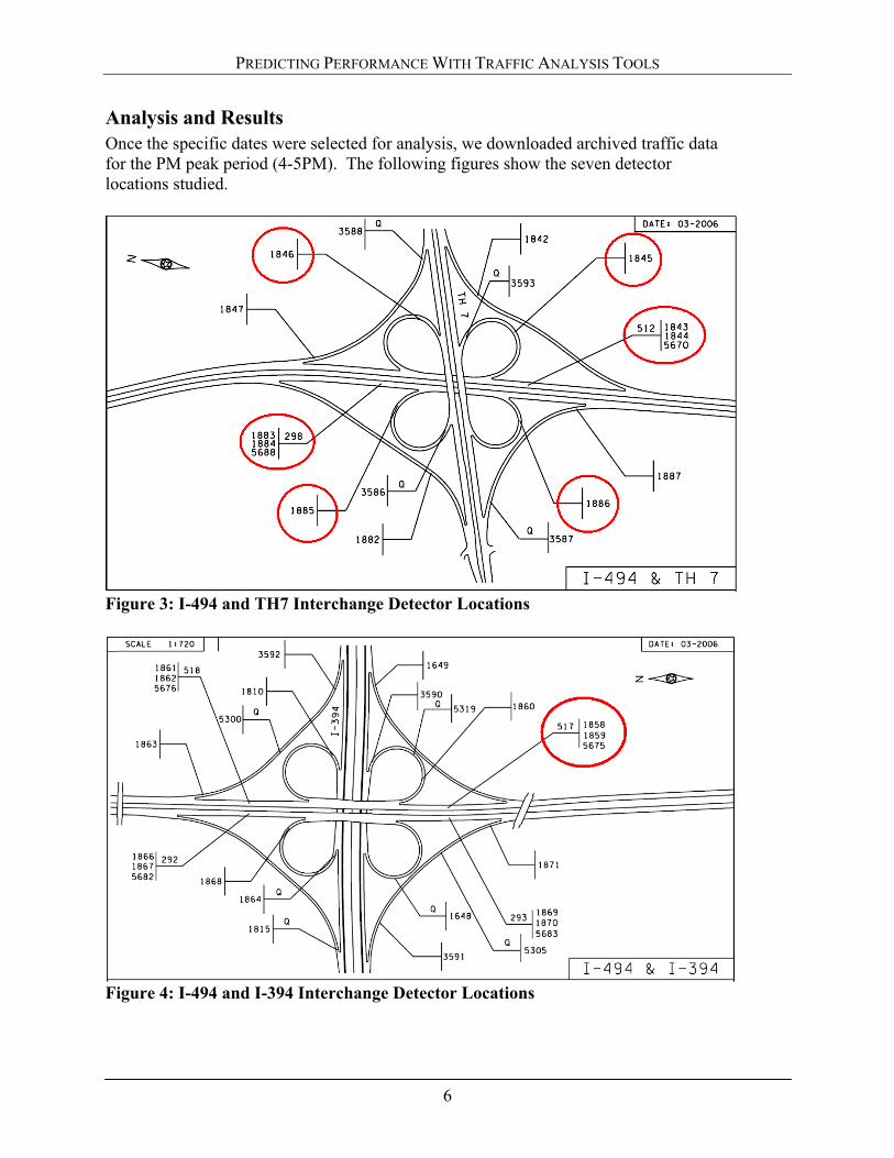
Analysis and Results Once the specific dates were selected for analysis, we downloaded archived traffic data for the PM peak period (4-5PM). The following figures show the seven detector locations studied.
Figure 3: I-494 and TH7 Interchange Detector Locations
Figure 4: I-494 and I-394 Interchange Detector Locations
6

PREDICTING PERFORMANCE WITH TRAFFIC ANALYSIS TOOLS
Evaluation Measures
Results for simulated throughput were compared with actual flow rates. The average field measured flow rate was consistently higher than the simulated throughput due in part to an issue with a previous version of this model in overestimating impacts from bottlenecks. Additionally, travel demand data may have been underestimated by the planning model used, especially since true “demand” is higher than loop detectors can count – given that they only see departure volumes – during congested conditions. Since this project was a partial reconstruction of I-494, the freeway lane configuration reduces from six to four lanes further downstream compared with the configuration prior to construction During the original analysis and prior to construction, field observations by MnDOT’s analysis team highlighted issues with the operating conditions on each ramp due to the constrained right-of-way. The simulated speeds for the ramps were fairly similar to the actual detector speeds, with the actual speeds slightly higher in the field for 5 of the 7 study locations. The model results helped MnDOT better understand the projected operating conditions and the speed profiles helped them decide to expand the existing full clover leaf design within the constrained right of way compared with the partial clover leaf alternative. Increasing the volumes to try and predict true demand through sensitivity analysis may have been helpful in determining break points for acceptable versus unacceptable operating conditions. Table 1 compares simulated measures with actual field conditions. Since the ramp loop detectors are located at the mid points of the ramps, density and LOS do not apply for the ramps. Influences from merge and diverge areas were accounted for in the simulation but not directly reported as they would be from a Highway Capacity Analysis. All of the ramp roadways have peak hour volumes that are below capacity. . Table 1: MNDOT’s Peak Hour Simulation Estimates versus Actual Conditions
Simulation Statistics Average Field Conditions
Location Through-
put Speed Density LOS
Through-put
Speed Density LOS
NB I-494 Off Ramp 518 29 N/A N/A 517 25 N/A N/A
SB I-494 Off Ramp 323 29 N/A N/A 249 27 N/A N/A I494 On Ramp from EB TH7
723 20 N/A N/A 613 25 N/A N/A
I494 On Ramp from WB TH7
82 22 N/A N/A 66 26 N/A N/A
SB I494 Mainline 4221 67 14 B 3589 75 16 B
NB I494 Mainline 5131 62 16 B 4629 73 22 C
NB I494 at I394 5544 42 58 F 4302 65 29 D
Congested Conditions
The freeway segment northbound on I494 at the I394 interchange was selected to test one location that MnDOT projected to have failing operating conditions. As shown in Table 1, the average actual density for this segment was 29 passenger cars per hour per lane (pcphpl), while the model predicted 58 pcphpl. However, several 15 minute time periods of actual field data showed a density greater than 45, indicating LOS F based on the Highway Capacity Manual. The model also included consideration of truck traffic impacts based on truck operating parameters that differ from those of passenger cars, and the MnDOT data archives also account for truck percentages. In this case, the
7

PREDICTING PERFORMANCE WITH TRAFFIC ANALYSIS TOOLS
8
model results helped MNDOT better understand and enhance the justification for the need to widen the freeway, even though high densities were projected for the widened section in the future as well. The six lane section would enhance traffic operations compared with the four lane section. Additionally, this area would likely be influenced by the nearby downstream weaving segment which could involve a different analysis to determine operating performance.
Figure 5 highlights the LOS categories within which each individual 15 minute density value falls, as observed from actual field conditions. The model’s average density was higher than the field-measured average density. However, several periods with LOS F were observed. As MnDOT successfully proved, agencies should understand the level of detail being analyzed to ensure a full understanding of the operating conditions of the facility. Often, temporal descriptions of results are needed to help decision makers understand operations. For example, LOS F should be accompanied by the time period the LOS is observed, how long it lasts, and if an improvement reduces density or delay but does not change level of service.
Conclusions and Recommendations The purpose of this analysis was to analyze how the application of a micro-simulation tool provided support to decision makers and determine how well the tool predicted future operating conditions for the freeway and interchange and how it influenced the decision. Although right of way constraints and time limitations for reconstruction drove the decision to keep the existing loops, use of the model enhanced the decision making process. The analysis adequately predicted future freeway operating conditions and overall helped MNDOT understand the potential impacts from the freeway reconstruction project. Variation in results for several measures may have mainly been due to error in demand projections based on expanded capacity. Based upon discussions with the Minnesota DOT team, they believe that a sensitivity analysis should be built in to determine, based on the level of confidence in the data projections, the point at which additional traffic may make the facility reach congested conditions or conditions degraded below a desired threshold.
Figure 5: LOS Observations by 15 Minute Time Period
0 10 20 30 40 50 60 70 80 90
100
LOS A LOS B LOS C LOS D LOS E LOS F
Level of Service Bins
Num
ber o
f 15-
min
ute
Obs
erva
tions
NB I494 at I394

PREDICTING PERFORMANCE WITH TRAFFIC ANALYSIS TOOLS
Extensions and Guidance
The following observations and guidance are offered as a result of the analysis and discussions with project personnel.
Level of Effort – Being a significant corridor level analysis (this report focuses mainly on one interchange within the larger study), the level of effort for this particular simulation project is estimated to be approximately 1500 person-hours over three months. This level of effort is based on users with significant simulation modeling experience and who have access to an excellent data repository from which data can be extracted electronically. Additionally, users had access to data processing tools, such as a Visual Basic interface tool developed prior to this study that processes simulation output files and organizes the output data into a spreadsheet for ease of analysis and reporting. A similar study with less experienced modelers and more time consuming data collection and data gathering would expand the level of effort beyond what is estimated for this study.
Needs that would add level of effort to this particular magnitude of project include:
Field data collection or data gathering from another agency such as planning data from a Metropolitan Planning Organization (MPO).
Additional time needed for less experienced users to familiarize themselves with the model.
Additional time needed for any expanded sensitivity analyses that may be needed to determine the future break point demand for a facility. This type of analysis would enhance the results and decision making process.
Setting up the model and coding the geometrics normally takes less time than data gathering and input, especially without links to electronic data repositories such as the MNDOT data tools website. Users should allow for adequate time to gather data.
Tools can be developed, similar to the one mentioned in this case, to automate data input and output processing to save time and cost over multiple simulation projects. Early investments may be needed to lower future level of effort.
Modeling Process
Users should use simulation modeling to get verifiable results, not simply a set of quantified results from a completed analysis. The results should be reasonable and based on model calibration. Much of the process FHWA has published for using simulation models was developed in parallel with the process used by MnDOT. One area that is evolving for MnDOT is model calibration. With added experience, modelers can enhance their understanding of the parameters that, when altered, will have the most impact on the results.
Model results should be used to support decision-making processes and therefore need to be adequately communicated to decision-makers. Additionally, users should not simulate every idea proposed, but should use discussion and other tools to narrow the list to a few alternatives that are the most promising and that can best support decision-making.
9

PREDICTING PERFORMANCE WITH TRAFFIC ANALYSIS TOOLS
Analysis of Results
Users should be careful when comparing information across traffic analysis tools. For example, MNDOT used simulation-produced freeway densities within the Highway Capacity Manual’s level of service thresholds. FHWA does not promote nor encourage the reporting of LOS based on an alternative tool’s results due to the differences in the way these metrics are calculated. The HCM uses passenger-car equivalents and peak flow rates to determine density, and the level of service thresholds were designed for use with this particular procedure for calculating density. Results should be displayed in an appropriate way to allow decision-makers to view the results within the context they were designed for. Simulations should further define latter (later??) steps in the process.
Potential Simulation Model Issues
Since this analysis was performed in 2002, MNDOT used an older version of the simulation model than is currently available. The older version of the model had difficulties in predicting impacts from lane drops on freeways. This issue has been alleviated in the current version of the model. However, the earlier model’s tendency to overestimate impacts from lane drops and underestimate the ability of the traffic stream to recover from such congested conditions may have been responsible for the model overestimating the congestion and underestimating the throughput compared with the field data. Users should be familiar enough with potential issues to properly calibrate the model and should validate the findings as much as possible to ensure accurate results.
10
PREDICTING PERFORMANCE WITH TRAFFIC ANALYSIS TOOLS
CASE STUDY 2: I-15 RECONSTRUCTION IN OGDEN, UTAH
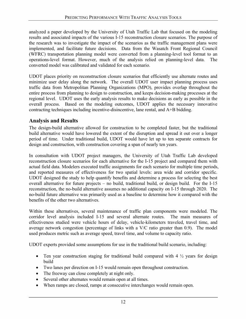
Project Description The Utah Department of Transportation (UDOT) uses a program-level traffic analysis framework called “User Impact Planning” to help facilitate implementation of construction programs and to help determine operational treatments during construction to alleviate impacts. Modeling helps UDOT better understand future operational characteristics and allows for enhanced planning activities. For example, the Statewide Transportation Improvement Program (STIP) may have multiple projects proposed for the same year. The UDOT modeling program helps decision-makers determine the timing for the construction projects at the system level and helps with scheduling decisions and letting timeframes. The UDOT process includes three stages, where the second stage involves planning level analysis to evaluate three alternatives – no build, traditional build, and fast track design-build. The analysis at this level includes quantitative estimates of measures of effectiveness including total vehicle hours of delay per alternative. The trade off between traditional build and design build lies in the typically slow progress with moderate impacts versus fast progress with shorter, more intense impacts, respectively. In this case, the design build alternative significantly compressed the construction schedule.
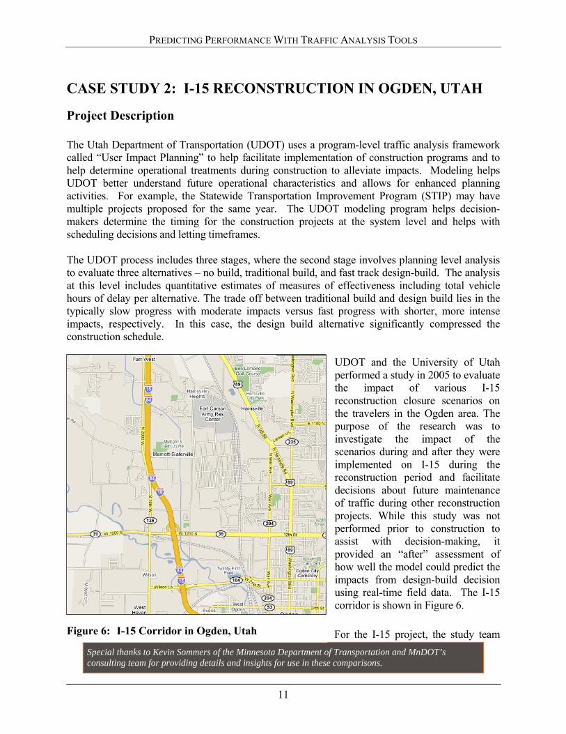
UDOT and the University of Utah performed a study in 2005 to evaluate the impact of various I-15 reconstruction closure scenarios on the travelers in the Ogden area. The purpose of the research was to investigate the impact of the scenarios during and after they were implemented on I-15 during the reconstruction period and facilitate decisions about future maintenance of traffic during other reconstruction projects. While this study was not performed prior to construction to assist with decision-making, it provided an “after” assessment of how well the model could predict the impacts from design-build decision using real-time field data. The I-15 corridor is shown in Figure 6.
Figure 6: I-15 Corridor in Ogden, Utah For the I-15 project, the study team
Special thanks to Kevin Sommers of the Minnesota Department of Transportation and MnDOT’s consulting team for providing details and insights for use in these comparisons.
11
PREDICTING PERFORMANCE WITH TRAFFIC ANALYSIS TOOLS
analyzed a paper developed by the University of Utah Traffic Lab that focused on the modeling results and associated impacts of the various I-15 reconstruction closure scenarios. The purpose of the research was to investigate the impact of the scenarios as the traffic management plans were implemented, and facilitate future decisions. Data from the Wasatch Front Regional Council (WFRC) transportation planning model were converted from a planning-level tool format to an operations-level format. However, much of the analysis relied on planning-level data. The converted model was calibrated and validated for each scenario. UDOT places priority on reconstruction closure scenarios that efficiently use alternate routes and minimize user delay along the network. The overall UDOT user impact planning process uses traffic data from Metropolitan Planning Organizations (MPO), provides overlap throughout the entire process from planning to design to construction, and keeps decision-making processes at the regional level. UDOT uses the early analysis results to make decisions as early as possible in the overall process. Based on the modeling outcomes, UDOT applies the necessary innovative contracting techniques including incentive-disincentive, lane rental, and A+B bidding.
Analysis and Results The design-build alternative allowed for construction to be completed faster, but the traditional build alternative would have lowered the extent of the disruption and spread it out over a longer period of time. Under traditional build, UDOT would have let up to ten separate contracts for design and construction, with construction covering a span of nearly ten years. In consultation with UDOT project managers, the University of Utah Traffic Lab developed reconstruction closure scenarios for each alternative for the I-15 project and compared them with actual field data. Modelers executed traffic assignments for each scenario for multiple time periods, and reported measures of effectiveness for two spatial levels: area wide and corridor specific. UDOT designed the study to help quantify benefits and determine a process for selecting the best overall alternative for future projects – no build, traditional build, or design build. For the I-15 reconstruction, the no-build alternative assumes no additional capacity on I-15 through 2020. The no-build future alternative was primarily used as a baseline to determine how it compared with the benefits of the other two alternatives. Within these alternatives, several maintenance of traffic plan components were modeled. The corridor level analysis included I-15 and several alternate routes. The main measures of effectiveness studied were vehicle hours of delay, vehicle-kilometers traveled, travel time, and average network congestion (percentage of links with a V/C ratio greater than 0.9). The model used produces metric such as average speed, travel time, and volume to capacity ratio. UDOT experts provided some assumptions for use in the traditional build scenario, including:
Ten year construction staging for traditional build compared with 4 ½ years for design build
Two lanes per direction on I-15 would remain open throughout construction. The freeway can close completely at night only. Several other alternates would remain open at all times. When ramps are closed, ramps at consecutive interchanges would remain open.
12
PREDICTING PERFORMANCE WITH TRAFFIC ANALYSIS TOOLS
13
Some planning tools account for the impacts of signalized intersections on arterials by reducing capacity on those links in the network. A micro simulation analysis tool will produce more realistic delay values compared with planning tools. In using any level of tool (planning versus simulation),the availability of high quality travel demand data is important to producing the best analysis results.
Construction time for a single interchange would last at least two years (three years for a major junction or pair of interchanges).
The modeling exercise included five time periods: AM peak (6-9am), PM peak (3-6pm), daytime period (9am-3pm), evening period (6-10pm), and the nighttime period (10pm-6am). The study focused on the average V/C ratios for the PM peak hour only.
Results
The model estimated savings of approximately 60 million hours of delay by using Design Build versus Traditional Build, for a fifteen year analysis period. Vehicle kilometers of travel did not differ significantly between the three alternatives; however, the model estimated that the no-build alternative would experience significant congestion and VKT would likely increase as motorists seek alternate routes that may increase their trip length. The design-build alternative proved to be the best alternative based on this “after” analysis. Assessing the field data, it was confirmed that the analysis failed to estimate acceptably accurate V/C ratios on the corridors. Correlation coefficients were high at the average daily traffic comparison level, but when the analyst developed correlation coefficients based on data at the peak hour level they were much lower. Ultimately, however, the analysis produced data that matched fairly closely with the local MPO travel demand forecasts. The other corridor-specific measures were found to be comparable with the field observations. The model also showed a lack of ability to reproduce accurate saturation rates for the major arterials. This inaccuracy in estimating saturation rates is inherent in the limitations of transportation planning models. The planning models must be designed to accurately distribute traffic demand over all links in the real street network. Additionally, the model included several different types of facilities including freeways, major and minor arterials, and collector roads. In addition, transportation planning models rarely include signals in their modeling procedures.
Conclusions and Recommendations The purpose of this analysis was to highlight some of the issues experience by UDOT in assessing traffic control alternatives for a major reconstruction project. Since data were already available in analyzed format, the study team expanded on existing findings to provide insights to agencies interested in similar analysis processes. The major finding from this study lies in the potential limitation of planning tools to accurately predict future demand and volume to capacity ratios. The University of Utah study concluded that either the arterial capacities or throughput estimates are overly reduced by the model, or the demand on the links in the model’s network is overestimated. The University study also concluded that LOS values would likely be much higher than values obtained from a micro simulation or signal optimization tool, further supporting the finding that users should be careful in how they compare results, as they may not

PREDICTING PERFORMANCE WITH TRAFFIC ANALYSIS TOOLS
be directly comparable across different models or simulation tools. Other results from the study are more or less comparable with the field observations.
Extensions and Guidance The issue with V/C ratios (discussed under “Results”) was due in part to limitations in the use of a transportation planning application with a desired end result being a detailed operational analysis of traffic patterns. Agencies are often faced with the challenge of predicting future traffic patterns with enough accuracy to evaluate operational-level conditions, even though the tool used may be designed mainly for the planning level. The task of determining how well traffic control alternatives will function is especially difficult, given the need to have highly accurate demand information. Additionally, a sensitivity analysis could be used to determine break points for congested conditions by providing a range of potential V/C ratios that might be expected, especially due to likely potential error in demand forecasts. At the planning and operations levels, model networks should be large enough to include all traffic that may potentially be impacted by construction. For example, UDOT developed a network model that included major alternate routes to I-15. State agencies should also coordinate with local agencies as appropriate to ensure appropriate network coverage and to gather appropriate data to use within the model. Consequently, UDOT owns and maintains many of the alternate routes, including signalized arterials that might likely be owned by cities or counties in other states. Since a majority of the urban population in Utah lives along the I-15 corridor and Wasatch Front, the model developed in this project will be extremely useful for future analysis without the original level of effort required to initially build the model. The overall study in this case cost $93,000, with approximately 75% of the total used in setting up the model and the remainder used in analyzing the results. During the period of performance for the original study, the Utah Traffic Lab was being constructed and therefore ultimately provided the University with direct traffic data links to the UDOT traffic management system. As with the MNDOT example, access to electronic data in near real-time was a convenient and cost-saving measure for this study.
Special thanks to Doug Anderson, UDOT and Aleksandar Stevanovic of the University of Utah Traffic Lab for providing details and insights for use in these comparisons.
14

PREDICTING PERFORMANCE WITH TRAFFIC ANALYSIS TOOLS
CASE STUDY 3: S.R. 826-PALMETTO EXPRESSWAY INTERCHANGE OPERATIONAL ANALYSIS REPORT, FLORIDA. NW 57th and NW 67th Avenues Eastbound Off-Ramps
Project Description Case Example 3 documents the comparative findings of pre- and post-construction operational level of service for the eastbound (EB) off-ramps and the auxiliary lane along the SR 826-Palmetto Expressway east-west corridor for the NW 67th and NW 57th Avenues interchanges. The purpose of this ‘before and after’ analysis was to provide the Florida DOT with a detailed analysis that documents the improved traffic operations (density and level of service) due to the eastbound off-ramp improvements and the construction of an eastbound auxiliary lane. The eastbound interchange improvement project began on January 22, 2001 and was completed March 20, 2002. FDOT conducted the study to assist them in determining if similar ramp and auxiliary lane improvements for the westbound direction would be warranted. The eastbound SR 826 Palmetto Expressway ‘before and after’ study was initiated due to the Florida DOT design team completing an Interchange Operational Analysis Report (IOAR) which was submitted to Department in December 2004 for the westbound (WB) off-ramps at the NW 67th and NW 57th Avenues interchanges. The report recommended construction of a continuous WB auxiliary lane, and widening of the off-ramps to two lanes, along with operational improvements to the intersections. The Scoping Committee requested a study of the recently improved eastbound off ramps, at NW 67th and 57th Avenues, in order to verify whether the objectives of that project have been accomplished. The recommended improvements included widening of the off-ramps and adding a continuous auxiliary lane between both interchanges. Due to the similarities in configuration and recommendations, it was decided that an evaluation of before and after conditions in the EB direction (field review and microsimulation comparisons) would be the best way to establish whether the proposed WB improvements in the IOAR (December 2004) are sound and worth pursuing. Although the eastbound interchange improvements existed when the ‘before and after’ study was initiated, the microsimulation analysis was conducted to quantify the eastbound ramp improvements contribution to the SR 826 Palmetto Expressway operations. Growth in the Expressways traffic as well as not having field data prior to the construction of the eastbound interchange improvements made it difficult to assess the extent of the operational improvements by field observation alone. The comparison was conducted by applying a microsimulation software analysis to determine what the changes in the level of service would be due to interchange improvements. The interchange improvements were also evaluated by using a deterministic Highway Capacity Manual software package. A comparison was made between the final analysis of the microsimulation software, the Highway Capacity Manual procedure, and the actual condition. The EB interchange improvement project began January 22, 2001 and was completed March 20, 2002.
15
PREDICTING PERFORMANCE WITH TRAFFIC ANALYSIS TOOLS
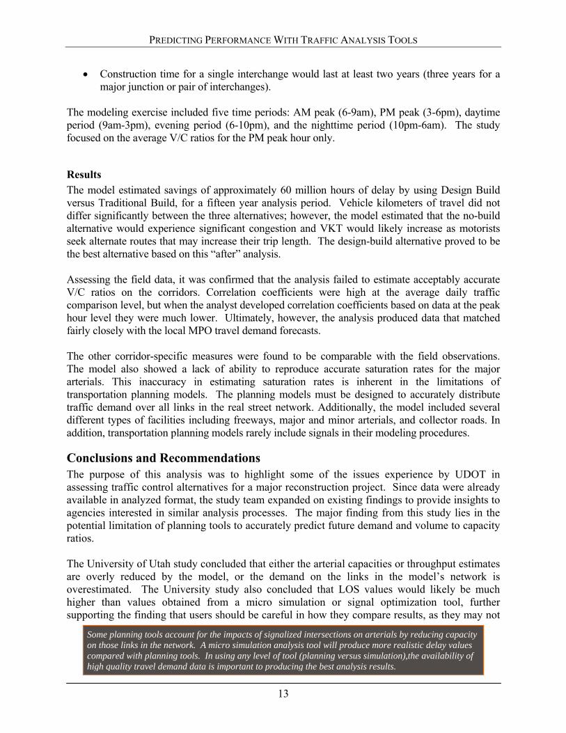
Figure 7: SR 826/Palmetto Expressway at NW 67th (Left) and NW 57th Avenue (Right)
The Florida DOT design team completed an Interchange Operational Analysis Report (IOAR) which was submitted to Department in December 2004 for the westbound (WB) off-ramps at the NW 67th and NW 57th Avenues interchanges. The report recommended construction of a continuous WB auxiliary lane, and widening of the off-ramps to two lanes, along with operational improvements to the intersections. The Scoping Committee requested a study of the recently improved eastbound off ramps, at NW 67th and 57th Avenues, in order to verify whether the objectives of that project have been accomplished. The recommended improvements included widening of the off-ramps and adding a continuous auxiliary lane between both interchanges. Due to the similarities in configuration and recommendations, it was decided that an evaluation of before and after conditions in the EB direction (including actual and microsimulation comparisons) would be the best way to establish whether the proposed WB improvements in the IOAR (December 2004) are sound and worth pursuing.
Description The SR 826-Palmetto Expressway is a high-speed limited access facility with a posted speed of 55 mph. The mainline facility has a typical section consisting of six lanes divided from west of NW 67th Avenue to east of NW 57th Avenue. Travel lanes are approximately 12 feet wide with 7-foot inside shoulders and outside shoulders approximately 10 feet wide. A one-way frontage road (NW 167th Street) is located on the north and south sides of the mainline facility. The frontage road provides two lanes in each direction with a posted speed of 40 mph. Figure 8 illustrates the existing conditions geometry for both interchanges after the construction of the EB improvement project.
16

PREDICTING PERFORMANCE WITH TRAFFIC ANALYSIS TOOLS
Figure 8: Existing Conditions Geometry (EB Improvement Project Post-Construction)
Year 2004 (Post-Construction) Existing Traffic Volumes
For the purpose of this comparative analysis, the existing year (2004) A.M. and P.M. peak hour volumes were taken directly from the SR 826-Palmetto Expressway IOAR (December 2004), referenced above. The method used in the IOAR (December 2004) to develop the A.M. and P.M. peak hour volumes for the mainline, ramps and intersections is briefly described below. For additional details such as traffic flow patterns, origin-destination survey and historical crash data, refer to the IOAR (December 2004).
Mainline and Ramp Traffic Volumes
Year 2003 Average Annual Daily Traffic (AADT) volumes for SR 826-Palmetto Expressway mainline and ramps were obtained from the FDOT’s 2003 Florida Traffic Information CD. The 2003 mainline and ramp volumes were projected to year 2004 volumes by applying a growth factor of 0.5 percent. This applied growth factor was based on the historical records from the Department’s traffic counting stations. The growth rate was computed from a regression analysis using the Department’s Trends Analysis Spreadsheet. The A.M. and P.M. peak hour traffic volumes were estimated by applying appropriate K-factors to the AADT.
Intersection Traffic Volumes
Turning movement and seventy-two hour continuous traffic counts were collected at the signalized intersections for both A.M. (7:00 to 9:00 A.M.) and P.M. (4:00 to 6:00 P.M.) peak hours during typical weekdays in April 2004.
17
PREDICTING PERFORMANCE WITH TRAFFIC ANALYSIS TOOLS
Year 2000 (Pre-Construction) Traffic Volumes
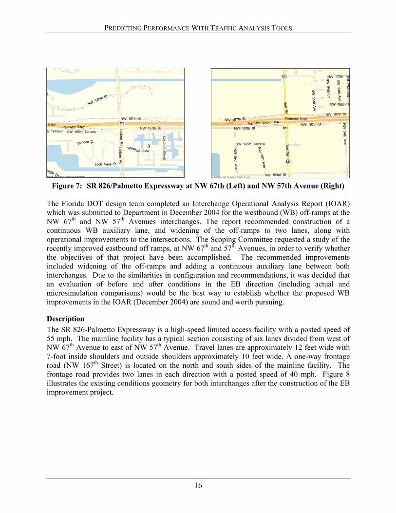
A comparison of historical AADTs from the 2004 Florida Department of Transportation Traffic Data CD was done based on key stations along the corridor. Table 2 provides a summary of this comparison. As shown in the table, the 2001 AADTs declined from the previous year AADTs, due to construction. For this reason, volumes for the year 2000 were determined to be representative of the most recent entire pre-construction year along the corridor. Also shown in Table 2 below, is the average reduction factor of 0.91 applied to the Year 2004 (Post-Construction) volumes taken from the IOAR (December 2004) to develop the Year 2000 (Pre-Construction) volumes. Table 2: Historical AADTs and Reduction Factor
Reduction FactorSite Description 2000 2001* 2004
'00 - '04 '01-'04
9060 SR 826 W NW 67 Ave 116000 111500 135467 0.856 0.823
0554 SR 826 W NW 57 Ave 123500 118500 116500 1.060 1.017
0405 SR 826 E NW 57 Ave 136000 134000 149000 0.913 0.899
0038 SR 823 (NW 57th Ave) N NW 159th St 52500 47000 59500 0.882 0.790
1190 SR 823 (NW 57th Ave) S NW 173rd Dr 54000 54500 63000 0.857 0.865
AVERAGE REDUCTION FACTOR 0.914 0.888
* Beginning of the construction year Figure 9 illustrates the Year 2000 (Pre-Construction) traffic volumes that were developed for the A.M. and P.M. peak hour periods for the mainline, ramps, and signalized intersections.
18

PREDICTING PERFORMANCE WITH TRAFFIC ANALYSIS TOOLS
Figure 9: Year 2000 (Pre-Construction) A.M. and P.M. Peak Hour Traffic Volumes
Analysis and Results
Ramps, Mainline and Intersection Level of Service Analysis Comparison
For the purpose of comparing the traffic conditions before and after construction at the eastbound off-ramps at NW 67th and NW 57th Avenue, the results of a micro-simulation model for SR 826 – Palmetto Expressway IOAR (December, 2004) for A.M. and P.M. peak hours were obtained by Florida DOT. The existing geometry was reviewed and assumed for the Year 2004 (Post-Construction) conditions. The geometry and traffic volumes were revised for the Year 2000 (Pre-Construction) conditions. Listed below are revisions made to the geometry.
NW 67th Avenue - reduced to one-lane eastbound off-ramp NW 57th Avenue – reduced to one-lane eastbound off-ramp Removal of eastbound auxiliary lane between NW 67th and NW 57th Avenues
Eastbound Ramp Merge / Diverge Level of Service Analysis Comparison
The eastbound off-ramps at the interchanges of NW 67th Avenue and NW 57th Avenue were improved from one-lane to two-lanes with a full auxiliary lane between the NW 67th Avenue interchange on-ramp and NW 57th Avenue interchange two-lane off-ramp. Ramps were analyzed utilizing the ramp module of the Highway Capacity Manual and other relevant methodology on ramps from the Highway Capacity Manual. The hourly volumes were converted to peak flow rates by applying truck factors, peak hour factors (PHF), driver population parameter, and
19

PREDICTING PERFORMANCE WITH TRAFFIC ANALYSIS TOOLS
passenger car equivalents as described in Highway Capacity Manual. Table 3 summarizes results of the ramps merge/diverge analyses. Table 3: Year 2000 (Pre-Construction) and Year 2004 (Post-Construction) Comparison Freeway Ramp Merge / Diverge Analysis Derived from the HCM
AM Peak Hour PM Peak Hour Interchange Location
Direction Number of Lanes Volume Ramp LOS Volume Ramp LOS
Year 2000 (Pre-Construction)
EB off 1 490 C 640 C SR 826 at NW 67th Avenue EB on 1 1,160 D 760 C
EB off 1 510 D 640 C SR 826 at NW 57th Avenue EB on 1 740 D 640 C
Year 2004 (Post-Construction)
EB off 2 540 B 700 B SR 826 at NW 67th Avenue EB on 1 1,270 B 830 B
EB off 2 560 B 700 B SR 826 at NW 57th Avenue EB on 1 810 D 700 C
As seen in Table 3 and in the Highway Capacity Manual methodology output, a comparison of pre and post construction conditions indicate improvements in the level of service, even when considering that the traffic in the segment has grown almost 10% between 2000 and 2004.
Mainline Level of Service
Levels of service analyses from the micro-simulation model and the Highway Capacity Manual software were conducted for the mainline for Year 2000 (Pre-Construction) and Year 2004 (Post-Construction). Tables 4 and 5 summarize the comparative results for A.M. and P.M. peak hour freeway mainline in the eastbound direction for pre-construction and post-construction conditions.
Micro-simulation Results
The A.M. peak hour results from the model do not indicate significant differences or marked improvements in the post construction condition, with the exception of west of the N.W. 67th Avenue off-ramp. The eastbound mainline segment between the NW 67th Avenue on-ramp and the NW 57th Avenue off-ramp indicated to be within the acceptable level of service standard for pre-construction at LOS C but for post-construction the level of service dropped below the standard level of service to LOS E. This is primarily due to the traffic increases that have occurred since the construction took place, which have caused congestion at the intersections and the mainline, congestion which then spills back into the ramps under study.
20

PREDICTING PERFORMANCE WITH TRAFFIC ANALYSIS TOOLS
Table 4: Year 2000 (Pre-Construction and Year 2004 (Post-Construction) Comparison A.M. and P.M. Peak Hour Freeway Mainline Micro-simulation Analysis Summary
A.M. Peak Hour
2000 (Pre-) 2004 (Post-) From To
Density LOS Density LOS
West of NW 67th Avenue NW 67th Avenue Off-Ramp 19.27 C 17.42 B
NW 67th Avenue Off-Ramp NW 67th Avenue On-Ramp 17.74 B 19.59 C
NW 67th Avenue On-Ramp NW 57th Avenue Off-Ramp 23.47 C 38.17 E
NW 57th Avenue Off-Ramp NW 57th Avenue On-Ramp 21.49 C 23.63 C
NW 57th Avenue On-Ramp East of 57th Avenue 23.72 C 26.66 D
P.M. Peak Hour
2000 (Pre-) 2004 (Post-) From To
Density LOS Density LOS
West of NW 67th Avenue NW 67th Avenue Off-Ramp 19.72 C 17.92 B
NW 67th Avenue Off-Ramp NW 67th Avenue On-Ramp 17.31 B 18.95 C
NW 67th Avenue On-Ramp NW 57th Avenue Off-Ramp 20.52 C 17.54 B
NW 57th Avenue Off-Ramp NW 57th Avenue On-Ramp 17.62 B 19.30 C
Highway Capacity Manual Software Results
Given the shortcomings of the microsimulation model, which produced spillbacks that did not allow the proper isolated evaluation of the auxiliary lane, the freeway module of the Highway Capacity Manual software was chosen as an alternative tool to better analyze and isolate conditions relevant to the auxiliary lane project. Table 5 provides the summary of the analysis. Based on the Highway Capacity Manual software freeway analysis, a comparison of ‘before and after’ conditions indicates generally unchanged levels of service and decreases in density along key sections of the mainline, even considering that the traffic in the section has grown almost 10% since the eastbound auxiliary lane was completed
21
PREDICTING PERFORMANCE WITH TRAFFIC ANALYSIS TOOLS
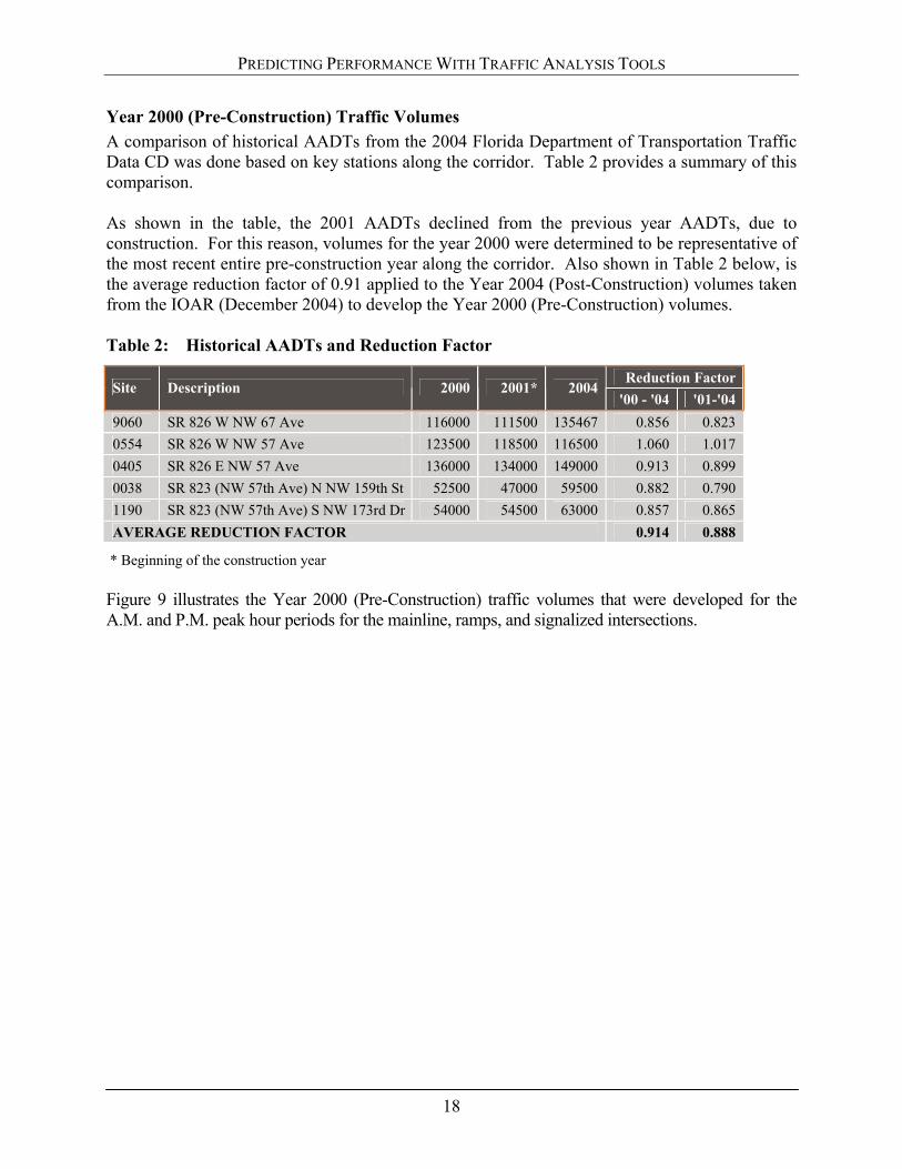
Table 5: Year 2000 (Pre-Construction and Year 2004 (Post-Construction) Comparison A.M. and P.M. Peak Hour Freeway Mainline HCM Analysis Summary
A.M. Peak Hour
2000 (Pre-) 2004 (Post-) From To
Density LOS Density LOS
West of NW 67th Avenue NW 67th Avenue Off-Ramp 21.90 C 18.00 C
NW 67th Avenue Off-Ramp NW 67th Avenue On-Ramp 18.90 C 20.80 C
NW 67th Avenue On-Ramp NW 57th Avenue Off-Ramp 25.90 C 21.30 C
NW 57th Avenue Off-Ramp NW 57th Avenue On-Ramp 22.80 C 25.00 C
NW 57th Avenue On-Ramp East of NW 57th Avenue 27.30 D 30.10 D
P.M. Peak Hour
2000 (Pre-) 2004 (Post-) From To
Density LOS Density LOS
West of NW 67th Avenue NW 67th Avenue Off-Ramp 22.20 C 18.30 C
NW 67th Avenue Off-Ramp NW 67th Avenue On-Ramp 18.30 C 20.10 C
NW 67th Avenue On-Ramp NW 57th Avenue Off-Ramp 22.90 C 18.90 C
NW 57th Avenue Off-Ramp NW 57th Avenue On-Ramp 19.10 C 21.00 C
NW 57th Avenue On-Ramp East of NW 57th Avenue 22.90 C 25.20 C
Conclusions and Recommendations The purpose of this analysis was to evaluate how much the construction of the expanded freeway eastbound ramps and auxiliary lanes contributed to improving the freeway’s operations. As expected the microsimulation model accurately represented the existing freeway operations and properly forecasted spillbacks from downstream. By replicating the spillbacks, however, the analysis of the auxiliary lanes as an isolated improvement was not possible to distinguish. Under these circumstances the HCM software was applied in order to evaluate the auxiliary lane as an isolated improvement in order to determine the benefits of the improvement. The HCM comparative analysis indicated that the eastbound improvements yielded moderate improvements in the freeway and ramp operations. Therefore a recommendation was made to construct similar improvements in the westbound direction.
Extensions and Guidance
Level of Effort
Case Study 3’s geographic scope is relatively limited to several interchanges and the supporting frontage roads and arterial system feeding into the interchange areas. Due to the limited roadway system that was under study, the required amount of time to input the network and traffic data for the microsimulation model was modest. If the study area was wider in scope then the setup time would be significantly higher. For the deterministic HCM model, the setup time was minimal. HCM models are relatively simplistic in their data and network requirements and require minimal labor for their application.
22

PREDICTING PERFORMANCE WITH TRAFFIC ANALYSIS TOOLS
Traffic Analysis Software Selection
An aspect of any traffic analysis study is the selection of the proper software package that best meets the objectives of the study. In Case Study 3, the objective of the project was to identify how well individual roadway improvements improved the freeway traffic operations. Many times as was the case in the Palmetto Interchange Analysis, spillback traffic as shown in the microsimulation model masked the operational improvements of the expanded ramps and auxiliary lane. By using the deterministic HCM model, the spot improvements due to the expanded ramps could be evaluated without being masked by the system deficiencies. An important lesson from Case Study 3 is for traffic engineers to select the best package that will fulfill the specific objectives of the study. When evaluating specific spot improvements such as individual ramps or limited merge areas simpler traffic analysis tools such as the HCM models may be more appropriate and effective than microsimulation models.
Modeling Process
An important lesson to learn in this case study is that microsimulation models can be used and be quite useful for conducting before and after studies even though a formal before study was not completed prior to the construction of a transportation improvement.
Data Development
Typical applications of traffic analysis software require existing as well as future traffic such as traffic volumes and turning movements. In this case study rather than forecasting the future, the model was used to recreate the traffic operational conditions prior to the completion of the improved ramps and auxiliary lanes. Traffic data for the Year 2000 prior to the construction project was developed based on traffic reduction factors established by mainline freeway historical counts. The case study demonstrated that through the development of traffic reduction factors sufficient traffic information can be developed for practical application to microsimulation models.
Measure of Effectiveness Issue
In the conduct of this study two separate software packages were applied; microsimulation and a deterministic HCM model procedure. Each program has their unique procedures for determining the level of service and measure of effectiveness. As demonstrated in this study, if the HCM procedure of Level of Service definition as used in the deterministic HCM model will be the standard, then the microsimulation results must be converted into an equivalent measure of effectiveness as defined in the HCM. For this case study all microsimulation results were converted into density and the equivalent Level of Service to match the results of the HCM procedure. Whenever a microsimulation model is used it is imperative that an HCM equivalence be established as was done in this study when using HCM Levels of Service.
Special thanks to Florida Department of Transportation District 6 and the Consulting Team for providing details and insights for use in these comparisons.
23
PREDICTING PERFORMANCE WITH TRAFFIC ANALYSIS TOOLS
CASE STUDY 4: I-25 AND UNIVERSITY BOULEVARD IN DENVER, COLORADO. Converting a Cloverleaf Interchange to a Single-Point Urban Interchange
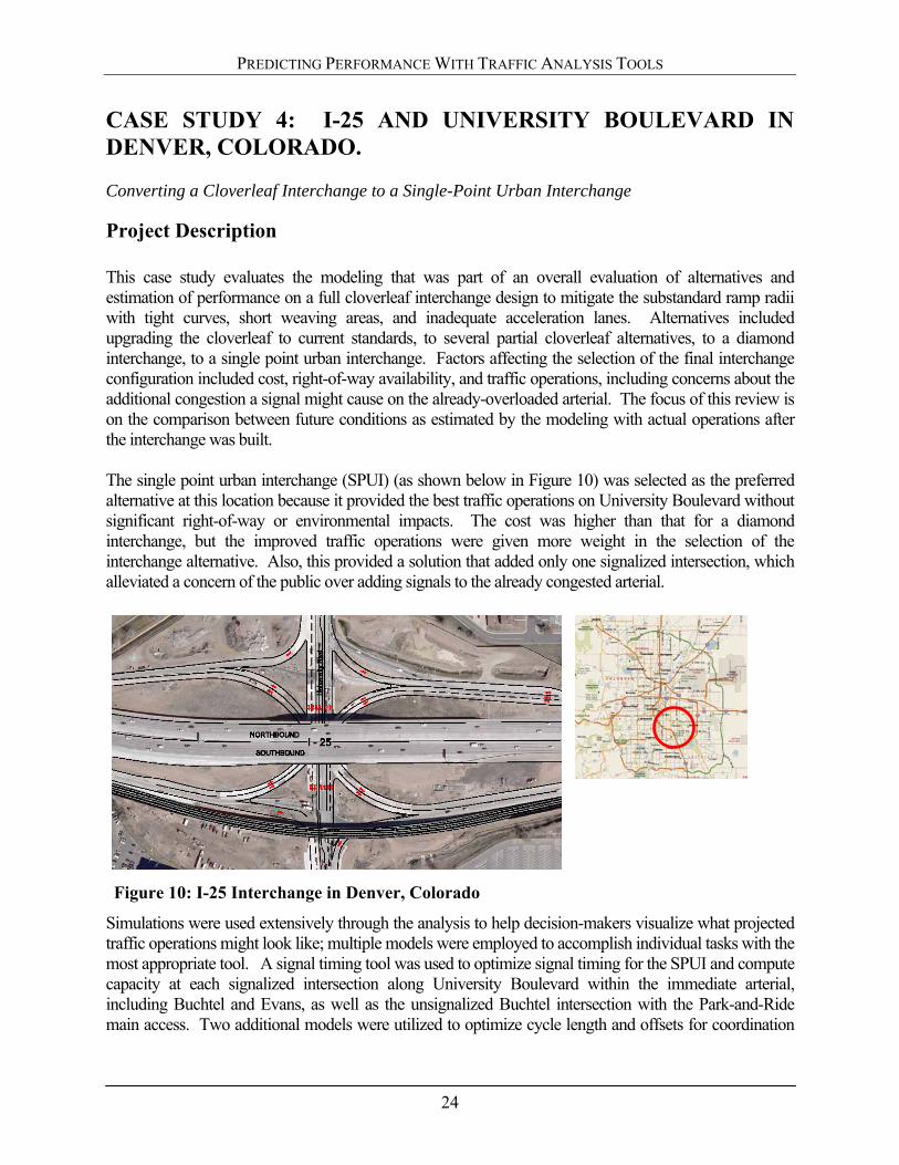
Project Description This case study evaluates the modeling that was part of an overall evaluation of alternatives and estimation of performance on a full cloverleaf interchange design to mitigate the substandard ramp radii with tight curves, short weaving areas, and inadequate acceleration lanes. Alternatives included upgrading the cloverleaf to current standards, to several partial cloverleaf alternatives, to a diamond interchange, to a single point urban interchange. Factors affecting the selection of the final interchange configuration included cost, right-of-way availability, and traffic operations, including concerns about the additional congestion a signal might cause on the already-overloaded arterial. The focus of this review is on the comparison between future conditions as estimated by the modeling with actual operations after the interchange was built. The single point urban interchange (SPUI) (as shown below in Figure 10) was selected as the preferred alternative at this location because it provided the best traffic operations on University Boulevard without significant right-of-way or environmental impacts. The cost was higher than that for a diamond interchange, but the improved traffic operations were given more weight in the selection of the interchange alternative. Also, this provided a solution that added only one signalized intersection, which alleviated a concern of the public over adding signals to the already congested arterial.
Simulations were used extensively through the analysis to help decision-makers visualize what projected traffic operations might look like; multiple models were employed to accomplish individual tasks with the most appropriate tool. A signal timing tool was used to optimize signal timing for the SPUI and compute capacity at each signalized intersection along University Boulevard within the immediate arterial, including Buchtel and Evans, as well as the unsignalized Buchtel intersection with the Park-and-Ride main access. Two additional models were utilized to optimize cycle length and offsets for coordination
Figure 10: I-25 Interchange in Denver, Colorado
24

PREDICTING PERFORMANCE WITH TRAFFIC ANALYSIS TOOLS
through the corridor. Finally, a separate simulation tool was used throughout for delay and Level of Service (LOS) estimates for consistency in comparing alternatives.
Conditions Prior to Construction
The University Boulevard Interchange with I-25 was a typical cloverleaf configuration, with direct ramps serving each of the eight movements in the interchange. University Boulevard was two lanes per direction with 12-ft lanes in the interchange area. I-25 was three lanes per direction through the interchange.
The interchange had a number of deficiencies, including the northbound I-25 to northbound University ramp with poor sight distance caused by substandard geometric conditions with no acceleration lane at University Boulevard where 12-ft lanes were being narrowed to 11-ft lanes; the southbound I-25 to southbound University ramp with poor sight distance caused by substandard geometric conditions with the ramp terminus within several hundred feet of the intersection of University Boulevard and Buchtel Boulevard where queuing created stop-and-go conditions; and, the weaving areas on I-25 experienced congestion associated with the short weaving distance through a vertical crest which limited sight distance.
There were also several capacity deficiencies related to the interchange, including the
northbound weave on I-25 operated at LOS F during both peak hours; the southbound weave on I-25 operated at LOS E during both peak hours; and the weave between the southern ramp termini and the Buchtel Boulevard intersection operated poorly during both peak periods due to the short weaving distances.
SPUI Selected
The SPUI and diamond interchanges provide the following safety benefits:
The northbound I-25 to northbound University exit ramp moves south, allowing for an improved design with a better acceleration lane and sight distance.
The southbound I-25 to southbound University ramp moves away from the Buchtel Boulevard intersection, allowing for a lengthened weaving section.
The signal(s) meter southbound University Boulevard traffic for larger weaving gaps. The northbound University to southbound I-25 ramp moves away from Buchtel Boulevard,
increasing the weaving distance. The weaving sections on I-25 are eliminated.
The SPUI was selected as operationally superior to the diamond interchange, with better mid-block operations and better interchange LOS. The SPUI provides the additional benefits of adding only one signal to University Boulevard and increasing signal spacing between the interchange and Buchtel. This information is intended to provide background on the ultimate project, but our focus will be on the SPUI as built.
25

PREDICTING PERFORMANCE WITH TRAFFIC ANALYSIS TOOLS
Operations Analysis
For the purposes of this review, opening day estimates were the focus in order to compare model predictions with actual operations. The build scenario volumes were distributed to the SPUI. The following traffic analyses were conducted:
Optimized individual intersection timings; Optimized corridor for coordinated operations; and Simulated the interchange area using the optimized signal timing.
Delay values were extracted from simulation to determine levels of service (LOS) for the various alternatives for both AM and PM peak periods. The effects of a park-and-ride lot on Buchtel just off University were made part of the analysis for projected use of the LRT station there. Levels of service were obtained for signalized locations using a capacity analysis tool as shown in Table 6. It should be noted here that while earlier in the original study, when analyzing individual signalized intersections, HCM procedures were used, the use of LOS is not entirely appropriate in this table given that the delays were generated from simulation.
Table 6: Simulation-Generated Delay and Levels of Service AM PM
Opening Day Delay LOS Delay LOS
SPUI
Northbound 47 D 50 D
Westbound 41 D 41 D
Southbound 25 C 25 C
Eastbound 31 C 31 C
Buchtel
Northbound 187 F 208 F
Westbound 41 D 44 D
Southbound 12 B 13 B
Eastbound 169 F 190 F
Evans
Northbound 85 F 83 F
Westbound 301 F 309 F
Southbound 294 F 302 F
Eastbound 69 E 73 E
26
PREDICTING PERFORMANCE WITH TRAFFIC ANALYSIS TOOLS
Analysis and Results Some issues that are apparent when reviewing this particular study raise several questions:
A. Did the use of multiple tools and the ways they were integrated and compared help or hinder the accuracy and comprehensive coverage of the results?
B. Was data collected using conventional stop-bar turning movement counts that show departure flow rates instead of measuring demand by quantifying arrival rates?
C. Were oversaturated conditions properly modeled incorporating the unmet demand into delay computations in multiple-period analyses?
D. Were the effects of the downstream signalized intersections at Buchtel and Evans properly considered, including spillback during peak periods?
E. Was the use of simulation instead of HCM methods to ascertain LOS for the various components appropriate?
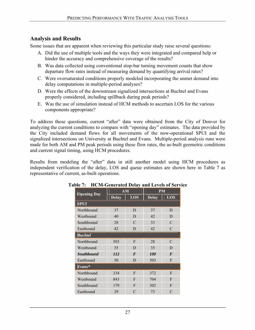
To address these questions, current “after” data were obtained from the City of Denver for analyzing the current conditions to compare with “opening day” estimates. The data provided by the City included demand flows for all movements of the now-operational SPUI and the signalized intersections on University at Buchtel and Evans. Multiple-period analysis runs were made for both AM and PM peak periods using these flow rates, the as-built geometric conditions and current signal timing, using HCM procedures. Results from modeling the “after” data in still another model using HCM procedures as independent verification of the delay, LOS and queue estimates are shown here in Table 7 as representative of current, as-built operations.
Table 7: HCM-Generated Delay and Levels of Service AM PM
Opening Day Delay LOS Delay LOS
SPUI
Northbound 37 D 37 D
Westbound 40 D 42 D
Southbound 28 C 33 C
Eastbound 42 D 42 C
Buchtel
Northbound 503 F 28 C
Westbound 35 D 35 D
Southbound 112 F 100 F
Eastbound 50 D 503 F
Evans*
Northbound 334 F 372 F
Westbound 843 F 704 F
Southbound 179 F 302 F
Eastbound 29 C 73 C
27

PREDICTING PERFORMANCE WITH TRAFFIC ANALYSIS TOOLS
When compared with the original study predictions shown in Table 7, the major discrepancy is the estimate of delay and LOS for the southbound approach at Buchtel (with the northbound approach at Evans another inconsistency). The study predicted LOS B, but the current conditions are clearly LOS F. This is most likely due to the spillback from Evans, which could have been foreseen from its LOS predictions. (One other discrepancy was the PM estimate for the NB approach at Buchtel, which is created because the current capacity analysis did not account for the spillover from the short left-turn bay there.)
Conclusions and Recommendations After comparing the original case study results with our current analysis, each question raised in the Analysis of Results is addressed below.
A. The original study effectively used multiple analysis tools to take advantage of the strengths of each. One tool was used to quantify capacity and LOS at each intersection, including the SPUI, as well as signal timing for that intersection. Another tool was utilized to determine signal coordination and to confirm delay and LOS for the signals operating as a corridor. Finally, another tool was used to simulate the operations of the corridor to obtain delay estimates consistent within one model. This worked out to be an effective use of multiple tools for this application.
B. Although it is not clear from the original report, existing count data did not seem to include unmet demands judging from the delay and LOS results yielding such good operations. This may have shown a better than reality situation for the current conditions, but did not have a negative effect on the alternative selection process and of course was not a factor in the future condition analysis.
C. Projection estimates were not constrained by actual counts and did appear to properly consider the appropriate demand levels for the future operating situations. Therefore, the analyses using these projections did model oversaturated conditions showing some extreme delay levels in some cases as proved to be the case after reviewing the “after” conditions.
D. Multiple models showed the excessive queue estimates and predicted the spillback from the Buchtel and Evans signalized intersections to be an issue. While these tools quantified the magnitude of these queues, some were not effective in modeling the effects of the bottleneck on adjacent intersections. The scope of the original study and this review was limited to the southbound approaches to Buchtel and Evans as potentially affecting the SPUI. The southbound flow rates simply seem to overwhelm the available capacity in all analyses, to the point additional lane capacity would be needed to mitigate.
E. The use of simulation overcame the shortcomings of standard capacity analysis procedures for these spillback situations. The results did accurately predict the bottlenecks, particularly at Evans, spilling back through Buchtel and affecting the SPUI, which actual “after” counts confirm.
The quote from the initial study shows that this was recognized in the analysis: “However, [the spillback] had only a minor effect on the new southbound I-25 to southbound University Boulevard ramp, and no effect on the SPUI intersection. The minor queuing on the southbound I-25 to southbound University Boulevard ramp due to the southbound University Boulevard
28

PREDICTING PERFORMANCE WITH TRAFFIC ANALYSIS TOOLS
queuing did not affect freeway operations because this ramp is fed by the proposed collector/distributor roadway, and not directly by the interstate.” The failure along this corridor was accurately predicted and acknowledged in the study, with agreement that the collector-distributor ramp length would prevent freeway problems.
Extensions and Guidance In summary, results show that the new interchange is operating well when considered individually, and this is confirmed in discussions with City engineering staff. However, the oversaturated conditions at the downstream signals create a spillback situation for the SB I-25 to SB University movement; impeding the flow from this off-ramp and backing it up during peak hours. A contributing factor is the pedestrian demand at Buchtel from the University of Denver activity, which forces timing to be more limited for vehicles traveling SB on University than would be used for vehicular traffic only. A more comprehensive analysis would have extended to recommend improvements to the Buchtel and Evans signalized intersections, especially Evans since it is apparent the southbound bottleneck originates here. Alternative analyses at the Evans signal could have provided mitigating improvement choices to resolve the congestion along the corridor. The conclusion in the study that these queues did not significantly affect the subject of the study (the SPUI) were based on the fact that the southbound exit ramp was extremely long and has enough storage to prevent backing up to the freeway. While this is true and actual current operations bear this out, it does not address the still existing congestion along the corridor and even on this ramp. Solving the problem at Evans would have indeed prevented the poor operations for this important leg of the SPUI, thereby improving the level of service at the subject of the study. There could have been multiple-period HCM analyses performed at the Evans signal to at least generate future improvements to address the source of the only real problem found at the SPUI. As for Buchtel, investigating strategies to overcome the interference by the large numbers of pedestrians accessing the University of Denver could have been explored. Closing two crosswalks and/or double cycling the pedestrian call to maximize the vehicular efficiency might have been worth modeling to more effectively use the green time for vehicular traffic. Another, more costly but still worth a look, could have been a pedestrian overpass, including approaching the University for possibly sharing in its expense. While these signalized intersections were modeled, the results showing the bottleneck could have been used to further investigate alternatives to resolve the problem. A broader look at the corridor might have prevented the problem that still exists today.
Special thanks to Paul Brown from the Colorado DOT’s consulting team for information on the case study, and to Amy Rens and Paul Bountry of the City of Denver for providing detailed “after” data for use in these comparisons.
29
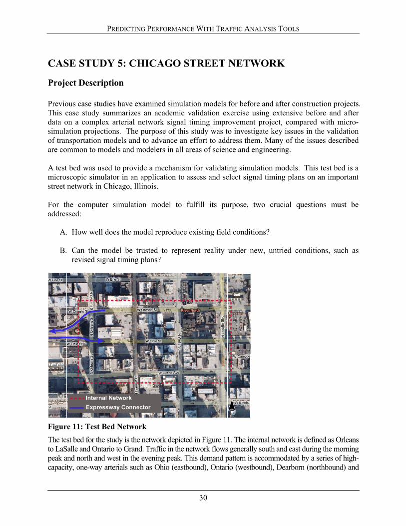
PREDICTING PERFORMANCE WITH TRAFFIC ANALYSIS TOOLS
CASE STUDY 5: CHICAGO STREET NETWORK
Project Description Previous case studies have examined simulation models for before and after construction projects. This case study summarizes an academic validation exercise using extensive before and after data on a complex arterial network signal timing improvement project, compared with micro-simulation projections. The purpose of this study was to investigate key issues in the validation of transportation models and to advance an effort to address them. Many of the issues described are common to models and modelers in all areas of science and engineering. A test bed was used to provide a mechanism for validating simulation models. This test bed is a microscopic simulator in an application to assess and select signal timing plans on an important street network in Chicago, Illinois. For the computer simulation model to fulfill its purpose, two crucial questions must be addressed:
A. How well does the model reproduce existing field conditions? B. Can the model be trusted to represent reality under new, untried conditions, such as
revised signal timing plans?
Internal NetworkExpressway Connector
Figure 11: Test Bed Network
The test bed for the study is the network depicted in Figure 11. The internal network is defined as Orleans to LaSalle and Ontario to Grand. Traffic in the network flows generally south and east during the morning peak and north and west in the evening peak. This demand pattern is accommodated by a series of high-capacity, one-way arterials such as Ohio (eastbound), Ontario (westbound), Dearborn (northbound) and
30

PREDICTING PERFORMANCE WITH TRAFFIC ANALYSIS TOOLS
Clark and Wells (southbound), in addition to LaSalle (northbound and southbound). Traffic generally flows south and east in the morning and north and west in the evening through this signalized intersection network. The question being addressed was to quantify how well simulation, with proper calibration, reproduces the patterns as experienced in reality.
Characteristics and Inputs
Microscopic simulation represents single vehicles entering the road network at random times moving second-by-second according to local interaction rules such as car-following logic, lane changing, response to traffic control devices, and turning at intersections according to prescribed probabilities. The network has 112 1-way links, 30 signalized intersections, and about 38,000 vehicles moving through it per hour. Streets are modeled as directed links with intersections as nodes. There are a variety of inputs or specifications that must be made, either directly or by default values provided. Signal settings are direct inputs and were singled out as controllable factors since altering these inputs to produce improved traffic flow drives the study. For validation, the signal plan will be the one in the field. For finding optimal fixed-time signal-timing plans, the signal parameters will necessarily be manipulated.
Data Collection
Initial field data for the network were collected on a single day, 7 am to 10 am and 3 pm to 6 pm with the analyses limited to the three one-hour periods, 8 am to 9 am, 4 pm to 5 pm, and 5 pm to 6 pm. This covered the peak periods and a “shoulder” period. Traffic volume data were collected manually and by video recording. There were very few pedestrians, and they had no discernible effect on traffic. Incidents were not included, but because illegal parking was an endemic condition, the network was coded to account for its effect. Free-flow speed was selected on the basis of posted speed limits. Signal timing plans and bus routes were collected directly in the field.
Analysis and Results The interest in the model here is its value in assessing and producing good time-of-day signal plans. Comparisons between the field and model results were made through selected evaluation functions to deal with the issues raised.
Evaluation Functions
Stop time (stopped delay) was chosen on approaches to intersections as the primary evaluation function as the typical measure by which intersection level of service (LOS) is evaluated. Other criteria such as throughput, delay, travel time, and queue length are all highly correlated with stop time. Drivers on urban street networks are particularly sensitive to stop time, spurring traffic managers to seek its reduction. In fact, the Highway Capacity Manual’s (HCM) selection of stopped delay for LOS designation is meant to reflect the user’s perception of the intersection’s quality of service. The quantities for STV (stop time per vehicle) or STVS (stop time for vehicle stopped) for aggregations of approaches (routes or corridors) are very difficult to obtain, requiring the
31

PREDICTING PERFORMANCE WITH TRAFFIC ANALYSIS TOOLS
tracking of individual vehicles. By summing over the individual links, a “pseudo stop time” is created for the corridor. This will be close to a real stop time, provided vehicles turning off of or onto the corridor exhibit no difference from those traveling through.
Calibration
Calibration is adjusting input parameters to match model output. Two types of calibration were done in the test bed example. The first addressed the blockage of turns at two intersections and the subsequent gridlock. The network was altered to facilitate the bypass of the blockage without affecting throughput. The second was necessary because of a substantial difference on one link (at the LaSalle/Ontario intersection) between the field and the model stop times. This difference was largely resolved by changing the free flow speed from 30 miles per hour (mph) to 20 mph to be consistent with the observed (from video) speed of vehicles as opposed to the speed limit.
Throughput Comparison
A net change in internal total throughput indicates discrepancies showing less output in the morning and more output in the evening. This is due to the garage effect: vehicles disappear to the parking lots in the morning and reappear from them in the evening; since the morning and evening runs do not span the entire day, there are invariably differences in the counts. The means of 100 replicated model runs are close to the observed counts.
Stop Time Comparisons
The distribution of stop time at each approach shows definite discrepancies at some locations. Examination of video and model animation exposes the key cause: the model does not fully reflect driver behavior. Lane utilization in the model is not consistent with lane utilization in the field. Vehicles joining long queues where they are briefly stopped may not appear in the simulation as having stopped. This accounts for smaller STVS in the field than in the model. The STVS is larger in the model because it counts only vehicles that completely stopped, so the average time per stop is higher However, the key measure of how long truly stopped vehicles are delayed appears to match what is seen in the field quite reasonably.
Prediction and Validation
A new signal timing plan was put in place in September. Under these new circumstances, predictions were to be made and data collection designed for a day in September expected to be similar to the date of the first data collection in May. The model was run with the May input,
except for the updated signal timing. After the data were collected in September, the
results were compared on several key links. This showed that throughput and stop time performance (STVS) were reasonably close. However, when the effect of change in demand was checked, it was noted that the model has difficulty dealing with storage of vehicles on short, congested links just downstream of a wide intersection.
Table 8: ▲ Model Compared with ▲ Field
Link ▲ Model ▲ Reality
SB Ohio at LaSalle 0 3
SB LaSalle at Ohio -11 -10
NB LaSalle at Ontario -9 -5
NB Orleans to Freeway 13 15
NB Orleans at Ontario 1 -2
32
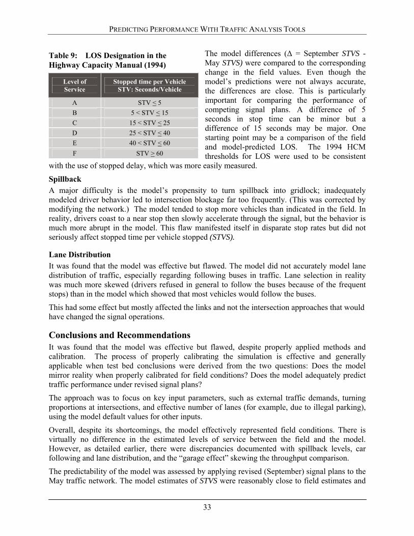
PREDICTING PERFORMANCE WITH TRAFFIC ANALYSIS TOOLS
The model differences (Δ = September STVS - May STVS) were compared to the corresponding change in the field values. Even though the model’s predictions were not always accurate, the differences are close. This is particularly important for comparing the performance of competing signal plans. A difference of 5 seconds in stop time can be minor but a difference of 15 seconds may be major. One starting point may be a comparison of the field and model-predicted LOS. The 1994 HCM thresholds for LOS were used to be consistent
with the use of stopped delay, which was more easily measured.
Table 9: LOS Designation in the Highway Capacity Manual (1994)
Level of Service
Stopped time per Vehicle STV: Seconds/Vehicle
A STV < 5
B 5 < STV < 15 C 15 < STV < 25 D 25 < STV < 40 E 40 < STV < 60 F STV > 60
Spillback
A major difficulty is the model’s propensity to turn spillback into gridlock; inadequately modeled driver behavior led to intersection blockage far too frequently. (This was corrected by modifying the network.) The model tended to stop more vehicles than indicated in the field. In reality, drivers coast to a near stop then slowly accelerate through the signal, but the behavior is much more abrupt in the model. This flaw manifested itself in disparate stop rates but did not seriously affect stopped time per vehicle stopped (STVS).
Lane Distribution
It was found that the model was effective but flawed. The model did not accurately model lane distribution of traffic, especially regarding following buses in traffic. Lane selection in reality was much more skewed (drivers refused in general to follow the buses because of the frequent stops) than in the model which showed that most vehicles would follow the buses.
This had some effect but mostly affected the links and not the intersection approaches that would have changed the signal operations.
Conclusions and Recommendations It was found that the model was effective but flawed, despite properly applied methods and calibration. The process of properly calibrating the simulation is effective and generally applicable when test bed conclusions were derived from the two questions: Does the model mirror reality when properly calibrated for field conditions? Does the model adequately predict traffic performance under revised signal plans?
The approach was to focus on key input parameters, such as external traffic demands, turning proportions at intersections, and effective number of lanes (for example, due to illegal parking), using the model default values for other inputs.
Overall, despite its shortcomings, the model effectively represented field conditions. There is virtually no difference in the estimated levels of service between the field and the model. However, as detailed earlier, there were discrepancies documented with spillback levels, car following and lane distribution, and the “garage effect” skewing the throughput comparison.
The predictability of the model was assessed by applying revised (September) signal plans to the May traffic network. The model estimates of STVS were reasonably close to field estimates and
33

PREDICTING PERFORMANCE WITH TRAFFIC ANALYSIS TOOLS
the model LOSs were, for the most part, similar to those observed in the field. More importantly, the model successfully tracks changes in traffic performance over time: on five links for which field data were available, two links exhibited a reduction in STVS, one link an increase, and two had no significant change; the model’s predictions were the same.
In summary, a candid assessment of the model is that with careful calibration and tuning, the model output will match field observations and be an effective predictor of operational performance.
Extensions and Guidance This case study is an excellent example illustrating some potential limitations of simulation and the importance of calibration and validation for practitioners. In this analysis, there were particular shortcomings of the model exposed when comparing its simulation with reality. Some could be overcome with adjustments to the parameters within the model and some were accepted as normal variations.
This points to the need for calibration guidance for users in order to minimize the limitations or flaws in any simulation tool. There were particular steps taken in this study to overcome specific discrepancies. More general guidance could be offered to users to assist their calibration procedures.
Users of simulation models need to fine-tune all inputs that are related to the driving behavior and vehicle characteristics by comparing and adjusting some absolute measures. This procedure for calibration and validation should include:
1 SIMULATION MODEL SETUP
Determination of Measure of Effectiveness
Field Data Collection
Network Coding
2 INITIAL EVALUATION
Default Parameter Set
Multiple Run
6 PARAMETER CALIBRATION
Genetic Algorithm
Multiple Run
7 EVALUATION OF PARAMETER SET
Statistical Test
Visualization Check
8 MODEL VALIDATION
Multiple Run
FEEDBACK
3 INITIAL CALIBRATION
Identification of Calibration Parameters
Experimental Design
Multiple Run
4 FEASIBILITY TEST
X-Y Plots
Statistical Test
Identification of KeyParameters
5 ADJUSTMENT
Adjustment of KeyParameters
Comparing the results from the model with actual field conditions;
Assessing the applicability of the initial set of parameters, defaults and assumptions;
Defining acceptable ranges for all parameters for the given analysis characteristics;
Scrutinizing the results from multiple runs to compare model results with field data;
Viewing animation against known field operations for any unrealistic conditions;
Figure 12: Evaluation Steps
Validating new data by comparing results with new field conditions The flow chart shown in Figure 12 is from “Microscopic Simulation Model Calibration and Validation Handbook October 2006,” Byungkyu (Brian) Park and Jongsun Won. This is an
34
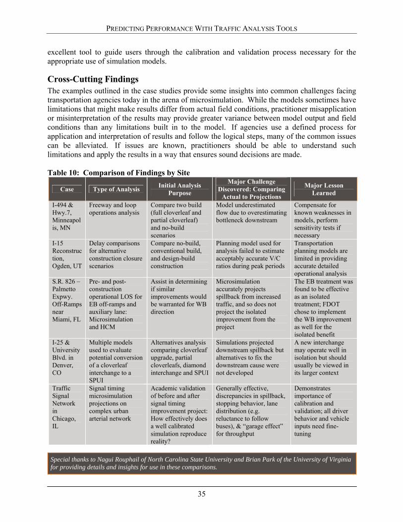
PREDICTING PERFORMANCE WITH TRAFFIC ANALYSIS TOOLS
excellent tool to guide users through the calibration and validation process necessary for the appropriate use of simulation models.
Cross-Cutting Findings The examples outlined in the case studies provide some insights into common challenges facing transportation agencies today in the arena of microsimulation. While the models sometimes have limitations that might make results differ from actual field conditions, practitioner misapplication or misinterpretation of the results may provide greater variance between model output and field conditions than any limitations built in to the model. If agencies use a defined process for application and interpretation of results and follow the logical steps, many of the common issues can be alleviated. If issues are known, practitioners should be able to understand such limitations and apply the results in a way that ensures sound decisions are made. Table 10: Comparison of Findings by Site
Case Type of Analysis Initial Analysis
Purpose
Major Challenge Discovered: Comparing
Actual to Projections
Major Lesson Learned
I-494 & Hwy.7, Minneapolis, MN
Freeway and loop operations analysis
Compare two build (full cloverleaf and partial cloverleaf) and no-build scenarios
Model underestimated flow due to overestimating bottleneck downstream
Compensate for known weaknesses in models, perform sensitivity tests if necessary
I-15 Reconstruction, Ogden, UT
Delay comparisons for alternative construction closure scenarios
Compare no-build, conventional build, and design-build construction
Planning model used for analysis failed to estimate acceptably accurate V/C ratios during peak periods
Transportation planning models are limited in providing accurate detailed operational analysis
S.R. 826 – Palmetto Expwy. Off-Ramps near Miami, FL
Pre- and post- construction operational LOS for EB off-ramps and auxiliary lane: Microsimulation and HCM
Assist in determining if similar improvements would be warranted for WB direction
Microsimulation accurately projects spillback from increased traffic, and so does not project the isolated improvement from the project
The EB treatment was found to be effective as an isolated treatment; FDOT chose to implement the WB improvement as well for the isolated benefit
I-25 & University Blvd. in Denver, CO
Multiple models used to evaluate potential conversion of a cloverleaf interchange to a SPUI
Alternatives analysis comparing cloverleaf upgrade, partial cloverleafs, diamond interchange and SPUI
Simulations projected downstream spillback but alternatives to fix the downstream cause were not developed
A new interchange may operate well in isolation but should usually be viewed in its larger context
Traffic Signal Network in Chicago, IL
Signal timing microsimulation projections on complex urban arterial network
Academic validation of before and after signal timing improvement project: How effectively does a well calibrated simulation reproduce reality?
Generally effective, discrepancies in spillback, stopping behavior, lane distribution (e.g. reluctance to follow buses), & “garage effect” for throughput
Demonstrates importance of calibration and validation; all driver behavior and vehicle inputs need fine-tuning
Special thanks to Nagui Rouphail of North Carolina State University and Brian Park of the University of Virginia for providing details and insights for use in these comparisons.
35

PREDICTING PERFORMANCE WITH TRAFFIC ANALYSIS TOOLS
Freeway widening projects, such as the one in Minnesota, can often shift a bottleneck downstream to another location. Bottlenecks in the roadway system can significantly affect operating conditions. Modeling can help determine the needed expanse for the widening project to avoid major impacts from a bottleneck shifted downstream. Modelers should be aware that level of service guidelines were designed for use with the Highway Capacity Manual procedures. Metrics such as density and delay that are derived from a microsimulation tool do not provide for direct comparison with such HCM thresholds since they were produced using different procedures. Field measured metrics can be directly compared with HCM LOS thresholds. Insights into the magnitude and duration of poor operating conditions are important. Often, temporal descriptions of results are needed to help decision makers understand operations. For example, LOS F should be accompanied by the time period over which it occurs, how long it lasts, and if an improvement reduces the metric in question but does not change level of service overall. Microsimulation projects can require large amounts of data and information. Modelers should build in realistic timeframes that are based on anticipated project-by-project requirements for data collection, processing, and information gathering. Transportation agency processes often make use of microsimulation models to help determine a particular course of action. More than one “build” alternative may be considered along with the “no build” alternative. Less frequently, microsimulation models are used to predict future performance of the maintenance of traffic alternatives. Expanded use of these tools to predict future construction zone operating conditions can help agencies design a Maintenance of Traffic Plan and help minimize impacts from during construction, as shown in the Utah Case Study. Microsimulation is not necessarily needed for every potential idea for a project. Agencies should prioritize and identify, based on appropriate information and data, the top alternatives to focus on. Modeling can be useful in supporting investment decisions. The modeling exercise is typically consistent with the scale of the overall project investment. Tools are available to assist practitioners at the micro, meso, and macro levels (ordered in decreasing levels of detail). For example, a macro level analysis tool is useful in determining future demand for a facility, while a micro level tool allows for additional detail in quantifying impacts at the individual vehicle level. Appropriate timelines and levels of detail should be matched with the appropriate tool. As shown in the Palmetto Expressway Interchange Case Study, microsimulation can aggregate impacts from multiple improvements. Modelers should determine whether or not they need to understand the benefits and impacts from each individual improvement prior to developing the model. If so, it may be useful to investigate other tools to gain insights into the direct performance of individual improvements. The Denver Case Study was also a good example of how to make use of multiple tools in order to take advantage of the strengths of each.
36

PREDICTING PERFORMANCE WITH TRAFFIC ANALYSIS TOOLS
Prior to model development, data collection plans should be designed to account for unmet demand. Automatic traffic detection equipment typically does not account for demand caused by queuing, but occupancy levels and other measures can be used to determine whether or not saturated conditions may exist. As shown to potentially have occurred in the Denver Case Study, lack of information on unmet demand can significantly affect modeling results. Queuing is normally adequately accounted for and the effects can be understood using microsimulation. As illustrated in the Denver Case Study, the Highway Capacity Manual procedure is limited in that it does not include the effects of queue spillback at an intersection approach. As shown in the Chicago Case Study, it is important to properly calibrate a simulation model to ensure adequate impacts from queuing are reported and included in the analysis of alternatives.
37

PREDICTING PERFORMANCE WITH TRAFFIC ANALYSIS TOOLS
PRACTICAL GUIDANCE ON THE APPLICATION OF TRAFFIC SIMULATION AND ANALYSIS TOOLS FOR TRANSPORTATION-INVESTMENT DECISIONS The remainder of this document provides insights into some common issues in the application of microsimulation tools. These issues are followed by specific actions that can be taken within a defined modeling process to either alleviate the issue or to allow practitioners to make decisions with a solid understanding of the potential impacts of the issue. These ideas were supported based on findings from interviews with local practitioners at each case study location.
Issues and Pitfalls of Implementation (So Why Didn’t My Analysis Work?) The most important concept for a user to remember is that software modeling tools are nothing more than mathematical equations that are attempting to replicate human behavior. Deterministic models try to simulate actions of aggregated drivers and micro-simulation models try to replicate individual driver movements. In either case aggregate behavior or individual behavior will vary due to a wide degree of variables including but not limited to age, driver experience, geographic area, time of day, weather conditions, congestion, and trip purpose. It requires an experienced traffic engineer and software model user to avoid the many pitfalls that will result in a traffic analysis not replicating existing or future driver behavior. Based on the case studies, interviews with dozens of traffic engineers, and the authors’ personal experiences, the most common pitfalls to avoid for a successful application of traffic operational software are as follows:
A. Overuse of Default Values (Or It’s in the Model – It Has to Be Right) – The practice of using software packages without verifying the default values is very common. The tendency is for users to simply to apply the default values because of the high cost and limited project budgets to verify the values.
The odds of taking a software package out of its shrink wrap and successfully replicating existing ground conditions are very remote. Many software packages are developed outside of the United States. The software developers will use default values that are suitable for drivers of their particular countries. For example, many of the roundabout software packages overestimate the capacity by 20% when applied to US conditions (reference NCHRP Report 572 for Project 3-65, “Roundabouts in the United States”). One reason for this overestimation may be the values used in the packages are based on international drivers who are more familiar with the operations of a roundabout and this is reflected in their default values for variables such as critical gap time.
The type and range of default values may be extensive. Values such as critical gap times, follow up times, car following and lane changing algorithms, saturation flows, pedestrian walking speeds, lost time, and design vehicle characteristics such as acceleration and deceleration rates are just a few of the variables a user of traffic
38
PREDICTING PERFORMANCE WITH TRAFFIC ANALYSIS TOOLS
operations software packages needs to consider.
So What Should a User Do?
Before using a software package, it is critical for the user to determine and review the default values that are contained within the package. The review should also look at the mathematical equations which are included as the model algorithms. For example, in the Highway Capacity Manual as part of the procedure for determining the impact of parking on intersection capacity, the equation assumes it takes 18 seconds to park a car. For determining the impact of buses on the system it assumes that the buses are stopping for 14.4 seconds. The user must determine if these values are reasonable for their analysis. This determination should be done before the model is applied as part of a project analysis.
But there are so many default values! And how do you determine what the values should be? In the end, it is the experience of the user that is absolutely critical when establishing what reasonable values are. And that experience must be applied on a project by project basis. However, experience must be supported by verification, and that leads to Overcoming Pitfall B …
B. Calibration (Or Trust the Model But Verify) – Many interviewees indicated that
calibrating the traffic operations model is absolutely critical. As indicated in Issue A using the default values from the software packages means that the models will most likely not simulate field conditions. All models from microsimulation to deterministic must be calibrated in order to simulate correctly.
For example, in a recent environmental study conducted in Washington, DC, as part of an operational analysis the levels of service for an unsignalized intersection were determined. The HCM based model predicted that the intersection would experience delays of up to 300 seconds on the minor road. Yet when a field check was conducted, the typical minor street delays were in the range of 30 seconds. A thorough review of the analysis indicated that the volume counts were correct and all data had been inputted correctly. So the team looked at the default values used in the model and tried to verify them in the field. As a result, it was determined that the typical critical gap times of the drivers at the intersection were 1 to 1.5 seconds lower than the gap times used in the model. Lower critical gap times mean higher capacity and less delays experienced by the drivers. As a result the critical gap times were lowered and the model replicated the 30 seconds of typical delay experienced by drivers at the unsignalized intersection.
So What Should a User Do?
Models that are being applied in a region or study area for the first time should be calibrated. If the study is for a future site, the model should be applied to nearby existing intersections or roadway sections and the user should verify that it can replicate existing traffic operations.
39

PREDICTING PERFORMANCE WITH TRAFFIC ANALYSIS TOOLS
The real question is how we select the variable or variables that should be modified so that the model may be calibrated. Again the answer lies in having an experienced traffic engineer who is familiar with the software and the sensitivity of the model variables to conduct the calibration effort. Even with an experienced user, the calibration of the model may require a significant level of effort.
C. Queuing Analysis (Or How Far Back Will That Queue Go?) – During the
interviews several users recognized that queue analysis was absolutely critical for determining the operational characteristics of the intersection or roadway. In fact several interviewees indicated that they were more concerned with the models accurately predicting the queues than the level of service.
In at least one of the case studies the major breakdown in the analysis was not accurately predicting the backup conditions downstream from the project. The existing analysis and the improvement simply moved the problem downstream and the backup interfered with the project's operation.
So What Should a User Do?
The first step the user should take is to validate and calibrate the model(s) as discussed in Pitfall (?) B. If the model variables have been reviewed and the model is still not simulating the queues accurately it very well may be that the area coverage is not large enough. The system analysis must cover the entire affected area. In some cases the project boundaries are too small and do not include areas which may influence the model results. For example, a major improvement beyond the project study area may affect the traffic volume or cause traffic to divert. The application of the model in the limited project area may not recognize the potential change in traffic patterns.
D. Unusual Geometrics and Conditions (Or This Is Above and Beyond the Call of
Duty) – Many of the models are limited in their capability of analyzing unusual geometric or traffic conditions. Examples are 3 lane or 5 lane sections, rail lines through intersections, heavy pedestrian movements, complex signal controls, five or six legged intersections, oversaturated conditions, etc. So What Should a User Do? The various software packages all have strengths and weaknesses and different capabilities for analyzing unusual geometrics and conditions. The first step a user must take is to match the software’s capabilities with the given conditions to be analyzed. Sometimes field conditions are so complex that one software package cannot meet the analytical requirements for a study involving complex field conditions. Under these conditions, a combination of software packages might be considered. For
40
PREDICTING PERFORMANCE WITH TRAFFIC ANALYSIS TOOLS
example, in a recent corridor study in Vermont, the project involved a series of signalized intersections, arterial sections, roundabouts, unsignalized intersections, freeway ramps, multilane facilities, rail operations in the corridor, and a need for demonstrating operations to the public through animation. No one software package has the capability of meeting all the analysis requirements and therefore a combination of four different packages were selected for the analysis.
E. Inaccurate Field Data (Or What Was That Field Crew Doing Out There?) –
Sometimes the models are not inaccurate, but the analysis is conducted with poor field data. The model user must always consider if the field data they have is accurate. Was the data collected on a typical day? Was there a breakdown of the counting equipment? Was there human error? The user must always remember that traffic varies from day to day, which means there will always be some variation between the model simulation and typical traffic conditions. How the data is collected could also affect the results. For example, at intersections field crews often count traffic by recording the number of vehicles entering the intersection - a reasonable technique as long as you do not have saturated conditions. However, only counting the vehicles that go through the intersection means by definition the analysis should never show volume exceeding capacity. If saturated conditions exist and you do not count the queued vehicles, the models will never replicate field conditions. So What Should a User Do? When conducting a traffic operations analysis not only should you look at the model parameters but a thorough analysis of how the data input was collected should be considered. Again, the most important element of an accurate project analysis are the users’ experience and their ability to know what makes sense and what does not when reviewing field data.
F. Inaccurate Travel Demand Forecasting (Or the Forecast Is Right, We Just Got the Wrong Year) – The travel demand models have built-in inaccuracies which are passed on to the traffic operations software that uses their traffic volume forecasts as part of future year operations analysis. The demand models many times are in error due to land use changes or population and employment forecasts that are simply wrong.
So What Should a User Do? When developing design year traffic, it is a good practice not to use raw traffic assignments from the traffic demand models. Rather develop growth factors based simulating existing and future traffic assignments. The growth factors should then be used to expand existing ground counts. The result is a much more accurate future traffic forecast and a more accurate operational analysis.
41
PREDICTING PERFORMANCE WITH TRAFFIC ANALYSIS TOOLS
G. Inaccurate Origin-Destination Information (Or Tell Me Where They Are Coming From and Where They Are Going) – More advanced microsimulation models typically require the user to not only input traffic counts but also where these vehicles are coming from and where are they going. The microsimulation models use the origin/destination information to route the traffic through the system. Improvements in the transportation network may result in the model rerouting the traffic as part of its analysis. However, the original origins and destinations for the traffic entering into the system will not change. Most software packages have the origins and destinations as inputs that do not vary and do not analyze potential future changes even if within the project there are significant travel time improvements that may change the traffic patterns. This insensitivity to forecast changes in the origins and destinations may result in significant errors.
So What Should a User Do? Microsimulation software is constantly being updated. The next generation of microsimulation software very well may be interconnected to regionwide travel demand models. The next generation of traffic software will allow the user to incorporate an iteration process where the results of an operational analysis will be reiterated back through the regional travel demand models. However, until the software development catches up to the demand analysis requirements, for analysis of major regionwide transportation improvements the analysts could manually reiterate the results back through the regional travel demand forecasting model and rerun the microsimulation traffic operations software. A reiteration model application should be used only with a great deal of caution because it is only necessary for the largest regional transportation improvements. For smaller size improvements once is enough and the iteration process will make only an insignificant improvement in the results.
H. Sanity Checks (Or It Must Be Right It Comes From a Computer) – There is a tendency to over-rely on the results of the traffic operations models. Sanity checks should be made by the experienced user to determine if the results make sense. Too many times the user believes the model is working because it produces numbers.
So What Should a User Do? Sometimes a user cannot see the forest because of the trees. A simple but effective way to conduct a sanity check is to get a second opinion. Look at the final results and if the model says we are handling 3000 vehicles per hour per lane and they are moving at 60 miles an hour it’s time to get a new model. Look at the results and see if the traffic forecast is physically possible.
I. Demand Data (Or Do You Know How to Count Traffic?) – Most turning
movement counts at signalized intersections are performed by counting vehicles as the pass through the intersection and ignoring the unmet demand. This produces
42

PREDICTING PERFORMANCE WITH TRAFFIC ANALYSIS TOOLS
43
unrealistic data in oversaturated conditions that do not represent the true demand at the intersection. Performing capacity analyses using data collected this way can severely underestimate the delay and back-of-queue results and yield inaccurate levels of service. For congested signals, arrival demand (not departure flows) must be used for the capacity analysis to accurately match field conditions.
So What Should a User Do?
Counting the unmet demand at the end of each period for adding to the departure flows yields the more appropriate arrival demands that should be used in these analyses. This can be done by estimating the length of the queue at the beginning of the red phase at the end of each period for all movements. These distances can be converted into vehicles per lane and added to the through volumes to produce arrival demand for each period. It is important to proportion the queued vehicles at the same turning rates as the through count for that period, and to count the unmet demand only once (subtracting it from the subsequent through count). For signalized intersection capacity analyses, congested conditions require multiple-period analyses using the unmet demand for each period as the initial queue for the subsequent period to accurately compute the third delay term (d3).
J. Different Definitions of Level of Service (Or I Can't Define the LOS F But I
Know It When I See It) – Different software packages have different definitions of level of service. Although the Highway Capacity Manual defines the measures of effectiveness for various levels of service most traffic operations software packages use their own definitions of level of service. For example, when analyzing levels of service for roundabouts, some packages use the level of service criteria for signalized intersections versus unsignalized intersections. Some microsimulation packages may not even calculate density and have no direct correlation to the HCM level of service So What Should a User Do When first using a software package, the user must review what and how the package is developing levels of service. The review should look at how the software is treating different types of facilities such as freeways, ramps, weaving areas, multilanes, signalized intersections, and unsignalized intersections. If the definitions of levels of service are different than the HCM definition then an equivalency should be established. Sometimes this is established by using the microsimulation to optimize the highway operations and then reanalyzing the facility by using an HCM based software package. The user should also be careful when relying simply on a visual display of a software package to get a sense of what the level of service may be. It is critical for the user to review the evaluation output files rather than rely on the visual display to get a true understanding of the facility’s level of service operations.

Office of OperationsRoom E86-205
1200 New Jersey Avenue, SEWashington, DC 20590
www.ops.fhwa.dot.gov
FHWA-HOP-08-055