Traditional IR models Jian-Yun Nie

1

Main IR processes Last lecture: Indexing – determine the

important content terms

Next process: Retrieval ◦ How should a retrieval process be done? Implementation issues: using index (e.g. merge of lists) (*) What are the criteria to be used?

◦ Ranking criteria What features? How should they be combined? What model to use? 2

Cases one-term query:

The documents to be retrieved are those that include the term

- Retrieve the inverted list for the term - Sort in decreasing order of the weight of the word

Multi-term query? - Combining several lists - How to interpret the weight? - How to interpret the representation with all the

indexing terms for a document? (IR model)

3

What is an IR model? Define a way to represent the contents of a

document and a query Define a way to compare a document

representation to a query representation, so as to result in a document ranking (score function)

E.g. Given a set of weighted terms for a document ◦ Should these terms be considered as forming a

Boolean expression? a vector? … ◦ What do the weights mean? a probability, a feature

value, … ◦ What is the associated ranking function?

4

Plan

This lecture ◦ Boolean model ◦ Extended Boolean models ◦ Vector space model ◦ Probabilistic models Binary Independent Probabilistic model Regression models

Next week ◦ Statistical language models

5

Early IR model – Coordinate matching score (1960s) Matching score model ◦ Document D = a set of weighted terms ◦ Query Q = a set of non-weighted terms

Discussion ◦ Simplistic representation of documents and

queries ◦ The ranking score strongly depends on the term

weighting in the document If the weights are not normalized, then there will be

great variations in R

6

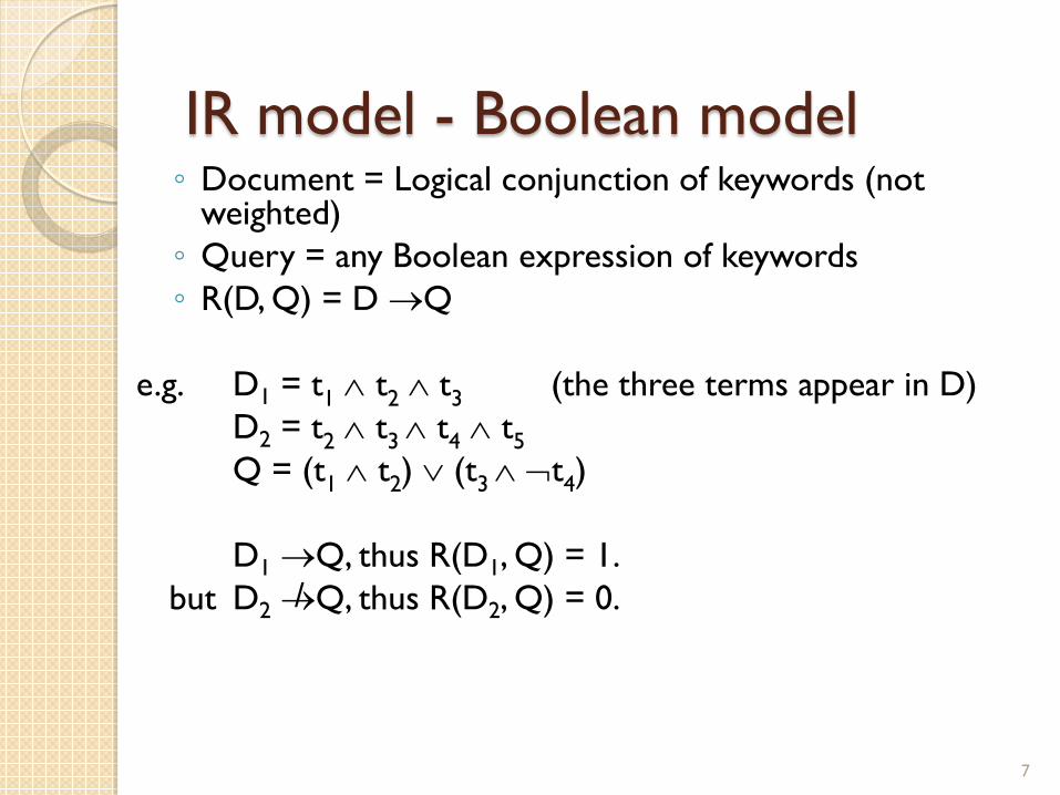
IR model - Boolean model ◦ Document = Logical conjunction of keywords (not

weighted) ◦ Query = any Boolean expression of keywords ◦ R(D, Q) = D →Q

e.g. D1 = t1 ∧ t2 ∧ t3 (the three terms appear in D) D2 = t2 ∧ t3 ∧ t4 ∧ t5 Q = (t1 ∧ t2) ∨ (t3 ∧ ¬t4) D1 →Q, thus R(D1, Q) = 1. but D2 →Q, thus R(D2, Q) = 0.

7

/

Properties

Desirable ◦ R(D,Q∧Q)=R(D,Q∨Q)=R(D,Q) ◦ R(D,D)=1 ◦ R(D,Q∨¬Q)=1 ◦ R(D,Q∧¬Q)=0

Undesirable ◦ R(D,Q)=0 or 1

8

Boolean model Strengths ◦ Rich expressions for queries ◦ Clear logical interpretation (well studied logical properties) Each term is considered as a logical proposition The ranking function is determine by the validity of a logical

implication

Problems: ◦ R is either 1 or 0 (unordered set of documents) many documents or few/no documents in the result No term weighting in document and query is used

◦ Difficulty for end-users for form a correct Boolean query E.g. documents about kangaroos and koalas kangaroo ∧ koala ? kangaroo ∨ koala ? Specialized application (Westlaw in legal area)

Current status in Web search ◦ Use Boolean model (ANDed terms in query) for a first

step retrieval ◦ Assumption: There are many documents containing all the

query terms find a few of them 9

Extensions to Boolean model (for document ranking)

D = {…, (ti, wi), …}: weighted terms Interpretation: ◦ Each term or a logical expression defines a fuzzy set ◦ (ti, wi): D is a member of class ti to degree wi. ◦ In terms of fuzzy sets, membership function: µti(D)=wi

A possible Evaluation: R(D, ti) = µti(D) ∈ [0,1]

R(D, Q1 ∧ Q2) = µQ1∧Q2 (D) = min(R(D, Q1), R(D, Q2)); R(D, Q1 ∨ Q2) = µQ1( Q2 (D) = max(R(D, Q1), R(D, Q2)); R(D, ¬Q1) = µ¬Q1 (D) = 1 - R(D, Q1).

10

Recall on fuzzy sets Classical set ◦ a belongs to a set S: a∈S, ◦ or no: a∉S

Fuzzy set ◦ a belongs to a set S to some degree

(μS(a)∈[0,1]) ◦ E.g. someone is tall

0

0,5

1

1,5

1,5 1,7 1,9 2,1 2,3

μtall(a)

11

Recall on fuzzy sets

Combination of concepts

0

0,2

0,4

0,6

0,8

1

1,2

Allan Bret Chris Dan

TallStrongTall&Strong

12

Extension with fuzzy sets Can take into account term weights Fuzzy sets are motivated by fuzzy concepts in

natural language (tall, strong, intelligent, fast, slow, …)

Evaluation reasonable? ◦ min and max are determined by one of the elements

(the value of another element in some range does not have a direct impact on the final value) - counterintuitive ◦ Violated logical properties μA∨¬A(.)≠1 μA∧¬A(.)≠0

13

Alternative evaluation in fuzzy sets

R(D, ti) = µti(D) ∈ [0,1]

R(D, Q1 ∧ Q2) = R(D, Q1) * R(D, Q2);

R(D, Q1 ∨ Q2) = R(D, Q1) + R(D, Q2) - R(D, Q1) * R(D, Q2);

R(D, ¬Q1) = 1 - R(D, Q1).

◦ The resulting value is closely related to both values ◦ Logical properties μA∨¬A(.)≠1 μA∧¬A(.)≠0 μA∨A(.)≠μA(.) μA∧A(.)≠μA(.)

◦ In practice, better than min-max ◦ Both extensions have lower IR effectiveness than

vector space model

14

IR model - Vector space model Assumption: Each term corresponds to a

dimension in a vector space Vector space = all the keywords encountered <t1, t2, t3, …, tn> Document D = < a1, a2, a3, …, an> ai = weight of ti in D Query Q = < b1, b2, b3, …, bn> bi = weight of ti in Q R(D,Q) = Sim(D,Q)

15

Matrix representation

t1 t2 t3 … tn

D1 a11 a12 a13 … a1n

D2 a21 a22 a23 … a2n

D3 a31 a32 a33 … a3n … Dm am1 am2 am3 … amn

Q b1 b2 b3 … bn

16

Term vector space

Document space

Some formulas for Sim

Dot product Cosine Dice Jaccard

17

∑ ∑ ∑∑

∑ ∑∑

∑ ∑

∑∑

−+=

+=

=

=•=

i i iiiii

iii

i iii

iii

i iii

iii

iii

baba

baQDSim

ba

baQDSim

ba

baQDSim

baQDQDSim

) * (

) * (),(

) * (2),(

*

) * (),(

) * (),(

22

22

22

t 1

D

Q

t 3

t 2

θ

Document-document, document-query and term-term similarity t1 t2 t3 … tn

D1 a11 a12 a13 … a1n

D2 a21 a22 a23 … a2n

D3 a31 a32 a33 … a3n … Dm am1 am2 am3 … amn

Q b1 b2 b3 … bn

D-D similarity

D-Q similarity

t-t similarity

18

Euclidean distance

When the vectors are normalized (length of 1), the ranking is the same as cosine similarity. (Why?)

( )∑ =−=−

n

i kijikj dddd1

2,,

19

Implementation (space) Matrix is very sparse: a few 100s terms for a document,

and a few terms for a query, while the term space is large (>100k)

Stored as: D1 → {(t1, a1), (t2,a2), …} t1 → {(D1,a1), …} (recall possible compressions: ϒ code)

20

Implementation (time) The implementation of VSM with dot product: ◦ Naïve implementation: Compare Q with each D ◦ O(m*n): m doc. & n terms ◦ Implementation using inverted file:

Given a query = {(t1,b1), (t2,b2), (t3,b3)}: 1. find the sets of related documents through inverted file for each

term

2. calculate the score of the documents to each weighted query term (t1,b1) → {(D1,a1*b1), …} 3. combine the sets and sum the weights (∑)

◦ O(|t|*|Q|*log(|Q|)): |t|<<m (|t|=avg. length of inverted lists), |Q|*log|Q|<<n (|Q|=length of the query)

21

Pre-normalization

Cosine:

- use and to normalize the

weights after indexing of document and query - Dot product (Similar operations do not apply to Dice and

Jaccard)

∑∑

∑∑ ∑

∑==

jj

i

i

jj

i

j jii

iii

b

b

a

a

ba

baQDSim

2222 *

) * (),(

22

Best p candidates Can still be too expensive to calculate similarities to all

the documents (Web search) p best Preprocess: Pre-compute, for each term, its p nearest

docs. ◦ (Treat each term as a 1-term query.) ◦ lots of preprocessing. ◦ Result: “preferred list” for each term.

Search: ◦ For a |Q|-term query, take the union of their |Q| preferred

lists – call this set S, where |S| ≤ p|Q|. ◦ Compute cosines from the query to only the docs in S, and

choose the top k. ◦ If too few results, search in extended index

Need to pick p>k to work well empirically.

23

Discussions on vector space model Pros: ◦ Mathematical foundation = geometry Q: How to interpret?

◦ Similarity can be used on different elements

◦ Terms can be weighted according to their importance (in both D and Q)

◦ Good effectiveness in IR tests

Cons ◦ Users cannot specify relationships between terms world cup: may find documents on world or on cup only A strong term may dominate in retrieval

◦ Term independence assumption (in all classical models)

24

Comparison with other models ◦ Coordinate matching score – a special case ◦ Boolean model and vector space model: two extreme cases

according to the difference we see between AND and OR (Gerard Salton, Edward A. Fox, and Harry Wu. 1983. Extended Boolean information retrieval. Commun. ACM 26, 11, 1983) ◦ Probabilistic model: can be viewed as a vector space model

with probabilistic weighting.

25

Probabilistic relevance feedback If user has told us some relevant and some

irrelevant documents, then we can proceed to build a probabilistic classifier, such as a Naive Bayes model: ◦ P(tk|R) = |Drk| / |Dr| ◦ P(tk|NR) = |Dnrk| / |Dnr| tk is a term; Dr is the set of known relevant

documents; Drk is the subset that contain tk; Dnr is the set of known irrelevant documents; Dnrk is the subset that contain tk.

26

Why probabilities in IR?

User Information Need

Documents Document

Representation

Query Representation

How to match?

In traditional IR systems, matching between each document and query is attempted in a semantically imprecise space of index terms.

Probabilities provide a principled foundation for uncertain reasoning. Can we use probabilities to quantify our uncertainties?

Uncertain guess of whether document has relevant content

Understanding of user need is uncertain

27

Probabilistic IR topics

Classical probabilistic retrieval model ◦ Probability ranking principle, etc.

(Naïve) Bayesian Text Categorization/classification Bayesian networks for text retrieval Language model approach to IR ◦ An important emphasis in recent work

Probabilistic methods are one of the oldest but also one of the currently hottest topics in IR. ◦ Traditionally: neat ideas, but they’ve never won on

performance. It may be different now.

28

The document ranking problem We have a collection of documents User issues a query A list of documents needs to be returned Ranking method is core of an IR system: ◦ In what order do we present documents to the

user? ◦ We want the “best” document to be first, second

best second, etc…. Idea: Rank by probability of relevance of

the document w.r.t. information need ◦ P(relevant|documenti, query)

29

Recall a few probability basics

For events a and b: Bayes’ Rule

Odds:

∑ =

==

===∩=

aaxxpxbp

apabpbp

apabpbap

apabpbpbapapabpbpbapbapbap

,)()|(

)()|()(

)()|()|(

)()|()()|()()|()()|()(),(

)(1)(

)()()(

apap

apapaO

−==

Posterior

Prior

30

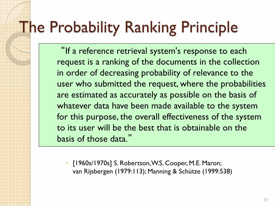
The Probability Ranking Principle “If a reference retrieval system's response to each

request is a ranking of the documents in the collection in order of decreasing probability of relevance to the user who submitted the request, where the probabilities are estimated as accurately as possible on the basis of whatever data have been made available to the system for this purpose, the overall effectiveness of the system to its user will be the best that is obtainable on the basis of those data.”

[1960s/1970s] S. Robertson, W.S. Cooper, M.E. Maron;

van Rijsbergen (1979:113); Manning & Schütze (1999:538)

31

Probability Ranking Principle

Let x be a document in the collection. Let R represent relevance of a document w.r.t. given (fixed) query and let NR represent non-relevance.

)()()|()|(

)()()|()|(

xpNRpNRxpxNRp

xpRpRxpxRp

=

=

p(x|R), p(x|NR) - probability that if a relevant (non-relevant) document is retrieved, it is x.

Need to find p(R|x) - probability that a document x is relevant.

p(R),p(NR) - prior probability of retrieving a (non) relevant document

1)|()|( =+ xNRpxRp

R={0,1} vs. NR/R

32

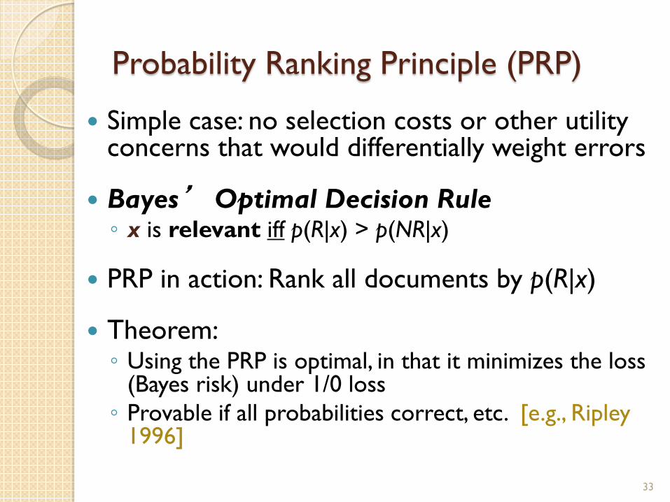
Probability Ranking Principle (PRP)

Simple case: no selection costs or other utility concerns that would differentially weight errors

Bayes’ Optimal Decision Rule ◦ x is relevant iff p(R|x) > p(NR|x)

PRP in action: Rank all documents by p(R|x)

Theorem: ◦ Using the PRP is optimal, in that it minimizes the loss

(Bayes risk) under 1/0 loss ◦ Provable if all probabilities correct, etc. [e.g., Ripley

1996]

33

Probability Ranking Principle

More complex case: retrieval costs. ◦ Let d be a document ◦ C - cost of retrieval of relevant document ◦ C’ - cost of retrieval of non-relevant document

Probability Ranking Principle: if for all d’ not yet retrieved, then d is the next

document to be retrieved We won’t further consider loss/utility from

now on

))|(1()|())|(1()|( dRpCdRpCdRpCdRpC ′−⋅′+′⋅≤−⋅′+⋅

34

Probability Ranking Principle

How do we compute all those probabilities? ◦ Do not know exact probabilities, have to use

estimates ◦ Binary Independence Retrieval (BIR) – which we

discuss later today – is the simplest model Questionable assumptions ◦ "Relevance" of each document is independent of

relevance of other documents. Really, it’s bad to keep on returning duplicates ◦ Boolean model of relevance (relevant or irrelevant) ◦ That one has a single step information need Seeing a range of results might let user refine query

35

Probabilistic Retrieval Strategy

Estimate how terms contribute to relevance ◦ How do things like tf, df, and length influence

your judgments about document relevance? One answer is the Okapi formulae (S. Robertson)

Combine to find document relevance

probability Order documents by decreasing probability

36

Probabilistic Ranking

Basic concept:

"For a given query, if we know some documents that are relevant, terms that occur in those documents should be given greater weighting in searching for other relevant documents.

By making assumptions about the distribution of terms and applying Bayes Theorem, it is possible to derive weights theoretically."

Van Rijsbergen

37

Binary Independence Model Traditionally used in conjunction with PRP “Binary” = Boolean: documents are represented as

binary incidence vectors of terms:

◦ ◦ iff term i is present in document x.

“Independence”: terms occur in documents independently

Different documents can be modeled as same vector

Bernoulli Naive Bayes model (cf. text categorization!)

),,( 1 nxxx =

1=ix

38

Binary Independence Model Queries: binary term incidence vectors Given query q, ◦ for each document d need to compute p(R|q,d). ◦ replace with computing p(R|q,x) where x is binary

term incidence vector representing d Interested only in ranking

Will use odds and Bayes’ Rule:

)|(),|()|(

)|(),|()|(

),|(),|(),|(

qxpqNRxpqNRp

qxpqRxpqRp

xqNRpxqRpxqRO

==

39

Binary Independence Model

• Using Independence Assumption:

∏=

=n

i i

i

qNRxpqRxp

qNRxpqRxp

1 ),|(),|(

),|(),|(

),|(),|(

)|()|(

),|(),|(),|(

qNRxpqRxp

qNRpqRp

xqNRpxqRpxqRO

⋅==

Constant for a given query Needs estimation

• So :

40

Binary Independence Model

∏=

⋅=n

i i

i

qNRxpqRxpqROdqRO

1 ),|(),|()|(),|(

• Since xi is either 0 or 1:

∏∏== =

=⋅

==

⋅=01 ),|0(

),|0(),|1(

),|1()|(),|(ii x i

i

x i

i

qNRxpqRxp

qNRxpqRxpqROdqRO

• Let );,|1( qRxpp ii == );,|1( qNRxpr ii ==

• Assume, for all terms not occurring in the query (qi=0) ii rp =

Then... This can be changed (e.g., in relevance feedback)

41

All matching terms Non-matching query terms

Binary Independence Model

All matching terms All query terms

∏∏

∏∏

===

====

−−

⋅−−

⋅=

−−

⋅⋅=

11

101

11

)1()1()|(

11)|(),|(

iii

iiii

q i

i

qx ii

ii

qx i

i

qx i

i

rp

prrpqRO

rp

rpqROxqRO

xi=1 qi=1

42

Binary Independence Model

Constant for each query

Only quantity to be estimated for rankings

∏∏=== −

−⋅

−−

⋅=11 11

)1()1()|(),|(

iii q i

i

qx ii

ii

rp

prrpqROxqRO

• Retrieval Status Value:

∑∏==== −

−=

−−

=11 )1(

)1(log)1()1(log

iiii qx ii

ii

qx ii

ii

prrp

prrpRSV

43

Binary Independence Model

• All boils down to computing RSV.

∑∏==== −

−=

−−

=11 )1(

)1(log)1()1(log

iiii qx ii

ii

qx ii

ii

prrp

prrpRSV

∑==

=1

;ii qx

icRSV)1()1(log

ii

iii pr

rpc−−

=

So, how do we compute ci’s from our data ?

44

Binary Independence Model • Estimating RSV coefficients. • For each term i look at this table of document counts:

Sspi ≈ )(

)(SNsnri −

−≈

)()()(log),,,(

sSnNsnsSssSnNKci +−−−

−=≈

• Estimates:

Sparck- Jones- Robertson formula 45

Estimation – key challenge

If non-relevant documents are approximated by the whole collection, then ri (prob. of occurrence in non-relevant documents for query) is n/N and ◦ log (1– ri)/ri = log (N– n)/n ≈ log N/n = IDF!

pi (probability of occurrence in relevant documents) can be estimated in various ways: ◦ from relevant documents if know some Relevance weighting can be used in feedback loop

◦ constant (Croft and Harper combination match) – then just get idf weighting of terms ◦ proportional to prob. of occurrence in collection more accurately, to log of this (Greiff, SIGIR 1998)

46

47

Iteratively estimating pi

1. Assume that pi constant over all xi in query ◦ pi = 0.5 (even odds) for any given doc

2. Determine guess of relevant document set: ◦ V is fixed size set of highest ranked documents

on this model (note: now a bit like tf.idf!) 3. We need to improve our guesses for pi and

ri, so ◦ Use distribution of xi in docs in V. Let Vi be set

of documents containing xi pi = |Vi| / |V|

◦ Assume if not retrieved then not relevant ri = (ni – |Vi|) / (N – |V|)

4. Go to 2. until converges then return ranking

Probabilistic Relevance Feedback 1. Guess a preliminary probabilistic

description of R and use it to retrieve a first set of documents V, as above.

2. Interact with the user to refine the description: learn some definite members of R and NR

3. Reestimate pi and ri on the basis of these ◦ Or can combine new information with original

guess (use Bayesian prior):

4. Repeat, thus generating a succession of approximations to R.

κκ++

=||

|| )1()2(

VpVp ii

iκ is prior

weight

48

PRP and BIR

Getting reasonable approximations of probabilities is possible.

Requires restrictive assumptions: ◦ term independence ◦ terms not in query don’t affect the outcome ◦ Boolean representation of

documents/queries/relevance ◦ document relevance values are independent

Some of these assumptions can be removed Problem: either require partial relevance information or

only can derive somewhat inferior term weights 49

Removing term independence In general, index terms aren’t

independent Dependencies can be complex van Rijsbergen (1979)

proposed model of simple tree dependencies

Each term dependent on one other

In 1970s, estimation problems held back success of this model

50

Food for thought

Think through the differences between standard tf.idf and the probabilistic retrieval model in the first iteration

Think through the retrieval process of probabilistic model similar to vector space model

51

Good and Bad News Standard Vector Space Model ◦ Empirical for the most part; success measured by results ◦ Few properties provable

Probabilistic Model Advantages ◦ Based on a firm theoretical foundation ◦ Theoretically justified optimal ranking scheme

Disadvantages ◦ Making the initial guess to get V ◦ Binary word-in-doc weights (not using term frequencies) ◦ Independence of terms (can be alleviated) ◦ Amount of computation ◦ Has never worked convincingly better in practice

52

BM25 (Okapi system) – Robertson et al.

k1, k2, k3, b: parameters qtf: query term frequency dl: document length avdl: average document length

53

Doc. length normalization TF factors

Consider tf, qtf, document length

Regression models

Extract a set of features from document (and query)

Define a function to predict the probability of its relevance

Learn the function on a set of training data (with relevance judgments)

54

Probability of Relevance

Document Query

X1,X2,X3,X4

Probability of relevance

Ranking Formula

feature vector

55

Regression model (Berkeley – Chen and Frey)

56

Relevance Features

57

Sample Document/Query Feature Vector

Relevance Features

X1

0.0031

0.0429

0.0430

0.0195

0.0856

X2

-2.406

-9.796

-6.342

-9.768

-7.375

X3

-3.223

-15.55

-9.921

-15.096

-12.477

X4

1

8

4

6

5

Relevance value

1

1

1

0

0

Representing one document/query pair in the training set

58

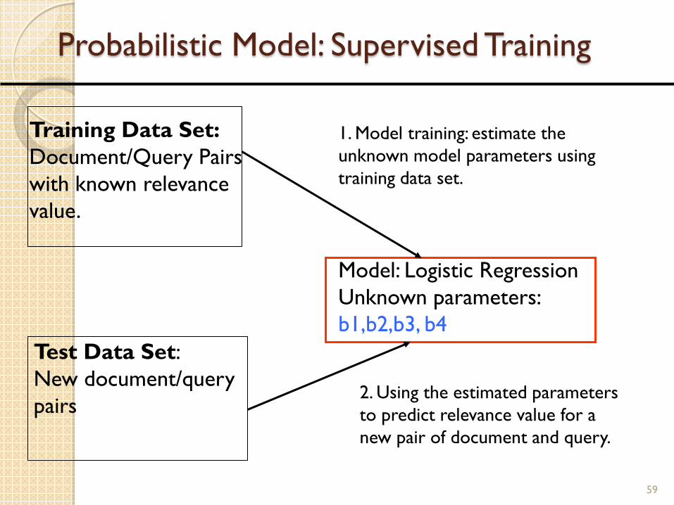
Probabilistic Model: Supervised Training

Model: Logistic Regression Unknown parameters: b1,b2,b3, b4

Training Data Set: Document/Query Pairs with known relevance value.

Test Data Set: New document/query pairs

1. Model training: estimate the unknown model parameters using training data set.

2. Using the estimated parameters to predict relevance value for a new pair of document and query.

59

Logistic Regression Method

• Model: The log odds of the relevance dependent variable is a linear combination of the independent feature variables.

• Task: Find the optimal coefficients • Method: Use statistical software package such as S-plus to

fit the model to a training data set.

relevance variable feature

variables )log()(log 1 p

ppit −=

60

Logistic regression The function to learn: f(z):

The variable z is usually defined as

◦ xi = feature variables ◦ βi=parameters/coefficients

61

Document Ranking Formula

4321 0929.01937.0330.04.3751.3),|(log XXXXQDRO ×+×−×+×+−=

N is the number of matching terms between document D and query Q.

62

Discussions Usually, terms are considered to be independent ◦ algorithm independent from computer ◦ computer architecture: 2 independent dimensions

Different theoretical foundations (assumptions) for IR ◦ Boolean model: Used in specialized area Not appropriate for general search alone – often used as a pre-filtering

◦ Vector space model: Robust Good experimental results

◦ Probabilistic models: Difficulty to estimate probabilities accurately Modified version (BM25) – excellent results Regression models:

Need training data Widely used (in a different form) in web search Learning to rank (a later lecture)

More recent model on statistical language modeling (robust model relying on a large amount of data – next lecture)

63