UNIVERSITY OF TARTU

School of Economics and Business Administration

Chair of Finance and Accounting

Martin Promen

TRADING TRENDS USING FIBONACCI CORRECTION

LEVELS AND JAPANESE CANDLESTICK PATTERNS IN

THE EXAMPLE OF STANDARD & POOR'S 500 INDEX

Bachelor Thesis

Thesis supervisor: Allan Teder, MA

Tartu 2018

Recommended for defense ......................................................................

(supervisor’s signature)

Accepted for defense “ “ ............................... 2018

Head of Chair, Chair of Finance and Accounting ............................................................

(Head of Chair’s name and signature)

I have written the Bachelor thesis independently. All works and major viewpoints of the

other authors, data from other sources of literature and elsewhere used for writing this

thesis have been referenced.

..............................................................................

(Author’s signature)

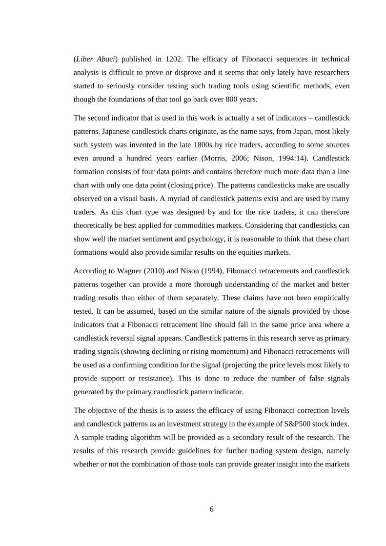
TABLE OF CONTENTS

INTRODUCTION ............................................................................................................ 5

1. CANDLESTICK PATTERNS AND FIBONACCI CORRECTION LEVELS IN

INVESTMENT STRATEGIES ........................................................................................ 8

1.1 Candlestick Pattern Formations in Technical Analysis ........................................... 8

1.2. Fibonacci Correction Levels in Technical Analysis ............................................. 16

2. EMPIRICAL TESTING OF FIBONACCI RETRACEMENTS AND CANDLESTICK

PATTERNS WITH A STRATEGY EXAMPLE ........................................................... 24

2.1. Data and Methodology ......................................................................................... 24

2.2. Testing the Candlestick Pattern Based Strategy ................................................... 28

2.3. Testing the Candlestick Pattern Strategy in Conjunction with Fibonacci Correction

Levels .......................................................................................................................... 31

CONCLUSIONS ............................................................................................................. 39

REFERENCES ................................................................................................................ 42

APPENDIXES ................................................................................................................ 45

Appendix 1. ................................................................................................................. 45

Appendix 2. ................................................................................................................. 52

Appendix 3. ................................................................................................................. 53

KOKKUVÕTE ................................................................................................................ 54

5

INTRODUCTION

In the times of computer trading and abundant information, banks and investment funds

use intricate computer algorithms to predict price movements on the markets. These

institutions are in a great need to constantly improve their trading systems and strategies

which can outperform the market not only marginally but produce a sizeable profit for

their stakeholders. At the same time, non-institutional investors (namely investors trading

self-accrued funds) who are far less researched are avid users of complex charting

analysis to either generate or confirm their trading decisions (Roscoe et al., 2009). The

testing and evaluation of such a charting strategy is the aim of this research. Such

algorithm, if proved profitable, can help traders around the world, both institutional and

private, to develop their own custom trading systems based on current market trends and

psychology.

Mayall (2006) has divided charting-based trading (sample of non-professionals) into four

rough categories which range from “scientific” system where traders try to eliminate as

much human contact with trading decisions as possible to “trading as an art” where visual

observations and trader intuition play a central role in decision making. This

nomenclature was later formalized by Roscoe and Howorth (2009) along with

conclusions that the interpretative activity by traders and investors plays an important role

in the efficacy of technical analysis (charting). They also suggested that charting has

power and importance to users as a heuristic device, regardless of its effectiveness in

generating profits.

The trading method tested in this work explores the non-interpretative charting style

(decisions based on a computer algorithm) and is based on two seemingly very different

indicators. One of these indicators is Fibonacci correction levels, which are based on the

works of Leonardo Fibonacci, namely his renowned work “The Book of Calculation”

6

(Liber Abaci) published in 1202. The efficacy of Fibonacci sequences in technical

analysis is difficult to prove or disprove and it seems that only lately have researchers

started to seriously consider testing such trading tools using scientific methods, even

though the foundations of that tool go back over 800 years.

The second indicator that is used in this work is actually a set of indicators – candlestick

patterns. Japanese candlestick charts originate, as the name says, from Japan, most likely

such system was invented in the late 1800s by rice traders, according to some sources

even around a hundred years earlier (Morris, 2006; Nison, 1994:14). Candlestick

formation consists of four data points and contains therefore much more data than a line

chart with only one data point (closing price). The patterns candlesticks make are usually

observed on a visual basis. A myriad of candlestick patterns exist and are used by many

traders. As this chart type was designed by and for the rice traders, it can therefore

theoretically be best applied for commodities markets. Considering that candlesticks can

show well the market sentiment and psychology, it is reasonable to think that these chart

formations would also provide similar results on the equities markets.

According to Wagner (2010) and Nison (1994), Fibonacci retracements and candlestick

patterns together can provide a more thorough understanding of the market and better

trading results than either of them separately. These claims have not been empirically

tested. It can be assumed, based on the similar nature of the signals provided by those

indicators that a Fibonacci retracement line should fall in the same price area where a

candlestick reversal signal appears. Candlestick patterns in this research serve as primary

trading signals (showing declining or rising momentum) and Fibonacci retracements will

be used as a confirming condition for the signal (projecting the price levels most likely to

provide support or resistance). This is done to reduce the number of false signals

generated by the primary candlestick pattern indicator.

The objective of the thesis is to assess the efficacy of using Fibonacci correction levels

and candlestick patterns as an investment strategy in the example of S&P500 stock index.

A sample trading algorithm will be provided as a secondary result of the research. The

results of this research provide guidelines for further trading system design, namely

whether or not the combination of those tools can provide greater insight into the markets

7

and be applicable as a profitable strategy. In order to reach that objective, it is necessary

to fulfill the following tasks:

Analyze the nature and underlying principles of candlestick patterns for

understanding their ways of describing and interpreting data from the markets;

Analyze and describe Fibonacci correction levels, the different theories of

applying them in technical analysis;

Review other works and scientific papers published on the topics;

Test the predictive power of candlestick patterns without other technical

indicators;

Test whether applying Fibonacci retracement levels to candlestick analysis

provides greater predictive value and creating a sample portfolio.

This work is divided into two main chapters: the first chapter describes the theoretical

background and previous research on the topic, the second chapter contains empirical

research conducted on the historical price data of the S&P500 index.

Keywords: Fibonacci retracements, candlestick patterns, investment strategy, Elliott

waves, technical analysis, charting.

8

1. CANDLESTICK PATTERNS AND FIBONACCI

CORRECTION LEVELS IN INVESTMENT STRATEGIES

1.1 Candlestick Pattern Formations in Technical Analysis

To understand why candlestick patterns provide important predictive information it is

first necessary to understand how they are formed in the first place. They are very similar

to bar charts, a chart type used long before candlestick charts were introduced to the

western world (Nison, 1994)1. A candle consists of four data points: open, high, low,

close. Open and close determine the color of the candle and form also the “body” of the

candle. If the candle closes below the opening price then it has a red body and if the

closing price is above open then the candle is red2. This makes reading candlestick charts

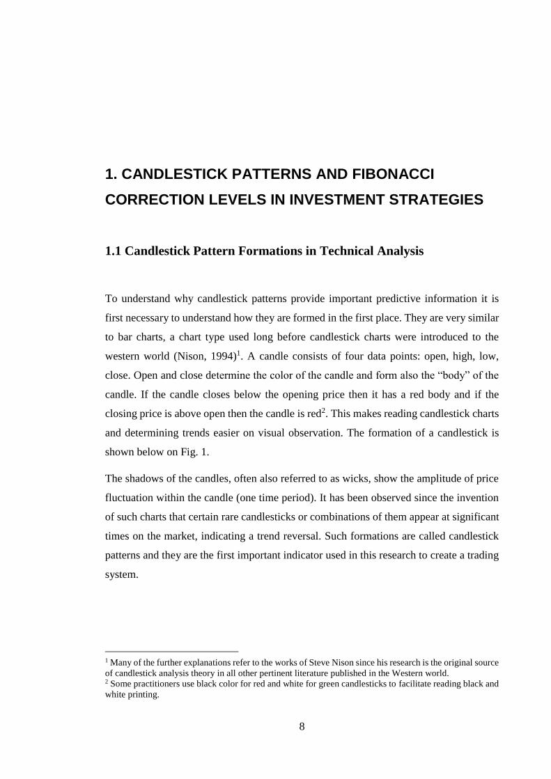
and determining trends easier on visual observation. The formation of a candlestick is

shown below on Fig. 1.

The shadows of the candles, often also referred to as wicks, show the amplitude of price

fluctuation within the candle (one time period). It has been observed since the invention

of such charts that certain rare candlesticks or combinations of them appear at significant

times on the market, indicating a trend reversal. Such formations are called candlestick

patterns and they are the first important indicator used in this research to create a trading

system.

1 Many of the further explanations refer to the works of Steve Nison since his research is the original source

of candlestick analysis theory in all other pertinent literature published in the Western world. 2 Some practitioners use black color for red and white for green candlesticks to facilitate reading black and

white printing.

9

Figure 1. Anatomy of candlesticks. Made by the author

The major advantage of candlestick charts is that they show the momentum of price

moves and are visually easier to understand than bar charts or line charts (Fischer and

Fischer, 2003:83; Schlossberg, 2006). For the purposes of an automated trading program

it is only necessary to have the four data points (open, high, low, and close) but since the

pattern theory was developed in Japan using candlestick charts then for the purposes of

all related research and visualizations, candlestick charts should be used.

Data on the efficacy of candlestick pattern formations varies greatly and should be taken

with a grain of salt. As candlesticks are seldom used alone in making trade decisions then

all findings regarding the efficacy of those patterns are inconclusive for trading purposes

but are indicative for the selection of patterns which are theoretically more likely to yield

profitable results when used in conjunction with other indicators. Although Robert and

Jens Fischer (2003:84-88) found in their work that candlesticks can be profitable on their

own, they also pointed out a research by Andre Rogalski who researched Dax 30 Futures

Index and Euro-Bund Futures and found profit potential only in bullish engulfing pattern,

hammer and hanging man (Rogalski 2001, referenced through Fischer and Fischer,

2003:85).

Maiani (2002) who researched US stocks and bonds over a period of 15 to 20 years found

that the more rarely a candlestick formation appears the more likely it is to be accurate.

For example a formation known as “Three Black Crows” resulted in the market rising the

following day in 67.65% of the cases but such a formation was only found on 102

Upper wick

Close

Close

Low Low

Open

Open

High

Open

Open

Real Body

Lower wick

High

10

occasions out of the total of over 6 million candlestick patterns observed. The limitation

of Maiani’s work is that he evaluated the profitability of candlesticks based on the day

immediately following the formation. This produces some misleading results, such as the

case of the Three Black Crows which is a bearish signal (Nison, 2003:94) but according

to Maiani it resulted in a bullish move in the market the following day. Considering that

the patterns consist of three long bearish candlesticks (each candle closing at or near the

session lows) then it is perfectly natural that the price will find support and bounce back

after such an intensive period of sellers dominating the market.

Examples of different research methods include Marshall et al (2006) who used the

bootstrapping methodology to simulate market data and research ten years of Dow Jones

Industrial Average price data. He concluded that candlestick patterns produce no value

(even before including transaction costs) for the investor. A year later he conducted a

similar research on Japanese stock market data and arrived at the same conclusions

(Marshall et al, 2007). In both studies, a ten-day moving average was used to determine

trends and all positions opened based on those signals were closed ten days after opening.

The way of determining profitable trades in those studies leaves one to wonder how close

to the real world are these models. It is probably safe to assume that traders would take

profits or cut losses depending on the price scale, not time.

However, the use of ten days in candlestick analysis is justified. The signals given by

candlestick formations are effective in the short term, on average indeed about ten days

(Nison, 1991:236-238). These results were also supported by an empirical study by Chen,

et al. (2016). Reality is however more complex and the time period while positions are

kept open depend from various biased factors, such as investor’s mood, volatility of the

markets, momentum (or duration of the trend for trend traders), position size and of course

price movements. The “ten-day rule” is taken into consideration in this paper to assess

the potential profitability of candlestick analysis. The average closing price for the ten-

day period following a signal is calculated and stop-loss rules set. If that average is then

higher (or lower, depending on the direction of the trade) than the opening price of the

day following a candlestick signal then a trade is considered potentially profitable.

It should also be taken into consideration that algorithms used to identify chart patterns

according to chosen rules are rigid which eliminates any bias a trader might have when

11

observing chart patterns visually. It means that a case of an otherwise valid and equally

reliable pattern when it is even slightly off the input parameters will be overlooked by the

search program but not by traders searching for these patterns manually. In case of

trading, a certain degree of trader bias can be beneficial for the result and may be the

reason why we often see practitioners achieving better results than academics.

Practitioners like Boris Schlossberg (2006:43) point out that candlestick analysis

proponents often attribute almost “mystical powers” to candlestick analysis when

describing their predictive power but in reality, they only have value when used together

with other indicators. This may well hold true considering empirical evidence that renders

candlestick analysis as stand-alone indicator unprofitable. The reason why it is considered

profitable by its proponents can be thanks to tacit knowledge a trader possesses, some

intuition developed over years of experience and practice. This opinion is further

supported by Roscoe et al. (2009) who speculated it could be the reason why technical

analysis has considerable effectiveness among practitioners in the first place.

The following paragraphs describe the visual properties of various candlesticks that were

chosen to be tested with and without the addition of Fibonacci lines. The choice of

candlesticks for this particular work is largely subjective by the author but does try to

give a representative sample of single- and multiple line formations that have in previous

works been deemed potentially profitable (see Maiani, 2002; Chen et al, 2016; Fischer

2003). The choice is also based on the rarity of the patterns and very rare patterns have

been mostly excluded (based on the number of occurrences determined by Maiani, 2002).

The majority of the patterns is formed by no more than two candlesticks.

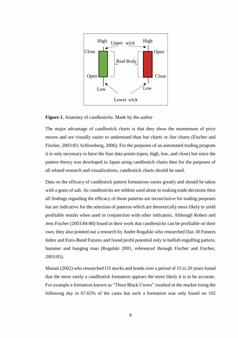
Doji is a candle formation where the period opening price and closing price are the same

or very close whereas the wicks of the Doji candle can vary in length. A typical Doji

candle (where open and close prices do not exactly match) is shown on Figure 2.

Figure 2. Bullish (green) and bearish (red) Doji candlesticks. Perfect Doji on the right.

Made by the author.

12

Instead of classic “ideal” Doji candles where open and close match perfectly, a more

liberal version of the Doji is used in this research. It means that the required distance

between open and close price does not have to be zero but the Doji body to length ratio

has to be less or equal to 0.1. Such concession can be made since the predictive power of

Doji candles is derived from the underlying market psychology. Extreme proximity of

open- and close prices indicates indecisiveness in the markets, it shows that the traders

and market makers have not yet “decided” which way the market will go or should be

going. As any simple observation can show, all financial markets will sooner or later

experience significant fluctuations in prices.

According to Maiani (2002) who researched over 20 years of US stock and bond data,

Doji candle formations did not have any predictive power in terms of market direction.

He concluded that 42.28% of the times the market was up the following day and in

42.48% of the cases down. This information has no value in terms of price prediction

since Doji in itself is not a trend predictive pattern. It is simply an indicator that both

forces are present and equally strong in the market since the open and close prices are

extremely close to each other. However, Doji can be a useful tool in determining when a

trend or correction is exhausted. According to Nison (2003:52), Doji in a downtrend has

less value than Doji in an uptrend. This theory is further examined in Chapter 2.

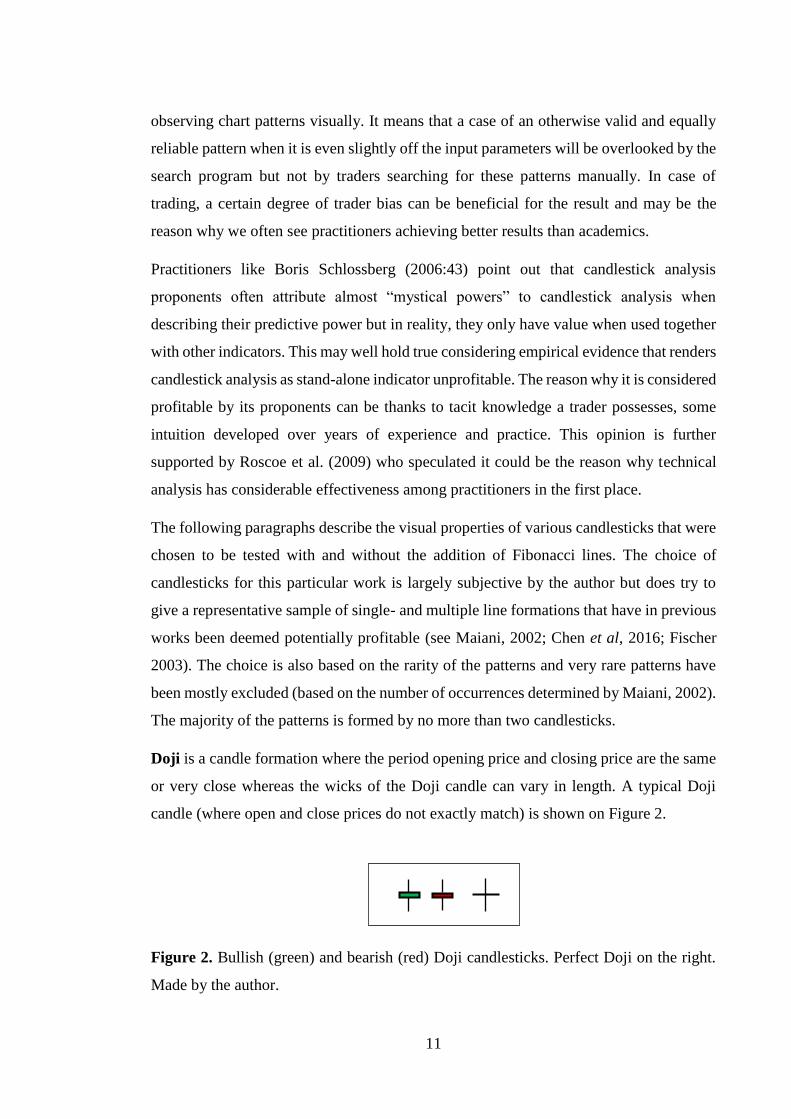
There are two special cases of Doji patterns which are trend predictive. They occur when

one wick of the candle is significantly long while the other is very tiny or nonexistent (see

Fig. 3). When the long wick is located on top it is called Gravestone Doji, when on the

bottom then Dragonfly Doji.

Figure 3. Dragonfly Doji candle (left) and Gravestone Doji (right). Made by the author.

The predictive power of these special Doji candles stems from their appearance in a trend.

Dragonfly Doji at the end of a downtrend is extremely bullish and Gravestone Doji at the

end of an uptrend is bearish (Nison, 1991:159). The length of the longer wick can be

13

however long (the longer the better) but shorter wick has to be nonexistent (maximum

allowed wick length used here is again 1/10 of the candle length).

Hammer and Hanging Man are both candlesticks with small real bodies but long lower

wick (see Fig. 4). As described by Nison (1994) the term “Hammer” comes from the

market seemingly “hammering out a base” and “Hanging Man” from its resemblance to

a man hanging down from a top. These names make it easy to remember: Hammer is a

bullish signal, Hanging Man bearish. The color of the real body has no importance for the

validity of the pattern. The restrictions used in the identification of Hammer and Hanging

man are identical: the minimum lower wick length has to be 2/3 of the whole candle

length (high – low), maximum allowed upper wick length is 10% of the candle length and

minimum candle body length 10% of the total as well.

Figure 4. Hammer (left) and Hanging Man (right). Made by the author.

These patterns both need a trend to be valid indicators. It is also noted by Nison (1994:54)

that the first price bounce from the Hammer may fail due to selling pressure still present

in the market but the price usually comes back down to test the Hammer’s support.

Inverted Hammer and Shooting Star are once again the same formation differentiated

only by the trend in which they occur. They are like mirrored images of Hammer and

Hanging Man (Fig. 4). Inverted Hammer in a downtrend predicts a soon-starting uptrend,

just like Hammer itself. Shooting Star appearing in an uptrend shows exhaustion of the

trend and imminent reversal. The parameters for identifying those patterns are the same

as for Hammer and Hanging Man.

Marubozu, sometimes referred to as belt hold line, is a candlestick with a full candle

body and either no wicks at all or they are minuscule compared to the full length of the

candle. Since the more liberal interpretation of these formations by Nison would identify

14

an excess of signals in the daily time frame then a stricter version is used here. Period

high must equal to its close in case of a white Marubozu (bullish) and low must be equal

to close in case of a black Marubozu (bearish). In other cases, maximum allowed wick

length is 1/10 of total length.

Harami (see Fig. 5) forms when a large candlestick totally engulfs a small following

candle. Bearish and bullish versions of this formations exist and they are both relevant

only when found in a trend.

Figure 5. Bullish Harami in a downtrend (S&P500, D). Made by the author.

In 48.43% of the cases, a Bullish Harami predicts a positive trading day and Bearish

Harami predicts a negative trading day with 50.8% accuracy (Maiani, 2006).

Harami’s “cousin” is the Engulfing Pattern which is composed of the same elements as

Harami but in a different order. In the Engulfing Pattern, the long candle appears after the

short candle, making it a mirror image of the Harami. The Bullish Engulfing pattern was

one of the few profitable patterns in a research concerning European and German bonds

(Rogalski 2001, referenced via Fischer and Fischer, 2003:85).

Piercing Pattern and Dark Cloud Cover form when the second of the two candles

penetrates more than half of the preceding candle’s real body while opening at or

above(below) the previous candle’s closing price. The candles are of altering color – in

Piercing Pattern a green candle follows previous red candle and in Dark Cloud formation

a red candle “covers” most of the previous green candle. For both versions, a preceding

trend is necessary for the validity of the pattern.

15

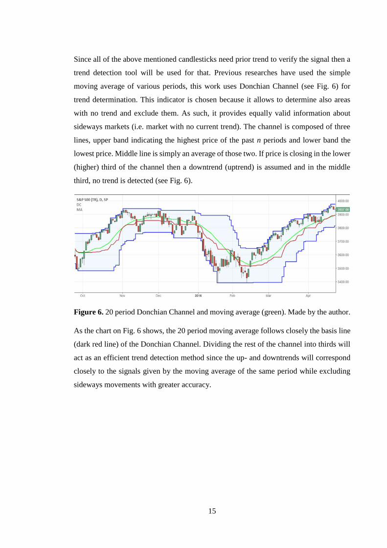
Since all of the above mentioned candlesticks need prior trend to verify the signal then a

trend detection tool will be used for that. Previous researches have used the simple

moving average of various periods, this work uses Donchian Channel (see Fig. 6) for

trend determination. This indicator is chosen because it allows to determine also areas

with no trend and exclude them. As such, it provides equally valid information about

sideways markets (i.e. market with no current trend). The channel is composed of three

lines, upper band indicating the highest price of the past n periods and lower band the

lowest price. Middle line is simply an average of those two. If price is closing in the lower

(higher) third of the channel then a downtrend (uptrend) is assumed and in the middle

third, no trend is detected (see Fig. 6).

Figure 6. 20 period Donchian Channel and moving average (green). Made by the author.

As the chart on Fig. 6 shows, the 20 period moving average follows closely the basis line

(dark red line) of the Donchian Channel. Dividing the rest of the channel into thirds will

act as an efficient trend detection method since the up- and downtrends will correspond

closely to the signals given by the moving average of the same period while excluding

sideways movements with greater accuracy.

16

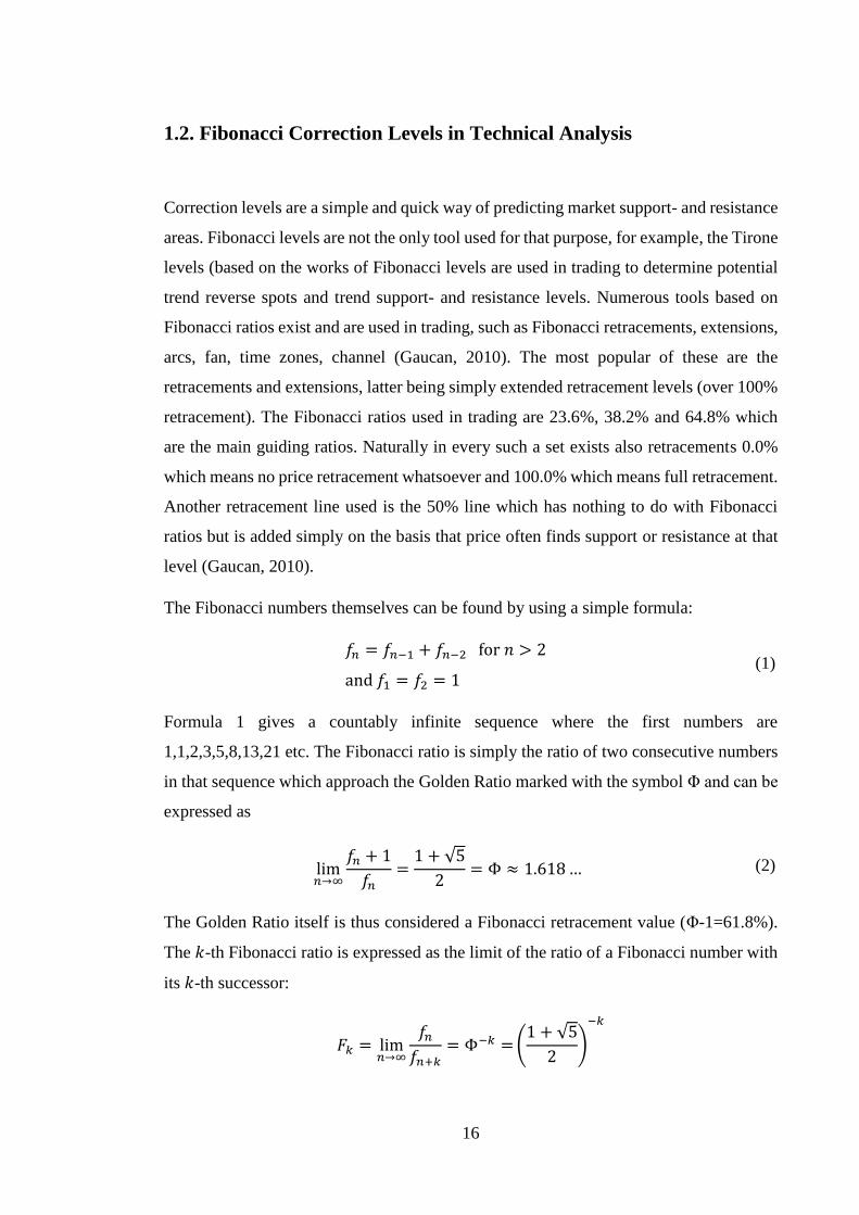
1.2. Fibonacci Correction Levels in Technical Analysis

Correction levels are a simple and quick way of predicting market support- and resistance

areas. Fibonacci levels are not the only tool used for that purpose, for example, the Tirone

levels (based on the works of Fibonacci levels are used in trading to determine potential

trend reverse spots and trend support- and resistance levels. Numerous tools based on

Fibonacci ratios exist and are used in trading, such as Fibonacci retracements, extensions,

arcs, fan, time zones, channel (Gaucan, 2010). The most popular of these are the

retracements and extensions, latter being simply extended retracement levels (over 100%

retracement). The Fibonacci ratios used in trading are 23.6%, 38.2% and 64.8% which

are the main guiding ratios. Naturally in every such a set exists also retracements 0.0%

which means no price retracement whatsoever and 100.0% which means full retracement.

Another retracement line used is the 50% line which has nothing to do with Fibonacci

ratios but is added simply on the basis that price often finds support or resistance at that

level (Gaucan, 2010).

The Fibonacci numbers themselves can be found by using a simple formula:

𝑓𝑛 = 𝑓𝑛−1 + 𝑓𝑛−2 for 𝑛 > 2

and 𝑓1 = 𝑓2 = 1

Formula 1 gives a countably infinite sequence where the first numbers are

1,1,2,3,5,8,13,21 etc. The Fibonacci ratio is simply the ratio of two consecutive numbers

in that sequence which approach the Golden Ratio marked with the symbol Φ and can be

expressed as

lim𝑛→∞

𝑓𝑛 + 1

𝑓𝑛=

1 + √5

2= Φ ≈ 1.618 …

The Golden Ratio itself is thus considered a Fibonacci retracement value (Φ-1=61.8%).

The 𝑘-th Fibonacci ratio is expressed as the limit of the ratio of a Fibonacci number with

its 𝑘-th successor:

𝐹𝑘 = lim𝑛→∞

𝑓𝑛

𝑓𝑛+𝑘= Φ−𝑘 = (

1 + √5

2)

−𝑘

(1)

(2)

17

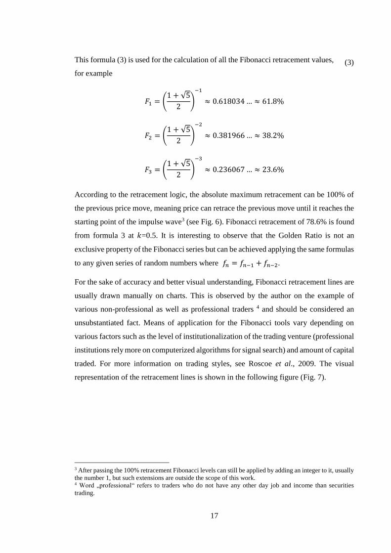
This formula (3) is used for the calculation of all the Fibonacci retracement values,

for example

𝐹1 = (1 + √5

2)

−1

≈ 0.618034 … ≈ 61.8%

𝐹2 = (1 + √5

2)

−2

≈ 0.381966 … ≈ 38.2%

𝐹3 = (1 + √5

2)

−3

≈ 0.236067 … ≈ 23.6%

According to the retracement logic, the absolute maximum retracement can be 100% of

the previous price move, meaning price can retrace the previous move until it reaches the

starting point of the impulse wave3 (see Fig. 6). Fibonacci retracement of 78.6% is found

from formula 3 at 𝑘=0.5. It is interesting to observe that the Golden Ratio is not an

exclusive property of the Fibonacci series but can be achieved applying the same formulas

to any given series of random numbers where 𝑓𝑛 = 𝑓𝑛−1 + 𝑓𝑛−2.

For the sake of accuracy and better visual understanding, Fibonacci retracement lines are

usually drawn manually on charts. This is observed by the author on the example of

various non-professional as well as professional traders 4 and should be considered an

unsubstantiated fact. Means of application for the Fibonacci tools vary depending on

various factors such as the level of institutionalization of the trading venture (professional

institutions rely more on computerized algorithms for signal search) and amount of capital

traded. For more information on trading styles, see Roscoe et al., 2009. The visual

representation of the retracement lines is shown in the following figure (Fig. 7).

3 After passing the 100% retracement Fibonacci levels can still be applied by adding an integer to it, usually

the number 1, but such extensions are outside the scope of this work. 4 Word „professional“ refers to traders who do not have any other day job and income than securities

trading.

(3)

18

Figure 7. Fibonacci retracement lines on the weekly chart of Halliburton (HAL). Made

by the author.

After a clear uptrend that lasted for about two years, HAL peaked at $74 and started a

downward trend in July 2014. The retracement lines on the graph are applied from the

highest high of July 2014 at $74 to the lowest low in January 2016 when Halliburton’s

stock was worth less than $28. Following price action shows some price consolidation

around the 38.2% retracement line and a continuation of the downtrend near 61.8%

retracement level while not fully respecting it and closing above the line. However, in

mid-August 2017 the long price drop found some support at the 23.6% retracement

without closing below the line.

Although the example above uses a weekly chart, Fibonacci retracement tool can be used

successfully on any time frame and asset (Boroden, 2008:6; Greenblatt, 2007; Kempen,

2016). The key to successful trade setups is in identifying the right swing highs and lows

for drawing the retracement lines. There is no consensus on what constitutes as the

“correct” wave. Practitioners apply different methods and timeframes and recommend

applying the correction levels “differently than the majority” without specifications

(Williams, 2012:28). Hartle (1993) and Krausz (1998) concluded that although Fibonacci

indicators (including retracements) are widely used in practice, they are still almost

always used together with other technical analysis tools and indicators as a component of

some multi-indicator algorithm.

These time frames pose some difficulties for accurate computer algorithms since multiple

time frames should be used at once – for example weekly to determine the general trend

19

the market follows at any moment, daily charts to determine short-term trends and

significant price moves and also intraday charts (for example hourly chart) to find the

best entry point for the trade. Time frames should be chosen based on the desired duration

of holding a position open. To simplify that process of identifying highs and lows for the

purposes of this research, the stock index will be simplified to straight lines based on

high-low price data. In this paper, only daily data is used for trend determination since it

was recently brought out by Kempen (2016) that Fibonacci retracements are scale-

invariant.

It is important to bear in mind that trades should follow the current price trend of an asset.

It is, of course, possible to execute successful trades countering the trend since the prices

always go through a certain number of corrections before continuing in the general

direction but such trades are riskier (Michalowski, 2012:36). The general principles of

how any market behaves in terms of price and time come from Ralph Nelson Elliott who

published his theory in the book “The Wave Principle” (1938). Elliott claimed that price

movements on the stock market follow a certain wave pattern which is repetitive in form

but not always in time and amplitude (Frost and Prechter, 2005:19). These patterns are

now commonly referred to as Elliott waves. The idealistic form of the wave patterns is

shown in Figure 8.

A market cycle consists of numerous waves of various degree which contain similar

waves of lower degrees. This models the seemingly complex stock market into a self-

repeating fractal which can be used to make predictions about future movements. Fig. 8

shows four types of Elliott waves where wave I is the motive or impulse wave and II the

following corrective wave. Following subdivision consists of five motive waves marked

[1] through [5] followed by same degree corrective waves marked [A] through [C].

Analysts like Frost and Prechter (“Elliott Wave Principle”) who are sometimes referred

to as “Elliott wave purists” do not discuss the Fibonacci connection to Elliott waves at all

and consider only the wave count and counting rules as their primary indicator. Others

such as Bulkowski (2005) and Fischer (2003) have added Fibonacci indicators to the mix

based on observations that the Elliott correction waves tend to retrace the length of the

previous impulse wave that is close to retracement values calculated from Fibonacci

numbers.

20

Figure 8. Complete market cycle in Elliott waves. Source: Frost and Prechter, 2005:25

Inside the 8 largest subdivision waves are 34 even smaller motive and corrective waves

that are combined of 144 even smaller subdivisions which all follow the same 5+3 pattern.

Frost and Prechter (2005) speculate that such combination of five waves to progress

together with three waves to regress exist in that ratio because it is the minimum

requirement to achieve both fluctuation and progress, making it the most efficient form

of punctuated progress.

There are three main principles of such movement, described by R. N. Elliott as follows:

Wave 2 never moves beyond the starting point of wave 1;

Wave 3 is never the shortest wave;

Wave 4 does not enter (close) in the price range of wave 1.

It has been highlighted by Robert R. Prechter, Jr. in his article “Elliott Waves, Fibonacci

and Statistics” (2005) that R. N. Elliott himself never used the Fibonacci ratios for

forecasting and never made generalizations about retracements. Nevertheless,

practitioners and theorists like Tom Joseph (1999), Robert and Jens Fischer (2003), Kathy

Lien (2004) and many others have recommended using Fibonacci retracement values in

one way or another to predict the wave pattern formations. The most common way of

integrating Fibonacci retracements into Elliott wave theory seems to be using certain

21

retracement values to determine a resistance area where the trend is expected to either

break or continue after a pullback (i.e. correction wave). Bulkowski (2005) went a step

further with Fibonacci Elliott wave connection and discussed Fibonacci price targets

which he calculates based on Fibonacci multiples (extensions as well as retracements).

This gives reason to assume that Fibonacci retracements can help other technical analysis

tools (such as candlestick patterns) to be more efficient since for every significant price

move it gives a finite number of potentially significant support- or resistance levels.

Based on a recent research (Kempen, 2016), active trends will continue with almost 59%

probability (retracement ends before retracing 100% of the previous move). The concept

of trend continuation being more likely than trend break is also the basic tenet of all trend

following strategies in general. It makes sense looking at the basic Elliott 5-wave motive

pattern – there are more and stronger moves that go with the trend (3 waves) than there

are movements against it (2 correction waves). If Elliott wave theory holds true and we

assume equal length for all the 5 waves then it is clear that 60% of all the movement is in

the direction of the underlying trend, a result which interestingly is very similar to the

trend continuation probability determined by Kempen.

Combining the knowledge that trends are more likely to continue than break and that

every market impulse is followed by a correction gives a rather good idea where to enter

the market for a trend following trade. To make a profitable trade, one should open a

position at or near the end of a correction wave and hold it until trend continues its

movement in the original direction. This holds true for both uptrends and downtrends. In

such way investor or trader can put his or her faith in the greater probability that trend

continues. If a trader is good at determining which moves are correctional then such

approach is poised to generate profits over time.

Unfortunately, predicting the points where market finds support or resistance as well as

determining the current Elliott wave in which the market moves can prove to be a very

difficult challenge. This is where many traders seek help from technical analysis. Wagner

(2010) combined Elliott wave theory with Fibonacci retracement lines and candlestick

patterns to predict gold prices. His way of analysis did not include any computerized

algorithms, he counted the waves and patterns visually from the chart (a method known

as “chart-seeing” (Roscoe et al., 2009)). Other researchers (e.g. Kempen, 2016;

22

Bhattacharya et al., 2006) have used purely statistical methods without visual

observations of the price charts to analyze the efficacy of Fibonacci lines. Not

surprisingly, practitioners who use visual observations for short-term analysis of a price

chart always present positive examples while statistical analysis is rarely yielding any

evidence that Fibonacci retracements have value for price predictions. Their success can

be attributed to two factors – careful selection of sample data with selective presentation

of results and possession of tacit knowledge gained from years of experience in securities

trading (Roscoe et al., 2009). However, it is possible (and nothing in science rules it out)

that the success of practitioners is achieved purely on technical analysis.

Michalowski (2012:37) reported that in trending markets, 38.2% and 50% retracements

are the most relevant Fibonacci retracement levels and called the area between those

levels “Correction Zone”. He explained that if that zone holds the price then the trend is

very likely to continue since trend makers are committed. For trend determination,

Michalowski used the simple moving average (100 period). Williams (2012) on the other

hand deemed the 38.2% and 61.8% retracements most useful and profitable. He provided

the following guidelines for both values:

For 38.2% retracement:

If price holds at the retracement, then the prior move is strong and the counter

move will be also strong;

Retracement after a strong move is usually followed by a move to a new high;

After a strong decline, if retracement holds, a new low is typically created.

For 61.8% retracement:

If price reaches this retracement, prior move has been weak and as a result, counter

move will be weak;

The chance of exceeding the prior high when price hits the retracement after a

strong move is 1/3;

The first retracement after a strong move is considered a trade signal in the main

trend direction but exiting the position should be considered when price nears its

previous high or low.

23

The frequent change of direction (i.e. continuation of the previous trend) on the 61.8%

retracement line was also noted on the US and Lithuanian stock markets (Baranauskas,

2011). From those observations the following conclusion can be made about the

retracement lines: signals forming at lower value retracements (such as 23.6% and 38.2%)

have greater potential for successful trend trades than higher value retracements. It seems

that when it comes to deciding which retracements perform best, no consensus has yet

been reached by practitioners.

Kempen (2016) who tested Fibonacci retracement levels on different scale trends did not

find any evidence that some retracement levels performed better than others, but noted

that price reversal is more likely around the 50% retracement. His analysis was strictly

statistical and did not involve the tacit knowledge a lifelong trader might have, meaning

the degree of bias has been kept to minimum. He further concluded that Fibonacci

retracements are scale-invariant, meaning that their predictive power does not change

when switching from major trends to short-term trends. This discovery is taken into

consideration for the empirical analysis conducted in this research. Author proposes that

Fibonacci retracement lines are used by traders in similar way as technical analysis in

general (according to Roscoe and Howorth (2009)) – as a heuristic device to facilitate

decision making and provide support to previous analysis. This does not imply that they

would not have any objective value, but it appears that the subjective value is greater.

That deduction is based on the lack of uniformity in applying the tool and interpreting it.

Fibonacci retracement lines are calculated in the empirical part of this researcg by using

significant highs and lows in the S&P 500 price series which are obtained by applying

the ZigZag tool. The tool smoothes out price movements to straight lines with specified

sensitivity resulting in a series of angled lines. The sensitivity used is 2.5% of the previous

price move. This means that every price movement smaller than 2.5% will be eliminated

from the series and the lines between remaining extreme points are interpolated. The

result is a series that contains only straight lines which are located between local maxima

and minima points. Those points are then located in the series and they equal to the

S&P500 High-Low prices.

24

2. EMPIRICAL TESTING OF FIBONACCI

RETRACEMENTS AND CANDLESTICK PATTERNS

WITH A STRATEGY EXAMPLE

2.1. Data and Methodology

The most important part of creating an efficient trading system is the process of back-

testing which means running a retrospective simulation with historical market data to

ascertain whether a combination of indicators and their settings would have generated a

sufficient amount of profitable trades. The results of that simulation are what determines

the efficacy of a technical analysis indicator. The data used for the analysis is obtained

from Yahoo databases (www.finance.yahoo.com) by importing the dataset directly into

RStudio5 using the analysis package “quantmod”. The data matrix contains six columns

of information: open price, daily high, daily low and close price, trading volume and

adjusted price which in the sample is equal to the daily closing price. The index is

composed of the 500 largest U.S. companies and is regarded by Investopedia as one of

the best representations of the U.S. stock market and economy.

The data spans from January 3rd 2007 to November 17th 2017 containing 10 years and 10

months of historic price data on the index. Weekends and US national holidays (such as

Independence Day, Labor Day and Christmas) are excluded since the stock markets were

closed and no trading took place. Since candlestick patterns were introduced to the

western world in the early 1990s and OHLC stock data also made available around that

time then traders have had the chance to implement candlestick trading patterns only from

5 R is an open source software and programming language for statistical computing, RStudio is a software

application for R.

25

the start of 1992 (Marshall, 2006). Therefore it can be assumed that data prior to that

decade would perform worse in back testing since it is missing the “self-fulfilling

prophecy” 6 factor since candlestick patterns were largely unknown to traders in the US.

Daily index data is used in this particular research since an investment strategy is tested

and not day trading strategy then such a time frame contains less random noise and

whiplash which is widely present in smaller time frames. For day traders, intraday charts

should be used to test the efficacy of Fibonacci and candlestick pattern strategy.

Both short and long positions will be considered to analyze the efficacy of the investment

strategy in up- and downtrends. Long position means buying the security, anticipating

further price increase so the assets can be sold at a later time for higher price than at the

time of the purchase. Short position (selling short) involves borrowing, selling and buying

back shares in the hope that price will decrease and the assets sold could be bought back

cheaper at a later date.

Using the two chosen indicators it is necessary to have three conditions fulfilled in order

for a buy or sell signal to be generated. These are:

1. Market must be in either a down- or an uptrend defined by the section of the

Donchian Channel. Location determined by the closing price of the last candle in

the formation ;

2. Candlestick pattern formation is required (see Chapter 1.1), either bullish (in a

downtrend) or bearish (in an uptrend);

3. Candlestick formation (body of the last candle in the formation) must exist on any

of the five Fibonacci correction line described in Chapter 1.2.

It is important to bear in mind that candlestick patterns are highly visual tools and even

though it is perfectly possible to create a computerized algorithm for finding formations

similar to these patterns, the final decision for entering a position should be assessed

individually by the investor based on his risk tolerance, trading style and of course by

other external factors the investor deems relevant in a particular asset at a given moment.

Since the profit-taking from trades would vary from person to person then no strict targets

or rules have been used at first. This is to add objectivity to this research and not tie it to

6 Idea that the predictive power of an indicator is derived from traders acting upon signals of that indiator.

26

strict trading rules which are very different among investors and traders. Only potential

profitability is assessed based on the short-term nature of candlestick patterns. It means

that a signal is considered profitable if and when the average closing price of a ten-day

period following the signal is higher or lower (depending on the direction of the trade)

than the opening price of the day immediately following the signal. Opening prices are

used since it is assumed that the position would be opened as soon as possible following

a relevant signal. Closing prices are used for the calculation of the price average since it

is assumed (based on Marshall et al, 2007 and Chen et al, 2016) that ten days would be

the optimal period when to close the trade.

For the second part of the assessment, trades are executed based on simple trading rules

at the liberty of the author. This exercise serves as one example of how profitable this

strategy can be under only one set of conditions. It will be demonstrated only with the

combination strategy on the following conditions:

1. Positions are entered when the market opens for trading the day following a signal;

2. A stop-loss order is triggered when the market makes a move against the trade by

at least 3% counting from the highest/lowest price of the signal candle formation

Long side stop-loss 𝑆𝐿 = 𝐿𝑚𝑖𝑛 − (𝐿𝑚𝑖𝑛 ∙ 0.03)

Short side stop-loss 𝑆𝐿 = 𝐻𝑚𝑎𝑥 − (𝐻𝑚𝑎𝑥 ∙ 0.03);

3. Position is closed when price has reached a price target of 10% increase counting

from the closing price of the signal candle formation;

4. Multiple positions can be open at the same time, including simultaneous holdings

of short- and long positions;

5. Absent to signal, no funds on the dummy account will be held invested in

securities nor will they earn interests outside the S&P500 index futures.

This method is simple yet powerful – by setting the stop-loss and profit targets the same

time as position is opened the trade can only have two outcomes: either a small loss is

suffered or a sizeable profit generated. This analysis does not go into detail about where

the stop-loss and profit-taking orders should be placed since this is highly dependent on

the risk tolerance of the investor as well as the volatility of the asset (Teweles et al.,

1987:275). A stop-loss rule of 7 or 8% loss of invested capital was proposed by O’Neil

(1988:87) for equities markets but since S&P 500 is considerably less volatile than any

27

single stock then this rule would likely be inefficient. If we operate under the assumption

that a fraction of the starting capital is traded then the cumulative losses can be as

exponentially growing as potential cumulative gains. It means that according to simple

math, it takes more than a +10% gain to make up for a -10% loss since after said loss, the

account traded is smaller, hence the future gains on that +10% would be smaller. Because

of that, any outcome of any portfolio depends heavily on whether or not the first trade

was a successful one. Since it is virtually impossible to foresee this (especially when

testing an algorithm) then risk must be managed in such a way that potential gains more

than cover potential losses. On the example of O’Neil’s 7-8% stop-loss the profit target

should be significantly larger.

A “rule of thumb” was described by Linton (2010) claiming that the ideal trade is where

profit outweighs loss by a ratio of 3 to 1. This ratio is known as risk-reward ratio and

expresses how many units of money a trader is willing to risk to achieve the desired gain.

On the example of 3:1 ratio, trader risks one dollar to gain 3 (assuming operations in

dollars). Applying this math to O’Neil’s stop-loss of maximum 8% capital loss we get

that in this case, price target should be at slightly above 19% move in the predicted

direction. Considering numerous experts who have, either empirically or through

experience, claimed that candlestick signals are short-term then expecting such a

substantial move in short-term is not justified.

The knowledge that major indexes do not move as rapidly as equity shares is well known

to everyone and deductible from logic, therefore using this knowledge for setting targets

and stop-losses in back-testing is allowed. Any further calculations however (based on

the sample data) would distort the results and credibility of research since it would have

been impossible to access such data before entering the market. Considering all that, the

stop-loss rule for the purposes of the back-testing algorithm will be 3% movement against

the trade (less than half of that proposed by O’Neil) and profit target at 10%, giving a

risk-reward ratio of 3.29, slightly more favorable than Linton’s 3. This means that even

if only one trade out of three is profitable then investor will at least break even (neither

lose nor gain significant money).

In chapter 2.2 a strategy based solely on candlestick patterns is tested for potential

profitability. In chapter 2.3 candlestick patterns are used in conjunction with Fibonacci

28

correction levels and tested for potential profitability as well as real profitability on the

example of simple position entry- and exit rules. A comprehensive list of risk-adjusted

ratios (such as Sharpe ratio, Sortino ratio) and other portfolio evaluation metrics such as

standard deviation, portfolio alpha and beta will be provided in the end. All of the

calculations and analysis was conducted in R language

2.2. Testing the Candlestick Pattern Based Strategy

Researches that concentrate solely on the efficacy of candlestick patterns often return

lackluster results as observed earlier. This work will not aim to test the whole pantheon

of patterns (which there are over 40) but rather takes example from earlier works where

better performing and often occurring candlestick patterns were recognized. Patterns are

divided into two categories: single candle lines and patterns composed of two or more

candlesticks.

Single lines are patterns composed of only one candlestick. They are the most common

patterns due to their simplicity, confirmed by Maiani (2002). Such patterns always have

either abnormally long wicks on top or bottom or no wicks at all. An exception here is a

simple Doji candle where the key distinction is open and close price being extremely

close. Doji candles are also tested here using preceding trend to differentiate bullish and

bearish formations. If a Doji appears in an uptrend then it generates a sell signal and when

in downtrend then buy signal.

To assess whether or not a pattern is profitable, an average of the following 10 days is

calculated. If that average is higher (lower) than price at the time when buy (sell) signal

was generated then trade is considered potentially profitable. Closing prices were used to

calculate that average. This method is similar to the one used by Marshall (2006 and 2007)

but instead of closing the trade on the 10th day, only the possible profitability of the trade

is observed.

29

Table 1 illustrates the frequency (number of occurrences) and percentage of profitable

signals for single line candlestick formations tested.

Table 1. Single line candlestick formation profitability results. Made by the author.

Candlestick No. of

occurrences

Accurate

signals*

% of total

trades

Hammer (long) 18 12 67%

Inverted Hammer (long) 13 7 54%

Shooting Star (short) 20 8 40%

Hanging Man (short) 84 34 41%

White Marubozu (long) 23 14 61%

Black Marubozu (short) 21 11 52%

Gravestone Doji (short) 5 1 20%

Dragonfly Doji (long) 3 3 100%

Doji in uptrend (short) 173 62 34%

Doji in downtrend (long) 56 33 59%

*Signal is considered accurate when its 10-day price average was above (below) the open

price

These percentages are definitely not final since some formations occur very few times,

such as the Dragonfly Doji which appeared in the necessary downtrend only three times

in ten years of observations and is therefore too small a sample to make definite

conclusions. However, none of the bearish candlestick patterns (with the exception of the

Black Marubozu) succeeded in predicting 10-day periods where the price would on

average stay in the desired direction. That is due to the major uptrend (after 2009) in the

S&P 500 index which renders the majority of short positions worthless. Long positions

performed significantly better with the Hammer and White Marubozu exhibiting potential

to predict the price average right in over 60% of the cases.

The poor performance of the Gravestone Doji is also apparent in Maiani’s (2006) research

where in near quarter of the cases it failed to predict any market movement and only 31%

of the cases a down movement. Doji in downtrend performed better than in uptrend and

this is contradicting Nison’s statement stating the opposite probability.

For multiple candle formations, same evaluation metrics were used. Due to the rarity of

most 3-candle patterns (also observed by Maiani (2006)) only the Morning- and Evening

Star are included. Results summarized in table 2.

Table 2. Multiple candle formation profitability results. Made by the author.

30

Pattern No. of occurrences Accurate Signals* % of total trades

Bullish Engulfing 14 11 78%

Bearish Engulfing 40 19 47%

Bullish Harami 54 31 57%

Bearish Harami 86 32 37%

Piercing Pattern 5 3 60%

Dark Cloud Cover 11 7 64%

Evening Star 4 2 50%

Morning Star 2 1 50%

*Signal is considered accurate when its 10-day price average was above (below) the open

price

The best performing patterns out of the chosen two-candle patterns are Dark Cloud Cover

which is the bearish version of the Piercing Pattern and the Bullish Engulfing which is

supposed to predict that previous downtrend has been exhausted and an uptrend will

shortly follow. If in case of the single-line patterns bullish formations performed better

than their bearish counterparts then in multiple candlestick formations this trend is

reversed. In almost all of the cases patterns predicting downward movements are more

reliable than their bullish versions which leads to the proposition that single lines are

better at predicting uptrends and multiple candle formations are more reliable in

predicting downtrends. There are no previous researches confirming or refuting this

observation. Table 3 shows the cumulative returns achieved by only using candlestick

pattern based signals.

Table 3. Cumulative returns of candlestick pattern signals. Made by the author.

Bearish Candlestick

Patterns

Cumulative

Returns

Bullish Candlestick

Patterns

Cumulative

Returns

Bearish Engulfing

Pattern -2.25% Bullish Engulfing Pattern 28.35%

Black Marubozu 29.16% Bullish Harami 13.08%

Dark Cloud Cover 11.90% Dragonfly Doji 25.18%

Bearish Harami -12.30% Hammer 15.03%

Evening Star 0.82% Inverted Hammer 1.59%

Gravestone Doji -15.72% Morning Star 8.12%

Hanging Man 2.54% Piercing Pattern 10.03%

Shooting Star -5.93% Doji in Downtrend 7.24%

Doji in Uptrend -19.35% White Marubozu 3.81%

The total cumulative return is 101.3% where short side positions generated a loss of over

-11%. This is very similar to strategy buy-hold where cumulative return for the whole

period equals 82.3%. This is in line with results conducted by Marshall (2006 and 2008)

31

and show little to no profit potential in candlestick analysis alone (long side trades in table

3 should be viewed bearing in mind the long uptrend in S&P500 dataset).

2.3. Testing the Candlestick Pattern Strategy in Conjunction with

Fibonacci Correction Levels

Tests conducted in the previous chapter show that candlestick patterns alone are not

particularly effective in predicting price movements. These results confirm statistical

analyses conducted by Marshall (2006 and 2008) and Maiani (2006). This in itself does

not state that candlestick analysis would not offer opportunities for turning a profit since

it is still possible that profits from successful trades would cover the losses caused by

inaccurate signals but if every position opened is of the same size then to make consistent

profits using only candlestick analysis is indeed impossible. To make this strategy

profitable, the number of false signals needs to be reduced by other analytical tools.

The mean of the lengths (distances between extremal points) of the waves created with

the ZigZag tool described in the end of chapter 1.2 is $75 and it is less than 5% from the

average closing prices of the period while maximum length of any wave is $328 and

shortest wave is only $9 “long” on the price scale (extremely short waves appear during

periods of very high volatility, such as the 2008 crisis). Those extremal points are used to

calculate the Fibonacci retracements for every ZigZag line (wave).

A candlestick signal is considered valid if it’s located on any of the five Fibonacci lines.

For candlestick patterns, the same conditions are applied as used in the previous test.

Counting every candlestick formation tested both single- and multiple line patterns, the

total number of all patterns is 632. Out of those, a total of 135 or 21.4% were located in

the Fibonacci lines. It should be considered that candlesticks with longer bodies have

higher chance of being represented on any one Fibonacci line than tiny candlesticks (such

as Dojis).

32

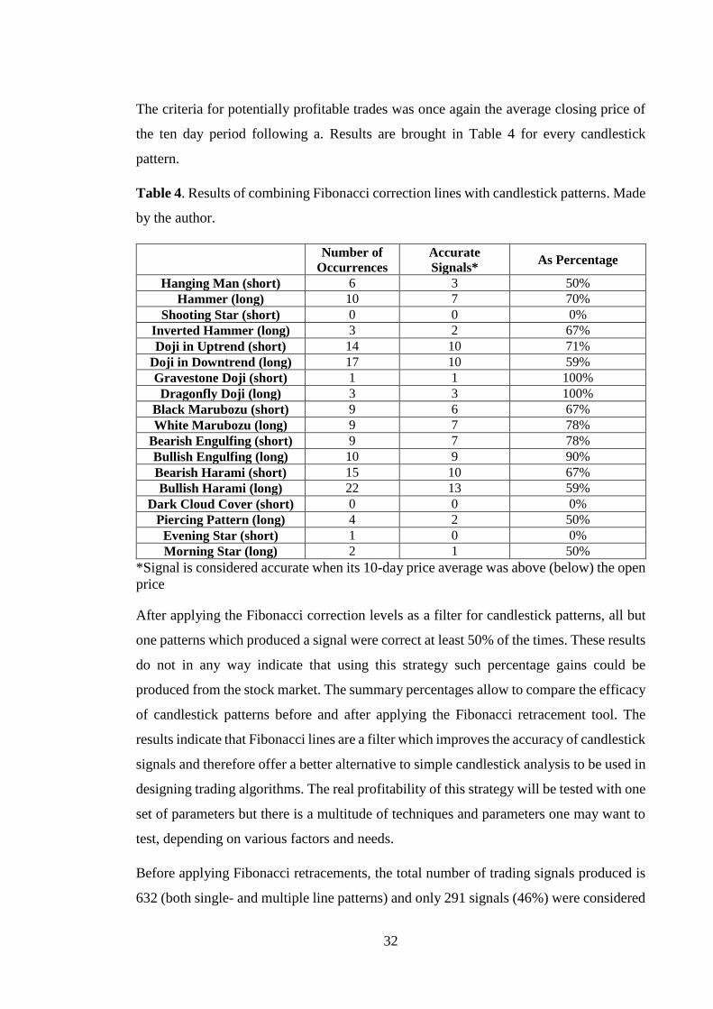
The criteria for potentially profitable trades was once again the average closing price of

the ten day period following a. Results are brought in Table 4 for every candlestick

pattern.

Table 4. Results of combining Fibonacci correction lines with candlestick patterns. Made

by the author.

Number of

Occurrences

Accurate

Signals* As Percentage

Hanging Man (short) 6 3 50%

Hammer (long) 10 7 70%

Shooting Star (short) 0 0 0%

Inverted Hammer (long) 3 2 67%

Doji in Uptrend (short) 14 10 71%

Doji in Downtrend (long) 17 10 59%

Gravestone Doji (short) 1 1 100%

Dragonfly Doji (long) 3 3 100%

Black Marubozu (short) 9 6 67%

White Marubozu (long) 9 7 78%

Bearish Engulfing (short) 9 7 78%

Bullish Engulfing (long) 10 9 90%

Bearish Harami (short) 15 10 67%

Bullish Harami (long) 22 13 59%

Dark Cloud Cover (short) 0 0 0%

Piercing Pattern (long) 4 2 50%

Evening Star (short) 1 0 0%

Morning Star (long) 2 1 50%

*Signal is considered accurate when its 10-day price average was above (below) the open

price

After applying the Fibonacci correction levels as a filter for candlestick patterns, all but

one patterns which produced a signal were correct at least 50% of the times. These results

do not in any way indicate that using this strategy such percentage gains could be

produced from the stock market. The summary percentages allow to compare the efficacy

of candlestick patterns before and after applying the Fibonacci retracement tool. The

results indicate that Fibonacci lines are a filter which improves the accuracy of candlestick

signals and therefore offer a better alternative to simple candlestick analysis to be used in

designing trading algorithms. The real profitability of this strategy will be tested with one

set of parameters but there is a multitude of techniques and parameters one may want to

test, depending on various factors and needs.

Before applying Fibonacci retracements, the total number of trading signals produced is

632 (both single- and multiple line patterns) and only 291 signals (46%) were considered

33

potentially profitable. It is clear that such a percentage does not indicate an efficient

investment strategy. After reducing the number of signals using Fibonacci filtering

system described above, the amount of signals dropped to 135 (slightly less than a quarter

of the unfiltered signals) and out of those 91 (67%) predicted the average price of the

following 10 days to be in the desired area. Considering all the candlestick patterns, both

single and multiple lines, the results have improved remarkably.

These findings confirm earlier research results from European markets that the Hanging

Man, Hammer and Engulfing pattern are all potentially profitable candlestick formations

but to achieve this profitability, Fibonacci retracement lines should be added to the mix.

At the same time the usefulness of candlestick patterns alone is refuted, confirming the

statistical findings from the US and Japanese equity markets by Marshall et al (2006 and

2008).

These results pave the way to construct any number of trading systems at the investor’s

desire, knowing that the combination of these two instruments yields better results than

candlestick patterns alone. However, this leaves the curious mind wanting, since no

examples have been provided on the possible applications of this knowledge. To find out

if this theory can be applied to the S&P 500 index to actually generate a profit. The

conditions of entering and exiting a position have already been described in previous

sections of the work: position gets closed (stopped out) with a loss of -3% and closed with

profit (reaches target) at +10%.

By applying a simple non-trailing stop-loss rule, a mere 34% of the trades were closed

with profits (i.e. were not stopped out with small losses). In total figures it means that 45

out of 134 trades resulted in positive earnings. Even though the rules for entering and

exiting the trade were same throughout the observed period, the individual amounts

gained or lost in a particular trade are quite different because of slippage7 (targets and

stop-losses calculated based on signal price data, see chapter 2.1) and growth/decline of

the index value itself. The greatest loss in absolute numbers occurred in January 2014

with a short-selling trade ($-91.48 or -5%) and greatest gain in June 2016 with a long

order ($233.03 or +12%). For the complete list of trades (order book) see Appendix 1.

7 The difference between expected price and actual price at which the trade is executed, here means the

gaps in price between signal candle closing price and next day opening price.

34

For further calculations and quantitative analysis the cumulative return of each

candlestick pattern is found by multiplying the S&P500 Index daily returns with either 1

or -1 (for short side trades) for every day that a position was held. This means creating a

vector in RStudio where the index return exists for every day that a position was open

and 0% return for every day that no positions existed. This allows equal treatment of the

S&P500 buy-hold strategy and use of that index as a benchmark index with which to

compare the Fibonacci candlesticks strategy. Cumulative returns are found using

arithmetic chaining to aggregate the returns which assumes equal position size for every

trade. The cumulative returns for the tested strategy are summarized in Table 5.

Table 5. Cumulative returns of the strategy (by pattern). Made by author

Bearish Candlestick

Patterns

Cumulative

Returns

Bullish Candlestick

Patterns

Cumulative

Returns

Bearish Engulfing

Pattern 27.78% Bullish Engulfing Pattern 46.59%

Black Marubozu 41.16% Bullish Harami 86.04%

Dark Cloud Cover 0.00% Dragonfly Doji 22.18%

Bearish Harami 27.78% Hammer 50.19%

Evening Star 0.00% Inverted Hammer 11.59%

Gravestone Doji 0.00% Morning Star 13.06%

Hanging Man 12.54% Piercing Pattern 11.4%

Shooting Star 0.00% Doji in Downtrend 74.17%

Doji in Uptrend 19.35% White Marubozu 57.11%

It appears that the most productive pattern in the strategy was Bullish Harami formation

which produced a return of 86% over the period under observation (roughly 8.6% a year).

The smallest returns were generated by the Piercing Pattern and Inverted Hammer, both

bringing in a rather modest 11% return for ten years. For the same period, the S&P 500

Index cumulative return was 82.3%, making the Bullish Harami also the only candlestick

pattern in the strategy which on its own could outperform the index. The cumulative

returns of bullish signals (buy signals) only was 372.33% and bearish (sell) signals

128.61% showing once again that buy signals were far more profitable in the context of

the data selection. For illustrative charts on the cumulative returns, drawdowns and daily

returns see Appendix 2 (for tested Fibonacci Candlestick strategy) and Appendix 3

(benchmark buy-hold strategy on S&P500 Index).

35

Figure 9. Q-Q plots of S&P500 returns (left) and strategy returns (right). Made by author

The Q-Q plots8 on figure 9 (index and strategy return quantiles plotted against normal

theoretical quantiles) show that the data is not following normal distribution and has

rather large values at either end of the quantile range. The presence of a high degree of

kurtosis (“fat tails”) is considered when calculating the risk-adjusted returns (VaR Sharpe

ratio is provided). The distributions of the returns are similar for both strategies, although

Index returns follow normal distribution closer.

The data about returns on investment, calculated daily for both S&P500 Index (also the

benchmark index for comparing strategies) and the Fibonacci Candlestick strategy allows

the calculation of various ratios which are used to evaluate the “goodness” of a given

portfolio. Those metrics are brought in table 6. Some of those ratios are representing the

same categories of assessment ratios (such as Sharpe and Sortino ratios) but are still

brought separate for the convenience of the reader, should one take more interest in a

slightly different ratio than used for the strategy assessment by the author.

The evaluation metrics in table 6 show that the composed strategy outperforms simple

buy and hold strategy in multiple categories. On average it takes the portfolio 5 days to

recover (achieve previous peak) after a drawdown whereas the buy-hold strategy requires

15 days for recovery. The size of the drawdowns is also more favorable for author’s

strategy as maximum portfolio drawdown was limited to less than 6% (thanks to stop-

loss rules) and for S&P500 the maximum drawdown was 66% (that due to the financial

crisis of 2008) although average drawdown is smaller for the Index returns.

Table 6. Portfolio evaluation metrics for Fibonacci Candlestick strategy (benchmark

S&P500 Index). Made by author.

METRIC STRATEGY VALUE BUY-HOLD VALUE

Average Recovery Period 4.7 14.9

8 Normal distribution quantiles are projected on the horizontal axis and return distribution on vertical axis.

36

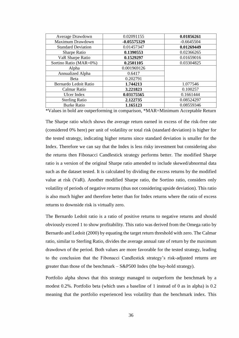
Average Drawdown 0.02091155 0.01856261

Maximum Drawdown -0.05575329 -0.6645504

Standard Deviation 0.01457347 0.01269449

Sharpe Ratio 0.1390553 0.02366265

VaR Sharpe Ratio 0.1529297 0.01659016

Sortino Ratio (MAR=0%) 0.2501105 0.03304825

Alpha 0.001969126

Annualized Alpha 0.6417

Beta 0.202791

Bernardo Ledoit Ratio 1.744213 1.077546

Calmar Ratio 3.221823 0.100257

Ulcer Index 0.03175565 0.1661444

Sterling Ratio 2.122735 0.08524297

Burke Ratio 1.165123 0.08559346

*Values in bold are outperforming in comparison, *MAR=Minimum Acceptable Return

The Sharpe ratio which shows the average return earned in excess of the risk-free rate

(considered 0% here) per unit of volatility or total risk (standard deviation) is higher for

the tested strategy, indicating higher returns since standard deviation is smaller for the

Index. Therefore we can say that the Index is less risky investment but considering also

the returns then Fibonacci Candlestick strategy performs better. The modified Sharpe

ratio is a version of the original Sharpe ratio amended to include skewed/abnormal data

such as the dataset tested. It is calculated by dividing the excess returns by the modified

value at risk (VaR). Another modified Sharpe ratio, the Sortino ratio, considers only

volatility of periods of negative returns (thus not considering upside deviation). This ratio

is also much higher and therefore better than for Index returns where the ratio of excess

returns to downside risk is virtually zero.

The Bernardo Ledoit ratio is a ratio of positive returns to negative returns and should

obviously exceed 1 to show profitability. This ratio was derived from the Omega ratio by

Bernardo and Ledoit (2000) by equating the target return threshold with zero. The Calmar

ratio, similar to Sterling Ratio, divides the average annual rate of return by the maximum

drawdown of the period. Both values are more favorable for the tested strategy, leading

to the conclusion that the Fibonacci Candlestick strategy’s risk-adjusted returns are

greater than those of the benchmark – S&P500 Index (the buy-hold strategy).

Portfolio alpha shows that this strategy managed to outperform the benchmark by a

modest 0.2%. Portfolio beta (which uses a baseline of 1 instead of 0 as in alpha) is 0.2

meaning that the portfolio experienced less volatility than the benchmark index. This

37

however is less reliable indicator in this context than for example standard deviation since

the portfolio’s R-squared value in relation to the benchmark is relatively low: 0.0332. It

means that only about 3% of the movements of the Fibonacci Candlestick strategy could

be explained by movements in the S&P500 index although the asset traded in both cases

is the same.

An interesting and intuitive way to assess the “goodness” of a strategy is also to consider

the probability an investor investing at any point in time will outperform the benchmark

over a given horizon. This method is more used in marketing and is rather a robust

estimate but nevertheless gives investor an idea at a glance how likely they are to

outperform the benchmark index. For the probabilities, see table 7.

It is evident that the longer the observed period is, the more likely is the strategy to

outperform its benchmark index. If the two strategies are compared during a period of

two months (or roughly 36 days considering possible holidays and other days when

markets are closed) then the Fibonacci Candlestick strategy will with over 70% likelihood

outperform the buy-hold strategy based on the S&P500 daily returns.

Table 7. Probabilities that the Fibonacci Candlestick strategy will outperform benchmark.

Periods in days. Made by author.

Periods Strategy outperforming

benchmark (S&P500)

1 0.5215356

3 0.5467958

6 0.5807327

9 0.6037317

12 0.6209007

18 0.6432225

36 0.7183442

To summarize the results, adding Fibonacci retracement lines to candlestick patterns

helps to improve the accuracy of those signals. Testing the Fibonacci and candlestick

pattern combination strategy gave better results in both risk and return categories than

buy and hold strategy of the same asset. These results can be generalized for equity

markets in the U.S. considering the proposed descriptiveness of the S&P500 Index for

the American stock market in general. However, the profitability of the strategy with -3%

stop-loss and +10% profit target proves weak, considering the systemic risk involved in

38

the trading algorithm. The total cumulative return of the strategy adds to 517.16% over

ten years, meaning on average about 51.7% a year. Averaging this return to the number

of candlestick patterns (18) gives a return per pattern of 2.9% a year or 3.7% when

calculated over signal producing candlesticks (14). Many investors may consider this

return too low, especially considering that the risk-adjusted return for the portfolio

(Sharpe ratio) was 0.14, far smaller value than 1 which is usually the minimum value

recommended for investing (Maverick, 2018). The profitability of the strategy as a whole

can be improved by excluding less profitable candlestick formations from the mix and

relying only on few most profitable ones. It is also possible to improve results by adjusting

the price target and stop-loss rules. This research has proved that Fibonacci retracements

offer added value to candlestick analysis and shows by example how profitable one such

strategy could be. Author urges all readers to understand that past performance does not

guarantee future results but it seems that at very least past performance can offer better

insight and increase chances of success.

39

CONCLUSIONS

This research studied ten years of S&P 500 index price data to find whether candlestick

analysis in conjunction with Fibonacci retracement levels can predict price movements

and be therefore applied as a trading strategy. The theoretical part of this research covers

the formation of candlestick patterns and their use in price predictions as well as the use

of Fibonacci retracement lines and its connection to general market patterns, specifically

the Elliott wave theory. Empirical analysis used both theoretical and practical testing of

the trading methodology.

It was noted that the literature concerning technical trading rules (such as the indicators

tested in this work) was mainly written by practitioners and analysts who execute trades

on their clients’ accounts as a day job. Academic literature about technical analysis is

readily available in some categories (like for candlestick analysis) but lacks in other

categories (Fibonacci trading tools). Researchers have pointed out that the reason why

literature and trading results by active traders and investors is more favoring technical

analysis may be the presence of tacit knowledge accumulated over years of practice that

can improve the overall performance of the trader. This means that it is possible that

technical analysis is profitable thanks to other factors that are tacit and are not

transferrable knowledge. It is supported also by the fact that most articles on technical

analysis return the conclusion that the indicator under observation did not yield any

significant gains.

It is evident that there is no consensus on how strong predictive power Fibonacci

retracements have and which of them are more “respected” by the market. Academics

have obtained somewhat conflicting results with different research methods, latest papers

reveal that none of the retracement values have significant advantage over another.

Practitioners seem to have opinions on which lines are more predictive, their opinions are

40

often conflicting and there is no clarity in how exactly are those opinions formed or on

what research are they based.

Candlestick analysis is more clearly formulated than Fibonacci analysis and has less room

for interpretation. The main problem with candlestick analysis is the subjectivity of the

trader and his or her tacit knowledge. Candlestick signals are visual prediction tools and

therefore have a higher degree of freedom in interpretation than for example Fibonacci

retracements which are defined as fixed percentages. Scientific research has been

extensively carried out for candlestick signals, results depend on the financial markets

and research methods.

The empirical part of this research first determined the potential profitability of

candlestick analysis as an individual strategy and then in combination with Fibonacci

retracement lines. In the end, a computational example is provided about the efficacy of

the strategy using stop-loss rule and price targets.

The key findings are the following:

Out of 18 candlestick patterns examined, only 10 showed profit potential when

used alone;

When Fibonacci retracement lines were added, 12 out of 16 patterns turned out to

be potentially profitable (two patterns yielded no signals);

Bullish patterns perform better than their bearish counterparts;

Doji candles at Fibonacci levels are profitable signals but they perform better in

downtrend than uptrend;

Total cumulative returns for the strategy are 517.16%, making an average yearly

return for a candlestick pattern 3.7% (excluding patterns with no signals);

Sharpe ratio for risk-adjusted returns is greater for the integrated strategy than for

buy-hold strategy but both of those values are smaller than 1;

Buy-hold strategy did not outperform the tested strategy in any risk-return

evaluation category apart the size of average drawdown and standard deviation of

the returns.

All of the Fibonacci retracement levels, including the 50% level were treated equally and

no testing was conducted regarding the reliability of any retracement in particular. The

41

retracements were located using a ZigZag tool to smooth the price data (with 2.5%

sensitivity) for finding relevant peaks and valleys in the data. Trend was determined by

using 20 period Donchian channel with 1/3 division – upper third meaning uptrend, lower

third downtrend and middle third indicates the absence of a trend. The profitability of

trading signals was assessed using 10 day average closing price following a signal.

According to the conducted research, there is positive potential in using Fibonacci

retracements and candlestick patterns simultaneously for predicting equity market price

movements. Since the sample dataset is descriptive of the U.S. equity market then further

research is needed to confirm or refute the efficacy of this strategy in other markets,

including FOREX and commodities markets.

In addition, this research is limited to proving that Fibonacci retracements as a filter

increase the accuracy of candlestick pattern signals. The results obtained assist investors

in choosing the most profitable candlestick formations for predicting future price

movements and prove the efficacy of adding Fibonacci analysis to candlestick analysis.

An example of the efficacy of the system is shown using certain stop-loss and price target

rules but since different investors have different trading styles, rules and guidelines then

it serves as just one of many possible ways of applying the strategy. Further research is

needed to check whether these results are consistent in other markets and offer similar

efficacy when applied to separate stocks and commodities. Testing with different levels

of risk (stop-loss rules) would also provide greater understanding about the profitability

of the system.

42

REFERENCES

1. Baranauskas, S. (2011). Elliott wave and Fibonacci level mutual relationship and

applying in a stock market. Business: theory and practice. Vol. 12 (4), pp 390-397

2. Bhattacharya, S., Kumar, K. (2006). A computational exploration of the

efficacy of Fibonacci Sequences in Technical analysis and trading. Bond Business

School Publications.

3. Bernardo, A., Ledoit, O. (2000). "Gain, Loss, and Asset Pricing". Journal of

Political Economy. 108 (1): 144–172.

4. Boroden, C. (2008). Fibonacci Trading: How to Master the Time and Price

Advantage. McGraw-Hill. 303pp

5. Bulkowski, T. (2005). Encyclopedia of Chart Patterns, 2nd edition, Wiley

Trading, 1035 pp.

6. Chen, S., Bao, S., Zhou, Y. (2016). The predictive power of Japanese candlestick

charting in Chinese stock market. Physica A. Statistical Mechanics and its

Applications. Vol. 457, pp 148-165

7. Erman, W. (1999). Log Spirals on the Markets and In Nature. Technical Analysis

of Common Stocks & Commodities, vol. 17 (2) pp 16:34

8. Fischer, R., Fischer, J. (2003). Candlesticks, Fibonacci, and Chart Pattern

Trading Tools: A Synergistic Strategy to Enhance Profits and Reduce Risk. John

Wiley and Sons, pp 256.

9. Gaucan, V. (2010). How to Use Fibonacci Retracement to Predict Forex Market.

Titu Maiorescu University, Bucharest, Romania. Journal of Knowledge

Management, Economics and Information Technology. Vol. 1 Issue 2.

10. Greenblatt, J. (2007). Trading Stocks with Fibonacci and Lucas.

[http://www.futuresmag.com/2007/04/18/trading-stocks-fibonacci-and-lucas]

11. Hartle, T. (1997). Fibonacci Trader Product Review – Stock & Commodities

Magazine, pp 1-15.

43

12. Joseph, T. (1999). Applying Technical Analysis. Trading Techniques, Inc. pp182

13. Krausz, R. (1998). New Gann Swing Charist Dynamic Fibonacci Channels. –

Fibonacci Trader Journal, Vol. 1, No. 1: 1-8.

14. Lien, K. (2004). Basic Guide to Understanding Elliott Wave. Daily FX Research.

pp6

15. Linton, D. (2010). Cloud Charts: Trading success with the Ichimoku technique.

Updata Plc, London. Pp 240

16. Kempen, R. (2016). Fibonaccis Are Human (Made). IFTA Journal. 2016 Edition.

The International Federation of Technical Analysts. Pp 77

17. Maiani, G. (2002). How Reliable Are Candlesticks? Technical Analysis of Stocks

& Commodities, pp. 60–65.

18. Michalowski, G. (2012). Trading Forex with the Trend.

[http://www.futuresmag.com/2012/08/31/trading-forex-trend]

19. Marshall, B.R., Young, M.R. & Cahan, R. Rev Quant Finan Acc (2008) 31:

191. https://doi.org/10.1007/s11156-007-0068-1

20. Marshall, B. R., Young, M. R., Rose, L. C. (2006). Candlestick technical trading

strategies: Can they create value for investors? Journal of Banking & Finance 30,

pp 2303–2323.

21. Mayall, M. (2006). Seeing the market: Technical analysis in trading styles.

Journal for the Theory of Social Behaviour, 36 (2), pp 119–140.

22. Maverick, J.B. What is a good Sharpe ratio? Investopedia.

[https://www.investopedia.com/ask/answers/010815/what-good-sharpe-

ratio.asp] 11.01.2018

23. Morris, G. L. (2006). Candlestick Charting Explained: Timeless Techniques for

Trading Stocks and Futures. McGraw-Hill. Pp 560

24. Nison, S. (1994). Beyond Candlesticks: New Japanese Charting Techniques

Revealed. Wiley Finance

25. Nison, S. (1991). Japanese Candlestick Charting Techniques: A Contemporary

Guide to the Ancient Investment. New York Institute of Finance Simon &

Schuster. Pp 315

26. Nison, S. (2003). The Candlestick Course. John Wiley and Sons, pp 219

44

27. O’Neil, W.J. (1988). How to Make Money in Stocks. New York, McGraw-Hill,

pp 464.

28. Prechter, R. R. Jr., Frost, A. J. (2005). Elliott wave principle: Key to Market

Behavior. 10th edition. New Classics Library. Pp 255.

29. Prechter, R. R. Jr. (2005). Elliott Waves, Fibonacci and Statistics.

[http://www.socionomics.org/pdf/EW_Fibo_Statistics.pdf]

30. Roscoe, P., Howorth, C. (2009). Identification through technical analysis: A

study of charting and UK non-professional investors. Accounting, Organizations

and Society, vol. 34 pp. 206-221

31. Schlossberg, B. (2006). Technical analysis of the currency market: classic

techniques for profiting from market swings and trader sentiment. John Wiley &

Sons. Pp 225

32. Teweles, R.J., F.J. Jones, and B. Warwick. (1987). The Futures Game: Who

Wins? Who Loses? Why? New York, McGraw-Hill, pp 279.

33. Wagner, G. S. (2010). Gold and the New Technical Triad. Stocks &

Commodities V. 28:8 (12-17)

34. Williams, B. (2012). It’s Not Witchcraft, it’s Fibonacci. Futures Magazine.

[http://www.futuresmag.com/2012/05/29/it%E2%80%99s-not-witchcraft-

it%E2%80%99s-fibonacci]

45

APPENDIXES

Appendix 1. Order book. Made by author, based on Yahoo Finance data.

Open date

(D.MM.YYYY)

Order

Side

Open

price

Price

Target

Stop-loss

order

Close date

(D.MM.YYYY)

Close

price

Profit or

Loss

Profit or

Loss

(%)

Duration

(days)

7.03.2007 LONG $1 395,02 $ 1 534,95 $ 1 353,55 31.05.2007 $1 534,95 $ 139,93 10,03% 85

9.03.2007 LONG $1 401,89 $ 1 542,08 $ 1 359,83 13.07.2007 $1 542,08 $ 140,19 10,00% 126

2.08.2007 LONG $1 465,46 $ 1 612,39 $ 1 421,84 15.08.2007 $1 421,84 $ -43,62 -2,98% 13

7.08.2007 LONG $1 467,62 $ 1 614,44 $ 1 423,64 15.08.2007 $1 423,64 $ -43,98 -3,00% 8

10.08.2007 SHORT $1 453,09 $ 1 307,78 $ 1 542,13 1.10.2007 $1 542,13 $ -89,04 -6,13% 52

13.08.2007 LONG $1 453,42 $ 1 599,00 $ 1 410,03 15.08.2007 $1 410,03 $ -43,39 -2,99% 2

17.08.2007 LONG $1 411,26 $ 1 552,40 $ 1 368,93 5.10.2007 $1 552,40 $ 141,14 10,00% 49

28.08.2007 SHORT $1 466,72 $ 1 320,11 $ 1 523,74 19.09.2007 $1 523,74 $ -57,02 -3,89% 22

30.08.2007 LONG $1 463,67 $ 1 610,14 $ 1 419,85 21.11.2007 $1 419,85 $ -43,82 -2,99% 83

16.10.2007 SHORT $1 547,81 $ 1 393,84 $ 1 611,68 8.01.2008 $1 393,84 $ 153,97 9,95% 84

25.10.2007 LONG $1 516,15 $ 1 667,47 $ 1 470,40 8.11.2007 $1 470,40 $ -45,75 -3,02% 14

25.10.2007 LONG $1 516,15 $ 1 667,47 $ 1 470,40 8.11.2007 $1 470,40 $ -45,75 -3,02% 14

26.10.2007 LONG $1 522,17 $ 1 665,84 $ 1 468,97 8.11.2007 $1 468,97 $ -53,20 -3,50% 13

28.11.2007 LONG $1 432,95 $ 1 571,05 $ 1 385,38 9.01.2008 $1 385,38 $ -47,57 -3,32% 42

13.12.2007 SHORT $1 483,27 $ 1 337,93 $ 1 557,32 17.01.2008 $1 337,93 $ 145,34 9,80% 35

10.01.2008 LONG $1 406,78 $ 1 550,04 $ 1 366,86 16.01.2008 $1 366,86 $ -39,92 -2,84% 6

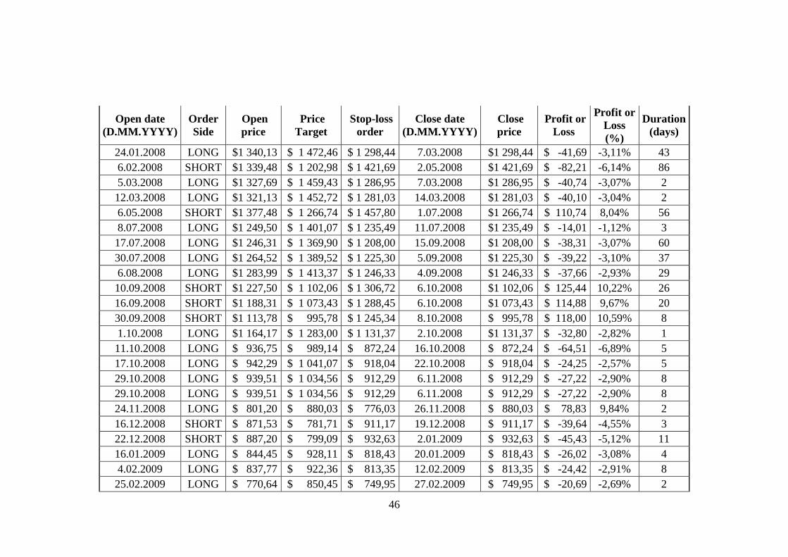
46

Open date

(D.MM.YYYY)

Order

Side

Open

price

Price

Target

Stop-loss

order

Close date

(D.MM.YYYY)

Close

price

Profit or

Loss

Profit or

Loss

(%)

Duration

(days)

24.01.2008 LONG $1 340,13 $ 1 472,46 $ 1 298,44 7.03.2008 $1 298,44 $ -41,69 -3,11% 43

6.02.2008 SHORT $1 339,48 $ 1 202,98 $ 1 421,69 2.05.2008 $1 421,69 $ -82,21 -6,14% 86

5.03.2008 LONG $1 327,69 $ 1 459,43 $ 1 286,95 7.03.2008 $1 286,95 $ -40,74 -3,07% 2

12.03.2008 LONG $1 321,13 $ 1 452,72 $ 1 281,03 14.03.2008 $1 281,03 $ -40,10 -3,04% 2

6.05.2008 SHORT $1 377,48 $ 1 266,74 $ 1 457,80 1.07.2008 $1 266,74 $ 110,74 8,04% 56

8.07.2008 LONG $1 249,50 $ 1 401,07 $ 1 235,49 11.07.2008 $1 235,49 $ -14,01 -1,12% 3

17.07.2008 LONG $1 246,31 $ 1 369,90 $ 1 208,00 15.09.2008 $1 208,00 $ -38,31 -3,07% 60

30.07.2008 LONG $1 264,52 $ 1 389,52 $ 1 225,30 5.09.2008 $1 225,30 $ -39,22 -3,10% 37

6.08.2008 LONG $1 283,99 $ 1 413,37 $ 1 246,33 4.09.2008 $1 246,33 $ -37,66 -2,93% 29

10.09.2008 SHORT $1 227,50 $ 1 102,06 $ 1 306,72 6.10.2008 $1 102,06 $ 125,44 10,22% 26

16.09.2008 SHORT $1 188,31 $ 1 073,43 $ 1 288,45 6.10.2008 $1 073,43 $ 114,88 9,67% 20

30.09.2008 SHORT $1 113,78 $ 995,78 $ 1 245,34 8.10.2008 $ 995,78 $ 118,00 10,59% 8

1.10.2008 LONG $1 164,17 $ 1 283,00 $ 1 131,37 2.10.2008 $1 131,37 $ -32,80 -2,82% 1

11.10.2008 LONG $ 936,75 $ 989,14 $ 872,24 16.10.2008 $ 872,24 $ -64,51 -6,89% 5

17.10.2008 LONG $ 942,29 $ 1 041,07 $ 918,04 22.10.2008 $ 918,04 $ -24,25 -2,57% 5

29.10.2008 LONG $ 939,51 $ 1 034,56 $ 912,29 6.11.2008 $ 912,29 $ -27,22 -2,90% 8

29.10.2008 LONG $ 939,51 $ 1 034,56 $ 912,29 6.11.2008 $ 912,29 $ -27,22 -2,90% 8

24.11.2008 LONG $ 801,20 $ 880,03 $ 776,03 26.11.2008 $ 880,03 $ 78,83 9,84% 2

16.12.2008 SHORT $ 871,53 $ 781,71 $ 911,17 19.12.2008 $ 911,17 $ -39,64 -4,55% 3

22.12.2008 SHORT $ 887,20 $ 799,09 $ 932,63 2.01.2009 $ 932,63 $ -45,43 -5,12% 11

16.01.2009 LONG $ 844,45 $ 928,11 $ 818,43 20.01.2009 $ 818,43 $ -26,02 -3,08% 4

4.02.2009 LONG $ 837,77 $ 922,36 $ 813,35 12.02.2009 $ 813,35 $ -24,42 -2,91% 8

25.02.2009 LONG $ 770,64 $ 850,45 $ 749,95 27.02.2009 $ 749,95 $ -20,69 -2,69% 2

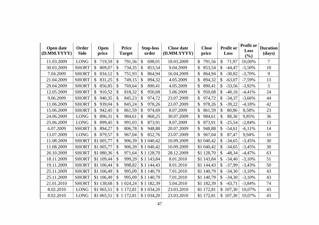
47

Open date

(D.MM.YYYY)

Order

Side

Open

price

Price

Target

Stop-loss

order

Close date

(D.MM.YYYY)

Close

price

Profit or

Loss

Profit or

Loss

(%)

Duration

(days)

11.03.2009 LONG $ 719,59 $ 791,56 $ 698,01 18.03.2009 $ 791,56 $ 71,97 10,00% 7

30.03.2009 SHORT $ 809,07 $ 734,35 $ 853,54 9.04.2009 $ 853,54 $ -44,47 -5,50% 10

7.04.2009 SHORT $ 834,12 $ 751,93 $ 864,94 16.04.2009 $ 864,94 $ -30,82 -3,70% 9

21.04.2009 SHORT $ 831,25 $ 749,15 $ 894,32 4.05.2009 $ 894,32 $ -63,07 -7,59% 13

29.04.2009 SHORT $ 856,85 $ 769,64 $ 890,41 4.05.2009 $ 890,41 $ -33,56 -3,92% 5

12.05.2009 SHORT $ 910,52 $ 818,32 $ 950,68 5.06.2009 $ 950,68 $ -40,16 -4,41% 24

9.06.2009 SHORT $ 940,35 $ 845,23 $ 974,72 23.07.2009 $ 974,72 $ -34,37 -3,66% 44

11.06.2009 SHORT $ 939,04 $ 845,24 $ 978,26 23.07.2009 $ 978,26 $ -39,22 -4,18% 42

15.06.2009 SHORT $ 942,45 $ 861,59 $ 974,69 8.07.2009 $ 861,59 $ 80,86 8,58% 23

24.06.2009 LONG $ 896,31 $ 984,61 $ 868,25 30.07.2009 $ 984,61 $ 88,30 9,85% 36

25.06.2009 LONG $ 899,45 $ 991,03 $ 873,91 8.07.2009 $ 873,91 $ -25,54 -2,84% 13

6.07.2009 SHORT $ 894,27 $ 806,78 $ 948,88 20.07.2009 $ 948,88 $ -54,61 -6,11% 14

13.07.2009 LONG $ 879,57 $ 967,04 $ 852,76 23.07.2009 $ 967,04 $ 87,47 9,94% 10

11.08.2009 SHORT $1 005,77 $ 906,39 $ 1 040,42 10.09.2009 $1 040,42 $ -34,65 -3,45% 30

11.08.2009 SHORT $1 005,77 $ 906,39 $ 1 040,42 10.09.2009 $1 040,42 $ -34,65 -3,45% 30

26.10.2009 SHORT $1 080,36 $ 971,64 $ 1 128,70 28.12.2009 $1 128,70 $ -48,34 -4,47% 63

18.11.2009 SHORT $1 109,44 $ 999,29 $ 1 143,84 8.01.2010 $1 143,84 $ -34,40 -3,10% 51

19.11.2009 SHORT $1 106,44 $ 998,82 $ 1 144,43 8.01.2010 $1 144,43 $ -37,99 -3,43% 50

25.11.2009 SHORT $1 106,49 $ 995,09 $ 1 140,79 7.01.2010 $1 140,79 $ -34,30 -3,10% 43

25.11.2009 SHORT $1 106,49 $ 995,09 $ 1 140,79 7.01.2010 $1 140,79 $ -34,30 -3,10% 43

21.01.2010 SHORT $1 138,68 $ 1 024,24 $ 1 182,39 5.04.2010 $1 182,39 $ -43,71 -3,84% 74

8.02.2010 LONG $1 065,51 $ 1 172,81 $ 1 034,20 23.03.2010 $1 172,81 $ 107,30 10,07% 43

8.02.2010 LONG $1 065,51 $ 1 172,81 $ 1 034,20 23.03.2010 $1 172,81 $ 107,30 10,07% 43

48

Open date

(D.MM.YYYY)

Order

Side

Open

price

Price

Target

Stop-loss

order

Close date

(D.MM.YYYY)

Close

price

Profit or

Loss

Profit or

Loss

(%)

Duration

(days)

8.02.2010 LONG $1 065,51 $ 1 172,81 $ 1 034,20 23.03.2010 $1 172,81 $ 107,30 10,07% 43

26.05.2010 LONG $1 075,51 $ 1 181,43 $ 1 041,81 30.06.2010 $1 041,81 $ -33,70 -3,13% 35

9.06.2010 LONG $1 062,75 $ 1 168,20 $ 1 030,14 30.06.2010 $1 030,14 $ -32,61 -3,07% 21

7.07.2010 LONG $1 028,54 $ 1 130,87 $ 997,22 17.09.2010 $1 130,87 $ 102,33 9,95% 72

15.07.2010 SHORT $1 094,46 $ 985,65 $ 1 132,05 20.09.2010 $1 132,05 $ -37,59 -3,43% 67

16.07.2010 SHORT $1 093,85 $ 986,83 $ 1 131,62 20.09.2010 $1 131,62 $ -37,77 -3,45% 66

10.11.2010 SHORT $1 213,14 $ 1 092,06 $ 1 263,65 3.01.2011 $1 263,65 $ -50,51 -4,16% 54

30.11.2010 LONG $1 182,96 $ 1 306,54 $ 1 152,13 1.02.2011 $1 306,54 $ 123,58 10,45% 63

30.11.2010 LONG $1 182,96 $ 1 306,54 $ 1 152,13 1.02.2011 $1 306,54 $ 123,58 10,45% 63

18.03.2011 LONG $1 276,71 $ 1 401,09 $ 1 235,51 3.08.2011 $1 235,51 $ -41,20 -3,23% 138

20.06.2011 LONG $1 271,50 $ 1 398,65 $ 1 233,36 4.08.2011 $1 233,36 $ -38,15 -3,00% 45

24.06.2011 LONG $1 283,04 $ 1 411,85 $ 1 245,00 3.08.2011 $1 245,00 $ -38,05 -2,97% 40

28.06.2011 LONG $1 280,21 $ 1 408,11 $ 1 241,70 3.08.2011 $1 241,70 $ -38,51 -3,01% 36

11.07.2011 SHORT $1 343,31 $ 1 209,42 $ 1 392,96 4.08.2011 $1 209,42 $ 133,89 9,97% 24

10.08.2011 LONG $1 171,77 $ 1 289,78 $ 1 137,35 11.08.2011 $1 137,35 $ -34,42 -2,94% 1

23.08.2011 LONG $1 124,36 $ 1 236,20 $ 1 090,11 4.10.2011 $1 090,11 $ -34,25 -3,05% 42

23.08.2011 LONG $1 124,36 $ 1 236,20 $ 1 090,11 4.10.2011 $1 090,11 $ -34,25 -3,05% 42

5.10.2011 LONG $1 124,03 $ 1 236,34 $ 1 090,23 21.10.2011 $1 236,34 $ 112,31 9,99% 16

26.10.2011 SHORT $1 229,17 $ 1 106,15 $ 1 291,82 27.10.2011 $1 291,82 $ -62,65 -5,10% 1

29.11.2011 LONG $1 192,56 $ 1 311,81 $ 1 156,77 19.01.2012 $1 311,81 $ 119,24 10,00% 51

29.11.2011 LONG $1 192,56 $ 1 311,81 $ 1 156,77 19.01.2012 $1 311,81 $ 119,24 10,00% 51

13.12.2011 SHORT $1 236,83 $ 1 112,82 $ 1 292,70 10.01.2012 $1 292,70 $ -55,87 -4,52% 28

4.04.2012 SHORT $1 413,09 $ 1 274,16 $ 1 461,57 5.06.2012 $1 274,16 $ 138,93 9,83% 62

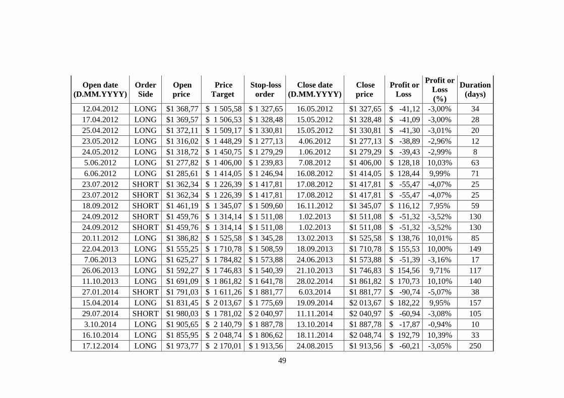
49

Open date

(D.MM.YYYY)

Order

Side

Open

price

Price

Target

Stop-loss

order

Close date

(D.MM.YYYY)

Close

price

Profit or

Loss

Profit or

Loss

(%)

Duration

(days)

12.04.2012 LONG $1 368,77 $ 1 505,58 $ 1 327,65 16.05.2012 $1 327,65 $ -41,12 -3,00% 34

17.04.2012 LONG $1 369,57 $ 1 506,53 $ 1 328,48 15.05.2012 $1 328,48 $ -41,09 -3,00% 28

25.04.2012 LONG $1 372,11 $ 1 509,17 $ 1 330,81 15.05.2012 $1 330,81 $ -41,30 -3,01% 20

23.05.2012 LONG $1 316,02 $ 1 448,29 $ 1 277,13 4.06.2012 $1 277,13 $ -38,89 -2,96% 12

24.05.2012 LONG $1 318,72 $ 1 450,75 $ 1 279,29 1.06.2012 $1 279,29 $ -39,43 -2,99% 8

5.06.2012 LONG $1 277,82 $ 1 406,00 $ 1 239,83 7.08.2012 $1 406,00 $ 128,18 10,03% 63

6.06.2012 LONG $1 285,61 $ 1 414,05 $ 1 246,94 16.08.2012 $1 414,05 $ 128,44 9,99% 71

23.07.2012 SHORT $1 362,34 $ 1 226,39 $ 1 417,81 17.08.2012 $1 417,81 $ -55,47 -4,07% 25

23.07.2012 SHORT $1 362,34 $ 1 226,39 $ 1 417,81 17.08.2012 $1 417,81 $ -55,47 -4,07% 25

18.09.2012 SHORT $1 461,19 $ 1 345,07 $ 1 509,60 16.11.2012 $1 345,07 $ 116,12 7,95% 59

24.09.2012 SHORT $1 459,76 $ 1 314,14 $ 1 511,08 1.02.2013 $1 511,08 $ -51,32 -3,52% 130

24.09.2012 SHORT $1 459,76 $ 1 314,14 $ 1 511,08 1.02.2013 $1 511,08 $ -51,32 -3,52% 130

20.11.2012 LONG $1 386,82 $ 1 525,58 $ 1 345,28 13.02.2013 $1 525,58 $ 138,76 10,01% 85

22.04.2013 LONG $1 555,25 $ 1 710,78 $ 1 508,59 18.09.2013 $1 710,78 $ 155,53 10,00% 149

7.06.2013 LONG $1 625,27 $ 1 784,82 $ 1 573,88 24.06.2013 $1 573,88 $ -51,39 -3,16% 17

26.06.2013 LONG $1 592,27 $ 1 746,83 $ 1 540,39 21.10.2013 $1 746,83 $ 154,56 9,71% 117

11.10.2013 LONG $1 691,09 $ 1 861,82 $ 1 641,78 28.02.2014 $1 861,82 $ 170,73 10,10% 140

27.01.2014 SHORT $1 791,03 $ 1 611,26 $ 1 881,77 6.03.2014 $1 881,77 $ -90,74 -5,07% 38

15.04.2014 LONG $1 831,45 $ 2 013,67 $ 1 775,69 19.09.2014 $2 013,67 $ 182,22 9,95% 157

29.07.2014 SHORT $1 980,03 $ 1 781,02 $ 2 040,97 11.11.2014 $2 040,97 $ -60,94 -3,08% 105

3.10.2014 LONG $1 905,65 $ 2 140,79 $ 1 887,78 13.10.2014 $1 887,78 $ -17,87 -0,94% 10

16.10.2014 LONG $1 855,95 $ 2 048,74 $ 1 806,62 18.11.2014 $2 048,74 $ 192,79 10,39% 33

17.12.2014 LONG $1 973,77 $ 2 170,01 $ 1 913,56 24.08.2015 $1 913,56 $ -60,21 -3,05% 250

50

Open date

(D.MM.YYYY)

Order

Side

Open

price

Price

Target

Stop-loss

order

Close date

(D.MM.YYYY)

Close

price

Profit or

Loss

Profit or

Loss

(%)

Duration

(days)

5.01.2015 SHORT $2 054,44 $ 1 852,38 $ 2 134,53 20.05.2015 $2 134,53 $ -80,09 -3,90% 135

4.03.2015 SHORT $2 107,72 $ 1 897,00 $ 2 179,23 24.08.2015 $1 897,00 $ 210,72 10,00% 173

30.03.2015 LONG $2 064,11 $ 2 267,12 $ 1 999,19 21.08.2015 $1 999,19 $ -64,92 -3,15% 144

29.05.2015 SHORT $2 120,66 $ 1 908,71 $ 2 185,94 24.08.2015 $1 908,71 $ 211,95 9,99% 87

29.05.2015 SHORT $2 120,66 $ 1 908,71 $ 2 185,94 24.08.2015 $1 908,71 $ 211,95 9,99% 87

10.06.2015 LONG $2 081,12 $ 2 288,16 $ 2 017,75 21.08.2015 $2 017,75 $ -63,37 -3,05% 72

10.07.2015 LONG $2 052,74 $ 2 256,44 $ 1 989,77 21.08.2015 $1 989,77 $ -62,97 -3,07% 42

10.07.2015 LONG $2 052,74 $ 2 256,44 $ 1 989,77 21.08.2015 $1 989,77 $ -62,97 -3,07% 42

13.08.2015 LONG $2 086,19 $ 2 294,66 $ 2 023,47 21.08.2015 $2 023,47 $ -62,72 -3,01% 8

21.08.2015 SHORT $2 034,08 $ 1 832,16 $ 2 138,91 20.01.2016 $1 832,16 $ 201,92 9,93% 152

3.09.2015 LONG $1 950,79 $ 2 143,75 $ 1 890,39 28.09.2015 $1 890,39 $ -60,40 -3,10% 25

6.11.2015 SHORT $2 098,60 $ 1 889,94 $ 2 172,04 15.01.2016 $1 889,94 $ 208,66 9,94% 70

9.11.2015 SHORT $2 096,56 $ 1 889,28 $ 2 164,97 15.01.2016 $1 889,28 $ 207,28 9,89% 67

8.12.2015 SHORT $2 073,39 $ 1 869,36 $ 2 153,13 15.01.2016 $1 869,36 $ 204,03 9,84% 38

15.12.2015 LONG $2 025,55 $ 2 224,13 $ 1 961,28 7.01.2016 $1 961,28 $ -64,27 -3,17% 23

15.12.2015 LONG $2 025,55 $ 2 224,13 $ 1 961,28 7.01.2016 $1 961,28 $ -64,27 -3,17% 23

22.12.2015 LONG $2 069,28 $ 2 223,27 $ 1 960,52 7.01.2016 $1 960,52 $ -108,76 -5,26% 16

21.01.2016 LONG $1 861,46 $ 2 045,26 $ 1 803,55 17.03.2016 $2 045,26 $ 183,80 9,87% 56

22.01.2016 LONG $1 877,40 $ 2 055,89 $ 1 812,92 11.02.2016 $1 812,92 $ -64,48 -3,43% 20

25.04.2016 SHORT $2 089,37 $ 1 882,42 $ 2 157,15 14.07.2016 $2 157,15 $ -67,78 -3,24% 80

20.05.2016 LONG $2 041,88 $ 2 244,04 $ 1 978,84 8.12.2016 $2 244,04 $ 202,16 9,90% 202

29.06.2016 LONG $2 042,69 $ 2 239,70 $ 1 975,01 7.12.2016 $2 239,70 $ 197,01 9,64% 161

22.08.2016 SHORT $2 181,58 $ 1 965,48 $ 2 250,55 8.12.2016 $2 250,55 $ -68,97 -3,16% 108

51

Open date

(D.MM.YYYY)

Order

Side

Open

price

Price

Target

Stop-loss

order

Close date

(D.MM.YYYY)

Close

price

Profit or

Loss

Profit or

Loss

(%)

Duration

(days)

22.08.2016 SHORT $2 181,58 $ 1 965,48 $ 2 250,55 8.12.2016 $2 250,55 $ -68,97 -3,16% 108

15.09.2016 LONG $2 125,36 $ 2 338,35 $ 2 062,00 15.02.2017 $2 338,35 $ 212,99 10,02% 153

3.03.2017 SHORT $2 380,92 $ 2 143,73 $ 2 466,59 19.07.2017 $2 466,59 $ -85,67 -3,60% 138

52

Appendix 2. Strategy performance summary. Made by author.

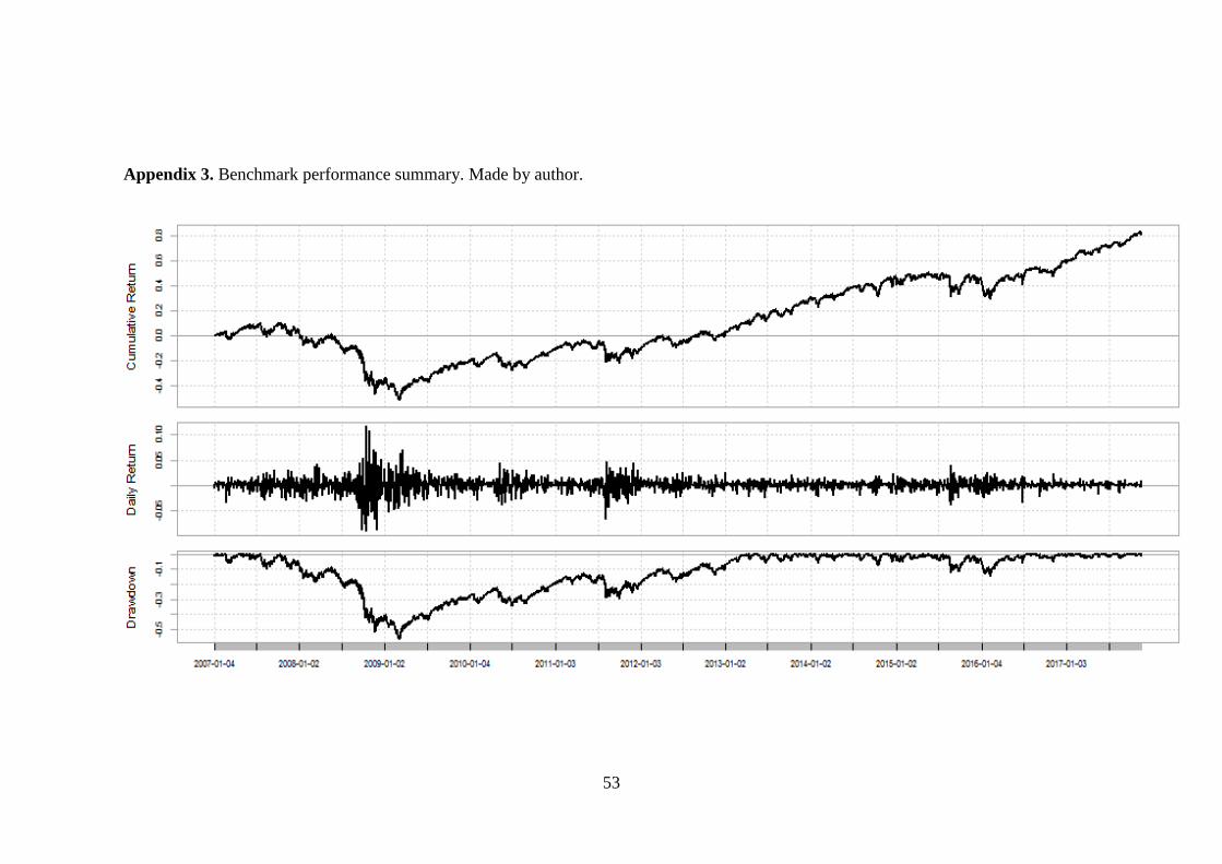
53

Appendix 3. Benchmark performance summary. Made by author.

54

KOKKUVÕTE

TRENDIKAUPLEMINE JAAPANI KÜÜNALMUSTREID JA FIBONACCI

KORREKTSIOONITASEMEID KOMBINEERIDES S&P500 INDEKSI NÄITEL

Martin Promen

Algoritmkauplemise ja küllusliku informatsiooni ajastul kasutavad pangad ja

investeerimisfondid keerukaid programme ja võimsaid arvuteid ennustamaks hindade

liikumisi finantsturgudel. Sellised institutsioonid peavad alaliselt parendama oma

investeerimis- ja kauplemisstrateegiaid ning algoritme, et teenida suuremat kasumit kui

turgu kirjeldavad baasindeksid. Ühe sellise süsteemi väljaarendamine ja testimine on ka

käesoleva töö peamine eesmärk. Kasumlik strateegia, mida on ajaloolistel andmetel

ulatuslikult testitud, võib aidata nii suuri institutsionaalseid investoreid ning kauplejaid

kui ka väiksemate summadega toimetavat erainvestorit kes oma säästudest hobi koras

kauplemist harrastab.

Käesolevas töös käsitletav strateegia keskendub trendide järgimisele ning

turupsühholoogiale. Töö eesmärk on pakkuda investeerimis- või kauplemisotsuseid

tegevale institutsioonile või eraisikule empiiriliselt testitud tulemusi Fibonacci

korrektsioonitasemete ja küünalmustrite kombinatsioonile loodud

trendikauplemisstrateegia võimalikkuse ja kasulikkuse kohta S&P500 indeksi näitel.

Selleks on ühe töö osana koostatud ka lihtsatel kauplemisreeglitel põhinev näidisalgoritm

näitamaks, kui kasumlik selline strateegia olla saab (võrreldes S&P500 indeksiga).

Uuritav kauplemisstrateegia põhineb kahele näiliselt üsna erinevale tehnilise analüüsi

indikaatorile. Üks neist on tuntud Fibonacci korrektsioonitasemete nime all, mille juured

ulatuvad aastasse 1202 mil Leonardo Fibonacci avaldas oma kuulsa “Arvutuste raamatu”

(Liber Abaci). Fibonacci arvujadal põhinevate tööriistade efektiivsust ja kasumlikkust

55

finantsturgudel hindade ennustamiseks on keeruline tõestada või ümber lükata kuna

vaatamata oma üle 800 aastasele ajaloole on Fibonacci tasemeid finantsturgude kontekstis

tõsiselt uurima hakatud alles hiljuti.

Teiseks indikaatoriks mida peale Fibonacci tasemete on töös kasutatud on küünalmustrid.

Jaapani küünalmustrid on vanim teadaolev tehnilise analüüsi meetod ennustamaks

hindade liikumisi. Nagu nimigi ütleb pärineb see meetod Jaapanist, kõige tõenäolisemalt

võeti need mustrid kasutusele hilisel 19. Sajandil Osaka riisikauplejate seas, mõnedel

andmetel ka juba sada aastat varem (Morris, 2006; Nison, 1994:14). Üks küünal mis

kirjeldab ühte kauplemisperioodi koosneb neljast andmepunktist ning sisaldab seega

oluliselt rohkem informatsiooni kui lihtne joongraafik mis sisaldab ainult ühte hinda

(sulgemishinda). Küünalmustreid analüüsitakse tavaliselt visuaalselt. Eksisteerib väga

mitmesuguseid mustreid mida paljud kauplejad kasutavad tehinguotsuste langetamiseks.

Kuna selline hinna kommunikeerimise viis leiutati algselt riisikauplejate tarbeks siis võib

eeldada, et kõige paremini võiks selline analüüs sobida toorainete turule. Süvenedes aga

küünalde ja küünalmustrite olemusse siis on selge, et need peegeldavad hästi

turupsühholoogiat ja turuosaliste hulgas valitsevat meeleolu ning võiksid seega sobida

edukalt ka kapitaliturgude hinnaliikumiste ennustamiseks.

Wagner (2010) ja Nison (1994) on väitnud, et Fibonacci tasemed ja küünalmustrid

töötavad sünergiliselt ning koos kasutades pakuvad nad paremat arusaamist turu

hetkeolukorrast ning paremaid tulemusi kui kumbki neist eraldi. Neid väiteid ei ole

empiiriliselt testitud. Võib arvata, et tänu mõlema indikaatori sarnasele väljundile

(trendide jätku ja pöördumiste ennustamine) on tõenäoline, et küünalmustrid langevad

samasse piirkonda, kuhu Fibonacci tasemedki.

Töö teoreetiline pool uurib küünalmustrite ajalugu, “anatoomiat”, kasumlikkust ja

põhjuseid, miks küünalmustreid kauplemises kasutatakse. Samuti selgitatakse Fibonacci

korrektsioniastmete leidmise tagamaid ning seotust teiste finansturgude käitumist

selgitavate teooriatega tehnilise analüüsi kontekstis (Elliotti lained. Empiirline käsitlus

hõlmab nii teoreetilise kui ka praktilise kasumlikkuse testimist Fibonacci tasemete ja

küünalmustrite kombinatsioonstrateegias.

Kirjanduse ülevaatest selgus, et enamik asjakohast lektüüri pärineb analüütikutelt ja

praktikutelt kes on teemaga ise igapäevaselt kokku puutunud ning oma propageeritavaid

56

võtteid ka reaalselt kasutavad. Akadeemiline kirjandus on aga kohati puudulik – näiteks

Fibonacci korrektsioonitasemeid on teaduslikult uuritud alles hiljuti ning seega on

keeruline tulemusi võrrelda. Samas on küünalmustrite kohta leida laialdaselt

teadusartikleid erinevatelt kontinentidelt ja kultuuridest. Uurijad on välja toonud, et

investeerimisega tihedalt kokku puutuvad praktikud võivad näidata tehnilist analüüsi

tegelikust paremas valguses, kuna neil endil on kogunenud aastatepikkuse praktika ja

investeerimistegevuse käigus hulgaliselt niinimetatud vaikivat teadmist (tacit

knowledge), mis neid otsuste langetamisel oluliselt aitab. Seda toetab ka võrdlus

akadeemilise ja praktilise kirjanduse vahel – akadeemikute saavutatud

investeerimistulemused on tunduvalt kehvemad ning tehnilise analüüsi kasumlikkus

oponeerivamad kui praktikute tulemused.

Selgus ka, et Fibonacci korrektsioonitasemete kohta puudub uurijate hulgas konsensus

nende kasumlikkuse kohta. Samuti puudub üksmeel selle osas, millised Fibonacci

väärtused on kõige kasumlikumad. Akadeemikud on siinkohal leidnud, et tegelikkuses ei

oma Fibonacci korrektsioonastmed mingit eelist mõne teise korrektsioonastme ees, st.

nende ennustamisvõimed on samaväärsed. Praktikute poolt avaldatud artiklites ja

raamatutes leidub erinevaid arvamusi nende joonte indivduaalse tootlikkuse kohta. Tihti

puudub selgus kuidas need arvamused on tekkinud või millistel andmetel need põhinevad,

rõhutades enamgi vaikiva teadmise olulisust tehnilises analüüsis.

Küünalmustrid on Fibonacci indikaatoritest rohkem analüüsitud ning selgemini

formuleeritud. Suurim probleem siingi on küünalmustrite formuleerimine – mustrid, mis

mõnele vähem riskikartlikule investorile võivad kvalifitseeruda signaalina võivad mõne

teise arvestuse kohaselt tähendada mitte midagi. Küünalmustrid on väga visuaalsed

indikaatorid ning seega saab neid ka mitmeti tõlgendada. Küünalmustrite kui eraldiseisva

analüüsimeetodi kohta on teaduskirjandust piisavalt ning see on mitmekesine. Enamik

uuringuid, mis küünalmustrite kohta on läbi viidud, näitavad vähest või negatiivset

tootlust.

Empiirilise analüüsi põhilised tulemused ja tähelepanekud on järgmised:

18st analüüsi kaasatud küünalmustrist ainult 10 näitasid kasumipotentsiaali

(uuritud iseseisva indikaatorina);

57

Kombinatsioonis Fibonacci korrektsioonitasemetega osutus 12 mustrit 16st

kasumlikuks (kaks mustrit ei tootnud ühtegi signaali);

Ostusignaalid olid tootlikumad kui müügi (short-selling) signaalid;

Doji küünlad Fibonacci tasemetel on kasumlikud, kuid on tootlikumad langevas

trendis (vastupidiselt kirjanduses väidetule);

Koondkasum analüüsitud perioodil oli 517,16% ehk keskmiselt 3,7% aastast

kasumit küünalmustri kohta. Baasstrateegia puhul oli koondkasum 82.27%;

Sharpe suhtarv riskiga kaalutud tulususe kohta näitas, et kombinatsioonstrateegia

Fibonacci ja küünalmustritega on tootlikum kui baasstrateegia (osta-hoia) kuid

mõlemal juhul jääb suhtarv alla 1;

Osta-hoia (buy-hold) strateegia jäi riski ja tootluse suhtarvude võrdluses

kehvemaks valikuks kui kombineeritud strateegia.

Kombinatsioonstrateegia tingimuseks oli, et küünalmustri keha peab asuma Fibonacci

joonel. Kõiki Fibonacci korrektsiooniastmed, kaasa arvatud 50% taset käsitleti

samaväärsena ning eraldi testimist erinevate tasemete usaldusväärsuse kohta läbi ei

viidud. Korrektsioonitasemete asukohad määrati ZigZag tööriistaga (2,5%

tundlikkusega), mis ühtlustas hinnagraafiku ja tuvastas sobivad tipud. Tehingusignaalide

kasumlikkust hinnati signaalile järgneva 10 päeva keskmise sulgemishinna abil.

Uuring kinnitab, et korrektsioonitasemed omavad arvestatavat potentsiaali kui neid

kasutada küünalmustrite filtreerimisel ehk mustrite signaalide kinnitusena. Süsteemi

tootlikkuse hindamine on suhteline, kuid suhteliselt madal Sharpe’ suhtarv annab alust

arvata, et selline strateegia ei pakuks enamikule investoritest sellisel kujul huvi.

Indikaatoreid üheaegselt kasutades on võimalik oluliselt suurendada küünalmustrite

usaldusväärsust, kuid analüüs ei andnud väga “säravaid” tulemusi. Kuna uuringus

kasutatud andmestik kirjeldab USA kapitaliturgu, siis küünalmustrite ja Fibonacci

strateegia testimise tulemusi ei saa üldistada teiste riikide kapitaliturgudele ega FOREXi

või toorainete turgudele.

Lisaks tõestab käesolev uuring ainult valitud indikaatorite koosmõju potentsiaalset

kasumlikkust ja õigustab Fibonacci korrektsioonitasemeid kui kasulikku filtrit

küünalmustrite strateegiale. Saadud tulemused võivad olla investoritele ja kauplejatele

abiks suurima kasumipotentsiaaliga küünalmustrite valikul ning sobiva strateegia

58

väljatöötamisel, kuid ei luba mingit kindlat alalist tootlikkust. Uuring ei käsitle

transaktsioonikulusid ja positsiooni varieeruvat suurust sest need sõltuvad konkreetselt

tehingu sooritaja riskitaluvusest ja kauplemisstiilist.

59

Lihtlitsents lõputöö reprodutseerimiseks ja lõputöö üldsusele kättesaadavaks

tegemiseks

Mina Martin Promen

(isikukood: 39507195211)

1. annan Tartu Ülikoolile tasuta loa (lihtlitsentsi) enda loodud teose

“ Trading Trends Using Fibonacci Correction Levels and Japanese Candlestick Patterns in

The Example of Standard & Poor's 500 Index ”,

mille juhendaja on Allan Teder,

1.1. reprodutseerimiseks säilitamise ja üldsusele kättesaadavaks tegemise eesmärgil,

sealhulgas digitaalarhiivi DSpace-is lisamise eesmärgil kuni autoriõiguse kehtivuse tähtaja

lõppemiseni;

1.2. üldsusele kättesaadavaks tegemiseks ülikooli veebikeskkonna kaudu, sealhulgas

digitaalarhiivi DSpace´i kaudu kuni autoriõiguse kehtivuse tähtaja lõppemiseni.

2. olen teadlik, et punktis 1 nimetatud õigused jäävad alles ka autorile.

3. kinnitan, et lihtlitsentsi andmisega ei rikuta teiste isikute intellektuaalomandi ega

isikuandmete kaitse seadusest tulenevaid õigusi.

Tartus, 16.01.2018

______________________________________ (allkiri)