This paper presents preliminary findings and is being distributed to economists

and other interested readers solely to stimulate discussion and elicit comments.

The views expressed in this paper are those of the authors and do not necessarily

reflect the position of the Federal Reserve Bank of New York or the Federal

Reserve System. Any errors or omissions are the responsibility of the authors.

Federal Reserve Bank of New York

Staff Reports

Trading by Professional Traders:

An Experiment

Marco Cipriani

Roberta De Filippis

Antonio Guarino

Ryan Kendall

Staff Report No. 939

August 2020

Trading by Professional Traders: An Experiment

Marco Cipriani, Roberta De Filippis, Antonio Guarino, and Ryan Kendall Federal Reserve Bank of New York Staff Reports, no. 939

August 2020

JEL classification: C93, G11, G14

Abstract

We examine how professional traders behave in two financial market experiments; we contrast

professional traders’ behavior to that of undergraduate students, the typical experimental subject

pool. In our first experiment, both sets of participants trade an asset over multiple periods after

receiving private information about its value. Second, participants play the Guessing Game.

Finally, they play a novel, individual-level version of the Guessing Game and we collect data on

their cognitive abilities, risk preferences, and confidence levels. We find three differences

between traders and students: Traders do not generate the price bubbles observed in previous

studies with student subjects; traders aggregate private information better; and traders show

higher levels of strategic sophistication in the Guessing Game. Rather than reflecting differences

in cognitive abilities or other individual characteristics, these results point to the impact of

traders’ on-the-job learning and traders’ beliefs about their peers’ strategic sophistication.

Key words: bubbles, experiments, financial markets, information aggregation, professional

traders, strategic sophistication

_________________

Cipriani: Federal Reserve Bank of New York (email: marco.cipriani@ny.frb.org). De Filippis, Guarino, Kendall: University College London (emails: roberta.filippis.10@ucl.ac.uk, a.guarino@ucl.ac.uk, ryan.kendall@ucl.ac.uk). The authors received research assistance from Antonella Buccione, Andrea Giacometti, and Seungmoon Park. This project was registered under the unique AEA RCT ID# AEARCTR-0003853. The views expressed in this paper are those of the authors and do not necessarily represent the position of the Federal Reserve Bank of New York or the Federal Reserve System. To view the authors’ disclosure statements, visit https://www.newyorkfed.org/research/staff_reports/sr939.html.

1 Introduction

Experimental studies of financial markets have complemented empirical work using field data from

real-world markets since at least the 1980s (e.g., Plott and Sunder, 1982; Friedman et al., 1984;

Smith et al., 1988). An important question is to what extent the behavior of undergraduate

students in the laboratory is representative of the choices made by professional traders.

In this paper, we address this issue by running a series of laboratory market experiments with

a sample of professional traders and portfolio managers working in the city of London (UK).1

As a control, we repeat the same experiment with the standard experimental subjects, namely,

undergraduate students. Studying the behavior of professional traders can help us to make progress

in understanding financial markets. There are several reasons to conjecture that traders may

behave differently from students. They might have different levels of strategic sophistication or

might entertain different beliefs about other subjects. Furthermore, they might be different in

individual-level traits in terms of cognitive abilities and behavioral biases. Some of these differences

may be due to selection, others to training.2

We focus on three classical strands of the experimental finance literature: the literature on

“bubbles” in markets (started by Smith et al., 1988); the literature on private information aggre-

gation (started by Plott and Sunder, 1988); and the literature on “guessing games” (also known

as p-beauty contest games) (started by Nagel, 1995). Often, with undergraduate subjects, these

experiments document substantial deviations from equilibrium predictions. First, in market exper-

iments, subjects rarely trade at the equilibrium price; instead, they typically overprice the asset,

a phenomenon often referred to as bubbles (see Palan, 2013, for a survey), which is only corrected

at the end of the experiment (when the bubble bursts). Second, in experiments with private infor-

mation, the information aggregation is sometime incomplete (see Sunder, 1992, for a survey and

Corgnet et al., 2015, for a recent study). Third, in the celebrated Guessing Game, subjects choose

numbers far from the Nash equilibrium, reflecting either limited depth of reasoning or low beliefs

about others’ depth of reasoning (see Agranov et al., 2012, and Agranov et al., 2015 for recent

1In the taxonomy of Harrison and List (2004), our study is an artefactual field experiment.2For instance, in a series of papers, Haigh and List have compared students and professional futures and op-

tions traders in terms of myopic loss aversion (Haigh and List, 2005), the Allais paradox (List and Haigh, 2005)and investment under uncertainty and the options model (List and Haigh, 2010).

1

studies).

We run three experiments. Our experimental design, while borrowing from past studies,

presents several novelties. In our first experiment, the “Trading Game,” subjects trade an as-

set that earns dividends over multiple periods in a continuous double auction. Our experimental

asset market innovates with respect to the standard setup by introducing private information

about the asset’s fundamental value. Our study essentially combines elements of the classic bub-

ble experiments with elements of the experiments on information aggregation (started by Plott

and Sunder, 1988). To the best of our knowledge, ours is the first study in which the problem

of private information aggregation is studied in a multi-period set up, rather than in a market in

which the asset lives for only one period.3 Finally, there are gains from trade in our economy, as

in Plott and Sunder (1982), Friedman et al. (1984) and Cason and Friedman (1997).

In our second experiment, the Guessing Game (Nagel, 1995), each subject chooses one number

and the winner is the subject whose number is closest to a fraction (2/3 in our case) of the average.

Although this is not a financial market in a strict sense, subjects earn money by outguessing the

others. This is a common feature of financial markets where traders have to think about “where

the market goes” to make a profit. As Keynes (1937/2018, p. 99) writes, “[t]he actual, private

object of the most skilled investment to-day is ’to beat the gun’, as the Americans so well express

it, to outwit the crowd,and to pass the bad, or depreciating, half-crown to the other fellow.”4 A

voluminous literature has shown that student subjects choose numbers far away from the Nash

equilibrium. This may be due either to subjects’ limited depth of reasoning or to beliefs about

other subjects’ level of reasoning. In order to disentangle these two explanations, we complement

this celebrated experiment with a novel, individual-level version of the Guessing Game, in which

strategic considerations do not matter (only subjects’ understanding of the game does). In this

“Individual Guessing Game,” we ask each subject to choose 8 numbers and then we pay them if

a randomly selected number among them is equal to 2/3 of the average. Comparing the results

3Studies on herd behavior in sequential trading like Cipriani and Guarino (2005; 2009) consider multiple pe-riods; nevertheless, subjects receive information on the asset value which is revealed at the end of the sequence.That framework is, therefore, equivalent to a double auction with one period only (e.g., Plott and Sunder, 1982;1988).

4The sentence suggests a connection between our Trading Game and Guessing Game, as someone who prof-itably rides a bubble also passes the overpriced asset (“the half-crown”) to others.

2

of the Guessing Game to those of the Individual Guessing Game we are able to separate subjects’

ability to solve the game from subjects’ beliefs about the others’ strategies.

Finally, after subjects complete these experiments, they execute a series of individual-level

tasks measuring cognitive abilities (Raven IQ Test and Cognitive Reflection Test) as well as tasks

to elicit risk aversion and overconfidence.

The results of our study are easy to summarize:

1. Professional traders do not produce the classic bubble pattern observed with students; in-

stead, they trade at prices that track the fundamental value rather closely.

2. Professional traders aggregate private information better than students.

3. Professional traders choose numbers significantly closer to the Nash Equilibrium than stu-

dents. This is driven, at least partially, by the fact that traders believe that their peers are

strategically sophisticated, whereas students do not.

These remarkable differences are not due to traders’ superior cognitive abilities (e.g., arising from

selection into the banking and finance industry). In fact, we find that students perform as well

as traders in the Cognitive Reflection Test and slightly better in the Raven’s IQ Test. Moreover,

traders are as confident as students (indeed, neither group is overconfident), hence overconfidence

cannot explain our results. Finally, since traders show less risk aversion than students, risk pref-

erences cannot explain why students engage in bubble behavior whereas traders do not. Taken

together, these results imply that the differences between traders and students we observe in our

financial market experiments may be due to on-the-job learning, including learning about the

strategic sophistication of one’s peers.

There are only a few experimental papers using professionals, and no experiments on financial

market bubbles using exclusively professional traders. The seminal paper by Smith et al. (1988)

include one session with “professional and business people.”5 King et al. (1993) include one session

with “over-the-counter” traders. Bubbles are observed in both experiments. It is important to

notice that in both papers there is only one session with professionals. Moreover, subjects in the

5This session, “Experiment 10,” was interrupted for 10 minutes because of a technical issue.

3

professional session of Smith et al. (1988) are professionals in general, not professional traders, and

the 6 trader subjects in King et al.’s (1993) professional session play together with experimenters (3

out of 9 subjects). Finally, a recent paper by Weitzel et al. (2020) uses financial professionals in a

market experiment. They observe bubbles with both students and financial professionals, although

with financial professionals bubbles are less pronounced. It is important to remark that the subjects

in Weitzel et al. (2020) are also financial professionals in general, and are not necessarily directly

involved in trading or investing as in our experiment. Financial professionals in general do not

necessarily have trading experience and may trade very differently from professional traders.

In terms of information aggregation, there are two related papers using financial profession-

als. Alevy et al. (2007) run an experiment on informational cascades (based on the model of

Bickchandani et al., 1992 - that is, not a financial market experiment). They find that financial

professionals rely on their private information to a greater extent than student subjects do, and,

as a result, fewer cascades form in the laboratory. Cipriani and Guarino (2009) use financial pro-

fessionals to study herd behavior in a sequential trading financial market (based on Glosten and

Milgrom, 1985). They find that information aggregation by financial professionals is similar to

that of previous work with student subjects (Cipriani and Guarino, 2005).

Finally, we are not aware of Guessing Game experiments with financial professionals. Within

the class of dominance solvable games (to which the Guessing Game belongs), experiments by

Palacios-Huerta and Volij (2009) and Levitt et al. (2011) study the behavior of professional chess

players in the Centipede Game and in the Race to 100 Game.

The rest of the paper is organized as follows. Section 2 describes the games used in the

experiment along with equilibrium predictions. Section 3 provides details about our subject pool.

Section 4 presents our main results pertaining to different behavior in the market games. Section

4.3 compares traders and students in terms of individual-level traits (e.g. cognitive abilities).

Section 5 concludes and Section 6 contains the instructions and additional material referred to

throughout the paper.

4

2 The Experiment

In our experiment, subjects participate in i) the Trading Game; ii) the Guessing Game; iii) the

Individual Guessing Game; iv) individual-level tasks aimed to infer their cognitive abilities, risk

preferences, and confidence.6

2.1 The Trading Game

We first provide a simple model of the Trading Game and then describe the procedures that we

use to implement it in the laboratory.

2.1.1 Setup

We consider a market with a continuum of traders who trade a risky asset. Time is discrete and

indexed by t = 1, 2, .., 10. The numeraire is cash. Traders are risk neutral and do not discount the

future.

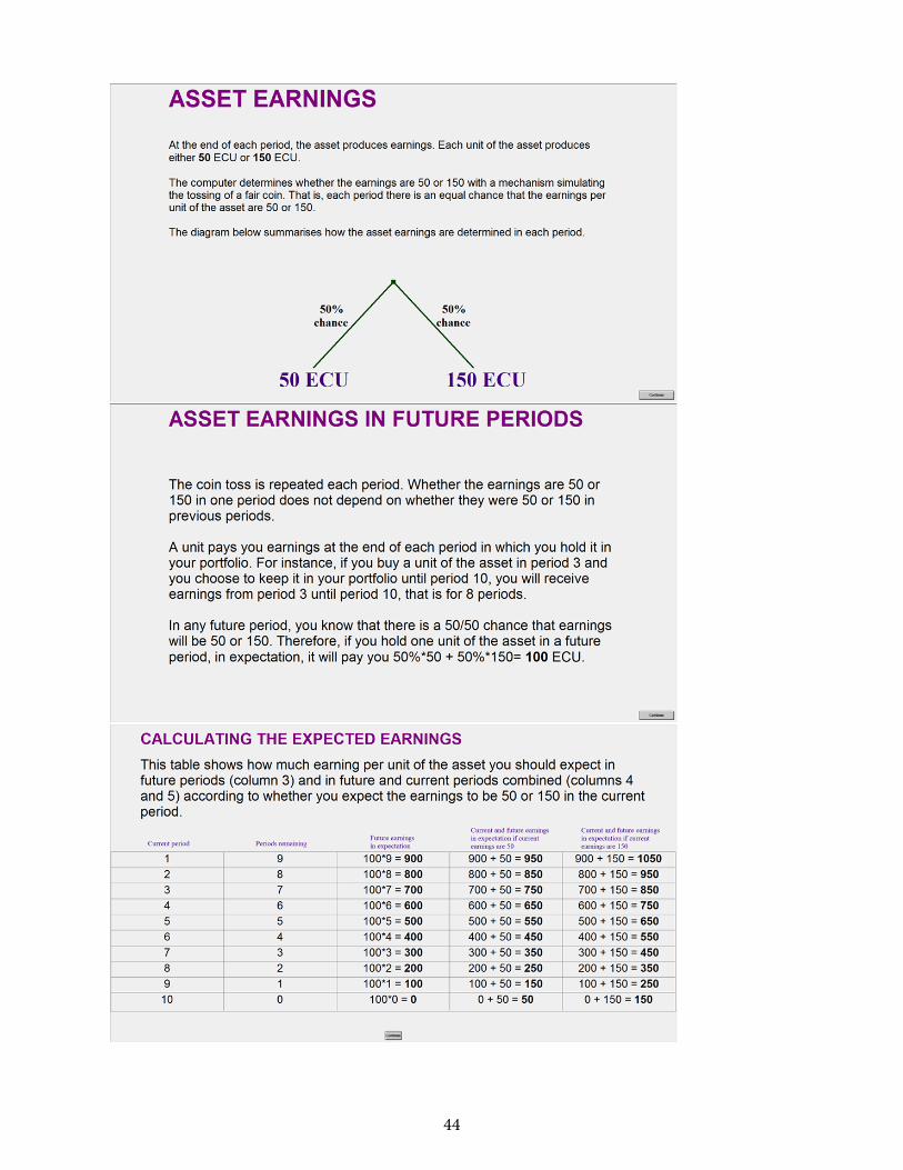
At each period t, the asset yields dividends dt equal to 50 or 150 with equal probability.

Dividends are independently distributed over time. The asset has no residual value after period

10.

The realization of the dividends is unknown to traders. In each period t, however, they receive

noisy private information about the value of the current dividend dt in the form of a symmetric

binary signal with precision 0.75. In particular, each trader i receives a signal sit distributed as

Pr(sit = 0|dt = 50) = Pr(sit = 1|dt = 150) = 0.75. Conditional on the dividend value, signals

are independently distributed. Note that the signal is only informative about the dividend in the

current period, not about future dividends.

At the beginning of the period, half of the traders are selected to pay a fee of 50 for each asset

held in their portfolio at the end of the period. Whether a trader has to pay a fee in a given period

is independent of whether they had to pay it in previous periods.

In period t = 1, each trader has an endowment of 3 assets and 7, 000 of cash. After trading in

6Subjects also answered a series of questionnaires administered to infer non-cognitive abilities (Big-5, Locus ofControl, Grit, Self-Monitoring). We do not describe them here since they are not relevant for this analysis.

7

period t and receiving the dividend, the portfolio of cash and assets carries over to period t + 1.

2.1.2 Equilibrium Prediction

In the Rational Expectations Equilibrium (REE) of the model, the price is equal to the asset’s

fundamental value (i.e., the expected value of current and future dividends). At each period t,

private signals are perfectly aggregated by the price. Moreover, in each period, all traders who

have to pay a fee for holding the asset at the end of the period sell it to those who do not pay the

fee, thereby realizing all the gains from trades.

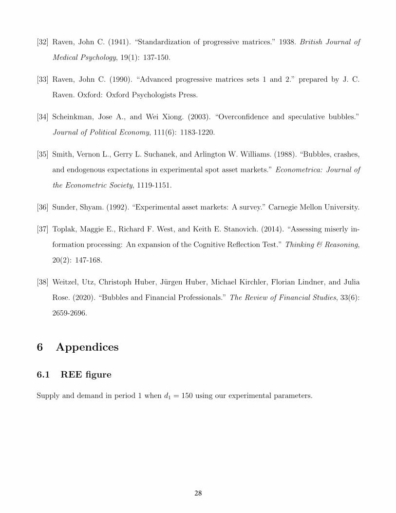
In particular, in period 1, demand and supply clear the market for a price of 950 when d1 = 50

and for a price of 1050 when d1 = 150 (see Figure 6.1 in Appendix): the equilibrium price is equal

to the sum of the expected value of dividends in all subsequent nine periods (100 ∗ 9 = 900) and

the realized dividend in period 1 (50 or 150). The same logic applies to any subsequent period.

Equilibrium prices are reported in Table 1. Note that the equilibrium price of the asset is weakly

decreasing over time: between time t and time t+1, it decreases by 100 (when the dividend is

either 150 or 50 in both periods t and t+1), or by 200 (when the dividend is 150 in period t and

50 in period t+1), or it remains constant (when the dividend is 50 in period t and 150 in period

t+1).

Period (t) t = 1 t = 2 t = 3 t = 4 t = 5 t = 6 t = 7 t = 8 t = 9 t = 10

dt = 50 950 850 750 650 550 450 350 250 150 50dt = 150 1050 950 850 750 650 550 450 350 250 150

Table 1: REE by period and dividend realization

2.1.3 Trading in the laboratory

In the experiment, we have 8 subjects acting as traders. At the beginning of period 1, each subject

receives an endowment of 3 assets and 7, 000 Experimental Currency Units (ECU).

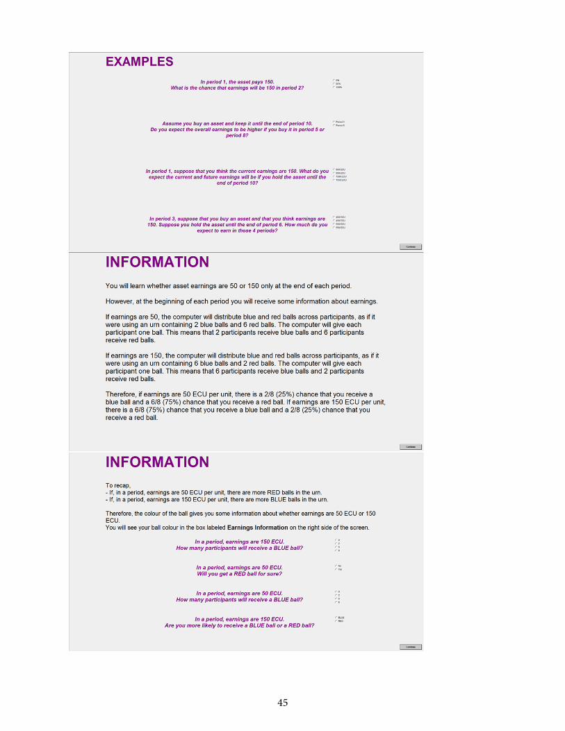
Subjects receive a private signal at the beginning of each period. Specifically, when the dividend

is equal to 150, 6 subjects observe a “blue ball” and 2 subjects a “red ball;” when the dividend

is equal to 50, 6 subjects observe a “red ball” and 2 subjects a “blue ball.” This signal structure

6

guarantees that, in each period, private signals jointly reveal the dividend even if the number of

subjects is finite.7 At the beginning of each period, subjects also learn whether they are fee-paying

or non-fee-paying subjects for that period.

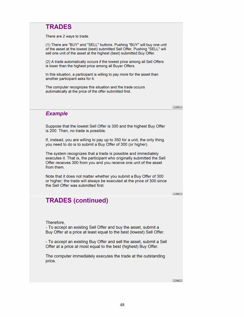
In each period, subjects trade for 150 seconds in a double-auction market. They post offers to

sell or buy one asset. To post a sell offer, a subject enters the minimum price they are willing to

accept and clicks on a sell button. The offer appears immediately on everyone’s screen, in a column

labeled “Sell Offers” (the identity of the subject making the offer is not revealed). Similarly, to

post a buy offer, a subject enters the maximum price they are willing to pay and clicks on a buy

button. A trade is automatically executed whenever the lowest sell offer (ask) is lower than the

highest buy offer (bid).8 Subjects can also buy or sell by clicking on a “BUY” or on a “SELL”

button, which automatically accept the best outstanding sell or buy offer.

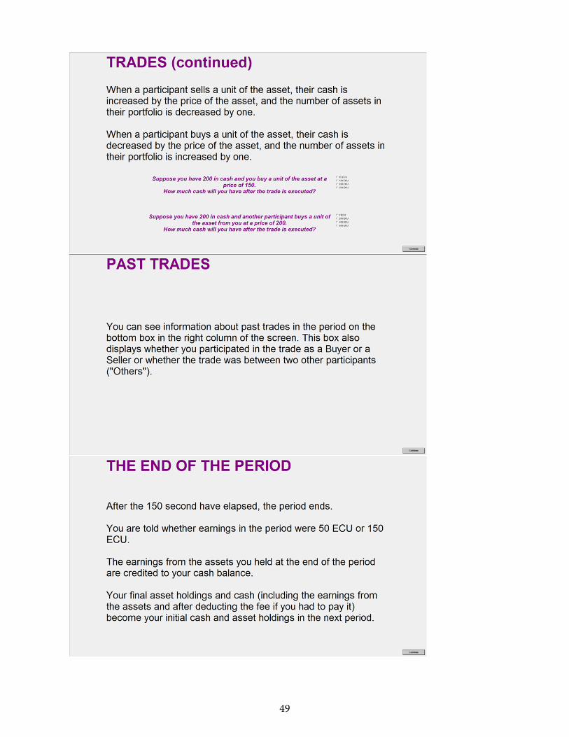
Each subject can post a maximum number of sell offers equal to the number of assets held in

his portfolio; moreover, the sum of all the outstanding buy offers cannot exceed the cash held in his

portfolio. At any time, a subject can withdraw outstanding buy or sell offers that have not already

been executed by clicking a button labeled “Cancel.” A subject’s screen displays their current

portfolio of cash and assets, the list of past trades (with their own executed trades highlighted),

all the outstanding bid and ask prices, and the time left before the end of the period (see sections

6.13 and 6.14 for instructions and decision screen shots).

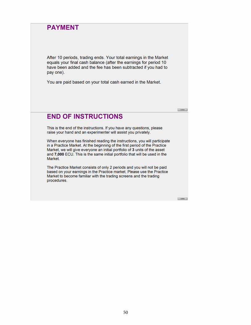
At the end of each period, subjects are informed about the dividend’s realization and their end-

of-period portfolio. Changes in the portfolio between 2 periods are due to the dividends earned,

the fee payments, and the profits or losses from trading. The portfolio at the end of a period carries

over to the next period. After one period ends, trading in the following period starts, according

to the same rules, until all ten periods are completed.

7Other signal structures (for instance, i.i.d. signals with precision 0.75), even if informative, may not deliverthe same result.

8In other words, if a subject wanted, for instance, to buy at the prevailing (i.e., the lowest) ask, they couldsimply enter a price equal to or greater than that price, and the trade would be immediately executed (at theoutstanding price).

7

2.2 The Guessing Game

After the Trading Game, subjects play the standard Guessing Game (GG - Nagel, 1995). Each

subject chooses one number in [0,100]. Subjects are asked to guess a number as close as possible

to a “target” number, defined as 2/3 of the average of the 8 numbers entered by all the subjects

(2/3 is a standard target, used in Nagel’s original paper too). The subject whose number is closest

to the target number earns £5; the others earn nothing. In the case of a tie, the amount is equally

split. The decision screen shot is in Section 6.6.

The only Nash equilibrium of the game is all subjects choosing 0. The most common inter-

pretative framework for behavior in the guessing game is level-k theory. A subject who chooses

randomly in [0,100] is said to be a level-0 subject. A subject who believes that all other subjects are

level-0 and best responds on the basis of this belief, is said to be a level-1 subject. Since a level-1

subject believes that other subjects choose, on average, 50, their best response is to choose 31.8.9

If a subject believes that all others subjects are level-1 and best responds accordingly, they choose

21.2 and are said to be a level-2 subject. In general, a level-k subject is one who best responds to

the belief that others are level-(k-1) subjects. When k tends to infinity, the best response converges

to the Nash equilibrium action.

2.3 The Individual Guessing Game

After this standard GG, we ask subjects to take part in a modified, individual-level version of

the GG. In this Individual Guessing Game (IGG), each subject chooses 8 numbers and the target

number is 2/3 times the average of these 8 numbers. One of the subject’s 8 chosen numbers is

randomly selected for payment and, if it equals the target number, the subject earns £5. The

decision screen shot is in Section 6.7.

As we explained above, according to level-k theory, subjects with higher levels of strategic

reasoning choose lower numbers in the GG. However, for any choice in the GG between 1 and 50,

one cannot disentangle a subject’s level of reasoning from the subject’s belief about other subjects’

levels of reasoning. For instance, suppose a subject chooses 31.8 and is, therefore, classified as a

9This number slightly differs from 33.3 since the average takes the subject’s own guess into account.

8

level-1 subject. This choice could be because the subject lacks the ability to reason past level 1;

or it could be because, although the subject does have such an ability, they believe that other

subjects are level-0 subjects.

Our novel IGG disentangles one own’s ability and their belief about the ability of others. In

particular, in the IGG, the only 8 numbers that guarantees earning £5 are all zeros. A subject

who enters this answer has the ability to reason to an arbitrarily high level. Therefore, using the

example above, if a subject chooses 31.8 in the GG and correctly answers the IGG, they show a

high level of strategic thinking ability but a low-level belief about the strategic sophistication of

their peers.

2.4 Individual-level tasks

We use individual-level tasks to collect data on cognitive abilities, risk preferences, and confi-

dence.10

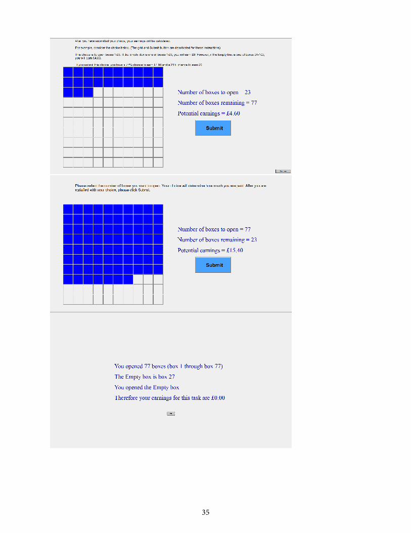
2.4.1 Risk Preferences - Bomb Risk Elicitation Task (BRET)

To measure risk preferences, we employ the “Bomb Risk Elicitation Task” (BRET, Crosetto and

Filippin, 2013). In the BRET, subjects are shown a screen with 100 boxes and are asked to choose

to “open a number of boxes” (between 1 and 99). Each box contains 20 pence; therefore, earnings

increase linearly with the number of boxes chosen. Among the boxes, however, there is one that, if

chosen, makes the subject lose all their earnings (in the original version by Crosetto and Filippin

(2013) this box was described as a box containing a bomb; we used a more neutral description).11

Since all boxes appear the same, the decision about the number of boxes is a decision under

risk. A risk-neutral subject collects 50 boxes. A risk-averse subject collects less than 50 boxes

and a risk-loving one more than 50. The more boxes a subjects collects the higher their degree of

risk-seeking preference. BRET is the only task described in Section 2.4 that is incentivized.

10We also collect data on other non-cognitive traits not discussed in this paper.11For a comparison of different risk elicitation methods, see Crosetto and Filippin (2016).

9

2.4.2 Cognitive Ability - Raven’s matrices (IQ)

Our first test of cognitive ability is the Raven’s (1941) progressive matrices test (perhaps, the most

well-known IQ test). We selected 18 of the most difficult Raven’s matrices, available in Raven’s

Advanced Progressive Matrices (Raven, 1990). We did this to avoid a ceiling effect on the scores

(which we did, as the highest score recorded was 15 out of 18). A subject’s IQ score is the number

of correct answers within a 10-minute period.

2.4.3 Cognitive Ability - Cognitive Reflection Test (CRT)

Our second test of cognitive ability is the Cognitive Reflection Test (Frederick, 2005). The test is

designed to measure a subject’s tendency to override an incorrect impulsive response and engage

in further reflection that leads to the correct answer. For instance, one question is the following:

“A bat and a ball cost £1.10 in total. The bat costs one pound more than the ball. How much

does the ball cost?” An answer of 5 pence is correct while an answer of 10 pence suggests a lack

of reflection.

We use the extended 7-question version of the CRT (Toplak, West, and Stanovich, 2014). A

subject’s CRT score is the number of correct answers within a 5-minute period.

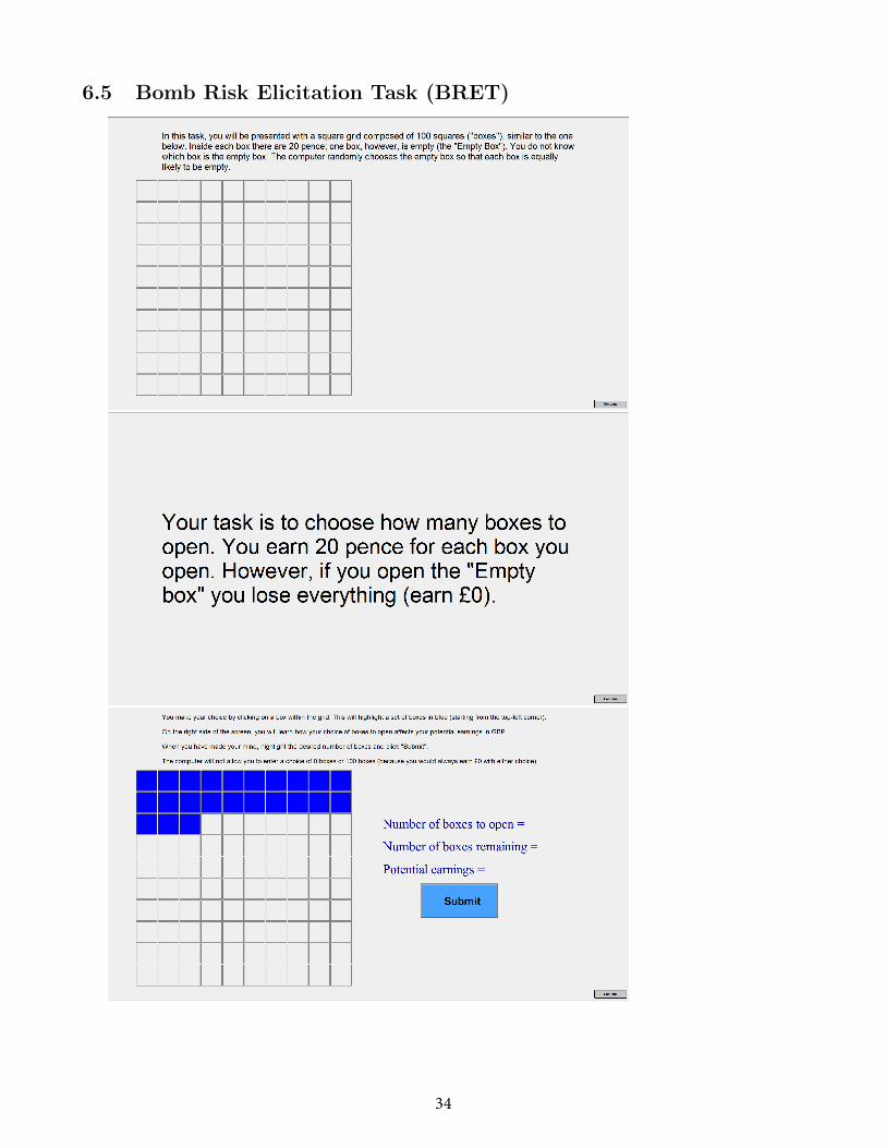
2.4.4 Confidence

After the Raven test and after the CRT, we present subjects with an 8-row table, in which each row

reads: “What is the percent chance that X of the 7 other participants had more correct answers

than you did?” (for X = {0,1,...7}). In other words, we elicit the entire distribution of beliefs about

the subject’s ranking for each of these two cognitive ability tests. Given the subject’s answers, for

each test, we compute the expected number of outperforming subjects. The difference between

the actual and expected numbers is our confidence measure for the subject. A positive number

indicates that the subject is over-confident (because they expected to be outperformed by fewer

subjects than was the case); a negative number indicates that the subject is under-confident; and a

score of 0 means that the subject is not biased. As we said, for each subject, we have this measure

for both the Raven and the CRT test. We average these measures to get the composite measure

10

of confidence, which we use in Section 4.3.

3 Experimental Subjects

We ran the experiment in the Experimental Laboratory for Finance and Economics (ELFE) in the

Centre for Finance at the Department of Economics at UCL.

We ran two treatments, the “Trader Treatment” and the “Student Treatment.” The two treat-

ments differ in the pool of subjects. In the Trader Treatment, the subjects are traders and portfolio

managers working in London (UK). In the Student Treatment, subjects are UCL undergraduate

students from all disciplines; we use the Student Treatment as our control treatment.

Each treatment consists of 7 sessions; in each session, 8 subjects perform the tasks described

above. Overall, our sample includes 56 professional traders and 56 undergraduate students. Sub-

jects had no previous experience with this experiment and participate in one session only. Each

session lasted approximately 2 hours.

The subject pool for the Trader Treatment consists of: 30 traders, 4 proprietary traders, 4

sales-traders, 12 portfolio managers, and 6 belonging to other categories (e.g., trading strategists

or sales with management of virtual portfolios).12 Subjects work in a variety of financial markets,

such as equity, equity derivatives, FX, fixed income, and commodities. Thirty-two subjects are

employed by an investment bank, 12 by an investment fund and the others by other types of

institutions (or chose not to report). Traders’ age ranges between 22 and 48 years, with a mean

of 32 years and a standard deviation of 6.17 years. Their average job tenure is 9.25 years, with a

range between 1.5 and 21 years (standard deviation: 5.42 years). Three subjects have an MPhil or

Ph.D., 30 a Master degree, 4 an MBA, 19 a Bachelor degree. Thirty subjects studied economics

or finance, 8 mathematics or physics, 8 engineering or computer science, and the remaining have

a degree in other disciplines or did not declare it.

In our Student treatment, we use UCL undergraduate students from all disciplines. We chose

12In our call for subjects, we wrote that “we need participants who are either traders or portfolio managers orwho have had such roles in the past. You are also eligible if you do not have the formal title of trader or portfoliomanagers, but you perform activities that are closely related to that of a trader or portfolio manager (e.g., sales-trader or sales on the trading floor)”. The call for subjects is in Section 6.12.

11

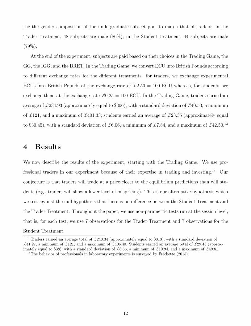
the the gender composition of the undergraduate subject pool to match that of traders: in the

Trader treatment, 48 subjects are male (86%); in the Student treatment, 44 subjects are male

(79%).

At the end of the experiment, subjects are paid based on their choices in the Trading Game, the

GG, the IGG, and the BRET. In the Trading Game, we convert ECU into British Pounds according

to different exchange rates for the different treatments: for traders, we exchange experimental

ECUs into British Pounds at the exchange rate of £2.50 = 100 ECU whereas, for students, we

exchange them at the exchange rate £0.25 = 100 ECU. In the Trading Game, traders earned an

average of £234.93 (approximately equal to $306), with a standard deviation of £40.53, a minimum

of £121, and a maximum of £401.33; students earned an average of £23.35 (approximately equal

to $30.45), with a standard deviation of £6.06, a minimum of £7.84, and a maximum of £42.50.13

4 Results

We now describe the results of the experiment, starting with the Trading Game. We use pro-

fessional traders in our experiment because of their expertise in trading and investing.14 Our

conjecture is that traders will trade at a price closer to the equilibrium predictions than will stu-

dents (e.g., traders will show a lower level of mispricing). This is our alternative hypothesis which

we test against the null hypothesis that there is no difference between the Student Treatment and

the Trader Treatment. Throughout the paper, we use non-parametric tests run at the session level;

that is, for each test, we use 7 observations for the Trader Treatment and 7 observations for the

Student Treatment.

13Traders earned an average total of £240.34 (approximately equal to $313), with a standard deviation of£41.27, a minimum of £121, and a maximum of £406.40. Students earned an average total of £29.43 (approx-imately equal to $38), with a standard deviation of £8.65, a minimum of £10.94, and a maximum of £49.81.

14The behavior of professionals in laboratory experiments is surveyed by Frechette (2015).

12

4.1 The Trading Game

4.1.1 Bubbles

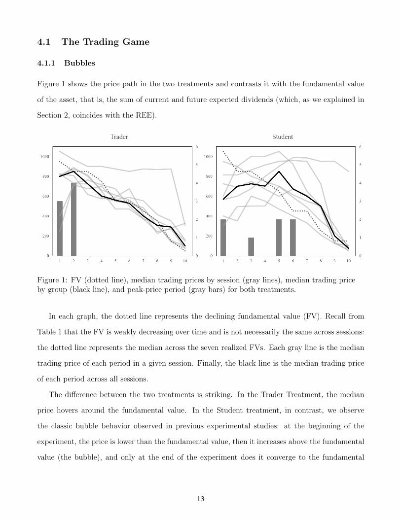
Figure 1 shows the price path in the two treatments and contrasts it with the fundamental value

of the asset, that is, the sum of current and future expected dividends (which, as we explained in

Section 2, coincides with the REE).

Figure 1: FV (dotted line), median trading prices by session (gray lines), median trading priceby group (black line), and peak-price period (gray bars) for both treatments.

In each graph, the dotted line represents the declining fundamental value (FV). Recall from

Table 1 that the FV is weakly decreasing over time and is not necessarily the same across sessions:

the dotted line represents the median across the seven realized FVs. Each gray line is the median

trading price of each period in a given session. Finally, the black line is the median trading price

of each period across all sessions.

The difference between the two treatments is striking. In the Trader Treatment, the median

price hovers around the fundamental value. In the Student treatment, in contrast, we observe

the classic bubble behavior observed in previous experimental studies: at the beginning of the

experiment, the price is lower than the fundamental value, then it increases above the fundamental

value (the bubble), and only at the end of the experiment does it converge to the fundamental

13

value.15

To quantify the mispricing, we use the Relative Absolute Deviation (RAD) measure commonly

used in the experimental bubble literature. In each period of each session, we compute the absolute

difference between that period’s observed average price and the FV. The average of these absolute

differences across all ten periods of a session divided by the average FV of the session is the session’s

RAD measure. Intuitively, the RAD captures the percentage difference, across all periods, between

the average mean prices per period and the average FV. The 14 RAD measures (one for each session

of each treatment) are in Table 2. The average RAD in the Trader Treatment is 22.5%, whereas the

average RAD in the Student Treatment is almost twice as large, 39.2%. Testing the null hypothesis

of no difference across groups against the alternative hypothesis that the Trader Treatment will has

lower levels of mispricing, we reject the null at the p-value= 0.049 level (one-sided Mann-Whitney

U -test).

1 2 3 4 5 6 7 Avg.Trader sessions .241 .280 .206 .534 .060 .134 .124 .225Student sessions .457 .411 .343 .756 .393 .239 .146 .392

p-value 0.049

Table 2: RAD by session

Table 3 displays the average RAD across sessions, computed for each period and each treat-

ment.16

Period (t) t = 1 t = 2 t = 3 t = 4 t = 5 t = 6 t = 7 t = 8 t = 9 t = 10

Traders 28% 14% 14% 12% 15% 21% 24% 30% 70% 112%Students 38% 28% 17% 20% 27% 60% 62% 112% 100% 107%p-value 0.104 0.036 0.451 0.191 0.130 0.013 0.019 0.006 0.690 0.841

Table 3: Relative absolute deviations (average) by period and group. We report p-values for one-sided Mann-Whitney U tests for differences between traders and students.

In periods 6, 7, and 8, traders had significantly lower RADs than students, with one-sided

Mann-Whitney U tests p-values of 0.013, 0.019 and 0.006. These are the periods when the students

create a bubble whereas the traders trade at price close to the FV.

15The figures look similar using means rather than medians (see Section 6.2).16The RAD is a measure of percentage deviation. As shown in the table, the RAD increases over the periods,

due to the fact that subjects’ pricing errors remains roughly constant.

14

In Figure 1, for each period, we also report (in dark-gray bars) the number of sessions (on

the vertical axis on the right) in which the median trading price reached the highest level in that

period. For the Trader treatment, all seven sessions had their peak price in the first two periods,

consistent with the fact that fundamental value is weakly declining;17 in contrast, in the Student

Treatment, in four sessions out of seven the peak is reached in periods 5 or 6, consistent with

the fact in this treatment we observe bubbles. This measure is different across treatments with a

p-value= 0.049 level (one-sided Mann-Whitney U -test).18

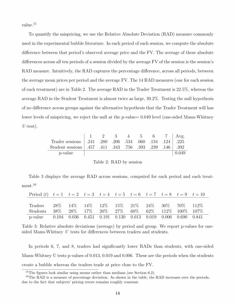
Figure 2 displays the median deviation between price and FV across periods and treatments.

Specifically, for every trade, we compute the difference between its price and the actual FV of

the asset in that period. Figure 2 reports the median of these differences. As the figure shows,

the Student Treatment follows the classic bubble pattern (the price is below the FV in the early

periods, above the FV in the middle periods, and ends close to the FV at the end of the experiment),

whereas the Trader Treatment does not.

Figure 2: Difference between median price and FV by period

As a final observation, note that in the Student Treatment there is substantial heterogeneity

across sessions. In contrast, in the Trader Treatment, behavior in six sessions is very homogeneous;

17In our study, if d1 = 50 and d2 = 150, then the theory predicts that the price in periods 1 and 2 should bothbe 950. An experimental market with these dividend realizations would align with the theory if it had a peakprice at either period 1 or 2. For any other dividend realization, the theoretically predicted peak price is uniqueat period 1.

18The periods with the highest median price for the 7 sessions in the Trader Treatment are {1, 1, 1, 2, 2, 2, 2}.For the Student Treatment, the periods are {1, 1, 3, 5, 5, 6, 6}. The null of the test is that the set of periods hasthe same central tendency. is the same.

15

one session is an outlier, with traders unable to track the fundamental value. Importantly, not

even this session shows the standard bubble pattern we observe in the Student Treatment and

in previous experiments. Indeed, in the first round subjects trade at prices higher than the FV

(whereas in typical bubble experiments the price is lower than the FV); moreover, the price remains

higher than the FV even in the last round (whereas in typical bubble experiments the price crashes

and becomes close to the FV).

Finally, in the REE, all assets are held by subjects who are not required to pay a fee thus

realizing all gains from trade. In the experiment, since the fee is paid at the end of the period,

subjects have the opportunity to gain from trade. If, instead, they do not trade or trade without

accounting for the fee, then, on average, 50% of assets are held by non-fee-paying subjects. In the

Student Treatment, only 56% of assets are held (at the end of the period) by non-fee-paying sub-

jects. If we restrict the analysis to the last 3 periods, allocative efficiency is only marginally better,

with 62% of assets held by non-fee-paying subjects. In the Trader Treatment, the frequencies are

57% for all periods and 62% for the last 3 periods. Essentially, even in the Trader Treatment,

allocative efficiency seems to have been sacrificed to other aspects of the market environment. At

least within the period of time they were allowed to trade, both students and traders did not

manage to realize all the gains from trade.

4.1.2 Information Aggregation

As we explained in Section 2, at the beginning of each period, subjects receive information about

the current period’s dividend. The question we want to answer is whether (or to what extent) this

information is used in the experiment.

Recall that in the REE, private information is fully aggregated. The change of price between t

and t+1 depends on two components: the fact that between time t and time t-1 time-t dividend is

paid out (and therefore should not be reflected in time t+1 price); and the fact that the t+1 price

reflects the t+1-dividend’s realization. In particular, as shown in Table 1, moving from period t

to period t + 1, three situations can occur: dt = 150 and dt+1 = 50, in which case the REE price

drops by 200; dt = 150 and dt+1 = 150 or dt = 50 and dt+1 = 50, in which case the REE price

16

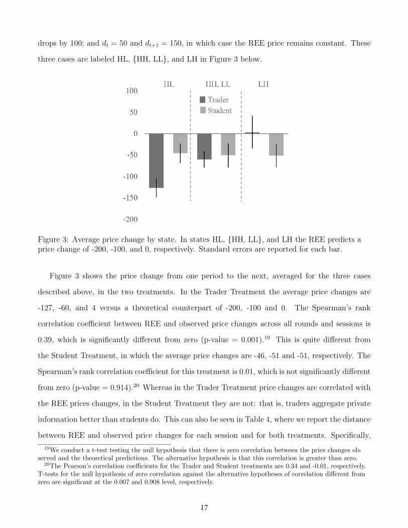
drops by 100; and dt = 50 and dt+1 = 150, in which case the REE price remains constant. These

three cases are labeled HL, {HH, LL}, and LH in Figure 3 below.

Figure 3: Average price change by state. In states HL, {HH, LL}, and LH the REE predicts aprice change of -200, -100, and 0, respectively. Standard errors are reported for each bar.

Figure 3 shows the price change from one period to the next, averaged for the three cases

described above, in the two treatments. In the Trader Treatment the average price changes are

-127, -60, and 4 versus a theoretical counterpart of -200, -100 and 0. The Spearman’s rank

correlation coefficient between REE and observed price changes across all rounds and sessions is

0.39, which is significantly different from zero (p-value = 0.001).19 This is quite different from

the Student Treatment, in which the average price changes are -46, -51 and -51, respectively. The

Spearman’s rank correlation coefficient for this treatment is 0.01, which is not significantly different

from zero (p-value = 0.914).20 Whereas in the Trader Treatment price changes are correlated with

the REE prices changes, in the Student Treatment they are not: that is, traders aggregate private

information better than students do. This can also be seen in Table 4, where we report the distance

between REE and observed price changes for each session and for both treatments. Specifically,

19We conduct a t-test testing the null hypothesis that there is zero correlation between the price changes ob-served and the theoretical predictions. The alternative hypothesis is that this correlation is greater than zero.

20The Pearson’s correlation coefficients for the Trader and Student treatments are 0.34 and -0.01, respectively.T-tests for the null hypothesis of zero correlation against the alternative hypotheses of correlation different fromzero are significant at the 0.007 and 0.908 level, respectively.

17

in each period from 2 to 10, we compute the absolute difference between the average price change

and the REE one. We then average this error across all 9 periods in that session. This provides a

session-level measure for how well the actual price change matched the theoretically predicted price

change. In the Trader Treatment, the average distance is 81.1, whereas in the Student Treatment

it is 121.8. The difference is statistically significant (one-sided Mann-Whitney U test p-value =

0.011).

Session 1 2 3 4 5 6 7 Avg.Trader Treatment 92.4 91.9 81.1 109.0 41.0 89.3 63.3 81.1Student Treatment 158.4 135.0 112.8 151.5 115.0 108.4 71.4 121.8

p-value 0.011

Table 4: Average absolute difference between price change and predicted FV change by session.

Note that (the lack of) information aggregation is a separate issue from (the absence of) bubbles.

In particular, students might have engaged in bubble behavior and still made use of their signals:

in this case, the change in price from one period to the next would still be related to dividends’

realizations. Similarly, traders could have failed to use private information, while still keeping the

price around the fundamental value: this would have entailed, for instance, reducing the price by

100 (the unconditional expected change) each period.

4.2 Guessing Games

We now turn to the analysis of subject’s behavior in the Guessing Games. We start with the

standard GG and then we move to the individual decision making version of it (IGG).

4.2.1 Guessing Game

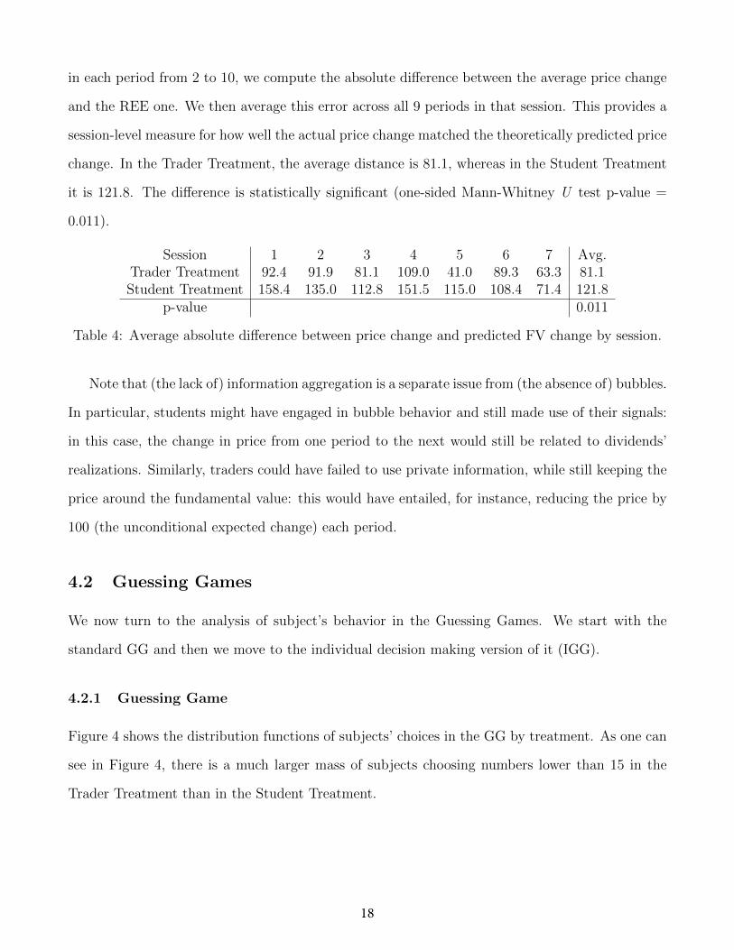
Figure 4 shows the distribution functions of subjects’ choices in the GG by treatment. As one can

see in Figure 4, there is a much larger mass of subjects choosing numbers lower than 15 in the

Trader Treatment than in the Student Treatment.

18

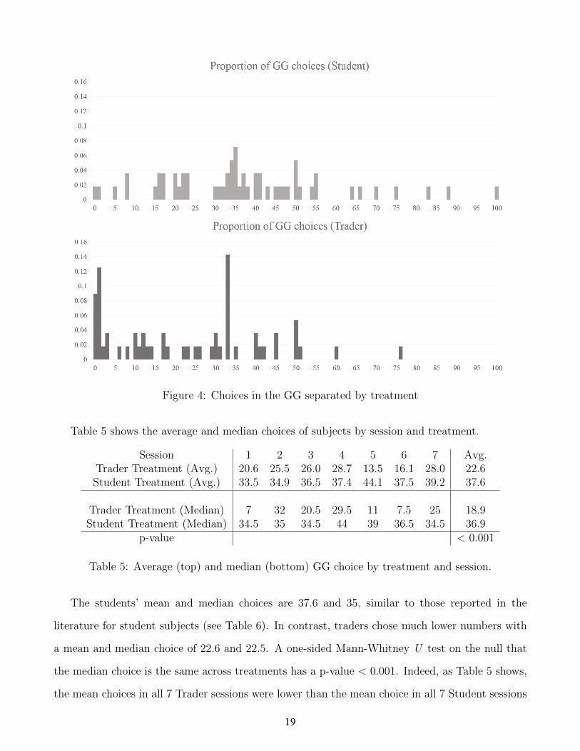
Figure 4: Choices in the GG separated by treatment

Table 5 shows the average and median choices of subjects by session and treatment.

Session 1 2 3 4 5 6 7 Avg.Trader Treatment (Avg.) 20.6 25.5 26.0 28.7 13.5 16.1 28.0 22.6Student Treatment (Avg.) 33.5 34.9 36.5 37.4 44.1 37.5 39.2 37.6

Trader Treatment (Median) 7 32 20.5 29.5 11 7.5 25 18.9Student Treatment (Median) 34.5 35 34.5 44 39 36.5 34.5 36.9

p-value < 0.001

Table 5: Average (top) and median (bottom) GG choice by treatment and session.

The students’ mean and median choices are 37.6 and 35, similar to those reported in the

literature for student subjects (see Table 6). In contrast, traders chose much lower numbers with

a mean and median choice of 22.6 and 22.5. A one-sided Mann-Whitney U test on the null that

the median choice is the same across treatments has a p-value < 0.001. Indeed, as Table 5 shows,

the mean choices in all 7 Trader sessions were lower than the mean choice in all 7 Student sessions

19

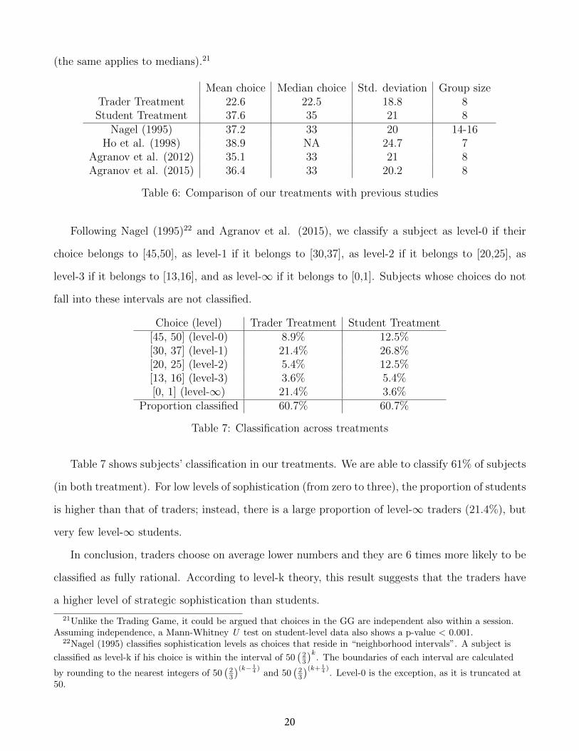
(the same applies to medians).21

Mean choice Median choice Std. deviation Group sizeTrader Treatment 22.6 22.5 18.8 8Student Treatment 37.6 35 21 8

Nagel (1995) 37.2 33 20 14-16Ho et al. (1998) 38.9 NA 24.7 7

Agranov et al. (2012) 35.1 33 21 8Agranov et al. (2015) 36.4 33 20.2 8

Table 6: Comparison of our treatments with previous studies

Following Nagel (1995)22 and Agranov et al. (2015), we classify a subject as level-0 if their

choice belongs to [45,50], as level-1 if it belongs to [30,37], as level-2 if it belongs to [20,25], as

level-3 if it belongs to [13,16], and as level-∞ if it belongs to [0,1]. Subjects whose choices do not

fall into these intervals are not classified.

Choice (level) Trader Treatment Student Treatment[45, 50] (level-0) 8.9% 12.5%[30, 37] (level-1) 21.4% 26.8%[20, 25] (level-2) 5.4% 12.5%[13, 16] (level-3) 3.6% 5.4%[0, 1] (level-∞) 21.4% 3.6%

Proportion classified 60.7% 60.7%

Table 7: Classification across treatments

Table 7 shows subjects’ classification in our treatments. We are able to classify 61% of subjects

(in both treatment). For low levels of sophistication (from zero to three), the proportion of students

is higher than that of traders; instead, there is a large proportion of level-∞ traders (21.4%), but

very few level-∞ students.

In conclusion, traders choose on average lower numbers and they are 6 times more likely to be

classified as fully rational. According to level-k theory, this result suggests that the traders have

a higher level of strategic sophistication than students.

21Unlike the Trading Game, it could be argued that choices in the GG are independent also within a session.Assuming independence, a Mann-Whitney U test on student-level data also shows a p-value < 0.001.

22Nagel (1995) classifies sophistication levels as choices that reside in “neighborhood intervals”. A subject is

classified as level-k if his choice is within the interval of 50(23

)k. The boundaries of each interval are calculated

by rounding to the nearest integers of 50(23

)(k− 14 ) and 50

(23

)(k+ 14 ). Level-0 is the exception, as it is truncated at

50.

20

4.2.2 Individual Guessing Game

According to level-k theory, a subject choosing approximately 30 in the GG is classified as level-1,

a low level of sophistication. It is unclear, however, whether the choice of 30 is due to lack of

ability (i.e., the subject is not sophisticated in their understanding of the game) or to the belief

that all other subjects choose randomly (i.e, they are level-0). With the IGG, we study subjects’

behavior in a task in which beliefs about others are irrelevant. A subject who chooses numbers

different from 0 in the IGG does not understand the game (regardless of their beliefs about others).

More importantly, a subject who chooses all 0s in the IGG but who chooses a higher number in

the original GG must have done so based on their belief about the rationality of others.

In our experiment, the proportion of subjects able to solve the IGG is virtually identical in the

two samples: 11 traders and 10 students correctly answered all zeros (the two proportions are not

statistically different, with a p-value = 0.87).23 It is interesting to see how this subset of subjects

acted in the original GG (Figure 5). The mean and median choice (11.73 and 3, respectively)

of traders is significantly lower than the mean and median choice (26.8 and 31.5, respectively)

of students (one-sided Mann-Whitney U test p-value = 0.019). By correctly answering the IGG,

the 11 traders and 10 students showed that they had the intellectual ability to solve the game.

The difference in their GG choices must come from different beliefs about their competitors’

choices. The Trader subgroup guessed significantly lower numbers than the Student subgroup.

This indicates that traders believed (correctly) that their opponents had a higher strategic level

of reasoning compared to the beliefs of students.

23Five students and six traders did not enter their numbers in time.

21

Figure 5: Choices in the GG of the subjects who correctly answered the IGG.

The different choices in the original GG between traders and students is not only driven by

differences in these subgroups (i.e., students and traders who solve the IGG). When analyzing

the choices in the GG of subjects who did not correctly solve the IGG, we still observe that the

mean choice of traders (25.3) is significantly lower than the mean choice of students (39.9), with

a one-sided Mann-Whitney U test p-value < 0.001.

Interestingly, 5 of the 10 subjects in this student subgroup were classified as level-1 in the GG.

Put differently, 33% of the student subjects who are classified as level-1 in the GG actually show

an arbitrarily high level of rationality (because they correctly solved the IGG). This suggests that

the IGG could be used to further refine levels in future research using guessing games. In addition,

one may wonder whether the 21 subjects who correctly solved the IGG were also closer to the

target in the GG. The answer is no. The 46 students who did not correctly solve the IGG were, on

average, 15.8 away from the target while the 10 students who correctly solved it were 15.1 away.

For the traders, the 45 who did not correctly solve the IGG were, on average, 15.5 away from

the target while the other 11 traders who correctly solved it were 13.4 away. In both cases, the

distances from the target are not statistically different (one-sided Mann-Whitney U test p-value

= 0.460 for students and 0.359 for traders).

22

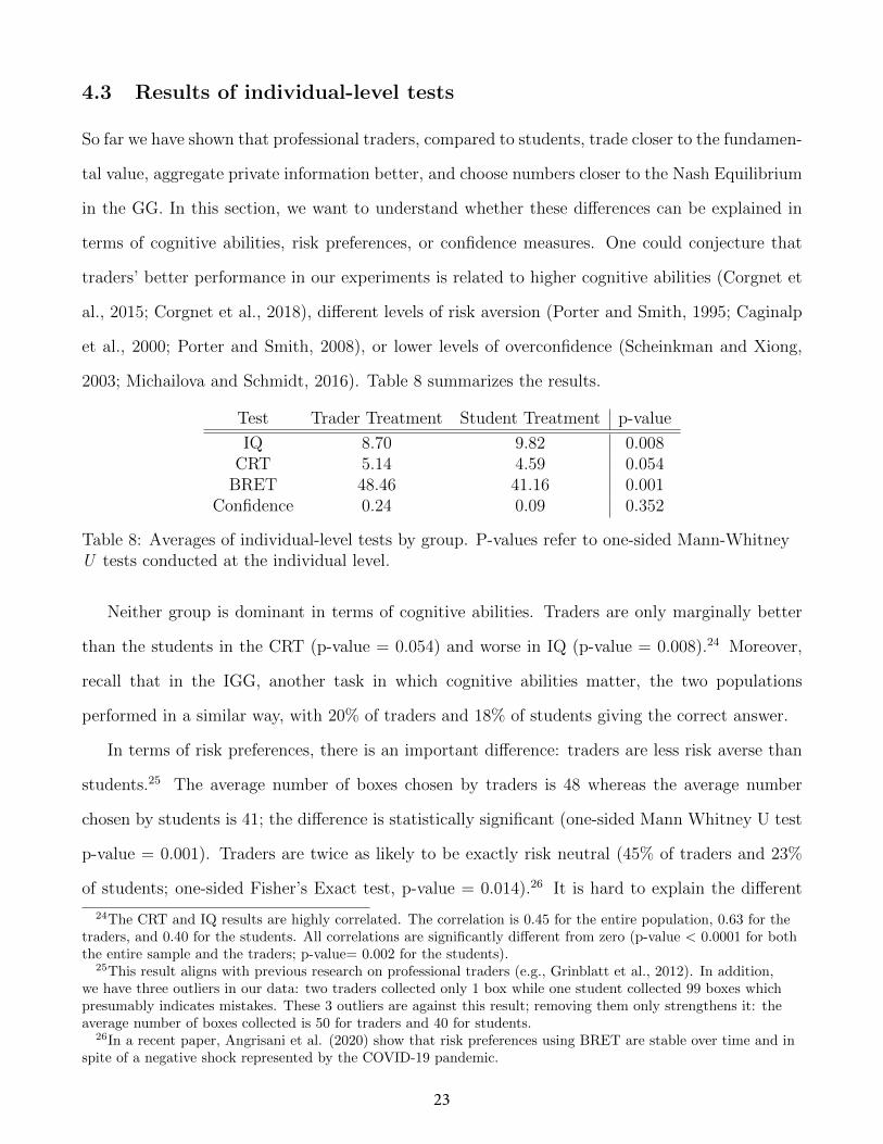
4.3 Results of individual-level tests

So far we have shown that professional traders, compared to students, trade closer to the fundamen-

tal value, aggregate private information better, and choose numbers closer to the Nash Equilibrium

in the GG. In this section, we want to understand whether these differences can be explained in

terms of cognitive abilities, risk preferences, or confidence measures. One could conjecture that

traders’ better performance in our experiments is related to higher cognitive abilities (Corgnet et

al., 2015; Corgnet et al., 2018), different levels of risk aversion (Porter and Smith, 1995; Caginalp

et al., 2000; Porter and Smith, 2008), or lower levels of overconfidence (Scheinkman and Xiong,

2003; Michailova and Schmidt, 2016). Table 8 summarizes the results.

Test Trader Treatment Student Treatment p-value

IQ 8.70 9.82 0.008CRT 5.14 4.59 0.054

BRET 48.46 41.16 0.001Confidence 0.24 0.09 0.352

Table 8: Averages of individual-level tests by group. P-values refer to one-sided Mann-WhitneyU tests conducted at the individual level.

Neither group is dominant in terms of cognitive abilities. Traders are only marginally better

than the students in the CRT (p-value = 0.054) and worse in IQ (p-value = 0.008).24 Moreover,

recall that in the IGG, another task in which cognitive abilities matter, the two populations

performed in a similar way, with 20% of traders and 18% of students giving the correct answer.

In terms of risk preferences, there is an important difference: traders are less risk averse than

students.25 The average number of boxes chosen by traders is 48 whereas the average number

chosen by students is 41; the difference is statistically significant (one-sided Mann Whitney U test

p-value = 0.001). Traders are twice as likely to be exactly risk neutral (45% of traders and 23%

of students; one-sided Fisher’s Exact test, p-value = 0.014).26 It is hard to explain the different

24The CRT and IQ results are highly correlated. The correlation is 0.45 for the entire population, 0.63 for thetraders, and 0.40 for the students. All correlations are significantly different from zero (p-value < 0.0001 for boththe entire sample and the traders; p-value= 0.002 for the students).

25This result aligns with previous research on professional traders (e.g., Grinblatt et al., 2012). In addition,we have three outliers in our data: two traders collected only 1 box while one student collected 99 boxes whichpresumably indicates mistakes. These 3 outliers are against this result; removing them only strengthens it: theaverage number of boxes collected is 50 for traders and 40 for students.

26In a recent paper, Angrisani et al. (2020) show that risk preferences using BRET are stable over time and inspite of a negative shock represented by the COVID-19 pandemic.

23

behavior in the Trading Game or in the GG in terms of different levels of risk aversion. Risk

averse agents value the asset less than in the risk-neutral theoretical benchmark. As a result, in

the Trading Game, lower traders’ risk aversion should generate more, not less overpricing than in

the students’ treatment. Moreover, risk preferences do not play a role in the GG, since each agent

simply maximizes the probability of winning the prize.

Finally, one may conjecture that overconfidence could lead to bubbles, with subjects believing

that they can outplay the others and sell off their assets before the bubble bursts. However, our

confidence measures for the Trader Treatment and the Student Treatment are not statistically

different from each other (p-value=0.352); if anything, in our sample, traders’ overconfidence is

higher than students’. In addition, it is important to remark that our confidence measures are

not statistically different from 0 in either treatment (with a p-value equal to 0.340 in the Trader

Treatment and 0.679 in the Student Treatment).

In summary, the differences we observe in terms of asset pricing, information aggregation,

and Guessing Game choices are not related to cognitive abilities, risk preferences, or confidence.

Differences between traders and students may be due to skills that professional traders learn on

the job or to their beliefs about the strategies of other traders (indeed, the evidence from the GG

and the IGG shows that traders believe that their peers use higher strategic thinking than do

students).

5 Conclusion

We have studied how professional traders behave in laboratory experiments (a trading game and a

guessing game) which are informative of financial market behavior. We have found that, compared

to undergraduate students, choices made by professional traders more closely align with equilibrium

predictions. In a trading experiment with traders subjects, prices are closer to the fundamental

value and bubbles do not occur. Moreover, private information is aggregated to a greater extent. In

the guessing game, traders exhibit a higher ability to reason strategically. The differences between

traders and students are not due to differences in cognitive abilities, risk aversion, or confidence.

24

References

[1] Agranov, Marina, Elizabeth Potamites, Andrew Schotter, and Chloe Tergiman. (2012). “Be-

liefs and endogenous cognitive levels: An experimental study.” Games and Economic Behav-

ior, 75(2): 449-463.

[2] Agranov, Marina, Andrew Caplin, and Chloe Tergiman. (2015). “Naive play and the process

of choice in guessing games.” Journal of the Economic Science Association, 1(2): 146-157.

[3] Alevy, Jonathan E., Michael S. Haigh, and John A. List. (2007). “Information cascades:

Evidence from a field experiment with financial market professionals.” The Journal of Finance,

62(1): 151-180.

[4] Angrisani, Marco, Marco Cipriani, Antonio Guarino, Ryan Kendall, and Julen Ortiz de Zarate

Pina. (2020). “Risk Preferences at the Time of COVID-19: An Experiment with Professional

Traders and Students.” Staff Reports 927, Federal Reserve Bank of New York.

[5] Caginalp, Gunduz, David Porter, and Vernon L. Smith. (2000). “Overreaction, momentum,

liquidity, and price bubbles in laboratory and field asset markets.” Journal of Psychology and

Financial Markets, 1: 24-48.

[6] Cason, Timothy N., and Daniel Friedman. (1997). “Price formation in single call markets.”

Econometrica: Journal of the Econometric Society, 311-345.

[7] Cipriani, Marco, and Antonio Guarino. (2005). “Herd behavior in a laboratory financial mar-

ket.” American Economic Review, 95.5: 1427-1443.

[8] Cipriani, Marco, and Antonio Guarino. (2009). “Herd behavior in financial markets: an exper-

iment with financial market professionals.” Journal of the European Economic Association,

7(1): 206-233.

[9] Corgnet, Brice, Mark DeSantis, and David Porter. (2015). “Revisiting information aggregation

in asset markets: Reflective learning & market efficiency.” Working paper.

25

[10] Corgnet, Brice, Mark DeSantis, and David Porter. (2018). “What makes a good trader? On

the role of intuition and reflection on trader performance.” The Journal of Finance, 73(3):

1113-1137.

[11] Crosetto, Paolo, and Antonio Filippin. (2013). “The “bomb” risk elicitation task.” Journal of

Risk and Uncertainty, 47(1): 31-65.

[12] Crosetto, Paolo, and Antonio Filippin. (2016). “A theoretical and experimental appraisal of

four risk elicitation methods.” Experimental Economics, 19(3): 613-641.

[13] Frechette, Guillaume R. (2015). “Laboratory Experiments: Professionals versus Students.” In

Handbook of Experimental Economic Methodology, Oxford University Press. 360-390.

[14] Frederick, Shane. (2005). “Cognitive reflection and decision making.” Journal of Economic

perspectives, 19(4): 25-42.

[15] Friedman, Daniel, Glenn W. Harrison, and Jon W. Salmon. (1984). “The informational effi-

ciency of experimental asset markets.” Journal of political Economy, 92(3): 349-408.

[16] Grinblatt, Mark, Matti Keloharju, and Juhani T. Linnainmaa. (2012). “IQ, trading behavior,

and performance.” Journal of Financial Economics, 104(2): 339-362.

[17] Haigh, Michael S., and John A. List. (2005). “Do professional traders exhibit myopic loss

aversion? An experimental analysis.” The Journal of Finance, 60(1): 523-534.

[18] Harrison, Glenn W., and John A. List. (2004). “Field experiments.” Journal of Economic

literature, 42(4): 1009-1055.

[19] Keynes, John Maynard. (2018). “The general theory of employment, interest, and money.”

Springer. (Original work published 1937).

[20] King, Ronald R., Vernon L. Smith, Arlington W. Williams, and Mark Van Boening. (1993).

“The robustness of bubbles and crashes in experimental stock markets.” Nonlinear dynamics

and evolutionary economics, 183-200.

26

[21] Levitt, Steven D., John A. List, and Sally E. Sadoff. (2011). “Checkmate: Exploring backward

induction among chess players.” American Economic Review, 101(2): 975-90.

[22] List, John A., and Michael S. Haigh. (2005). “A simple test of expected utility theory using

professional traders.” Proceedings of the National Academy of Sciences, 102(3): 945-948.

[23] List, John A., and Michael S. Haigh. (2010). “Investment under uncertainty: Testing the

options model with professional traders.” The Review of Economics and Statistics, 92(4):

974-984.

[24] Michailova, Julija, and Ulrich Schmidt. (2016). “Overconfidence and bubbles in experimental

asset markets.” Journal of Behavioral Finance, 17(3): 280-292.

[25] Nagel, Rosemarie. (1995). “Unraveling in guessing games: An experimental study.” The Amer-

ican Economic Review, 85(5): 1313-1326.

[26] Palacios-Huerta, Ignacio, and Oscar Volij. (2009). “Field centipedes.” American Economic

Review, 99(4): 1619-35.

[27] Palan, Stefan. (2013). “A review of bubbles and crashes in experimental asset markets.”

Journal of Economic Surveys, 27(3): 570-588.

[28] Plott, Charles R., and Shynam Sunder. (1982). “Efficiency of Experimental Security Mar-

kets with Insider Information: An Application of Rational-Expectations Models.” Journal of

Political Economy, 56: 663-698.

[29] Plott, Charles R., and Shynam Sunder. (1988). “Rational Expectations and the Aggregation

of Diverse Information in Laboratory Security Markets.” Econometrica, 56: 1085-1118.

[30] Porter, David P., and Vernon L. Smith. (1995). “Futures contracting and dividend uncertainty

in experimental asset markets.” Journal of Business, 509-541.

[31] Porter, David P., and Vernon L. Smith. (2008). “Price bubbles.” Handbook of Experimental

Economics Results, 1: 247-255.

27

[32] Raven, John C. (1941). “Standardization of progressive matrices.” 1938. British Journal of

Medical Psychology, 19(1): 137-150.

[33] Raven, John C. (1990). “Advanced progressive matrices sets 1 and 2.” prepared by J. C.

Raven. Oxford: Oxford Psychologists Press.

[34] Scheinkman, Jose A., and Wei Xiong. (2003). “Overconfidence and speculative bubbles.”

Journal of Political Economy, 111(6): 1183-1220.

[35] Smith, Vernon L., Gerry L. Suchanek, and Arlington W. Williams. (1988). “Bubbles, crashes,

and endogenous expectations in experimental spot asset markets.” Econometrica: Journal of

the Econometric Society, 1119-1151.

[36] Sunder, Shyam. (1992). “Experimental asset markets: A survey.” Carnegie Mellon University.

[37] Toplak, Maggie E., Richard F. West, and Keith E. Stanovich. (2014). “Assessing miserly in-

formation processing: An expansion of the Cognitive Reflection Test.” Thinking & Reasoning,

20(2): 147-168.

[38] Weitzel, Utz, Christoph Huber, Jurgen Huber, Michael Kirchler, Florian Lindner, and Julia

Rose. (2020). “Bubbles and Financial Professionals.” The Review of Financial Studies, 33(6):

2659-2696.

6 Appendices

6.1 REE figure

Supply and demand in period 1 when d1 = 150 using our experimental parameters.

28

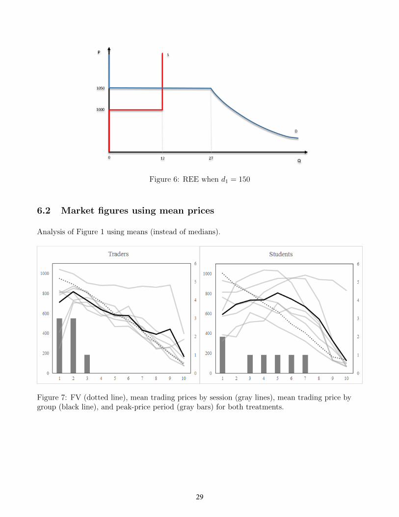
Figure 6: REE when d1 = 150

6.2 Market figures using mean prices

Analysis of Figure 1 using means (instead of medians).

Figure 7: FV (dotted line), mean trading prices by session (gray lines), mean trading price bygroup (black line), and peak-price period (gray bars) for both treatments.

29

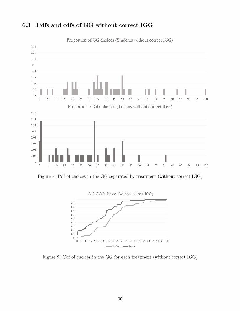
6.3 Pdfs and cdfs of GG without correct IGG

Figure 8: Pdf of choices in the GG separated by treatment (without correct IGG)

Figure 9: Cdf of choices in the GG for each treatment (without correct IGG)

30

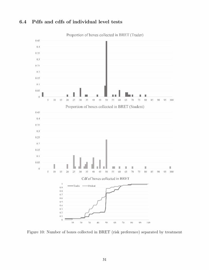
6.4 Pdfs and cdfs of individual level tests

Figure 10: Number of boxes collected in BRET (risk preference) separated by treatment

31

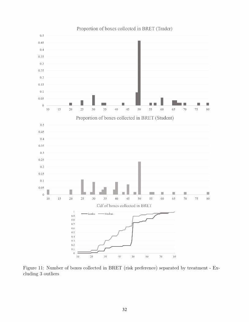
Figure 11: Number of boxes collected in BRET (risk preference) separated by treatment - Ex-cluding 3 outliers

32

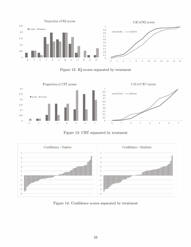
Figure 12: IQ scores separated by treatment

Figure 13: CRT separated by treatment

Figure 14: Confidence scores separated by treatment

33

6.5 Bomb Risk Elicitation Task (BRET)

34

35

6.6 Guessing Game Screen Shot

36

6.7 Individual Guessing Game Screen Shot

37

6.8 Raven’s Test Instructions

Station #__________________

Please do not turn the page until you are instructed to do so

This is a test of observation and clear thinking. It will involve answering problems such as C3 below. The

top part of problem C3 shows a pattern with a piece cut out of it. Look at the pattern, think what piece is

needed to complete the pattern correctly both along the rows and down the columns must be like. Then find

the right piece out of the 8 pieces shown below. Number 3 is the right piece, isn’t it? To submit that your

answer is Number 3, you will need to circle the Number 3 piece.

On every page of this booklet there is a pattern with a piece missing. You have to choose which piece is the

right one to complete the pattern. When you think you have found the right piece, circle it on your booklet

and move onto the next page. If you make a mistake, or want to change your answer, put a cross through the

incorrect answer, and circle your correct answer. You will have 10 minutes to complete all 18 pages of this

booklet. When everyone is ready, the experimenter will let you begin and start the timer. The experimenter

will announce when 10 minutes is finished and, at that time, you will need to stop working and put down

your pen.

38

6.9 CRT

(1) In a lake, there is a patch of lily pads. Every day, the patch doubles in size. If it takes 48 days for thepatch to cover the entire lake, how long would it take for the patch to cover half of the lake? ____ days

(2) If it takes 5 machines 5 minutes to make 5 widgets, how long would it take 100 machines to make 100widgets? ____ minutes

(3) A bat and a ball cost £1.10 in total. The bat costs one pound more than the ball. How much does the ballcost? ____ pence

(4) If John can drink one barrel of water in 6 days, and Mary can drink one barrel of water in 12 days, howlong would it take them to drink one barrel of water together? _____ days

(5) Jerry received both the 15th highest and the 15th lowest mark in the class. How many students are in theclass? ______ students

(6) A man buys a pig for £60, sells it for £70, buys it back for £80, and sells it finally for £90. How muchhas he made? _____ dollars

(7) Simon decided to invest $8,000 in the stock market one day early in 2008. Six months after he invested,on July 17, the stocks he had purchased were down 50%. Fortunately for Simon, from July 17 to October 17,the stocks he had purchased went up 75%. At this point, which statement is true? (Circle the correct answer)

a. Simon has broken even in the stock market

b. Simon is ahead of where he began

c. Simon has lost money

39

6.10 Confidence Instructions

40

6.11 Occupation questions (Traders only)

Occupational Characteristics

In which type of financial institution do you work?

Investment bank (please specify if capital market or investment banking

division)____________

Investment fund

Private equity fund

Other (e.g., commercial bank) ________________________________________

In your current (or past) employment do (did) you operate directly on financial markets (as a

trader or portfolio manager)? _______________________

Yes

No

What percentage of your typical working day do you spend on the following tasks?

A) Trading on financial markets __________________________________

B) Following the financial markets in real time? _______________________________________

Which of these categories best describe your job:

Trader

Proprietary trader

Portfolio manager

Sales-trader

Sales with management of virtual portfolios (e.g. alpha capture)

Sales without

Macro-analyst

Equity/credit analyst

Other: _______________________________________________________________

Briefly describe your job.

______________________________________________________________________________

______________________________________________________________________________

______________________________________________________________________________

For how many years have you worked in the financial industry? __________________________

Demographic Characteristics

What is your age? (You can leave this blank if you prefer not to say) ______________________

Your education: (E.g., BSc Econ and MSc Engineering) ________________________________

What is your gender?

Male

Female

Prefer not to say

41

6.12 Call for subjects (Traders only)

CENTRE FOR FINANCE

www.centreforfinance.org

Laboratory Experiments on Financial Decision Making at UCL

Call for Participants

The Centre for Finance at UCL is running a series of laboratory experiments on financial

decision making. We will run two experiments with financial professionals.

For Experiment 1, we need participants who are either traders or portfolio managers or who

have had such roles in the past. You are also eligible if you do not have the formal title of trader

or portfolio managers, but you perform activities that are closely related to that of a trader or

portfolio manager (e.g., sales-trader or sales on the trading floor).

For Experiment 2, we need participants from a broader class of financial professionals. You

are eligible to participate in Experiment 2 if you are currently working in the core business of

a financial institution, e.g., as a trader, analyst, sales person, economist, investment banker.

In the study, participants will first read some instructions and then will be asked to make some

decisions (e.g., trade a fictitious asset according to a simple trading protocol). We anticipate

that participants will earn an average of £200; the precise amount that a participant will

make depends on his or her own decisions, the decisions of others and some randomness.

To help us in this study, participants must come to our laboratory only once, for two hours, on

a pre-specified date and time. Our laboratory is located in Bloomsbury, close to Euston Station

(Drayton House, 30 Gordon Street, WC1H 0AX – Map).

At this stage we only need a general expression of interest. Please email the Centre for

Finance’s laboratory at elfe.experiments@ucl.ac.uk as soon as possible indicating your interest

in participating. In the subject line of your email, please type either “CFF Experiment 1” or

“CFF Experiment 2”. In the body of your email, please type your current job position and your

name. No other text is required. If you are not sure about your eligibility for Experiment 1,

indicate “CFF Experiment”. We will contact you with details in the next few days.

The precise dates and times will be decided after coordinating with the participants. We plan

to run the experiment in a series of sessions in the period of November 2018 – February 2019.

You will be asked to participate in one session and you will have the opportunity to choose the

date and time that better suits you. The experiment sessions will be conducted on weekdays

after business hours or on the weekend.

Participating in the experiment will be fun. We will not use any physically invasive procedures.

Experiments in our laboratory respect all the regulations for activities with human subjects. In

particular, participants are guaranteed anonymity, and the data collected will remain strictly

confidential. The names of participants or of their institutions will not be published or

revealed anywhere. The protocol in the laboratory assures that even those running the

experiment are not able to link the behaviour and choices made in the laboratory to a

particular individual.

We thank everyone interested in advance.

Antonio Guarino

Professor of Economics, Department of Economics, UCL

Director, Centre for Finance, UCL

Email: a.guarino@ucl.ac.uk

42

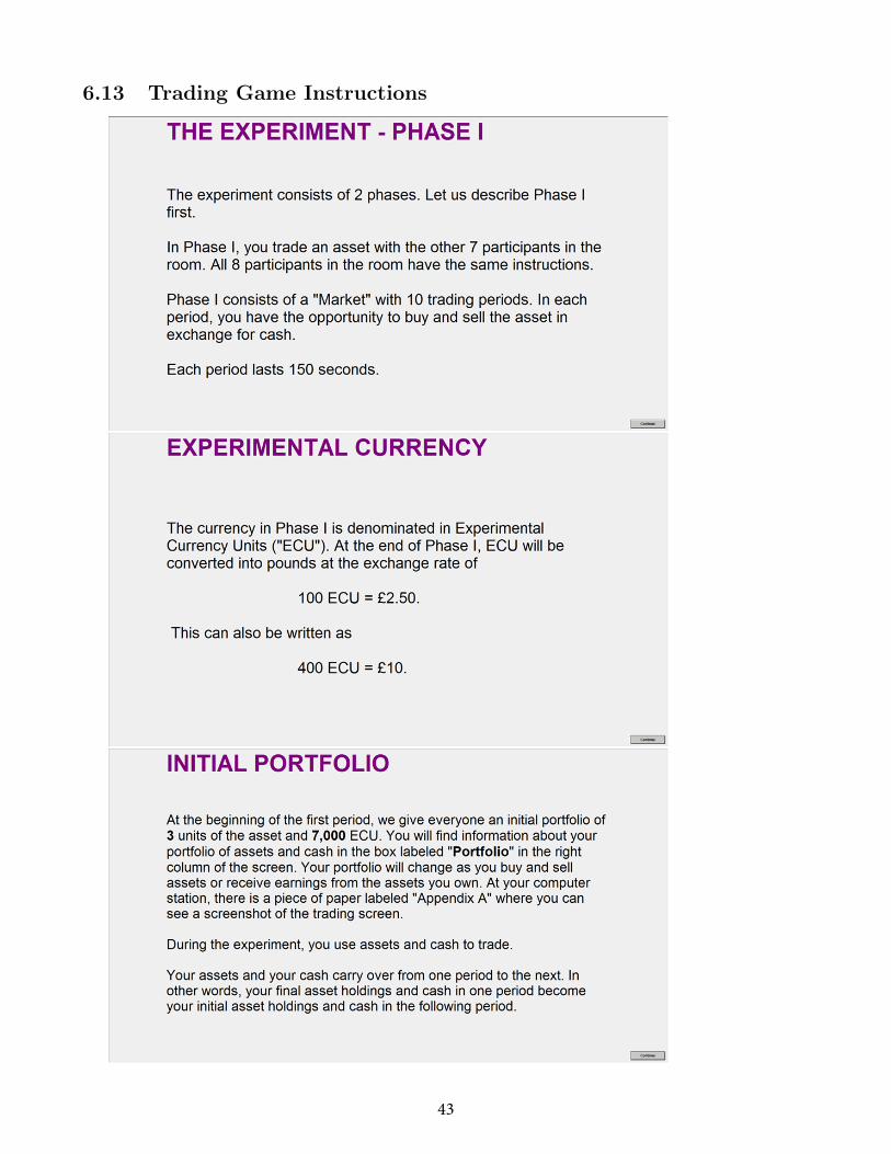
6.13 Trading Game Instructions

43

44

45

46

47

48

49

50

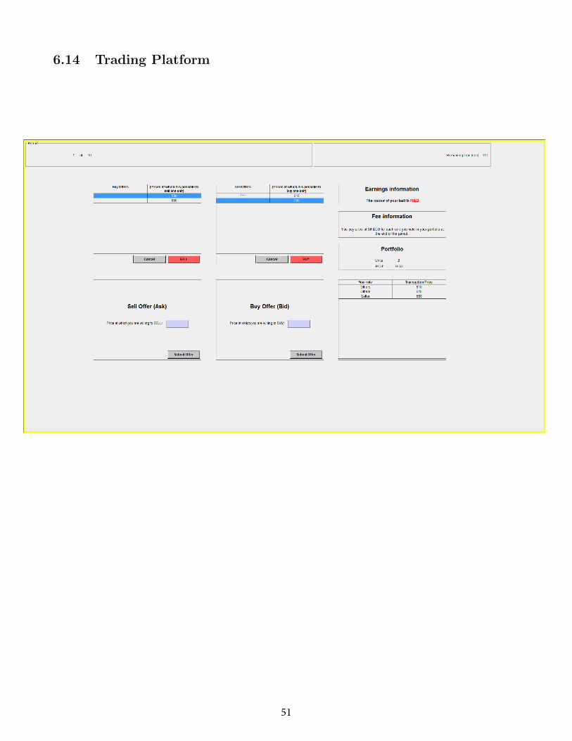
6.14 Trading Platform

51