Trade Patterns in a Globalised World: The Case of Brazil · André Nassif Department of Economics,...
83
Texto para Discussão 012 | 2018 Discussion Paper 012 | 2018 Trade Patterns in a Globalised World: The Case of Brazil André Nassif Department of Economics, Fluminense Federal University, Brazil [email protected] Marta dos Reis Castilho Institute of Economics, Federal University of Rio de Janeiro, Brazil [email protected] This paper can be downloaded without charge from http://www.ie.ufrj.br/index.php/index-publicacoes/textos-para-discussao
Transcript of Trade Patterns in a Globalised World: The Case of Brazil · André Nassif Department of Economics,...

Texto para Discussão 012 | 2018
Discussion Paper 012 | 2018
Trade Patterns in a Globalised World: The Case of Brazil
André Nassif Department of Economics, Fluminense Federal University, Brazil
Marta dos Reis Castilho Institute of Economics, Federal University of Rio de Janeiro, Brazil
This paper can be downloaded without charge from
http://www.ie.ufrj.br/index.php/index-publicacoes/textos-para-discussao
IE-UFRJ DISCUSSION PAPER: NASSIF; CASTILHO, TD 012 - 2018. 2
Trade Patterns in a Globalised World:
The Case of Brazil September, 2018
André Nassif Department of Economics, Fluminense Federal University, Brazil
Marta dos Reis Castilho Institute of Economics, Federal University of Rio de Janeiro, Brazil
Paper prepared for 21st FMM (Forum for Macroeconomics and Macroeconomic Policies) Conference:
“The Crisis of Globalisation” in Berlin, Germany, 9-11 November, 2017, and the 3rd Iberoamerican
Socioeconomic Meeting of SASE (Society for the Advancement of Socioeconomics) in Cartagenas de
Indias, Colombia, 16-18 November, 2017. The first draft of this paper was prepared when one of its authors
(André Nassif) still worked at BNDES as a professional economist. He retired from BNDES in December,
2016. The authors thank Filipe Lage de Souza for helpful comments and suggestions.
IE-UFRJ DISCUSSION PAPER: NASSIF; CASTILHO, TD 012 - 2018. 3
Abstract
Globalisation can be defined as the extent and intensity with which a country’s production, trade and capital flows are integrated in the world economy. Our focus is on the globalisation through international trade flows. After analyzing the main theoretical predictions about the effects of global trade integration on trade patterns between countries of different levels of income and technology, this paper investigates the case of Brazil, focusing on its trade integration over the last 26 years (1990-2016). Particularly, we are interested in investigating whether or not (and if so, to what extent) Brazil’s recent trajectory has been directed to a regressive pattern of specialisation. By regressive specialisation we refer to that in which both production and export structures are strongly oriented to goods of low technological sophistication and low income-elasticity of demand. The recent theoretical literature on technological gaps and long-term growth suggests that when a country enters into a quick and sustained regressive pattern of specialisation, its capacity of showing growth rates aligned with its balance-of-payment equilibrium is reduced and, therefore, a falling behind trajectory is observed. Our main empirical findings are (i) the technological gap significantly widened for all groups of manufactured goods classified by factor content and technological sophistication; (ii) the income elasticity of demand for Brazilian exports is greater than for Brazilian imports, suggesting a regressive specialisation concentrated in low-tech goods and implying that growth has been constrained by long-term balance-of-payments equilibrium (Thirlwall’s law); and (iii) a very marked trend of high concentration of Brazilian exports in primary goods, but a more diversified basket of imports composed of high technologically sophisticated manufactured goods, reinforcing the regressive specialisation of Brazil’s trade pattern in the last decades.
Keywords: patterns of specialisation; regressive specialisation; diversification; Brazil
JEL Classification: F10; F11; F12; F14.

IE-UFRJ DISCUSSION PAPER: NASSIF; CASTILHO, TD 012 - 2018. 4
Summary
Abstract ............................................................................................................................... 3
1 INTRODUCTION ....................................................................................................................................................... 5
2 TRADE PATTERNS IN A GLOBALISED WORLD: A SURVEY OF THE THEORETICAL LITERATURE .......... 8
2.1 Trade patterns in traditional trade models of comparative advantage ........................... 8
2.2 From the heterodox models of the 1960s to the “new trade theories” of the late 1970s
and onwards ........................................................................................................................... 14
2.2.1 Linder’s demand-push trade model and the “new trade theories” of the late 1970s
and onwards ....................................................................................................................... 14
2.2.2 The “new new trade theories” of intrafirm global trade and theoretical models
explaining the genesis of global value chains .................................................................... 19
2.3 A Structuralist-Neoschumpeterian technological gap model: trade patterns and growth
dynamics ................................................................................................................................ 23
3 EMPIRICAL EVIDENCE: THE CASE OF BRAZIL ............................................................................................... 34
3.1 A brief analysis on Brazil’s economic reforms and some previous indicators (1990-
2017) 34
3.2 Brazil’s trade patterns and the recent trajectory towards regressive specialisation ..... 45
4 CONCLUDING REMARKS ..................................................................................................................................... 64
REFERENCES ................................................................................................................................................................ 66
APPENDIX 1 .................................................................................................................................................................. 76
Classification of Brazilian Industries according to Factor Content and Technological
Sophistication (Correspondence between STIC Revision 2 and Pavitt’s taxonomy).............. 76
APPENDIX 2 .................................................................................................................................................................. 82
Trade Indicators ..................................................................................................................... 82

IE-UFRJ DISCUSSION PAPER: NASSIF; CASTILHO, TD 012 - 2018. 5
1 Introduction
Globalisation can be defined as the extent and intensity with which a country is integrated
in the world economy. Although such integration can and does reach production, trade
and capital flows, our focus is on the globalisation through international trade flows.
Although other earlier waves of economic internationalisation have happened—from the
Industrial Revolution till the beginning of World War I—, the speed and intensity with
which the present wave of trade globalisation has spread over the entire world economy
since the early 1980s has no precedent in the modern occidental economic history. In fact,
from the 1980s onwards, the rise and diffusion of the microelectronic revolution as well
as the significant reduction of trade barriers also put pressure on most developing
countries to accelerate trade integration into the world economy.
In the case of Brazil, for instance, between 1990 and 1994, after several decades of
protectionist policies adopted under the import substitution development strategy, the
Brazilian government decide to adopt a unilateral and ambitious trade liberalisation
programme, which eliminated most non-trade barriers and reduced average nominal
tariffs for all goods from 30.5% to 11.2%.1 Since several studies were released in the
1990s and 2000s with the goal of evaluating the impacts of the Brazilian trade
liberalisation experience on productivity, trade pattern, employment, etc.,2 this paper does
not aim at replicating such studies. However, there is extensive literature documenting
that two marked phenomena have characterised the Brazilian economy in the last 25
years: the first one is the significant and continuous reduction of the share of value-added
industrial activities in the GDP;3 and the second one is a recurrent long-term trend of
overvaluation of the Brazilian currency in relation to the currencies of Brazil’s main
trading partners.4 Although the second phenomenon may have contributed to deepening
the first one, both may have influenced the observed changes in the pattern of trade
1 See Kume, Piani and Souza (2000:11).
2 See Feijó and Carvalho (1994), Moreira and Correa (1998), Bonelli and Fonseca (1998), and Nassif
(2003).
3 See Nassif (2008), Oreiro and Feijó (2010) and Nassif, Feijó and Araújo (2015), among others.
4 See Bresser-Pereira (2010), Nassif, Feijó and Araújo (2017) and Nassif, Bresser-Pereira and Feijó (2017).

IE-UFRJ DISCUSSION PAPER: NASSIF; CASTILHO, TD 012 - 2018. 6
integration of the Brazilian economy in terms of sectoral specialisation, geographical
composition of trade flows and the competitiveness of Brazilian goods.
This paper has two main goals: first, it reviews and analyzes the main theoretical
predictions about the effects of global trade integration on trade patterns between
countries of different income and technological levels; and second, it investigates the case
of Brazilian trade integration over the last 26 years (1990-2016). Particularly, we are
interested in investigating whether or not (and if so, to what extent) Brazil’s recent
trajectory has been directed to a regressive pattern of specialisation. By regressive
specialisation we refer to that in which both production and export structures are strongly
oriented to activities or segments of low technological sophistication and low income
elasticity of demand.5 As we will further discuss, the recent theoretical literature on
technological gaps and long-term growth suggests that when a country enters into a quick
and sustained regressive pattern of specialisation, its capacity of showing growth rates
aligned with their balance-of-payment equilibrium is reduced and, therefore, it enters a
“falling behind” trajectory, the term coined by Abramovitz (1986) to contrast with a
“catching up” path.
For analyzing Brazil’s recent change in trade patterns, we will estimate the following
indicators: (i) income elasticity of demand for exports and imports; (ii) the composition
and dynamics of both exports and imports classified by factor content and degree of
technological sophistication; (iii) the degree of export diversification and the importance
of the extensive and intensive margins of trade for Brazilian exports, whose indicators
permit us to measure the extent to which Brazil’s export expansion resulted from the
expansion of “old” (intensive margin) or “new” (extensive margin) products; iv) the
degree of concentration versus diversification of the export basket; v) the index of
intraindustrial trade; and vi) the geographical distribution of exports and imports. Most
5 Coutinho (1997) first coined the term regressive specialisation when analysing the Brazilian economy
throughout the 1990s. In our paper, rather than production, we will emphasise the trade (export and import)
structures.
IE-UFRJ DISCUSSION PAPER: NASSIF; CASTILHO, TD 012 - 2018. 7
indicators will be calculated through descriptive statistics, using a methodology compiled
by Reis and Farole (2012).
The paper is divided into 4 sections, including the Introduction. Section 2 presents a
theoretical analysis of the determination of trade patterns in a globalised economy,
emphasising recent theories of international trade and focusing on trade flows between
countries with different per capita income and technological levels. Section 3 presents a
general view of the Brazilian economy during the period under study and shows empirical
evidence of Brazil’s recent experience, based on the above-mentioned indicators. Section
4 draws the main conclusions of the study as well as suggesting some policy implications.

IE-UFRJ DISCUSSION PAPER: NASSIF; CASTILHO, TD 012 - 2018. 8
2 Trade patterns in a globalised world: a survey of the theoretical literature
2.1 Trade patterns in traditional trade models of comparative
advantage
The investigation of the determinants of trade patterns and the advantages of a country to
engage in global trade has been a long tradition in economics. In the classical political
economy, technological capacity was the main source for explaining different sectoral
productivity levels between countries and, therefore, the existence of global trade. Adam
Smith (1776), however, was more worried about the effects of global trade on a country’s
economic growth, while David Ricardo (1817) and John Stuart Mill (1848) deviated
completely from the theoretical analysis to the effects of international trade on the
allocative efficiency of productive resources and its capacity to increase social well-being
by augmenting the trade volume between countries engaged in free trade. Indeed, in
Smith’s theoretical analysis, trade was driven by differences in sectoral absolute costs
between countries (which reflect, in turn, differences of absolute technology and
productivity), whereas in Ricardo’s and Mill’s analysis, trade was driven by differences
in sectoral relative costs (which reflect, in turn, differences of comparative productivity).
Since in Ricardo’s and Mill’s theoretical framework technology was exogenously
determined and evaluated in comparative terms, they started a long-lasting tradition in
which trade patterns were basically determined by supply-side forces.
In the modern neoclassical theoretical treatment of Ricardian analysis, the determination
of trade pattern by comparative advantage depends on several unrealistic assumptions,
such as perfect competition in goods and labour markets, total domestic labour mobility,
technologies subject to constant returns to scale and full employment. Under such
conditions, by extending the analysis to many goods (a continuum of goods), Dornbusch,
Fischer and Samuelson’s (1977) seminal paper showed that comparative advantage and
trade pattern are jointly determined by different relative productivities at the sectoral level
and different relative wages between countries. In fact, since differences in sectoral
relative productivities are determined first and ranked for each country, and given a
country’s relative wage compared with another trade partner, it is possible to determine
the range of goods in which each one of them has comparative advantage. As the

IE-UFRJ DISCUSSION PAPER: NASSIF; CASTILHO, TD 012 - 2018. 9
expenditure shares are the same in both trade partners (homothetic demand), the demand
side has no role in determining trade pattern. In such circumstances, international trade
leads to complete interindustrial specialisation, even considering that a subset of goods
cannot eventually be traded, be it because relative unit labour costs (that is, the ratio of
wage rates to labour productivity) are the same in both countries, or because transport
costs can be high enough to work as a trade constraint.
Although the Ricardian hypothesis for determining a country’s trade pattern (different
sectoral relative productivities reflecting distinct relative technologies) has been
supported by several empirical tests,6 it was the Heckscher-Ohlin (H-O) version of
comparative advantage that became the standard neoclassical trade model for explaining
trade pattern, gains from trade and advantages of free trade policies. In fact, in an original
paper written when Sweden was still a net export of agricultural goods, Eli Heckscher
(1919) argued that, in a world characterised by different relative factor endowments, each
country tends to specialise in the production of goods intensively using the abundant
factor, importing goods that intensively use the scarce factor. In a doctoral thesis
supervised by Heckscher, Bertil Ohlin (1924) transformed those original views into an
elegant mathematical framework that not only permitted the determination of a unique
solution for the trade pattern, but also the establishment of a theoretical basis for
developing a set of important theorems about global trade by neoclassical economists.
The original model proposed by Ohlin (1924) is based on the following set of
assumptions: (i) the technology of each industry i, subject to constant returns to scale, is
the same for all countries in the world; (ii) there is no possibility of factor-reversal (that
is, the technology cannot be reversed by changes in factor prices); (iii) each country
(“region”, in Ohlin’s word) is defined by its relative factor endowment; (iv) each factor
of production has perfect domestic mobility; (v) relative abundance or scarcity of each
factor of production defines its relative price in autarky; and (vi) given production
functions and preferences, each country has its relative goods and factor prices, output
and resources allocation determined by the Walrasian general equilibrium mechanisms.
6 See McDougall (1951) and Eaton and Kortum (2002).
IE-UFRJ DISCUSSION PAPER: NASSIF; CASTILHO, TD 012 - 2018. 10
The main proposition of the H-O model is that each country exports goods that intensively
use the abundant factor in their production, and imports those that intensively use the
scarce factor.
In his book “Interregional and International Trade”, Ohlin (1933) showed that, if the
world economy was characterised by industries that operate under perfect competition
and factor immobility, free trade—by changing relative factor prices in each country—
would be the main channel explaining geographical location of productive activities and
pattern of specialisation. It is worth noting that, in the H-O model, the unrealistic
assumption of identical and unchanged sectoral technologies between countries is kept
even when relative factor prices are changed by free global trade. In a word, trade is the
main channel through which each country can surpass the scarcity of some factors of
production.
The original presentation of the H-O model in a Walrasian general equilibrium framework
eased the development of important theorems related to free trade. The first one, shown
by Samuelson (1948; 1949), is the factor price equalisation theorem, which predicts that,
under a set of restricted conditions, such as perfect competition in goods and factors
markets (in a model of two sectors and two factors), homothetic demand and trade
completely determined by the H-O proposition, free trade integration tends to generate a
total equalisation of goods and factor prices since both goods will be produced by both
countries. The intuition of this theorem is simple: since a country can use more than one
factor (say, capital and labour, and not only one factor, as in the Ricardian model), trade
in goods generates a full equalisation of factor prices through full equalisation of goods
prices.7 As Feenstra (2004: 13) points out, the factor equalisation theorem suggests that
“trade in goods is a perfect substitute for trade in factors”. In the face of large inequality
in wages between countries in the global economy, the theorem has a very unrealistic
conclusion. However, it demonstrates that free global trade generates, at least, changes in
relative goods and factor prices compared with those observed in autarkic conditions.
7 For an original mathematical demonstration, see Samuelson (1949), and for a rigorous recent
demonstration, see Feenstra (2004:13-15).
IE-UFRJ DISCUSSION PAPER: NASSIF; CASTILHO, TD 012 - 2018. 11
The second theorem, demonstrated by Stolper and Samuelson (1941), shows that if
comparative advantage is the main force to govern trade patterns in the global economy,
free trade can predict net gains for society as a whole in each country, but its impacts on
income distribution is unequal among the factors of the owners of production. The
intuition of this theorem is also quite simple: it says that, if two goods are produced under
constant returns to scale and perfect competitive conditions in a country, the engagement
in free trade relations tends to increase the relative price of the exported good and,
therefore, to also increase the relative price of the factor intensively used in its
production; but tends to decrease the relative price of the imported good as well as the
relative price of the factor intensively used in its production. In a word, the Stolper-
Samuelson theorem shows that free trade redistributes the national income to the owners
of the abundant factor in such a way that the main losers are the owners of the scarce
factor.
It is curious that most studies based on the H-O model do not worry about the eventual
effects of technological change on a country’s trade pattern. If technical progress occurs,
it is always an exogenous phenomenon. The same cannot be said about changes in a
country’s endowment. In this case, as the third theorem derived from the H-O model
stresses (the Rybczynski theorem), a change in factor endowment of a country will change
the relative output of the economy. Rybczynski (1955) supposes two factors (say, natural
resources and labour) and two industries (one natural resource-based, and the other,
labour intensive) subject to constant returns to scale and perfectly competitive. If new
large sources of natural resources are discovered in a country, there will be a
disproportional rise in the output of the natural resource-based sector and a contraction of
the labour intensive. This result depends on the relative factor prices remaining
unchanged, a requirement that is easily satisfied because the relative demand of the
factors is going in opposite directions (while demand of natural resources is increased,
the demand of labour is contracted proportionally).
It is important to remember that the normative implications of the H-O model and the
factor price equalisation theorem were severely criticised by Latin American economists
in the early 1950s. The most severe attack came from Raúl Prebisch, the first executive
secretary of the United Nations Economic Commission for Latin America and the
IE-UFRJ DISCUSSION PAPER: NASSIF; CASTILHO, TD 012 - 2018. 12
Caribbean (ECLAC). In an influential paper, Prebisch (1950) criticised the main
hypothesis that supports the equalisation factor price theorem: first, while the theorem
predicts that the engagement of primary products exporting countries in free global trade
would favour relative prices and industrialisation by importing capital goods with falling
relative prices, Prebisch (1950) argued that such a result depends on the income elasticity
of demand of both goods being equal to one, a hypothesis not held in practice;8 and
second, as empirical evidence shows that manufactured goods (the main imported good
of Latin American countries) have much higher income elasticity of demand in the long
run, periphery countries specialised in primary and commodity goods have their long-
term economic growth recurrently constrained by balance of payments crisis.9 10
Indeed, the soundness of the H-O model as a general theoretical approach to explain trade
patterns and gains from trade has long lived up to theoretical and empirical proofs. The
theoretical model was originally developed for two sectors, two factors and two countries
(2x2x2 model). However, if we consider an extended H-O model including many goods,
many factors and many countries, the determination of the trade pattern becomes quite
complicated. Several studies have shown that the trade pattern, the factor price
equalisation and the Stolper-Samuelson theorem are only rigorously determined if the
number of goods, factors and countries is equal. In the more realistic case in which the
number of goods is higher than the number of factors (maintaining two trade countries),
the trade pattern is indeterminate (Feenstra, 2004: 65).
8 In Prebisch’s (1950:1, italics ours) words, “it is true that the reasoning on the economic advantages of the
international division of labour is theoretically sound, but it is usually forgotten that it is based upon an
assumption which has been conclusively proved false by facts. According to this assumption, the benefits
of technical progress tend to be distributed alike over the whole community, either by the lowering of prices
or the corresponding raising of incomes”.
9 As Thirlwall (2011:13) recognized, Prebisch’s (1950) equation expressing his centre-periphery model was
“the true forerunner of my [that is, Thirlwall’s] balance of payments constrained growth model developed
much later”.
10 Needless to say, Prebisch’s (1950) criticism was related to the long-term trend (or secular trend) of the
income elasticity of demand of manufactured goods vis-à-vis primary and commodity goods. In other
words, rather than static gains from trade, Prebisch was worried about the dynamic effects on economic
development for countries unconditionally engaged in free global trade and specialised in primary goods.
IE-UFRJ DISCUSSION PAPER: NASSIF; CASTILHO, TD 012 - 2018. 13
At the empirical level, the most controversial result was the famous Leontief’s (1953) test
which, by calculating the capital/labour ratio for US exports and imports for 1947, showed
that the share of US exports was mostly labour-intensive. Since the US was then
considered a capital abundant country, the Leontief paradox revealed the theoretical
inability of the H-O model to explain the country’s trade pattern. Since Leontief’s (1953)
test was published, the H-O model has been subjected to a continuing debate between
Neoclassical and Structuralist economists. Within the Neoclassical framework, the first
discussions concentrated on possible explanations for Leontief test not to validate the H-
O predictions, such as having ignored other factors of production (e.g., land) not capital
and labour and not having considered skilled and unskilled labour. At the empirical level,
since the original H-O model did not take into consideration such a hypothesis, this kind
of criticism is misleading (Feenstra, 2004: 37).
Since then, empirical tests on the main predictions of the H-0 model have used the
procedure suggested by Vanek (1968), according to which, instead of the capital-labour
ratio of exports and imports, as in Leontief’s test, the test should estimate the factor
content of exports as well as the factor content of imports. Through input-output matrices,
he suggests computing the factor service content in each exported and imported good. For
instance, an estimate of Brazil’s net exports (calculated as the difference between the
domestic output and domestic consumption) results in the difference between the factor
content of its exports and the factor content of its imports. If the difference is positive, it
means that Brazil exports (on net) the services of this input; if the difference is negative,
it means that Brazil imports (on net) the services of this input. The Heckscher-Ohlin-
Vanek (H-O-V) model is appealing for permitting friendlier empirical tests on trade
pattern based on the factor proportion model. However, the Vanek (1968) model requires
several restricted assumptions, such as identical constant-returns-to-scale technologies
for all countries in the world and total factor price equalisation. Despite this, the modern
acceptance of factor proportion theory is considered within the H-O-V framework.11
11 See, for instance, Helpman and Krugman (1985, ch.1) and Feenstra (2004: 37-56) for mathematical
demonstrations. See Helpman (2011:38-45) for textual presentation.

IE-UFRJ DISCUSSION PAPER: NASSIF; CASTILHO, TD 012 - 2018. 14
As to Structuralist criticisms on the H-O model, the Leontief paradox gave rise to several
academic studies in the 1960s aiming at investigating new hypotheses for explaining trade
patterns in the manufacturing sector as well as the dynamic effects of free global trade on
long-term growth. This will be discussed in the following subsections.
2.2 From the heterodox models of the 1960s to the “new trade
theories” of the late 1970s and onwards
2.2.1 Linder’s demand-push trade model and the “new trade theories” of the late
1970s and onwards
The so-called “new trade theory”, a modern theoretical current of international trade
captained by Paul Krugman, Elhanam Helpman, Anthony Venables, James Brander,
Barbara Spencer and others, justifies the adjective “new” because most models
incorporate imperfect competition, increasing returns to scale and the dichotomy of
homogeneous versus differentiated goods as basic assumptions. However, such
assumptions had been considered by heterodox authors in the 1960s, like Staffan Linder
(1961), Michael Posner (1961) and Raymond Vernon (1966). Indeed, differently from the
former group of authors, this latter group, as they did not construct formal trade models,
treated forces such as oligopolistic or monopolistic competition, product differentiation
and economies of scale more as possibilities than precise hypotheses. Even so, the major
innovation of some of these models pioneered a demand basis trade theory for explaining
a country’s international competitiveness for exporting manufactured goods. In this
subsection, we will only present the Linder (1961) model.
Linder (1961) accepts the theoretical hypothesis of factor endowment for explaining
international trade of natural resources-based goods (especially agricultural goods).
However, he rejected the H-O model in the explanation of international trade in
manufactured goods. His model is one of the first to emphasise the central role of
domestic market size in providing demand high enough for creating potential
international competitiveness for a country to export manufactured goods. Like under free
trade, the initial costs are high enough for firms of the manufacturing sector to export. As
a matter of fact, Linder (1961) stresses that a “representative demand” must exist in the
domestic market before the global markets can be reached. In other words, as most
industrial firms of the manufacturing sector have to choose technologies subject to
IE-UFRJ DISCUSSION PAPER: NASSIF; CASTILHO, TD 012 - 2018. 15
increasing returns to scale, they will not be able to have international competitiveness for
exporting such goods if the size of the domestic market is not large enough to provide
them minimum efficient scales. For Linder, then by taking advantage of their proximity
to their respective domestic markets, firms seek to explore economies of scale in order to
reach foreign markets in the future. In Linder’s (1961) theoretical model, the higher a
country’s per capita income, the higher will be the size of its domestic demand and the
more sophisticated will be the demand pattern. Thus, its potential for exporting
manufactured goods will be higher. His main conclusion is that countries with the highest
and closest levels of per capita income have a significant share of their manufacturing
trade characterised by intraindustrial trade of differentiated goods. The importance of
Linder’s theoretical model is that he was the first to explain the predominance of
manufactured goods in the trade among countries of similar per capita income. His main
contribution is that he was the first to not only indicate economies of scale and product
differentiation as the main sources of intraindustrial global trade, but also to suggest that
such sources are primarily realised in the domestic marketplace, before firms are able to
compete in the global markets.12
Yet, from the late 1970s on, a set of neoclassical models labelled by Krugman (1990) as
“new trade theory” began to appear. Rather than for having incorporated imperfect
competition, the adjective “new” can be justified by three main reasons:
i) First, because these models demonstrated that, in certain oligopolistic cases,
as trade pattern depends on a combination of complex factors existing in each
country, such as market size, number of competing firms, factor prices,
barriers to entry, etc., its theoretical determination is much harder to predict;
in some cases, the trade pattern is either undetermined (see Helpman and
12 It is unacceptable that Linder’s (1961) contribution, despite being recognized by Krugman’s (1979)
seminal paper, has been omitted from the bibliographic references in Krugman, Obstfeld and Melitz (2012),
Helpman and Krugman (1985) and Feenstra (2004), the three leading textbooks in undergraduate and
graduate courses.
IE-UFRJ DISCUSSION PAPER: NASSIF; CASTILHO, TD 012 - 2018. 16
Krugman, 1985: 86-88) or presents multiple equilibria (see Helpman and
Krugman, 1985: 53-55);
ii) Second, because these authors mathematically demonstrated the original
Graham’s (1923) conjecture according to which, in the presence of economies
of scale and market power, trade globalisation can, under certain conditions,
lead to an unequal distribution of gains among countries. If for example, trade
reallocates productive resources from sectors subject to increasing returns to
scale to sectors subject to constant returns to scale in a country, all gains from
trade may be appropriated by the countries whose reallocation of resources
happened in the opposite way (see Helpman and Krugman, 1985: 50-55);
iii) And third, because, by using Vanek’s (1968) suggestion of estimating the
trade pattern based on the factor content services presented in both exports
and imports, these models also seek to show how the basic H-O-V model can
interact with new models incorporating economies of scale, product
differentiation and monopolistic competition.
In this section, as we are interested in cases in which the trade pattern can be determined
and the gains from trade are assured for all countries, the new trade theory shows that
such cases are only guaranteed if imperfect competition assumes the monopolistic
competition form.13 In the basic model presented by Krugman (1979, 1980), an industry
from two countries is composed of several firms producing a large number of
differentiated goods and competing in monopolistic competition. Despite all firms using
only one factor of production (labour), as technology is identical for all firms, but subject
to economies of scale, and all differentiated products enter symmetrically into demand,
each firm produces only one differentiated and close substitute good. As competition is
driven by product differentiation, each firm chooses its price and maximizes profits by
13 We leave the cases in which the presence of increasing returns to scale makes a country reduce its social
well-being and long-term growth after engaging in free trade for the next section.
IE-UFRJ DISCUSSION PAPER: NASSIF; CASTILHO, TD 012 - 2018. 17
equalising marginal revenue to marginal cost, but ignoring the prices fixed by their
competitors in the market.
To demonstrate that the economies of scale are the main cause for trading, Krugman
(1980) also supposes that both countries have the same factor endowments and
technological level. Considering zero transport costs, if these countries decide to engage
in free trade, rather than being driven by any difference between relative costs or factor
endowments (as in traditional models of comparative advantage), trade pattern will be
determined by economies of scale and product differentiation, in such a way that each
differentiated good is produced by only one firm and in only one country.14 Differently
from comparative advantage, in which trade pattern is of the interindustrial type, trade
pattern driven by economies of scale and product differentiation is of the intraindustrial
type. As Krugman (1980: 952) concludes, “gains from trade will occur because the world
economy will produce a greater variety of goods than would either country alone, offering
each individual a wider range of choice”. Even though the direction of trade is
undetermined, since all range of goods are differentiated, it does not matter who produces
what, but rather that trade integration provides a greater volume of varied goods. In an
extended model, Krugman (1980) also considers the case in which one of the two
countries has a larger domestic market than the other. The result is as intuitively expected:
since a larger domestic market has a major potential for exploring economies of scale, the
bigger country will be a net exporter of all range of goods whose technology is subject to
increasing returns to scale, as had already been suggested by Linder (1961).
14 The introduction of transport costs does not modify the general results. See Krugman (1980, section II:
953-955).

IE-UFRJ DISCUSSION PAPER: NASSIF; CASTILHO, TD 012 - 2018. 18
Figure 1: Global trade between developed and developing countries
Source: Elaborated by the authors, based on Krugman (1990:77)
In another paper, Krugman (1981) integrated the traditional Heckscher-Ohlin trade model
with the main features of the new trade theory, whose results are illustrated in Figure 1.
With this paper, Krugman completed the trilogy that might have justified his Nobel Prize
laureate in 2008.15 Krugman (1981) proposed a model in which the global economy is
composed of several countries defined by either their similarity or differences in their
factor endowments.16 In practical terms, if we divide this world into two groups of
countries, the first would be formed by all capital-abundant developed countries, while
the second would be composed of all natural-resources-abundant developing countries.
The global output is composed of two sectors: a capital-intensive, which produces scale
intensive and differentiated-and-knowledge-based manufactured goods subject to
15 The trilogy is composed of the 1979, 1980 and 1981 Krugman papers (the 1990’s paper summarises the
1981’s). According to the Nobel Prize Committee, Krugman was honoured with the prize in economics in
2008 “for his analysis of trade patterns and location of economic activity”. See
https://www.nobelprize.org/nobel_prizes/economic-sciences/laureates/2008/press.html
16 This is a free adaptation of Krugman’s (1981) seminal model, which was summarized by Krugman
(1990). In this model, instead of capital and labour factors of production, the author uses only labour,
differentiated by labour type 1 and labour type 2. Two countries will have identical factor endowments, if,
by indexing their respective labour force as L1 = 2 - z and L2 = z; and L1*= z and L2*= 2 - z (asterisks refer
to the second country), the result for z is equal to 1.
IE-UFRJ DISCUSSION PAPER: NASSIF; CASTILHO, TD 012 - 2018. 19
increasing returns to scale and monopolistic competition; and a natural resources-based,
which produces primary and natural-resources-based manufactured goods subject to
constant returns to scale and perfect competition.
As Figure 1 illustrates, given the different factor endowments of the two groups of
countries, a free integration of their markets implies that the resulting net trade pattern
will be mainly driven by the traditional H-O model and predominantly of interindustry
type. In other words, while the developed countries will be net exporters of
technologically sophisticated manufactured goods, which intensively use the services of
the abundant factor (capital) available in this group, the developing countries will be net
exporters of primary goods and industrial commodities, which intensively use the
abundant factor (natural resources) available in this group. However, there may be a range
of intraindustrial trade in scale intensive and differentiated-and-knowledge-based
manufactured goods between both groups, but the more different their respective factor
endowments, the smaller the volume of such flows, which are, as already shown, driven
by economies of scale and product differentiation. Summing up, Krugman’s (1981)
model demonstrates why most of the global flows of technologically sophisticated
manufactured goods are concentrated in rich countries whose factor endowments are
similar to each other.
2.2.2 The “new new trade theories” of intrafirm global trade and theoretical models
explaining the genesis of global value chains
More recently, a new generation of neoclassical trade models (the “new new trade
theory”) has predicted intrafirm global trade in which a significant share of manufactured
goods is produced and traded by heterogeneous firms ranked among the highest level of
productivity (see Helpman, 2011, ch.5; and Melitz and Trefler, 2012). Melitz (2003)
developed the seminal intrafirm trade model. By departing from similar assumptions on
intraindustrial trade with monopolistic competition, Melitz (2003) assumes that a firm’s
entry into a segment of differentiated manufactured goods depends on its expectation of
profits to cover, at least, the research and development (R&D) costs of its differentiated
good as well as the costs of manufacturing it. In Melitz’s model, there is free entry and
exit of firms in an industry for developing and manufacturing each specific good, but
IE-UFRJ DISCUSSION PAPER: NASSIF; CASTILHO, TD 012 - 2018. 20
profitability is highly uncertain because it depends on the unknown firm’s total factor
productivity (TFP). In a strategy to decide whether or not to develop and manufacture a
new good, a firm estimates different levels of productivity, which are decomposed into
expected productivities if all goods are for selling in the domestic market, in foreign
markets or both. The decision to distribute part of the total production to foreign markets
involves additional costs because the firm must face variable trade costs, such as transport
costs, tariffs imposed by importing countries and other trade costs.
Despite not emphasising it, Melitz (2003) implicitly assumes Linder’s hypothesis that
larger domestic markets tend to generate higher levels of productivity than smaller ones.
Thus, in his model, firm size matters for determining their corresponding level of
productivity, in such a way that the largest firms, by being more able to draw gains from
static economies of scale, have higher levels of productivity and major potential to export.
In these circumstances, by integrating into the global markets, these firms tend to
maximise their gains from productivity resulting from higher economies of scale and the
expanded market. The impact of global trade integration is similar to that of Krugman’s
model: it puts each surviving firm’s demand up, making it more elastic due to the joint
effect of more competition and bigger market size. Although the mark-up of the largest
surviving firms is reduced, they can increase their operating profits due to the effect of
higher market shares.17 However, as Melitz and Trefler (2012: 101) point out, “economic
integration through market expansion does not directly affect firm productivity.
Nevertheless, it generates an overall increase in aggregate productivity as market shares
are reallocated from the low-productivity firms with high marginal costs to the high-
productivity ones with low marginal costs”. In other words, the increase in aggregate
productivity results in a reallocation of resources within the industry.
As exports are not the only way of reaching global markets and since the majority of
world trade in goods and services are driven by multinational firms, trade economists
17 By comparing a situation that occurred pre-and-post a trade liberalisation reform, this only happens for
firms that choose to produce and sell for both domestic and foreign markets after trade liberalisation reform.
For firms that choose only to produce and sell in domestic markets, the operating profits are reduced due
to the fall in prices resulting from foreign competition. For details, see Melitz and Trefler (2012:103-109).
IE-UFRJ DISCUSSION PAPER: NASSIF; CASTILHO, TD 012 - 2018. 21
have also been modelling the possibility of firms to establish affiliates abroad. The three
main cases are the vertical multinational FDI (foreign direct investment), which occurs
when a multinational firm chooses to keep its headquarters in one country and production
in another with the goal of taking advantages of factor price differences across countries
in the world economy (Helpman, 1984); the horizontal multinational FDI, which occurs
when a multinational firm decides to operate plants with specific fixed costs in multiple
countries, which are chosen considering the different transport costs between them
(Markusen, 1984; 2002); and complex integration, which occurs when multinational FDI
combines both vertical and horizontal strategies in the world economy in such a way that,
as summarised by Helpman (2011: 146-147), “subsidiaries of multinational companies
sell their products in host countries and import intermediate inputs from parents firms.
But they also export products to their parent countries as well as to third markets, to
affiliated parties and nonaffiliated parties alike”.
Since complex integration has been not only the most registered form of multinational
FDI, but also the mechanism through which the global value chains are interconnected, it
is worth analysing its main determinants. Helpman (2011:148) suggests “thinking about
horizontal FDI, vertical FDI, and platform FDI as interrelated strategies”.18,19 A
theoretical model is summarised as follows.20 The world economy is represented by a set
of big countries from the North (the United States, France and Germany) and small
countries from the South (the Philippines, Vietnam and Indonesia). There are several
intermediate inputs for production of a final differentiated good, and their location in each
18 For “platform FDI”, Helpman (2011) refers to “the acquisition of subsidiaries whose purpose is to export
their products to third countries (that is, not to the country in which the parent firm is located)”.
19 This suggestion is based on 2003 data on different strategies of US companies across the global economy.
Helpman (2011: 148) documents that “while American companies operating in Greece were primarily
driven by horizontal FDI considerations, since they exported back to the United States only 1 percent and
to third countries only 8 percent of their total sales, in Ireland and Belgium investment was driven primarily
by platform FDI. And in Malaysia and the Philippines, both vertical FDI and platform FDI played in
important role”.
20 This theoretical model is a slightly modified model summarised by Helpman (2011, ch.6).

IE-UFRJ DISCUSSION PAPER: NASSIF; CASTILHO, TD 012 - 2018. 22
of the countries depends on different fixed costs of FDI in intermediate goods as well as
the productivity levels of heterogeneous firms.
Figure 2: FDI strategies and the genesis of global value chains in the world economy
Source: Helpman (2012: 151)
Figure 2 illustrates the different strategies of FDI that generate and spread global value
chains in the world economy. In the absence of transport costs and for a given fixed cost
in assembling final goods, the first strategy occurs when higher fixed costs of FDI in
intermediate goods production implies that neither FDI in assembly nor in production of
intermediate goods in the South countries can be utilised by very low-productivity firms
from the North. This is because they are unable to cover the fixed costs. The second
strategy occurs when firms from the North have high productivity levels that can offset
high fixed costs of FDI. In this case, they are able to invest in both intermediates and
assembly goods in the South countries. In the third strategy, the above-average-
productivity firms from the North are able to engage only in assembling final goods in
the South countries. They are unable to produce intermediate goods due to their extremely
high fixed costs. In the fourth strategy, low-productivity firms can engage in FDI in
intermediate goods in the South if, and only if, the fixed costs of their inputs are low
enough to offset their low productivity levels. Although these models were designed to
IE-UFRJ DISCUSSION PAPER: NASSIF; CASTILHO, TD 012 - 2018. 23
understand different strategies of multinational FDI pursued by the largest firms from
North developed countries, they also clearly suggest that most firms from South
developing countries—being characterised by smaller sizes—are hardly able to engage
in FDI and create multinational enterprises.21
2.3 A Structuralist-Neoschumpeterian technological gap model: trade
patterns and growth dynamics
As all the conventional models previously analysed assume that either factor endowment
or technology is exogenous, both trade patterns and the gains or losses from trade are
evaluated in static terms. Although few theoretical trade models are worried about the
dynamic impacts of free trade on countries’ long-term growth, Grossman and Helpman
(1991) on the Neoclassical front and Dosi, Pavitt and Soete (1990) on the Structuralist-
Neoshumpeterian approach show consistent predictions about the countries’ engagement
in the global economy. In practical terms, the great challenge for developing countries
characterised by large technological and productivity gaps in relation to developed
countries is to evaluate the extent to which unconditional adoption of free trade policies
could significantly reduce their long-term growth. This issue is clearly analysed by both
Neoclassical (Grossman and Helpman, 1991) and Neoschumpeterian (Dosi, Pavitt and
Soete, 1990) approaches. Despite their quite different methodological frameworks, they
reach similar conclusions.22 The most important cases are as follows. The first one is to
consider the global economy composed of two countries that produce manufactured (the
capital-intensive sector, subject to increasing returns to scale and product differentiation)
21 The obvious exception is (or tends to be) Chinese firms that operate in several industries, especially in
manufacturing and service sectors.
22 Among other aspects, while the Neoclassical Grossman and Helpman’s (1991) model assumes several
unrealistic hypotheses such as free entry in the research and development (R&D) sector (notwithstanding
that it is subject to large increasing returns to scale) as well as treating technology as a service easily
absorbed by firms through the knowledge transmission channels, Dosi, Pavitt and Soete’s model (1990)
gives up on the method of general equilibrium, refuses the idea that technology can be freely traded in
domestic and global markets and accepts the assumption that the pattern of specialisation can have long-
term cumulative (positive or negative) effects.
IE-UFRJ DISCUSSION PAPER: NASSIF; CASTILHO, TD 012 - 2018. 24
and traditional goods (the labour-intensive sector that operates under conditions of
constant returns to scale) and are completely similar in terms of endowments or
technologies and accumulated knowledge. If these two countries decide to integrate their
markets through free trade practices, both could sustain the same long-term growth rates
only and only if the same rate of innovation is observed in both countries. Free trade
benefits both countries by enlarging the variety of traded goods, but the net dynamic effect
of global trade to long-term growth would be zero.
The second case is to consider the global economy formed by two groups of countries
that produce the above-mentioned kinds of goods: the first group is composed of the
developed innovator countries characterised by high per capita income, high levels of
aggregated productivity and technological capabilities close or equal to the technological
frontier; the second group gathers all developing imitator countries characterised by per
capita incomes close to the world economy average as well as significant technological
and productivity gaps in relation to developed countries. Since these assumptions are
closer to the reality of periphery countries like Brazil, we will briefly present a
Structuralist-Neoschumpeterian model proposed by Cimoli and Porcile (2010),23 who
replicate more realistically long-term growth dynamics and implications of their
engagement in free international trade.24
Cimoli and Porcile (2010) depart from Dornbusch, Fischer and Samuelson’s (1977)
Ricardian model of comparative advantage of a continuum of goods. We will adapt this
model to a world composed of two groups of countries: the North innovator countries
(N), specialised in the production of manufactures and services of high technological
sophistication; and the periphery-South imitator countries (S), specialised in the
23 The basic model was firstly presented by Cimoli, Dosi and Soete (1986), Cimoli (1988) and Dosi, Pavitt
and Soete (1990). In this paper, we will strictly follow Cimoli and Porcile’s (2010) model.
24 Even considering their quite different methodological approach, Grossman and Helpman’s model (1991,
ch. 9: 246-250) has similar results to the Cimoli and Porcile one presented afterwards. Yet, it is interesting
that in his book entitled “Understanding the Global Trade”, written without formalism with the goal of
reaching a large audience, Helpman (2011) put aside the dynamic implications of an unconditional
engagement in free trade for developing countries, especially lower long-term growth rates when their
technological gap is large in relation to developed countries.

IE-UFRJ DISCUSSION PAPER: NASSIF; CASTILHO, TD 012 - 2018. 25
production of primary and low-tech goods. Assuming that labour is the only factor of
production, the static pattern of comparative advantage of the South imitator countries is
ranked in a decreasing order:
𝑎1 ∗
𝑎1> 𝑎2 ∗
𝑎2>… >… >
𝑎𝑛 ∗
𝑎𝑛 (1)
where 𝑎𝑛 is the labour requirement for producing a unit of good n and the symbol * refers
to North innovator countries. Relative labour requirements are a function of the
technological gap. In other words, relative productivity of South countries is greater in
the first 𝑎𝑛 goods (because they require lower labour inputs), in our case, in primary and
low-tech goods. Since the model is a continuum of goods, we can also rank them in a
[0,1] interval according to a decreasing order of comparative advantage of South imitator
countries, in such a way that:
𝐴(𝑧) =𝑎∗(𝑧)
𝑎(𝑧) (2)
is a function in which good z is associated with each point in the [0,1] interval, with A(z)
continuous and decreasing in z; that is, the comparative advantage of periphery-South
imitator countries to North innovator countries in industry z has a decreasing ranking, or
A’ (z) < 0.
With many goods, comparative advantage in each country depends not only on relative
labour productivity, but also on relative wages between the two groups of countries w/w*.
Thus, the good z will be produced in the South countries if:
𝑎(𝑧)𝑤 ≤ 𝑎∗(𝑧)𝑤∗ (3)
Rearranging (3), we obtain:
𝑤
𝑤∗≤
𝑎∗(𝑧)
𝑎(𝑧) (4)
By defining:
𝜔 ≡𝑤
𝑤∗ (5)
IE-UFRJ DISCUSSION PAPER: NASSIF; CASTILHO, TD 012 - 2018. 26
we obtain:
𝜔 ≤ 𝐴(𝑧) (6)25
Given 𝜔, South countries will produce (and so will have comparative advantage)26 in the
following interval of goods:
0 ≤ 𝑧 ≤ 𝑧(̃𝜔) (7)
Taking (6) as an equality, we can define the border for good z as:
�̃� = 𝐴−1(𝜔) (8)
As 𝐴−1 is an inverse function of A ( 𝜔), the pattern of specialisation of North innovator
countries will be concentrated in the interval:
�̃�(𝜔) ≤ 𝑧 ≤ 1 (9)
Figure 3 shows the structure of production and pattern of specialisation as a decreasing
function of 𝜔, the relative wage between South and North countries. A(z) is a decreasing
curve because South countries lose comparative advantage as the economy moves
towards goods of higher technological sophistication. Yet, 𝜔 is an increasing curve in z
because as the South countries tend to diversify their economies, the rise in demand for
labour implies an increasing of 𝜔. Figure 3 suggests that an increase in wages in South
countries relative to those in North countries will shift the 𝜔 to the left, reducing the set
25 Since Cimoli and Porcile (2010) assumed that wages are measured in nominal terms in both countries
(according to their respective currencies), they had to consider the nominal exchange rate to put both wages
in a common currency unit. However, for simplicity, we follow the original Dornbusch, Fischer and
Samuelson’s (1977) assumption according to which wages are measured in real terms (as units of required
labour) in both countries.
26 As is well known, the Ricardian model of comparative advantage predicts complete specialisation in
such a way that all goods in which a country has comparative disadvantage will be produced by its trade
partner. For details, see Krugman, Obstfeld and Melitz (2012, ch.3).

IE-UFRJ DISCUSSION PAPER: NASSIF; CASTILHO, TD 012 - 2018. 27
of goods produced and exported by the former group of countries.27 Under conditions of
perfect competition, comparative advantage depends simultaneously on relative
productivities and relative wages between the two groups of countries. In such
circumstances, South imitator countries will have comparative advantages in all goods
for which A(z) > 𝜔. In the world trade equilibrium, their production and export structures
cover all goods from 0 to �̃�, while the North innovator countries’ ones cover the goods
from �̃� to 1.28
Figure 3: Static Pattern of Specialisation in the Ricardian Model with a Continuum of Goods
Source: Dornbusch, Fisher and Samuelson (1977: 825)
27 In a comment on this result, Dosi, Pavitt and Soete (1990: 202) remind us that “it also applies in those
cases where there are capital inputs and positive profits, provided that there is no ‘reswitching of
commodities’”.
28 Note that at the borderline �̃�, as comparative advantage is the same for all groups, there is no international
trade for this good.

IE-UFRJ DISCUSSION PAPER: NASSIF; CASTILHO, TD 012 - 2018. 28
From this point on, differently from Dornbusch, Fischer and Samuelson’s (1977) static
model, which assumes labour market-clear conditions as well as homothetic preferences
of the demand functions, we will consider Cimoli and Porcile’s (2010) dynamic model
through which both trade pattern and the effects on long-term growth are simultaneously
determined. The following assumptions are implicitly introduced in the model:
Based on Engels’s microeconomic laws, the n goods can show a wide range of price and
income elasticities;
Although there is only one factor of production (labour), the economic system is formed
by workers and capitalists, who make the initial financial funds required for contracting
workers;
All goods are produced under conditions of imperfect competition, in such a way that the
entrepreneurs fix prices according to a mark-up m on average labour costs. Thus, the set
of goods z will be produced in South imitator countries if mwaz < m*w* a*z;
Since perfect competition is also removed from labour markets, the nominal wage is the
result of bargaining between labour unions and entrepreneurs;
Rather than labour constrained, capitalist economies are balance-of-payments constrained
in the long run;
Given the state of technology, capitalist economies are generally below full employment;
in the short run, economic activity depends on effective demand in the spirit of Keynes
(1936);
IE-UFRJ DISCUSSION PAPER: NASSIF; CASTILHO, TD 012 - 2018. 29
In the long run, changes in technology are endogenously determined and affected by
expected demand.29
By allying with the Structuralist view pioneeringly exposed by Raúl Prebisch (1950),
Nicholas Kaldor (1966) and A.P. Thirwall (1979), Cimoli and Porcile (2010) present a
model in which not only the pattern of specialisation, but also the pace of long-term
growth are affected by the technological gap (TG), defined as the relative technological
levels in North innovator (TN) and South imitator (TS) countries, or30,31:
𝑇𝐺 =𝑇𝑁
𝑇𝑆≥ 1 (9a)
The dynamics of the technological gap is expressed by the following differential equation
(the symbol ^ means change over time):
𝑇�̂� =𝑑(𝑇𝑁𝑇𝑆)𝑇𝑆
𝑑𝑡
𝑇𝑆
𝑇𝑁= 𝑎 − 𝑐𝑇𝐺 − 𝑏𝑧 (10)
The differential equation (10) suggests that the pace of the technological gap between
South and North countries is influenced by the actual technological gap level itself (TG)
and the degree of diversification of the economy, captured by the z produced goods. The
parameter a is the autonomous component of the pace of the technological gap and is
expected to be positive. While the parameter b captures the ability of South countries to
imitate innovation (both in process and products) introduced by North countries, the
parameter c represents the opportunities and challenges posed by the actual technological
gap at any time. While the expected sign of parameter b is positive (the more diversified
the economy in producing z goods, the more rapid the South will catch up with North
countries), the expected sign of parameter c is twofold: in line with Gerschenkron’s
29 Dosi, Pavitt and Soete (1990: 203), for instance, discard the possibility that technical progress can result
from properties related to the steady-state equilibrium with “representative agents” and expectations
according to “rational expectations”.
30 Most empirical studies used to take the relative average labour productivity between South and North
countries as a proxy measure of the technological gap. In such cases, technological gap TG varies in the
interval 0≤G≤1, as we will consider in the empirical section ahead.
31 The remainder of this section rigorously follows Cimoli and Porcile (2010).

IE-UFRJ DISCUSSION PAPER: NASSIF; CASTILHO, TD 012 - 2018. 30
(1962) hypothesis, a positive c means that there are larger opportunities and challenges
for South countries to reduce the technological backwardness in relation to North
countries over time; however, contrary to Gerschenkron’s hypothesis, a negative c, by
meaning a sharp deterioration of relative technological levels, could imply the deepening
of technological backwardness of South countries over time and make it harder to catch
up.
The pattern of specialisation of the economy is also affected by the technological gap
according the following equation (Cimoli and Porcile, 2010: 223):
𝑎∗(𝑧)
𝑎(𝑧)= 𝐴(𝑧) = 𝛾 − 𝛼𝑇𝐺 − 𝛽𝑧 (11)
where 𝛾, 𝛼 and 𝛽 are positive parameters. This implies that if South countries are
successful in reducing their relative technological gap, the curve A(z) in Figure 3 would
be shifted to the right, meaning more diversification of South imitator countries towards
a growing number of produced z goods.
To determine the growth dynamics in both groups, Cimoli and Porcile’s (2010) model
assumes no capital flows, in such a way that the current account in North and South
countries must be in equilibrium. Since prices are formed by a mark-up rule
(pz=mwaz=mwLz/yz; where p is the price of good z, m the mark-up, w the wage, az the
labour requirement for producing a unit of good z, L the total labour force, and Y the
nominal income related to each good z), total nominal income of South countries can be
expressed as (and, symmetrically, total nominal income in North countries is related to
the production of goods 1 - �̃�):
∫ 𝑚𝑤𝐿𝑧𝑑𝑧 = 𝑚𝑤 ∫ 𝐿𝑧𝑧=𝑧
𝑧=0
𝑧=𝑧
𝑧=0𝑑𝑧 = 𝑚𝑤𝐿 (12)32
The current account equilibrium can be derived from the import demand functions in each
group of countries (that is, the demand of North countries corresponds to South exports
32 The nominal income in production of each good z is defined as pzyz=mwLz. In the aggregation, Cimoli
and Porcile (2010: 228) assume that m and w are the same in all economies.

IE-UFRJ DISCUSSION PAPER: NASSIF; CASTILHO, TD 012 - 2018. 31
and vice-versa). If each good z has the same share in total nominal demand in North and
South countries, the share of imports in total demand of the North and South will be,
respectively, (w*m*L*)�̃� and (wmL) (1 - �̃�).33 Then, by combining these expressions, the
conditions for current account equilibrium can be expressed as:
𝑚𝑤𝐿 = (𝑧
1−𝑧)𝑚∗𝑤∗𝐿∗ (13)
The relative South-North aggregate income YS/YN can be expressed as a function of the
pattern of specialisation:
𝑌𝑠
𝑌𝑁=
𝑚𝑤𝐿
𝑚∗𝑤∗𝐿∗=
𝑧
1−𝑧 ( 14)
If m = m* and by rearranging (14), we can express the relative wage w/w* as a function
of relative production structures and employment levels:
𝑤
𝑤∗= (
𝑧
1−𝑧)𝐿∗
𝐿 (15)
By differentiating equation (14) with relation to time, we can obtain the long-term relative
economic growth of the South countries:
𝑌�̇�
𝑌𝑁=
�̇̌�
(1−𝑧)̃2 (16)
By multiplying and dividing the previous result by 𝑧𝑒, we obtain:
𝑌𝑠
𝑌𝑁=
1
1−𝑧(�̇�
𝑧
𝑧
(1−𝑧) (17)
Expressing 𝑌𝑠
𝑌𝑁= 𝑧 ̃/(1 -𝑧 ̃) and dividing both sides of (17) by
𝑌𝑠
𝑌𝑁 , we find the long-term
relative economic growth rate of South countries:
𝑌�̂�
𝑌𝑁=
�̂�
(1−𝑧)̃ (18)
33 Remember that while the South produces all goods from 0 to �̃�, the North produces all those from �̃� to 1
(or 1 - �̃�).

IE-UFRJ DISCUSSION PAPER: NASSIF; CASTILHO, TD 012 - 2018. 32
Equation (18) shows that the technological gap is reduced in South imitator countries if
and only if this group is successful in diversifying its productive structure. This occurs
when �̂� > 0 and South countries can grow at greater rates than North countries.
The more interesting part of Cimoli and Porcile’s (2010) technological gap model is when
they consider a more realistic case in which goods z have different income elasticities of
demand. The demand function expressed in equation (13) is replaced by another in which
the share of goods in total expenditure rises exponentially with the number of goods z.
Equation (13), the condition for current account equilibrium in North and South (and
remembering that South countries produce goods from 0 to �̃�), is replaced by:
(𝑚𝑤𝐿)1−𝑧 = (𝑚∗𝑤∗𝐿∗)𝑧 (19)
Expressing (19) in logarithms and differentiating both sides with respect to time
(assuming m and m* are constants), we obtain the dynamic condition for the current
account equilibrium:
−�̇̃� ln(𝑚𝑤𝐿) + (1 − �̃�)(�̂� + �̂�) = �̇̃� ln(𝑚∗𝑤∗𝐿∗) + �̃�(�̂�∗ + �̂�∗) (20)
As in equilibrium z = 0 and, therefore, z = �̃�, we finally obtain the long-term dynamic
growth rate of South countries relative to North ones:
�̂�𝑠
𝑌𝑁=
�̂�+�̂�
�̂�∗+�̂�∗=
𝑧
1−𝑧 (21)
With such different specifications for demand functions in both countries, the result
shown in equation (21) suggests two important conclusions: (i) the relative growth rate
of South countries depends on their ability to diversify their economies, in such a way
they will only be able to catch up with North countries if �̃� > 1/2.; and (ii) since �̃� can also
be interpreted as the income elasticity of demand for South exports (𝜀𝑋), and (1 - �̃�) as
the income elasticity of demand for South imports (𝜋𝑀), equation (21) can be also be
translated into the following expression:
�̂�𝑠
𝑌𝑁=
𝜀𝑋
𝜋𝑀 (22)
IE-UFRJ DISCUSSION PAPER: NASSIF; CASTILHO, TD 012 - 2018. 33
Equation (22) shows the so-called balance-of-payments constrained growth rate condition
required by Thirlwall’s law: the capacity of South countries to show growth rates aligned
with their balance-of-payment equilibrium over time depends on the elasticity of demand
for their exports being greater than elasticity of demand for their imports (see Thirlwall,
1979). If so, the South entered a catching up trajectory; if not, it entered a falling behind
path. As Cimoli and Porcile (2010: 232) conclude:
“The key role of demand growth is highlighted by this result. In effect,
depending on how the demand function is defined, we have very different
implications for economic growth with the same technological gap and pattern
of specialization. The pattern of specialization is endogenous, supply-side (i.e.
technology and productive structure) driven, but the demand functions define
how a specific pattern translates into economic growth. At the end of the day,
both the Schumpeterian and Keynesian sides of the growth equation must be
taken into account in the model.”

IE-UFRJ DISCUSSION PAPER: NASSIF; CASTILHO, TD 012 - 2018. 34
3 Empirical evidence: the case of Brazil
In this section, we will analyze the evolution of the trade patterns of the Brazilian
economy between 1990 and 2016. Throughout this period, Brazil experienced a process
of trade liberalisation (1990-1994), the stabilisation of high inflation rates (Plano Real,
1994) and other liberalising economic reforms, such as privatisation of state enterprises,
the liberalisation of the domestic financial system and the openness of the capital account,
among others. This section is divided into two subsections: in the first, we will briefly
analyse the main reforms introduced in Brazil in this period, with emphasis on trade
liberalisation; in the second, we will show empirical evidence on the changes that
occurred in the Brazilian trade patterns.
3.1 A brief analysis on Brazil’s economic reforms and some previous
indicators (1990-2017)
From the last quarter of the nineteenth century to 1930, the Brazilian economy was highly
open to international trade and, despite the presence of a few infant low-tech industries,
unable to show a vigorous industrialisation process. In this period, Brazilian productive
and export structures were strongly concentrated on coffee and other primary products of
low income and price-elasticity of demand. By depending on the export performance of
these goods in the global markets, long-term economic growth in Brazil was driven by
world markets and constrained by price volatility of its main exports. At the same time,
in the absence of a vigorous manufacturing sector, a significant share of manufactured
goods was imported (Furtado, 1959).
The dramatic crisis of the Brazilian primary export sector resulting from the Great
Depression of the 1930s put an end to the previous development model and was
responsible for the spontaneous process of industrialisation based on import substitution
(IS).34 From the 1930s on, Brazil’s long-term growth has been driven by the dynamism
of the domestic market. However, the process of industrialisation only gained momentum
34 Furtado (1959).
IE-UFRJ DISCUSSION PAPER: NASSIF; CASTILHO, TD 012 - 2018. 35
after 1950, especially under Getúlio Vargas’s second-term (1950–1954) and Juscelino
Kubistschek’s (1956–1960) governments, which adopted several protectionist measures
in favour of infant heavy industries.35
From the mid-1950s to the beginning of the 1980s, industrial and trade policies
maintained their essential elements. In each step of the IS process, governments targeted
some industries as industrial policy priorities and combined high tariffs, import licenses
and export subsidies (these latter especially after the 1970s) to protect the Brazilian
manufacturing sector and boost exports of manufactured goods. In practice, the import
license regime was only eliminated with trade liberalisation in March 1990.36 Even
considering the two attempts at trade liberalisation in 1966 and 1988, the economy
maintained a very high protectionist structure—at least when compared to that adopted
by the Asian Tigers at the height of their protectionist policies37—due to the prevalence
of non-tariff barriers (NTB).38
Another peculiarity of the industrial policy in Brazil is that the country has always been
open to foreign direct investment (FDI) driven by multinational enterprises (MNE).
Policies for attracting MNEs in Brazil focused on the implementation of import
substitution and, hence, aimed at reducing both technology and import dependencies
(balance of payments issues). This contrasts with some Asian countries that were
traditionally open to FDI, such as Singapore and China. These countries applied measures
that ensured the transfer of technology or technological spillovers to local firms.
Therefore, Brazil was not able to draw upon the best techniques available in important
35 Tavares (1963).
36 An import license as a sine qua non condition for an import to be approved lasted from 1947 to 1970,
when the former was replaced by the “guia de importação” (an import document issued by the Foreign
Trade Department, CACEX). Although the creation of this document has been justified for fulfilling
statistical purposes, in practical terms it continued to work as an instrument of administrative import control.
See Nassif (1995).
37 See Amsden (2001).
38 Nassif (1995).
IE-UFRJ DISCUSSION PAPER: NASSIF; CASTILHO, TD 012 - 2018. 36
industries of high and even medium technologies, such as capital goods, and chemical
and automotive industries (Dahlman and Frischtak 1993).39
Although the protectionist policies have been marked by several drawbacks, such as the
absence of selectivity, excessive national content requirements and the survival of rent-
seeking activities throughout the period 1957-1980, there was a fine coordination between
industrial and trade policies, in such a way that the latter was conditioned by the main
goals of the several adopted National Development Plans. Despite all the imperfections
of the protectionist policies of the IS period, there is no doubt that they created the
conditions for developing a diversified manufacturing sector in Brazil over time.40
It is important to stress that, differently from some Asian countries (e.g. China and
Taiwan), which sought to finance a significant share of gross investment with domestic
savings, Brazil’s development strategies—as well as most Latin American countries—
were highly dependent on foreign savings, especially through long-term foreign lending,
which, borrowed under conditions of flexible international interest rates, was the main
modality observed from the 1970s on. The shock of international interest rates in the
1979-1982 period led Brazil and several other Latin American countries to a deep crisis
(the external debt crisis) that lasted until the beginning of the following decade.
In fact, the eruption of the external debt crisis in 1980, which led to the collapse in
international private capital flows to Latin American countries in 1982, meant a complete
disconnection between industrial and trade policies. These policies subsequently lost their
most efficient tools for promoting catching up in Brazil. In fact, since a large amount of
annual expenditures on external debt (principal plus interest expenditures) had to be paid,
trade policies, especially import policy, became a powerful instrument for saving foreign
exchanges—rather than being an industrial policy tool. The most infamous instrument for
39 As Amsden (2001:14) commented, “China, India, South Korea and Taiwan began to invest heavily in
their own proprietary national skills. In contrast, Argentina and Mexico, and to a lesser extent, Brazil and
Turkey increased their dependence for future growth on foreign know-how”.
40 For a comparison between interventionist policies and the process of industrialisation in Brazil and South
Korea, see Moreira (1995) and Amsden (2001, ch.9).
IE-UFRJ DISCUSSION PAPER: NASSIF; CASTILHO, TD 012 - 2018. 37
import control was the so-called Annex C, released by Brazil’s Foreign Trade Department
(CACEX), through which thousands of goods were prohibited in Brazil between 1980
and March 1990. In 1984, manufactured goods included in Annex C represented 46.8%
of total tariff lines. In 1989, several goods of textile & clothing, footwear, plastic and
motor vehicle industries still had import prohibition (Carvalho Jr., 1992). In practice, the
long duration of such import control virtually meant infinite protection for the respective
domestic industries. Despite a program of tariff reduction having been adopted in 1988,
the prevalence of several non-tariff barriers implied that the effective protection in Brazil
was practically unchanged (Kume, Piani and Souza, 2000).
The decision to introduce a unilateral trade liberalisation reform in Brazil between March
1990 and 1994 must be understood within this economic context. In such circumstances,
the programme was designed with the goal of redesigning the structure of protection
through the elimination of most non-trade barriers (NTBs), including the Annex C, as
well as the reestablishment of the import tariff as the main instrument of protection for
the economy. Comparatively to other experiences of trade liberalisation in developing
countries during the 1980s and the 1990s, the Brazilian trade reform represented a deep
microeconomic shock for three reasons: first, it was concluded in a relatively rapid period
of time (4 years), differently from South Korea and India, whose trade liberalisation
reforms lasted around 5 (from 1983 to 1988) and more than 10 years (from 1991 on) ,
respectively;41 second, contrary to the recommendations of trade liberalisation literature,
the elimination of NTBs and reduction of import tariffs were jointly introduced, and trade
reform was adopted together with the liberalisation of capital account as well as within a
context of sharp overvaluation of the Brazilian currency;42,43 and third, again, differently
from South Korea and India, which preserved industrial policy together with their trade
41 Between 1989 and 1994, while the average nominal import tariff for all goods in Brazil was reduced
from 39.6% to 11.2%, the standard deviation dropped from 14.6% to 5.9% in the same period. See Kume,
Piani and Souza (2000:11).
42 For Brazil and South Korea, see Moreira (1995). For Brazil and India, see Nassif (2003; 2007).
43 For a theoretical discussion on how the speed and sequence of trade liberalisation reforms should be
designed, based on stylised facts of real experiences in Latin America and Asia, see Bhagwati (1978) and
Michaely, Papageorgiu and Choski (1991). For the sequence of all economic liberalising reforms (trade,
domestic financial system, capital account, etc.), see McKinnon (1991).

IE-UFRJ DISCUSSION PAPER: NASSIF; CASTILHO, TD 012 - 2018. 38
liberalisation programmes as a strategy for pursuing catching up, industrial policy
practically disappeared from the government’s policy focus in Brazil between 1990 and
early 2000s, even after the conclusion of trade reform.44
Despite the negative microeconomic shocks, several studies show sound empirical
evidence that between 1990 and 1998 labour productivity registered significant annual
average growth rates in Brazil, reversing the low and stagnant annual average growth
rates shown in the previous decade. Additionally, notwithstanding the use of different
methodologies for measuring productivity, the labour productivity growth observed in
the first half of the 1990s in Brazil was undeniable. In a panel data econometric model
based on industrial plants, Nassif (2005), for instance, estimated that labour productivity
in the manufacturing sector grew at 1.4% between 1988 and 1994, and 5% between 1994
and 1998. These results confirm similar empirical evidence of previous studies, which
had also attributed such performance to the positive impacts of the Brazilian trade
liberalisation.45 Nassif (2003) and Kupfer (2005) showed, however, that such efficiency
growth was mainly due to a labour shortage and the renewal of machine & equipment
through the import of capital goods, rather than to technical change diffusion.
Table 1 gives an updated tariff structure for Brazil compared with other selected
countries.
44 In the case of South Korea, the clear change in priorities did not mean discarding industrial policy to
promote structural change. According to the OECD (2012), “since the 1980s, the government carried out
research and development (R&D) and gave incentives to the private sector for investing in R&D. By the
1990s, the chaebols (Korean conglomerates), were highly committed to R&D and the government widened
the policy mix for R&D to include support to venture business in line with the rising demand from the
private sector”. The OECD (2012: 24) also documents that, by 2011, the Korean government maintained
industrial promotion programmes for “leading industries”, “strategic industries” and “infrastructure and
business support”. Yet India’s governments never renounced industrial policy, which continued to be
included in the 5-Year Plans after trade liberalisation in 1991 (see Nassif, 2007).
45 See Hay (1997), Bonelli and Fonseca (1998), Rossi Jr. and Ferreira (1999), and Bonelli (2002).
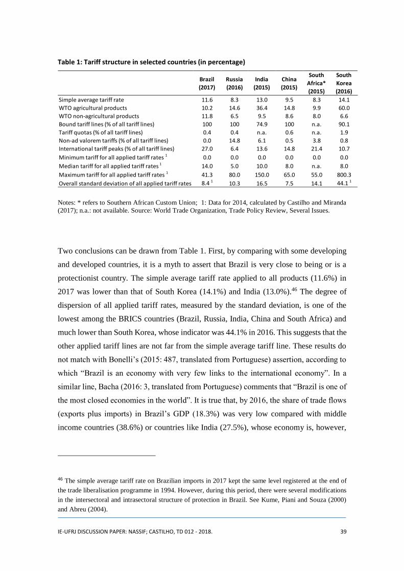
IE-UFRJ DISCUSSION PAPER: NASSIF; CASTILHO, TD 012 - 2018. 39
Table 1: Tariff structure in selected countries (in percentage)
Notes: * refers to Southern African Custom Union; 1: Data for 2014, calculated by Castilho and Miranda
(2017); n.a.: not available. Source: World Trade Organization, Trade Policy Review, Several Issues.
Two conclusions can be drawn from Table 1. First, by comparing with some developing
and developed countries, it is a myth to assert that Brazil is very close to being or is a
protectionist country. The simple average tariff rate applied to all products (11.6%) in
2017 was lower than that of South Korea (14.1%) and India (13.0%).46 The degree of
dispersion of all applied tariff rates, measured by the standard deviation, is one of the
lowest among the BRICS countries (Brazil, Russia, India, China and South Africa) and
much lower than South Korea, whose indicator was 44.1% in 2016. This suggests that the
other applied tariff lines are not far from the simple average tariff line. These results do
not match with Bonelli’s (2015: 487, translated from Portuguese) assertion, according to
which “Brazil is an economy with very few links to the international economy”. In a
similar line, Bacha (2016: 3, translated from Portuguese) comments that “Brazil is one of
the most closed economies in the world”. It is true that, by 2016, the share of trade flows
(exports plus imports) in Brazil’s GDP (18.3%) was very low compared with middle
income countries (38.6%) or countries like India (27.5%), whose economy is, however,
46 The simple average tariff rate on Brazilian imports in 2017 kept the same level registered at the end of
the trade liberalisation programme in 1994. However, during this period, there were several modifications
in the intersectoral and intrasectoral structure of protection in Brazil. See Kume, Piani and Souza (2000)
and Abreu (2004).
Brazil
(2017)
Russia
(2016)
India
(2015)
China
(2015)
South
Africa*
(2015)
South
Korea
(2016)
Simple average tariff rate 11.6 8.3 13.0 9.5 8.3 14.1
WTO agricultural products 10.2 14.6 36.4 14.8 9.9 60.0
WTO non-agricultural products 11.8 6.5 9.5 8.6 8.0 6.6
Bound tariff lines (% of all tariff lines) 100 100 74.9 100 n.a. 90.1
Tariff quotas (% of all tariff lines) 0.4 0.4 n.a. 0.6 n.a. 1.9
Non-ad valorem tariffs (% of all tariff lines) 0.0 14.8 6.1 0.5 3.8 0.8
International tariff peaks (% of all tariff lines) 27.0 6.4 13.6 14.8 21.4 10.7
Minimum tariff for all applied tariff rates 1 0.0 0.0 0.0 0.0 0.0 0.0
Median tariff for all applied tariff rates 1 14.0 5.0 10.0 8.0 n.a. 8.0
Maximum tariff for all applied tariff rates 1 41.3 80.0 150.0 65.0 55.0 800.3
Overall standard deviation of all applied tariff rates 8.4 1 10.3 16.5 7.5 14.1 44.1 1

IE-UFRJ DISCUSSION PAPER: NASSIF; CASTILHO, TD 012 - 2018. 40
more protected than Brazil, as Table 1 shows. However, Brazil’s low degree of trade
openness can be explained by the lack of competitiveness of manufacturing exports as
well as the very low annual GDP growth rates (which imply low import volumes)
observed in the last decades (only 2.4% between 1999 and 2016).47
Second, although the use of the international peaks covers a significant part of all tariff
lines,48 such peaks are in line with the Most Favourable Nation (MFN) tariffs negotiated
multilaterally at the WTO. In any event, Brazilian effective tariff rates estimated by
Castilho and Miranda (2017) for 2014 (an average rate of 16.7% and a standard deviation
of 15.2% for the overall economy) suggest that the structure of protection in Brazil should
be reconsidered taking into account some distortions introduced by the high tariffs of
some industries (e.g. transport equipment and some intermediate goods) as well as by
modifications induced by protectionist lobbies or due to macroeconomic reasons.
From 2003 on, especially during Lula da Silva’s (2003-2010) and Dilma Rousseff’s
governments (2011-2014), industrial policy returned as one of the leading mechanisms
for promoting activities considered strategic for accelerating structural change towards
scale-engineering-and-knowledge-based industries as well as diversifying productive and
export structures, such as capital goods, software, information and communication
technologies, pharmaceutical products, biotechnology, automobiles and others. In this
period, three programmes of industrial policy were announced: Foreign Trade,
Technological and Industrial Policy (PITCE, in Portuguese), in 2004; the Production
Development Policy (PDP), in 2008; and Largest Brazil Plan (Plano Brasil Maior, in
47 The problem of the lack of competitiveness of exports will be discussed in the next subsection. Indicators
on share of trade flows in GDP were drawn from the World Bank, World Economic Indicators.
https://data.worldbank.org/indicator/TG.VAL.TOTL.GD.ZS. Accessed on 13 October 2017. Indicators
on Brazil’s annual GDP growth rates were drawn from the Brazilian Institute of Geography and Trade
(IBGE), Quarterly National Accounts at 1995 constant prices.
https://sidra.ibge.gov.br/pesquisa/cnt/tabelas. Accessed on 13 October 2017.
48 Moreover, for the WTO, tariff peaks correspond to rates exceeding 15%. Other possible definitions take
into account the tariff level and structure of the country. For instance, Castilho and Carvalho (2017)
consider tariff peaks as the rates that exceed the sum of the tariff average and the standard deviation.

IE-UFRJ DISCUSSION PAPER: NASSIF; CASTILHO, TD 012 - 2018. 41
Portuguese – PBM), in 2011.49 All these plans had as their core goal to boost physical
investment and innovation in the Brazilian economy.
These plans, however, repeated old mistakes and well-known misleading policies that
had prevailed during the time of the import substitution period: lack of selectivity and
performance requirements from entrepreneurs who benefited from public incentives; an
excessive use of public subsidies as the main instrument of governmental support,
especially credit subsidies from the Brazilian Development Bank (BNDES); and, last but
not least, lack of coordination between industrial, trade and macroeconomic policies. One
example of coordination failure is related to the recurrent trend of overvaluation of the
Brazilian real. Figure 4 plots the behaviour of the real effective exchange rate (REER) in
Brazil since 1988.50
49 For an analysis of PITCE and PDP industrial policies, see Coutinho et al. (2012). For details on Plano
Brasil Maior, see the website of Brazil’s Ministry of Development, Industry and Commerce (MDIC),
http://www.mdic.gov.br/index.php/competitividade-industrial/politica-industrial/o-que-e-pbm-2 .
Accessed on 12 October 2017.
50 In Brazil, the exchange rate is defined as the domestic price of a foreign currency. So, while an increase
in the exchange rate means a depreciation of the Brazilian real, a decrease means an appreciation of it. The
real effective exchange rate was calculated by the Central Bank as a weighted average of the Brazilian real
against a basket of currencies of Brazil’s main trade partners, adjusted by the consumer inflation rate
(IPCA).
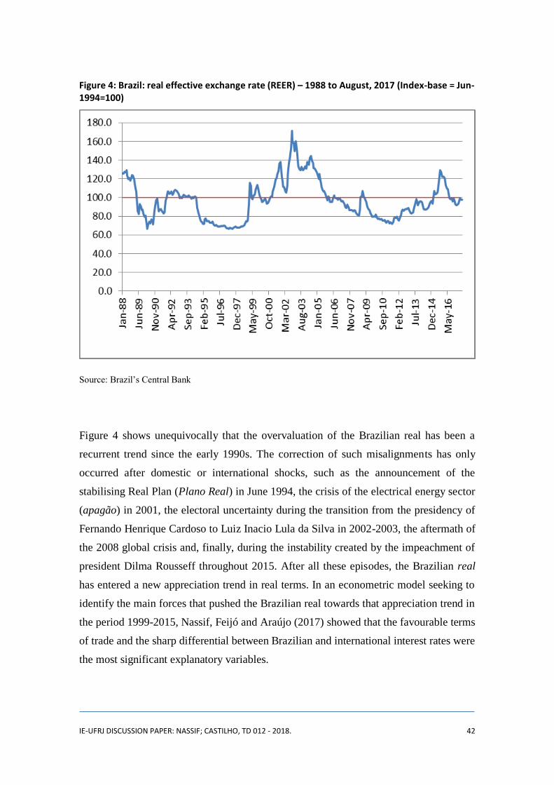
IE-UFRJ DISCUSSION PAPER: NASSIF; CASTILHO, TD 012 - 2018. 42
Figure 4: Brazil: real effective exchange rate (REER) – 1988 to August, 2017 (Index-base = Jun-1994=100)
Source: Brazil’s Central Bank
Figure 4 shows unequivocally that the overvaluation of the Brazilian real has been a
recurrent trend since the early 1990s. The correction of such misalignments has only
occurred after domestic or international shocks, such as the announcement of the
stabilising Real Plan (Plano Real) in June 1994, the crisis of the electrical energy sector
(apagão) in 2001, the electoral uncertainty during the transition from the presidency of
Fernando Henrique Cardoso to Luiz Inacio Lula da Silva in 2002-2003, the aftermath of
the 2008 global crisis and, finally, during the instability created by the impeachment of
president Dilma Rousseff throughout 2015. After all these episodes, the Brazilian real
has entered a new appreciation trend in real terms. In an econometric model seeking to
identify the main forces that pushed the Brazilian real towards that appreciation trend in
the period 1999-2015, Nassif, Feijó and Araújo (2017) showed that the favourable terms
of trade and the sharp differential between Brazilian and international interest rates were
the most significant explanatory variables.
IE-UFRJ DISCUSSION PAPER: NASSIF; CASTILHO, TD 012 - 2018. 43
Several studies have shown a strong correlation between the trend of overvaluation of the
Brazilian real and the weak long-term economic performance of the Brazilian economy,
expressed by a sharp premature deindustrialisation51 as well as low rates of productivity
and economic growth. After having been positively impacted by trade liberalisation
between 1988 and 1998, as previously discussed, the annual average growth rate of labour
productivity in the Brazilian manufacturing sector has been stagnant and showed negative
results between 1999 and 2015 (-0.2% p.y.).52 With such a stagnant performance, it
is not surprising to verify, according to Figure 5, that the technological gap of the
manufacturing sector in Brazil (measured as the ratio of Brazil’s labour productivity to
the U.S. labour productivity), after having shown a slow catching up trajectory between
1970 and 1980, has tendentially widened outwards, as can be seen by the trend line.53
Figure 5 also shows that the last period during which all segments of the Brazilian
manufacturing sector significantly reduced the technological gap occurred in the
aftermath of trade liberalisation, especially between 1990 and 1998, as we discussed
earlier. Particularly, the science-engineering-and-knowledge-based industries, after
having reached almost half of the technological frontier in 1997, entered a falling behind
trajectory afterwards. Although these indicators have not been updated by ECLAC-PADI,
such trends can hardly have registered significant changes in the opposite direction, in the
51 Several studies have attributed the real appreciation trend of the Brazilian currency as being one of the
main causes of Brazil’s premature deindustrialisation. See, for instance, Bacha (2013), Bresser-Pereira
(2010), Nassif, Feijó and Araújo (2015) and Nassif, Bresser-Pereira and Feijó (2017).
52 These results were calculated and kindly offered to the authors by Jorge N.P. Britto, from the Department
of Economics at the Fluminense Federal University. The labour productivity was calculated as the ratio of
the value of industrial transformation (a proxy for value added) to the number of employees directly
occupied at production (these indicators are estimated, in turn, by the Annual Industrial Survey – PIA, from
the Brazilian Institute of Geography and Statistics - IBGE). The numerator was deflated by sectoral
Wholesale Price Indices (IPA) of Fundação Getúlio Vargas.
53 These data are estimated by the Program for the Analysis of Industrial Dynamics (PADI) of the United
Nations Economic Commission for Latin America and the Caribbean (ECLAC). Originally, the taxonomy
of ECLAC is composed by natural resource-based, labour intensive and engineering-based manufacturing
industries. As these latter industries also contain scale and science-based industries, we grouped all of them
and renamed them as science-engineering-and-knowledge-based manufacturing industries.

IE-UFRJ DISCUSSION PAPER: NASSIF; CASTILHO, TD 012 - 2018. 44
face of the stagnant behaviour of the labour productivity growth in the manufacturing
sector in Brazil in the last decade, as we commented earlier.
Figure 5: Technological gap in the Brazilian industries of the manufacturing sector classified by factor content and technological sophistication
Source: ECLAC-PADI
The falling behind trajectory of the Brazilian economy can also be confirmed by the
results of Thirlwall’s law for the Brazilian economy between 1980 and 2010—see
equation (22) in Section 2—, estimated by one of the authors in a previous paper (see
Nassif, Feijó and Araújo, 2015), and summarised in Table 2.
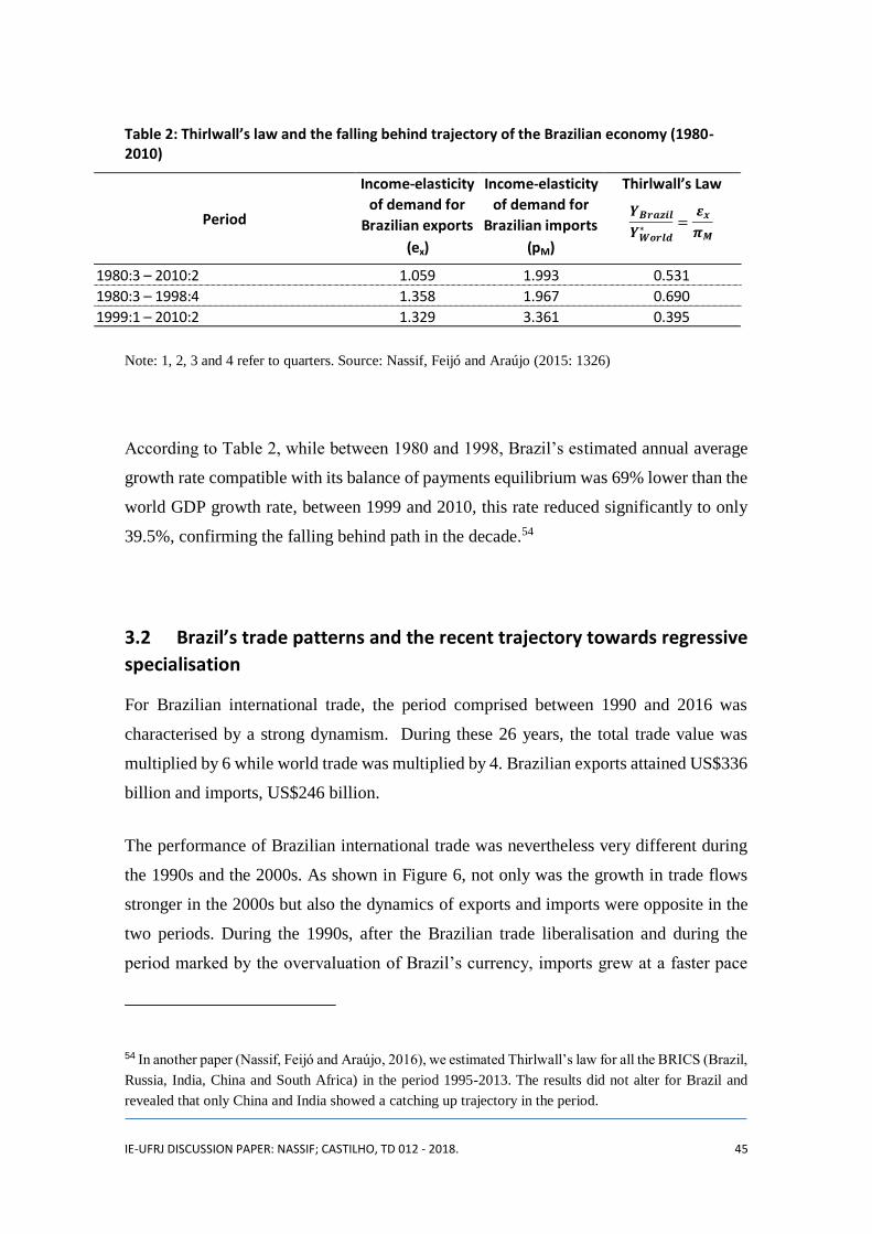
IE-UFRJ DISCUSSION PAPER: NASSIF; CASTILHO, TD 012 - 2018. 45
Table 2: Thirlwall’s law and the falling behind trajectory of the Brazilian economy (1980-2010)
Note: 1, 2, 3 and 4 refer to quarters. Source: Nassif, Feijó and Araújo (2015: 1326)
According to Table 2, while between 1980 and 1998, Brazil’s estimated annual average
growth rate compatible with its balance of payments equilibrium was 69% lower than the
world GDP growth rate, between 1999 and 2010, this rate reduced significantly to only
39.5%, confirming the falling behind path in the decade.54
3.2 Brazil’s trade patterns and the recent trajectory towards regressive
specialisation
For Brazilian international trade, the period comprised between 1990 and 2016 was
characterised by a strong dynamism. During these 26 years, the total trade value was
multiplied by 6 while world trade was multiplied by 4. Brazilian exports attained US$336
billion and imports, US$246 billion.
The performance of Brazilian international trade was nevertheless very different during
the 1990s and the 2000s. As shown in Figure 6, not only was the growth in trade flows
stronger in the 2000s but also the dynamics of exports and imports were opposite in the
two periods. During the 1990s, after the Brazilian trade liberalisation and during the
period marked by the overvaluation of Brazil’s currency, imports grew at a faster pace
54 In another paper (Nassif, Feijó and Araújo, 2016), we estimated Thirlwall’s law for all the BRICS (Brazil,
Russia, India, China and South Africa) in the period 1995-2013. The results did not alter for Brazil and
revealed that only China and India showed a catching up trajectory in the period.
Period
Income-elasticity
of demand for
Brazilian exports
(ex)
Income-elasticity
of demand for
Brazilian imports
(pM)
Thirlwall’s Law
1980:3 – 2010:2 1.059 1.993 0.531
1980:3 – 1998:4 1.358 1.967 0.690
1999:1 – 2010:2 1.329 3.361 0.395
∗ =
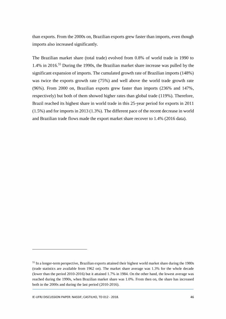
IE-UFRJ DISCUSSION PAPER: NASSIF; CASTILHO, TD 012 - 2018. 46
than exports. From the 2000s on, Brazilian exports grew faster than imports, even though
imports also increased significantly.
The Brazilian market share (total trade) evolved from 0.8% of world trade in 1990 to
1.4% in 2016.55 During the 1990s, the Brazilian market share increase was pulled by the
significant expansion of imports. The cumulated growth rate of Brazilian imports (148%)
was twice the exports growth rate (75%) and well above the world trade growth rate
(96%). From 2000 on, Brazilian exports grew faster than imports (236% and 147%,
respectively) but both of them showed higher rates than global trade (119%). Therefore,
Brazil reached its highest share in world trade in this 25-year period for exports in 2011
(1.5%) and for imports in 2013 (1.3%). The different pace of the recent decrease in world
and Brazilian trade flows made the export market share recover to 1.4% (2016 data).
55 In a longer-term perspective, Brazilian exports attained their highest world market share during the 1980s
(trade statistics are available from 1962 on). The market share average was 1.3% for the whole decade
(lower than the period 2010-2016) but it attained 1.7% in 1984. On the other hand, the lowest average was
reached during the 1990s, when Brazilian market share was 1.0%. From then on, the share has increased
both in the 2000s and during the last period (2010-2016).
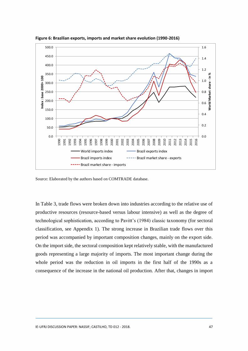
IE-UFRJ DISCUSSION PAPER: NASSIF; CASTILHO, TD 012 - 2018. 47
Figure 6: Brazilian exports, imports and market share evolution (1990-2016)
Source: Elaborated by the authors based on COMTRADE database.
In Table 3, trade flows were broken down into industries according to the relative use of
productive resources (resource-based versus labour intensive) as well as the degree of
technological sophistication, according to Pavitt’s (1984) classic taxonomy (for sectoral
classification, see Appendix 1). The strong increase in Brazilian trade flows over this
period was accompanied by important composition changes, mainly on the export side.
On the import side, the sectoral composition kept relatively stable, with the manufactured
goods representing a large majority of imports. The most important change during the
whole period was the reduction in oil imports in the first half of the 1990s as a
consequence of the increase in the national oil production. After that, changes in import
0.0
0.2
0.4
0.6
0.8
1.0
1.2
1.4
1.6
0.0
50.0
100.0
150.0
200.0
250.0
300.0
350.0
400.0
450.0
500.0
19
90
19
91
19
92
19
93
19
94
19
95
19
96
19
97
19
98
19
99
20
00
20
01
20
02
20
03
20
04
20
05
20
06
20
07
20
08
20
09
20
10
20
11
20
12
20
13
20
14
20
15
20
16
Wo
rld
Mar
ket
shar
e -
in %
Ind
ex
: bas
e 2
00
0=
10
0
World imports index Brazil exports index
Brazil imports index Brazil market share - exports
Brazil market share - imports

IE-UFRJ DISCUSSION PAPER: NASSIF; CASTILHO, TD 012 - 2018. 48
structure were minor, despite the increase in imports of labour and scale intensive
sectors.56
On the export side, as stated, there were important composition changes. The share of
manufactured goods in exports remarkably decreased, going from 78% of total exports in
1990-1995 to 53% in 2011-2016, while the share of primary goods in total exports
increased from 21% to 45% in the same period. In fact, between 1990 and 2016 the share
of primary goods more than doubled and recovered the importance they used to have in
exports in the beginning of the 1970s. This process has been named “export
primarisation” and, as mentioned in section 3.1, several factors explain it, such as the
commodities price boom in the 2000s due to the so-called Chinese demand-pull effect,
the persistent overvaluation of the national currency and the dynamism of domestic
demand for manufactured goods.57 The primarisation process observed in exports was
not, however, observed—at least not with the same intensity—in domestic production. In
fact, Torracca (2017) shows the mismatch between the structure of exports and of
domestic production. While primarisation is clear and strong in external trade flows, the
domestic production structure is much more stable and less intensive in primary goods
and resource based sectors, even though their share in domestic production increased.
These conclusions do not contradict the evidence of premature deindustrialisation in
Brazil, especially from the mid-2000s on. In fact, it is widely recognized that there has
been a sharp reallocation of resources from the manufacturing sector to segments of low
productivity in the tertiary sector in Brazil since the mid-2000s.58
56 The increase in labour intensive imports was strongly influenced by the rise in textiles, clothing, shoes
and some chemical goods, while the transport equipment imports (cars, trucks and ships) were the main
reason for the share of scale intensive goods to increase.
57 See Bacha and Fishlow (2011), Bacha (2013) and Nassif, Feijó and Araújo (2017).
58 In fact, according to the Brazilian Institute of Geography and Statistics (IBGE), the share of the
agricultural sector in Brazil’s GDP in real terms (1995 price) in 2016 was virtually the same as that of 1996
(6%). Yet, while the share of the manufacturing sector in total GDP was reduced from 13.8% to 9.8%, the
share of the tertiary sector was increased from 57% to 60.7% during the same period. See
https://www.ibge.gov.br/estatisticas-novoportal/economicas/contas-nacionais/9300-contas-nacionais-
trimestrais.html?&t=resultados. Accessed on 25 October 2017. See Nassif (2008) for the 1947-2004 period
(in current prices).
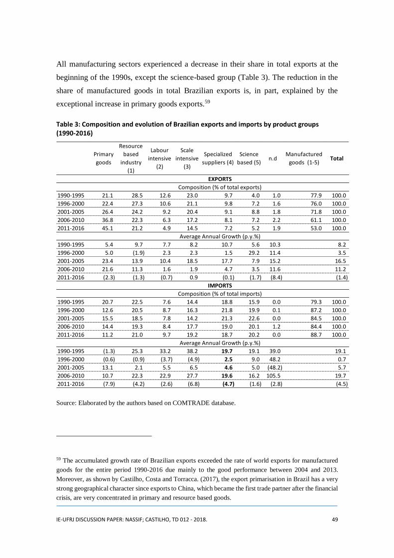
IE-UFRJ DISCUSSION PAPER: NASSIF; CASTILHO, TD 012 - 2018. 49
All manufacturing sectors experienced a decrease in their share in total exports at the
beginning of the 1990s, except the science-based group (Table 3). The reduction in the
share of manufactured goods in total Brazilian exports is, in part, explained by the
exceptional increase in primary goods exports.59
Table 3: Composition and evolution of Brazilian exports and imports by product groups (1990-2016)
Source: Elaborated by the authors based on COMTRADE database.
59 The accumulated growth rate of Brazilian exports exceeded the rate of world exports for manufactured
goods for the entire period 1990-2016 due mainly to the good performance between 2004 and 2013.
Moreover, as shown by Castilho, Costa and Torracca. (2017), the export primarisation in Brazil has a very
strong geographical character since exports to China, which became the first trade partner after the financial
crisis, are very concentrated in primary and resource based goods.
Primary
goods
Resource
based
industry
(1)
Labour
intensive
(2)
Scale
intensive
(3)
Specialized
suppliers (4)
Science
based (5)n.d
Manufactured
goods (1-5)Total
1990-1995 21.1 28.5 12.6 23.0 9.7 4.0 1.0 77.9 100.0
1996-2000 22.4 27.3 10.6 21.1 9.8 7.2 1.6 76.0 100.0
2001-2005 26.4 24.2 9.2 20.4 9.1 8.8 1.8 71.8 100.0
2006-2010 36.8 22.3 6.3 17.2 8.1 7.2 2.2 61.1 100.0
2011-2016 45.1 21.2 4.9 14.5 7.2 5.2 1.9 53.0 100.0
1990-1995 5.4 9.7 7.7 8.2 10.7 5.6 10.3 8.2
1996-2000 5.0 (1.9) 2.3 2.3 1.5 29.2 11.4 3.5
2001-2005 23.4 13.9 10.4 18.5 17.7 7.9 15.2 16.5
2006-2010 21.6 11.3 1.6 1.9 4.7 3.5 11.6 11.2
2011-2016 (2.3) (1.3) (0.7) 0.9 (0.1) (1.7) (8.4) (1.4)
1990-1995 20.7 22.5 7.6 14.4 18.8 15.9 0.0 79.3 100.0
1996-2000 12.6 20.5 8.7 16.3 21.8 19.9 0.1 87.2 100.0
2001-2005 15.5 18.5 7.8 14.2 21.3 22.6 0.0 84.5 100.0
2006-2010 14.4 19.3 8.4 17.7 19.0 20.1 1.2 84.4 100.0
2011-2016 11.2 21.0 9.7 19.2 18.7 20.2 0.0 88.7 100.0
1990-1995 (1.3) 25.3 33.2 38.2 19.7 19.1 39.0 19.1
1996-2000 (0.6) (0.9) (3.7) (4.9) 2.5 9.0 48.2 0.7
2001-2005 13.1 2.1 5.5 6.5 4.6 5.0 (48.2) 5.7
2006-2010 10.7 22.3 22.9 27.7 19.6 16.2 105.5 19.7
2011-2016 (7.9) (4.2) (2.6) (6.8) (4.7) (1.6) (2.8) (4.5)
Average Annual Growth (p.y.%)
EXPORTS
Composition (% of total exports)
Average Annual Growth (p.y.%)
IMPORTS
Composition (% of total imports)
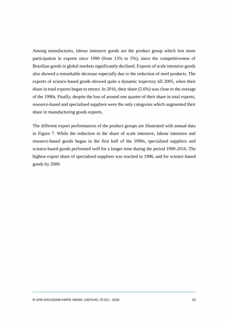
IE-UFRJ DISCUSSION PAPER: NASSIF; CASTILHO, TD 012 - 2018. 50
Among manufactures, labour intensive goods are the product group which lost more
participation in exports since 1990 (from 13% to 5%), since the competitiveness of
Brazilian goods in global markets significantly declined. Exports of scale intensive goods
also showed a remarkable decrease especially due to the reduction of steel products. The
exports of science-based goods showed quite a dynamic trajectory till 2005, when their
share in total exports began to retract. In 2016, their share (5.6%) was close to the average
of the 1990s. Finally, despite the loss of around one quarter of their share in total exports,
resource-based and specialised suppliers were the only categories which augmented their
share in manufacturing goods exports.
The different export performances of the product groups are illustrated with annual data
in Figure 7. While the reduction in the share of scale intensive, labour intensive and
resource-based goods began in the first half of the 1990s, specialised suppliers and
science-based goods performed well for a longer time during the period 1990-2016. The
highest export share of specialised suppliers was reached in 1996, and for science-based
goods by 2000.
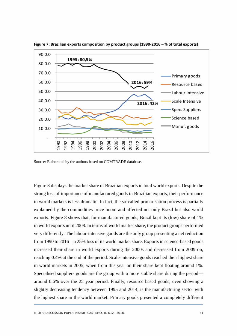
IE-UFRJ DISCUSSION PAPER: NASSIF; CASTILHO, TD 012 - 2018. 51
Figure 7: Brazilian exports composition by product groups (1990-2016 – % of total exports)
Source: Elaborated by the authors based on COMTRADE database.
Figure 8 displays the market share of Brazilian exports in total world exports. Despite the
strong loss of importance of manufactured goods in Brazilian exports, their performance
in world markets is less dramatic. In fact, the so-called primarisation process is partially
explained by the commodities price boom and affected not only Brazil but also world
exports. Figure 8 shows that, for manufactured goods, Brazil kept its (low) share of 1%
in world exports until 2008. In terms of world market share, the product groups performed
very differently. The labour-intensive goods are the only group presenting a net reduction
from 1990 to 2016—a 25% loss of its world market share. Exports in science-based goods
increased their share in world exports during the 2000s and decreased from 2009 on,
reaching 0.4% at the end of the period. Scale-intensive goods reached their highest share
in world markets in 2005, when from this year on their share kept floating around 1%.
Specialised suppliers goods are the group with a more stable share during the period—
around 0.6% over the 25 year period. Finally, resource-based goods, even showing a
slightly decreasing tendency between 1995 and 2014, is the manufacturing sector with
the highest share in the world market. Primary goods presented a completely different
2016: 42%
1995: 80,5%
2016: 59%
-
10.0.0
20.0.0
30.0.0
40.0.0
50.0.0
60.0.0
70.0.0
80.0.0
90.0.01
990
19
92
19
94
19
96
19
98
20
00
20
02
20
04
20
06
20
08
20
10
20
12
20
14
20
16
Primary goods
Resource based
Labour intensive
Scale Intensive
Spec. Suppliers
Science based
Manuf. goods

IE-UFRJ DISCUSSION PAPER: NASSIF; CASTILHO, TD 012 - 2018. 52
performance: their market share, after a decade of relative stability of around 1.8% in the
1990s, was multiplied by 3.4 by 2016. Brazilian primary goods exports represented in
that year 6.3% of total world exports.
Figure 8: Market share of Brazilian exports in world exports, by product group, (1990-2016, % of world exports)
Source: Elaborated by the authors based on COMTRADE database.
A traditional indicator of a country’s pattern of specialisation is Balassa’s (1965)
Revealed Comparative Advantage (RCA) [see equation A.1 in Appendix 2], whose
results are shown in Figure 9.60 Indicators clearly register a deepening of Brazilian export
specialisation based on primary goods. Since it was accompanied by a continuous drop
of the RCA of several manufactured goods categories (notably, labour-intensive, science-
60 If RCA is above 1, that means the country has comparative advantage, whereas if RCA is below 1, that
means absence of comparative advantage—or comparative disadvantage.
3.8
1.9
1.0
1.3
0.70.7
1.5
1.00.9
0.00
0.50
1.00
1.50
2.00
2.50
3.00
3.50
4.00
Primary goods
Resource based
Labour intensive
Scale Intensive
Spec. Suppliers
Science based
Total
Manufactured goods
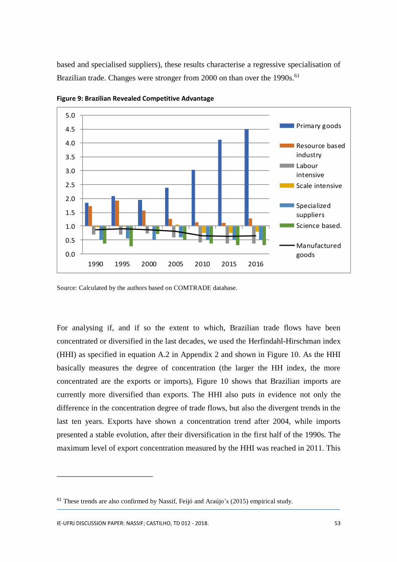
IE-UFRJ DISCUSSION PAPER: NASSIF; CASTILHO, TD 012 - 2018. 53
based and specialised suppliers), these results characterise a regressive specialisation of
Brazilian trade. Changes were stronger from 2000 on than over the 1990s.61
Figure 9: Brazilian Revealed Competitive Advantage
Source: Calculated by the authors based on COMTRADE database.
For analysing if, and if so the extent to which, Brazilian trade flows have been
concentrated or diversified in the last decades, we used the Herfindahl-Hirschman index
(HHI) as specified in equation A.2 in Appendix 2 and shown in Figure 10. As the HHI
basically measures the degree of concentration (the larger the HH index, the more
concentrated are the exports or imports), Figure 10 shows that Brazilian imports are
currently more diversified than exports. The HHI also puts in evidence not only the
difference in the concentration degree of trade flows, but also the divergent trends in the
last ten years. Exports have shown a concentration trend after 2004, while imports
presented a stable evolution, after their diversification in the first half of the 1990s. The
maximum level of export concentration measured by the HHI was reached in 2011. This
61 These trends are also confirmed by Nassif, Feijó and Araújo’s (2015) empirical study.
0.0
0.5
1.0
1.5
2.0
2.5
3.0
3.5
4.0
4.5
5.0
1990 1995 2000 2005 2010 2015 2016
Primary goods
Resource based
industry
Labour
intensive
Scale intensive
Specialized
suppliers
Science based.
Manufactured
goods

IE-UFRJ DISCUSSION PAPER: NASSIF; CASTILHO, TD 012 - 2018. 54
latter result reflects the emergence of China as one of the most important Brazilian trade
partners after the 2008 global crisis. In fact, Brazilian exports grew sharply and became
extremely concentrated in mineral ores, soybeans and oil.62
Figure 10: Degree of concentration of Brazilian exports and imports (Herfindahl-Hirschman Index, 1990-2016)
Source: Calculated by the authors based on COMTRADE database.
Table 4 shows the HHI for exports classified by factor content and technological
sophistication. The major concentration changes occurred with the science-based goods,
-which showed the highest degree of export concentration by 2016. This was due to the
high share of aircraft exports in this group. 63 The above mentioned “China effect” has
clearly influenced the high concentration of primary and resource-based goods. The
62 These three products represent around 75% of Brazilian exports to China. As international prices of these
commodities were very high until 2012, the share of these products in total exports rose remarkably.
63 Since 1990, airplanes have been the most important product in the science-based category. In the first
half of the 1990s, they accounted for a quarter of this category’s exports and reached 46% in 2016.
0,000
0,010
0,020
0,030
0,040
0,050
0,060
1990
1991
1992
1993
1994
1995
1996
1997
1998
1999
2000
2001
2002
2003
2004
2005
2006
2007
2008
2009
2010
2011
2012
2013
2014
2015
2016
Exports Imports

IE-UFRJ DISCUSSION PAPER: NASSIF; CASTILHO, TD 012 - 2018. 55
group of scale-intensive goods is the one that exhibited the most stable degree of export
concentration in the whole period.
Table 4: Concentration of Brazilian exports, by product group (HH Index, 1990-2016)
Source: Calculated by the authors, based on COMTRADE database.
Another way of evaluating the degree of diversification is to measure the extent to which
Brazil has exported old and established goods in the world markets (intensive margin) or
new products and other goods with increasing share in world exports (extensive margin).
The intensive (IM) and extensive (EM) margins were calculated according to the
methodology proposed by Hummels and Klenow (2005) and are expressed by equations
A.3 and A.4, presented in Appendix 2.64 The former corresponds to a country’s market
share of world exports in the products or categories in which it exports, indicating how
consolidated the country is in exporting the same category of goods in the markets it
traditionally acts in. The latter corresponds to the share of a country’s export basket in
world exports through the diversification of exports in new categories of goods. The EM
also aims at showing how important the country’s export basket (or its ‘portfolio’) is for
the world market.65
64 There are other different definitions such as the one used by Amurgo-Pacheco and Pierola (2008) which
identifies “old” and “new” import and export products and markets of a country by comparing the existence
of trade flows with a reference period.
65 According to Hummels and Klenow (2005), export growth can result from the expansion of exports of
goods already exported or from a diversification process which corresponds to the “enlargement of the
1990 1995 2000 2005 2010 2016
Primary goods 0.186 0.181 0.156 0.149 0.181 0.149
Resource based industry 0.094 0.077 0.068 0.072 0.122 0.117
Labour intensive 0.126 0.107 0.110 0.097 0.099 0.116
Scale intensive 0.093 0.086 0.089 0.086 0.086 0.084
Specialized suppliers 0.129 0.079 0.087 0.089 0.081 0.086
Science based 0.190 0.090 0.331 0.223 0.192 0.250
TOTAL 0.025 0.021 0.022 0.023 0.044 0.035
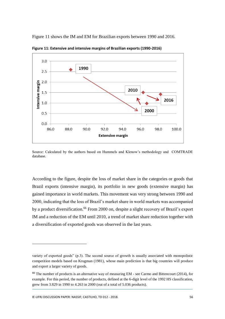
IE-UFRJ DISCUSSION PAPER: NASSIF; CASTILHO, TD 012 - 2018. 56
Figure 11 shows the IM and EM for Brazilian exports between 1990 and 2016.
Figure 11: Extensive and intensive margins of Brazilian exports (1990-2016)
Source: Calculated by the authors based on Hummels and Klenow’s methodology and COMTRADE
database.
According to the figure, despite the loss of market share in the categories or goods that
Brazil exports (intensive margin), its portfolio in new goods (extensive margin) has
gained importance in world markets. This movement was very strong between 1990 and
2000, indicating that the loss of Brazil’s market share in world markets was accompanied
by a product diversification.66 From 2000 on, despite a slight recovery of Brazil’s export
IM and a reduction of the EM until 2010, a trend of market share reduction together with
a diversification of exported goods was observed in the last years.
variety of exported goods” (p.3). The second source of growth is usually associated with monopolistic
competition models based on Krugman (1981), whose main prediction is that big countries will produce
and export a larger variety of goods.
66 The number of products is an alternative way of measuring EM - see Carmo and Bittencourt (2014), for
example. For this period, the number of products, defined at the 6-digit level of the 1992 HS classification,
grew from 3.829 in 1990 to 4.263 in 2000 (out of a total of 5.036 products).
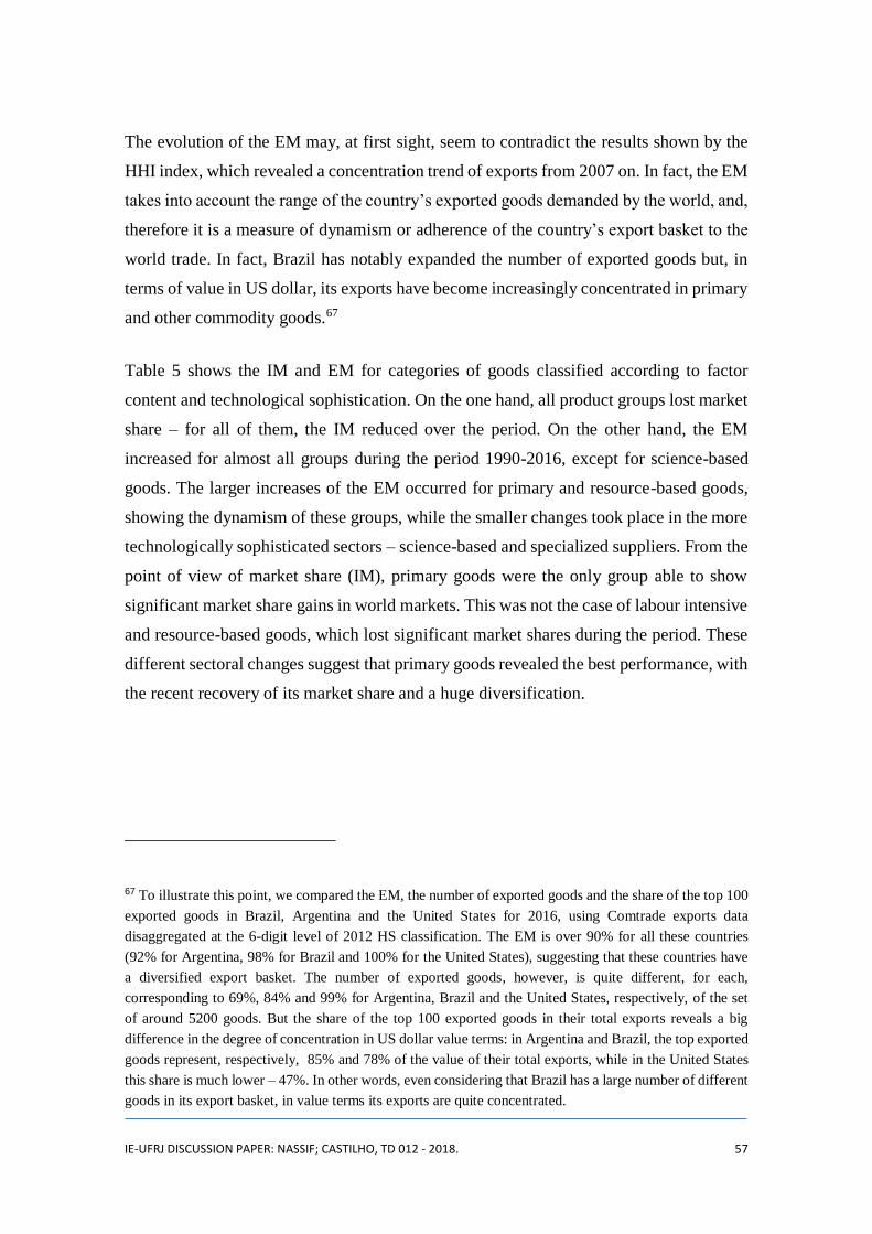
IE-UFRJ DISCUSSION PAPER: NASSIF; CASTILHO, TD 012 - 2018. 57
The evolution of the EM may, at first sight, seem to contradict the results shown by the
HHI index, which revealed a concentration trend of exports from 2007 on. In fact, the EM
takes into account the range of the country’s exported goods demanded by the world, and,
therefore it is a measure of dynamism or adherence of the country’s export basket to the
world trade. In fact, Brazil has notably expanded the number of exported goods but, in
terms of value in US dollar, its exports have become increasingly concentrated in primary
and other commodity goods.67
Table 5 shows the IM and EM for categories of goods classified according to factor
content and technological sophistication. On the one hand, all product groups lost market
share – for all of them, the IM reduced over the period. On the other hand, the EM
increased for almost all groups during the period 1990-2016, except for science-based
goods. The larger increases of the EM occurred for primary and resource-based goods,
showing the dynamism of these groups, while the smaller changes took place in the more
technologically sophisticated sectors – science-based and specialized suppliers. From the
point of view of market share (IM), primary goods were the only group able to show
significant market share gains in world markets. This was not the case of labour intensive
and resource-based goods, which lost significant market shares during the period. These
different sectoral changes suggest that primary goods revealed the best performance, with
the recent recovery of its market share and a huge diversification.
67 To illustrate this point, we compared the EM, the number of exported goods and the share of the top 100
exported goods in Brazil, Argentina and the United States for 2016, using Comtrade exports data
disaggregated at the 6-digit level of 2012 HS classification. The EM is over 90% for all these countries
(92% for Argentina, 98% for Brazil and 100% for the United States), suggesting that these countries have
a diversified export basket. The number of exported goods, however, is quite different, for each,
corresponding to 69%, 84% and 99% for Argentina, Brazil and the United States, respectively, of the set
of around 5200 goods. But the share of the top 100 exported goods in their total exports reveals a big
difference in the degree of concentration in US dollar value terms: in Argentina and Brazil, the top exported
goods represent, respectively, 85% and 78% of the value of their total exports, while in the United States
this share is much lower – 47%. In other words, even considering that Brazil has a large number of different
goods in its export basket, in value terms its exports are quite concentrated.
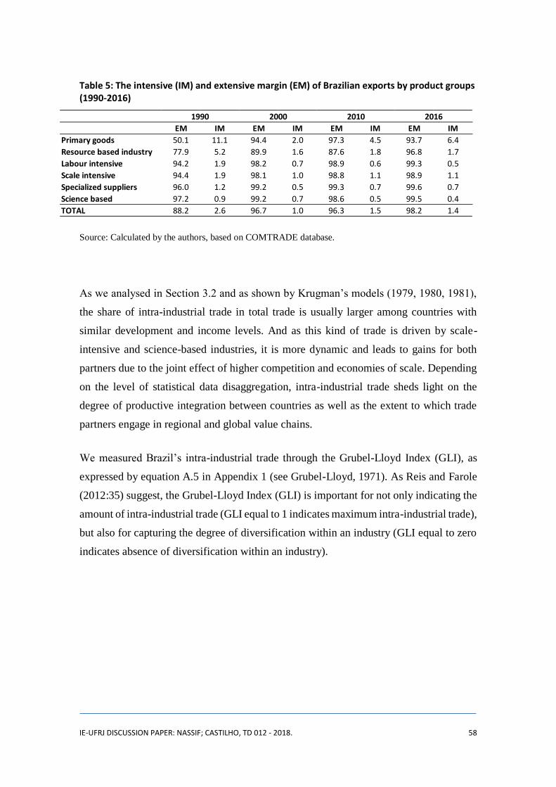
IE-UFRJ DISCUSSION PAPER: NASSIF; CASTILHO, TD 012 - 2018. 58
Table 5: The intensive (IM) and extensive margin (EM) of Brazilian exports by product groups (1990-2016)
Source: Calculated by the authors, based on COMTRADE database.
As we analysed in Section 3.2 and as shown by Krugman’s models (1979, 1980, 1981),
the share of intra-industrial trade in total trade is usually larger among countries with
similar development and income levels. And as this kind of trade is driven by scale-
intensive and science-based industries, it is more dynamic and leads to gains for both
partners due to the joint effect of higher competition and economies of scale. Depending
on the level of statistical data disaggregation, intra-industrial trade sheds light on the
degree of productive integration between countries as well as the extent to which trade
partners engage in regional and global value chains.
We measured Brazil’s intra-industrial trade through the Grubel-Lloyd Index (GLI), as
expressed by equation A.5 in Appendix 1 (see Grubel-Lloyd, 1971). As Reis and Farole
(2012:35) suggest, the Grubel-Lloyd Index (GLI) is important for not only indicating the
amount of intra-industrial trade (GLI equal to 1 indicates maximum intra-industrial trade),
but also for capturing the degree of diversification within an industry (GLI equal to zero
indicates absence of diversification within an industry).
EM IM EM IM EM IM EM IM
Primary goods 50.1 11.1 94.4 2.0 97.3 4.5 93.7 6.4
Resource based industry 77.9 5.2 89.9 1.6 87.6 1.8 96.8 1.7
Labour intensive 94.2 1.9 98.2 0.7 98.9 0.6 99.3 0.5
Scale intensive 94.4 1.9 98.1 1.0 98.8 1.1 98.9 1.1
Specialized suppliers 96.0 1.2 99.2 0.5 99.3 0.7 99.6 0.7
Science based 97.2 0.9 99.2 0.7 98.6 0.5 99.5 0.4
TOTAL 88.2 2.6 96.7 1.0 96.3 1.5 98.2 1.4
1990 2000 2010 2016
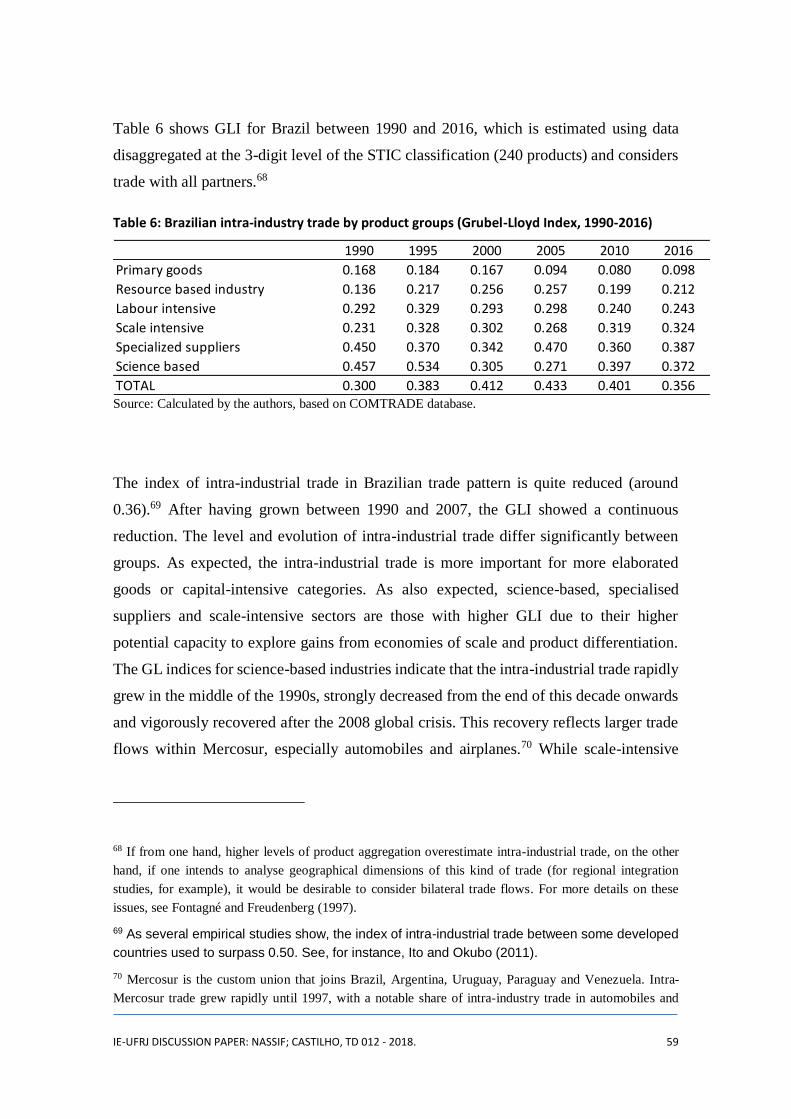
IE-UFRJ DISCUSSION PAPER: NASSIF; CASTILHO, TD 012 - 2018. 59
Table 6 shows GLI for Brazil between 1990 and 2016, which is estimated using data
disaggregated at the 3-digit level of the STIC classification (240 products) and considers
trade with all partners.68
Table 6: Brazilian intra-industry trade by product groups (Grubel-Lloyd Index, 1990-2016)
Source: Calculated by the authors, based on COMTRADE database.
The index of intra-industrial trade in Brazilian trade pattern is quite reduced (around
0.36).69 After having grown between 1990 and 2007, the GLI showed a continuous
reduction. The level and evolution of intra-industrial trade differ significantly between
groups. As expected, the intra-industrial trade is more important for more elaborated
goods or capital-intensive categories. As also expected, science-based, specialised
suppliers and scale-intensive sectors are those with higher GLI due to their higher
potential capacity to explore gains from economies of scale and product differentiation.
The GL indices for science-based industries indicate that the intra-industrial trade rapidly
grew in the middle of the 1990s, strongly decreased from the end of this decade onwards
and vigorously recovered after the 2008 global crisis. This recovery reflects larger trade
flows within Mercosur, especially automobiles and airplanes.70 While scale-intensive
68 If from one hand, higher levels of product aggregation overestimate intra-industrial trade, on the other
hand, if one intends to analyse geographical dimensions of this kind of trade (for regional integration
studies, for example), it would be desirable to consider bilateral trade flows. For more details on these
issues, see Fontagné and Freudenberg (1997).
69 As several empirical studies show, the index of intra-industrial trade between some developed
countries used to surpass 0.50. See, for instance, Ito and Okubo (2011).
70 Mercosur is the custom union that joins Brazil, Argentina, Uruguay, Paraguay and Venezuela. Intra-
Mercosur trade grew rapidly until 1997, with a notable share of intra-industry trade in automobiles and
1990 1995 2000 2005 2010 2016
Primary goods 0.168 0.184 0.167 0.094 0.080 0.098
Resource based industry 0.136 0.217 0.256 0.257 0.199 0.212
Labour intensive 0.292 0.329 0.293 0.298 0.240 0.243
Scale intensive 0.231 0.328 0.302 0.268 0.319 0.324
Specialized suppliers 0.450 0.370 0.342 0.470 0.360 0.387
Science based 0.457 0.534 0.305 0.271 0.397 0.372
TOTAL 0.300 0.383 0.412 0.433 0.401 0.356

IE-UFRJ DISCUSSION PAPER: NASSIF; CASTILHO, TD 012 - 2018. 60
industries increased their GLI between 1990 and 2016, specialised suppliers and labour-
intensive showed reductions. As expected, the primary goods and the resource-based
groups show the smallest values for the GLI in the period.
Table 7 shows the composition of exports and imports according to Brazil’s trade partners
(1990 – 2016). Table 7 suggests that Brazil can be classified as a “global trader” because
of its large variety of trade partners. Over the period 1990-2016, there were some
important changes in the geographical composition of Brazilian trade. First, its most
traditional partners (the United States and the European Union (EU))71 lost importance
throughout this period. This reduction is stronger on the export side of Brazil, while on
the import side, the EU kept its share in the Brazilian market. Brazil’s export share in
Latin American countries increased during the 1990s, when they became a major
destination for Brazilian exports. Mercosur was the main market responsible for this
change, which is also confirmed by the huge rise of Argentinean share both in exports
and imports. After 2000, bilateral trade with Argentina declined, affecting Latin
America’s total trade. Even after this decline, Latin America remained as one of Brazil’s
most important partners, especially on the export side. Another marked change in
Brazilian trade was the increase of China’s share in Brazilian trade after 2010. While in
2000, China’s share for Brazilian exports and imports was around 2% of Brazil’s total
trade, this indicator jumped after the 2008 global crisis, reaching 19.2% and 17%,
respectively, in 2016.
capital goods sectors. The intra-regional trade was so negatively affected by the 1998-1999 Brazilian crisis
and the 1999-2001 Argentinean crisis that it was not returned to the 1990s level.
71 Here we kept the 12 countries belonging to the EU in 1990 and that remained the main partners (more
than 90% of EU27 trade).

IE-UFRJ DISCUSSION PAPER: NASSIF; CASTILHO, TD 012 - 2018. 61
Table 7: Geographical distribution of Brazilian exports and imports
(1990-2016; in percentage)
Notes: n.a.: not available. Elaborated by the authors based on COMTRADE database.
Despite the fact that Brazil’s trade with other countries (South Korea, Japan, Russia and
India, as described in Table 8) is not as expressive as that with China and the United
States, the data suggests that there was a geographical deconcentration of Brazilian
exports and, albeit to a lesser extent, of imports. In fact, during the 2000s, trade with Asia
and Africa grew and diversified, even taking into account that trade with these two regions
(except China) remained relatively weak.
The changes in geographical composition of Brazilian exports are reflected in the sectoral
specialisation of the Brazilian export basket. In fact, Brazil’s trade structure differs
according to the stage of development of its trade partners and the specialisation of the
partners. Bilateral trade can have a kind of North-South pattern of specialisation, as
analysed in sections 2.2.1 and 2.3. That is, Brazil’s trade pattern with the European Union
and China is different from that with Mercosur or other neighbouring countries. As shown
by Castilho, Costa and Torracca (2017), in the last decade, the Brazilian export structure
was strongly influenced by trade with China, which is very concentrated in mineral and
agricultural goods. In a simple simulation, they show that the share of manufactured
EXPORT IMPORT EXPORT IMPORT EXPORT IMPORT EXPORT IMPORT
Latin America 11.0 12.5 24.8 21.7 21.6 15.3 19.5 12.1
Argentina 2.1 6.7 11.5 12.3 9.3 8.0 7.3 6.6
Mexico 1.6 0.9 3.2 1.4 1.9 2.1 2.1 2.6
United States 24.6 20.1 24.7 23.4 9.8 15.1 12.7 17.5
European Union 12 28.3 19.4 26.5 22.9 20.4 18.5 16.8 19.4
China 1.2 0.9 2.0 2.2 15.5 14.1 19.2 17.0
India 0.5 0.1 0.4 0.5 1.8 2.3 1.7 1.8
Japan 7.5 7.2 4.6 5.3 3.6 3.9 2.5 2.6
South Korea 1.7 0.4 1.1 2.6 1.9 4.7 1.6 4.0
Russia n.a. n.a. 0.8 1.0 2.1 1.1 1.3 1.5
World 100.0 100.0 100.0 100.0 100.0 100.0 100.0 100.0
1990 2000 2010 2016
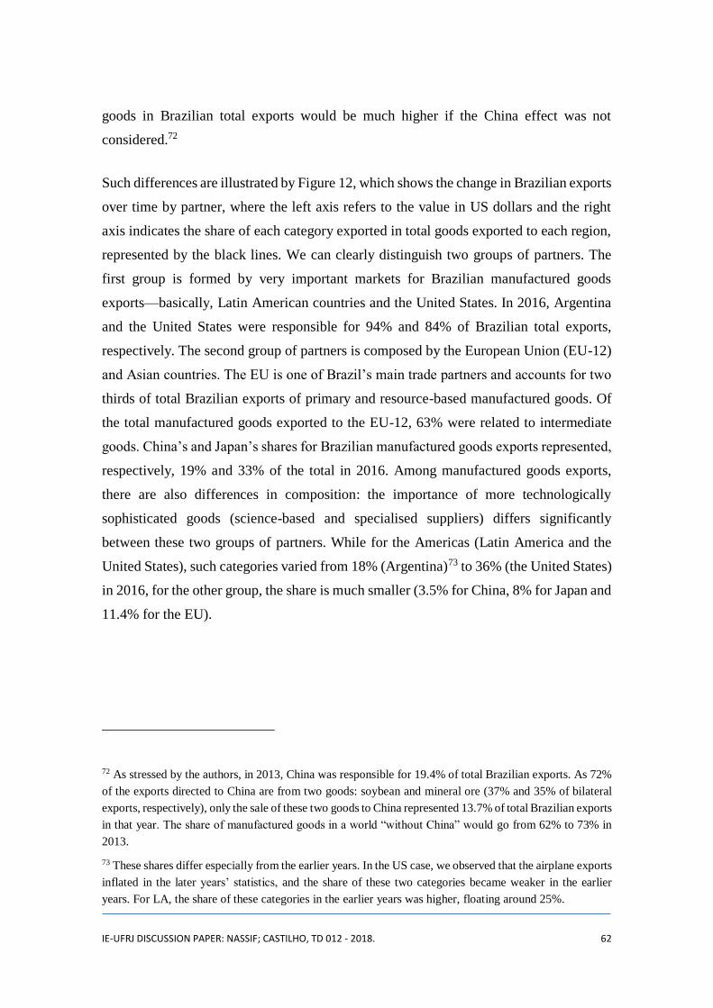
IE-UFRJ DISCUSSION PAPER: NASSIF; CASTILHO, TD 012 - 2018. 62
goods in Brazilian total exports would be much higher if the China effect was not
considered.72
Such differences are illustrated by Figure 12, which shows the change in Brazilian exports
over time by partner, where the left axis refers to the value in US dollars and the right
axis indicates the share of each category exported in total goods exported to each region,
represented by the black lines. We can clearly distinguish two groups of partners. The
first group is formed by very important markets for Brazilian manufactured goods
exports—basically, Latin American countries and the United States. In 2016, Argentina
and the United States were responsible for 94% and 84% of Brazilian total exports,
respectively. The second group of partners is composed by the European Union (EU-12)
and Asian countries. The EU is one of Brazil’s main trade partners and accounts for two
thirds of total Brazilian exports of primary and resource-based manufactured goods. Of
the total manufactured goods exported to the EU-12, 63% were related to intermediate
goods. China’s and Japan’s shares for Brazilian manufactured goods exports represented,
respectively, 19% and 33% of the total in 2016. Among manufactured goods exports,
there are also differences in composition: the importance of more technologically
sophisticated goods (science-based and specialised suppliers) differs significantly
between these two groups of partners. While for the Americas (Latin America and the
United States), such categories varied from 18% (Argentina)73 to 36% (the United States)
in 2016, for the other group, the share is much smaller (3.5% for China, 8% for Japan and
11.4% for the EU).
72 As stressed by the authors, in 2013, China was responsible for 19.4% of total Brazilian exports. As 72%
of the exports directed to China are from two goods: soybean and mineral ore (37% and 35% of bilateral
exports, respectively), only the sale of these two goods to China represented 13.7% of total Brazilian exports
in that year. The share of manufactured goods in a world “without China” would go from 62% to 73% in
2013.
73 These shares differ especially from the earlier years. In the US case, we observed that the airplane exports
inflated in the later years’ statistics, and the share of these two categories became weaker in the earlier
years. For LA, the share of these categories in the earlier years was higher, floating around 25%.
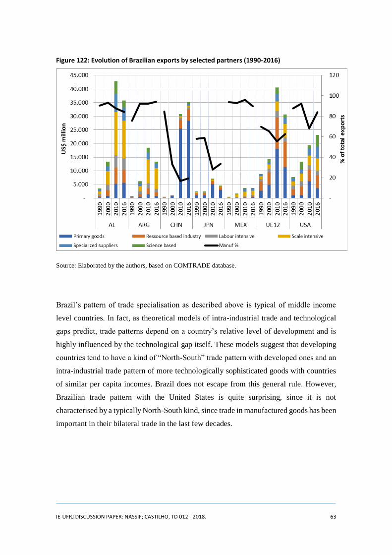
IE-UFRJ DISCUSSION PAPER: NASSIF; CASTILHO, TD 012 - 2018. 63
Figure 122: Evolution of Brazilian exports by selected partners (1990-2016)
Source: Elaborated by the authors, based on COMTRADE database.
Brazil’s pattern of trade specialisation as described above is typical of middle income
level countries. In fact, as theoretical models of intra-industrial trade and technological
gaps predict, trade patterns depend on a country’s relative level of development and is
highly influenced by the technological gap itself. These models suggest that developing
countries tend to have a kind of “North-South” trade pattern with developed ones and an
intra-industrial trade pattern of more technologically sophisticated goods with countries
of similar per capita incomes. Brazil does not escape from this general rule. However,
Brazilian trade pattern with the United States is quite surprising, since it is not
characterised by a typically North-South kind, since trade in manufactured goods has been
important in their bilateral trade in the last few decades.
IE-UFRJ DISCUSSION PAPER: NASSIF; CASTILHO, TD 012 - 2018. 64
4 Concluding remarks
This paper analysed the performance and composition of Brazilian trade flows in the last
26 years. Since most conventional theoretical models reviewed in this study, including
the so-called “new new trade” models, take either technology or factor endowments as
exogenous, they are insufficient to capture some essential elements of developing
countries’ pattern of specialisation. In particular, as these countries are characterised by
large technological and productivity gaps compared with developed countries, descriptive
statistics indicators are insufficient to evaluate the extent to which unconditional
engagement in free trade policies can positively or negatively affect their long-term
growth. The main contribution of Structuralist-Neoschumpeterian models is to show that
the extent of a country’s technological gap affects its pattern of specialisation and growth
dynamics. Specifically, they predict that a country characterised by regressive trade
specialisation has low export diversification as well as income-elasticity of demand for
its exports lower than income-elasticity of demand for its imports, implying a perverse
long-term growth dynamics and compromising a virtuous catching up trajectory.
Empirical evidence on Brazil showed that since the early-2000s the technological gaps of
the manufacturing sector (including natural resource-based segments) have significantly
increased. In addition, as the income-elasticity of demand for Brazilian exports has
become expressively smaller than the income-elasticity of demand for Brazilian imports
after 1999, in comparison with the period 1980-1998, Brazil’s estimated long-term
growth rate compatible with its balance of payments equilibrium has been much lower
than the world growth rate. According to Thirlwall’s Law (1979), such performance
marks a falling-behind path.
The analysis of Brazilian trade pattern evidenced its regressive trade specialisation.
Despite the significant increase of Brazilian trade flows, the country’s trade pattern did
not show a virtuous trajectory between 1990 and 2016, especially with respect to the
observed changes in the export structure. While the import structure remained relatively
stable, with the more technologically sophisticated sectors accounting for around 40% of
Brazilian imports since the mid-1990s, the export structure was marked by a severe
primarisation process. The export of primary goods continued to increase its share in
Brazil until 2014, even after the reversal of the commodity price boom from 2011
IE-UFRJ DISCUSSION PAPER: NASSIF; CASTILHO, TD 012 - 2018. 65
onwards. Among manufactured goods exports, labour-intensive and technologically
sophisticated ones, such as scale and specialised suppliers, were replaced by primary and
resource-based ones. The share of all resource-based segments (primary and resource-
based manufactured goods) more than doubled over the last 26 years, reaching 60% of
Brazilian total exports in 2016.
This primarisation phenomenon was reinforced by a concentration trend of Brazilian
exports. Although Brazil’s ability to export new goods and diversify them for new
markets (the extensive margin) increased for almost all categories of goods (except for
science-based ones) between 1990 and 2016, these results did not imply a true
diversification trend. Indeed, despite Brazil having notably expanded the number of
exported goods, its exported value in US dollars, however, became highly concentrated
in commodity goods in the same period. As to the geographical composition of trade
flows, although Brazil can be considered a global trader because its trade relations are
relatively diversified in the global economy, its bilateral trade patterns differ considerably
according to the trade partners in terms of composition, diversification and degree of
sophistication. While Brazil’s bilateral trade with China, which became the most
important Brazilian trade partner after the 2008 global crisis, is characterised by a typical
“North-South” trade pattern, the Brazilian trade pattern with Latin American countries is
radically different. By being characterised by sectoral complementarities and intra-
industrial trade, this suggests a major potential for generating dynamic gains from trade
between Brazil and Latin America.
Since Brazil had a sharp regressive trade specialisation in the last decades, such a trend
has normative implications that go beyond the scope of this study. Notwithstanding, it is
worth noting that appropriate industrial and trade policies finely coordinated with other
economic policies (including the macroeconomic ones) are necessary for boosting
productivity as well as changing this current regressive trade pattern into another
characterised by diversification of Brazilian exports towards technologically
sophisticated manufactured goods. This strategy could help put Brazil in a successful
catching up trajectory.
IE-UFRJ DISCUSSION PAPER: NASSIF; CASTILHO, TD 012 - 2018. 66
References
ABRAMOVITZ, M. Catching up, forging ahead and falling behind”. Journal of
Economic History, n. 46, p. 385-406, 1986.
ABREU, M.P. Trade Liberalization and the Political Economy of Protection in Brazil
since 1987. Working Paper-SITI-08B. Buenos Aires, Institute for the Integration of Latin
America and the Caribbean – IDB-INTAL.
AMSDEM, A. H. (2001), The Rise of “the Rest”: Challenges to the West from Late-
Industrializing Economies. Oxford, Oxford University Press.
AMURGO-PACHECO, A.; PIEROLA, M. (2008). “Patterns of Export Diversification in
Developing Countries: Intensive and Extensive Margins”. Policy Research Working
Paper; No. 4473. World Bank, Washington, DC.
BACHA, E. (2016). “Integrar para Crescer 2.0”. Texto para Discussão no. 36. Rio de
Janeiro: IEPE-Casa das Garças.
BACHA, E. and FISHLOW, A. (2011). The Recent Commodity Price Boom and Latin
American Growth: More than New Bottles for an Old Wine? In José A. Ocampo and
Jaime Ros (ed.). The Oxford Handbook of Latin American Economics. Oxford: Oxford
University Press,
BACHA, E. L. (2013). “Bonança externa e desindustrialização: uma análise do período
2005-2011” In: E. Bacha and M. B. de Bolle (orgs). O Futuro da Indústria no Brasil:
desindustrialização em debate”. Rio de Janeiro: Civilização Brasileira, 2013.
BALASSA, B. (1965). “Trade Liberalisation and Revealed Comparative Advantage”.
The Manchester School, Volume 33, Issue 2, May, Pages 99–123.
BHAGWATI, J. (1978). Anatomy and Consequences of Exchange Control Regimes.
Cambridge (Mas.): Ballinger Pub. Company.

IE-UFRJ DISCUSSION PAPER: NASSIF; CASTILHO, TD 012 - 2018. 67
BONELLI, R. (2002). Labor Productivity in Brazil during the 1990’s. Texto para
Discussão no 906. Rio de Janeiro: IPEA.
BONELLI, R. (2015). “Comparações Internacionais de Produtividade na Indústria e
Tendências Setoriais: Brasil e EUA”. In: BARBOSA, N. et al. (org.). Indústria e
Desenvolvimento Produtivo no Brasil. Rio de Janeiro: Fundação Getúlio Vargas: 487-
517.
BONELLI, R. e FONSECA, R. (1998). “Ganhos de Produtividade e de Eficiência: Novos
Resultados para a Economia Brasileira”. Texto para Discussão nº 557. Rio de Janeiro:
IPEA.
BRESSER-PEREIRA, L.C.(2010). Globalization and competition. Why some emerging
countries succeed while others fall behind. Cambridge: Cambridge University Press.
CARVALHO JR., M. C. (1992). “Alguns Aspectos da Reforma Aduaneira Recente”.
Texto para Discussão no 74. Rio de Janeiro: FUNCEX, novembro.
CASTILHO, M. and MIRANDA, P. (2017) Tarifa aduaneira como instrumento de
política industrial: a evolução da estrutura de proteção tarifária no Brasil no período 2004-
2014 e sua comparação com outros países. IPEA, mimeo.
CASTILHO, M., COSTA, K. and TORRACA, J. (2017). A Importância do Mercado
Latino-Americano e da Competição Chinesa para o Desempenho Recente das
Exportações Brasileiras de Produtos Manufaturados, Revista de Análise Econômica,
forthcoming.
CARMO, A. and BITTENCOURT, M. (2014) O Efeito da Volatilidade da Taxa de
Câmbio sobre o Comércio Internacional: Uma Investigação Empírica sob a Ótica da
Margem Extensiva. Estudos Econômicos, vol.44, n.4, p.815-845.
CIMOLI, M. (1988). “Technological Gaps and Institutional Asymmetries in a North-
South Model with a Continuum of Goods”. Metroeconomica 39: 245-274.
IE-UFRJ DISCUSSION PAPER: NASSIF; CASTILHO, TD 012 - 2018. 68
CIMOLI, M. and PORCILE, G. (2010). “Specialization, Wage Bargaining and
Technology in a Multigoods Growth Model”. Metroeconomica 61:1: 219-238.
CIMOLI, M. and SOETE, L. (1988). “A Generalised Technological Gap Trade Model”.
Paper presented at the Conference on Technological Innovations and Organization.
Triestre, September.
CIMOLI, M., DOSI, G. and SOETE, L. (1986). “Innovation Diffusion, Institutional
Differences and Patterns of Trade: a North-South Model. Brighton, SPRU, University of
Sussex. Paper originally presented at the Conference on Innovation Diffusion, Venice,
17-21 March 1986.
COUTINHO, L. (1997). “A Especialização Regressiva: um Balanço do Desempenho
Industrial pós-estabilização. In: J. P. R. Velloso (coord.). Brasil: Desafios de um País em
Transformação. Rio de Janeiro: José Olympio.
COUTINHO, L., FERRAZ, J.C., NASSIF, A. and OLIVA, R. (2012). “Industrial Policy
and Economic Transformation” In: Santiso, J. and J. Dayton-Johnson. Oxford: Oxford
University Press.
DALHMAN C.J. and FRISCHTAK C.R. (1993). National Systems supporting Technical
Advance in Industry: the Brazilian Experience. In: Nelson RR, ed. National Innovation
Systems: A Comparative Analysis. Oxford University Press, New York and Oxford.
DORNBUSCH, R. FISCHER, S. and SAMUELSON, P. (1977). “Comparative
Advantage, Trade and Payments in a Ricardian Model with a Continuum of Goods”. The
American Economic Review 67: 823-839. December.
DOSI, G. and SOETE, G. (1988). “Technical Change and International Trade”. In: G.
Dosi, C. Freeman, R. Nelson, .R G. Silverberg and L. Soete (eds). Technical Change and
Economic Theory. London: Pinter-Publishers: 401-431.
DOSI, G., PAVITT, K. e SOETE, L. (1990). The Economics of Technical Change and
International Trade. London: Harvester Wheastsheaf.
IE-UFRJ DISCUSSION PAPER: NASSIF; CASTILHO, TD 012 - 2018. 69
EATON, J. and KORTUM, S. (2002). “Technology, Geography, and Trade: Firms,
Industries, and Export Destination". Econometrica 70: 1741-1779.
FEENSTRA, R.C.. (2004). Advanced International Trade: Theory and Evidence.
Princeton: Princeton University Press.
FEIJÓ, C. A. and CARVALHO, P. G. M. (1994). Sete Teses Equivocadas sobre o
aumento da Produtividade Industrial nos anos Recentes. Boletim de Conjuntura. Rio de
Janeiro: IE/UFRJ.
FINGER, J. and KREININ, M. (1979) A measure of ‘export similarity’ and its possible
uses. The economic journal, v. 89, nº. 36: 905-912.
FONTAGNÉ, L. and FREUDENBERG, M. (1997) Intra-Industry Trade: Methodological
Issues Reconsidered, Working Papers 1997-01, CEPII Research Center.
FURTADO, C. (1959). Formação Econômica do Brasil. 18a. ed. Cia Editora Nacional,
1982.
GERSCHENKRON, A. (1962). Economic backwardness in historical perspective.
Cambridge (Ma.): Harvard University Press, 1962.
GROSSMAN, G. M. and HELPMAN, E. (1991). Innovation and Growth in the Global
Economy. Cambridge (Mas.): The MIT Press.
GRUBEL, H. and LLOYD, P. (1971) The Empirical Measurement of Intra-Industry
Trade. Economic Record. 47 (4): 494–517.
HAY, D. A. (1997). “The Post 1990 Brazilian Trade Liberalization and the Performance
of Large Manufacturing Firms: Productivity, Market Share and Profits”. Texto para
Discussão n. 523. Rio de Janeiro: IPEA, outubro.
HECKSCHER, E.F. (1919). “The Effect of Foreign Trade on the Distribution of National
Income” In: Flam, H. e J. Flanders (ed.). Heckscher-Ohlin Trade Theory. Cambridge
(Mas): The MIT Press, 1991.
IE-UFRJ DISCUSSION PAPER: NASSIF; CASTILHO, TD 012 - 2018. 70
HELPMAN, E. (1984). “A Simple Theory of International Trade with Multinational
Corporations”. Journal of Political Economy 92: 451-471.
HELPMAN, E. and KRUGMAN, P. R. (1985). Market Structure and Foreign Trade.
Cambridge (Mas): The MIT Press.
GRAHAM, F. D. (1923). “Some Aspects of Protection Further Considered”. Quarterly
Journal of Economics 37: 199-227, February.
HELPMAN, Elhanan (2011). Understanding Global Trade. Cambridge: Harvard
University Press.
HUMMELS, D. and KLENOW, P. (2005) The Variety and Quality of a Nation’s Exports.
American Economic Review, Vol. 95 No. 3: 704-723.
IMBS, J., and WACZIARG, R. 2003. “Stages of Diversification.” American Economic
Review. 93 (1): 63–86.
ITO and OKUBO, (2011). New Aspects of Intra-Industry Trade. Evidence from EU-15
Countries. Discussion Paper Series RIEB DP-2011-02. Kobe University.
KALDOR, N. (1966). Causes of the slow rate of economic growth of the United Kingdom.
An inaugural lecture. Cambridge : Cambridge University Press.
KRUGMAN, P. R. (1990). “Introduction” In: Krugman, P.R. Rethinking International
Trade. Cambridge (Mas.): The MIT Press.
KRUGMAN, P. R. (1979). "Increasing Returns, Monopolistic Competition, and
International Trade”. Journal of International Economics, 9 (4): 469-479. November.
KRUGMAN, P. R. (1980). “Scale Economies, Product Differentiation, and the Pattern of
Trade. American Economic Review 70: 950-959.
KRUGMAN, P. R. (1981). “Intraindustry Specialization and the Gains from Trade”.
Journal of Political Economy, 89 (5): 959-974.

IE-UFRJ DISCUSSION PAPER: NASSIF; CASTILHO, TD 012 - 2018. 71
KRUGMAN, P. R. (1990). “Increasing Returns and the Theory of International Trade”.
In: P.R. Krugman. Rethinking International Trade. Cambridge, Mas.: Cambridge
University Press.
KUME, H., PIANI, G. and SOUZA, C.F.B. (2000). “A Política Brasileira de Importação
no Período 1987-98: Descrição e Avaliação”. Rio de Janeiro, IPEA, mimeo.
KUPFER, D. (2005). “Tecnologia e Emprego são Realmente Antagônicos?” In: J. Sicsú,
L.F. de Paula e R. Michel. Novo Desenvolvimentismo: Um Projeto Nacional de
Crescimento com Equidade Social. São Paulo: Ed. Manole.
LEONTIEF, W. (1953). “Domestic Production and Foreign Trade: the American Capital
Position Re-examined”. Proceedings of the American Philosophical Society 97:332-349.
LINDER, Staffan B. (1961). An Essay on Trade and Transformation. New York: Wiley.
HELPMAN, Elhanam e KRUGMAN, Paul R. (1985). Market Structure and Foreign
Trade. Cambridge (Mas): The MIT Press.
MARKUSEN, J.R. (1984). “Multinationals Firms and the Theory of International
Trade”. Cambridge, Ma.: MIT Press.
MARKUSEN, J.R. (1984). “Multinationals, Multi-Plant Economies and the Gains from
Trade”. Journal of International Economics 16: 205-216.
MCDOUGALL, G.D.A. (1951). “British and American Exports: A Study Suggested by
the Theory of Comparative Costs”. Economic Journal 61, December: 697-724.
MCKINNON, R. (1991). The Order of Economic Liberalization: Financial Control in
the Transition to a Market Economy. Baltimore: The John Hopkins University Press.
MELITZ, Marc and TREFLER, Daniel (2012). Gains from Trade When Firms Matter.
Journal of Economic Perspectives, Vol. 26, no 2, Spring: 91-118.
MELITZ, Marc J. 2003. “The Impact of Trade on Intra-Industry Reallocations and
Aggregate Industry Productivity.” Econometrica 71(6): 1695–1725.
IE-UFRJ DISCUSSION PAPER: NASSIF; CASTILHO, TD 012 - 2018. 72
MICHAELY, M. M., PAPAGEORGIU, D., e CHOSKI, A. (1991). Liberalizing Foreign
Trade: Lessons of Experience in the Developing World. Vol.7. Cambridge (Mas.): Basil
Blackwell.
MILL, J. S. (1848). Principles of Political Economy. Baltimore: Penguin Books, 1970.
MOREIRA, M. M. and Correa, P.; “A First Look at the Impacts of Trade Liberalization
on Brazilian Manufacturing Industry”. World Development, Vol. 26, No. 10, pp. 1859-
1874, 1998.
MOREIRA, M.M. (1995). Industrialization, Trade and Market Failures: The Role of
Government Intervention in Brazil and South Korea. London:Palgrave MacMillan.
NASSIF, A. (2003). Liberalização Comercial e Eficiência Econômica: a Experiência
Brasileira. PhD Thesis. Rio de Janeiro: IE-Universidade Federal do Rio de Janeiro.
NASSIF, A. (2005). “As Fontes de Mudança da Eficiência Técnica da Indústria Brasileira
após a Liberalização Comercial: uma Estimação Econométrica por Dados de Painéis.
Economia Aplicada no. 9 (1): abril-junho: 301-324.
NASSIF, A. (2007). National Innovation System and Macroeconomic Policies: Brazil
and India in Comparative Perspective. UNCTAD Discussion Papers no. 184. Geneva:
United Nations Conference on Trade and Development.
NASSIF, A. (2008). “Há evidências de desindustrialização no Brasil?”, Revista de
Economia Política, vol. 28, N° 1, São Paulo.
NASSIF, A. L. (1995). "Política Industrial e Proteção no Brasil: o Papel da CACEX".
Dissertação de Mestrado. Niterói: Universidade Federal Fluminense.
NASSIF, A., BRESSER-PEREIRA, L.C. and FEIJÓ, C. (2017). “The Case for
Reindustrialisation in Developing Countries: Towards the Connection Between the
Macroeconomic Regime and the Industrial Policy in Brazil”. Cambridge Journal of
Economics, Advanced on line copy doi:10.1093/cje/bex028: 1-27.

IE-UFRJ DISCUSSION PAPER: NASSIF; CASTILHO, TD 012 - 2018. 73
NASSIF, A., FEIJÓ, C. and ARAÚJO, E. (2016). “Structural Change, Catching Up and
Falling Behind in the BRICS: A Comparative Analysis based on Trade Patterns and
Thirlwall’s Law”. PSL Quarterly Review, vol. 69 no. 278, December: 373-421
NASSIF, A., FEIJÓ, C. and ARAÚJO, E. (2017). “A Structuralist-Keynesian Model for
Determining the “Optimum” Real Exchange Rate for Brazil’s Economic Development
Process: 1999-2015”. CEPAL Review. December, forthcoming.
Nassif, A., Feijó, C., and Araújo, E. (2015). “Structural change and economic
development: is Brazil catching or falling behind?”. Cambridge Journal of Economics,
vol. 39, no. 5: 1307-1332, 2015.
OECD (2012). “Industrial Policy and Territorial Development: Lessons from Korea”.
Development Centre Studies. Paris: Organisation for Economic Co-Operation and
Development (OECD).
OHLIN, B. (1924). A Theory of Trade. Ph.D. Dissertation. Stockholm School of
Economics. In: Flam, H. e J. Flanders (ed.). Heckscher-Ohlin Trade Theory. Cambridge
(Mas.): The MIT Press, 1991.
OHLIN, B. (1933). Interregional and International Trade. Cambridge (Mas.): Harvard
University Press, 1968.
OREIRO, J. L. and FEIJÓ, C. (2010). “Desindustrialização: conceituação, causas, efeitos
e o caso brasileiro”. Revista de Economia Política (Brazilian Journal of Political
Economy). Vol. 30, nº 2 (118):219-232, abril-junho.
PAVITT, K. (1984). Sectoral Patterns of Technical Change: Towards a Taxonomy and a
Theory. Research Policy 13: 343-373.
POSNER, M. (1961). International Trade and Technical Change. Oxford Economic
Papers, Vol. 13.
IE-UFRJ DISCUSSION PAPER: NASSIF; CASTILHO, TD 012 - 2018. 74
PREBISCH, R. (1950). The Economic Development of Latin America and its Principal
Problems. New York: Economic Comission for Latin America, United Nations
Department of Economic Affairs.
REIS, J. G. and FAROLE, T. (2012). Trade Competitiveness Diagnostic Toolkit.
Washington, D.C.: The World Bank.
RICARDO (1817). On the Principles of Political Economy and Taxation. Piero Sraffa’s
Edition. Cambridge: Cambridge University Press, 1951.
ROSSI Jr., J. L. e FERREIRA, P. C. (1999). “Evolução da Produtividade Industrial
Brasileira e Abertura Comercial”. Texto para Discussão no. 651. Rio de Janeiro: IPEA.
RYBCZYNSKI, T. M. (1955). “Factor Endowment and the Relative Commodity Prices”.
Economica 22: 336-341.
SAMUELSON, Paul A. (1948). International Trade and the Equalization of Factor Prices.
Economic Journal , 58: 168-184.
SAMUELSON, P. A. (1949). International Factor Price Equalization once Again”. The
Economic Journal 59:181-197.
SMITH, A. (1776). An Inquiry into the Nature and Causes of the Wealth of Nations. New
York: Modern Library, 1937.
STOLPER, W. and SAMUELSON, P. A. (1941). “Protection and Real Wages”. Review
of Economic Studies 9: 58-73.
TAVARES, M. C. (1963). “Auge e Declínio do Processo de Substituição de Importações
no Brasil”. In: Tavares, M.C. Da Substituição de Importações ao Capitalismo Financeiro.
Ensaios sobre a Economia Brasileira. 10ª ed. Rio de Janeiro: Zahar Editores.
THIRLWALL, A.P. (2011a), “The Balance of Payments Constraint as an Explanation of
the International Growth Rate Differences”. PSL Quarterly Review, vol. 64 n. 259, pp.
429-438.

IE-UFRJ DISCUSSION PAPER: NASSIF; CASTILHO, TD 012 - 2018. 75
TORRACCA, J. (2017) Coevolução das Estruturas de Produção e Comércio Exterior da
Indústria Brasileira: Convergência ou Desarticulação? PhD Thesis. Rio de Janeiro, IE-
Universidade Federal do Rio de Janeiro.
VANEK , J. (1968). "The Factor Proportions Theory: the N-Factor Case". Kyklos. 21:
749-756. October.
VERNON, R. (1966).”International Investment and International Trade in the Product
Cycle”. The Quarterly Journal of Economics, 80: 190-207

IE-UFRJ DISCUSSION PAPER: NASSIF; CASTILHO, TD 012 - 2018. 76
Appendix 1
Classification of Brazilian Industries according to Factor Content and
Technological Sophistication (Correspondence between STIC Revision 2
and Pavitt’s taxonomy)
STIC-Rev 2 Product Description Product Categories (Pavitt
Taxonomy) Pavitt’s Codes
001 Live animals chiefly for food Primary goods 110
011 Meat,edible meat offals, fresh, chi Primary goods 110
012 Meat & edible offals,salted,in brin Primary goods 110
014 Meat & edib.offals,prep./pres.,fish Primary goods 110
025 Eggs and yolks,fresh,dried or other Primary goods 110
034 Fish,fresh (live or dead),chilled o Primary goods 110
041 Wheat (including spelt) and meslin, Primary goods 110
042 Rice Primary goods 110
043 Barley,unmilled Primary goods 110
044 Maize (corn),unmilled Primary goods 110
045 Cereals,unmilled ( no wheat,rice,ba Primary goods 110
054 Vegetab.,fresh,chilled,frozen/pres. Primary goods 110
057 Fruit & nuts(not includ. oil nuts), Primary goods 110
071 Coffee and coffee substitutes Primary goods 110
072 Cocoa Primary goods 110
074 Tea and mate Primary goods 110
075 Spices Primary goods 110
121 Tobacco,unmanufactured; tobacco ref Primary goods 110
211 Hides and skins (except furskins), Primary goods 110
212 Furskins,raw (includ.astrakhan,cara Primary goods 110
222 Oil seeds and oleaginous fruit,whol Primary goods 110
244 Cork,natural,raw & waste (includ.in Primary goods 110
245 Fuel wood (excluding wood waste) an Primary goods 110
246 Pulpwood (including chips and wood Primary goods 110
247 Other wood in the rough or roughly Primary goods 110
261 Silk Primary goods 110
264 Jute & other textile bast fibres,ne Primary goods 110
265 Vegetable textile fibres and waste Primary goods 110
291 Crude animal materials,n.e.s. Primary goods 110
292 Crude vegetable materials, n.e.s. Primary goods 110
273 Stone,sand and gravel Primary goods 120
274 Sulphur and unroasted iron pyrites Primary goods 120
277 Natural abrasives,n.e.s (incl.indus Primary goods 120
278 Other crude minerals Primary goods 120
281 Iron ore and concentrates Primary goods 120
286 Ores and concentrates of uranium an Primary goods 120
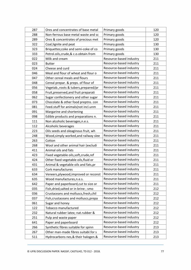
IE-UFRJ DISCUSSION PAPER: NASSIF; CASTILHO, TD 012 - 2018. 77
287 Ores and concentrates of base metal Primary goods 120
288 Non-ferrous base metal waste and sc Primary goods 120
289 Ores & concentrates of precious met Primary goods 120
322 Coal,lignite and peat Primary goods 130
323 Briquettes;coke and semi-coke of co Primary goods 130
333 Petrol.oils,crude,& c.o.obtain.from Primary goods 130
022 Milk and cream Resource-based industry 211
023 Butter Resource-based industry 211
024 Cheese and curd Resource-based industry 211
046 Meal and flour of wheat and flour o Resource-based industry 211
047 Other cereal meals and flours Resource-based industry 211
048 Cereal prepar. & preps. of flour of Resource-based industry 211
056 Vegetab.,roots & tubers,prepared/pr Resource-based industry 211
058 Fruit,preserved,and fruit preparati Resource-based industry 211
062 Sugar confectionery and other sugar Resource-based industry 211
073 Chocolate & other food preptns. con Resource-based industry 211
081 Feed.stuff for animals(not incl.unm Resource-based industry 211
091 Margarine and shortening Resource-based industry 211
098 Edible products and preparations n. Resource-based industry 211
111 Non alcoholic beverages,n.e.s. Resource-based industry 211
112 Alcoholic beverages Resource-based industry 211
223 Oils seeds and oleaginous fruit, wh Resource-based industry 211
248 Wood,simply worked,and railway slee Resource-based industry 211
263 Cotton Resource-based industry 211
268 Wool and other animal hair (excludi Resource-based industry 211
411 Animal oils and fats Resource-based industry 211
423 Fixed vegetable oils,soft,crude,ref Resource-based industry 211
424 Other fixed vegetable oils,fluid or Resource-based industry 211
431 Animal & vegetable oils and fats,pr Resource-based industry 211
633 Cork manufactures Resource-based industry 211
634 Veneers,plywood,improved or reconst Resource-based industry 211
635 Wood manufactures,n.e.s. Resource-based industry 211
642 Paper and paperboard,cut to size or Resource-based industry 211
035 Fish,dried,salted or in brine ; smo Resource-based industry 212
036 Crustaceans and molluscs,fresh,chil Resource-based industry 212
037 Fish,crustaceans and molluscs,prepa Resource-based industry 212
061 Sugar and honey Resource-based industry 212
122 Tobacco manufactured Resource-based industry 212
232 Natural rubber latex; nat.rubber & Resource-based industry 212
251 Pulp and waste paper Resource-based industry 212
641 Paper and paperboard Resource-based industry 212
266 Synthetic fibres suitable for spinn Resource-based industry 213
267 Other man-made fibres suitabl.for s Resource-based industry 213
511 Hydrocarbons nes,& their halogen.& Resource-based industry 213
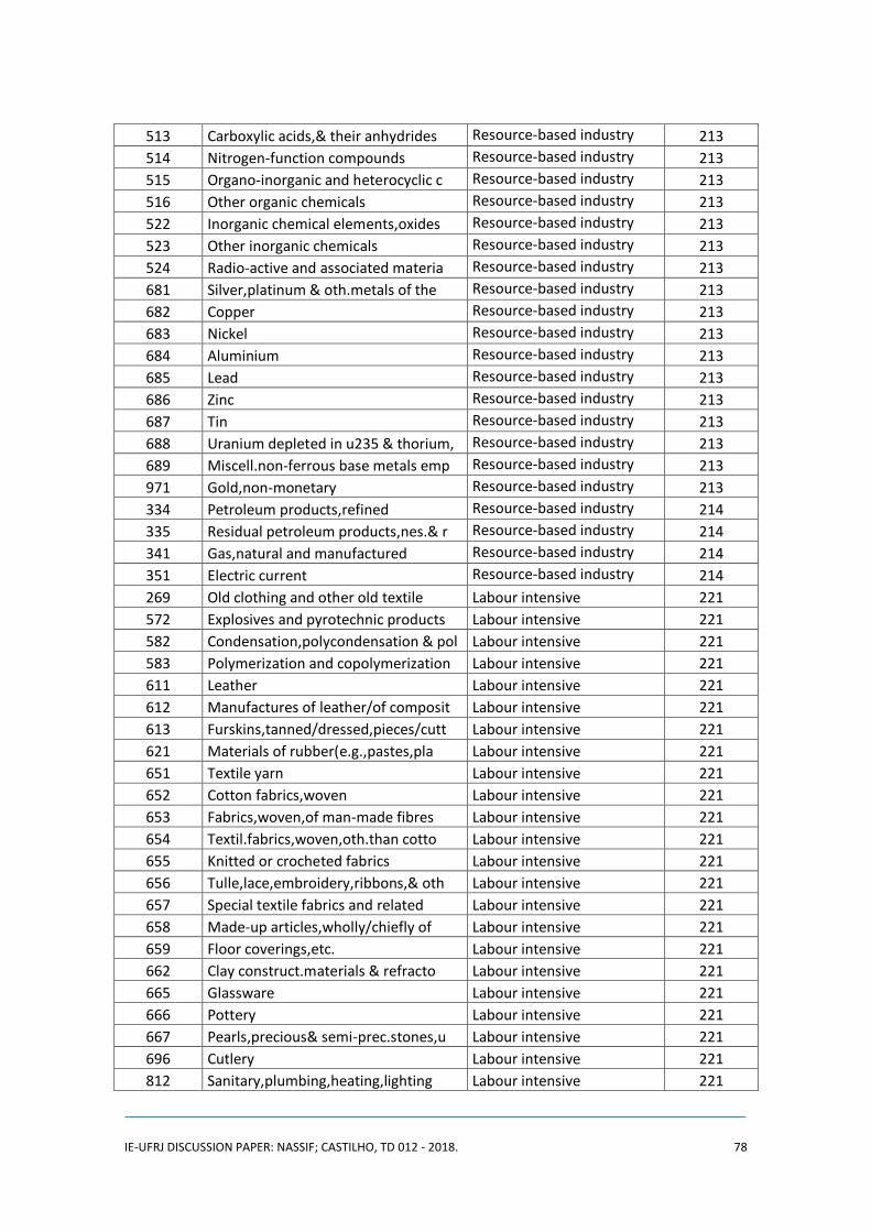
IE-UFRJ DISCUSSION PAPER: NASSIF; CASTILHO, TD 012 - 2018. 78
513 Carboxylic acids,& their anhydrides Resource-based industry 213
514 Nitrogen-function compounds Resource-based industry 213
515 Organo-inorganic and heterocyclic c Resource-based industry 213
516 Other organic chemicals Resource-based industry 213
522 Inorganic chemical elements,oxides Resource-based industry 213
523 Other inorganic chemicals Resource-based industry 213
524 Radio-active and associated materia Resource-based industry 213
681 Silver,platinum & oth.metals of the Resource-based industry 213
682 Copper Resource-based industry 213
683 Nickel Resource-based industry 213
684 Aluminium Resource-based industry 213
685 Lead Resource-based industry 213
686 Zinc Resource-based industry 213
687 Tin Resource-based industry 213
688 Uranium depleted in u235 & thorium, Resource-based industry 213
689 Miscell.non-ferrous base metals emp Resource-based industry 213
971 Gold,non-monetary Resource-based industry 213
334 Petroleum products,refined Resource-based industry 214
335 Residual petroleum products,nes.& r Resource-based industry 214
341 Gas,natural and manufactured Resource-based industry 214
351 Electric current Resource-based industry 214
269 Old clothing and other old textile Labour intensive 221
572 Explosives and pyrotechnic products Labour intensive 221
582 Condensation,polycondensation & pol Labour intensive 221
583 Polymerization and copolymerization Labour intensive 221
611 Leather Labour intensive 221
612 Manufactures of leather/of composit Labour intensive 221
613 Furskins,tanned/dressed,pieces/cutt Labour intensive 221
621 Materials of rubber(e.g.,pastes,pla Labour intensive 221
651 Textile yarn Labour intensive 221
652 Cotton fabrics,woven Labour intensive 221
653 Fabrics,woven,of man-made fibres Labour intensive 221
654 Textil.fabrics,woven,oth.than cotto Labour intensive 221
655 Knitted or crocheted fabrics Labour intensive 221
656 Tulle,lace,embroidery,ribbons,& oth Labour intensive 221
657 Special textile fabrics and related Labour intensive 221
658 Made-up articles,wholly/chiefly of Labour intensive 221
659 Floor coverings,etc. Labour intensive 221
662 Clay construct.materials & refracto Labour intensive 221
665 Glassware Labour intensive 221
666 Pottery Labour intensive 221
667 Pearls,precious& semi-prec.stones,u Labour intensive 221
696 Cutlery Labour intensive 221
812 Sanitary,plumbing,heating,lighting Labour intensive 221
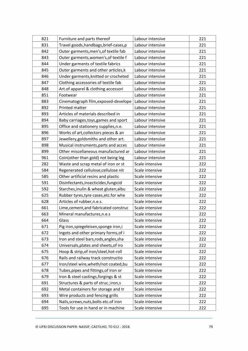
IE-UFRJ DISCUSSION PAPER: NASSIF; CASTILHO, TD 012 - 2018. 79
821 Furniture and parts thereof Labour intensive 221
831 Travel goods,handbags,brief-cases,p Labour intensive 221
842 Outer garments,men's,of textile fab Labour intensive 221
843 Outer garments,women's,of textile f Labour intensive 221
844 Under garments of textile fabrics Labour intensive 221
845 Outer garments and other articles,k Labour intensive 221
846 Under garments,knitted or crocheted Labour intensive 221
847 Clothing accessories of textile fab Labour intensive 221
848 Art.of apparel & clothing accessori Labour intensive 221
851 Footwear Labour intensive 221
883 Cinematograph film,exposed-develope Labour intensive 221
892 Printed matter Labour intensive 221
893 Articles of materials described in Labour intensive 221
894 Baby carriages,toys,games and sport Labour intensive 221
895 Office and stationery supplies,n.e. Labour intensive 221
896 Works of art,collectors pieces & an Labour intensive 221
897 Jewellery,goldsmiths and other art. Labour intensive 221
898 Musical instruments,parts and acces Labour intensive 221
899 Other miscellaneous manufactured ar Labour intensive 221
961 Coin(other than gold) not being leg Labour intensive 221
282 Waste and scrap metal of iron or st Scale intensive 222
584 Regenerated cellulose;cellulose nit Scale intensive 222
585 Other artificial resins and plastic Scale intensive 222
591 Disinfectants,insecticides,fungicid Scale intensive 222
592 Starches,inulin & wheat gluten;albu Scale intensive 222
625 Rubber tyres,tyre cases,etc.for whe Scale intensive 222
628 Articles of rubber,n.e.s. Scale intensive 222
661 Lime,cement,and fabricated construc Scale intensive 222
663 Mineral manufactures,n.e.s Scale intensive 222
664 Glass Scale intensive 222
671 Pig iron,spiegeleisen,sponge iron,i Scale intensive 222
672 Ingots and other primary forms,of i Scale intensive 222
673 Iron and steel bars,rods,angles,sha Scale intensive 222
674 Universals,plates and sheets,of iro Scale intensive 222
675 Hoop & strip,of iron/steel,hot-roll Scale intensive 222
676 Rails and railway track constructio Scale intensive 222
677 Iron/steel wire,wheth/not coated,bu Scale intensive 222
678 Tubes,pipes and fittings,of iron or Scale intensive 222
679 Iron & steel castings,forgings & st Scale intensive 222
691 Structures & parts of struc.;iron,s Scale intensive 222
692 Metal containers for storage and tr Scale intensive 222
693 Wire products and fencing grills Scale intensive 222
694 Nails,screws,nuts,bolts etc.of iron Scale intensive 222
695 Tools for use in hand or in machine Scale intensive 222

IE-UFRJ DISCUSSION PAPER: NASSIF; CASTILHO, TD 012 - 2018. 80
697 Household equipment of base metal,n Scale intensive 222
699 Manufactures of base metal,n.e.s. Scale intensive 222
722 Tractors fitted or not with power t Scale intensive 222
761 Television receivers Scale intensive 222
762 Radio-broadcast receivers Scale intensive 222
763 Gramophones,dictating,sound recorde Scale intensive 222
774 Electric apparatus for medical purp Scale intensive 222
775 Household type,elect.& non-electric Scale intensive 222
778 Electrical machinery and apparatus, Scale intensive 222
781 Passenger motor cars,for transport Scale intensive 222
782 Motor vehicles for transport of goo Scale intensive 222
783 Road motor vehicles,n.e.s. Scale intensive 222
784 Parts & accessories of 722--,781--, Scale intensive 222
785 Motorcycles,motor scooters,invalid Scale intensive 222
786 Trailers & other vehicles,not motor Scale intensive 222
793 Ships,boats and floating structures Scale intensive 222
885 Watches and clocks Scale intensive 222
233 Synth.rubb.lat.;synth.rubb.& reclai Specialized suppliers 223
711 Steam & other vapour generating boi Specialized suppliers 223
712 Steam & other vapour power units,st Specialized suppliers 223
713 Internal combustion piston engines Specialized suppliers 223
714 Engines & motors,non-electric Specialized suppliers 223
716 Rotating electric plant and parts Specialized suppliers 223
718 Other power generating machinery an Specialized suppliers 223
721 Agricultural machinery and parts Specialized suppliers 223
723 Civil engineering & contractors pla Specialized suppliers 223
724 Textile & leather machinery and par Specialized suppliers 223
725 Paper & pulp mill mach.,mach for ma Specialized suppliers 223
726 Printing & bookbinding mach.and par Specialized suppliers 223
727 Food processing machines and parts Specialized suppliers 223
728 Mach.& equipment specialized for pa Specialized suppliers 223
736 Mach.tools for working metal or met Specialized suppliers 223
737 Metal working machinery and parts Specialized suppliers 223
741 Heating & cooling equipment and par Specialized suppliers 223
742 Pumps for liquids,liq.elevators and Specialized suppliers 223
743 Pumps & compressors,fans & blowers, Specialized suppliers 223
744 Mechanical handling equip.and parts Specialized suppliers 223
745 Other non-electrical mach.tools,app Specialized suppliers 223
749 Non-electric parts and accessories Specialized suppliers 223
751 Office machines Specialized suppliers 223
752 Automatic data processing machines Specialized suppliers 223
759 Parts of and accessories suitable f Specialized suppliers 223
771 Electric power machinery and parts Specialized suppliers 223
772 Elect.app.such as switches,relays,f Specialized suppliers 223

IE-UFRJ DISCUSSION PAPER: NASSIF; CASTILHO, TD 012 - 2018. 81
773 Equipment for distributing electric Specialized suppliers 223
791 Railway vehicles & associated equip Specialized suppliers 223
271 Fertilizers,crude Science based. 224
512 Alcohols,phenols,phenol-alcohols,& Science based. 224
531 Synth.org.dyestuffs,etc.nat.indigo Science based. 224
532 Dyeing & tanning extracts;synth.tan Science based. 224
533 Pigments,paints,varnishes & related Science based. 224
541 Medicinal and pharmaceutical produc Science based. 224
551 Essential oils,perfume and flavour Science based. 224
553 Perfumery,cosmetics and toilet prep Science based. 224
554 Soap,cleansing and polishing prepar Science based. 224
562 Fertilizers,manufactured Science based. 224
598 Miscellaneous chemical products,n.e Science based. 224
764 Telecommunications equip and parts Science based. 224
776 Thermionic,cold & photo-cathode val Science based. 224
792 Aircraft & associated equipment and Science based. 224
871 Optical instruments and apparatus Science based. 224
872 Medical instruments and appliances Science based. 224
873 Meters and counters,n.e.s. Science based. 224
874 Measuring,checking,analysing instru Science based. 224
881 Photographic apparatus and equip Science based. 224
882 Photographic & cinematographic supp Science based. 224
884 Optical goods, n.e.s. Science based. 224
911 UN Special Code n.d 931 UN Special Code n.d 941 Animals,live, n.e.s.,incl. zoo-anima n.d 951 Armoured fighting vehicles, arms of n.d

IE-UFRJ DISCUSSION PAPER: NASSIF; CASTILHO, TD 012 - 2018. 82
Appendix 2
Trade Indicators
Revealed Comparative Advantage Index (Balassa, 1965)
𝑅𝐶𝐴 =
𝑋𝑖𝐵𝑅
𝑋𝐵𝑅⁄
𝑋𝑖𝑊
𝑋𝑊⁄
(A.1)
Where: 𝑋𝑖𝐵𝑅 corresponds to Brazilian exports of product i and 𝑋𝑊 corresponds to total
World exports.
Herfindal-Hrishmann Index
𝐻𝐻𝐼 = ∑ (𝑋𝑖𝑋⁄ )
2𝑛𝑖=1 (A.2)
Where: 𝑋𝑖corresponds to exports of product i and 𝑋 corresponds to total exports.
Intensive and Extensive margins of trade (Hummels and Klenow, 2005)
𝐼𝑀 =∑ 𝑋𝑗
𝐵𝑅𝑗∋𝑖
∑ 𝑋𝑗𝑊
𝑗∋𝑖
(A.3)
𝐸𝑀 =∑ 𝑋𝑗
𝑊𝑗∋𝑖
∑ 𝑋𝑖𝑊
𝑖
(A.4)
Where: j is the sub-set of i goods exported by Brazil (that can be named as the country’s
relevant export goods); 𝑋𝑗𝐵𝑅 corresponds to Brazilian exports of the sub-set of products j
and 𝑋𝑊 corresponds to total World exports (𝑋𝑗𝑊 is the world exports of product j and
𝑋𝑖𝑊is the total world exports). The IM correspond to the market share of Brazil for its
“relevant goods j”. The EM is the share of j products in total world exports.
Intra-industry Trade Index (Grubel-Lloyd, 1971)
+
−
−=
iii
iii
MX
MXGLI 1
(A.5)
IE-UFRJ DISCUSSION PAPER: NASSIF; CASTILHO, TD 012 - 2018. 83
Where: 𝑋𝑖 and 𝑀𝑖 correspond to a country’s exports and imports of product i.
For avoiding aggregation bias, we employed the 6-digit Harmonised System
disaggregation (around 5.000 product lines). Yet, trade flows are multilateral (not
geographically disaggregated).


![MILL’S HEDONISM · 2010] MILL’S HEDONISM 1707 not mainly because it is charitable but rather because, as I shall try to show, it fits the texts. Mill discusses these and related](https://static.fdocuments.us/doc/165x107/5af884c07f8b9abd588baded/mills-mills-hedonism-1707-not-mainly-because-it-is-charitable-but-rather-because.jpg)