HAL Id: halshs-00588309https://halshs.archives-ouvertes.fr/halshs-00588309

Preprint submitted on 22 Apr 2011

HAL is a multi-disciplinary open accessarchive for the deposit and dissemination of sci-entific research documents, whether they are pub-lished or not. The documents may come fromteaching and research institutions in France orabroad, or from public or private research centers.

L’archive ouverte pluridisciplinaire HAL, estdestinée au dépôt et à la diffusion de documentsscientifiques de niveau recherche, publiés ou non,émanant des établissements d’enseignement et derecherche français ou étrangers, des laboratoirespublics ou privés.

Trade integration and within-plant productivityevolution in ChileMaria Bas, Ivan Ledezma

To cite this version:Maria Bas, Ivan Ledezma. Trade integration and within-plant productivity evolution in Chile. 2008.�halshs-00588309�

WORKING PAPER N° 2007 - 09

Trade integration and within-plant productivity

evolution in Chile

Maria Bas

Ivan Ledezma

JEL Codes : F1, F4, O1 Keywords : trade barriers, plant productivity, firm

heterogeneity, plant-level data

PARIS-JOURDAN SCIENCES ECONOMIQUES

LABORATOIRE D’ECONOMIE APPLIQUÉE - INRA

48, BD JOURDAN – E.N.S. – 75014 PARIS TÉL. : 33(0) 1 43 13 63 00 – FAX : 33 (0) 1 43 13 63 10

www.pse.ens.fr

CENTRE NATIONAL DE LA RECHERCHE SCIENTIFIQUE – ÉCOLE DES HAUTES ÉTUDES EN SCIENCES SOCIALES ÉCOLE NATIONALE DES PONTS ET CHAUSSÉES – ÉCOLE NORMALE SUPÉRIEURE

Trade Integration and Within-Plant ProductivityEvolution in Chile∗

Maria BAS†and Ivan LEDEZMA‡

October 2008

Abstract

We study the impact of trade on productivity using Chilean plant-level data(1982-1999). Our contribution is to disentangle the impact of export and importbarriers. Firstly, we estimate the production functions to obtain plant TFP. Sec-ondly, we estimate trade barriers (border effects) between Chile and its tradingpartners at the industry level and over time. Finally, we test the impact of tradebarriers by regressing productivity on border effect estimates. A fall in export bar-riers improves productivity in traded sectors, while the reduction of import barriersmight foster productivity in export industries but it hurts firms in import-competingones.

Keywords: Trade barriers, plant productivity, firm heterogeneity, plant-leveldata.

JEL Classification: F1, F4 and O1.

∗We are grateful to Pol Antras, Jose Miguel Benavente, Gene Grossman, Thierry Mayer, JacquesMairesse, Nina Pavcnik, Andrea Repetto and James Tybout for helpful comments.

†Paris School of Economics & London School of Economics (Centre for Economic Performance). Email:bas@pse.ens.fr

‡Paris School of Economics & Universite Paris 1 Pantheon-Sorbonne (Centre d’Economie de la Sor-bonne). Email: ledezma@pse.ens.fr

1

1 Introduction

Trade liberalization was at the core of reform packages carried out in many developing

economies during the 1980s. In this paper we revisit the case of Chile, one of the earliest

and most radical examples of trade liberalization. We aim at testing the link between trade

integration and productivity in Chilean manufacturing plants. At the micro level, the

impact of trade reforms is generally studied from a unilateral perspective through direct

measures of trade costs or aggregate trade ratios that might neglect several features of

trade integration. The novelty of this paper is to estimate trade barriers in a multilateral

context to disentangle within a unique framework the effect of export- and import-oriented

policies on plant productivity.

By differentiating export and import trade barriers, we emphasize different channels

by which trade integration affects plant productivity. The reduction of import barriers

increases foreign competition, which is often viewed as a positive engine of productivity

(Pavcnik, 2002; Amiti and Konings, 2007). It pushes the least productive firms to cease

production and surviving ones to trim down their inefficiencies. On the other hand,

the presence of increasing returns to scale and imperfect competition may modify the

relationship between import competition and plant productivity (Devarajan and Rodrik,

1989; Rodrik, 1988). One consequence of scale economies is precisely that average cost falls

as output increases. In this case, foreign competition reduces domestic sales restricting

the possibility to exploit scale economies.

Import-oriented policies also determine the extent of foreign technology transmissions.

In developing countries, the access to high-quality imported capital equipment or inter-

mediate goods enables firms to reduce their marginal costs and to raise their productivity

level. Using plant-level data, Schor (2004) for Brazil, and Amiti and Konings (2007) for

Indonesia show that input tariff reductions boost productivity gains.1

On the other hand, export promotion policies allow more firms to benefit from positive

spillovers stemming from foreign markets. The literature suggests learning-by-exporting

1Kasahara and Rodriguez (2008) for Chile, find that imported inputs foster plant productivity.

2

as a plausible mechanism to explain a positive impact of trade liberalization on plant

productivity. There is some evidence on ex-post productivity gains arising from knowledge

and expertise gained in the export process (Kraay (2002) on China, Alvarez and Lopez

(2005) on Chile, De Loecker (2007) on Slovenia).

These different mechanisms of trade liberalization call for further analysis on the

multiple dimensions of trade. We carry out three empirical exercises. Firstly, we obtain

estimates of plant TFP and address simultaneity issues thanks to the Levinsohn and

Petrin (2003) methodology. These estimates draw on plant-level data (1979-1999) from

the annual industry survey ENIA (Encuesta Nacional Industrial Anual) of the Chilean

manufacturing sector provided by the INE (Instituto Nacional de Estadisticas). Secondly,

we use specific data on destination markets for bilateral trade flows of Chile and its

main trade partners at the industry level to capture (a) the barriers faced by Chilean

partners to reach the domestic market (import barriers) and (b) those barriers faced by

Chilean exporters to access foreign markets (export barriers). To estimate these barriers

we rely on the border effect methodology developed by Fontagne et al. (2005) and use the

Trade and Production database provided by the CEPII (Centre d’Etudes Prospecives et

d’Information Internationales). This strategy enables us to obtain time-varying measures

of trade integration at the industry level. Unlike Chilean tariff rates, these measures do

present heterogeneity across industries. Finally, we estimate the impact of import and

export barriers on plant productivity by combining the results of the first two steps. In

this third step, we regress plant productivity on border effect estimates.

We carried out several robustness checks. We use alternative measures of productivity,

different specifications dealing with potential mark-ups bias and dynamic concerns of the

persistence of plant productivity over time. In the different empirical stages we deal with

the potential risk of reversal causality between trade barriers and plant productivity. This

is done by purging productivity effects in the gravity specification, by using a four-year

rolling horizon in step 2 and by treating trade barriers as endogenous in GMM estimations.

We also test two possible mechanisms by which trade affects plant productivity, namely

3

the presence of IRS and foreign technology transmission.

Based on specific trade barrier measures, the paper yields new findings on trade policy

implications. Considering productivity gains relative to non traded sectors, our regressions

suggest three main results: (i) a reduction in export barriers fosters plant productivity

gains in export-oriented and import-competing industries; (ii) the impact of import bar-

riers depends on trade orientation. A decrease in import barriers has a negative effect

on plant productivity in import-competing industries. Interestingly, production function

estimates suggest the presence of increasing returns to scale (IRS) in these industries. For-

eign competition may have dampened domestic sales and thereby, reduced the possibility

to exploit scale economies. Concerning export-oriented industries, a fall in import barriers

fosters plant productivity. This result is present in different static specifications. However,

once we control for past productivity levels in the dynamic model, foreign competition

might also reduce productivity gains in these industries; (iii) a reduction in import barriers

on machinery improves plant productivity of both export-oriented and import-competing

industries.

Our findings contribute with new evidence on trade liberalization and plant produc-

tivity in Chile. The identification setting has been chosen to allow for a close comparison

with previous results obtained by Pavcnik (2002) and Bergoeing et al. (2006).2 Both stud-

ies show the presence of time-varying firm heterogeneity and deal with the effects of trade

integration on productivity gains in a similar and comparable indentification strategy. Us-

ing plant-level data, Pavcnik (2002) estimates the impact of trade on plant productivity in

Chile during the period 1979-1986. By the means of a difference-in-difference framework,

Pavcnik (2002) concludes that trade liberalization induces the growth of within-plant pro-

ductivity in import-competing industries. Productivity improvements in export-oriented

industries are observed only for initial years.3 Using our sample, we are able to repro-

2Several works have investigated the relationship between Chilean market-oriented reforms and plantproductivity. See Liu and Tybout, 1996; Pavcnik, 2002; Bergoeing et al., 2002; Bergoeing et al., 2004;Alvarez and Lopez, 2005; Bergoeing et al., 2006.

3Pavcnik (2002) also performs the Olley and Pakes (1996) aggregate productivity decomposition andshows that, in the period, aggregate productivity growth is mainly explained by the exit of the leastproductive firms and the reallocation of market shares towards most productive ones.

4

duce these results. However, contrary to what the difference-in-difference specification

assumes, trade exposure in Chile does not increase continuously during Pavcnik’s sample

period. In the context of the 1982 debt crisis, the government raises import tariffs from

15% in 1982 up to 26% in 1985.

Chilean trade reforms have been recently revisited by Bergoeing et al. (2006). They

study the impact of the financial and trade reforms on productivity gains in Chile during

a longer period (1980-2001). The authors show that if one uses effective tariffs instead

of year dummies to capture trade liberalization, plant productivity advantages in export-

oriented industries are not significant and, similar to our results, productivity gains of

plants belonging to import-competing industries fall after trade liberalization.

Nevertheless, both studies suffer from the lack of cross-section variance on the right-

hand side of regressions. Indeed, the identification of trade liberalization effects can be

problematic since the reduction in import tariffs was almost homogeneous across industries

and remained constant during the 1990s. The radical drop in the average nominal tariff

rate from 98% in 1973 to 10% in 1979 came along with the homogenization of tariff rates

among industries. Even their rise in early 1980s, during the debt crisis, was uniform. This

homogeneous tariff reduction is probably the reason why Pavcnik (2002) is constrained

to use time dummy indicators and Bergoeing et al.(2006) can not get enough variance for

their estimates concerning export-oriented industries.

Considering direct measures of trade policy such as import tariffs also neglects two

important features of trade integration. First, a unilateral import tariff reduction does

not necessarily imply a symmetric response across trade partners. Second, several direct

and indirect trade barriers might be omitted (Anderson and van Wincoop, 2004). Among

them, one finds not only non-tariff barriers and fixed export costs, but also bilateral agree-

ments, institutional arrangements, infrastructure and even political efforts. For instance,

while the evolution of tariffs in Chile remains flat during the 1990s, in order to promote

exports the government signed several trade agreements with different countries and also

developped an important agenda of political integration.

5

By estimating the evolution of trade integration between Chile and its trading partners,

we are able to capture this type of missing information. This strategy also allows us to

address the lack of cross-section variance of standard trade measures and to capture

the multiple channels of trade integration. These are the main contributions relative to

previous works.

The rest of the paper is structured as follows. Section 2 presents the estimation

strategy of our empirical exercises. Section 3 shows the results and, finally, section 4

presents a brief conclusion.

2 Estimation strategy

The estimation strategy consists of three steps. In the first one, we estimate the production

function using OLS, fixed-effect specification and the LP methodology to obtain plant

TFP as a residual. In the second step, we construct the measure of trade liberalization

by estimating border effects between partners following Fontagne et al. (2005). Finally,

in the third step, we estimate the impact of trade barriers by regressing productivity on

border effect estimates. Within this methodology, we address simultaneity issues in the

estimation of TFP (step 1) and reversal causality between productivity and trade flows

(step 2 and 3).

2.1 Step 1: Production function

We estimate the following specification of a Cobb-Douglas production function at the

two-digit industry level:

ypt = β0 + βxxpt + βkkpt + εpt (1)

Where all variables are expressed in natural logs, ypt is the value added of plant p at

time t, which is explained by short-term adjustable inputs xpt (i.e. skilled and unskilled

labor) and capital stock kpt. The error term can be decomposed into an intrinsical ”trans-

mitted” component ωpt (productivity shock) and an i.i.d. component χpt. Consequently,

6

plant TFP apt is calculated as the residual given by the difference between the observed

output and the predicted factor contribution:

apt = ypt − βxxpt − βkkpt (2)

When estimating production functions using firm panel data, eventual problems con-

cerning simultaneity and selection should be considered. Simultaneity arises because input

demand and unobserved productivity are positively correlated. Firm specific productivity

is known by the firm but not by the econometrician. If a firm expects a high productivity

shock it will anticipate an increase in its final good demand and, consequently, it will

purchase more inputs. OLS will tend to provide upwardly biased estimates of the labor

elasticity and downwardly biased estimates of the capital one4. Selection problems are

likely to be present because the unobserved productivity influences the exit decision of

the firm and we can only observe those firms that stay in the market. On the other hand,

if capital is positively correlated with profits, firms with larger capital stock will decide

to stay in the market even for low realizations of productivity shocks. This implies a

potential source of negative correlation in the sample between productivity shocks and

capital stock, which translates into a downward bias in capital elasticity estimates.

Olley and Pakes (1996) (henceforth OP) propose a three-stage methodology to con-

trol for the unobserved firm productivity. They deal explicitly with exit and investment

behavior. The rationale is to reveal the unobserved productivity through the investment

behavior of the firm, which in turns depends, theoretically, on capital and productivity.

Selection issues are taken into account by inferring that firms that stay in the market have

decided to do it accordingly to their capital stock and their expectations of productivity.

By the means of this theoretical exit rule, OP estimate survival probabilities conditional

on firm’s available information. These probabilities are then used in the productivity

4OLS elasticities can be stated as βx = βx + σkkσxε−σxkσkε

σxxσkk−σ2xk

and βk = βk + σxxσkε−σxkσxε

σxxσkk−σ2xk

. Where σrs

is the covariance between variables r and s in the sample. If capital is positively correlated with laborand labor’s correlation with the productivity shock is higher than capital one (which is the realistic case)then the coefficient of capital βk will be underestimated and the one of labor βx upward biased.

7

estimation.

Levinsohn and Petrin (2003) (henceforth LP) extend the OP idea, by noting that some

inputs, such as electricity or materials, can be better proxies than investment to control

for the unobserved firm productivity when one deals with simultaneity. Inputs adjust

in a more flexible way, so they are more responsive to productivity shocks. Moreover,

inputs usually have more non-zero observations than investment, a property that has

consequences on estimation efficiency. In the case of the ENIA survey this property is

important. Thus, in order to maximize sample size we keep the LP strategy and use

electricity as a proxy for unobserved productivity.5

There are some advantages of OP-LP methodologies. Firstly, they perform better

than fixed-effect specifications because the unobserved individual effect (productivity) is

not constrained to be constant over time. Secondly, approaches based on instrumental

variables can be limited by the instruments availability. Finally, OP-LP do not assume

restrictions on the parameters. For instance, an alternative approach is the one developed

by Katayama et al.(2005) who show how misleading can be the use of sale revenues to

measure productivity. Factor prices and mark-ups can produce important distortions if

they are not homogeneous. However, their methodology assumes constant returns to scale

and neglect entry-exit process to facilitate likelihood estimates. Again both assumptions

are not neutral in the case of the ENIA. In the third step, we allow for plant’s individual

fixed effects and control for market concentration at a disaggregated industry level in

order to reduce the potential risk of mark-up bias.

2.2 Step 2: Border effects

It is well known that the reduction of tariffs in Chile was homogeneous across industries.

As a consequence, tariff rates do not provide enough cross-section variance. On the other

hand, tariffs are not the only measure that matters to capture trade costs. One should also

5Besides technical concerns, a key difference between LP and OP is that the former does not directlytake into account selection. However, as LP show, the risk of selection biases are significantly reduced byconsidering an unbalanced panel.

8

consider bilateral agreements, asymmetries between export and import costs and indirect

difficulties to trade.6 Considering all these features of trade, we do obtain heterogeneity

in both industrial and time dimensions.

To do so, we apply a border effect methodology. This type of empirical strategy

provides an assessment of the level of trade integration by estimating a gravity-like model

that considers, as a very intuitive benchmark, the market access of domestic producers

reaching domestic (intra-border) destinations. 7

2.2.1 The Methodology

The identification strategy of Fontagne et al.(2005) builds on Head and Mayer (2000)

gravity model derivation. This strategy seems suitable to measure Chilean trade integra-

tion as it corrects for the lack of theoretical foundations of earlier works and keeps the

idea of using intra-national trade as a benchmark of trade integration. Moreover, it allows

for asymmetries in the identification of trade barriers among partners, one of the main

focus of this paper. Fontagne et al.’s (2005) theoretical foundation builds on a static mo-

nopolistic competition setting with increasing returns to scale for one-sector economies.

Consider an instantaneous CES utility function in which the representative consumer of

country i has specific preferences asijt for each variety h depending on the exporter country

j (for the sake of clarity in the exposition of our empirical implementation, we indicate

explicitly both industry s and time t specificity):

U sit =

Nst∑

j=1

Msjt∑

h=1

(as

ijtcsijht

)σt −1σt

σt

σt −1

(3)

Thus, varieties belonging to the same country share the same weight in the utility

6Theoretically, these indirect difficulties include a large list of country specificities, namely bias ofconsumption towards home goods and the like. As long as they can be interpreted, at least in part, asthe outcome of history and political efforts, we consider them as a part of the measure of trade integration.

7McCallum (1995) applies this methodology to study market access between Canada and the US.Despite the high expected trade integration, trade between US and Canada is found to be around 22times more difficult than Canadian intra-national trade. Anderson and van Wincoop (2003) reestimateMcCallum’s (1995) model, correcting for multilateral price bias, and the assessment still remains striking(11%).

9

function. Imports msijt(= cs

ijtpsijt) of country i from country j are valuated at the point of

consumption (c.i.f) psijt = ps

jtτsijt . This includes the producer price (f.o.b.) ps

jt augmented

of all trade cost τ sijt, modeled as iceberg costs. Total expenditure for the industry Y s

it =Ns

t∑j′=1

msij′t considers all imports, including intra-national ones ms

iit. For symmetric varieties,

this utility function (3) with constant elasticity σt leads to the well known demands:

msijt =

(ps

jtτsijt

asijtP

sit

)1−σt

M sjtY

sit (4)

In this gravity-like equation (4), P sit =

[Nt∑

j′=1

(pij′taij′t

)1−σt

M sj′t

] 11−σt

is the consumer price

of all varieties in the industry. This index takes into account differences in price setting

across countries. If omitted, not only a multilateral control is missing but also a bias is

induced between the error term and the partners dummies (border effect). Anderson and

van Wincoop (2003) argue that the omission of multilateral price effects (what they call

”multilateral resistances”) explains the upward bias in border effects of Canada vis-a-vis

the US estimated by McCallum (1995).8

One might mention four possible strategies to consistently estimate a gravity equation

including price effects. The first one is to use price index data. Baier and Bergstrand

(2001) follow this strategy measuring prices with GDP deflators. However, as highlighted

by Anderson and van Wincoop (2004), empirical counterparts of P sit such as CPIs mea-

sures neglect changes in the true set of varieties and do not accurately reflect non tariff

barriers and indirect trade policies. The second strategy is the one followed by Anderson

and van Wincoop (2003). They develop a two-step methodology in which border effect

estimates are used to measure multilateral price effects. Besides practical difficulties of

implementation, one crucial limitation for our purposes is the assumption of symmetry

in bilateral trade costs. A third alternative approach uses fixed effect specification to

control for unobservable prices. The effect of price indexes is captured by the coefficients

of individual fixed effects related to country source and destination (Harrigan, 1996).

Feenstra (2003) shows that the coefficients of fixed effect estimation are consistent and

8See previous footnote

10

reports values very similar to the non-linear least squares estimation of Anderson and

van Wincoop (2003). Redding and Venables (2004) construct market access measures to

explain cross-country differences in per capita income. Their market access estimation

relies on fixed country effects to capture exporting and importing country characteristics.

These country indicators take into account unobserved economic variables associated with

supply and market capacity.

If the economic and geographic determinants captured by fixed effects vary over time,

a useful strategy consists in eliminating the price index in the CES demand setting by

expressing inter-national imports relative to intra-national ones. This is what Head and

Mayer (2000) do. We follow this solution and divide equation (4) by msiit:

msijt

msiit

=

(as

ijt

asiit

)σt−1 (ps

jt

psit

)−σt(

τ sijt

τ siit

)1−σt(

vsjt

vsit

)(5)

Wherevs

jt

vsit

is the relative value added at industry level between both countries (i and

j).The relative value added captures the relative number of symmetric varieties within a

model of monopolistic competition. To obtain an empirical counterpart of equation (5),

we assume, as Fontagne et al. (2005), that trade costs (τ sijt) are composed of transport

cost (captured by distance dij), ad-valorem tariffs (tsijt) and ”tariff equivalent” (NTBsijt)

of non tariff barriers: τ sijt ≡ (dij)

δt (1 + tsijt) (

1 + NTBsijt

).

Protection (tariffs and non tariff barriers) varies across all partner pairs and depends

on the direction of the flow for a given pair. To capture this, a dummy structure is defined

to take into account flows’ direction. Taking the example of the US and Chile as trade

partners we define(1 + tsij

) (1 + NTBs

ijt

)≡ exp

[ηs

t US CHLsijt + γs

t CHL USsijt

], where

US CHLsijt is a dummy variable set equal to 1 when Chile is the exporter country j and

the US the importer country i. Similarly, CHL USsijt is a dummy variable set equal to 1

when the US is the exporter country j and Chile the importer country i.

Preferences asijt are supposed to have a random component es

ijt and a systematic bias

βsit for goods produced in the home country i. This ”‘home market bias”’ is reduced when

countries i and j share the same language and are contiguous. The dummies Lij and Cij

11

are defined to capture each situation, respectively. Under these assumptions preferences

can be written as asijt ≡ exp

[es

ijt − (βsit − λLtLij − λCtCij)

(US CHLs

ijt + CHL USsijt

)],

where λLt and λCt represent the extent to which the home market bias is mitigated by

common language and contiguity. Taking into account these assumptions, equation (5),

for the example of the US and Chile, can be written as:

ln

(ms

ijt

msiit

)= ln

(vs

jt

vsit

)− (σt − 1) δt ln

(dij

dii

)− (σt − 1) λLtLij − (σt − 1) λCtCij (6)

−σt ln

(ps

jt

psit

)− (σt − 1) (βs

it + ηst ) US CHLs

ijt − (σt − 1) (βsit + γs

t ) CHL USsijt

+ (σt − 1)(es

ijt − esiit

)2.2.2 Empirical specification

The number of observations in our international sample does not allow to split the sample

by each year and 2-digit industry. In order to consistently estimate equation (6), we run

pooled regressions in a four-years rolling window for each industry. This allows us to

obtain time-varying elasticities. Our estimable equation can be written as:

ln

(ms

ijt

msiit

)= α1t′ ln

(vs

jt

vsit

)+ α2t′ ln

(dij

dii

)+ α3t′Lij + α4t′Cij + α5t′ ln

(ps

jt

psit

)(7)

+α6t′US CHLsijt + α7t′CHL USs

ijt + εijt

Where the theoretical counterparts of each α1t′ , α2t′ , .., α7t′ are given by equation (6).

We split the sample by each 2-digit industry and sample periods t = t′ − 3 to t′ , where

t′ runs from 1982 to 1999. In this sense, α6t′ and α7t′ will capture the average border

effects of exports of Chile to the US and imports of Chile from the US, respectively

(i.e. − (σt − 1) (βsit + ηs

t ) and − (σt − 1) (βsit + γs

t )) during the period t′ − 4 to t′. In the

regressions, we drop the constant and incorporate all dummy variables to capture the

partners in each trade flow direction (i.e. US CHLsijt and CHL USs

ijt in our example

of Chile and the US ). Thus, α6t′ can be directly interpreted as the export border effect

12

(Chilean exports to the US) and α7t′ as the import border effect (US imports to Chile).

We run OLS regressions and, due to the form of the error term, εij = (σ − 1) (eij − eii) , we

use Hubert and White corrected standard errors clustered at the importer-industry-year

level to control for the expected correlation. In equation (7) we do not impose α1t′ = 1,

as the theoretical equation (6) suggests, and allow for its empirical estimation.

Note that a potential endogeneity problem exits in the estimation of equation (7).

In a monopolistic competition framework, prices and output are determined simultane-

ously. Fontagne et al. (2005) use aggregate prices (instead of industry-level ones). The

underlying assumption is that prices at the national level are less correlated with profit

maximization at the firm level. In our estimation, we adopt a different approach and use

relative wages at the industry level. This choice is motivated by the potential reverse

causality in Step 3. As previously mentioned, we will use the border effect estimates to

test the impact of trade liberalization on plant productivity for different industries. Most

productive industries (or those producing high quality goods) will tend to increase their

trade flows and induce a downward bias in the border effect estimates (Step 2). Our as-

sumption is that relative wages capture potential asymmetries in technology or efficiency

and thereby they help to remove productivity concerns from the border effect estimates.9

Additionally, due to the four-year rolling horizon the border effect estimates include past

values of trade flows, which allows for a lagged effect of the change in trade barriers. This

also contributes to reduce the risk of reversal causality in Step 3.

From these industry-level estimations, we obtain the border effects from the dummy co-

efficients corresponding to each combination of partners and trade flows direction (α6t′ and

α7t′ ). In our regressions we consider bilateral trade flows of all main trade partners of

Chile. The list includes the US, 9 European countries (EU) and 7 Latin American coun-

tries (LA) including Chile (See section 3). Border effects are captured by the bilateral

dummies indicating all combination of flows between the EU, LA, the US and Chile. This

structure also captures the difference between trade barriers among partners belonging

9In non-reported regression we have used relative aggregate prices and also the lag of relative aggregateprices and relative wages. The resulting border-effect estimates are very close to those used in whatfollows.

13

to the same region.10 Finally, our proxies of export and import barriers are constructed

for each industry as the weighted average of the border effects estimated for all partners.

Weights are given by the part of the import (export) flow on total imports (exports) of

Chile.

2.3 Step 3: The impact of trade policy on plant TFP

In this final step, we use the previous estimates of trade barriers to measure the impact

of trade liberalization on plant productivity across export-oriented and import-competing

industries relative to non-traded ones. The following reduced equation is estimated, anal-

ogous to the difference-in-difference framework implemented by Pavcnik (2002):

apt = θ0 + β Bpt + ζ Tp + δ Bpt · Tp + ϕ Zpt + ξpt (8)

Where θ0 is the constant and ξpt the error term. apt is the log of TFP of plant p at

time t estimated by the LP strategy. Bpt is a vector of trade barriers estimates (import

and export border effects) for the 2-digit industry in which the plant operates. Tp is a

vector of trade orientation dummies indicating if the plant belongs to export-oriented or

import-competing industries. Similar to Pavcnik (2002), we classify industries by trade

orientation at the 3-digit industry level (See Appendix). Plants are classified as export-

oriented if they belong to a 3-digit industry which has more than 15% of exports over total

production and as import-competing if the industry has more than 15% of imports over

total production. The rest are considered as non-traded. 11 Our classification concerns the

initial period of 1980-1986. The initial sample classification also helps to avoid endogeneity

10Following our notation the set of dummies for the EuropeanUnion (EU), Latina America (LA), Chile (CHL) and the US (US) is:EU CHLs

ijt, CHL EUsijt, US CHLs

ijt, CHL USsijt, EU EUs

ijt, LA CHLsijt, CHL LAs

ijt,LA LAs

ijt, EU LAsijt, LA UEs

ijt, LA USsijt, US LAs

ijt, EU USsijt, US EUs

ijt.

11There are only two industries (351 and 384) that matched up to both categories. Nevertheless, theindustry 351 (384) presents an export-output ratio of 0.82 (0.21) and an import-output ratio of 1.32(2.01). Therefore these industries were classified as import competing. Our results remain unchanged ifwe consider a fourth category of export-import competing for industries 351 and 384 (See the technicalappendix).

14

problems arising from the classification. As Pavcnik (2002) notes, classification at 3- or

4-digit does not change significantly. Neither does it when considering the pre-sample

period.

Zpt is a vector of plant characteristics: industry affiliation at 2-digit 12, indicators of

entry and exit and plant characteristics that may change over time, namely the use of

imported inputs and credit constraints. Similar to Bergoeing et al. (2006), we identify

plants that may face liquidity constraints using as a proxy a loan tax payment at the plant-

level. In Chile, financial credits are subject to this tax. ”‘Credit”’ is a dummy variable

equals to one if the plant reports having paid this tax in a given year. This information

is used as a signal that the plant has not been financial constraint. We also introduce

year indicators to control for other macroeconomic shocks. The excluded categories are

non-traded industries, the year 1982 and the industry 38. As a robustness check we use

alternative measures of plant productivity and also control for variable mark-ups.

We are mainly interested in the estimates of the vector coefficient δ of the interaction

terms ( Bpt · Tp). Negative and significant coefficients mean that a reduction of trade

barriers has a positive effect on productivity in traded industries (export-oriented and

import-competing) relative to non-traded ones. The full set of interaction terms enables

us to measure separately the effect of import and export barriers, depending on trade

orientation.

2.4 Data

In the first step, we use plant-level data from the ENIA survey, which is provided by the

Chilean institute of statistics INE (Instituto Nacional de Estadisticas). This survey is a

manufacturing census of Chilean plants with more than 10 employees. Our data covers the

period 1979-1999 and contains information of added value, materials, labor, investment

12We introduce industry indicators in order to control for specific characteristics of industries. In orderto avoid possible colinearity issues, following Pavcnik (2002), the industry affiliation dummies are definedat the 2 digit industry level, while trade orientation dummies are defined at the 3 digit industry level.

15

and exports (only available from 1990).13 We used different specific deflators at the 3-digit

level (ISIC Rev-2) and year base 1992 for added value, exports, materials and investment.

For the latter, specific deflators are considered for infrastructure, vehicles and machinery.

Capital series were constructed using the methodology of Bergoeing et al. (2006).14 Table

7 (Appendix) shows a description of the variables and Table 8 (Appendix) reports general

descriptive statistics of the plant-level sample.

In the second step we use data from the ”‘Trade and Production Database”’ con-

structed by CEPII (Centre d’Etudes Prospecives et d’Information Internationales). This

is an extension of the data collected by Nicita and Olarreaga (2001) at the World Bank.

The CEPII has filled many missing values for production variables using UNIDO and

OECD-STAN (for OECD members). It has also completed trade data with the interna-

tional trade database BACI of CEPII. The final bilateral trade data covers the period

1976-1999 for 67 developing and developed countries. It provides information on value

added, export and import trade flows, origin and destination countries, wages and labor

at the 3-digit industry level (ISIC Rev-2).

Detailed intra-national trade flows for our sample of countries are not available. Intra-

national trade is computed as output minus exports. This requires an appropriate measure

of internal distance that should take into account economic activity to weight internal

regions (Head and Mayer, 2000). For distance variables, contiguity and common language,

we also used the CEPII database of internal and external distances. The CEPII uses

specific city-level data in order to compute a matrix of distance including the geographic

population density for each country. Distance between two countries is measured based on

bilateral distance between cities weighted by the share of the city in the overall country’s

population.

At the end, bilateral trade data is available for nine members of the European Union

throughout the whole period 1979-1999 (Germany, France, Great Britain, Italy, Belgium,

Luxembourg, Ireland, Netherlands and Denmark), the United States and seven Latin-

13The ENIA survey has been used in previous studies such as Pavcnik (2002), Liu and Tybout (1996),Levinsohn and Petrin (2003) and Bergoeing et al. (2006) for different sample periods.

14We thank the authors for providing us with their Stata routine for capital series.

16

American countries (Argentina, Brazil, Bolivia, Chile, Mexico, Uruguay and Venezuela).

3 Results

3.1 Results of step 1: plant TFP estimates

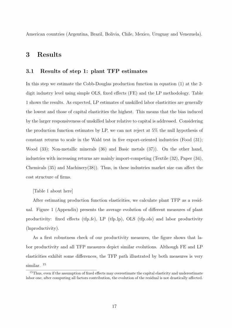
In this step we estimate the Cobb-Douglas production function in equation (1) at the 2-

digit industry level using simple OLS, fixed effects (FE) and the LP methodology. Table

1 shows the results. As expected, LP estimates of unskilled labor elasticities are generally

the lowest and those of capital elasticities the highest. This means that the bias induced

by the larger responsiveness of unskilled labor relative to capital is addressed. Considering

the production function estimates by LP, we can not reject at 5% the null hypothesis of

constant returns to scale in the Wald test in five export-oriented industries (Food (31);

Wood (33); Non-metallic minerals (36) and Basic metals (37)). On the other hand,

industries with increasing returns are mainly import-competing (Textile (32), Paper (34),

Chemicals (35) and Machinery(38)). Thus, in these industries market size can affect the

cost structure of firms.

[Table 1 about here]

After estimating production function elasticities, we calculate plant TFP as a resid-

ual. Figure 1 (Appendix) presents the average evolution of different measures of plant

productivity: fixed effects (tfp fe), LP (tfp lp), OLS (tfp ols) and labor productivity

(lnproductivity).

As a first robustness check of our productivity measures, the figure shows that la-

bor productivity and all TFP measures depict similar evolutions. Although FE and LP

elasticities exhibit some differences, the TFP path illustrated by both measures is very

similar. 15

15Thus, even if the assumption of fixed effects may overestimate the capital elasticity and underestimatelabor one, after computing all factors contribution, the evolution of the residual is not drastically affected.

17

3.2 Results of step 2: Border effect estimates

In the second step, we construct market access measures by estimating equation (7) at the

2-digit industry level. This estimation captures the heterogeneity of trade barriers across

industries. Figure 2 (Appendix) plots the weighted average of export and import border

effect estimates across trade partners. Weights are based on each country export (import)

share over total exports (imports) of Chile. All coefficients are significant at least at 5%.

The solid line depicts export border effects and the dashed line those corresponding to

import.

Difficulties of Chilean exporters to access foreign markets (export border effect) were

relatively constant at the beginning of the eighties. Reflecting the active trade agreement

agenda, most industries switch to a downward trend at the end of the 1980s. This be-

comes specially pronounced during the 1990s. This is the case of Wood, Textiles, Plastics

and Machinery. Two important export-oriented industries, Basic metals and Food, show

an evolution of export border effect almost flat. The former, however, is the most tradi-

tional export-oriented industry and in this industry trade barriers were already low at the

beginning of the period. On the other hand, the rather flat evolution of export barriers

on Food industry might be explained by quality controls set by EU and the US. Home

biases are also likely to be present in this type of industry. Once again one observes the

extent to which direct trade measures such as import tariffs do not capture all dimensions

of trade integration: export barriers have considerably diminished in all industries during

the 1990s, even if import tariffs were already low.

Figure 2 also shows the evolution of the weighted measure of industry-level barriers

faced by EU, LA and the US to access the Chilean market (import border effect). In many

industries, import barriers increased during the first half of the 1980s (Food, Textiles,

Wood, Non-metallics and Machinery). This is consistent with the raise in import tariffs

during this period and also with other discretionary policy measures set to control the

current account deficit during the debt crisis. Since we use a moving average of border

effects, this tendency is observed even in the late 1980s as a lagged effect of protection.

18

During the 1990s import border effects fall in almost all industries except in Basic metals.

This reduction and convergence of import border effects seem also consistent with the new

trade integration agenda of Chile based on bilateral and multilateral trade agreements.

3.3 Results of step 3: The impact of trade barriers on plant

TFP

The final step consists in identifying the influence of each type of trade barrier on the

evolution of plant productivity. Equation (8) disentangles the variation in productivity

due to changes in trade barriers depending on trade orientation. We are interested in the

vector coefficient δ of the interaction terms between trade orientation indicators and our

border effect estimates.

3.3.1 Reproducing Pavcnik’s (2002) results

In order to provide a baseline estimation, we start by reproducing Pavcnik’s (2002) regres-

sions for our full sample period. We use within group estimates in a difference-in-difference

framework. In this specification, year indicators capture trade liberalization effects. These

estimates are illustrated in Figure 3 (Appendix). We obtain similar results to Pavcnik

(2002). Once controlling for exit and plant specific characteristics, trade liberalization

(captured by time dummies) has a positive impact on plant productivity in traded indus-

tries (export-oriented and import-competing) relative to non-traded ones. Interestingly,

considering only the period 1980-1986, Pavcnik (2002) highlights that plant productivity

gains in export-oriented industries are minor. Using the full sample period, this trend

changes after the 1990s.

3.3.2 Disentangling the effects of export and import barriers

In this section, we employ the weighted average border effects estimated in step 2. As pre-

viously mentioned, we use a four-year rolling window for each industry. Hence, the border

effect measures capture not only the current but also the lagged effect of trade integration

19

on plant TFP. This implies the loss of initial years in the sample (1979-1981). On the

other hand, these lagged measures of border effects and the controls introduced in step 2

to address asymmetric technologies reduce the risk of potential endogeneity between our

measure of trade barriers and productivity. Additionally, in robustness check of dynamic

specification we treat border effects as endogenous regressors in GMM estimations.

Table 2 reports the results using the plant TFP measured by the LP methodology

(TFP LP). After controlling for industry specific effects (2-digit industry indicators) and

macroeconomic shocks (year indicators), the coefficients of the other variables should

only capture the effects of within-industry productivity variation. We consider plant-

fixed effects and use Huber-White standard errors in all estimations. In the last column,

these errors are corrected for clustering at the plant level.

The first column presents the baseline estimation. In this specification we include

the indicators for export-oriented (Export) and import-competing (Import) industries,

the measures of import border effects (BM) and export border effects (BX) and their

interactions (Export*BX, Import*BX, Export*BM, Import*BM). In this difference-in-

difference framework we interpret the coefficients of interaction terms relative to non-

traded industries (the omitted category). Export border effects interacted with both

export-oriented (Export*BX) and import-competing (Import*BX) indicators present a

negative and significant coefficient. This suggest a positive and significant impact of

export barrier reductions on plant productivity in both traded industries. This result can

be related to learning-by-exporting and international knowledge spillovers (Kraay (2002)

on China, Alvarez and Lopez (2005) on Chile and De Loecker (2007) on Slovenia). In

the case of plants belonging to import-competing industries, the positive effect of export

barrier reductions on their productivity could be driven by new-exporters within these

industries. Bergoeing et al.(2005) show that, even if with a small aggregate export share, a

number of plants entered the export market during the nineties in those Chilean industries.

The impact of import barriers depends on trade orientation. We find evidence of a

negative effect of import barrier reductions on productivity of plants belonging to import-

20

competing industries (Import*BM). Therefore, contrary to Pavcnik’s (2002) results, in our

regressions foreign competition appears to dampen plant productivity in those industries.

The production function estimates (step 1) show that import-competing industries (Tex-

tile, Paper, Chemicals and Machinery) operate under increasing returns to scale (IRS).

In this case, import competition reduces market shares of domestic firms shrinking the

opportunities to exploit scale economies. This possible explanation has also been em-

phasized by Bergoeing et al. (2006) for different production function estimates and data

treatment.

[Table 2 about here]

On the other hand, the reduction of import barriers has a positive impact on plant

productivity in export-oriented industries (Export*BM). While import competition does

not affect export sales, exporters also sell in the domestic markets and have to face foreign

competitors. Hence, this category of exporters may help to isolate the ”trimming fat”

effect of foreign competition, since economies of scale are guaranteed for these firms by the

access to international markets. The positive effect of the reduction of import barriers on

plant productivity in export-oriented industries, in these static regressions, might come

from innovative strategies implemented to improve domestic competitiveness. However,

if one might expect a positive and a negative effect of foreign competition, for plants

belonging to import-competing industries the effect of market size reduction is negative

enough to offset a positive outcome of import barrier reductions.

The above results (interaction terms) remain almost unchanged after the progressive

inclusion of several controls. 16 As expected, the exit indicator (Exit ind) has a neg-

ative coefficient (column (2)). Exiting plants are on average 14% less productive than

surviving plants. The entry indicator (Entry ind) coefficient is also negative showing that

new-entrants are roughly 6% less productive than incumbents (column (3)). The use of

imported inputs (Imported input) also appears to be positively correlated with produc-

16It is well documented in plant level studies that multinationals are relatively productive, technology-intensive, and trade-intensive. Unfortunately, in our database, plant foreign status is only available since1993.

21

tivity (column (4)). The last column introduces a financial indicator (Credit). Although

the coefficient is small, it has the expected positive sign (column (5)). Column 6 reports

the results correcting for clustering at the plant level. Our estimates are still significant

if one controls for intra group correlation.

3.3.3 Robustness checks

Alternative measures of productivity gains. The previous results remain ro-

bust using alternative measures of plant productivity. First, we use the estimates of the

production function using an individual fixed effect specification (within-group estimates)

instead of LP strategy to obtain the plant TFP in step 1. The first two columns of

Table 3 report the results using this alternative measure of TFP (TFP FE). Columns 3

and 4 show the results using labor productivity (Labor pr), measured as (deflated) value

added per worker, and controlling for capital intensity ( deflated capital stock over total

labor). In both cases, the sign and the magnitude of the coefficients of the interaction

terms between trade barriers and trade orientation indicators are very similar to those

obtained in the previous specification (Table 2). Export barrier reductions improve plant

productivity of firms in export-oriented and import-competing industries, while the fall

in import barriers has only a positive impact on export-oriented industries and a negative

effect on import-competing ones. These findings confirm the previous results using plant

TFP estimated by LP strategy.

[Table 3 about here]

Industry concentration and mark-ups. As is common to the empirical literature

on plant TFP estimations, this productivity measure is likely to be sensitive to mark-ups

variations. It is difficult to disentangle real (physical) productivity improvements from

variations in value added arising from market power and price setting. In order to control

for mark-up concerns, which are not captured by the individual fixed effects included in

our previous regressions, we add the Herfindahl index of market concentration. This index

22

is computed as the sum of the squared market shares in each 3-digit industry. Columns

5 of Table 3 shows these results. Once we introduce the Herfindahl index the magnitude

of the coefficients of the interaction terms between trade barriers and trade orientation

remain entirely unchanged (see column 6 of Table 2). Market concentration is negatively

correlated with plant productivity in these regressions.

If productivity improvements due to trade barrier reductions reflect variations in mar-

ket power, this effect should be more important for firms producing in concentrated

industries. Similar to previous works (Amiti and Konings, 2007) we compute an ad-

ditional robustness check introducing an interaction term between an industry concentra-

tion indicator, trade barriers and trade orientation indicators (Export*BX*concentration,

Import*BX*concentration, Export*BM*concentration, Import*BM*concentration). The

industry concentration dummy indicator is equal to one if the average of the Herfindahl

index in the pre-sample period (1979-1981) is higher than 0.22, which corresponds to

the 75th percentile.17 The interaction terms of this concentration indicator with trade

barriers and trade orientation indicators are not significant (column 6 of Table 3). This

suggests that there is no significant difference in productivity gains between low and high

concentrated industries. Moreover, the coefficients of our key interaction terms between

trade barriers and trade orientation indicators are not altered by the introduction of these

controls.

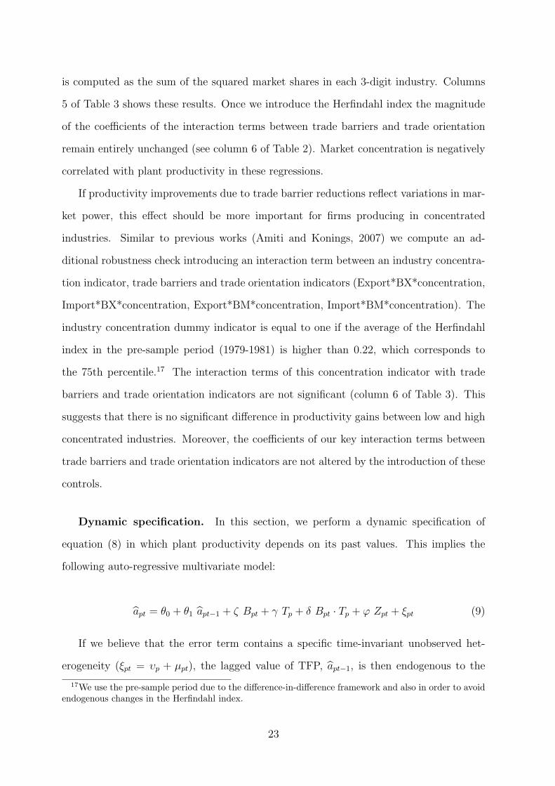
Dynamic specification. In this section, we perform a dynamic specification of

equation (8) in which plant productivity depends on its past values. This implies the

following auto-regressive multivariate model:

apt = θ0 + θ1 apt−1 + ζ Bpt + γ Tp + δ Bpt · Tp + ϕ Zpt + ξpt (9)

If we believe that the error term contains a specific time-invariant unobserved het-

erogeneity (ξpt = υp + µpt), the lagged value of TFP, apt−1, is then endogenous to the

17We use the pre-sample period due to the difference-in-difference framework and also in order to avoidendogenous changes in the Herfindahl index.

23

error term (as it also contains υp). Econometric literature provides well-known strategies

for this dynamic issue. These strategies exploit moment conditions of exogeneity of the

lags of the endogenous dependent variable. Here we use the GMM estimator of Arellano

and Bond (1991). We include OLS and within-group (WG) estimators to identify an

interval within which a consistent estimate of the autoregressive coefficient θ1 should lie

(Bond, 2002). The first column of Table 4 reports the OLS results, the second one the

within-group estimates and finally, column 3 shows the GMM results. As expected, the

coefficient of the auto-regressive term (tfp lp(t-1)) is higher when using OLS than in the

case of within-group regressions. This is a signal of a consistent dynamic specification,

which means that the number of TFP lags on the right-hand side is correct. The set of

instruments used in GMM estimation is composed of deep lags of border effect measures

and TFP. Both set of variables are treated as endogenous. This provides an additional

robustness check on the potential endogeneity issue between border effects and produc-

tivity mentioned in the step 2. The Hansen and Sargan tests validate our instrument

choice. The number of individuals relative to the number of instruments is reassuring as

regards any possible bias in the test when using a large number of instruments (Windmei-

jer, 2005). We focus on GMM and within-group results. Dynamic regressions confirm the

existence of plant productivity improvements after a reduction of export barriers in both

traded industries. The positive sign in the interaction between import barriers and the

import-competing indicator (Import*BM), also resists the dynamic control in GMM re-

gressions. In the case of a within-group estimates this effect fails to be significant, though

the autoregressive coefficient seems clearly downward biased.

[Table 4 about here]

On the contrary, the positive impact of import barrier reductions on plant productivity

in export-oriented industries depends on the method. Within-group estimations confirm

this finding (column 2), while in GMM regressions (column 3) the coefficient of the inter-

action between import barriers and the export-oriented indicator (Export*BM) becomes

positive and significant. If GMM addresses the dynamic panel bias as it is expected, this

24

result means that, once we control for the persistence of plant productivity series, foreign

competition might also dampen domestic sales and plant productivity in export-oriented

industries. Their high productivity trend overwhelms this effect in a static specification

or in the case of a panel data bias in the within-group estimation.

3.3.4 Trade liberalization channels

Increasing returns to scale. One of the novel findings in previous regressions is the

negative impact of import barrier reductions on productivity gains of firms producing in

import-competing industries. This result is robust to alternative measures of productivity

and to controls of market power. In this subsection we provide additional evidence on the

mechanism by which import competition might affect plant productivity.

As previously mentioned, the production function estimates in the first step reveal

IRS in industries classified as import-competing. Hence, one possible explanation is that

foreign competition reduces market shares of all firms and hampers the possibility to

exploit economies of scale in import-competing industries. To illustrate this argument we

provide regressions interacting trade barriers and a dummy indicating whether the plant

operates in an industry under IRS (Increasing).18)

Table 5 presents these results. Firms producing in industries operating under IRS have

a lower productivity level than other firms (column (1)). The interaction term between

import barriers and the indicator of increasing returns to scale is positive and significant

(column (2)). This means that firms producing in industries under IRS suffer from foreign

competition. As expected, the interaction term between export barriers and the indicator

of increasing returns to scale is negative and significant. The reduction of export barriers

increases market potential and enlarges the possibility to exploit scale economies (column

(2)). These results remain robust when we control for market concentration (column (3))

and standard errors corrected for clustering at the plant level (column (4)).

[Table 5 about here]

18The production function estimates show that industries operating under Increasing returns are Textile(32), Paper (34), Chemicals (35) and Machinery (38).

25

The better access to foreign technology. In a developing country like Chile, the

access to new technologies embodied in high-quality imported inputs and capital equip-

ment may have a major role on productivity enhancements. This channel is present in

our data. First, in previous regressions we find that firms producing with imported inputs

have a higher TFP than those that only use domestic inputs. Second, in this subsection

instead of using the import border effect at the 2-digit industry level for each industry, we

only use the one corresponding to Machinery (BK M) as a proxy of import barriers on cap-

ital equipment. The interaction term of this specific import border effect with the trade

orientation dummies captures the extent to which plant productivity reacts to a better

access to foreign capital goods. Table 6 reports the results of these regressions. Relative

to non-traded industries, firms belonging to traded industries enhance their productivity

after a reduction of import barriers on machinery industry. Moreover, productivity gains

are significantly higher for plants in export-oriented industries (Export*BK M) than in

import-competing ones (Import*BK M).

[Table 6 about here]

4 Conclusion

The main contribution of the paper is to construct specific measures of trade barriers

at the industry-level in order to disentangle the impact of the reduction of export and

import barriers on plant productivity. This distinction introduces new results. First, the

reduction of export barriers improves productivity of plants belonging to both traded

industries. As the export costs fall, more firms are able to export increasing their size

and probably benefiting from knowledge spillovers stemming from international markets.

This encouraging result is robust to all robustness checks and specifications. Second, in

all static specifications the reduction of import barriers shows a positive impact on the

evolution of plant productivity in export-oriented industries relative to non-traded. How-

ever, this is not the case for plants belonging to import-competing industries producing

26

with increasing returns to scale. The reduction of import barriers may prevent local firms

to exploit economies of scale since they must share the local market with foreign com-

petitors. Moreover, exporters’ productivity also appears to have a negative reaction to

foreign competition when a dynamic setting is considered.

References

[1] Alvarez, R., and R. Lopez (2005). Exporting and Performance: Evidence from

Chilean Plants. Canadian Journal of Economics 38 (4): 1384-1400.

[2] Amiti, M., and J. Konings (2007). Trade liberalization, intermediate inputs, and

productivity: Evidence from Indonesia. American Economic Review 97 (5): 1611-

1638.

[3] Anderson, J. E., and E. van Wincoop (2003). Gravity with Gravitas : a Solution to

the Border Puzzle. American Economic Review 93 (3): 170-192.

[4] Anderson, J. E., and E. van Wincoop (2004). Trade Costs. Journal of Economic

Literature 42 (1): 691-751.

[5] Arellano, M., and S. Bond (1991). Some Tests of Specification for Panel Data: Monte

Carlo Evidence and an Application to Employment Equations. Review of Economic

Studies 58 (1): 277-297.

[6] Baier, S. L., and Jeffrey H. Bergstrand (2001). The Growth of World Trade: Tariffs,

Transport Costs and Income Similarity. Journal of International Economics 53(1):

1-27.

[7] Bond, S. (2002). Dynamic Panel Data Models: a Guide to Micro Data Methods and

Practice. Portuguese Economic Journal 1: 141-162.

27

[8] Bergoeing, R., P. J. Kehoe, T. J. Kehoe, and R. Soto (2002). Policy-Driven Produc-

tivity in Chile and Mexico in the 1980s and 1990s. American Economic Association

92(2): 16-21.

[9] Bergoeing, R., N. Loayza and A. Repetto (2004). Slow Recoveries. Journal of Devel-

opment Economics 75, 473-506.

[10] Bergoeing, R., A. Hernando and A. Repetto (2006). Market Reforms and Efficiency

Gains in Chile. Working Paper CEA, University of Chile.

[11] Bergoeing, R. , A. Micco and A. Repetto (2005). Dissecting the Chilean Export

Boom. Working Paper CEA, Universidad de Chile.

[12] De Loecker, J. (2007). Do exports generate higher productivity? Evidence from

Slovenia. Journal of International Economics 73(1): 69-98.

[13] Devarajan, S. and D. Rodrik (1989). Trade Liberalization in Developing Countries:

Do Imperfect Competition and Scale Economies Matter?. The American Economic

Review 79(2): 283-287.

[14] Feenstra, R. C. (2003). Advanced International Trade: Theory and Evidence. Prince-

ton University Press.

[15] Fontagne, L., T. Mayer and S. Zignago (2005). Trade in the Triad: How Easy is the

Access to Large Markets?. Canadian Journal of Economics 38(4): 1402-1430.

[16] Harrigan, J. (1996). Openness to Trade in Manufactures in the OECD. Journal of

International Economics 40(1-2): 23-39.

[17] Head, K., and T. Mayer (2000). Non-Europe : The Magnitude and Causes of Market

Fragmentation in Europe. Weltwirschaftliches Archiv 136 (2): 285-314.

[18] Kasahara, H., and J. Rodriguez (2008). Does the Use of Imported Intermediates

Increase Productivity? Plant-Level Evidence. Journal of Development Economics

87: 106-118.

28

[19] Katayama, H. , S. Lu and J. Tybout (2005). Firm-Level Productivity Studies: Illu-

sions and a Solution. NBER Working Paper No. 9617.

[20] Kraay, A. (2002). Exports and Economic Performance: Evidence from a Panel of

Chinese Firms. In M. F. Renard (Ed.). China and its Regions, Economic Growth

and Reform in Chinese Provinces. Cheltenham : Edward Elgar. 278-299.

[21] Levinsohn, J., and A. Petrin (2003). Estimating Production Functions Using Inputs

to Control for Unobservables. Review of Economic Studies 70(2): pp. 317-341.

[22] Liu, L., and J. Tybout (1996). Productivity Growth in Colombia and Chile: Panel-

Based Evidence on the Role of Entry, Exit and Learning. In M. Roberts and J.

Tybout (eds.), Industrial Evolution in Developing Countries. New York : Oxford

University Press.

[23] McCallum, J. (1995). National Borders Matter. American Economic Review 85 (3):

615-23.

[24] Nicita, A., and M. Olarreaga (2001). Trade and Production, 1976-99. Policy Research

Working Paper Series 2701, The World Bank.

[25] Olley, S., and A. Pakes (1996). The Dynamics of Productivity in the Telecommuni-

cation Equipment Industry. Econometrica 64(6): 1263-1298.

[26] Pavcnik, N. (2002). Trade Liberalisation, Exit and Productivity Improvement: Evi-

dence from Chilean Plants. Review of Economic Studies 69: 245-276.

[27] Redding, S., and A. Venables (2004). Economic Geography and International In-

equality. Journal of International Economics 62(1): 53-82.

[28] Rodrik, D. (1988). Closing the Technology gap: Does Trade Liberalization Really

Help?. NBER working paper No. 2654.

29

[29] Schor, A. (2004). Heterogeneous productivity response to tariff reduction: evidence

from Brazilian manufacturing firms. Journal of Development Economics 75(2) :373-

396.

[30] Windmeijer, F. (2005). A Finite Sample Correction for the Variance of Linear Eficient

Two-Step GMM Estimators. Journal of Econometrics 126(1): 25-51.

30

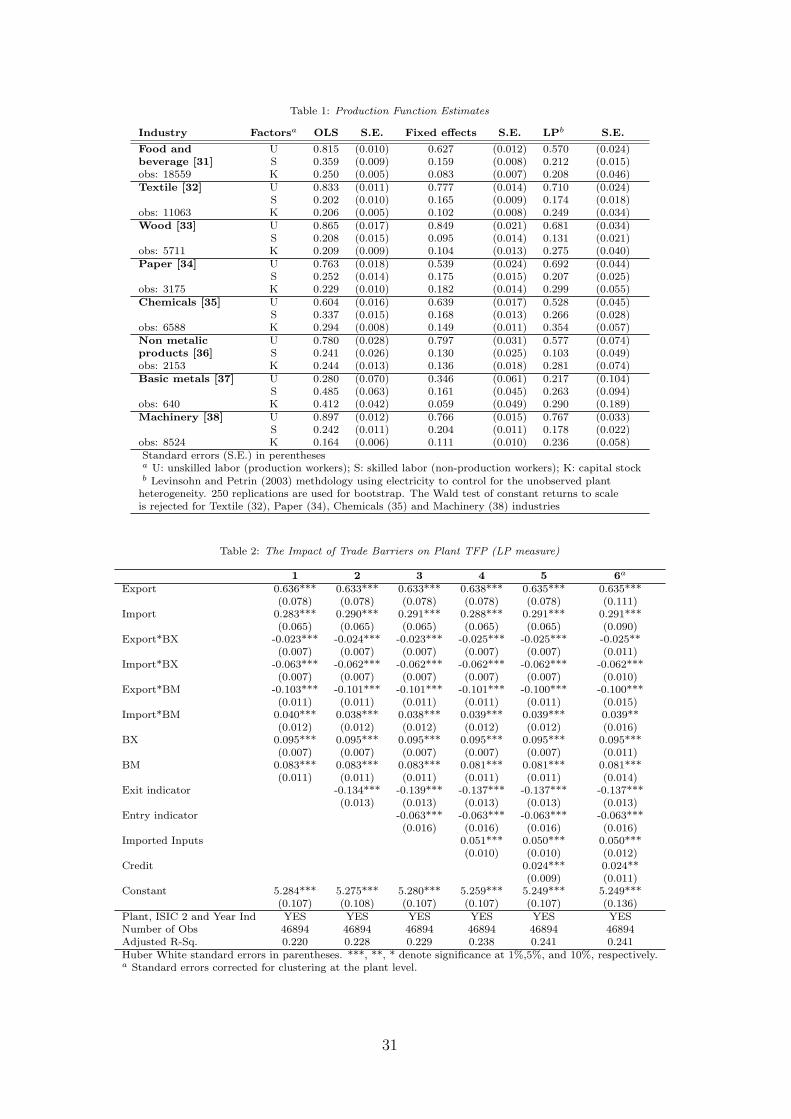
Table 1: Production Function Estimates

Industry Factorsa OLS S.E. Fixed effects S.E. LPb S.E.

Food and U 0.815 (0.010) 0.627 (0.012) 0.570 (0.024)beverage [31] S 0.359 (0.009) 0.159 (0.008) 0.212 (0.015)obs: 18559 K 0.250 (0.005) 0.083 (0.007) 0.208 (0.046)Textile [32] U 0.833 (0.011) 0.777 (0.014) 0.710 (0.024)

S 0.202 (0.010) 0.165 (0.009) 0.174 (0.018)obs: 11063 K 0.206 (0.005) 0.102 (0.008) 0.249 (0.034)Wood [33] U 0.865 (0.017) 0.849 (0.021) 0.681 (0.034)

S 0.208 (0.015) 0.095 (0.014) 0.131 (0.021)obs: 5711 K 0.209 (0.009) 0.104 (0.013) 0.275 (0.040)Paper [34] U 0.763 (0.018) 0.539 (0.024) 0.692 (0.044)

S 0.252 (0.014) 0.175 (0.015) 0.207 (0.025)obs: 3175 K 0.229 (0.010) 0.182 (0.014) 0.299 (0.055)Chemicals [35] U 0.604 (0.016) 0.639 (0.017) 0.528 (0.045)

S 0.337 (0.015) 0.168 (0.013) 0.266 (0.028)obs: 6588 K 0.294 (0.008) 0.149 (0.011) 0.354 (0.057)Non metalic U 0.780 (0.028) 0.797 (0.031) 0.577 (0.074)products [36] S 0.241 (0.026) 0.130 (0.025) 0.103 (0.049)obs: 2153 K 0.244 (0.013) 0.136 (0.018) 0.281 (0.074)Basic metals [37] U 0.280 (0.070) 0.346 (0.061) 0.217 (0.104)

S 0.485 (0.063) 0.161 (0.045) 0.263 (0.094)obs: 640 K 0.412 (0.042) 0.059 (0.049) 0.290 (0.189)Machinery [38] U 0.897 (0.012) 0.766 (0.015) 0.767 (0.033)

S 0.242 (0.011) 0.204 (0.011) 0.178 (0.022)obs: 8524 K 0.164 (0.006) 0.111 (0.010) 0.236 (0.058)Standard errors (S.E.) in perenthesesa U: unskilled labor (production workers); S: skilled labor (non-production workers); K: capital stockb Levinsohn and Petrin (2003) methdology using electricity to control for the unobserved plant

heterogeneity. 250 replications are used for bootstrap. The Wald test of constant returns to scaleis rejected for Textile (32), Paper (34), Chemicals (35) and Machinery (38) industries

Table 2: The Impact of Trade Barriers on Plant TFP (LP measure)

1 2 3 4 5 6a

Export 0.636*** 0.633*** 0.633*** 0.638*** 0.635*** 0.635***(0.078) (0.078) (0.078) (0.078) (0.078) (0.111)

Import 0.283*** 0.290*** 0.291*** 0.288*** 0.291*** 0.291***(0.065) (0.065) (0.065) (0.065) (0.065) (0.090)

Export*BX -0.023*** -0.024*** -0.023*** -0.025*** -0.025*** -0.025**(0.007) (0.007) (0.007) (0.007) (0.007) (0.011)

Import*BX -0.063*** -0.062*** -0.062*** -0.062*** -0.062*** -0.062***(0.007) (0.007) (0.007) (0.007) (0.007) (0.010)

Export*BM -0.103*** -0.101*** -0.101*** -0.101*** -0.100*** -0.100***(0.011) (0.011) (0.011) (0.011) (0.011) (0.015)

Import*BM 0.040*** 0.038*** 0.038*** 0.039*** 0.039*** 0.039**(0.012) (0.012) (0.012) (0.012) (0.012) (0.016)

BX 0.095*** 0.095*** 0.095*** 0.095*** 0.095*** 0.095***(0.007) (0.007) (0.007) (0.007) (0.007) (0.011)

BM 0.083*** 0.083*** 0.083*** 0.081*** 0.081*** 0.081***(0.011) (0.011) (0.011) (0.011) (0.011) (0.014)

Exit indicator -0.134*** -0.139*** -0.137*** -0.137*** -0.137***(0.013) (0.013) (0.013) (0.013) (0.013)

Entry indicator -0.063*** -0.063*** -0.063*** -0.063***(0.016) (0.016) (0.016) (0.016)

Imported Inputs 0.051*** 0.050*** 0.050***(0.010) (0.010) (0.012)

Credit 0.024*** 0.024**(0.009) (0.011)

Constant 5.284*** 5.275*** 5.280*** 5.259*** 5.249*** 5.249***(0.107) (0.108) (0.107) (0.107) (0.107) (0.136)

Plant, ISIC 2 and Year Ind YES YES YES YES YES YESNumber of Obs 46894 46894 46894 46894 46894 46894Adjusted R-Sq. 0.220 0.228 0.229 0.238 0.241 0.241Huber White standard errors in parentheses. ***, **, * denote significance at 1%,5%, and 10%, respectively.a Standard errors corrected for clustering at the plant level.

31

Table 3: Alternative Measures of Productivity and Controls for Mark-up

TFP FE TFP FEa Labor pr. Labor pr.b TFP LP TFP LPc

Export 0.524*** 0.520*** 0.489*** 0.540*** 0.617*** 0.798***(0.074) (0.105) (0.063) (0.098) (0.111) (0.162)

Import 0.227*** 0.232*** 0.296*** 0.291*** 0.304*** 0.358***(0.062) (0.082) (0.058) (0.083) (0.092) (0.097)

Export*BX -0.019*** -0.020* -0.020*** -0.022** -0.024** -0.024**(0.007) (0.010) (0.006) (0.010) (0.011) (0.011)

Import*BX -0.059*** -0.059*** -0.067*** -0.066*** -0.062*** -0.064***(0.007) (0.010) (0.006) (0.009) (0.010) (0.010)

Export*BM -0.090*** -0.090*** -0.083*** -0.090*** -0.099*** -0.104***(0.011) (0.015) (0.010) (0.014) (0.015) (0.015)

Import*BM 0.051*** 0.050*** 0.048*** 0.051*** 0.039** 0.040**(0.012) (0.016) (0.011) (0.015) (0.016) (0.017)

BX 0.092*** 0.092*** 0.078*** 0.081*** 0.095*** 0.095***(0.007) (0.010) (0.006) (0.010) (0.011) (0.011)

BM 0.062*** 0.063*** 0.069*** 0.075*** 0.080*** 0.086***(0.010) (0.014) (0.010) (0.014) (0.014) (0.015)

Exit indicator -0.146*** -0.145*** -0.146*** -0.150*** -0.136*** -0.137***(0.013) (0.013) (0.010) (0.013) (0.013) (0.013)

Entry indicator -0.067*** -0.066*** -0.027*** -0.049*** -0.062*** -0.063***(0.015) (0.016) (0.010) (0.015) (0.016) (0.016)

Imported Inputs 0.064*** 0.063*** 0.065*** 0.058*** 0.050*** 0.050***(0.010) (0.012) (0.009) (0.012) (0.012) (0.012)

Credit 0.032*** 0.030*** 0.025** 0.024**(0.010) (0.010) (0.011) (0.011)

Capital Intensity 0.081***(0.007)

Herfindahl -0.218*(0.129)

Export*BX*Concentration 0.047(0.047)

Import*BX*Concentration 0.044(0.042)

Export*BM*Concentration -0.058(0.059)

Import*BM*Concentration -0.094(0.064)

Concentration -0.178(0.192)

Constant 6.660*** 6.647*** 7.152*** 6.567*** 5.253*** 5.151***(0.106) (0.130) (0.090) (0.137) (0.135) (0.140)

Number of Obs 46894 46894 65068 49001 46894 46894Adjusted R-Sq. 0.207 0.214 0.106 0.235 0.241 0.234Plant, ISIC 2 and Year Ind YES YES YES YES YES YESNumber of Obs 46894 46894 65068 49001 46894 46894Adjusted R-Sq. 0.207 0.214 0.106 0.235 0.241 0.235Huber White standard errors in parentheses. ***, **, * denote significance at 1%,5%, and 10%, respectively.Fixed effect TFP (TFP FE) and labor productivity (Labor pr.) are considered as alternative measuresof the LP TFP. The last two columns address potential markup bias concerns by adding the Concentrationdummy, which indicates if the average Herfindahl index in the pre-sample period is in the 75th percentile.a,b,c Standard errors corrected for clustering at the plant level.

32

Table 4: Dynamic specification

1 2a 3b

TFP(t-1) 0.822*** 0.482*** 0.741***(0.005) (0.009) (0.091)

Export 0.233*** 0.400*** -1.853(0.044) (0.101) (2.221)

Import 0.021 0.137* -1.061(0.037) (0.081) (1.731)

Export*BX -0.016*** -0.020** -0.233***(0.006) (0.008) (0.067)

Import*BX -0.016*** -0.034*** -0.343***(0.005) (0.008) (0.110)

Export*BM -0.030*** -0.052*** 0.358***(0.008) (0.012) (0.098)

Import*BM 0.015* 0.019 0.515***(0.008) (0.013) (0.154)

BX 0.043*** 0.066*** 0.220**(0.006) ((0.008) (0.086)

BM -0.009 0.030*** -0.346***(0.008) (0.011) (0.113)

Herfindahl -0.008 0.099 0.593(0.065) (0.109) (0.811)

Exit indicator -0.148*** -0.115*** -0.262***(0.012) (0.014) (0.039)

Entry indicator 0.000 0.000(0.000) (0.000)

Credit 0.041*** 0.013 0.604**(0.006) (0.009) (0.266)

Imported Inputs 0.081*** 0.035*** 0.077(0.006) (0.010) (0.137)

Constant 0.722*** 2.672***(0.049) (0.134)

Plant, ISIC 2 and Year Ind YES YES YESNumber of Obs 35117 35117 31853Adjusted R-Sq. 0.757 0.287Sargan p 0.160Hansen p 0.248AR(2)p 0.002c

AR(3)p 0.810instruments 85individuals 5392 4911Huber White standard errors in parentheses.***, **, * denote significance at 1%,5%, and 10%, respectively.a Standard errors corrected for clustering at the plant level.b The set of instruments is composed of lagged values of bordereffect and plant TFP. Both are treated as endogenous vairables. Asusual, we use industry and year indicators as exogenous instruments.Orthogonal transformations are used to maximize sample size.c Since the Arellano-Bond test of autocorrelation reveals that thedisturbance might be in itself auto-correlated of order-1, but notfurther, we take lags between t - 4 and t -6.

33

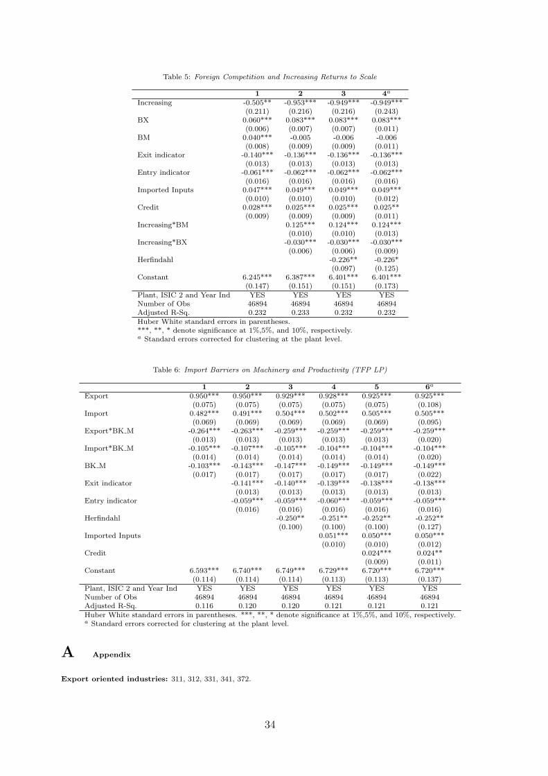
Table 5: Foreign Competition and Increasing Returns to Scale

1 2 3 4a

Increasing -0.505** -0.953*** -0.949*** -0.949***(0.211) (0.216) (0.216) (0.243)

BX 0.060*** 0.083*** 0.083*** 0.083***(0.006) (0.007) (0.007) (0.011)

BM 0.040*** -0.005 -0.006 -0.006(0.008) (0.009) (0.009) (0.011)

Exit indicator -0.140*** -0.136*** -0.136*** -0.136***(0.013) (0.013) (0.013) (0.013)

Entry indicator -0.061*** -0.062*** -0.062*** -0.062***(0.016) (0.016) (0.016) (0.016)

Imported Inputs 0.047*** 0.049*** 0.049*** 0.049***(0.010) (0.010) (0.010) (0.012)

Credit 0.028*** 0.025*** 0.025*** 0.025**(0.009) (0.009) (0.009) (0.011)

Increasing*BM 0.125*** 0.124*** 0.124***(0.010) (0.010) (0.013)

Increasing*BX -0.030*** -0.030*** -0.030***(0.006) (0.006) (0.009)

Herfindahl -0.226** -0.226*(0.097) (0.125)

Constant 6.245*** 6.387*** 6.401*** 6.401***(0.147) (0.151) (0.151) (0.173)

Plant, ISIC 2 and Year Ind YES YES YES YESNumber of Obs 46894 46894 46894 46894Adjusted R-Sq. 0.232 0.233 0.232 0.232Huber White standard errors in parentheses.***, **, * denote significance at 1%,5%, and 10%, respectively.a Standard errors corrected for clustering at the plant level.

Table 6: Import Barriers on Machinery and Productivity (TFP LP)

1 2 3 4 5 6a

Export 0.950*** 0.950*** 0.929*** 0.928*** 0.925*** 0.925***(0.075) (0.075) (0.075) (0.075) (0.075) (0.108)

Import 0.482*** 0.491*** 0.504*** 0.502*** 0.505*** 0.505***(0.069) (0.069) (0.069) (0.069) (0.069) (0.095)

Export*BK M -0.264*** -0.263*** -0.259*** -0.259*** -0.259*** -0.259***(0.013) (0.013) (0.013) (0.013) (0.013) (0.020)

Import*BK M -0.105*** -0.107*** -0.105*** -0.104*** -0.104*** -0.104***(0.014) (0.014) (0.014) (0.014) (0.014) (0.020)

BK M -0.103*** -0.143*** -0.147*** -0.149*** -0.149*** -0.149***(0.017) (0.017) (0.017) (0.017) (0.017) (0.022)

Exit indicator -0.141*** -0.140*** -0.139*** -0.138*** -0.138***(0.013) (0.013) (0.013) (0.013) (0.013)

Entry indicator -0.059*** -0.059*** -0.060*** -0.059*** -0.059***(0.016) (0.016) (0.016) (0.016) (0.016)

Herfindahl -0.250** -0.251** -0.252** -0.252**(0.100) (0.100) (0.100) (0.127)

Imported Inputs 0.051*** 0.050*** 0.050***(0.010) (0.010) (0.012)

Credit 0.024*** 0.024**(0.009) (0.011)

Constant 6.593*** 6.740*** 6.749*** 6.729*** 6.720*** 6.720***(0.114) (0.114) (0.114) (0.113) (0.113) (0.137)

Plant, ISIC 2 and Year Ind YES YES YES YES YES YESNumber of Obs 46894 46894 46894 46894 46894 46894Adjusted R-Sq. 0.116 0.120 0.120 0.121 0.121 0.121Huber White standard errors in parentheses. ***, **, * denote significance at 1%,5%, and 10%, respectively.a Standard errors corrected for clustering at the plant level.

A Appendix

Export oriented industries: 311, 312, 331, 341, 372.

34

Import competing industries: 321, 322, 351, 354, 355, 361, 362, 381, 382, 383, 384, 385, 390.

Non traded industries: 313, 323, 324, 332, 342, 352, 353, 356, 369, 371.

Table 7: Variables description

Variable DataExport Border Effect BX Export barriers at 2 digit industry level estimated

by a gravity model in step 2.Import Border Effect BM Import barriers at 2 digit industry level estimated

by a gravity model in step 2.Export oriented sector Export Dummy variable equal to one if the firm belongs to a

3 digit industry with more than 15% of exports over outputImport competing sector Import Dummy variable equal to one if the firm belongs to a

3 digit industry with more than 15% of import over outputMarket concentration Herfindahl Herfindahl index of market concentration

at 3 digit industry levelPre-sample Concentration Concentration Dummy variable equal if the average Herfindahl index

in the pre-sample period is in the 75th percentileImported Inputs Imported Inputs Dummy variable equal to one if the plant reports

having used imported inputsCredit Indicator Credit Dummy variable equal to one if the plant reports

having paid a loan tax in year ”‘t”’

Table 8: Summary Statistics by Industry (2-digit ISIC Rev-2)

Labor pr. ∆ Labor pr. S/L K/L Exports shareFood (31) 5108 0.10 0.13 3420 0.09

(10204) (0.66) (0.11) (10709) (0.2)Textile (32) 3828 0.07 0.13 2198 0.02

(3770) (0.5) (0.10) (8676) (0.09)Wood (33) 4099 0.11 0.11 2192 0.07

(6428) (0.93) (0.10) (4143) (0.18)Paper (34) 7119 0.02 0.17 4775 0.03

(9492) (0.42) (0.15) (14877) (0.12)Chemicals (35) 10832 0.07 0.16 4793 0.04

(23366) (0.57) (0.11) (10573) (0.13)Non metallic (36) 8130 0.09 0.13 5356 0.01

(14480) (0.59) (0.10) (16133) (0.06)Basic metals (37) 34409 0.13 0.19 7826 0.18

(93787) (0.71) (0.14) (12033) (0.31)Machinery (38) 5375 0.10 0.16 3122 0.02

(5987) (0.68) (0.13) (6519) (0.07)

Mean of variables reported; standar deviation in parenthesesLabor pr.: labor productivity, ∆ Labor pr.: Labor productivity growth, S/L: skill intensity,K/L: capital intensity

0,94

0,96

0,98

1

1,02

1,04

1,06

1,08

1,1

1979 1981 1983 1985 1987 1989 1991 1993 1995 1997 1999

tfp_lp tfp_fe tfp_ols lnproductivity

35

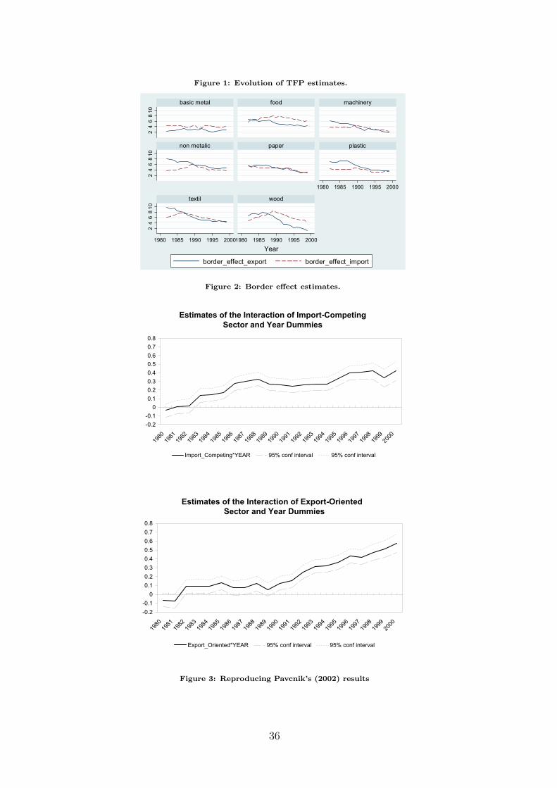
Figure 1: Evolution of TFP estimates.

24

68

10

24

68

10

24

68

10

1980 1985 1990 1995 2000

1980 1985 1990 1995 20001980 1985 1990 1995 2000

basic metal food machinery

non metalic paper plastic

textil wood

border_effect_export border_effect_import

Year

Figure 2: Border effect estimates.

Estimates of the Interaction of Import-Competing

Sector and Year Dummies

-0.2

-0.1

0

0.1

0.2

0.3

0.4

0.5

0.6

0.7

0.8

1980

1981

1982

1983

1984

1985

1986

1987

1988

1989

1990

1991

1992

1993

1994

1995

1996

1997

1998

1999

2000

Import_Competing*YEAR 95% conf interval 95% conf interval

Estimates of the Interaction of Export-Oriented

Sector and Year Dummies

-0.2

-0.1

0

0.1

0.2

0.3

0.4

0.5

0.6

0.7

0.8

1980

1981

1982

1983

1984

1985

1986

1987

1988

1989

1990

1991

1992

1993

1994

1995

1996

1997

1998

1999

2000

Export_Oriented*YEAR 95% conf interval 95% conf interval

Figure 3: Reproducing Pavcnik’s (2002) results

36

B Technical appendix

We classify industries by trade orientation at the 3-digit industry level similar to Pavcnik(2002)(Table 1.B). Plants are classified as export-oriented if they belong to a 3-digit in-dustry which has more than 15% of exports over total production (Export-Output ratio)and as import-competing if the industry has more than 15% of imports over total produc-tion (Import-Output ratio). The rest are considered as non-traded. There are only twoindustries (351 and 384) that matched up to both categories. Nevertheless, the industry351 (384) presents an export-output ratio of 0.82 (0.21) and an import-output ratio of 1.32(2.01). Therefore these industries were classified as import competing in the paper. Ourresults remain unchanged if we consider a fourth category of export-import competing(Export-Import) for industries 351 and 384. Table 2.B and 3.B report the results withthis classification (Export-oriented, Import-competing and Export-Import). The interac-tion terms between trade barriers and trade orientation status (Export*BX,Import*BX,Export*BM and Import*BM) are very similar to the previous results with the originalclassification that considers industries 351 and 384 as import-competing (Table 2 and 3in main text of the paper).

Table 1.B.: Trade orientation classification

Import competing Export-Output Import-Outputindustries ratio ratio

321 0.006 0.271322 0.004 0.174354 0.019 0.262355 0.040 0.296361 0.092 0.716362 0.017 0.318381 0.097 0.255382 0.053 2.141383 0.036 1.649385 0.089 7.381

Import competing or Export-Import

351 0.824 1.326384 0.210 2.010

Export oriented

311 0.212 0.104312 0.174 0.078331 0.254 0.019341 0.418 0.096372 0.733 0.012

Non traded

313 0.046 0.045323 0.008 0.135324 0.004 0.097332 0.016 0.089342 0.023 0.062352 0.002 0.113353 0.029 0.114356 0.002 0.102

Note: All reported figures are averages over 1980-1986. Source: Pavcnik (2002)

37

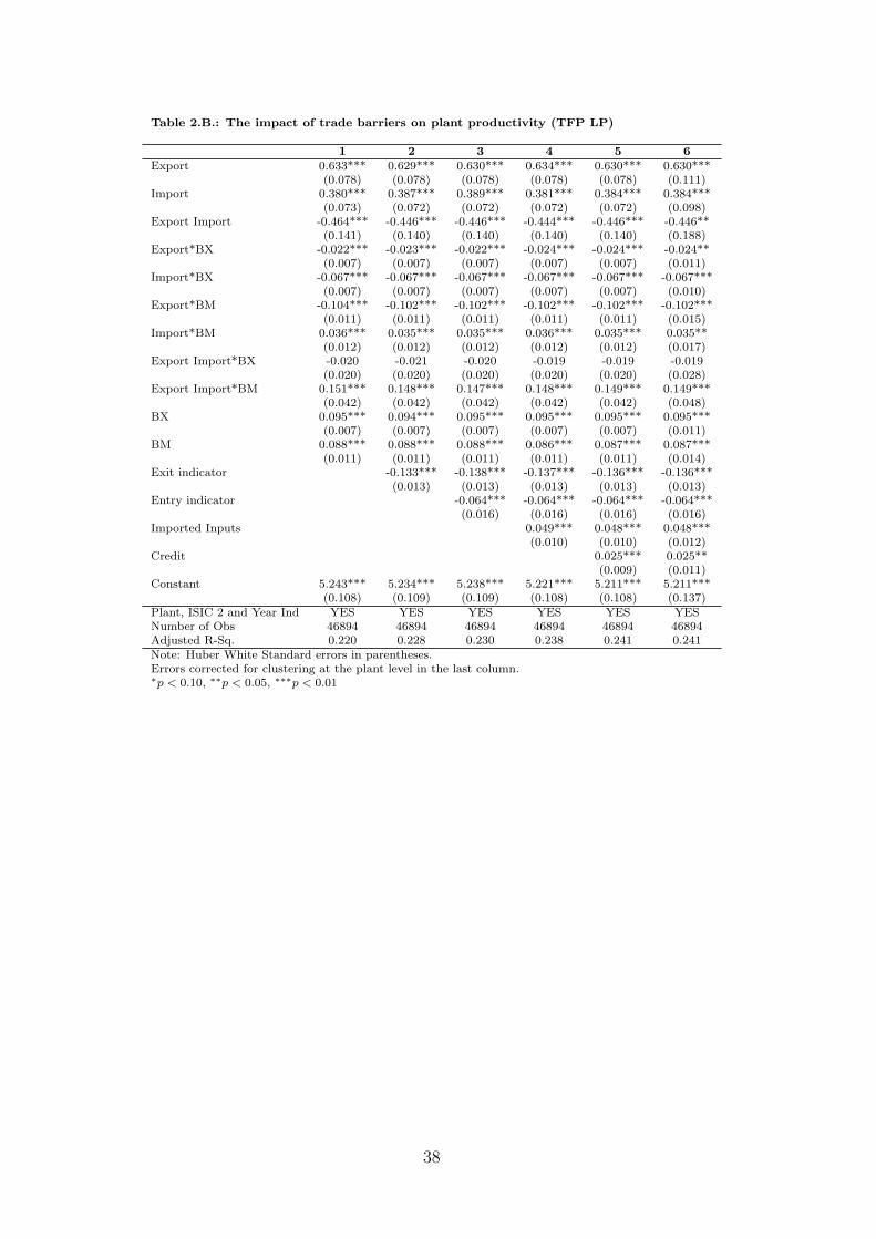
Table 2.B.: The impact of trade barriers on plant productivity (TFP LP)

1 2 3 4 5 6Export 0.633*** 0.629*** 0.630*** 0.634*** 0.630*** 0.630***

(0.078) (0.078) (0.078) (0.078) (0.078) (0.111)Import 0.380*** 0.387*** 0.389*** 0.381*** 0.384*** 0.384***

(0.073) (0.072) (0.072) (0.072) (0.072) (0.098)Export Import -0.464*** -0.446*** -0.446*** -0.444*** -0.446*** -0.446**

(0.141) (0.140) (0.140) (0.140) (0.140) (0.188)Export*BX -0.022*** -0.023*** -0.022*** -0.024*** -0.024*** -0.024**

(0.007) (0.007) (0.007) (0.007) (0.007) (0.011)Import*BX -0.067*** -0.067*** -0.067*** -0.067*** -0.067*** -0.067***

(0.007) (0.007) (0.007) (0.007) (0.007) (0.010)Export*BM -0.104*** -0.102*** -0.102*** -0.102*** -0.102*** -0.102***

(0.011) (0.011) (0.011) (0.011) (0.011) (0.015)Import*BM 0.036*** 0.035*** 0.035*** 0.036*** 0.035*** 0.035**

(0.012) (0.012) (0.012) (0.012) (0.012) (0.017)Export Import*BX -0.020 -0.021 -0.020 -0.019 -0.019 -0.019

(0.020) (0.020) (0.020) (0.020) (0.020) (0.028)Export Import*BM 0.151*** 0.148*** 0.147*** 0.148*** 0.149*** 0.149***

(0.042) (0.042) (0.042) (0.042) (0.042) (0.048)BX 0.095*** 0.094*** 0.095*** 0.095*** 0.095*** 0.095***

(0.007) (0.007) (0.007) (0.007) (0.007) (0.011)BM 0.088*** 0.088*** 0.088*** 0.086*** 0.087*** 0.087***

(0.011) (0.011) (0.011) (0.011) (0.011) (0.014)Exit indicator -0.133*** -0.138*** -0.137*** -0.136*** -0.136***

(0.013) (0.013) (0.013) (0.013) (0.013)Entry indicator -0.064*** -0.064*** -0.064*** -0.064***

(0.016) (0.016) (0.016) (0.016)Imported Inputs 0.049*** 0.048*** 0.048***

(0.010) (0.010) (0.012)Credit 0.025*** 0.025**

(0.009) (0.011)Constant 5.243*** 5.234*** 5.238*** 5.221*** 5.211*** 5.211***

(0.108) (0.109) (0.109) (0.108) (0.108) (0.137)Plant, ISIC 2 and Year Ind YES YES YES YES YES YESNumber of Obs 46894 46894 46894 46894 46894 46894Adjusted R-Sq. 0.220 0.228 0.230 0.238 0.241 0.241Note: Huber White Standard errors in parentheses.Errors corrected for clustering at the plant level in the last column.∗p < 0.10, ∗∗p < 0.05, ∗∗∗p < 0.01

38

Table 3.B.: Robutness checks

TFP FE TFP FE VA L VA L TFP LP TFP LPExport 0.523*** 0.518*** 0.493*** 0.538*** 0.616*** 0.794***

(0.074) (0.105) (0.064) (0.098) (0.111) (0.163)Import 0.330*** 0.335*** 0.401*** 0.384*** 0.392*** 0.472***

(0.069) (0.091) (0.062) (0.091) (0.098) (0.109)Export Import -0.400*** -0.403** -0.160 -0.308* -0.427** -0.364*

(0.134) (0.173) (0.121) (0.171) (0.189) (0.193)Export*BX -0.019*** -0.019* -0.019*** -0.021** -0.024** -0.023**

(0.007) (0.010) (0.006) (0.010) (0.011) (0.011)Import*BX -0.062*** -0.061*** -0.067*** -0.068*** -0.066*** -0.068***

(0.007) (0.010) (0.006) (0.010) (0.010) (0.010)Export*BM -0.091*** -0.091*** -0.084*** -0.091*** -0.100*** -0.106***

(0.011) (0.015) (0.010) (0.014) (0.015) (0.015)Import*BM 0.046*** 0.045*** 0.042*** 0.046*** 0.036** 0.037**

(0.012) (0.016) (0.011) (0.016) (0.017) (0.017)Export Import*BX -0.038* -0.038 -0.071*** -0.045* -0.019 -0.021

(0.020) (0.026) (0.018) (0.025) (0.028) (0.028)Export Import*BM 0.158*** 0.160*** 0.141*** 0.153*** 0.148*** 0.145***

(0.040) (0.046) (0.036) (0.047) (0.048) (0.048)BX 0.091*** 0.091*** 0.077*** 0.081*** 0.095*** 0.096***

(0.007) (0.010) (0.006) (0.010) (0.011) (0.011)BM 0.066*** 0.067*** 0.073*** 0.079*** 0.085*** 0.091***

(0.010) (0.014) (0.010) (0.014) (0.014) (0.015)Exit indicator -0.146*** -0.145*** -0.146*** -0.150*** -0.136*** -0.136***

(0.013) (0.013) (0.010) (0.013) (0.013) (0.013)Entry indicator -0.068*** -0.067*** -0.028*** -0.050*** -0.064*** -0.064***

(0.015) (0.016) (0.010) (0.015) (0.016) (0.016)Imported Inputs 0.063*** 0.061*** 0.062*** 0.056*** 0.048*** 0.048***

(0.010) (0.012) (0.009) (0.012) (0.012) (0.012)Credit 0.033*** 0.030*** 0.025** 0.025**

(0.010) (0.010) (0.011) (0.011)lnK L 0.081***

(0.007)Herfindahl -0.178

(0.128)Export*BX*concentration 0.045

(0.047)Import*BX*concentration 0.046

(0.042)Export*BM*concentration -0.052

(0.060)Import*BM*concentration -0.103

(0.064)Export Import*BX*concentration 0.000

(0.000)Export Import*BX*concentration 0.000

(0.000)concentration -0.195

(0.194)Constant 6.614*** 6.601*** 7.102*** 6.524*** 5.216*** 5.095***

(0.107) (0.132) (0.091) (0.138) (0.137) (0.144)Number of Obs 46894 46894 65068 49001 46894 46894Adjusted R-Sq. 0.206 0.213 0.102 0.229 0.241 0.234Note: Huber White Standard errors in parentheses.Errors corrected for clustering at the plant level in column 2, 4, 5 and 6.∗p < 0.10, ∗∗p < 0.05, ∗∗∗p < 0.01

39