Trade Costs and Mark-Ups in Maritime Shipping
65
Trade Costs and Mark-Ups in Maritime Shipping Manuel I. Jimenez * April 19, 2021 Abstract Transportation costs represent about 15% of global import value. Non-competitive pricing behavior is the maritime shipping market is also widely believed to raise the cost of freight. Using U.S. import data, this paper estimates the effects of this presumably non-competitive behavior on (1) total freight costs, (2) international trade flows, and (3) economic welfare. It also evaluates whether such behavior disproportionately affects shipments from developing and/or countries distant from the U.S. To this aim, short-run pass-through rates of cost to freight rates are estimated and used to calculate the freight mark-ups charged on U.S. imports shipped by sea during 2002-2007, 2008-2012 and 2013-2017. The estimates show that freight mark-ups account for approximately one-third of total freight charges in U.S. imports, equiva- lent to an ad valorem tariff of 1.4-2.6 percent. U.S. imports would be 4.2 to 11.6 percent higher if these mark-ups were eliminated. The cost of these mark-ups in terms of economic welfare for U.S. consumers represents a reduction of approximately 0.1-0.2 percent of their real income. Goods imported from developing countries or from countries at greater distances to the U.S. have larger tariff equivalent mark-ups. Keywords: Maritime Shipping Mark-Ups, Trade Costs, Welfare JEL Codes: D43, F14, L11, R41 * Department of Agricultural Economics, Purdue University, 403 W State Street, Krannert Building Rm 610, West Lafayette IN, 47907; e-mail: [email protected]. This research was financed by USDA NIFA grant #2020-67023- 30963. I thank Russell Hillberry, David Hummels, Anson Soderbery, Farid Farrokhi, Joseph Balagtas, Dominique van der Mensbrugghe, and Dave Donaldson for helpful advice and comments. All errors are my own.
Transcript of Trade Costs and Mark-Ups in Maritime Shipping

Trade Costs and Mark-Ups in Maritime Shipping
Manuel I. Jimenez∗
April 19, 2021
Abstract
Transportation costs represent about 15% of global import value. Non-competitive pricingbehavior is the maritime shipping market is also widely believed to raise the cost of freight.Using U.S. import data, this paper estimates the effects of this presumably non-competitivebehavior on (1) total freight costs, (2) international trade flows, and (3) economic welfare. Italso evaluates whether such behavior disproportionately affects shipments from developingand/or countries distant from the U.S. To this aim, short-run pass-through rates of cost tofreight rates are estimated and used to calculate the freight mark-ups charged on U.S. importsshipped by sea during 2002-2007, 2008-2012 and 2013-2017. The estimates show that freightmark-ups account for approximately one-third of total freight charges in U.S. imports, equiva-lent to an ad valorem tariff of 1.4-2.6 percent. U.S. imports would be 4.2 to 11.6 percent higher ifthese mark-ups were eliminated. The cost of these mark-ups in terms of economic welfare forU.S. consumers represents a reduction of approximately 0.1-0.2 percent of their real income.Goods imported from developing countries or from countries at greater distances to the U.S.have larger tariff equivalent mark-ups.
Keywords: Maritime Shipping Mark-Ups, Trade Costs, Welfare
JEL Codes: D43, F14, L11, R41
∗Department of Agricultural Economics, Purdue University, 403 W State Street, Krannert Building Rm 610, WestLafayette IN, 47907; e-mail: [email protected]. This research was financed by USDA NIFA grant #2020-67023-30963. I thank Russell Hillberry, David Hummels, Anson Soderbery, Farid Farrokhi, Joseph Balagtas, Dominiquevan der Mensbrugghe, and Dave Donaldson for helpful advice and comments. All errors are my own.

1 Introduction
Maritime shipping is the most important mode of transportation used in international trade.
About 70% to 80% of international trade flows (in value) move by sea (UNCTAD, 2017). Inter-
national trade is thus highly dependent on an industry in which suppliers are widely believed
to exert market power. Empirical research finds that two main reasons underlie carriers’ mar-
ket power in international shipping. First, excessive shipping capacity supplied in the market
by larger carriers companies, along with the significant economies of scope they exploit, lead to
the concentration of the market in fewer companies (Hummels et al., 2009).1 Second, the lack
of anti-trust enforcement policies allows carriers to make price-fixing agreements (Fink, 2002).2
Although previous studies find evidence that market power exists in the maritime shipping in-
dustry, the literature still lacks absolute measures of the mark-ups that carriers charge.3 Such
estimates would allow: (1) a decomposition of the freight cost into shipping costs and shipping
mark-ups; (2) a comparison with other trade costs, including tariffs; (3) a quantification of the ef-
fects of market power in the maritime shipping industry on trade flows and economic welfare; and
(4) an evaluation of whether non-competitive behavior in the maritime shipping industry dispro-
portionately affects developing and/or countries that are geographically distant from destination
markets.
Atkin and Donaldson (2015) developed an innovative methodology for estimating intermediaries’
trade costs in a market with variable mark-ups. Using theoretical insights from the Industrial Or-
ganization literature, they show that the short-run pass-through rate of costs to prices is a sufficient
statistic for quantifying the response of mark-ups to trade cost changes (Weyl and Fabinger, 2013).
Furthermore, the short-run pass-through rate in the two-stage method proposed theoretical iden-
tification of firms’ marginal costs and mark-ups. I apply thus this methodology in this paper to
the maritime shipping industry, using U.S. import data for the period 2002-2017. The objective is
to quantify the effect of non-competitive pricing behavior on the cost of freight.
The main questions that this paper answers are: How much higher are freight rates than they
would be without non-competitive pricing behavior? What is the effect of shipping mark-ups on1In the liner shipping market, for instance, half of the routes are attended by at most three carriers, and in almost
three-quarters of them by five shipping carriers (UNCTAD, 2017).2Many countries, arguing economic and national security interests, have also domestically kept in place Cargo
Reservation Schemes (e.g. The Jones Act in the USA) to protect this industry (Fink, 2002). Consequently, competi-tion is widely believed is limited in their shipping markets.
3See Fink (2002) and Hummels et al. (2009).
1

trade flows? What are the welfare costs of these mark-ups? To the extent it provides an answer to
these questions, this paper also answers further questions, such as: How large are shipping carri-
ers’ mark-ups relative to tariffs? Do market conditions in shipping routes to smaller destination
ports allow carriers to charge larger mark-ups? Do developing pay higher shipping mark-ups?
Are mark-ups larger on longer routes?
This paper is related to three strands of the literature. First, it contributes to the debate over the
presence of market power in the maritime shipping industry.4 The most closely related paper is
Hummels et al. (2009). However, this paper differs from that study by (1) estimating absolute,
rather than relative, measures of maritime shipping mark-ups; (2) calculating their implied ef-
fect on trade flows and economic welfare; and (3) evaluating whether developing and/or distant
countries pay higher shipping mark-ups.5
Second, this paper contributes to the literature on (1) the underlying mechanisms that determine
freight costs, and (2) the effects of freight costs on international trade. Academic research on this
topic attempts to understand and quantify sources of freight costs.6 Other studies estimate the
impact of freight charges on countries’ export performance.7 Other works document the evolution
of freight costs over time, and examine the underlying market conditions that determine these
costs.8 This paper contributes to this literature by (1) decomposing total shipping freight rates into
marginal cost and mark-up components, and (2) providing quantitative estimates of the degree to
which positive freight mark-ups reduce international trade flows and welfare.
Finally, this paper also expands the growing literature that operationalizes the short-run pass-
through rates of cost to prices for identifying the presence of market power. The seminal paper
in this strand of the literature is Atkin and Donaldson (2015). As noted, that study shows that
the short-run pass-through rate is a sufficient statistic for quantifying the response of mark-ups to
4See e.g. Heaver (1973), Bryan (1974), Devanney III et al. (1975), Davies (1986), Clyde and Reitzes (1998) andFink (2002) and Hummels et al. (2009).
5The underlying CES preference structure assumed by Hummels et al. (2009) does not allow that study to calculatethe shipping mark-ups. Recently, Asturias (2019) estimates these mark-ups, aiming to model the importance of thetransportation sector for trade. However, Asturias uses data for containerized shipping services for the year 2014,and exploits the cross-section variation in that year. In this paper, I use panel data and exploit the time variation.
6See e.g. Limao and Venables (2001), Micco and Perez (2001), Sanchez et al. (2003), Clark et al. (2004),Wilmsmeier et al. (2006), Martınez-Zarzoso et al. (2008) and Wilmsmeier and Hoffmann (2008).
7See e.g. Amjadi and Yeats (1995), Radelet and Sachs (1998), Hummels and Skiba (2004) and Korinek andSourdin (2009).
8See e.g. Hummels and Skiba (2002), Hummels (2007), Hoffmann and Kumar (2013), Brancaccio et al. (2020),Wong (2017), Ardelean and Lugovskyy (2018) and Asturias (2019).
2

trade cost changes. Other recent studies have also successfully used the method in other applica-
tions, including a study of the agricultural sector in sub-Saharan countries (Bergquist, 2017) and
of the residential market for installation of solar-power systems in California (Pless and Van Ben-
them, 2017). This paper extends this approach to the maritime shipping industry, and does so in a
context with multiple products and origin countries.9
This paper estimates that short-run pass-through rates of cost to freight rates for shipping products
to the U.S. range from 0.4 to 2.7. That is, it finds evidence of the latent presence of non-competitive
market conditions in the market for maritime transport of U.S. imports. This paper estimates
that shipping mark-ups represent a third of total freight charges for U.S. imports of differentiated
products. The estimated share of mark-ups in freight costs ranges from 34% to 43% on shipments
delivered to the U.S. East coast and from 32% to 34% on shipments delivered to the U.S. West
coast. Additionally, the paper finds evidence that shipping carriers charge higher mark-ups on
shipments delivered to U.S. ports that handle larger imports flows.
Assuming a trade elasticity lying between 3 and 5, U.S. import quantities of differentiated prod-
ucts would have been approximately 4.2% to 11.6% higher if the estimated mark-ups were set
equal to zero. Using the estimated mark-ups to decompose the freight charges, I estimate that
maritime shipping mark-ups account for an ad valorem tariff equivalent ranging from 1.4% to 2.6%
of U.S. imports value of differentiated products. The implied cost of the shipping mark-ups in
terms of welfare for U.S. consumers amounts to an annual reduction of approximately 0.1%-0.2%
of their real income. Additionally, estimates show that U.S. consumers importing products from
developing and distant countries pay higher mark-ups.
This paper proceeds as follows. Section 2 explains the theoretical framework used to estimate
maritime shipping mark-ups. Section 3 describes the data and presents a descriptive statistical
analysis. Section 4 describes the estimation strategy used to calculate maritime shipping mark-
ups. Section 5 presents results. Section 6 summarizes the main conclusions.
9Atkin and Donaldson (2015) develop this method for a single origin country and multiple intranational destina-tions. Several challenges arise when applying this method to multiple origin and destination countries.
3

2 Theoretical Framework
U.S. import data show notable differences in the CIF price of products imported from the same
country but delivered to different U.S. customs districts. Differences in the shipping freight charge
certainly explain this result. For instance, Panel A in Table 1 shows that freight charges for ship-
ping cell phones, televisions, bicycles, and car tires from China to the U.S. are higher when shipped
to Los Angeles and San Francisco than to Seattle. Panel B shows that these first two U.S. customs
districts are larger. Geographically, Seattle is also closer to China than Los Angeles and San Fran-
cisco. The question thus is whether it is really more costly for carriers to ship these products to
Los Angeles and San Francisco than to Seattle, or whether market conditions on routes to these
U.S. customs districts allow carriers to charge larger shipping mark-ups.
To answer this question, I adapt the theoretical framework of Atkin and Donaldson (2015) to
the maritime shipping industry. The objective is to characterize shipping carriers’ behavior in
setting their shipping freight rates. To do so, I develop a structural model, making three standard
assumptions in the literature. First, shipping carriers are rational agents and thus maximize their
profits.10 Second, demand for maritime shipping services is entirely indexed to the demand for
imports shipped by sea, and shipping carriers observe this demand.11 Third, shipping carriers
set shipping freight rates, aiming to collect the largest share of consumers’ willingness to pay for
shipping a product.12
2.1 Model Set-up
Let the world consist of o = 1, 2, ..., O origin countries exporting k = 1, 2, ...,K products by sea
to a unique destination country with d = 1, 2, ..., D arrival ports. The shipping network nests a
structure of O × D shipping routes r, in which each route r corresponds to a pair o-d. Further,
` = 1, 2, ..., L carriers ship all products, and compete for each shipping route in an oligopolistic
market structure. Carriers also observe the inverse demand for each imported product k by sea
P kod(Qkod,Θ
kod), where P kod is the price of each product k in maritime shipping port d imported from
origin country o,Qkod is the amount imported of each product k in destination market d from origin
country o, and Θkod are demand shifters from importing this product k in d from o. Additionally,
10See e.g. Fink (2002), Hummels et al. (2009) and Asturias (2019).11See e.g. Fink (2002) and Hummels et al. (2009).12See e.g. Hoffmann and Kumar (2013).
4

carriers incur a set of per-route fixed costs for shipping the products, FC`r , and a set of variable
costs, c`(χkr ), that depend on the shipping route conditions and/or the shipped product k.13 Thus,
each shipping carrier ` maximizes the following profit function with respect to the amount q`,kr it
ships of product k through route r.14
maxq`,kr
π` =∑r
∑k
[fkr (Qkr ,Θ
kr )− c`(χkr )
]q`,kr − FC`r (1)
This implies that the optimal shipping freight rate f `,kr that carrier ` charges for shipping product
k through route r is given by:15
f `,kr = c`(χkr )−∂fkr∂Qkr
∂Qkr
∂q`,krq`,kr (2)
such that shipping freight costs depend on variable costs c`(χkr ) and carriers’ ability to alter the
overall shipping capacity supply for product k in route r, ∂Qkr∂q`,kr
. Shipping freight rates also depend
on the number of carriers competing on a route r for shipping product k, defining Lkr equal to Qkrq`,kr
.
So, in order to consider these two features into the model, I make three additional assumptions as
in Atkin and Donaldson (2015) and Bergquist (2017). First, I define a standard conduct parameter
θkr equal to ∂Qkr∂q`,kr
.16 Second, I define a competition index φkr equal to Lkrθkr
for each shipping route r, in
order to circumvent the potential problem of identification of the number of carriers Lkr shipping
product k via route r, and the structure of the market competition θkr .17
A theoretical problem in the measurement of the optimal freight charges is how to separately
identify shipping costs and shipping mark-ups. So, in order to circumvent this theoretical puzzle,
I apply the identification strategy of Atkin and Donaldson (2015) as detailed below.
13These costs are mainly related to shipping distance, fuel prices, volume shipped in a route, the ratio weight-to-value, etc. (Radelet and Sachs, 1998; Micco and Perez, 2001; Sanchez et al., 2003; Wilmsmeier et al., 2006;Wilmsmeier and Hoffmann, 2008; Martınez-Zarzoso et al., 2008; Hoffmann and Kumar, 2013).
14All variables vary over time, for which the time subscript is suppressed for notational ease.15All carriers’ decision variables are indexed to r, because they make decisions per route. However, they could have
also be indexed equivalently per combination od, given that the shipping demand in indexed to the imports demandand carriers observed it.
16As standard in the literature, this conduct parameter takes the following values according to the market structure(1) θkr → 0 in perfect competition; (2) θkr → 1 in a Cournot competition and monopoly, and (3) θkr → Lkr in the caseof collusion (Weyl and Fabinger, 2013; Atkin and Donaldson, 2015).
17For simplicity, this competition index is assumed to only vary across shipping routes r. In liner shipping service,for instance, carriers often ship different products in the same vessel. Then, competition for carriers is more at theroute level than at the route-product level.
5

2.2 Theoretical Identification of the Shipping Costs and Mark-ups
Atkin and Donaldson (2015) show that firms’ marginal costs and mark-ups are theoretically iden-
tifiable, when the transmission of cost shocks to prices is considered for modelling their opti-
mal price decisions. Defining this rate of transmission as the short-run pass-through rate ρ, they
demonstrate that two unobservable drivers for firms’ mark-ups are captured when is operational-
ized in firms’ optimal pricing rule: (1) consumers preferences, and (2) competition in the market.
The key feature of ρ is that it structurally depends on the demand curvature and the market com-
petition conditions, as detailed below.18 An estimate of ρ permits the identification of the residual
effect of a cost shifter onto freight rates due to changes to either of these two factors. Additionally,
it allows the possibility that carriers may adjust their shipping mark-ups differently due to a cost
shock (Fabinger and Weyl, 2012; Atkin and Donaldson, 2015).19
In this context, the short-run pass-through rate ρ is easily derivable, by taking the partial deriva-
tive of the optimal pricing rule with respect to the costs as in Atkin and Donaldson (2015). As
noted, this yields that ρ is a function of the curvature of the inverse demand in the market,Ekr (fkr ),
and (2) the competition index in route r, φkr .20 Furthermore, ρ only takes positive values, and, for
instance, tends to 1 as competition conditions in the market grow more fierce (i.e. φkr →∞).
ρkr =
[1 +
1 + Ekr (fkr )
φkr
]−1(3)
Atkin and Donaldson (2015) explain that this result indicates that all is needed to operationalize
the short-run pass-through rate ρ is a parsimonious demand system. In order to model the de-
mand for maritime shipping services in this paper, I assume it is a derived demand that is tied
to import demand. Shipping services are demanded because of the utility for delivered products;
there is not independent demand for the transportation service itself. The demand for imports is
commonly used in the literature to proxy shipping demand (Hummels et al., 2009; Hummels and
18The short-run pass-though rate captures, for instance, the differential effect of the demand curvature on thetransmission of cost shock to prices (See Figure 1a and Figure 1b). Some carriers might find optimal to transmitpartially, completely, or more than completely a change in shipping costs to shipping freight rates. Each pass-throughrate type is defined as follows: (1) partial pass-through, if ρ < 1, (2) complete pass-through, if ρ = 1, and (3) morethan complete pass-through, if ρ > 1.
19When shipping carries are able to partially (more than completely) pass-through a cost shifter to the shippingfreight rates, they reduce (raise) their mark-ups when there is a cost shock. Carriers also keep their mark-ups constantonly when they completely pass-through a cost shifter to freight rates prices (ρ = 1).
20The elasticity of the slope of the inverse demand, Ekr (fkr ), is equal to
{Qk
r∂fk
r∂Qk
r
}{∂(
∂fkr
∂Qkr
)∂Qk
r
}.
6

Schaur, 2013). Additionally, I assume that carriers observe this demand, and that demand can be
represented as a Bulow and Pfleiderer (1983) demand system as in Atkin and Donaldson (2015).
I also assume that products are unique per origin country, as the standard Armington (1969) as-
sumption. Then, the demand for importing a product k from country o to d, which corresponds to
the shipping demand of that product k through that route r is given by:
P kod(Qkod,Θ
kod) =
akod − bkod(Qkod)δ
kod , if δkod > 0 and akod > P kod > 0, bkod > 0, 0 < Qkod <
(akodbkod
) 1
δkod
akod − bkod ln(Qkod), if δkod = 0 and akod > P kod > 0, bkod > 0, 0 < Qkod < e
(akodbkod
)akod − bkod(Qkod)δ
kod , if δkod < 0 and P kod > akod ≥ 0, bkod < 0, 0 < Qkod <∞
(4)
This inverse demand system is very flexible, embedding multiple demand functional forms (lin-
ear, quadratic, and isoelastic demands) (Bergquist, 2017). It is also structurally tractable, yielding
a constant elasticity of the slope of the inverse demand Ekr (fkr ). Likewise, it permits the use of bkodas a free parameter in the estimation, in order to capture any omitted variables.21 Furthermore,
the Bulow and Pfleiderer (1983) demand system allows consideration of the three different types
of pass-through rates in the calculation of maritime shipping mark-ups.22 More importantly, it
allows the optimal pricing-rule derived above in equation (2) to be written as:
f `,kr = ρkrc`(χkr ) + (1− ρkr )(akod − P ko ) (5)
This expression theoretically separately shipping costs and shipping mark-ups following Atkin
and Donaldson (2015).23 Carriers’ marginal costs are compiled in the first term of this expression,
while carriers’ mark-up determinant in the second. This allows mark-ups to be calculated with a
standard Lerner (1934) index.21Atkin and Donaldson (2015) explain that these omitted variables are mainly related to: (1) unobserved preferences
(e.g. the quality of the shipping service in this context of maritime shipping); and (2) market structure (e.g. numberof shipping carriers per route).
22When this inverse demand is concave (convex) to the origin –that is, when δkr is positive (negative)– the short-runpass-through rate ρ is lower (higher) than one. This implies that a cost shifter x is partially (more than completely)transmitted to the shipping freight rates (i.e. ∆ c is less (greater) than ∆ p) (see Figure 1a and Figure 1b, respectively),and consequently carriers reduce (raise) their shipping mark-ups when there is a cost shock.
23See Appendix A.
7

3 Data
3.1 Data Description
This paper employs data from the U.S. Merchandise Imports database for the period 2002-2017.24
Specifically, the data sample consists, exclusively, of U.S. imports moved by sea.25 Each observa-
tion compiles information disaggregated by HS6-digit product k, origin country o, U.S. customs
district of arrival d and year t for (1) the imports’ FOB value (in current U.S.$), (2) the imports’ CIF
value (in current U.S.$), (3) imported quantities (in kg.), and (4) the shipping charges (in current
U.S.$).
These data also include the maritime shipping distance for all shipping routes used for delivering
U.S. imports. I calculated these distances, using the GPS coordinates from each origin country o
and each U.S. customs district d and applying the great-circle distance formula to those coordi-
nates.26 Likewise, Revealed Comparative Advantage (RCA) and the World Export Supply (WES)
are calculated at the country-product-time level using the BACI dataset (Balassa, 1965; Hummels
et al., 2014). A GDP per capita variable from CEPII database is employed, as the Rauch (1999) clas-
sification of products that distinguishes between bulk commodities and differentiated products.27
Additionally, U.S. tariffs from 2002 to 2017 released by the USITC enter as another variable. The
U.S. Consumer Price Index (CPI) is used to adjust all variables for inflation, using 2017 as the base
year.
24All U.S. import data files used in this paper were retrieved from Peter Schott’ web page.25Appendix B describes in detail the construction of this dataset.26The GPS coordinates were retrieved from https://simplemaps.com/data/world-cities.27U.S. census concordances were used to merge the Rauch product classification. However, the revision of the SITC
codes –key for this merge– is unknown for the years 2002 to 2015. Revision 4 is only explicitly attributed to SITC codesin the concordances of 2016 and 2017. Thus, I assume that all SITC codes are at Revision 2, in order to circumventthe methodological problem of having SITC codes classified as differentiated and homogeneous. This problem ariseswhen a set of SITC codes at Revision 4, which accounts for approximately 2% to 3% of U.S. imports (in value), areconverted to Revision 2 for applying the Rauch classification. This is a weak assumption to significantly affect theresults, given that the classification for most U.S. imports in value (94% to 96%) as homogeneous and differentiatedproducts would be the same regardless of the SITC classification. In either way, I evaluate the robustness of theestimates to this assumption in Section 5.5.
8

4 Estimation Strategy
This section describes the two-step estimation strategy used to estimate shipping mark-ups. Specif-
ically, it details the modified version of Atkin and Donaldson (2015) applied here. The first step
is the estimation of the short-run pass-through rates of shipping costs to freight rates, ρ. The sec-
ond step uses those estimated pass-through rates (1) to infer the strategic behavior of shipping
carriers, and (2) to quantify the maritime shipping mark-ups charged for shipping differentiated
products. The section also details the econometric approach followed to adjust for endogeneity in
the econometric estimation of the short-run pass-through rates.
4.1 Short-run Pass-through Rate
The optimal pricing-rule derived above shows that the short-run pass-through rates ρ can be esti-
mated using variation in levels of shipping costs. The key problem is that the functional form of
the maritime shipping cost function, c`(), and the structure of the demand shifters for shipping a
product k from o to d, akod, are unknown. Data is only available for maritime shipping freight rates
f `,kr and many cost shifters (e.g. maritime shipping distance, oil price, volume shipped via a route,
etc.). To solve this issue, I define the shipping freight rates as the price gap between the price of
product k in destination market d imported from market o, P kod, and the price of the same product
k in origin market, o, P ko (consistent with Hummels and Skiba (2004)). This permits writing the
optimal pricing-rule in terms of observed prices as in Atkin and Donaldson (2015):
P kod = ρkrPko + ρkrc
`(χkr ) + (1− ρkr )akod (6)
which shows that the short-run pass-through rate ρ on marginal cost is structurally the same coef-
ficient that is applied to the price of product k in the origin country o, P ko . Thus, it is econometri-
cally estimable, using the variation of the price of each product k in an origin market o, P ko , across
all destination markets d and overtime t within each U.S. coast c.28 The cost function, c`() and
the minimum/maximum willingness to pay for shipping a product, akod can be controlled using
28This identification strategy does not change with the assumed cost structure. When an ad valorem cost structureis assumed as I do it in this paper, the only difference is that the second term on the LHS of this expression is equalto P ko T
`(χkr ); defining T () as the ad valorem shipping cost function. Thus, the structure of the first term does notchange, which is the key for retrieving the short-run pass-through rate, ρ.
9

a fixed effects approach as in Atkin and Donaldson (2015).29 Hence, the final specification that I
econometrically estimate to predict the short-run pass-through rates is given by:30
P k,cod = ρk,co P k,co +∑d
(γk,cod + γk,cod t) + εk,cod (7)
A serious econometric issue estimating this expression is that the price of a product k in origin
country o (P k,co ) might be related to cost or demand shocks captured in the residuals of the esti-
mation (εk,cod ). Atkin and Donaldson (2015) assume this relationship to be completely exogenous
in the context of intra-national trade. This assumption is, however, very strong in the context of
maritime shipping. FOB prices might be endogenous, especially when considering U.S. import
demand. Accordingly, this paper estimates the short-run pass-through rates, using a two stage-
model approach and a recent instrument-free technique. Section 4.4 describes each approach in
detail. The short-run pass-through rates are also estimated as Atkin and Donaldson (2015) to
illustrate the impact of the endogeneity of the FOB prices on these estimates.
In all cases, the short-run pass-through rates are estimated for every combination of product k
(defined as a HS6-digit product), origin country o and U.S. coast c. The uniqueness of each prod-
uct k from a particular origin country o through each U.S. coast c permits the estimation of sepa-
rate regression models for each combination to retrieve the corresponding short-run pass-through
rate, ρk,co . Additionally, the fixed effect (γk,cod ) and linear time trend (γk,cod t) permit capturing the
intra-route variation in each shipping route route r.
29This strategy generates structural forms involving two components. On the one hand, a time-invariant component,which in the context of maritime shipping captures (1) inherent costs for shipping a product k through a shippingroute r; and (2) long-run preferences for shipping product k from country o to a particular destination d. On the otherhand, a time-variant component, which captures (1) variable shipping costs over time due to changes in economicconditions for shipping a product k via a shipping route r, and (2) changes in consumer preferences over time due toeconomic conditions for shipping a product from country o to destination market d.
30Given the structure of the U.S. imports data used in this paper, it is implausible to estimate the short-run pass-through rate for every route r. The cost in terms of data variability is high. Thus, the estimation of the short-runpass-through rates is restricted for every combination k − o− c to ensure more variability and degrees of freedom inthe econometric estimation. This implies that ρkr is approximated with the data as an average, per U.S. coast withthe estimation of ρk,co .
10

4.2 Adjusted Shipping Freight Rates
Following Atkin and Donaldson (2015), the second step of this strategy is the estimation of deter-
minants of the shipping freight rates. To this aim, carriers’ optimal pricing-rule is rearranged such
that the LHS variable becomes in an adjusted version of the ad valorem shipping freight rates for
carriers’ pass-through rates.31
P k,cod − ρk,co P k,co
ρk,co P k,co
= T `(χk,cr ) +(1− ρk,co )
ρk,co P k,co
ak,cod (8)
The main difference with respect to Atkin and Donaldson (2015) is that carriers’ shipping-cost
structure is assumed here to be ad valorem. Empirical evidence has widely found that transporta-
tion costs are ad valorem rather than specific (Hummels and Skiba, 2004; Hummels, 2007; Hummels
et al., 2009, 2014). That is, shipping costs and thus shipping mark-ups affect consumers’ implicit
demand for shipping services, according to products’ FOB price as in Hummels (2007). Thus, I
assume that carriers’ cost function c`(χk,cr ) is equal to P k,co T `(χk,cr ), where T () corresponds to the
ad valorem shipping cost function.32
The problem again is that the functional form of the shipping costs, T `(χk,cr ), and the minimum-
maximum willingness to pay for shipping a product, ak,cod , are unknown. To circumvent this issue,
I adopt a similar strategy as in Atkin and Donaldson (2015). Specifically, the cost function is
assumed to be a parametric function of standard variables in the literature. Likewise, the mini-
mum/maximum willingness to pay for shipping a product is modeled using a fixed-effects ap-
proach.
The maritime shipping cost function T `(χk,cr ) is modeled parametrically, and builds upon the lit-
erature about transportation costs for seaborne freight.33 It is assumed to be linear in parameters
and mainly explained by: (1) shipping distance along route r, DIST cr ; (2) fuel expenses on a
31This structure of the LHS variable allows consideration of the strategic behavior of shipping carriers to managea potential cost shock, charging (1) a higher shipping freight rate for shipping a product when the short-run pass-through rate ρkr for product k delivered on route r is partial, or (2) a lower shipping freight rate when this pass-throughrate is more than complete (Fabinger and Weyl, 2012; Weyl and Fabinger, 2013).
32This expression structurally differs from the ad valorem version in Atkin and Donaldson (2015), which theyacknowledge likely overestimates intermediaries’ mark-ups. This specification merely corresponds to rearrangedversion of the optimal pricing rule derived above divided by the price of product k in the origin country o, P k,co .
33See e.g. Radelet and Sachs (1998), Micco and Perez (2001), Sanchez et al. (2003), Wilmsmeier et al. (2006),Wilmsmeier and Hoffmann (2008), Martınez-Zarzoso et al. (2008), and Hoffmann and Kumar (2013).
11

route r, DIST cr ×POilt; (3) aggregate volume shipped in route r during year t, V crt; (4) the weight-
to-value ratio of product k shipped via route r in year t, WV k,crt ; and (5) the volume of cargo
handled in a destination d during year t, V Hcdt, to capture the net cost (or gain) for a vessel to
dock in a port according to the congestion of cargo. Additionally, a fixed effect κs,co is included for
each combination of origin country o and sector s, in order to model unobservable idiosyncratic
efficiency factors explaining shipping costs at the port level in the origin country o for shipping
products within the same HS2-sector s.
T `(χk,cr ) = κs,co + θ1ln(DIST cr ) + θ2ln(POilt)+
+ θ3[ln(DIST cr )× ln(POilt)
]+ θ4ln(WV k,c
rt ) + θ5ln(V crt) + θ6ln(V Hc
dt) + εk,cr (9)
As in Atkin and Donaldson (2015), the maximum/minimum willingness to pay for shipping a
product ak,cod is modeled as the sum of a time-product fixed effect, αk,ct , a destination-product fixed
effect, αk,cd , and an origin-product fixed effect for a particular product k, αk,co . The difference here is
that this fixed-effects structure controls for the preference in a destination market d for an imported
product k from an origin country o. So, this structure allows consideration in the estimation of the
Armington (1969) assumption.
ak,cod = αk,ct + αk,cd + αk,co + υk,cod (10)
Substituting these expressions into equation (8) yields the final estimating equation that is used to
separately identifying shipping costs and shipping mark-ups.34 To this aim, I exploit the variation
across time and products within shipping markets.
P k,cod − ρk,co P k,co
ρk,co P k,co
= κs,co + θ1ln(DIST cr ) + θ2ln(POilt)+
+ θ3[ln(DIST cr )× ln(POilt)
]+ θ4ln(WV k,c
rt ) + θ5ln(V crt) + θ6ln(V Hc
dt)+
+(1− ρk,co )
ρk,co P k,co
αk,ct +(1− ρk,co )
ρk,co P k,co
αk,cd +(1− ρk,co )
ρk,co P k,co
αk,co + εk,cr (11)
34All θ terms along with the sector fixed effect at the origin-country κ capture variation in shipping costs. Mark-upsare embedded in the fixed effects.
12

4.3 Maritime Shipping Mark-Ups
The estimated short-run pass-through rates ρk,co and the maximum/minimum willingness to pay ak,codare used to calculate maritime shipping mark-ups, µ`,kr .35 The standard Lerner (1934) index gen-
erates the following expression.36
µ`,k,cr =(1− ρk,co )(ak,cod − (1 +
T `(χk,cr ))P k,co )
P k,cod − Pk,co
(12)
By rearranging terms in this expression, shipping mark-ups can also be defined in terms of the
demand curvature δ and the elasticity of the inverse demand for shipping η.
µ`,k,cr = −
(1− ρk,co
ρk,co
)(ηk,cr
δk,cr
)(P k,cod
P k,cod − Pk,co
)(13)
This expression shows that mark-ups increase when market conditions are less competitive in a
maritime shipping route (i.e. ρ → 0 or ρ → ∞). Moreover, mark-ups are higher for high-value
products, products with a higher elasticity of the inverse demand for shipping η or with a higher
curvature of shipping demand δ. Additionally, mark-ups are sensitive to short-run pass-through
rates, such as their elasticity relative to the short-run pass-through rates (ε`,k,cr,(ρ,µ)) is shown below.
ε`,k,cr,(ρ,µ) =
(ρk,co − 1
ρk,co
)−1(1− µ`,k,cr ) (14)
4.4 Econometric Strategy for Estimating Short-run Pass-Though Rates
The FOB prices used to estimate short-run pass-through rates in the context of shipping are likely
endogenous to the freight charges. In order to investigate this possibility, three sets of short-run
pass-through rates are estimated for each period of analysis.
35Given the structure of the U.S. import data used in this paper, these mark-ups correspond exclusively to theportion charged by shipping carriers with respect to the observe shipping freight charges.
36Using expression (12), it is straightforward to show that maritime shipping mark-ups are positive when the short-run pass-through rate ρ is different from 1. This also occurs when the underlying conditions from each schedule ofthe Bulow and Pfleiderer (1983) demand system are satisfied. That is, P k,cod is greater or equal than ak,cod when ρk,co is
more than complete, and P k,cod is lower or equal than ak,cod when ρk,co is partial.
13

The first set of estimates retrieves ρ from equation (7) using OLS as in Atkin and Donaldson (2015).
That is, ρ is predicted assuming complete exogeneity of the price of each product k in origin
market o (P k,co ) to the residuals of the estimation. To this aim, the estimation also considers the
aforementioned fixed effects, and exploits the variation in the data over time within destinations
markets and across the average variation over destinations.
The second approach estimates ρ, using instruments the FOB price of each product k in country o
to absorb the endogenous component related to the freight charges. Assuming that this endogene-
ity is mainly due to heterogeneous comparative advantage conditions, differences in domestic and
global production efficiencies, macroeconomic conditions, and even important differences in the
size of the origin countries, the FOB prices are regressed in a first stage on: (1) the GDP per-capita
from each origin country o; (2) the U.S. tariff for every product k over time; (3) the Revealed Com-
parative Advantage (RCA) from each origin country o producing product k; and (4) the World
Export Supply (WES) of each product k, here excluding the U.S. trade flows.37 Then, equation
(7) is estimated as a second stage, using the predicted FOB price from the first stage. Finally, the
short-run pass-through rates are retrieved as the coefficient of this FOB price.
The third set of ρ estimates relies on the Gaussian Copula (hereafter GC) method to control for
the endogeneity of P k,co (Park and Gupta, 2012).38 This instrument free technique controls and
corrects for endogeneity bias, by constructing and then applying a Gaussian copula to the joint
distribution between an endogenous variable and the residuals of the estimation. In this context
the GC method models explicitly the joint distribution between the FOB prices and the residuals
of the estimation f(P k,co , εk,cod ). Using non-parametric techniques and applying Gaussian copulas,
the GC method retrieves this distribution as a standard bivariate normal f(P k,co∗, εk,cod
∗) with corre-
lation %; where P k,co∗
and εk,cod∗
correspond to the version of each variable normally distributed.39
Exploiting the orthogonality between the variation of these variables ω (similar to Feenstra (1994)),
37Exceptionally, the GDP per-capita and the U.S. tariff are used in those estimations for which BACI dataset doesnot report data to calculate the RCA and the WES.
38This method avoids the hard task of finding strong and exogenous instruments for the FOB prices. It exploitsthe variation in the data as Feenstra (1994). That study introduced an instrument free method that that it is widelyused in the international trade literature.
39Specifically, the joint distribution is retrieved, applying a Gaussian copula to the univariate marginal distributionof P k,co and εk,cod . Non-parametric techniques are used to retrieved the univariate marginal distribution of P k,co . A
normal marginal distribution is assumed for εk,cod , given the robustness of the estimated to misspecification in thedistribution for the residuals Park and Gupta (2012).
14

the endogeneity bias is removed from the estimation.40 The joint distribution can be written as:
P k,co∗
εk,cod∗
=
1 0
%√
1− %2
ωp∗ωε∗
,
ωp∗ωε∗
∼ N0
0
,1 0
0 1
Assuming that the residuals of the estimation are normally distributed with mean equal to zero
and variance equal to σε, and solving this system of equations, yields that the residuals εk,cod of
expression (7) are equal to σεεk,cod
∗and then to σε%P
k,co∗
+ σε√
1− %2ωε. This implies that the GC
method actually estimates the following modified version of expression (7).
P k,cod = ρk,co P k,co +∑d
(γk,cod + γk,cod t) + σε%Pk,cod
∗+ σε
√1− %2ωε (15)
Conditional on the orthogonality between ωp∗ and ωε∗ the GC method removes the endogeneity
bias from the model. The identification of ρ comes from the fact thatP k,co∗
captures the endogenous
variation of the FOB prices initially compiled in the residuals, and ωε∗ is also orthogonal to all
terms in the expression by assumption. Therefore, all parameters Θ : {ρk,co , γk,cod , γk,cod , σε, %} are
estimable, by maximizing the log-likelihood function of the joint distribution of the FOB prices
and the residuals.41
4.5 Explaining variation in estimated Shipping Mark-ups
Do shipping carriers charge larger mark-ups to freight rates on longer shipping routes to the U.S.?
Do shipping mark-ups lead U.S. importers to incur higher transportation costs when shipping
products from lower-income countries? The estimation strategy explained above generates a rich
distribution of shipping mark-ups across origin countries, U.S. customs districts, products at HS6
digit-code, U.S. coasts and years. So, in order to better understand how these mark-ups vary with
route and product, reduced form regressions of the estimated mark-ups across these characteris-
tics allow a better understanding of how these estimated mark-ups are distributed. Specifically,
40The approach of Feenstra (1994) is similar, assuming that variation on supply and demand shocks is orthogonal.So, the supply variation allows identifying demand and vice versa.
41To ensure model identification, the endogenous variable (in this case the FOB price, P k,co∗) has to be non-
normally distributed. Otherwise, multicollinearity might arise in the estimation. As explained, P k,co∗
is modeled asa univariate normal distribution. Then, P k,co
∗might be a linear transformation of P k,co . The positive thing, though,
is that multicollinearity does not affect the properties of the estimated parameters, as well known. It mainly leadsan overestimation of the parameters’ standard errors. Then, it may mislead the statistical inference based on thepredicted estimates.
15

the reduced form models regress the ad valorem shipping mark-ups µ`,kr and the tariff equivalent
mark-ups τ `,kµr , respectively, on (1) the shipping distance in a route DISTr; (2) the origin countries’
GDP per capitaGDPpcot; and (3) the substitution elasticities estimated by Soderbery (2015). Ship-
ping distances and GDP per capita allow an understanding of how shipping mark-ups vary with
distance and exporter per capita income. The substitution elasticity offers first order information
on cross-product variation in the predicted mark-ups. In an extension, similar reduced-form re-
gressions models are estimated to link the ad valorem freight rates fk`,r to the same independent
variables.
5 Results
The estimation strategy is applied to the sample of U.S. imports of differentiated products shipped
by sea for periods that pre-date and post-date the global financial crisis: 2002-2007 and 2013-
2017. This strategy removes the noise from the global financial crisis 2008-2012, which is necessary
given the approach’s maintained hypothesis of parameter stability over a short panel.42 In an
effort to evaluate how the global financial crisis affected non-competitive pricing behavior in the
shipping industry, I also apply this strategy to that period, acknowledging the volatility of that
period. Throughout the exercises, the sample data is split into shipments to the U.S. East coast and
shipments to the U.S. West coast, in order to control for presumably different market conditions.
The results of all estimates are presented in the following sections. Section 5.1 presents summary
statistics for U.S. shipping freight rates and for the other variables used in the analysis. Section 5.2
reports the summary statistics of the estimated short-run pass-through rates for each combina-
tion k − o − c retrieved using OLS, 2SLS model and the GC method. From then, most shown
results rely on the GC method estimates for ρ, given that these are better grounded in statistical
terms. Section 5.3 describes estimates from the model of ad valorem adjusted freights. Section
5.4 discusses the estimated maritime shipping mark-ups. Section 5.5 shows results of robustness
exercises.42The global financial crisis of 2008-2012 pushed some costs of maritime shipping carriers (e.g. oil prices) to
atypical levels. It also generated a significant increase in the unused capacity in the market, which presumablydistorted shipping carriers’ power in the market.
16
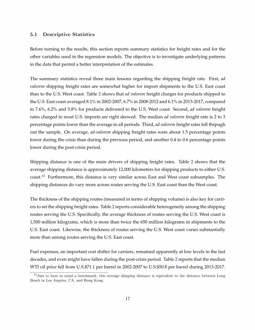
5.1 Descriptive Statistics
Before turning to the results, this section reports summary statistics for freight rates and for the
other variables used in the regression models. The objective is to investigate underlying patterns
in the data that permit a better interpretation of the estimates.
The summary statistics reveal three main lessons regarding the shipping freight rate. First, ad
valorem shipping freight rates are somewhat higher for import shipments to the U.S. East coast
than to the U.S. West coast. Table 2 shows that ad valorem freight charges for products shipped to
the U.S. East coast averaged 8.1% in 2002-2007, 6.7% in 2008-2012 and 6.1% in 2013-2017, compared
to 7.6%, 6.2% and 5.8% for products delivered to the U.S. West coast. Second, ad valorem freight
rates charged to most U.S. imports are right skewed. The median ad valorem freight rate is 2 to 3
percentage points lower than the average in all periods. Third, ad valorem freight rates fell thrpugh
out the sample. On average, ad-valorem shipping freight rates were about 1.5 percentage points
lower during the crisis than during the previous period, and another 0.4 to 0.6 percentage points
lower during the post-crisis period.
Shipping distance is one of the main drivers of shipping freight rates. Table 2 shows that the
average shipping distance is approximately 12,000 kilometers for shipping products to either U.S.
coast.43 Furthermore, this distance is very similar across East and West coast subsamples. The
shipping distances do vary more across routes serving the U.S. East coast than the West coast.
The thickness of the shipping routes (measured in terms of shipping volume) is also key for carri-
ers to set the shipping freight rates. Table 2 reports considerable heterogeneity among the shipping
routes serving the U.S. Specifically, the average thickness of routes serving the U.S. West coast is
1,500 million kilograms, which is more than twice the 650 million kilograms in shipments to the
U.S. East coast. Likewise, the thickness of routes serving the U.S. West coast varies substantially
more than among routes serving the U.S. East coast.
Fuel expenses, an important cost shifter for carriers, remained apparently at low levels in the last
decades, and even might have fallen during the post-crisis period. Table 2 reports that the median
WTI oil price fell from U.S.$71.1 per barrel in 2002-2007 to U.S.$50.8 per barrel during 2013-2017.
43Just to bear in mind a benchmark, this average shipping distance is equivalent to the distance between LongBeach in Los Angeles, CA, and Hong Kong.
17

Yet, the higher oil price volatility would have been an issue for carriers. The range in which
these prices fluctuated grew from US$50 (U.S.$35.7 to U.S.$85.5) in 2002-2007 up to nearly U.S.$60
(U.S.$44.2 to U.S.$103.1) in 2013-2017.
Finally, the average weight-to-value ratio of U.S. imports per shipment averaged 0.2 to 0.3 kilo-
grams per dollar on most shipments delivered to the U.S. regardless of the destination coast. This
ratio also decreased slightly after the global crisis from 0.25-0.27 in 2002-2007 to 0.21-0.22.
5.2 Short-run Pass-through Rates in Maritime Shipping
As explained, carriers’ rate of pass-through of costs to freight rates are key for the measurement of
shipping mark-ups. This section reports the summary statistics of the estimated short-run pass-
through rates for U.S. imports moved by sea from 2002 to 2017. It then shows estimates of how the
estimated pass-through rates are related to determinants of shipping mark-ups, such as shipping
distance and the origin country’s GDP per capita.
5.2.1 Summary Statistics of Short-run Pass-through Rates
Table 3 shows the summary statistics of the estimated short-run pass-through rates ρ.44 All
econometric techniques predict quite similar estimates for the median (average) pass-through rate
among all combinations k − c − o. For the periods before and after the crisis, all methods predict
a median pass-through rate ranging from 1.00 to 1.02, and an average rate ranging from 1.06 to
1.42.45 All three techniques thus suggest that carriers exert market power. These estimates clearly
show evidence of carriers’ ability to either pass through partially or more than completely a cost
shock to freight rates. Furthermore, they reveal that carriers’ ability mainly depends on: (1) the
product shipped; (2) the origin country, and (3) the U.S. coast of delivery.
44A problem with many estimates is that there are few data points to produce them. That is, the estimation of ρis not possible for all combinations. Some are negative and others are equal to zero. Yet, the cost of this issue isrelatively low. Table C1 shows that the value of U.S. imports through those missing combinations only account lessthan 1% of the total. Table C2 also shows that the number of products related to those combinations only represents3% to 4% of the total for the U.S. East coast and 6% to 8% of the total for the U.S. West coast. In addition, Table C3shows that the number of countries excluded from the analysis due to this issue represents 10% to 13% of the totalin the U.S. East coast and 25% to 28% of the total in the U.S. West coast.
45Table 4 shows the correlation among the estimated short-run pass-through rate retrieved from all techniques.Overall, it reaffirms that are very similar among them. Most discrepancies, though, it indicates occur among theestimated short-run pass-through rates using 2SLS versus those retrieved using OLS or the GC method.
18

Yet, the estimated short-run pass-through rates with the GC method are better grounded in sta-
tistical terms. The OLS estimates potentially suffer from endogeneity bias.46 The 2SLS estimates
reveal evidence of a weak instruments problem. The remainder of the paper relies on the GC
estimates of the short-run pass-through rates.47
The estimated pass-though rates show that, on average, carriers pass-through an increase of costs
more than completely to shipping freight charges (i.e. ρ > 1). Specifically, columns (3) and (9) in
Table 3 show that an increase of $1 in shipping costs imply a median (average) increase in ship-
ping freight charges of about $1.01 ($1.11-$1.42).48 Likewise, the distribution of these estimates,
historically ranging from 0.4 to 2.7 reaffirms that carriers ability to pass-through a cost shock to
freight charges varies significantly across products, origin country and the U.S. coast of delivery.
Hence, these estimates show that carriers have the ability to differently respond to a cost shock,
which is evidence of non-competitive conditions.49
The estimated short-run pass-through rates in this context of maritime shipping are somewhat
larger than estimates from other markets. For instance, Atkin and Donaldson (2015) estimate
an average short-run pass-through rate of 0.5 for intermediaries within the intra-national trade
markets of Nigeria, Ethiopia, and the U.S. Likewise, Bergquist (2017) estimates a pass-through
rate of 0.2 for intermediaries in the agricultural markets of sub-Saharan Africa. The average short-
run pass-through rate in the U.S. maritime shipping market is lower than the 1.6 estimated for
intermediaries in the market of residential solar power systems in California, as discussed by
Pless and Van Benthem (2017).46The GC method predicts that the correlation (%) between the FOB price and the residual estimates is higher
than 40% for half of the combinations in the U.S. East coast and higher than 25% of them in the U.S. West coast,when the pass-through rates are estimated using OLS.
47The GC method reports Confidence Intervals (CI) at 95% level to test the statistical significance. All upperbounds are positive for all ρ estimates. However, about 25% of the lower bounds are negative (See Figure 2, 3 and 4).Then, the hypothesis that ρ = 1 cannot be rejected. In order to evaluate whether this is due to overestimatedstandard errors resulted from inherent multicolinearity in the estimation, I apply the Shapiro–Wilk normality testto the FOB prices. This test reveals that two-thirds of the ρ estimates with negative CI were affected because ofthis problem. Consequently, the statistical inference might be misleading in these cases. These ρ estimates might bestatistically significant. Additionally, an evaluation of the remaining third of ρ estimates shows that it only accountfor 1.4% to 3% of the value of U.S. imports.
48This median pass-through rates near to 1 shows the identification problem when evaluating the presence of marketpower in this industry. When studies ignore carriers’ ability to pass-though a cost shock to shipping freight ratesdepending upon the shipped product and the route such as Jeon (2020), the data implicitly leads to assuming thatthis pass-through rate is equal to 1 (i.e. the average). Then, it is mistakenly claimed that conditions in this marketare competitive. However, once one considers carriers’ ability to pass through a cost shock to freight rates as I do itin this paper, all estimates indicate that conditions in the maritime shipping market are not competitive.
49As explained above, an estimated short-run pass-through equal to one implies a competitive market. Any pass-through rate below and above this mark, thus, implies that carriers extract rents from the market.
19

5.2.2 Short-run Pass-through Rates and Market Conditions
The previous section shows evidence that conditions are non-competitive in the U.S. shipping
market. Shipping carriers exert market power in this market. Given that their ability to do so
depends on product features and/or on the market conditions in each shipping route, this sec-
tion investigates under what market conditions carriers are more able to do so. Specifically, it
evaluates whether the estimated short-run pass-through rates are related to shipping distance
and origin countries’ GDP per capita. For the sake of simplicity, each relationship is estimated
non-parametrically, assuming an Epanechnikov kernel with bandwidth optimally defined by a
cross-validation process.
Figures 5 and 6 show the results of estimating the relationship between shipping distance and
short-run pass-through rates. Both figures show higher short-run pass-through rates on prod-
ucts shipped on very short routes or on medium to long shipping routes during the pre-date
and post-date period to the global recession (2008-2012). Likewise, they reveal a rough positive
relationship between carriers’ pass-through rates and shipping distance during these periods (ex-
cept for products shipped to the U.S. East coast during 2013-2017 where the relationship is much
weaker). Hence, both figures reveal two lessons. First, shipping competition is fiercer on short
to medium length shipping routes, given carriers’ lower ability to pass-though a costs shock to
freight charges. Second, this carriers’ ability increases with the shipping distance.
Figures 7 and 8 show the results of estimating the relationship between the estimated short-run
pass-through rates and origin countries’ GDP per capita. Both figures show higher pass-through
rates on products shipped from countries with lower GDP per capita to both U.S. coast. Fur-
thermore, both depict a rough negative relationship between these variables, except again by the
increasing relationship of the pass-through rates and the GDP per capita of the products shipped
to the U.S. East coast during 2013-2017. Hence, these estimates reveal that carriers passed through
a higher portion of costs to freight rates when shipping from poorer countries to the U.S.
20
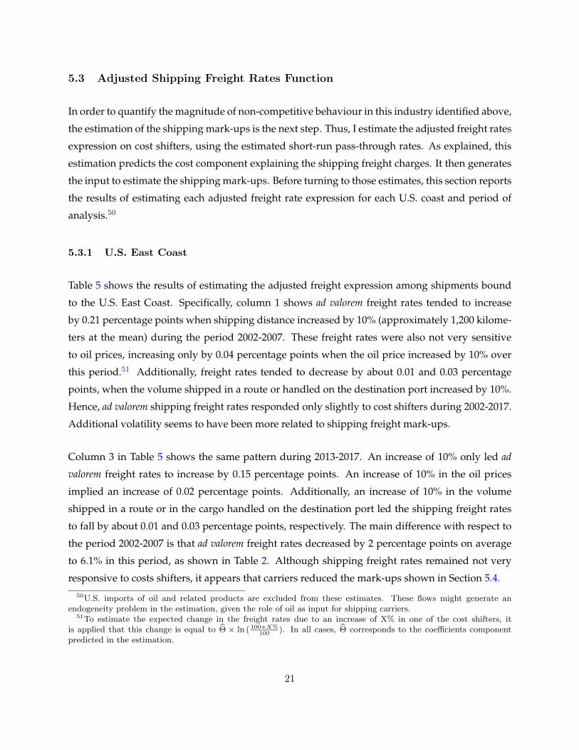
5.3 Adjusted Shipping Freight Rates Function
In order to quantify the magnitude of non-competitive behaviour in this industry identified above,
the estimation of the shipping mark-ups is the next step. Thus, I estimate the adjusted freight rates
expression on cost shifters, using the estimated short-run pass-through rates. As explained, this
estimation predicts the cost component explaining the shipping freight charges. It then generates
the input to estimate the shipping mark-ups. Before turning to those estimates, this section reports
the results of estimating each adjusted freight rate expression for each U.S. coast and period of
analysis.50
5.3.1 U.S. East Coast
Table 5 shows the results of estimating the adjusted freight expression among shipments bound
to the U.S. East Coast. Specifically, column 1 shows ad valorem freight rates tended to increase
by 0.21 percentage points when shipping distance increased by 10% (approximately 1,200 kilome-
ters at the mean) during the period 2002-2007. These freight rates were also not very sensitive
to oil prices, increasing only by 0.04 percentage points when the oil price increased by 10% over
this period.51 Additionally, freight rates tended to decrease by about 0.01 and 0.03 percentage
points, when the volume shipped in a route or handled on the destination port increased by 10%.
Hence, ad valorem shipping freight rates responded only slightly to cost shifters during 2002-2017.
Additional volatility seems to have been more related to shipping freight mark-ups.
Column 3 in Table 5 shows the same pattern during 2013-2017. An increase of 10% only led ad
valorem freight rates to increase by 0.15 percentage points. An increase of 10% in the oil prices
implied an increase of 0.02 percentage points. Additionally, an increase of 10% in the volume
shipped in a route or in the cargo handled on the destination port led the shipping freight rates
to fall by about 0.01 and 0.03 percentage points, respectively. The main difference with respect to
the period 2002-2007 is that ad valorem freight rates decreased by 2 percentage points on average
to 6.1% in this period, as shown in Table 2. Although shipping freight rates remained not very
responsive to costs shifters, it appears that carriers reduced the mark-ups shown in Section 5.4.
50U.S. imports of oil and related products are excluded from these estimates. These flows might generate anendogeneity problem in the estimation, given the role of oil as input for shipping carriers.
51To estimate the expected change in the freight rates due to an increase of X% in one of the cost shifters, itis applied that this change is equal to Θ × ln ( 100+X%
100). In all cases, Θ corresponds to the coefficients component
predicted in the estimation.
21

5.3.2 U.S. West Coast
Table 5 shows the results of estimating the adjusted freight expression for shipments delivered to
the U.S. West Coast. Column 4 reports that ad valorem freight rates charged to shipments bound for
the West coast were also not very responsive to cost shifters prior to the crisis. Ad valorem freight
rates only increased by 0.03 percentage points when oil prices increased by 10%. These freight
rates also decreased by 0.01 and 0.03 percentage points when the volume shipped in a route or
handled in the destination port increased by 10%. Interestingly, this column also reports that
Ad valorem freight rates could have even reduced by 0.11 percentage points when the shipping
distance increased by 10%. Therefore, these estimates suggest that nearly any increase in the
freight rates should be primarily attributed to changes in shipping mark-ups.
Column 6 in Table 5 shows a similar pattern during 2013-2017. Ad valorem freight rates charged for
shipments bound for the West coast remained not very responsive to cost shifters. For instance,
neither shipping distance nor the oil price can explain these freight rates. The coefficients on
these variables are not statistically significant. Ad valorem freight rates only responded to the
scale of shipping in the destination port. Column 6 shows that freight rates decreased by 0.03
percentage points when the volume handled in the destination port increased by 10%. Thus, the
main difference with respect to the period 2002-2007 was also that ad valorem freight fell by 1.8
percentage point on average to 5.8%. Additionally, carriers serving this U.S. coast also reduced
their mark-ups.
5.4 Maritime Shipping Mark-ups
Having estimated the short-run pass-through rates (ρk,co ) in Section 5.2 and ad valorem shipping
costs (T `(χk,cr )) and the maximum/minimum willingness to pay for shipping product k (ak,cod ) in
Section 5.3, maritime shipping mark-ups (µk,cr ) are calculated for every combination r−k−c−t. In
order to characterize the central tendency of these estimates, the median per shipping route (r) and
then per year (t) is calculated. This section reports the results of these estimates. Then, it reports
the results from estimating how shipping mark-ups vary with product and route characteristics.
Finally, it shows estimates from back-of-the-envelope calculations conducted to estimate the U.S.
reduction in welfare due to shipping mark-ups.
22

5.4.1 The size of Maritime Shipping Mark-ups
Table 6 shows the median shipping mark-up charged to U.S. imports of differentiated products.
Estimating all mark-ups as a share of freights charges, the first row in this table reports that the
median mark-up ranges from 34% to 43% for shipments to the U.S. East coast and from about 32%
to 34% for shipments to the U.S. West coast.52 The second and third rows also show evidence of
how sensitive mark-ups are to the short-run pass-through rates. Using the estimated short-run
pass-through rates with OLS and 2SLS models, the median mark-up ranges from 60% to 90% for
products shipped to the U.S. East coast and from almost 50% to 80% for those shipped to the
U.S. West coast.53 Thus, these estimates of the shipping mark-ups clearly show evidence of the
strong dependency of the mark-up estimates on the short-run pass-through rates. These results
also reaffirm the importance to properly econometric identification of these rates. Accordingly, the
remainder of this paper relies upon the estimated mark-ups, using the predicted short-run pass-
through rates with the GC method. As noted, the OLS estimates for ρ are subject to endogeneity
bias. The 2SLS approach does not solve the endogeneity problem, as the instruments are weak.
Examining in detail the estimated shipping mark-ups, Table 6 shows they decreased after the
global financial crisis 2008-2012. Prior to the global financial crisis, the median mark-up accounted
for 43.4% of the freight rates charged for shipping products to the U.S. East coast, and 34.2% of the
freight rates charged for shipping products to the U.S. West coast. During the post-crisis period,
though, the median mark-up only accounted for 34.1% and 32.7% of the freight rates, respec-
tively. This reduction in the mark-ups confirms the tough market conditions that carriers faced
52As noted, shipping mark-ups are estimated as a Lerner (1934) index. Accordingly, these mark-ups are alwayspositive, assuming a negative inverse demand elasticity (η) (See expression (13)). However, this is a puzzle in theshipping industry. About 20% to 25% of the estimated mark-ups on shipments to the U.S. East coast and 30%to 36% of those charged on shipments to the U.S. West coast are negative. It appears that mode switching in thetransportation market may lead freight markets to have a positive elasticity for a single mode. Given that shippingproducts by air is very sensitive to fuel prices (Hummels et al., 2014), this elasticity can be positive for productsthat more often switch among modes of transportation. The rationale is simple. A negative (positive) shock inthe fuel prices tends to more drastically increase (decrease) the cost of freight by air than the costs of shipping viaother modes of transportation. Thus, the demand for other modes of shipping services may increase (decreases),despite the cost of freight via those modes also increases (decreases). I mainly attribute to this puzzle the estimatednegative mark-ups. However, I acknowledge that these mark-ups might be also explained by excessive shippingcapacity, subventions for shipping products or even insufficient observations for estimating the mark-ups for somecombinations (origin-destination-product-year).
53Preliminary versions of this paper predicted a median maritime shipping mark-up of about 30% to 38% whenestimating the short-run pass-through rates with OLS and 2SLS. The difference with respect to these updatedestimates is due to the fact that in the estimation of adjusted freight function considers: (1) the volume handled in adestination port, and (2) the consumers preferences for products from a particular origin country. Two modificationincorporated to the adjusted freight function aimed to improve the identification of the shipping costs, and so of theshipping mark-ups.
23

after the crisis (GSF Global Shippers Forum, 2017; ICS International Chamber of Shipping, 2017;
Samunderu, 2018). It clearly show that carriers reduced the rents extracted from the market, given
that freight charges also decreased. These estimates also show that the difference between the
median mark-up charged for shipping products to both U.S. coasts diminished from 9 percentage
points of the freight rates prior to the global financial crisis to 1.5 percentage point during the
post-crisis period.54
At the country level, Table 7 does not show an overall pattern during the period 2002-2017. Av-
erage shipping mark-ups per country tended to be apparently conditional on the U.S. coast to
which carriers ship the products. For instance, columns 1-3 show that carriers serving the U.S.
East coast reduced relatively more their mark-ups during 2013-2017 on shipments from Asian
countries (such as Japan and Vietnam) than on shipments from European countries (such as Ger-
many and United Kingdom). In contrast, columns 4-6 show that carriers serving the U.S. West
coast reduced the mark-ups charged on shipments from Asian countries (such as China, Taiwan
and Vietnam) during this period, but they raised the mark-up on shipments from European coun-
tries (such as Germany United Kingdom and Italy). Additionally, Table 8 and Table 9 show that
carriers charge higher mark-ups when delivering products to larger U.S. customs districts such as
New York, NY, and Houston, TX, in the U.S. East coast and Los Angeles, CA, Seattle, WA and San
Francisco, CA, in the U.S. West coast. These estimates thus offer anecdotal evidence that larger
mark-ups are charged on routes with bigger destination ports.
5.4.2 Evaluating the Predicted Shipping Mark-ups
In order to investigate whether non-competitive behavior in the maritime shipping market dis-
proportionately affects developing and distant countries, I estimate reduced-form models of the
ad valorem shipping freight rates fk`,r, ad valorem shipping mark-ups µ`,kr , and the tariff equivalent
of these mark-ups τ `,kµr on the following variables: (1) the shipping distance on a route, DISTr; (2)
the origin country’s GDP per capita, GDPpcot; and (3) the substitution elasticity of each product
σk (estimated by Soderbery (2015)).55
54As explained, these shipping mark-ups estimates merely correspond to median mark-up charged within a routein a particular year. Thus, this does not imply that carriers charge these mark-ups to all products. These are justpoint estimates, calculated as an median, from the estimated shipping mark-ups at the product and route level overtime.
55The estimated negative mark-ups are excluded from this estimation. These product-country pair might add noiseand some endogeneity to the estimation.
24

Table 10 shows the results of this estimation. As shown, all estimates are very robust and predict
the same conclusions in all periods.56 First, ad valorem freight rates are higher for products shipped
from developing and distant countries to the U.S. (See Columns 1-2, 7-8 and 13-14). Doubling
GDP per capita reduces shipping freight rates by 9 to 11 percent.57 Shipping freight rates also
increase about 1.8 to 2.2 percent (i.e. about 0.12 percentage points) for every 1,200 kilometers of
extra shipping distance.58 Second, freight mark-ups are higher relative to freight rates charged
when shipping products from developed and closer countries to the U.S (See Columns 3-4, 9-10
and 15-16). Doubling GDP per capita increases ad valorem mark-ups to freight charges by 2 to
3 percent (i.e. almost one percentage point). Likewise, reducing the shipping distance by 10%
increases ad valorem mark-ups by 0.6 to 0.7 percent. Finally, shipping mark-ups represent a higher
tariff equivalent on products shipped from developing and distant countries (See columns 5-6,
11-12 and 17-18). Specifically, these estimates show that halving GDP per capita increases the
tariff equivalent of mark-ups approximately by 8 to 11 percent (equivalent to 0.1 to 0.3 percentage
points). Likewise, doubling the shipping distance raises this equivalent tariff by 8 to 13 percent
(equivalent to 0.1 to 0.3 percentage points).
5.4.3 Counterfactual Calculations
To investigate how shipping mark-ups affect import prices, I apply the estimated mark-ups to the
freight rates in order to decompose it between marginal shipping costs and shipping mark-ups.
This exercise yields that for each U.S.$5.5 to U.S.$6.3 paid at the median for shipping U.S.$100
of differentiated products to the U.S. during 2002-2007, U.S.$2.1 to $2.6 corresponded to shipping
mark-ups (See Figure 9). Likewise, for each U.S.$3.9 to U.S.$4.5 paid for shipping the same amount
of merchandise during 2013-2017, about U.S.$1.4 of this constituted mark-ups. Thus, maritime
shipping mark-ups represented an equivalent ad valorem tariff ranging from 2.1% to 2.6% during
2002-2007 and of 1.4% during 2013-2017. These estimates are roughly equivalent to one to two-
thirds of the average U.S. tariff during this period, which ranged from 2.8% to 4.0% (World-Bank,
2021).56To estimate the expected change in the freight rates and shipping mark-ups due to an increase of X% in the
shipping distance or the GDP per capita, it is applied that this change is equal to exp (Θ× ln ( 100+X%100
))− 1. In all
cases, Θ corresponds to the coefficients component predicted on the estimation.57Approximately, this accounts for 0.6 percentage points of the freight rates, assuming an ad valorem freight rate
of about 6%.581,200 kilometers is equivalent to an increase of 10% in the average shipping distance.
25

5.4.4 The Effects of Shipping Mark-ups on International Trade Flows and Welfare
In order to determine what the non-competitive pricing behavior in the maritime shipping indus-
try implies for trade and welfare, I conduct two additional exercises. First, the trade elasticity is
used to determine the response of U.S. imports to the implicit costs of the estimated mark-ups.
Second, back-to-the envelope calculations apply the trade elasticity in order to estimate the wel-
fare loss resulting from the maritime shipping mark-ups.
Most structural gravity models show that the response of trade flows to trade costs largely de-
pends on the assumed trade elasticity.59 Many gravity studies thus estimate trade elasticities
ranging from 5 to 10 Anderson and van Wincoop (2004). Recent estimates also imply a smaller
elasticity, ranging from 3 to 5, and estimates of this elasticity in shipping markets find that it is
equal to 3 (Simonovska and Waugh, 2014; Wong, 2017).60 Using the previous result that shipping
mark-ups accounted for an equivalent ad valorem tariff ranging from 2.1% to 2.6% during 2002-
2007 and of 1.4% during 2013-2017, this paper estimates that U.S. imports would have been 7.0%
to 11.6% greater in 2002-2007 and 4.2% to 6.1% in 2013-2017 if mark-ups were set to zero (See
Table 11).
In terms of welfare, the loss attributed to non-competitive behavior in the maritime shipping in-
dustry can be estimated by applying the approach of Arkolakis et al. (2012). That paper shows
that the change in welfare (W ) due to a foreign shock can be computed as λ−1/ε, regardless of the
micro-level implications of a model; where λ is the change in the share of domestic expenditure
and ε is the trade elasticity. Thus, the welfare loss of shipping mark-ups for U.S. can be easily
calculated as follows, comparing trade flows with and without shipping mark-ups.
W = λ−1/εmark−ups − λ
−1/εNOmark−ups (16)
Using the fact that U.S. import penetration ranged from 12.5% to 16.6% during 2002-2017 and pre-
dicting that it would have been 13.1% to 17.2% in a scenario without mark-ups for differentiated
products, λmark−ups would average 83.4%-87.5%, and λNOmark−ups would average 82.8%-86.9%.
Equation (16) implies that U.S. consumers perceived an average loss of about 0.1%-0.2% in their
real income during 2002-2017 due to the shipping mark-ups, assuming a trade elasticity ε between
59Simonovska and Waugh (2014) survey most of these studies.60These studies though do not consider the non-competitive behavior in the shipping market on these estimates.
26

3 and 5 (See Table 12). As a point of reference, this loss would be about two-thirds of the 0.3%
estimated cost to consumers of the U.S.-China trade war (Fajgelbaum et al., 2019).
5.4.5 Did the 2008-2012 Global Financial Crisis Affect Carriers’ Ability to Exert
Market Power?
The estimation strategy employed in this paper assumes parameter stability within the period
of study. Assuming stability during the global financial crisis period (2008-2012) is questionable.
Global aggregate demand for goods and services was seriously distorted. Some shipping costs for
carriers (e.g. oil prices) reached atypical levels, and unused capacity in the market significantly
increased during this period (UNCTAD, 2017).61 This is, however, a period of significant interest.
Thus, in order to inform our understanding of the effects of the crisis, I apply the same estimation
strategy to the period 2008-2012.
Applying the same estimation strategy to 2008-2012 indicates that carriers’ ability to transfer a cost
shock to freight rates slightly decreased during 2008-2012 period. Columns (3) and (6) in Table 3
show that the average pass-through rate decreased from 1.42 in 2002-2007 to 1.10 in 2008-2012
on shipments to the U.S. East coast, and from 1.11 in 2002-2007 to 1.06 in 2008-2012 on those to
the U.S. West coast. So, carriers were unable to keep transferring the same proportion of costs
to freight charged on the products to which they transferred the most in 2002-2007. This result
reinforces the thesis that shipping carriers faced tough conditions during this period (GSF Global
Shippers Forum, 2017; ICS International Chamber of Shipping, 2017; Samunderu, 2018).
Column (2) in Table 5 also shows that oil price volatility slightly affected shipping carriers during
this period, especially to those serving the U.S. East coast. An increase of 10% in the oil price
during 2008-2012 implied an increase of 0.35 percentage pointsin the shipping freight rates. That
is, the response in ad valorem freight rates of changes to prices was approximately 10 times larger
than during 2002-2007. In contrast, Column (2) and (5) in Table 5 show that an increase of 10% in
the shipping volume in a route or the volume handled in a destination port continued to lead a
reduction in freight rates of 0.1-0.3 percentage points.
61Table 2 shows that, during the crisis period, ad valorem freight rates (fk`,r) decreased to 6.2%-6.7%, 1.5 percentagepoints lower than in the period 2002-2007. The average volume of goods shipped also fell by 10.2% in routes to theU.S. East coast and by 5.6% in routes to the U.S. West coast. Likewise, important cost shifters for shipping carrierssuch as oil prices were very volatile. Oil prices decreased to almost US$40 per barrel in 2009. Then, reversing theircourse these prices touched the barrier of US$120 in 2011 and oscillated around US$90 to US$100 afterwards.
27

Estimates in Table 6 indicate that carriers significantly reduced their mark-ups during the crisis.
Specifically, ad valorem shipping mark-ups (µ`,kr ) fell from 43.4% on average in 2002-2007 to 38.2%
in 2008-2012 for differentiated products shipped to the U.S. East coast, and from 34.2% to 27.5%
for products shipped to the U.S. West coast. That is, the equivalent ad valorem tariff decreased
from 2.1%-2.6% to 1.3%-1.8%. In the post-crisis period, mark-ups of shipments to the U.S. East
coast fell even further (to 34.1%), and rose slightly (to 32.7%) on shipments for the U.S. West coast.
All these results reveal two main lessons for the period of global crisis (2008-2012). Shipping costs
were volatile costs, and carriers reduced their market power. Two outcomes that estimates show
persisted during the post-crisis period, as explained above.
5.5 Robustness exercises
In order to quantify the effect of non-competitive pricing behavior in the maritime shipping indus-
try, this paper applies a modified version of Atkin and Donaldson (2015). To this aim, it uses U.S.
import data at HS6-digit code level, as is standard most trade studies. One concern regarding this
level of product aggregation is whether the Alchian-Allen effect undermines the identification of
the estimated short-run pass-through rates and so of the shipping mark-ups. Hummels and Skiba
(2004) show that transport costs affect the quality-composition of the traded good. So, if the qual-
ity variation across the products within each HS6-digit level is sufficiently large, estimates at HS6
level could be biased. In order to test the robustness of the previous estimates for the short-run
pass-through rates and the shipping mark-ups, all models are also estimated using U.S. imports
at HS10-digit product level.
This robustness exercise shows that estimated short-run pass-through rates (ρ) are robust to dis-
aggregation of the U.S. import data to the HS10 level.62 The correlation between the estimated
short-run pass-through rates using data at HS6 digit-code versus the average of those estimated
using data at HS10 digit code ranges between 66% to 78%. Likewise, a graphical analysis, in
which both sets of short-run pass-through rates are plotted along with a solid 45-degree line, also
indicates that the estimated short-run pass-through rates are stable surrounding this solid line;
regardless the level of aggregation of the U.S. imports data (See Figure D1 and Figure D2). Most
62To this particular exercise, I previously removed outlier estimates for ρ in order to reduce the noise in thisestimation. To so so, I set 30 as the highest feasible level, which is roughly 10 times the percentile 90 of theestimated ρ. This exercise implied dropping about 40 observations out of approximately 50,000 observation in thesubsample for the U.S. East coast, and 30 observations out of the 28,000 in the subsample of the West coast.
28

discrepancies appear to be related to some extremely high short-run pass-through rates estimated
for HS10 digit products. Larger variance in the HS10-digit level data is expected, given the smaller
number of observations used to estimate the HS10 level short-run pass-through rates.
Table D1 also reinforces this result, showing that the distribution of both sets of short-run pass-
through rates is similar. The median short-run pass-through rate in both distributions is 1.01.
Both distributions also have their minimum values around 0.4. The main difference between both
distributions is that the average short-run pass-through rate is higher in about 0.2 points when es-
timated at HS10 than at HS6. Thus, the Alchian-Allen effect would be leading to underestimating
carriers’ ability to pass-through a cost shock to freight rates.
Another important concern is whether the estimated maritime shipping mark-ups µ are also ro-
bust. To evaluate this issue, the maritime shipping mark-ups are calculated using the estimated
short-run pass-through rates for HS10 product codes. Table D2 shows that the estimated mark-ups
are very robust overall in terms of magnitude. Regardless of the level of product disaggregation,
the median shipping mark-up is about one third of the shipping freight charges. Likewise, the
HS10 estimates confirm that mark-ups were higher before the global financial crisis. Neverthe-
less, columns (1)-(2) show that the median shipping mark-up on shipments to the U.S. East coast
is about 5 to 6 percentage points lower, when is calculated using data at HS10 product-code than
with data at HS6 product-code. Likewise, columns (3)-(4) show that the median mark-ups on
shipments to the U.S. West coast differ in about 3 percentage points, when is calculated using data
at HS10 product-code than with data at HS6 product-code.
Finally, the revision of the SITC codes in the U.S. census concordances–used to merge the Rauch
product classification–is unclear for the years 2002-2015.63 So, I assume that all SITC codes were
at Revision 2, in order to circumvent the methodological problem of having SITC codes classified
as both differentiated and homogeneous, when some codes were converted from Revision 4 to Re-
vision 2. Thus, in order to evaluate the robustness of all estimates to this assumption, all estimates
were calculated again assuming that all SITC codes were at Revision 4. This exercise shows that
all estimates are very robust to the assumed revisions for the SITC codes. For instance, Table D3
shows that the median pass-through rate ranges continue to center around 1.01, and the average
ranges from 1.1 to 1.6. Similarly, Table D4 indicates that the maritime shipping mark-ups are also
very similar, assuming Revision 4 for the SITC codes. Specifically, shipping mark-ups continue to
63See Section 3, footnote 27.
29

account for approximately one-third of the freight charges.
6 Conclusion
This paper quantifies the effect of non-competitive pricing behavior in the maritime shipping in-
dustry on (1) total freight costs, (2) the volume of international trade, and (3) economic welfare.
It also evaluates whether non-competitive behavior disproportionately affects developing and/or
distant countries. Using U.S. import data, the method of Atkin and Donaldson (2015) is applied
to the maritime shipping industry. This permits estimating the shipping mark-ups charged on
freight charges for periods 2002-2007, 2008-2012, and 2013-2017.
The method of Atkin and Donaldson (2015) solves the theoretical problem of separately identify-
ing firms’ marginal costs and mark-ups. Following a two-step procedure, the pass-through rate
of marginal costs to freight rates is first estimated for most imported products to the U.S. Then,
an adjusted expression for shipping freight rates is estimated using the estimated short-run pass-
through rates from the first stage. Finally, shipping mark-ups are calculated as a standard Lerner
(1934) index, using previous estimates.
The estimated short-run pass-through rates of shipping cost to freight rates reaffirm previous em-
pirical evidence of imperfect competition in the maritime shipping industry. Furthermore, the
distribution of these pass-though rates reveals that carriers do not exert market power evenly.
Carriers extract larger rents when shipping products for which they can pass through more than
completely a cost shock to their freight (about half of the products). Likewise, they do the same
when shipping products with partial pass-through rates. The difference, in this second case, is
that carriers are forced to reduce their mark-ups whenever there is a positive cost shock.
This paper also estimates that maritime shipping mark-ups represent approximately one third of
shipping freight charges on U.S. imports. Specifically, it shows that these margins range from 34%
to 43% of freight charges on shipments delivered to the U.S. East coast and from 32% to 34% on
those delivered to the U.S. West coast. Likewise, it finds evidence that shipping carriers charge
higher mark-ups on shipments delivered to U.S. ports that handle large flows of imports
Putting these results in context, this paper estimates that maritime shipping mark-ups represent
an ad valorem tariff for differentiated products ranging from 1.4% to 2.6%. These are similar in
30

magnitude to average ad valorem tariffs in the U.S. from the last two decades. Using trade elas-
ticities from the literature, the estimates imply that U.S. imports would have been approximately
4.2% to 11.6% higher if these mark-ups were set equal to zero. The implied welfare costs of mark-
ups for U.S. consumers is an annual reduction of approximately 0.1%-0.2% of their real income. In
addition, estimated mark-ups are larger for shipments from poorer, and more distant countries.
31

References
Amjadi, A. and A. Yeats (1995). Have Transport Costs Contributed to the Relative Decline ofSub-Saharan African Exports? Policy Research, Working Paper 1558, World Bank, Washington,D.C.
Anderson, J. E. and E. van Wincoop (2004). Trade Costs. Journal of Economic Literature 42(3), 691–751.
Ardelean, A. and V. Lugovskyy (2018). Firm-level heterogeneity in International Transport Costs:Evidence from Chile. Mimeo.
Arkolakis, C., A. Costinot, and A. Rodriguez-Clare (2012). New Trade Models, Same Old Gains?American Economic Review 102(1), 94–130.
Armington, P. S. (1969). A Theory of Demand for Products Distinguished by Place of Production.Staff Papers 16(1), 159–178.
Asturias, J. (2019). Endogenous transportation costs. [Revise and Resubmit, European EconomicReview].
Atkin, D. and D. Donaldson (2015). Who’s Getting Globalized? The Size and Implications ofIntra-National Trade Costs. [Revise and Resubmit, Econometrica].
Balassa, B. (1965). Trade Liberalisation and “Revealed” Comparative Advantage. The ManchesterSchool 33(2), 99–123.
Bergquist, L. F. (2017). Pass-through, Competition, and Entry in Agricultural Markets: Experi-mental Evidence from Kenya. [Revise and Resubmit, American Economic Review].
Brancaccio, G., M. Kalouptsidi, and T. Papageorgiou (2020). Geography, transportation, and en-dogenous trade costs. Econometrica 88(2), 657–691.
Broda, C. and D. E. Weinstein (2006). Globalization and the Gains from Variety. The QuarterlyJournal of Economics 121(2), 541–585.
Bryan, I. (1974). Regression Analysis of Ocean Liner Freight Rates on some Canadian ExportRoutes. Journal of Transport Economics and Policy 8(2), 161–173.
Bulow, J. I. . and P. Pfleiderer (1983). A Note on the Effect of Cost Changes on Prices. Journal ofPolitical Economy 91(1), 182–185.
Clark, X., D. Dollar, and A. Micco (2004). Port Efficiency, Maritime Transport Costs, and BilateralTrade. Journal of Development Economics 75(2), 417–450.
Clyde, P. S. and J. D. Reitzes (1998). Market Power and Collusion in the Ocean Shipping Industry:Is a Bigger Cartel a Better Cartel? Economic Inquiry 36(2), 292–304.
Davies, J. (1986). The Theory of Contestable Markets and its Application to the Liner Shipping Industry.Canadian Transport Commission, Research Branch, Transport Industries Analysis.
Devanney III, J. W., V. Livanos, and R. Stewart (1975). Conference Ratemaking and the West Coast
32

of South America. Journal of Transport Economics and Policy 9(2), 154–177.
Fabinger, M. and E. G. Weyl (2012). Pass-Through and Demand Forms. University of Chicago.Mimeo.
Fajgelbaum, P. D., P. K. Goldberg, P. J. Kennedy, and A. K. Khandelwal (2019). The Return to Pro-tectionism. National Bureau of Economic Research - NBER, Working Paper 25638, Cambridge,MA.
Feenstra, R. C. (1994). New Product Varieties and the Measurement of International Prices. TheAmerican Economic Review, 157–177.
Fink, C. (2002). Trade in International Maritime Services: How Much Does Policy Matter? TheWorld Bank Economic Review 16(1), 81–108.
GSF Global Shippers Forum (2017). 6th Annual Report. Technical Report October, Global Ship-pers’ Forum, Kent, UK.
Heaver, T. D. (1973). The Structure of Liner Conference Rates. The Journal of Industrial Eco-nomics 21(3), 257–265.
Hoffmann, J. and S. Kumar (2013). Globalisation–The Maritime Nexus. In The Handbook of MaritimeEconomics and Business, pp. 65–94. Informa Law from Routledge.
Hummels, D. (2007). Transportation Costs and International Trade in the Second Era of Globaliza-tion. Journal of Economic Perspectives 21(3), 131–154.
Hummels, D., R. Jørgensen, J. Munch, and C. Xiang (2014). The Wage Effects of Offshoring: Evi-dence from Danish Matched Worker-Firm Data. American Economic Review 104(6), 1597–1629.
Hummels, D., V. Lugovskyy, and A. Skiba (2009). The Trade Reducing Effects of Market Power inInternational Shipping. Journal of Development Economics 89(1), 84–97.
Hummels, D. and A. Skiba (2002). A Virtuous Circle? Regional Tariff Liberalization and ScaleEconomies in Transport. Purdue University. Mimeo.
Hummels, D. and A. Skiba (2004). Shipping the Good Apples Out? An Empirical Confirmation ofthe Alchian-Allen Conjecture. Journal of Political Economy 112(6), 1384–1402.
Hummels, D. L. and G. Schaur (2013). Time as a Trade Barrier. American Economic Review 103(7),2935–59.
ICS International Chamber of Shipping (2017). 2017 Annual Review. Technical report, GlobalShipping Industry, London.
Jeon, J. (2020). Learning and investment under demand uncertainty in container shipping.Manuscript, Department of Economics, Boston University.
Korinek, J. and P. Sourdin (2009). Maritime Transport Costs and Their Impact on Trade. Organi-zation for Economic Co-operation and Development TAD/TC/WP (2009)7.
Lerner, A. P. (1934). The Concept of Monopoly and the Measurement of Monopoly Power. The
33
Review of Economic Studies 1(3), 157–175.
Limao, N. and A. J. Venables (2001). Infrastructure, Geographical Disadvantage, Transport Costs,and Trade. The World Bank Economic Review 15(3), 451–479.
Martınez-Zarzoso, I., E. M. Perez-Garcıa, and C. Suarez-Burguet (2008). Do Transport Costs havea Differential Effect on Trade at the Sectoral Level? Applied Economics 40(24), 3145–3157.
Micco, A. and N. Perez (2001). Maritime Transport Costs and Port Efficiency. In Seminar ”TowardsCompetitiveness: The Institutional Path”. Santiago, Chile: IDB. Citeseer.
Park, S. and S. Gupta (2012). Handling endogenous regressors by joint estimation using copulas.Marketing Science 31(4), 567–586.
Pless, J. and A. A. Van Benthem (2017). The Surprising Pass-Through of Solar Subsidies. NationalBureau of Economic Research - NBER, Working Paper 23260, Cambridge, MA.
Radelet, S. and J. D. Sachs (1998). Shipping Costs, Manufactured Exports, and Economic Growth.Harvard Institute for Economic Development. Mimeo.
Rauch, J. E. (1999). Networks Versus Markets in International Trade. Journal of International Eco-nomics 48(1), 7–35.
Samunderu, E. (2018). The Maritime Container Transportation Chain (MCTC). In R. Neise (Ed.),Container Logistics: The Role of the Container in the Supply Chain, Chapter ONE, pp. 11–30.
Sanchez, R. J., J. Hoffmann, A. Micco, G. V. Pizzolitto, M. Sgut, and G. Wilmsmeier (2003). Port Ef-ficiency and International Trade: Port Efficiency as a Determinant of Maritime Transport Costs.Maritime Economics & Logistics 5(2), 199–218.
Simonovska, I. and M. E. Waugh (2014). The elasticity of trade: Estimates and evidence. Journal ofinternational Economics 92(1), 34–50.
Soderbery, A. (2015). Estimating import supply and demand elasticities: Analysis and implica-tions. Journal of International Economics 96(1), 1–17.
UNCTAD (2017). Review of Maritime Transport 2017. New York and Geneva: UNITED NATIONSPUBLICATION.
Weyl, E. G. and M. Fabinger (2013). Pass-Through as an Economic Tool: Principles of Incidenceunder Imperfect Competition. Journal of Political Economy 121(3), 528–583.
Wilmsmeier, G. and J. Hoffmann (2008). Liner Shipping Connectivity and Port Infrastructure asDeterminants of Freight Rates in the Caribbean. Maritime Economics & Logistics 10(1-2), 130–151.
Wilmsmeier, G., J. Hoffmann, and R. J. Sanchez (2006). The Impact of Port Characteristics onInternational Maritime Transport Costs. Research in Transportation Economics 16, 117–140.
Wong, W. F. (2017). The Round Trip Effect : Endogenous Transport Costs and International Trade.World Trade Organization, Geneva, Switzerland.
World-Bank (2021). Database, Statistics, World Development Indicators - WB-WDI.
34

7 Tables
Table 1: Ad-Valorem Freight Charges from China and Loading Cargo of U.S. Imports to U.S. Portslocated in U.S. West Coast - 2017
Seattle Los Angeles San Francisco
Panel A.
Ad-Valorem Freight ChargesCell Phones 0.7% 0.8% 5.2%Televisions 1.9% 2.3% 2.8%Bicycles 5.4% 6.5% 8.1%Car Tires 14.0% 13.5% 14.0%
Panel B.
Number of Transactions (Millions) 15 107 19Total Volume Imported (Million tons) 154 995 425Total Value Imported - FOB (US$ Billion) 508 3,116 566
Note: HS6 digit-codes used for these calculations are: cellphones, 85.17.12; televisions, 85.28.72;bicycles, 82.12.00; and car tires; 40.11.10. Ad Valorem freight rates are calculated using U.S.Merchandise Imports Database. The number of transactions corresponds to the number of cardsreported in the U.S. Merchandise Imports Database
35

Table 2: Summary Statistics - Key Variables in U.S. Maritime Shipping Market - Differentiated Products
2002-2007
U.S. East Coast U.S. West Coast
Obs. Mean Median Std. Dev. Perc. 1% Perc. 99% Obs. Mean Median Std. Dev. Perc. 1% Perc. 99%
Ad Valorem Freight Rate† 931,501 8.1 5.1 11.9 0.0 49.5 334,177 7.6 4.8 11.1 0.0 46.0Shipping Distance‡ 931,501 12,089 9,028 6,023 1,733 21,832 334,177 12,020 12,167 2,558 5,048 17,855Shipping Volume - Route∗ 931,501 703 234 1,438 0 5,843 334,177 1,444 294 3,616 0 20,945Oil Price? 931,501 61.6 71.1 18.9 35.7 85.5 334,177 61.7 71.1 18.9 35.7 85.5Ratio Weight-to-Value∓ 931,501 0.25 0.09 3.02 0.00 2.06 334,177 0.27 0.09 18.34 0.00 1.94
2008-2012
U.S. East Coast U.S. West Coast
Obs. Mean Median Std. Dev. Perc. 1% Perc. 99% Obs. Mean Median Std. Dev. Perc. 1% Perc. 99%
Ad Valorem Freight Rate† 749,548 6.7 4.1 11.2 0.0 42.9 263,635 6.2 3.8 10.0 0.0 39.3Shipping Distance‡ 749,548 12,238 9,093 5,999 1,733 21,832 263,635 12,015 12,167 2,513 5,463 17,481Shipping Volume - Route∗ 749,548 631 201 1,231 0 5,790 263,635 1,363 256 3,482 0 16,835Oil Price? 749,548 95.8 100.4 14.5 70.8 113.5 263,635 95.9 100.4 14.5 70.8 113.5Ratio Weight-to-Value∓ 749,548 0.21 0.08 2.57 0.00 1.78 263,635 0.20 0.08 0.68 0.00 1.69
2013-2017
U.S. East Coast U.S. West Coast
Obs. Mean Median Std. Dev. Perc. 1% Perc. 99% Obs. Mean Median Std. Dev. Perc. 1% Perc. 99%
Ad Valorem Freight Rate† 829,324 6.1 3.7 9.7 0.0 40.3 277,467 5.8 3.6 9.0 0.0 38.1Shipping Distance‡ 829,324 12,046 8,832 5,925 1,782 21,832 277,467 12,120 12,551 2,529 5,394 17,481Shipping Volume - Route∗ 829,324 687 252 1,231 0 6,724 277,467 1,565 296 3,998 0 19,741Oil Price? 829,324 68.1 50.8 25.1 44.2 103.1 277,467 68.6 50.8 25.3 44.2 103.1Ratio Weight-to-Value∓ 829,324 0.21 0.08 1.48 0.00 1.88 277,467 0.22 0.09 1.97 0.00 1.80
†: ad valorem freight rate charged in the origin country o for shipping product k to the U.S. Customs district d in year t.‡: maritime shipping distance (in kilometers) for delivering product k from country o to the U.S. Customs district d.∗: total shipping volume (in million of kilograms) from origin country o to the U.S. Customs district d in year t.?: WTI oil price (in U.S.$ prices of 2017) in year t.∓: ratio weight-to-value of product k shipped from country o to the U.S. Customs district d in year t (in kg/U.S.$ prices of 2017).
36

Table 3: Summary Statistics - Short Run Pass Through-Rate ρ
U.S. East Coast
2002-2007 2008-2012 2013-2017
OLS 2SLS GC OLS 2SLS GC OLS 2SLS GC
(1) (2) (3) (4) (5) (6) (7) (8) (9)
Mean 1.09 1.10 1.42 1.07 1.14 1.10 1.06 1.10 1.16Median 1.02 1.02 1.01 1.02 1.01 1.01 1.01 1.01 1.01Std Deviation 1.30 2.04 31.98 1.22 4.23 2.73 0.77 3.55 9.78Percentile 1% 0.59 0.49 0.43 0.60 0.49 0.44 0.62 0.51 0.46Percentile 99% 2.00 2.26 2.71 1.94 2.36 2.54 1.91 2.26 2.47Number Obs. 44,555 42,966 55,212 39,642 37,474 48,578 42,914 41,400 52,277
U.S. West Coast
2002-2007 2008-2012 2013-2017
OLS 2SLS GC OLS 2SLS GC OLS 2SLS GC
(1) (2) (3) (4) (5) (6) (7) (8) (9)
Mean 1.09 1.10 1.11 1.06 1.36 1.06 1.12 1.14 1.13Median 1.02 1.02 1.01 1.01 1.01 1.00 1.01 1.01 1.00Std Deviation 1.77 1.85 3.14 1.73 41.62 1.73 8.86 9.09 8.61Percentile 1% 0.58 0.51 0.46 0.58 0.52 0.44 0.61 0.51 0.46Percentile 99% 1.90 2.11 2.30 1.78 2.07 2.09 1.81 2.11 2.14Number Obs. 27,971 26,992 31,823 24,398 23,112 27,520 25,603 24,673 28,819
37

Table 4: Correlation of the estimated Short-run Pass Through-Rates among econometric techniques
U.S. East Coast U.S. West Coast
2002-2007 OLS 2SLS GC OLS 2SLS GC
OLS 1.000 OLS 1.0002SLS 0.695 1.000 2SLS 0.972 1.000GC 0.996 0.691 1.000 GC 0.998 0.970 1.000
2008-2012 OLS 2SLS GC OLS 2SLS GC
OLS 1.000 OLS 1.0002SLS 0.308 1.000 2SLS 0.043 1.000GC 0.996 0.307 1.000 GC 0.998 0.042 1.000
2013-2017 OLS 2SLS GC OLS 2SLS GC
OLS 1.000 OLS 1.0002SLS 0.486 1.000 2SLS 0.997 1.000GC 0.991 0.477 1.000 GC 1.000 0.997 1.000
38

Table 5: Adjusted Ad-Valorem Freight Rates Function
U.S. East Coast U.S. West Coast
2002-2007 2008-2012 2013-2017 2002-2007 2008-2012 2013-2017
(1) (2) (3) (4) (5) (6)
log (Distance) 0.0342*** -0.00438 -0.00248 -0.0365** -0.00633 0.0363(0.00446) (0.00861) (0.00421) (0.0152) (0.0244) (0.0313)
log (Oil Price) 0.0325*** -0.0219 -0.0327*** -0.0545* 0.0300 0.117(0.00837) (0.0179) (0.00766) (0.0315) (0.0490) (0.0764)
log (Distance) × log (Oil Price) -0.00299*** 0.00385** 0.00366*** 0.00614* -0.00210 -0.0123(0.000899) (0.00189) (0.000826) (0.00338) (0.00526) (0.00816)
log (Weight/Value) 0.0120*** 0.00817*** 0.00827*** 0.0111*** 0.0112*** 0.00976***(0.000743) (0.00103) (0.000689) (0.000933) (0.000901) (0.00124)
log (Vol. Route) -0.00135*** -0.00113*** -0.000934*** -0.000996** -0.00161*** -0.000151(0.000249) (0.000230) (0.000228) (0.000387) (0.000471) (0.00118)
log (Vol. Destination Port) -0.00356*** -0.00304*** -0.00289*** -0.00356*** -0.00201*** -0.00385***(0.000369) (0.000374) (0.000296) (0.000429) (0.000524) (0.000965)
constant -0.0871** 0.187** 0.226*** 0.630*** 0.243 -0.0897(0.0404) (0.0798) (0.0388) (0.141) (0.228) (0.277)
N 873,922 700,917 778,280 296,375 231,678 244,074R-sq 0.996 0.993 1.000 1.000 0.999 0.995
Standard errors in parenthesis clustered by product-origin country, product-year and product-U.S. customs district of entry.*p < 0.1, **p < 0.05, ***p < 0.01Note: these model excludes the imports of oil and related products, pooled on the HS2 digit-code sector 27.
39

Table 6: Median Maritime Shipping Mark-ups(% of Maritime Shipping Freight Charges)
U.S. East Coast U.S. West Coast
2002-2007 2008-2012 2013-2017 2002-2007 2008-2012 2013-2017
(1) (2) (3) (4) (5) (6)
Gaussian Copula 43.4 38.2 34.1 34.2 27.5 32.7OLS 86.6 71.0 71.5 74.7 77.7 74.52SLS 83.0 67.6 61.3 48.9 65.0 65.9
Note: columns (1)-(6) report the median ad valorem mark-ups to maritime shipping freightrates across HS6-digit products and shipping routes.
Table 7: Median Maritime Shipping Mark-ups per Origin Country(% of Maritime Shipping Freight Charges)
U.S. East Coast U.S. West Coast
Avg. Share Imports 2002-2007 2008-2012 2013-2017 2002-2007 2008-2012 2013-2017
2002-2017 (1) (2) (3) (4) (5) (6)
China 36.4% 45.4 43.5 40.1 34.7 18.9 4.8Japan 15.1% 45.3 32.4 31.6 18.4 6.3 23.1Germany 8.5% 34.9 34.9 34.9 20.8 16.4 31.0South Korea 5.0% 41.0 38.6 35.0 28.6 24.4 28.6Taiwan 2.9% 43.2 37.7 35.7 23.7 17.1 10.9United Kingdom 2.4% 41.5 40.0 45.9 27.3 26.2 51.3Italy 2.4% 44.4 35.9 39.0 27.8 21.6 38.8Vietnam 2.0% 67.3 52.6 39.6 43.6 30.9 16.1
Note: columns (1)-(6) report the median ad valorem mark-ups to maritime shipping freightrates across HS6-digit products and shipping routes from the main U.S trade partners.All shipping mark-ups reported in this table are estimated using the estimated short-run pass-through rate ρ with the GC method.
40

Table 8: Median Maritime Shipping Mark-ups per U.S. Customs District - U.S. East Coast(% of Maritime Shipping Freight Charges, Vol in tons.)
Average Volume of Imports 2002-2007 2008-2012 2013-2017
U.S. Customs District U.S. State (2002-2017) (1) (2) (3)
New York New York 12,279,871 51.8 46.1 39.0Houston Texas 9,039,294 45.0 43.0 36.6Savannah Georgia 6,843,465 43.1 42.2 34.6New Orleans Louisiana 4,690,192 43.9 40.5 32.8Norfolk Virginia 3,683,120 44.8 38.7 35.6Charleston South Carolina 3,639,882 41.6 37.1 34.7Miami Florida 3,182,187 47.3 41.2 36.1Baltimore Maryland 2,983,977 40.8 33.5 34.4Philadelphia Pennsylvania 2,922,930 43.6 36.2 33.2Mobile Alabama 2,105,040 36.9 34.6 34.3Tampa Florida 1,954,416 42.9 36.5 30.1Charlotte North Carolina 1,181,784 39.7 32.3 30.0Boston Massachusetts 766,603 42.8 33.3 30.8Port Arthur Texas 303,223 23.6 25.7 29.1Providence Rhode Island 279,663 29.6 23.4 28.7Portland Maine 89,718 32.4 27.3 11.3Washington District of Columbia 12,902 28.2 17.7 17.5
Note: columns (1)-(3) report the median ad valorem mark-ups to maritime shipping freight ratesacross HS6-digit products and shipping routes to U.S. Customs Districts located geographicallyin the U.S. East coast.All shipping mark-ups reported in this table are estimated using the estimated short-run pass-through rate ρ with the GC method.
Table 9: Median Maritime Shipping Mark-ups per U.S. Customs District - U.S. West Coast(% of Maritime Shipping Freight Charges, Vol in tons.)
Average Volume of Imports 2002-2007 2008-2012 2013-2017
U.S. Customs District U.S. State (2002-2017) (1) (2) (3)
Los Angeles California 26,182,706 37.7 38.4 43.1Seattle Washington 3,748,008 34.2 24.3 27.0San Francisco California 3,739,735 32.9 27.1 34.1Columbia-Snake Oregon 1,683,939 37.0 22.7 22.3San Diego California 416,418 27.9 9.6 24.3Anchorage Alaska 16,333 19.3 36.9 40.5
Note: columns (1)-(3) report the median ad valorem mark-ups to maritime shipping freight ratesacross HS6-digit products and shipping routes to U.S. Customs Districts located geographicallyin the U.S. West coast.All shipping mark-ups reported in this table are estimated using the estimated short-run pass-through rate ρ with the GC method.
41

Table 10: Determinants of Maritime Shipping Mark-Ups
2002-2007
Freight Rate Mark-upsAd Valorem Ad Valorem Equivalent Tariff
(1) (2) (3) (4) (5) (6)
log GDP per capita -0.154*** 0.00341 -0.151***(0.00165) (0.00209) (0.00235)
log Distance 0.231*** -0.0607*** 0.170***(0.00461) (0.00589) (0.00635)
log σ -0.0586*** -0.00162 -0.0603***(0.0124) (0.00625) (0.0146)
cons 0.881*** 1.591*** 4.622*** 4.095*** 0.897*** 1.081***(0.0484) (0.00973) (0.0630) (0.00347) (0.0675) (0.0128)
N 896,701 668,898 896,701 668,898 896,701 668,898R-sq 0.313 0.073 0.136 0.018 0.329 0.071
2008-2012
Freight Rate Mark-upsAd Valorem Ad Valorem Equivalent Tariff
(7) (8) (9) (10) (11) (12)
log GDP per capita -0.161*** 0.0272*** -0.134***(0.00236) (0.00283) (0.00308)
log Distance 0.192*** -0.0479*** 0.144***(0.00581) (0.00716) (0.00745)
log σ -0.0484** 0.00602 -0.0424**(0.0128) (0.00843) (0.0127)
constant 1.100*** 1.342*** 4.265*** 4.074*** 0.760*** 0.811***(0.0649) (0.00945) (0.0804) (0.00606) (0.0820) (0.00967)
N 683,896 491,701 683,893 491,698 683,893 491,698R-sq 0.285 0.054 0.141 0.021 0.316 0.059
2013-2017
Freight Rate Mark-upsAd Valorem Ad Valorem Equivalent Tariff
(13) (14) (15) (16) (17) (18)
log GDP per capita -0.148*** 0.0388*** -0.110***(0.00273) (0.00326) (0.00339)
log Distance 0.190*** -0.0763*** 0.114***(0.00619) (0.00834) (0.00737)
log σ -0.0635*** -0.00323 -0.0667**(0.0130) (0.00972) (0.0151)
constant 0.902*** 1.246*** 4.469*** 4.127*** 0.765*** 0.768***(0.0701) (0.00974) (0.0930) (0.00641) (0.0837) (0.0124)
N 717,818 524,225 717,810 524,224 717,810 524,224R-sq 0.258 0.040 0.136 0.019 0.298 0.040
FE: Destination N Y N Y N YFE: Year N Y N Y N YFE: Origin N Y N Y N YFE: Product & Destination Y N Y N Y NFE: Product & Time Y N Y N Y N
Standard errors in parenthesis clustered by product-time and product-U.S customs district ofentry in columns with an odd number. Standard errors clustered by origin, U.S. customs districtof entry and year in columns with an even number.*p < 0.1, **p < 0.05, ***p < 0.01Note: Ad valorem freight rate is calculated as the ratio cost of freight to imports FOB value.Ad valorem mark-ups is calculated as the ratio estimated mark-ups to cost of freight. Theequivalent tariff to the estimated mark-ups is calculated to the ratio estimated mark-ups toimports FOB value.
42

Table 11: Potential U.S. Import Growth without Shipping Mark-Ups for Differentiated Products
Assumed Trade Elasticity (σ) 2002-2007 2008-2012 2013-2017
σ = 3 7.0% 4.7% 4.2%σ = 5 11.6% 7.8% 7.0%
Note: These estimates show how much U.S. imports would be higher in a scenario were maritimeshipping mark-ups were set equal to zero.
Table 12: Cost of Maritime Shipping Mark-ups for Welfare (% of GDP)
Assumed Trade Elasticity (σ) 2002-2007 2008-2012 2013-2017
σ = 3 0.20% 0.13% 0.14%σ = 5 0.20% 0.13% 0.14%
Note: These estimates show welfare costs of maritime shipping mark-ups for U.S. consumersrelative to their real income.
43

8 Figures
(a) Concave Demand (δ > 0)Partial Short-Run Pass-Through Rate (ρ < 1)
(b) Convex Demand (δ < 0)More than complete Short-Run Pass-Through Rate (ρ > 1)
Figure 1: Types of Shipping Demand
44
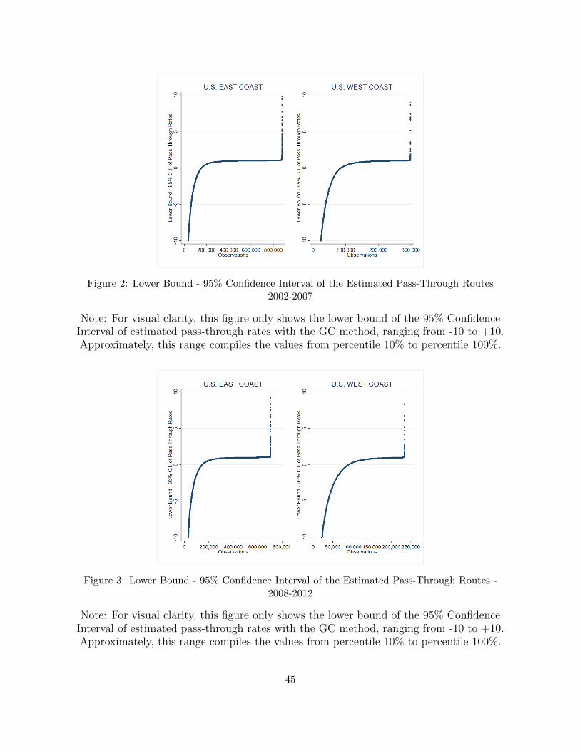
Figure 2: Lower Bound - 95% Confidence Interval of the Estimated Pass-Through Routes2002-2007
Note: For visual clarity, this figure only shows the lower bound of the 95% ConfidenceInterval of estimated pass-through rates with the GC method, ranging from -10 to +10.Approximately, this range compiles the values from percentile 10% to percentile 100%.
Figure 3: Lower Bound - 95% Confidence Interval of the Estimated Pass-Through Routes -2008-2012
Note: For visual clarity, this figure only shows the lower bound of the 95% ConfidenceInterval of estimated pass-through rates with the GC method, ranging from -10 to +10.Approximately, this range compiles the values from percentile 10% to percentile 100%.
45

Figure 4: Lower Bound - 95% Confidence Interval of the Estimated Pass-Through Routes -2013-2017
Note: For visual clarity, this figure only shows the lower bound of the 95% ConfidenceInterval of estimated pass-through rates with the GC method, ranging from -10 to +10.Approximately, this range compiles the values from percentile 10% to percentile 100%.
46

Figure 5: U.S. East Coast: Short Run Pass-Through Rate vs. Shipping Distance
Note: these figures show non-parametric predictions for the short-run pass through rates,assuming an Epanechnikov kernel with bandwidth optimally defined by cross-validation.
Figure 6: U.S. West Coast: Short Run Pass-Through Rate vs. Shipping Distance
Note: these figures show non-parametric predictions for the short-run pass through rates,assuming an Epanechnikov kernel with bandwidth optimally defined by cross-validation.
47

Figure 7: U.S. East Coast: Short Run Pass-Through Rate vs. Origin Country GDP per capita
Note: these figures show non-parametric predictions for the short-run pass through rates,assuming an Epanechnikov kernel with bandwidth optimally defined by cross-validation.
Figure 8: U.S. West Coast: Short Run Pass-Through Rate vs. Origin Country GDP per capita
Note: these figures show non-parametric predictions for the short-run pass through rates,assuming an Epanechnikov kernel with bandwidth optimally defined by cross-validation.
48

Figure 9: Composition of Ad-Valorem % Maritime Shipping Freights
49

Appendixes
A Mathematical Derivations
Derivation Eq. (3)To decompose the short-run pass-through rate ρkr , equation (2) shows that the first-order conditionof carriers’ maximization problem is given by:
f `,kr = c`(χkr )−∂fkr∂Qkr
∂Qkr∂qk`,r
qk`,r (A.1)
Now, defining a standard conduct parameter θkr = ∂Qkr∂qkl,r
, and differentiating this expression with
respect to the shipping cost c(χkr ), the short-run pass-through rate ρkr is equal to:
ρkr =∂fkr∂c(χkr )
=
[1 +
1 + Ekr (fkr )
φkr
]−1(A.2)
Derivation Eq. (5)To derive the optimal pricing-rule for maritime shipping carriers, I know from equation (2) thatthe first-order condition of carriers maximization problem is given by:
f `,kr = c`(χkr )−∂fkr∂Qkr
∂Qkr∂qk`,r
qk`,r (A.3)
Writing the shipping freight rate f `,kr as the wedge between the price of product k in the origin P koand in the destination country P kd yields:
P kd = P ko + c`(χkr )−∂(P kd − P ko )
∂Qkr
∂Qkr∂qkl,r
qkl,r (A.4)
Now, defining and substituting a standard conduct parameter θkr = ∂Qkr∂qkl,r
, and invoking the as-
sumption that demand for importing product k in market d does not affect the price in the originmarket o, yields
P kd = P ko + c`(χkr )−∂P kd∂Qkr
θkrQkl,r
Lkl,r
= P ko + c`(χkr )−∂P kd∂Qkr
Qkrφkr
(A.5)
In parallel, differentiating the assumed Bulow and Pfleiderer (1983) inverse demand for maritime
50

shipping services with respect to the aggregate quantity of product k, that it is shipped per router, yields:
∂P kod∂Qkr
= −bkodδkodQkrδkod−1 (A.6)
which given the structure on this demand function is equivalent to:
∂P kod∂Qkr
Qkr = −δkod(akod − P kod) (A.7)
Then, substituting this expression into the optimal pricing-rule defined above yields:
P kod = P ko + c`(χkr ) +δkod(a
kod − P kod)φkr
(A.8)
Finally, substituting the definition of the short-run pass-through rate, ρkr =[1+
δkodφkod
]−1and writing
the spatial price gap, as the shipping freight rate, f `,kr = P kd = P ko , yields:
f `,kr = ρkrc`(χkr ) + (1− ρkr )(akod − P ko ) (A.9)
Derivation Eq. (7)To derive this expression, I substitute in expression (6) the additive structural forms for c`(χkr ) andakod similar to Atkin and Donaldson (2015), one for each shipping route r in each shipping U.S.coast c, yielding:
P k,cod = ρkrPk,co + ρkrc
`(χk,cr ) + (1− ρkr )ak,cod
= ρkrPk,co + ρkr
[∑d
(βk,c1,r + βk,c2,r t+ ξk,cr )]
+ (1− ρkr )[∑
d
(αk,c1,od + αk,c2,odt+ υk,cod )]
(A.10)
Rearranging terms and approximating ρkr with ρk,co yields:
P k,cod = ρk,co P ko +∑d
([ρkrβ
k1,r + (1− ρk,co )αk1,d
]+[ρkrβ
k2,r + (1− ρk,co )αk2,d
]t+
[ρkrξ
kr + (1− ρk,co )υkod
])
(A.11)
which can be written as:
P k,cod = ρk,co P k,oo +∑d
(γk,cod + γk,cod t) + εkod (A.12)
51

Derivation Eq. (12)To derive the expression for calculating maritime shipping mark-ups, I know that the optimalpricing-rule can be written as:
f `,k,cr = ρk,co P k,coT `(χk,cr ) + (1− ρk,co )(ak,cod − P
k,co ) (A.13)
Subtracting the shipping costs function in both sides yields:
f `,k,cr − P k,coT `(χk,cr ) = (1− ρk,co )(ak,cod − P
k,co
T `(χk,cr )− P k,co ) (A.14)
Finally, calculating the ratio of this expression to the shipping freight rates yields:
µ`,k,cr =(1− ρk,co )(ak,cod − (1 +
T `(χk,cr ))P k,co )
P k,cod − Pk,co
(A.15)
Derivation Eq. (13)To derive this equivalent expression for calculating maritime shipping mark-ups, I know that themark-ups are given as follows from expression (12):
µ`,k,cr =(1− ρk,co )(ak,cod − (1 +
T `(χk,cr ))P k,co )
P k,cod − Pk,co
(A.16)
Now, substituting the spatial price gap definition of the shipping freight rates, the mark-ups canbe written as:
µ`,k,cr =
(1− ρk,co
ρk,co
)(ak,cod − P
k,cd
P k,cod − Pk,co
)(A.17)
In parallel, calculating the elasticity of the shipping inverse demand yields:
ηk,cr = −
(ak,cod − P
k,cod
P k,cod
)δk,cr (A.18)
Finally, solving for the difference between ak,cod and P k,cod and substituting in the expression derivedabove for the mark-ups, yields:
µ`,k,cr = −
(1− ρk,co
ρk,co
)(ηk,cr
δk,cr
)(P k,cod
P k,cod − Pk,co
)(A.19)
52

Derivation Eq. (14)To derive this expression, I differentiate the structural specification of the maritime shipping mark-ups defined in expression (12) with respect the short-run pass-through rate.
∂µ`,k,cr
∂ρk,co= (1− ρk,co )
[−ak,cod −
T `(χk,cr )P k,co − P kco
(P k,cod − Pk,co )2
]∂P k,cod
∂ρk,co−
[ak,cod −
T `(χk,cr )P k,co − P k,co
P k,cod − Pk,co
](A.20)
Substituting the expression derived above for the maritime shipping mark-ups yields:
∂µ`,k,cr
∂ρk,co= −µ`,k,cr
[∂P k,cod
∂ρk,co
1
(P k,cod − Pk,co )
+1
1− ρk,co
](A.21)
Differentiating expression (13) specified in unit prices, with respect the short-run pass-throughrate, and rearranging terms yields:
∂µ`,k,cr
∂ρk,co=µ`,k,cr (1− µ`,k,cr )
ρk,co − 1(A.22)
which permits to define the elasticity of the maritime shipping mark-ups to the short-run pass-through rates (ε`,k,cr,(ρ,µ)) as:
ε`,k,cr,(ρ,µ) =∂µ`,k,cr
∂ρk,co
ρk,co
µ`,k,cr
=
(ρk,co − 1
ρk,co
)−1(1− µ`,k,cr ) (A.23)
53

B Data Description
As noted above, I use in this paper data from the U.S. Merchandise Imports for the period 2002-2017. Specifically, I use a data sample which I built exclusively for U.S. imports shipped by sea. Todo so, I started off working with the complete U.S. Merchandise Imports database for the period2002-2017 pulled from the U.S. Census Bureau, which compiles annual U.S. imports by HS10-digit product k, origin country o, U.S. customs district of arrival d and year t. Then, I applied thefollowing step-wise procedure, which generated the final database that I used for all estimationsin this paper.
First, I kept only those import flows shipped by sea. To do so, I dropped all observations forwhich imports value and/or imports weight moved by sea were equal to zero. Second, I kept inthe database those import flows that certainly were shipped to the U.S. by sea. For this purpose,I trimmed all import flows that entered into the U.S. via any inland customs district followingHummels and Schaur (2013). These imports flows might have originally arrived to the U.S. by seabut presumably were only recorded in these inland regions. This is an issue, given that they musthave arrived to these regions via others mode of transportation (e.g. air or ground) for which Iignore the transportation costs information. So, I excluded these shipments to abstract the estima-tions from this potential noise. Third, I dropped from the database all import flows coming fromCanada and Mexico. Those flows might not be reliable for estimating the maritime shipping costsand maritime shipping mark-ups from shipments coming from these countries, given that a largeportion of these flows is moved by ground. Forth, I trimmed all imports flows within each HS6-digit product group in a year t imported from a particular origin country o with either unit pricesor ad-valorem freight charges below the 1st percentile or above the 99th percentile. The rationale isthat I develop this paper at the HS6-digit product k level. Thus, to avoid the potential problem ofcombining imports flows from products within the same HS6-digit product group and importedfrom the same country with different shipping characteristics, I trimmed these observations fol-lowing consistently to Hummels and Schaur (2013). Fifth, I dropped all import flows for which itis unknown the SITC code, using as reference the annual U.S. Census Concordance. This code iskey for determining whether a product is homogeneous or differentiated according to the Rauch(1999) product classification. Thus, it provides a good idea of the shipping technology used forshipping a products. Sixth, I merged the conservative Rauch (1999) product classification, trim-ming all observations for which it is unknown the correlation in the U.S. database. As explainedabove, I used this classification to infer the most presumable technology for shipping the products(i.e. bulk or liner shipping). Finally, I dropped all HS6-digit product codes pooling products con-sidered homogeneous and other differentiated at the HS10 digit product level. I assumed this is aclear signal of heterogeneity within a HS6 digit product group.
Thus, the database I ended up using in this paper considers approximately 91% to 94% of thetotal value of the U.S. imports moved by sea over the period 2002-2017. Each observation inthis database compiles information disaggregated by HS6-digit product k, origin country o, U.S.customs district of arrival d and year t for (1) the imports’ FOB value (in current U.S.$), (2) theimports’ CIF value (in current U.S.$), (3) imported quantities (in kg.), and (4) the cost of insurancesand freight.
54

The maritime shipping distance I use in all estimations is calculated using the World Cities Databaseretrieved from https://simplemaps.com/data/world-cities. This database provides the GPScoordinates (i.e. longitude and latitude) from all cities worldwide, relying on gathered data fromNGIA, US Geographical Survey, US Census Bureau and NASA. So, to calculate the shipping dis-tance for all shipping routes in the US imports database, I applied the great-circle distance formulato the GPS coordinates of each route. A problem that surged was how to merge this databaseof shipping distances to the U.S. imports database. As explained, the U.S. imports database re-ports each import flow by origin country o and U.S. customs district of arrival d. In contrast, thedatabase built for the distances was at the city level in each origin country to each U.S. customsdistrict. Thus, to circumvent this problem, I adjusted the database of distances as follows. First, Icalculated a weighted average distance from every origin country o to every U.S. customs districtd, using (1) all shipping distances previously calculated from each city in a particular origin coun-try o to each U.S. customs district d; and (2) the population shares of each city in an origin countryo as shares for this calculation. Exceptionally, I calculated these distances as a simple average inthose cases in which it lacked these population shares. Second, I considered some geographicalrestrictions in these calculations. For the sake of simplicity, I assumed that all shipments comingto the U.S. East coast from Europe and Africa occurs point-to-point, whereas those coming fromAsia and Australia arrive via the Panama Canal. Similarly, I assume that all shipments comingto the U.S. West coast from Asia and Australia occurs point-to-point, while those coming fromEuropa and Africa arrive via the Panama Canal. In addition, I assumed that all shipments com-ing from Latin America are point-to point or via the Panama Canal, depending on the ocean overeach country has located its main maritime port. To define these regions, I used the World Bankgeographical classification. That is, Europe compiles all countries in the World Bank’s regionsEurope & Central Asia; Africa compiles all countries in regions Middle East & North Africa andSub-Saharan Africa; Asia compiles all countries in regions East Asia & Pacific and South Asia; andLatin America compiles all countries in region Latin America and the Caribbean.
Other sources used to build this database are CEPII and BACI. From CEPII, I pulled the GDPper capita and from BACI the data to calculate the Revealed Comparative Advantage (RCA) (as astandard Balassa Index) and the World Export Supply (WES) (Balassa (1965) and Hummels et al.(2014)). I also employ the U.S. Tariffs database from the USITC. Additionally, I used the sub-stitution elasticities calculated by Soderbery (2015), using the hybrid Feenstra (1994)/Broda andWeinstein (2006) methodology. Finally, I deflated all figures with the annual average of the U.S.Consumer Price Index (CPI), setting as the basis year 2017.
55

C Analysis of the Data
Table C1: Value of U.S. Imports (U.S. $billions) (constant prices of 2017)
U.S. East Coast U.S. West Coast
2002-2007 2002-2007
OLS % 2SLS % GC % OLS % 2SLS % GC %
Included in the analysis† 1,567 97.8% 1,554 96.9% 1,592 99.3% 1,450 96.1% 1,444 95.7% 1,501 99.5%Excluded from the analysis‡ 36 2.3% 49 3.1% 11 0.7% 59 3.9% 65 4.3% 8 0.5%
TOTAL 1,603 100.0% 1,603 100.0% 1,603 100.0% 1,509 100.0% 1,509 100.0% 1,509 100.0%
2008-2012 2008-2012
OLS % 2SLS % GC % OLS % 2SLS % GC %
Included in the analysis† 1,368 98.6% 1,348 97.2% 1,379 99.4% 1,282 98.9% 1,275 98.4% 1,290 99.5%Excluded from the analysis‡ 19 1.4% 39 2.8% 8 0.6% 13 1.0% 21 1.6% 5 0.4%
TOTAL 1,387 100.0% 1,387 100.0% 1,387 100.0% 1,296 100.0% 1,296 100.0% 1,296 100.0%
2013-2017 2013-2017
OLS % 2SLS % GC % OLS % 2SLS % GC %
Included in the analysis† 1,692 98.5% 1,675 97.5% 1,711 99.6% 1,379 98.9% 1,357 97.3% 1,390 99.6%Excluded from the analysis‡ 26 1.5% 43 2.5% 7 0.4% 17 1.2% 38 2.7% 5 0.4%
TOTAL 1,718 100.0% 1,718 100.0% 1,718 100.0% 1,395 100.0% 1,395 100.0% 1,395 100.0%
†: all pairs product k - origin country o for which it is feasible estimating a short-run pass-through rate (i.e. ρ >0).‡: all pairs (product k - origin country o) for which it is not possible or is unfeasible estimating a short-run pass-through rate(i.e. ρ ≤0).
56

Table C2: HS6-digit Products in Sampling Data
U.S. East Coast U.S. West Coast
2002-2007 2002-2007
OLS % 2SLS % GC % OLS % 2SLS % GC %
Included in the analysis† 2,942 89.9% 2,910 88.9% 3,141 95.9% 2,820 87.5% 2,785 86.4% 2,967 92.0%Excluded from the analysis‡ 332 10.1% 364 11.1% 133 4.1% 404 12.5% 439 13.6% 257 8.0%
TOTAL 3,274 100.0% 3,274 100.0% 3,274 100.0% 3,224 100.0% 3,224 100.0% 3,224 100.0%
2008-2012 2008-2012
OLS % 2SLS % GC % OLS % 2SLS % GC %
Included in the analysis† 2,823 93.6% 2,783 92.3% 2,903 96.3% 2,722 91.7% 2,678 90.2% 2,782 93.7%Excluded from the analysis‡ 192 6.4% 232 7.7% 112 3.7% 246 8.3% 290 9.8% 186 6.3%
TOTAL 3,015 100.0% 3,015 100.0% 3,015 100.0% 2,968 100.0% 2,968 100.0% 2,968 100.0%
2013-2017 2013-2017
OLS % 2SLS % GC % OLS % 2SLS % GC %
Included in the analysis† 2,827 93.1% 2,797 92.1% 2,935 96.6% 2,730 91.2% 2,698 90.2% 2,819 94.2%Excluded from the analysis‡ 211 6.9% 241 7.9% 103 3.4% 262 8.8% 294 9.8% 173 5.8%
TOTAL 3,038 100.0% 3,038 100.0% 3,038 100.0% 2,992 100.0% 2,992 100.0% 2,992 100.0%
†: all pairs product k - origin country o for which it is feasible estimating a short-run pass-through rate (i.e. ρ >0).‡: all pairs (product k - origin country o) for which it is not possible or is unfeasible estimating a short-run pass-through rate(i.e. ρ ≤0).
57

Table C3: Countries in Sampling Data
U.S. East Coast U.S. West Coast
2002-2007 2002-2007
OLS % 2SLS % GC % OLS % 2SLS % GC %
Included in the analysis† 192 84.6% 171 75.3% 205 90.3% 151 69.9% 138 63.9% 161 74.5%Excluded from the analysis‡ 35 15.4% 56 24.7% 22 9.7% 65 30.1% 78 36.1% 55 25.5%
TOTAL 227 100.0% 227 100.0% 227 100.0% 216 100.0% 216 100.0% 216 100.0%
2008-2012 2008-2012
OLS % 2SLS % GC % OLS % 2SLS % GC %
Included in the analysis† 180 79.6% 158 69.9% 196 86.7% 146 69.5% 127 60.5% 154 73.3%Excluded from the analysis‡ 46 20.4% 68 30.1% 30 13.3% 64 30.5% 83 39.5% 56 26.7%
TOTAL 226 100.0% 226 100.0% 226 100.0% 210 100.0% 210 100.0% 210 100.0%
2013-2017 2013-2017
OLS % 2SLS % GC % OLS % 2SLS % GC %
Included in the analysis† 188 82.1% 161 70.3% 202 88.2% 151 69.3% 132 60.6% 156 71.6%Excluded from the analysis‡ 41 17.9% 68 29.7% 27 11.8% 67 30.7% 86 39.4% 62 28.4%
TOTAL 229 100.0% 229 100.0% 229 100.0% 218 100.0% 218 100.0% 218 100.0%
†: all pairs product k - origin country o for which it is feasible estimating a short-run pass-through rate (i.e. ρ >0).‡: all pairs (product k - origin country o) for which it is not possible or is unfeasible estimating a short-run pass-through rate(i.e. ρ ≤0).
58

D Robustness Exercises
Table D1: Summary Statistics - Short Run Pass Through-Rate ρ(HS6 digit-code vs HS10 digit-code, Gaussian Copula Estimates)
U.S. East Coast
2002-2007 2013-2017
HS6 HS10 HS6 HS10
(1) (2) (5) (6)
Mean 1.42 1.56 1.16 1.38Median 1.01 1.01 1.01 1.01Std Deviation 31.98 53.42 9.78 31.79Percentile 1% 0.43 0.39 0.46 0.40Percentile 99% 2.71 2.98 2.47 2.71Number Obs. 55,212 107,719 52,277 103,990
U.S. West Coast
2002-2007 2013-2017
HS6 HS10 HS6 HS10
(1) (2) (5) (6)
Mean 1.11 1.36 1.13 1.13Median 1.01 1.01 1.00 1.00Std Deviation 3.14 47.99 8.61 8.27Percentile 1% 0.46 0.43 0.46 0.44Percentile 99% 2.30 2.36 2.14 2.36Number Obs. 31,823 60,813 28,819 55,637
59

Table D2: Median Maritime Shipping Mark-up - % of Maritime Shipping Freight Freight(HS6 digit-code vs HS10 digit-code, Gaussian Copula Estimates)
U.S. East Coast U.S. West Coast
2002-2007 2013-2017 2002-2007 2013-2017
(1) (2) (3) (4)
HS6 digit-code 43.4 34.1 34.2 32.7HS10 digit-code 38.0 28.2 37.9 30.1
60

Figure D1: Comparison Estimated Short-Run Pass-Through Rates at HS6 vs at HS10 - Period2002-2007
Note: For visual purposes, this figure excludes short-run pass-through rates higher than 30.Those observations account for less than 1% of the total.
61

Figure D2: Comparison Estimated Short-Run Pass-Through Rates at HS6 vs at HS10 - Period2013-2017
Note: For visual purposes, this figure excludes short-run pass-through rates higher than 30.Those observations account for less than 1% of the total.
62

Table D3: Summary Statistics - Short-Run Pass-Through Rates(SITC Rev. 2 versus SITC Rev. 4 to classify U.S. Imports)
U.S. East Coast
2002-2007 2008-2012 2013-2017
HS10 SITC Rev. 2 HS10 SITC Rev. 4 HS10 SITC Rev. 2 HS10 SITC Rev. 4 HS10 SITC Rev. 2 HS10 SITC Rev. 4
(1) (2) (3) (4) (5) (6)
Mean 1.56 1.60 1.62 1.64 1.38 1.37Median 1.01 1.01 1.01 1.01 1.01 1.01Std Deviation 53.42 55.29 117.54 119.59 31.79 32.04Percentile 1% 0.39 0.39 0.41 0.42 0.40 0.41Percentile 99% 2.98 2.97 2.71 2.69 2.71 2.67Number Obs. 107,718 103,474 93,031 89,867 103,990 100,707
U.S. West Coast
2002-2007 2008-2012 2013-2017
HS10 SITC Rev. 2 HS10 SITC Rev. 4 HS10 SITC Rev. 2 HS10 SITC Rev. 4 HS10 SITC Rev. 2 HS10 SITC Rev. 4
(1) (2) (3) (4) (5) (6)
Mean 1.36 1.37 1.21 1.22 1.13 1.13Median 1.01 1.01 1.00 1.00 1.00 1.00Std Deviation 47.99 48.92 28.75 29.22 8.27 8.38Percentile 1% 0.43 0.44 0.43 0.44 0.44 0.45Percentile 99% 2.36 2.38 2.27 2.24 2.36 2.35Number Obs. 60,812 58,513 51,617 49,959 55,637 53,956
63

Table D4: Median Maritime Shipping Mark-up(SITC Rev. 2 versus SITC Rev. 4 to classify U.S. Imports)
U.S. East Coast U.S. West Coast
2002-2007 2008-2012 2013-2017 2002-2007 2008-2012 2013-2017
(1) (2) (3) (4) (5) (6)
HS10 - SITC Rev. 2 38.0 29.2 28.2 37.9 -60.2 30.1HS10 - SITC Rev. 4 38.7 29.0 28.8 37.9 -45.6 30.3
64