Tracking Vehicular Speed Variations by Warping

Mobile Phone Signal Strengths

Gayathri Chandrasekaran∗, Tam Vu∗ Alexander Varshavsky†, Marco Gruteser∗,

Richard P. Martin∗, Jie Yang‡, Yingying Chen‡

∗ WINLAB, Rutgers University † AT&T Labs ‡ Stevens Institute of Technology

North Brunswick, NJ 08902 Florham Park, NJ 07932 Hoboken, NJ 07030

{chandrga, tamvu, gruteser, rmartin} {varshavsky} {jyang, yingying.chen}@winlab.rutgers.edu @research.att.com @stevens.edu

Abstract—In this paper, we consider the problem of trackingfine-grained speeds variations of vehicles using signal strengthtraces from GSM enabled phones. Existing speed estimationtechniques using mobile phone signals can provide longer-termspeed averages but cannot track short-term speed variations.Understanding short-term speed variations, however, is impor-tant in a variety of traffic engineering applications—for example,it may help distinguish slow speeds due to traffic lights fromtraffic congestion when collecting real time traffic information.Using mobile phones in such applications is particularly attractivebecause it can be readily obtained from a large number ofvehicles.

Our approach is founded on the observation that the large-scale path loss and shadow fading components of signal strengthreadings (signal profile) obtained from the mobile phone on anygiven road segment appear similar over multiple trips along thesame road segment except for distortions along the time axisdue to speed variations. We therefore propose a speed trackingtechnique that uses a Derivative Dynamic TimeWarping (DDTW)algorithm to realign a given signal profile with a known trainingprofile from the same road. The speed tracking technique thentranslates the warping path (i.e., the degree of stretching andcompressing needed for alignment) into an estimated speed trace.Using 6.4 hours of GSM signal strength traces collected from avehicle, we show that our algorithm can estimate vehicular speedwith a median error of ± 5mph compared to using a GPS andcan capture significant speed variations on road segments witha precision of 68% and a recall of 84%.

I. INTRODUCTION

This paper considers the problem of estimating fine-grained

speed and detecting temporary speed variations of a vehicle

from cellular handset signals. More fine-grained speed traces

could benefit a number of transportation applications. For ex-

ample, fine-grained speed trace could improve estimating and

pinpointing traffic congestion, particularly on arterial roads

with traffic signals. Since fine-grained speed traces reveal

where on a road segment vehicles slow down, it becomes

easier to distinguish speed variations due to congestion from

slowdowns due to red traffic lights. Fine-grained speed traces

also reveal whether traffic is flowing slow but smoothly or

in a stop-and-go fashion. It can also show where frequent

lane changes occur that cause traffic shock waves. These

factors have a significant effect on accident rates and gasoline

consumption, and would therefore be important to monitor

on a larger scale. Techniques to determine vehicle speed

from cell phone signals are particularly useful because they

do not incur the high infrastructure costs of traffic cameras

or loop detectors embedded into the roadway [9], [8], [13].

While fine-grained speed traces can also be obtained through

networked in-vehicle GPS devices, cell phone signals can

readily be collected from a much larger number of vehicles.

Collecting cell phone signal strength readings at the base

station imposes no energy overhead, since the cell phones that

are active on call periodically transmit Network Measurement

Reports (NMR) containing signal strength readings to the base

station. Existing speed estimation techniques from cell phone

communications are limited to estimating average speeds over

road segments. One approach derives speed from the time

between two handoffs [24], [12]. In our own prior work [6],

we have also shown how average speeds can be estimated by

matching a cell phone’s signal strength trace against a known

trace from this road segment. While these solutions can cover

most of the arterial roads, the average speed estimates are

typically over road segments of about 100m and cannot track

vehicle’s exact speed variations.

Our Approach. In this paper, we propose a technique based

on a Derivative Dynamic Time Warping (DDTW) algorithm

that aligns a received signal strength (RSS) trace from a

moving cell phone handset with a reference trace for a

given road segment to estimate the speed of the moving cell

phone. The technique relies on the observation that large scale

path loss and dominant shadow fading effects usually remain

quite constant at the same location. To illustrate this insight,

Fig. 1 plots the instantaneous speed and RSS trace from the

associated cell tower for two vehicle trips along the same

stretch of a road. The vehicle drove roughly at the same speed

during the first 150 seconds of both trips, but then it slowed

down in the first trip and sped up in the second.1 The graph

shows how the RSS traces remain similar over the first part

of the trace, where the vehicle traveled at the same speed, and

1The car traveled the same distance in both cases and stopped at the samephysical location. However, due to the speed difference, the first trip tookabout 300 seconds while the second only lasted 200 seconds.

2011 IEEE International Conference on Pervasive Computing and Communications (PerCom), Seattle (March 21-25, 2011)

978-1-4244-9529-0/11/$26.00 ©2011 IEEE 213

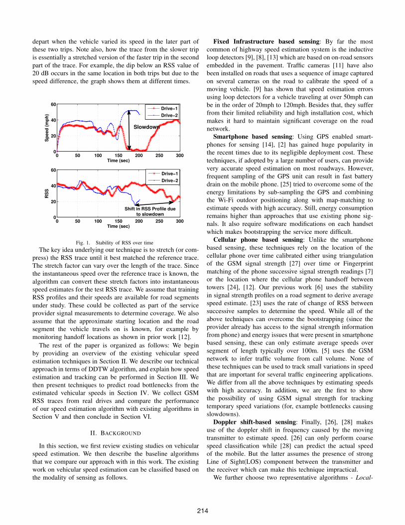
depart when the vehicle varied its speed in the later part of

these two trips. Note also, how the trace from the slower trip

is essentially a stretched version of the faster trip in the second

part of the trace. For example, the dip below an RSS value of

20 dB occurs in the same location in both trips but due to the

speed difference, the graph shows them at different times.

0 50 100 150 200 250 3000

20

40

60

Time (sec)

Sp

ee

d (

mp

h)

Drive−1

Drive−2

0 50 100 150 200 250 3000

20

40

60

Time (sec)

RS

S

Drive−1

Drive−2

Slowdown

Shift in RSS Profile dueto slowdown

Fig. 1. Stability of RSS over time

The key idea underlying our technique is to stretch (or com-

press) the RSS trace until it best matched the reference trace.

The stretch factor can vary over the length of the trace. Since

the instantaneous speed over the reference trace is known, the

algorithm can convert these stretch factors into instantaneous

speed estimates for the test RSS trace. We assume that training

RSS profiles and their speeds are available for road segments

under study. These could be collected as part of the service

provider signal measurements to determine coverage. We also

assume that the approximate starting location and the road

segment the vehicle travels on is known, for example by

monitoring handoff locations as shown in prior work [12].

The rest of the paper is organized as follows: We begin

by providing an overview of the existing vehicular speed

estimation techniques in Section II. We describe our technical

approach in terms of DDTW algorithm, and explain how speed

estimation and tracking can be performed in Section III. We

then present techniques to predict road bottlenecks from the

estimated vehicular speeds in Section IV. We collect GSM

RSS traces from real drives and compare the performance

of our speed estimation algorithm with existing algorithms in

Section V and then conclude in Section VI.

II. BACKGROUND

In this section, we first review existing studies on vehicular

speed estimation. We then describe the baseline algorithms

that we compare our approach with in this work. The existing

work on vehicular speed estimation can be classified based on

the modality of sensing as follows.

Fixed Infrastructure based sensing: By far the most

common of highway speed estimation system is the inductive

loop detectors [9], [8], [13] which are based on on-road sensors

embedded in the pavement. Traffic cameras [11] have also

been installed on roads that uses a sequence of image captured

on several cameras on the road to calibrate the speed of a

moving vehicle. [9] has shown that speed estimation errors

using loop detectors for a vehicle traveling at over 50mph can

be in the order of 20mph to 120mph. Besides that, they suffer

from their limited reliability and high installation cost, which

makes it hard to maintain significant coverage on the road

network.

Smartphone based sensing: Using GPS enabled smart-

phones for sensing [14], [2] has gained huge popularity in

the recent times due to its negligible deployment cost. These

techniques, if adopted by a large number of users, can provide

very accurate speed estimation on most roadways. However,

frequent sampling of the GPS unit can result in fast battery

drain on the mobile phone. [25] tried to overcome some of the

energy limitations by sub-sampling the GPS and combining

the Wi-Fi outdoor positioning along with map-matching to

estimate speeds with high accuracy. Still, energy consumption

remains higher than approaches that use existing phone sig-

nals. It also require software modifications on each handset

which makes bootstrapping the service more difficult.

Cellular phone based sensing: Unlike the smartphone

based sensing, these techniques rely on the location of the

cellular phone over time calibrated either using triangulation

of the GSM signal strength [27] over time or Fingerprint

matching of the phone successive signal strength readings [7]

or the location where the cellular phone handsoff between

towers [24], [12]. Our previous work [6] uses the stability

in signal strength profiles on a road segment to derive average

speed estimate. [23] uses the rate of change of RSS between

successive samples to determine the speed. While all of the

above techniques can overcome the bootstrapping (since the

provider already has access to the signal strength information

from phone) and energy issues that were present in smartphone

based sensing, these can only estimate average speeds over

segment of length typically over 100m. [5] uses the GSM

network to infer traffic volume from call volume. None of

these techniques can be used to track small variations in speed

that are important for several traffic engineering applications.

We differ from all the above techniques by estimating speeds

with high accuracy. In addition, we are the first to show

the possibility of using GSM signal strength for tracking

temporary speed variations (for, example bottlenecks causing

slowdowns).

Doppler shift-based sensing: Finally, [26], [28] makes

use of the doppler shift in frequency caused by the moving

transmitter to estimate speed. [26] can only perform coarse

speed classification while [28] can predict the actual speed

of the mobile. But the latter assumes the presence of strong

Line of Sight(LOS) component between the transmitter and

the receiver which can make this technique impractical.

We further choose two representative algorithms - Local-

214

ization Algorithm and Normalized Euclidean Distance Algo-

rithm, that have previously been used for tracking vehicular

speed and detecting bottlenecks in road segments, as base-

line approaches for comparing our algorithm with. Note that

the performance of the localization algorithms for tracking

speed variations are similar to our prior speed estimation

algorithm [6]. We therefore only include the more general and

better known localization algorithm as a baseline algorithm.

Localization Algorithm: This method as implemented by

several commercial products [1], [21] estimates the speed of a

mobile phone between two points by estimating the phone’s lo-

cations at the two points, calculating the distance the phone has

traveled and dividing it by the time traveled. In this paper, we

use the fingerprinting [19] algorithm for determining phone’s

location. The algorithm uses the RSS fingerprints obtained

from 7 neighboring towers at different known locations as the

training. When an RSS fingerprint is obtained from a mobile

at an unknown location, the algorithm estimates the euclidean

distance in signal space between this obtained fingerprint and

all the training fingerprints and determines the location to be

the location of the training fingerprint that yields the minimum

euclidean distance.

Normalized Euclidean Distance Algorithm: This algo-

rithm detects speed changes during speed tracking, e.g.,

slowdowns, by calculating the normalized euclidean distance

between consecutive GSM measurements and declaring a

slowdown when the distance falls beyond a certain threshold.

The normalized Euclidean distance between two RSS mea-

surements A and B, having n common cell towers is defined

as:

√

(a1 − b1)2 + (a2 − b2)2 + ....+ (an − bn)2/n (1)

Note that Euclidean distance between successive samples

from a mobile phone is directly proportional to the distance

the phone moves in physical space, which in turn depends on

how fast the phone moves. While we cannot derive an accurate

speed estimate from this relation, we can still predict regions

where there are slowdowns. We experimented with multiple

other metrics suggested in [23], but found the normalized

euclidean distance to work the best. Hence, we chose to use

this algorithm for comparison with our mechanism.

III. SPEED TRACKING

Our speed tracking technique has two components. First, the

Derivative Dynamic Time Warping Algorithm (DDTW) [16]

optimally aligns a given RSS profile collected from a vehi-

cle moving at unknown speeds with a training RSS profile

collected from a vehicle moving at known speeds. The ser-

vice providers often collect RSS information along with the

location and speed information on different road segments to

assess network coverage. These logs can serve as the training

RSS profile for our DDTW algorithm. Second, the speed

tracker uses the alignment produced by the DDTW algorithm

to estimate the unknown speed of the moving vehicle which

can in turn be used for estimating vehicular slowdowns.

A. Derivative Dynamic Time Warping Algorithm

To find the optimal alignment between sequences of signal

strength measurements for speed estimation, we apply two

sequences of signal strength measurements, one called the

training and the other called the testing, to the Dynamic

Time Warping (DTW) Algorithm. Dynamic Time Warping

is a classic dynamic programming algorithm which has

been widely used for optimal alignment of two time series

datasets and was particularly popular for applications like

speech processing[17], [22], data mining[18], [15], and gesture

recognition[10].

In particular, we use a variant of the DTW algorithm

called Derivative Dynamic Time Warping (DDTW) [16],

which exploits the same principle as DTW but for the input

data, where, instead of the time-series of RSS, we use the

time-series of derivative of RSS. As observed previously [16],

if the two RSS profiles varied only on the time axis and

not on the absolute values of RSS at any given location,

DTW would have been sufficient. But RSS in an outdoor

environment typically suffers varying amount of shadow

fading under different environmental conditions which also

alters its absolute value in any given location. DDTW can

overcome this difference in the y-axis by working with

derivatives of RSS where only the slope of RSS matters and

not the absolute values. For example, if A = (a1, a2, ...aM )is a time series of RSS measurements collected over Mtime points, the input to DDTW is A′ = (a′1, a

′

2, ...a′

M ), thederivative of A which is defined as

a′i =(ai − ai−1) + (ai+1 − ai−1)/2

21 < i < M. (2)

Given two RSS profiles - A and B with lengths of M and

N samples respectively, DDTW constructs a distance matrix

d[M ×N ] which is defined as:

d(i, j) = (a′i − b′j)2 (3)

where a′i and b′j are the ith and jth elements of the derivative

of the RSS profiles A and B respectively. With this d[M×N ]as the input to the algorithm, DDTW returns a warping path

P = (p1, p2, ....pk) where pl = (x, y) ∈ [1 : M ] × [1 : N ]for l ∈ [1 : k] as shown in Figure 3. The warping path must

satisfy the following conditions:

1) Boundary Condition: p1 = (1, 1) and pk = (M,N).This ensures that the warping path always starts at (1, 1)and ends at (M,N).

2) Monotonicity Condition: If pk−1 = (c, d) and pk =(e, f), we have e − c ≥ 0 and f − d ≥ 0. The

monotonicity condition ensures that the matching always

progresses in the forward direction of time.

3) Global Constraints: Global constraints are constraints

that limit the region in which the warping path can

exist. In addition, global path constraints also guarantee

the existence of a path from (1, 1) to (M,N). Fig-

ure 3 illustrates the region for warping path generation.

The region enclosed within the parallelogram is the

region that corresponds to the global constraints. In

215

(i,j)(i,j-1)

(i-1,j)(i-1,j-1)

(a) Unconstrained

(i,j)(i,j-1)

(i-1,j-2) (i-1,j-2)

(i-1,j-1)

(i-1,j-1)

(b) Constrained, EMAX = 2

(i-1,j-k)

(i,j)

(i-k,j-1)

(i,j-1)(i,j-(k-1))

(i-1,j)

(i-(k-1),j)

(c) Constrained, EMAX = k

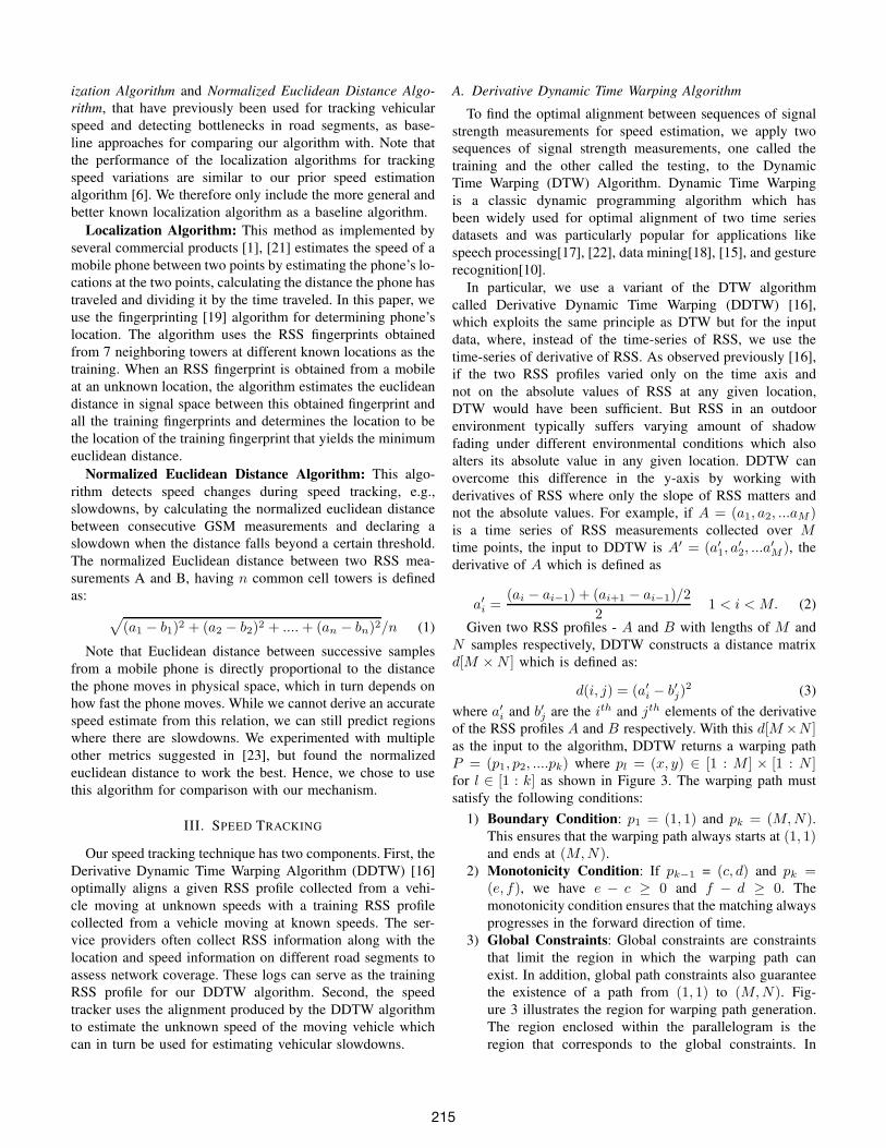
Fig. 2. DDTW local constraints that restrict the admissible paths to every location within the matrix:(a) C(i, j) = d(i, j) + min(C(i− 1, j − 1), C(i, j − 1), C(i− 1, j))(b) C(i, j) = d(i, j) + min(C(i − 1, j − 1), C(i− 1, j − 2) + d(i, j − 1), C(i− 2, j − 1) + d(i− 1, j))

(c) C(i, j) = min[

min1≤r≤EMAX

(

C(i− 1, j − r) +∑j

j1=j−(r−1)d(i, j1)

)

,min2≤r≤EMAX

(

C(i − r, j − 1) +∑i

i1=i−(r−1) d(i1, j))]

Figure 3, EMAX is defined as the maximum allow-

able expansion (or compression) in time axes of one

time series with respect to the other, and is chosen

to be max(2, ⌈max(M,N)/min(M,N)⌉). The ratio

⌈max(M,N)/min(M,N)⌉ defines the amount of ex-

pansion of one trace relative to the other. Accordingly,

the sides of the parallelogram are set to have slope values

of EMAX and 1/EMAX .

4) Local Constraints: Finally, Local constraints define the

set of admissible step-patterns. There are three types of

step progression: horizontal, vertical and diagonal. As

shown in Figure 2, different kinds of local constraints are

possible. For example, Figure 2(a) shows the most unre-

strictive step constraint where (i, j) can be reached from

one of its three neighbors (i−1, j−1), (i−1, j), (i, j−1).Whereas Figure 2(b) and 2(c) illustrate more constrained

progressions where a diagonal progression is forced for

every EMAX horizontal or vertical progressions.

To generate a warping path, DDTW constructs a cost matrix

C[M × N ] which represents the minimum cost to reach

any point (i, j) in the matrix from (1, 1) using a dynamic

programming formulation. For example, in Figure 2(a), (i, j)can be reached from one of its three neighbors, namely,

(i− 1, j− 1),(i− 1, j), and (i, j− 1), and the algorithm picks

the neighbor that has the minimum cost. This relation can be

shown as:

C(i, j) = d(i, j)+min(C(i−1, j−1), C(i, j−1), C(i−1, j)).(4)

However, using an unconstrained local constraint as shown

in 2(a) can lead to an undesirable effect called “singularities”

[16] where either one sample point in the testing is mapped to

a very large number of samples in training (unrestricted hori-

zontal progression) or many points in testing map to the same

point in training (unrestricted vertical progression). This effect

as observed previously[17] can be minimized by using a more

constrained topology for forward progression. In this work, we

thus take an approach of using the constrained DDTW with a

maximum expansion of EMAX . our local constraints resemble

the ones in Figure 2(b) and 2(c). For example, 2(b) forces

a diagonal progression before every horizontal or vertical

progression, whereas 2(c) allows up to (EMAX ) horizontal

or vertical progressions before forcing a diagonal progression.

For a complete description of local constraints, we refer the

readers to [17]. The local constraints that we use in this work

allow up to EMAX vertical or horizontal progressions before

forcing a diagonal progression and the cost matrix C(i, j)corresponding to this local constraint can be formulated as

C(i,j)=min[

min1≤r≤EMAX

(

C(i−1,j−r)+∑j

j1=j−(r−1)d(i,j1)

)

,

min2≤r≤EMAX (C(i−r,j−1)+∑i

i1=i−(r−1) C(i1,j))]

. (5)

Note that the optimal path to (i, j) depends only on the values

of (i′, j′) where i′ ≤ i and j′ ≤ j. From the cost matrix,

the algorithm derives a warping path P by back-tracking

the constructed cost matrix from (M,N) to (1, 1). While

backtracking, the path that the algorithm chooses from any

point (i, j) will be the (i′, j′) that resulted in optimal C(i, j).We will next explain how we use the warping path to estimate

the speed of the testing trace.

B. Estimating Vehicular Speed from DDTW’s warping path

The DDTW algorithm returns a warping path P between

the points (1, 1) to (M,N). This warping path defines the

optimal alignment between the training and the testing RSS

traces, i.e, it maps the RSS samples in the testing trace to the

RSS samples in the training trace. As explained in Section I,

there is a direct correlation between the speed of vehicle and

the overall shape of the RSS curve and the optimal mapping

of the RSS-curves can yield a speed estimate for the testing

trace relative to the training.

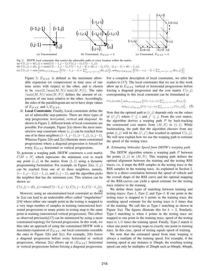
We define three types of matching between training and

testing traces: Type-1, Type-2, and Type-3. If one point in the

testing trace is mapped to k points in the training trace, the

resulting speed estimate for the testing trace is k times that

of the training. We call this as Type-1 matching as shown in

Figure 3(a). The figures illustrate this for k = 2. Similarly,

Type-3 matching is when k points in the testing trace are

mapped to one point in the training trace, speed of the testing

trace is 1/k times the training speed. Finally, Type-2 match is

when one point in testing maps to exactly one point in training

trace. In this case, speed of testing equals speed of training.

We note that the estimated speed from time warping is

always a multiple of the training speed. For example, if the

training speed at any instance is 20mph, the resulting testing

speed can only be multiples of 20mph such as 60mph, 40mph,

216

Test

ing

Training

Slope=1/EMAX

Slope=1/EMAX

Slope=EMAX

Type-1

Type-2

Test

ing

M × NSlope=EMAX

Type-3

(a) Cost Matrix C(M,N) and the warping path generation

Training

TestingSpeed of Testing = 2*Speed of Training

Speed of Testing = Speed of Training/2

(b) Optimal alignment of training and testing

20

10

40

Sp

ee

d (

mp

h) Training

Testing

0

30

(c) Estimated speed from a warping path

Fig. 3. Illustration of vehicular speed estimation from DDTW.

20mph or 10mph. Figure 3(b) plots the optimal alignment

between the training and the testing RSS traces obtained from

DDTW and illustrates the speed derivation procedure for the

testing trace. Figure 3(c) plots the estimated speeds for the

testing trace given a training trace with a constant speed of

20mph.

We observed that there are speed fluctuations in the esti-

mated speed. In order to remove these fluctuations, we apply

a moving window smoothing filter over the estimated speed

which averages the speed estimates within the entire window

to produce a single speed. The choice for the window size

should not be too large since this might smooth out all

variations leaving a very coarse speed estimate. Similarly,

having a very small window size may result in the overall

speed estimation to be highly fluctuating. We will evaluate

the length of the optimal smoothing window in Section V.

IV. SLOWDOWN DETECTION

In practice, most traffic engineering applications do not

require the instantaneous speeds of vehicles and are more

concerned about regions of bottlenecks. Such bottlenecks in

road networks can in turn be detected from vehicular speeds

by observing the regions where vehicles typically slowdown

or by observing the normalized euclidean distance where the

normalized euclidean distance between successive samples go

below a threshold. We will next provide a formal definition of

slowdown and describe the scheme for slowdown detection.

We define a slowdown as a sudden reduction in the speed of

a moving vehicle by more than τ mph to a value below µ mph.

The duration of the slowdown is the period of time the speed

remains below µ mph. A slowdown is detected by sequentially

scanning the input trace. The input trace can be the groundtruth

speed data derived from GPS readings, DDTW estimated

speed, speed estimate from the Localization algorithm, or the

Normalized Euclidean Distance from Normalized Euclidean

Distance algorithm. Our scheme identifies peaks and dips in

the input trace. A peak occurs in the input trace at any given

point when its first derivative (slope) at that point changes

from positive to negative. Similarly dips occur when the slope

changes from negative to positive. Our scheme initially assign

a very low value to the first detected peak and a very high value

to the first detected dip. As the scheme proceeds scanning the

trace, the peak value is adjusted to the highest observed peak.

Similarly, the dip value is adjusted to the lowest observed dip.

After every adjustment of the peak and the dip, if (peak−dip)> τ , and dip < µ, a slowdown is declared. The duration of thisslowdown is then the period of time the dip remains below µ.Finally, the peaks and dips are reset to the lowest and highest

values respectively and the scheme repeats until all slowdowns

are detected in the specific trace.

The main challenge in identifying slowdowns accurately lies

on the choice of τ and µ. We performed an empirical study

on 18 of our GPS traces that lasted for a total of 6.4 hours and

picked a threshold of 25mph for τ since most breaking events

involved slowing down the vehicle from 40-45mph speed limit

in arterial roads to a very slow speed of around 5-10mph. Our

choice for µ is 20mph because most residential regions have a

speed limit of 25mph or more and we do not want to classify

those residential regions as bottlenecks.

While a choice of 25mph and 20mph for τ and µ fits

the ground truth speed from GPS, these thresholds need not

be the same for the speeds estimated from either DDTW or

Localization. and the normalized euclidean distance estimated

by Normalized Euclidean Distance algorithm. For example, we

showed in Section III-B that the speed estimate from DDTW

at every instance is a multiple of the training speed which in

turn requires a moving window smoothing filter to be applied

over the estimated speed to get the speed estimate. However,

due to this smoothing, an actual speed change of 25mph in the

ground-truth speed may only correspond to a speed change of

15mph in the estimated speed.

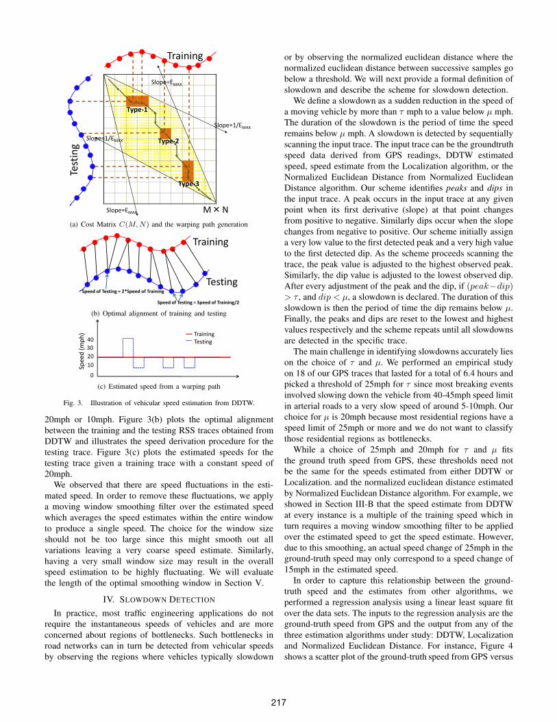
In order to capture this relationship between the ground-

truth speed and the estimates from other algorithms, we

performed a regression analysis using a linear least square fit

over the data sets. The inputs to the regression analysis are the

ground-truth speed from GPS and the output from any of the

three estimation algorithms under study: DDTW, Localization

and Normalized Euclidean Distance. For instance, Figure 4

shows a scatter plot of the ground-truth speed from GPS versus

217

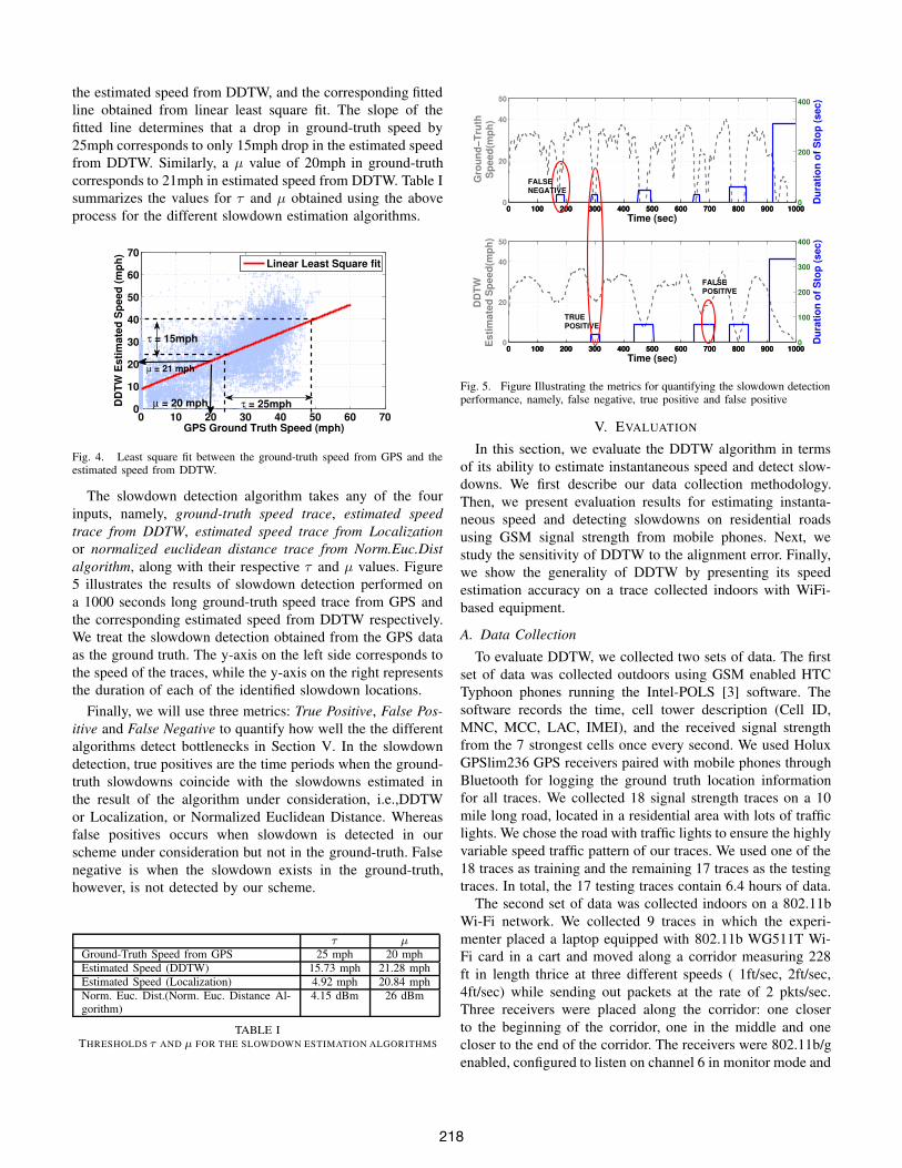
the estimated speed from DDTW, and the corresponding fitted

line obtained from linear least square fit. The slope of the

fitted line determines that a drop in ground-truth speed by

25mph corresponds to only 15mph drop in the estimated speed

from DDTW. Similarly, a µ value of 20mph in ground-truth

corresponds to 21mph in estimated speed from DDTW. Table I

summarizes the values for τ and µ obtained using the above

process for the different slowdown estimation algorithms.

0 10 20 30 40 50 60 700

10

20

30

40

50

60

70

GPS Ground Truth Speed (mph)

DD

TW

Es

tim

ate

d S

pe

ed

(m

ph

)

Linear Least Square fit

τ = 25mphµ = 20 mph

τ = 15mph

µ = 21 mph

Fig. 4. Least square fit between the ground-truth speed from GPS and theestimated speed from DDTW.

The slowdown detection algorithm takes any of the four

inputs, namely, ground-truth speed trace, estimated speed

trace from DDTW, estimated speed trace from Localization

or normalized euclidean distance trace from Norm.Euc.Dist

algorithm, along with their respective τ and µ values. Figure

5 illustrates the results of slowdown detection performed on

a 1000 seconds long ground-truth speed trace from GPS and

the corresponding estimated speed from DDTW respectively.

We treat the slowdown detection obtained from the GPS data

as the ground truth. The y-axis on the left side corresponds to

the speed of the traces, while the y-axis on the right represents

the duration of each of the identified slowdown locations.

Finally, we will use three metrics: True Positive, False Pos-

itive and False Negative to quantify how well the the different

algorithms detect bottlenecks in Section V. In the slowdown

detection, true positives are the time periods when the ground-

truth slowdowns coincide with the slowdowns estimated in

the result of the algorithm under consideration, i.e.,DDTW

or Localization, or Normalized Euclidean Distance. Whereas

false positives occurs when slowdown is detected in our

scheme under consideration but not in the ground-truth. False

negative is when the slowdown exists in the ground-truth,

however, is not detected by our scheme.

τ µGround-Truth Speed from GPS 25 mph 20 mph

Estimated Speed (DDTW) 15.73 mph 21.28 mph

Estimated Speed (Localization) 4.92 mph 20.84 mph

Norm. Euc. Dist.(Norm. Euc. Distance Al-gorithm)

4.15 dBm 26 dBm

TABLE ITHRESHOLDS τ AND µ FOR THE SLOWDOWN ESTIMATION ALGORITHMS

0 100 200 300 400 500 600 700 800 900 10000

20

40

50

Gro

un

d−

Tru

th

S

pe

ed

(mp

h)

Time (sec)0 100 200 300 400 500 600 700 800 900 1000

0

200

400

Du

rati

on

of

Sto

p (

se

c)

0 100 200 300 400 500 600 700 800 900 10000

20

40

50

DD

TW

Es

tim

ate

d S

pe

ed

(mp

h)

Time (sec)0 100 200 300 400 500 600 700 800 900 1000

0

100

200

300

400

Du

rati

on

of

Sto

p (

se

c)

TRUEPOSITIVE

FALSEPOSITIVE

FALSENEGATIVE

Fig. 5. Figure Illustrating the metrics for quantifying the slowdown detectionperformance, namely, false negative, true positive and false positive

V. EVALUATION

In this section, we evaluate the DDTW algorithm in terms

of its ability to estimate instantaneous speed and detect slow-

downs. We first describe our data collection methodology.

Then, we present evaluation results for estimating instanta-

neous speed and detecting slowdowns on residential roads

using GSM signal strength from mobile phones. Next, we

study the sensitivity of DDTW to the alignment error. Finally,

we show the generality of DDTW by presenting its speed

estimation accuracy on a trace collected indoors with WiFi-

based equipment.

A. Data Collection

To evaluate DDTW, we collected two sets of data. The first

set of data was collected outdoors using GSM enabled HTC

Typhoon phones running the Intel-POLS [3] software. The

software records the time, cell tower description (Cell ID,

MNC, MCC, LAC, IMEI), and the received signal strength

from the 7 strongest cells once every second. We used Holux

GPSlim236 GPS receivers paired with mobile phones through

Bluetooth for logging the ground truth location information

for all traces. We collected 18 signal strength traces on a 10

mile long road, located in a residential area with lots of traffic

lights. We chose the road with traffic lights to ensure the highly

variable speed traffic pattern of our traces. We used one of the

18 traces as training and the remaining 17 traces as the testing

traces. In total, the 17 testing traces contain 6.4 hours of data.

The second set of data was collected indoors on a 802.11b

Wi-Fi network. We collected 9 traces in which the experi-

menter placed a laptop equipped with 802.11b WG511T Wi-

Fi card in a cart and moved along a corridor measuring 228

ft in length thrice at three different speeds ( 1ft/sec, 2ft/sec,

4ft/sec) while sending out packets at the rate of 2 pkts/sec.

Three receivers were placed along the corridor: one closer

to the beginning of the corridor, one in the middle and one

closer to the end of the corridor. The receivers were 802.11b/g

enabled, configured to listen on channel 6 in monitor mode and

218

0 200 400 600 800 1000 1200 1400 16000

20

40

60

80

Time in Seconds

Sp

eed

(m

ph

)

Ground Truth

Estimated Speed DDTW

Estimated Speed Localization

Pearson’s product−moment correlation coefficient

GT vs DDTW = 0.8262GT vs Localization = 0.2329

(a) Ground truth and estimated speeds of DDTW and Localization

0 10 20 30 40 500

0.5

1

Error (mph)

CD

F

DDTW

Localization

(b) CDF of the speed estimation error

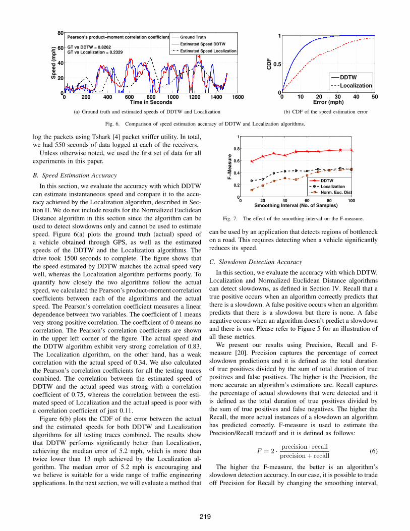
Fig. 6. Comparison of speed estimation accuracy of DDTW and Localization algorithms.

log the packets using Tshark [4] packet sniffer utility. In total,

we had 550 seconds of data logged at each of the receivers.

Unless otherwise noted, we used the first set of data for all

experiments in this paper.

B. Speed Estimation Accuracy

In this section, we evaluate the accuracy with which DDTW

can estimate instantaneous speed and compare it to the accu-

racy achieved by the Localization algorithm, described in Sec-

tion II. We do not include results for the Normalized Euclidean

Distance algorithm in this section since the algorithm can be

used to detect slowdowns only and cannot be used to estimate

speed. Figure 6(a) plots the ground truth (actual) speed of

a vehicle obtained through GPS, as well as the estimated

speeds of the DDTW and the Localization algorithms. The

drive took 1500 seconds to complete. The figure shows that

the speed estimated by DDTW matches the actual speed very

well, whereas the Localization algorithm performs poorly. To

quantify how closely the two algorithms follow the actual

speed, we calculated the Pearson’s product-moment correlation

coefficients between each of the algorithms and the actual

speed. The Pearson’s correlation coefficient measures a linear

dependence between two variables. The coefficient of 1 means

very strong positive correlation. The coefficient of 0 means no

correlation. The Pearson’s correlation coefficients are shown

in the upper left corner of the figure. The actual speed and

the DDTW algorithm exhibit very strong correlation of 0.83.

The Localization algorithm, on the other hand, has a weak

correlation with the actual speed of 0.34. We also calculated

the Pearson’s correlation coefficients for all the testing traces

combined. The correlation between the estimated speed of

DDTW and the actual speed was strong with a correlation

coefficient of 0.75, whereas the correlation between the esti-

mated speed of Localization and the actual speed is poor with

a correlation coefficient of just 0.11.

Figure 6(b) plots the CDF of the error between the actual

and the estimated speeds for both DDTW and Localization

algorithms for all testing traces combined. The results show

that DDTW performs significantly better than Localization,

achieving the median error of 5.2 mph, which is more than

twice lower than 13 mph achieved by the Localization al-

gorithm. The median error of 5.2 mph is encouraging and

we believe is suitable for a wide range of traffic engineering

applications. In the next section, we will evaluate a method that

0 20 40 60 80 1000

0.2

0.4

0.6

0.8

1

Smoothing Interval (No. of Samples)

F−

Me

as

ure

DDTW

Localization

Norm. Euc. Dist

Fig. 7. The effect of the smoothing interval on the F-measure.

can be used by an application that detects regions of bottleneck

on a road. This requires detecting when a vehicle significantly

reduces its speed.

C. Slowdown Detection Accuracy

In this section, we evaluate the accuracy with which DDTW,

Localization and Normalized Euclidean Distance algorithms

can detect slowdowns, as defined in Section IV. Recall that a

true positive occurs when an algorithm correctly predicts that

there is a slowdown. A false positive occurs when an algorithm

predicts that there is a slowdown but there is none. A false

negative occurs when an algorithm doesn’t predict a slowdown

and there is one. Please refer to Figure 5 for an illustration of

all these metrics.

We present our results using Precision, Recall and F-

measure [20]. Precision captures the percentage of correct

slowdown predictions and it is defined as the total duration

of true positives divided by the sum of total duration of true

positives and false positives. The higher is the Precision, the

more accurate an algorithm’s estimations are. Recall captures

the percentage of actual slowdowns that were detected and it

is defined as the total duration of true positives divided by

the sum of true positives and false negatives. The higher the

Recall, the more actual instances of a slowdown an algorithm

has predicted correctly. F-measure is used to estimate the

Precision/Recall tradeoff and it is defined as follows:

F = 2 ·precision · recall

precision + recall(6)

The higher the F-measure, the better is an algorithm’s

slowdown detection accuracy. In our case, it is possible to trade

off Precision for Recall by changing the smoothing interval,

219

as defined in Section III-B. Figure 7 plots the F-measure for

different smoothing intervals for the DDTW, Localization and

Normalized Euclidean Distance algorithms.

The figure illustrates that the F-measure for DDTW is

almost twice as high as the F-measure for Localization and

Normalized Euclidean Distance algorithms across the entire

range of smoothing intervals. This indicates that the DDTW

has higher Precision and Recall compared to the other al-

gorithms. We pick the smoothing interval that achieved the

highest recall value for each algorithm, which in this case,

was 50, 90 and 100 for DDTW, Localization and Norm. Euc.

Dist respectively.

Precision Recall

DDTW 0.68 0.84

Localization 0.38 0.63

Normalized Euclidean Distance 0.39 0.59

TABLE IISLOWDOWN DETECTION PERFORMANCE OF DDTW, LOCALIZATION AND

NORMALIZED EUCLIDEAN DISTANCE ALGORITHMS.

Table II summarizes the Precision and Recall values for

DDTW, Localization and Normalized Euclidean Distance

algorithms for their respective optimal smoothing intervals

derived from their F-Measure in Figure 7. DDTW significantly

outperforms the other two algorithms achieving Precision of

0.68 and Recall of 0.84. Its Precision is 94% higher than

that of Localization and 74% higher than that of Normalized

Euclidean Distance. Its Recall is 40% higher than that of Lo-

calization and 42% higher than that of Normalized Euclidean

Distance.

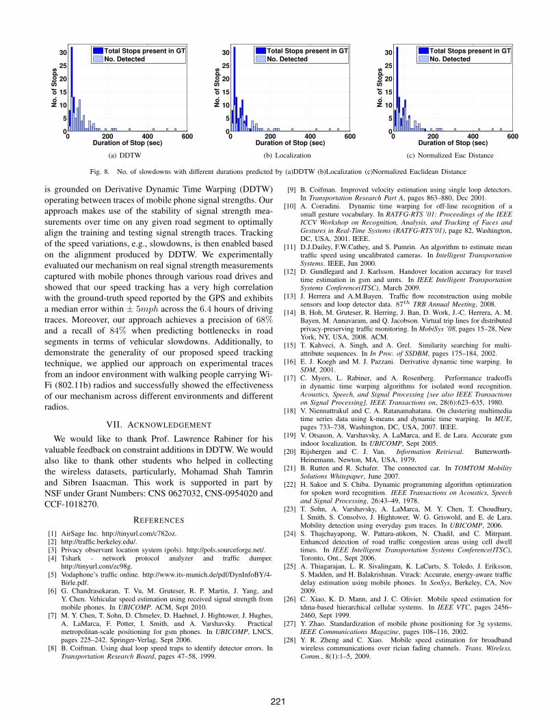
Next, we study the impact of the duration of a slowdown on

the ability of the algorithms to detect it. The intuition tells that

it should be easier to detect slowdowns of a longer duration.

The duration of a slowdown is defined in Section IV as the

total time the speed remains below the threshold of µ mph.

Figure 8 plots a histogram of the number of slowdowns

of a given length that appear in the trace and the number of

slowdowns that are correctly detected by each of the three

algorithms. Although all algorithms can correctly detect all

slowdowns of 120 seconds or more, only DDTW detects all

slowdowns that are longer than 30 seconds. The algorithms

cannot detect slowdowns of a short duration because of the

smoothing that is applied to average out the oscillations in

speed predictions, which in turn results in smoothing out

abrupt speed changes that last for short durations.

D. Effect of Alignment Error on Speed Estimation Accuracy

In this section, we study the effect of the alignment error

between the training and testing traces on the speed estimation

accuracy of DDTW. Recall from Section III that introducing

an alignment error results in applying DDTW on training

and testing traces that are shifted in time by the value of

the alignment error. Note that although we study the effect

of alignment error of up to 500m, a typical GSM based

localization system has a median localization error of less

than 100m [7]. Therefore, it is reasonable to assume that, in

practice, DDTW would achieve speed estimation accuracy that

is equivalent to the one obtained with a 100m alignment error.

Alignment Error(m) Median Error (mph)

0 5.2

100 6.5

200 7.12

500 8.57

TABLE IIIEFFECT OF ALIGNMENT ERROR ON SPEED ESTIMATION ACCURACY

Table III summarizes the median error in miles per hour

for different alignment errors. When a localization systems

provides an accurate location estimate, DDTW suffers from

no alignment errors and has a median speed estimation error

of 5.2 mph. When an alignment error of 100m is present,

the accuracy of DDTW degrades slightly to 6.5 mph. Even in

this case, DDTW performs much better than the Localization

algorithm that achieves the median speed estimation accuracy

of 13 mph.

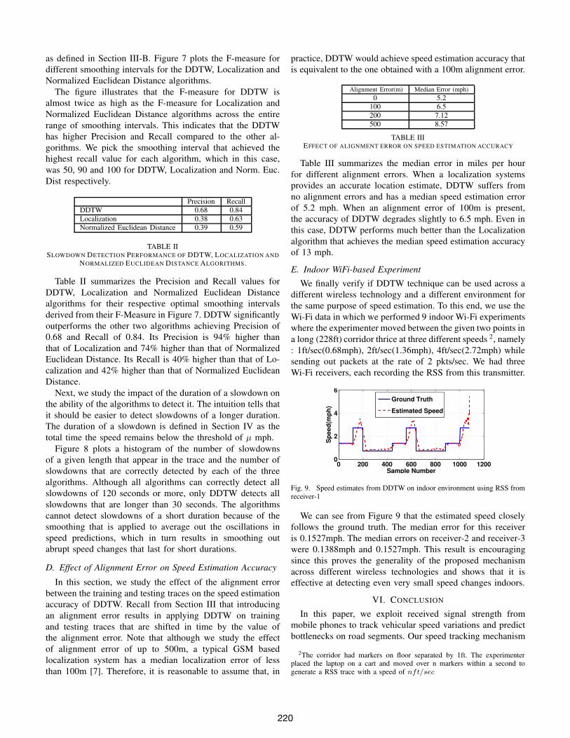
E. Indoor WiFi-based Experiment

We finally verify if DDTW technique can be used across a

different wireless technology and a different environment for

the same purpose of speed estimation. To this end, we use the

Wi-Fi data in which we performed 9 indoor Wi-Fi experiments

where the experimenter moved between the given two points in

a long (228ft) corridor thrice at three different speeds 2, namely

: 1ft/sec(0.68mph), 2ft/sec(1.36mph), 4ft/sec(2.72mph) while

sending out packets at the rate of 2 pkts/sec. We had three

Wi-Fi receivers, each recording the RSS from this transmitter.

0 200 400 600 800 1000 12000

2

4

6

Sample Number

Sp

ee

d(m

ph

)

Ground Truth

Estimated Speed

Fig. 9. Speed estimates from DDTW on indoor environment using RSS fromreceiver-1

We can see from Figure 9 that the estimated speed closely

follows the ground truth. The median error for this receiver

is 0.1527mph. The median errors on receiver-2 and receiver-3

were 0.1388mph and 0.1527mph. This result is encouraging

since this proves the generality of the proposed mechanism

across different wireless technologies and shows that it is

effective at detecting even very small speed changes indoors.

VI. CONCLUSION

In this paper, we exploit received signal strength from

mobile phones to track vehicular speed variations and predict

bottlenecks on road segments. Our speed tracking mechanism

2The corridor had markers on floor separated by 1ft. The experimenterplaced the laptop on a cart and moved over n markers within a second togenerate a RSS trace with a speed of nft/sec

220

0 200 400 6000

5

10

15

20

25

30

Duration of Stop (sec)

No

. o

f S

top

s

Total Stops present in GT

No. Detected

(a) DDTW

0 200 400 6000

5

10

15

20

25

30

Duration of Stop (sec)

No

. o

f S

top

s

Total Stops present in GT

No. Detected

(b) Localization

0 200 400 6000

5

10

15

20

25

30

Duration of Stop (sec)

No

. o

f S

top

s

Total Stops present in GT

No. Detected

(c) Normalized Euc Distance

Fig. 8. No. of slowdowns with different durations predicted by (a)DDTW (b)Localization (c)Normalized Euclidean Distance

is grounded on Derivative Dynamic Time Warping (DDTW)

operating between traces of mobile phone signal strengths. Our

approach makes use of the stability of signal strength mea-

surements over time on any given road segment to optimally

align the training and testing signal strength traces. Tracking

of the speed variations, e.g., slowdowns, is then enabled based

on the alignment produced by DDTW. We experimentally

evaluated our mechanism on real signal strength measurements

captured with mobile phones through various road drives and

showed that our speed tracking has a very high correlation

with the ground-truth speed reported by the GPS and exhibits

a median error within ± 5mph across the 6.4 hours of driving

traces. Moreover, our approach achieves a precision of 68%and a recall of 84% when predicting bottlenecks in road

segments in terms of vehicular slowdowns. Additionally, to

demonstrate the generality of our proposed speed tracking

technique, we applied our approach on experimental traces

from an indoor environment with walking people carrying Wi-

Fi (802.11b) radios and successfully showed the effectiveness

of our mechanism across different environments and different

radios.

VII. ACKNOWLEDGEMENT

We would like to thank Prof. Lawrence Rabiner for his

valuable feedback on constraint additions in DDTW. We would

also like to thank other students who helped in collecting

the wireless datasets, particularly, Mohamad Shah Tamrin

and Sibren Isaacman. This work is supported in part by

NSF under Grant Numbers: CNS 0627032, CNS-0954020 and

CCF-1018270.

REFERENCES

[1] AirSage Inc. http://tinyurl.com/c782oz.[2] http://traffic.berkeley.edu/.[3] Privacy observant location system (pols). http://pols.sourceforge.net/.

[4] Tshark - network protocol analyzer and traffic dumper.http://tinyurl.com/zc98g.

[5] Vodaphone’s traffic online. http://www.its-munich.de/pdf/DynInfoBY/4-Birle.pdf.

[6] G. Chandrasekaran, T. Vu, M. Gruteser, R. P. Martin, J. Yang, andY. Chen. Vehicular speed estimation using received signal strength frommobile phones. In UBICOMP. ACM, Sept 2010.

[7] M. Y. Chen, T. Sohn, D. Chmelev, D. Haehnel, J. Hightower, J. Hughes,A. LaMarca, F. Potter, I. Smith, and A. Varshavsky. Practicalmetropolitan-scale positioning for gsm phones. In UBICOMP, LNCS,pages 225–242. Springer-Verlag, Sept 2006.

[8] B. Coifman. Using dual loop speed traps to identify detector errors. InTransportation Research Board, pages 47–58, 1999.

[9] B. Coifman. Improved velocity estimation using single loop detectors.In Transportation Research Part A, pages 863–880, Dec 2001.

[10] A. Corradini. Dynamic time warping for off-line recognition of asmall gesture vocabulary. In RATFG-RTS ’01: Proceedings of the IEEE

ICCV Workshop on Recognition, Analysis, and Tracking of Faces and

Gestures in Real-Time Systems (RATFG-RTS’01), page 82, Washington,DC, USA, 2001. IEEE.

[11] D.J.Dailey, F.W.Cathey, and S. Pumrin. An algorithm to estimate meantraffic speed using uncalibrated cameras. In Intelligent Transportation

Systems. IEEE, Jun 2000.[12] D. Gundlegard and J. Karlsson. Handover location accuracy for travel

time estimation in gsm and umts. In IEEE Intelligent Transportation

Systems Conference(ITSC), March 2009.

[13] J. Herrera and A.M.Bayen. Traffic flow reconstruction using mobilesensors and loop detector data. 87th TRB Annual Meeting, 2008.

[14] B. Hoh, M. Gruteser, R. Herring, J. Ban, D. Work, J.-C. Herrera, A. M.Bayen, M. Annavaram, and Q. Jacobson. Virtual trip lines for distributedprivacy-preserving traffic monitoring. InMobiSys ’08, pages 15–28, NewYork, NY, USA, 2008. ACM.

[15] T. Kahveci, A. Singh, and A. Grel. Similarity searching for multi-attribute sequences. In In Proc. of SSDBM, pages 175–184, 2002.

[16] E. J. Koegh and M. J. Pazzani. Derivative dynamic time warping. InSDM, 2001.

[17] C. Myers, L. Rabiner, and A. Rosenberg. Performance tradeoffsin dynamic time warping algorithms for isolated word recognition.Acoustics, Speech, and Signal Processing [see also IEEE Transactions

on Signal Processing], IEEE Transactions on, 28(6):623–635, 1980.

[18] V. Niennattrakul and C. A. Ratanamahatana. On clustering multimediatime series data using k-means and dynamic time warping. In MUE,pages 733–738, Washington, DC, USA, 2007. IEEE.

[19] V. Otsason, A. Varshavsky, A. LaMarca, and E. de Lara. Accurate gsmindoor localization. In UBICOMP, Sept 2005.

[20] Rijsbergen and C. J. Van. Information Retrieval. Butterworth-Heinemann, Newton, MA, USA, 1979.

[21] B. Rutten and R. Schafer. The connected car. In TOMTOM Mobility

Solutions Whitepaper, June 2007.[22] H. Sakoe and S. Chiba. Dynamic programming algorithm optimization

for spoken word recognition. IEEE Transactions on Acoustics, Speech

and Signal Processing, 26:43–49, 1978.[23] T. Sohn, A. Varshavsky, A. LaMarca, M. Y. Chen, T. Choudhury,

I. Smith, S. Consolvo, J. Hightower, W. G. Griswold, and E. de Lara.Mobility detection using everyday gsm traces. In UBICOMP, 2006.

[24] S. Thajchayapong, W. Pattara-atikom, N. Chadil, and C. Mitrpant.Enhanced detection of road traffic congestion areas using cell dwelltimes. In IEEE Intelligent Transportation Systems Conference(ITSC),Toronto, Ont., Sept 2006.

[25] A. Thiagarajan, L. R. Sivalingam, K. LaCurts, S. Toledo, J. Eriksson,S. Madden, and H. Balakrishnan. Vtrack: Accurate, energy-aware trafficdelay estimation using mobile phones. In SenSys, Berkeley, CA, Nov2009.

[26] C. Xiao, K. D. Mann, and J. C. Olivier. Mobile speed estimation fortdma-based hierarchical cellular systems. In IEEE VTC, pages 2456–2460, Sept 1999.

[27] Y. Zhao. Standardization of mobile phone positioning for 3g systems.IEEE Communications Magazine, pages 108–116, 2002.

[28] Y. R. Zheng and C. Xiao. Mobile speed estimation for broadbandwireless communications over rician fading channels. Trans. Wireless.

Comm., 8(1):1–5, 2009.

221