Using Mascot to characterise protein modifications - Matrix Science

Tracking fishermen: using GIS to characterise spatial distribution of
fishing effort in the Tasmanian abalone fishery
by Katherine Lesley Tattersall BSc
Submitted in fulfilment of the requirements for
the Degree of Master of Science
University of Tasmania
November 2011
Declaration
This thesis contains no material which has been accepted for a degree or diploma
by the University or any other institution, except by way of background information
and where duly acknowledged in the thesis, and to the best of my knowledge and
belief contains no material previously published or written by another person except
where due acknowledgement is made in the text of the thesis, nor does this thesis
contain any material that infringes copyright.
Signed
Katherine L Tattersall BSc 1st November 2011
i

Statement of Authority
This thesis may be made available for loan and limited copying in accordance with
the Copyright Act 1968.
Katherine L Tattersall 1st November 2011
Statement of Ethical Conduct
The research associated with this thesis abides by the international and Australian
codes on human and animal experimentation, the guidelines by the Australian
Government’s Office of the Gene Technology Regulator and the rulings of the
Safety, Ethics and Institutional Biosafety Committees of the University.
Katherine L Tattersall 1st November 2011
ii

Abstract Major collapses of abalone fisheries around the world have been preceded by a spatial
serial depletion of abalone populations. As in other fisheries, this serial depletion has been
difficult to anticipate and to understand without fine scale monitoring and analysis of spatial
effort distribution. In recent years a field of fisheries science has started to evolve which
looks at the spatial distribution of fishing effort in commercial fisheries and spatial fleet
dynamics, and novel applications of some GIS tools are being developed. Despite the
relative health of the Tasmanian abalone fishery (a $A100 million fishery) compared to other
abalone fisheries around the world, many aspects of the reporting and assessment process
require improvement to ensure sustainability of the fishery. History has shown that reliance
on catch and temporal effort data reported at large spatial scales (current Tasmanian
practice) is inadequate for assessment of abalone stocks, or for detecting spatial depletion.
Traditional fishery independent methods used to estimate population abundance (both
relative and absolute) are also inadequate, and prohibitively expensive for monitoring
fishery stability.
In this study, GPS data loggers were deployed on abalone fishing boats and set to record
latitude and longitude of boat position every ten seconds. Divers wore depth loggers to
record information about when divers were actively fishing. A novel aspect of this study is
the combination of GPS fishing data and GIS tools, generally applied in animal behaviour
analyses, to quantify the spatial distribution of fishing effort as captured by the loggers. The
ability of these methods to describe complexity of diver behaviour, concentration of diver
effort and contraction of the fishery were assessed.
The use of GPS loggers provided high spatial resolution data on fishing activity, and
improved the quality of fishing effort data available. Describing spatial distribution of fishing
effort at fine scales captures information about changes in that spatial distribution.
Performance measures of Catch Per Unit of Area fished were developed and demonstrated
in the context of fishery assessment. Kernel density estimates of fishing activity during
single fishing events are proposed as measures of fishing behaviour. Adoption of simple
behavioural indices (dive duration as an indicator of fishing success) was proposed to
enhance traditional Catch Per Unit Effort based stock-assessment methods. Subject to field
validation, the performance measures developed in this study can be used to forewarn
fishers and advise managers of depleting fish stocks.
iii

Acknowledgements This thesis has been a voyage taken in excellent company. I would like to thank my
supervisors, Craig Mundy, Arko Lucieer and Malcolm Haddon. You each played different
and important roles in the development and completion of this thesis. This project was
conceived by Craig while working as the head of the TAFI Abalone Research Group. Thank
you for your inspiration, your ongoing input, advice and guidance and for giving me the
opportunity to work on such an exciting project. Thank you, Malcolm, for sharing your
expertise, insight and your wide understanding of fisheries management. Arko, you have
helped to guide me from the start and have steered me out of eddies all along the way.
Martin Marzloff provided invaluable advice about the statistics I used in Chapter 3. I often
discussed the ideas behind my work with Martin and he helped me to articulate my thoughts
more clearly.
Thank you to everyone in the Abalone Research Group at TAFI, and in particular to David
Tarbath who helped me to unearth old stock status and assessment reports from pre-MRL
days. To the divers who participated in data collection, a thousand thanks. I hope that you
know how much your contribution has meant to me. I extend my recognition to the
Tasmanian Abalone Council who with the University of Tasmania provided me with a
scholarship to embark on this thesis.
The School of Geography and Environmental Studies at UTAS have provided precious
support and have given me a place to sit, space to think and patience to let me finish this
journey. Rob Anders has come through with ArcGIS support countless times. I would
especially like to thank Jon Osborn for his occasional mentorship and for having faith that I
would reach my destination.
Thank you to Julie Coad, Tracy Payne, Trish McKay and Paulene Harrowby who have
made the administrative side of candidature simple and painless. Thank you to all of the
people at CenSIS for your comradeship and fantastic humour: Phillippa, Michael, Theresa,
Richard, Jenny, Chris and Thor.
My family and my friends have fed me good food, bolstered my morale with bushwalking
plans and kept up a steady stream of cups of tea. Thank you!
iv

TABLE OF CONTENTS
v
TABLE OF CONTENTS Tracking fishermen: using GIS to characterise spatial distribution of fishing effort in
the Tasmanian abalone fishery................................................................................. 1
Declaration.............................................................................................................................. i
Statement of Authority ......................................................................................................... ii
Statement of Ethical Conduct.............................................................................................. ii
Abstract................................................................................................................................. iii
Acknowledgements ............................................................................................................. iv
TABLE OF CONTENTS............................................................................................ 5
LIST OF FIGURES ................................................................................................... 9
LIST OF TABLES ................................................................................................... 15
CHAPTER 1 INTRODUCTION ................................................................................ 1
1.1 A Problem: Abalone fisheries are collapsing ....................................................... 1
1.2 A Culprit: Catch rates as an index of stock abundance ........................................... 2 1.2.1 Abalone fisheries contravene CPUE assumptions ................................................... 3 1.2.2 Mismatch of scale masks stock depletion................................................................. 4 1.2.3 Measures of fishing activity do not capture spatial information ................................ 5
1.3 A Solution: Record the location and spatial extent of fishing activity.................... 6
1.4 Scales of Investigation .................................................................................................. 7
1.5 Aim and Objectives........................................................................................................ 8
CHAPTER 2 DATA COLLECTION AND PROCESSING........................................ 10
2.1 Introduction .................................................................................................................. 10 2.1.1 Objectives ............................................................................................................... 11
2.2 GPS Receiver and Data logger ................................................................................... 11

TABLE OF CONTENTS
vi
2.2.1 Design and Specifications....................................................................................... 11 2.2.2 Sampling Frequency ............................................................................................... 12 2.2.3 Testing for error in GPS data.................................................................................. 14 2.2.4 Identifying fishing events in the GPS data stream.................................................. 15
2.3 Depth/Temperature Logger......................................................................................... 16 2.3.1 Design and Specifications....................................................................................... 17 2.3.2 Clock Drift in Depth Loggers ................................................................................... 18
2.4 Data Collection.............................................................................................................. 20 2.4.1 Raw Data from Loggers .......................................................................................... 20 2.4.2 Matching GPS and Depth Data Streams ................................................................ 21 2.4.3 Compiling a Dataset for Spatial Analysis................................................................ 21
2.5 Discussion of Data Collection Methods .................................................................... 23 2.5.1 Hardware problems.................................................................................................. 24 2.5.2 Hardware deployment and user-related problems .................................................. 24 2.5.3 The cost of multiple data formats............................................................................. 26
CHAPTER 3 SPATIAL DATA AND FISHING EFFORT ANALYSIS ....................... 27
3.1 Introduction .................................................................................................................. 27 3.1.1 Catch Rates as a Measure of Fishery Performance............................................... 27 3.1.2 Abalone abundance vs. abalone availability........................................................... 28 3.1.3 CPUE as an index of availability ............................................................................. 28 3.1.4 Objectives ............................................................................................................... 30
3.2 Methods ........................................................................................................................ 31 3.2.1 Measuring Time: Do accurate measures of dive duration improve CPUE
estimates?......................................................................................................................... 32 3.2.2 Selecting Days for Spatial Catch Rate Analyses.................................................... 33 3.2.3 Measuring Distance: Creating a path of vessel movement ................................... 36 3.2.4 Measuring Area: An index of diver ‘search’ area.................................................... 37 3.2.5 CPUE and CPUA at a fine spatial scale ................................................................. 43 3.2.6. Testing the differences between the different indices: across all divers and for each
diver .................................................................................................................................. 46
3.3 Results .......................................................................................................................... 47 3.3.1 Measuring time: disparities between logger recorded and diver reported dive
times? …………………………………………………………………………………………...47 3.3.2 Selecting Days for Spatial Catch Rate Analyses.................................................... 49 3.3.3 Measuring Distance: Creating a path of vessel movement .................................... 54

TABLE OF CONTENTS
vii
3.3.4 Measuring Area: An index of diver ‘search’ area ................................................... 56
3.4 Case Study: using spatial indices to standardise catch rates................................. 61 3.4.1 Exploring the benefits of spatial effort data.............................................................. 62 3.4.2 Conclusions ............................................................................................................. 65
3.5 Discussion.................................................................................................................... 66 3.5.1 Efficacy of electronic methods for effort capture .................................................... 66 3.5.2 Measuring distance from a path of vessel movement ............................................ 68 3.5.3 Use of GIS tools to calculate spatial structure parameters for fishing events in dive
based fisheries.................................................................................................................. 69 3.5.4 Amalgamation and spatial aggregation of data ...................................................... 72 3.5.5 Indices reflect differences in diver behaviour........................................................... 73
CHAPTER 4 MEASURES OF FISHING BEHAVIOUR: APPLICATIONS OF
ANIMAL BEHAVIOUR SCIENCE ........................................................................... 75
4.1 Introduction .................................................................................................................. 75 4.1.1 What is ‘fishing behaviour’? .................................................................................... 75 4.1.2 (A) Searching behaviour: quantifying complexity of behaviour during a fishing event
.......................................................................................................................................... 77 4.1.3 (B) Behavioural indicators: quantitative summaries of behaviour for whole fishing
events................................................................................................................................ 78 4.1.4 (C) Fleet behaviour: the phenomena of Ideal Free Distribution............................... 78 4.1.5 Objectives ............................................................................................................... 79
4.2 Methods ........................................................................................................................ 80 4.2.1 Spatial complexity of fishing behaviour: Area-based Measures .............................. 80 4.2.2 Spatial complexity of fishing behaviour: Line-based Measures............................... 82 4.2.3 Behavioural indicators: quantitative summaries of behaviour for whole fishing
events................................................................................................................................ 86
4.3 Results .......................................................................................................................... 87 4.3.1 Spatial complexity of fishing behaviour: spatial homogeneity of effort .................... 87 4.3.2 Spatial complexity of fishing behaviour: Line-based Measures.............................. 93 4.3.3 Behavioural indices: quantitative summaries of behaviour for whole fishing events96
4.4 Discussion..................................................................................................................... 99 4.4.1 Spatial complexity of effort distribution .................................................................... 99 4.4.2 Spatial complexity of fishing behaviour: Line-based Measures............................. 102 4.4.3 Behavioural indices................................................................................................ 103 4.4.4 Future directions for research................................................................................ 107

TABLE OF CONTENTS
viii
CHAPTER 5 CONCLUSIONS ............................................................................. 109
5.1 Conclusions of the study........................................................................................... 109 5.1.1 Tools for fishery assessment ................................................................................. 109 5.1.2 Lessons learnt........................................................................................................ 111
5.2 Future directions for research................................................................................... 112
APPENDIX 1: Geoprocessing Inputs and Settings............................................... 114
APPENDIX 2: Frequency distribution of fishing event duration for each diver and for
the East and West coasts ..................................................................................... 116 (i) Aggregation by diver (A, B, C) .................................................................................... 116 (ii) Aggregation by location (east/west coast of Tasmania) ............................................ 118
APPENDIX 3: Changes in Kernel Density Index with increasing fishing event
duration – data table and plots ............................................................................. 119
APPENDIX 4: ANOVA output tables .................................................................... 123
REFERENCES ..................................................................................................... 127
TABLE OF CONTENTS
ix
LIST OF FIGURES Figure 1. Global abalone catch (Haliotis spp.) from 1950 to 2005, from the FAO (FAO 2008).
Tasmanian abalone catch 1965-1974 from the South Eastern Fisheries Committee Abalone fishery
situation report 10 (Dix et al. 1982) and 1974-2005 from the TAFI abalone catch database (TAFI
2008)......................................................................................................................................................1
Figure 2. The Tasmanian abalone fishery is currently managed at the aggregation level of blocks. 57
management blocks were divided into 151 sub-blocks in 2000. ............................................................3
Figure 3. Scales of data aggregation and types of analysis quantifying the complexity and
concentration of diver search patterns for a single fishing event, and distribution and contraction of
effort across the fishery..........................................................................................................................8
Figure 4. A MKI GPS data logger with Haicom Hi-204S GPS receiver and external 12v power supply,
here installed on a diver’s vessel next to the air compressor. Credit: TAFI Abalone Group Image
Collection, 2007. ..................................................................................................................................12
Figure 5. A vessel path was reconstructed from spatial coordinates recorded at regular intervals.
GPS data recorded at (a) 5 second intervals was subsampled at (b) 10 second, (c) 20 second and (d)
1 minute intervals. ................................................................................................................................14
Figure 6. Scatter of recorded GPS locations (projected in WGS84) from two stationary SciElex GPS
data loggers continuously recording position at 10 second intervals for 4 hours in May 2007. ............15
Figure 7. A SensusPro depth and temperature logger, here attached to a diver’s equipment. The
loggers turned on and off automatically when the diver entered and left the water. Credit: TAFI
Abalone Group Image Collection, 2007. ..............................................................................................18
Figure 8. GPS logger and corrected depth logger data plotted for a day of fishing. Four separate
fishing events were recorded by the depth logger on this day, at dive sites in close proximity to each
other. Periods of time when the diver was in the water are highlighted in blue. Between the first and
second dive the vessel briefly reached a speed of almost 17 knots.....................................................19
Figure 9. The contribution of three selected divers to the total number of GPS (with corresponding
depth) records over the first year of the project....................................................................................22
Figure 10. An example of how changes in fishing behaviour may remain undetected using current
CPUE measures, reconstructed from fisher anecdotes. A diver visiting the same location in two
successive years (A and B) found that in the second year they had to search almost three times the
area of the first year to take the same amount of catch. Because they were swimming faster, catch in
Kg/Hr was the same.............................................................................................................................30

TABLE OF CONTENTS
x
Figure 11. Volume and overlap of GPS and depth logger datasets amalgamated to compile a spatial
fishing dataset. (a) Ideally, all depth logger data would be contained within the GPS position dataset
and the fishing duration as measured by the depth logger would approximate fishing duration as
estimated by the diver. (b) In reality, some depth logger data have no corresponding GPS data which
reduced the volume of available spatial fishing data. Also, when fishing duration as estimated by a
diver was significantly greater than the measured depth logger duration, it was possible that some
diving activity was not recorded on the depth logger. ..........................................................................34
Figure 12. A two step algorithm for selecting data from GPS and depth loggers that were appropriate
for calculating daily CPUE estimates. Hoursdl = the sum of dive duration recorded on a depth logger
for all fishing events by one diver on a day, HoursGPS = the total amount of time for which GPS data
were recorded during depth logger recorded dives, by the diver on that day. Hoursdiver was the diver
estimate of time spent fishing on that day (reported to DPIW along with catch in kg). In Step 1, days
were excluded where Hoursdl was greater than HoursGPS with a percentage margin of positive error (x)
permissible. In Step 2, days were excluded when Hoursdiver was greater than Hoursdl, also with a
percentage margin of positive error (y). ...............................................................................................35
Figure 13. Vessel location points (a), sampled at 10 second intervals, are connected with straight line
segments to create a vessel path (b). ..................................................................................................36
Figure 14. Vessel location points (a) for a single fishing event are contained within a Minimum
Convex Polygon (b). The area of the polygon approximates the area searched by the diver. ............39
Figure 15. Divers are tethered to a vessel by the surface supply compressed air hose (yellow in these
photographs). This diver is towing an orange surface buoy on a white line so that his deckhand can
find him easily. Credit: TAFI Abalone Group Image Collection, 2005. ................................................39
Figure 16. Maximum search area available is estimated from a vessel path (a) by buffering to create a
polygon containing all area within 30 m around the path (b). ...............................................................40
Figure 17. While working at a depth of approximately 20 m, a 30 m hose will not allow a diver to be
much more than 20m from the vessel. .................................................................................................41
Figure 18. 95% of vessel location points (a) for a single fishing event are contained within the 95%
contour of a KDE raster surface (b). ....................................................................................................42
Figure 19. Extracts from a map showing every fishing event to which catch rates were allocated.
CPUE (kg/hr) (a), CPUD (kg/km) (b) and CPUA (kg/ha) (c) estimates were calculated daily and
allocated to all fishing events that contributed to the day’s catch. A 500m grid was imposed on the
map. CPUE estimates were aggregated and the mean calculated across grid cells (d). Values were
colour coded: Dark green: 0-40 kg/hr, Mid-green:40-80 kg/hr, Light green: 80-120 kg/hr....................46
Figure 20. Relationship between fishing time estimated by divers (Hoursdiver) and fishing time
recorded by the depth loggers (Hoursdl). If depth logger values were correct, diver estimates would be

TABLE OF CONTENTS
xi
both inaccurate and imprecise. An perfect diver estimate would fall on the red line (i.e. Hoursdiver =
Hoursdl). ...............................................................................................................................................48
Figure 21. Frequency distribution of the discrepancy (minutes) between fishing time recorded by depth
loggers (Hoursdl) and fishing time estimated by divers (Hoursdiver).......................................................49
Figure 22. Step 1 of the exclusion algorithm: Modelling the effects of different values of accepted
disparity (as a proportion of Hoursdl) on data retention. The vertical dotted line illustrates the outcome
when the disparity is equal to or less than 10% of Hoursdl. ..................................................................50
Figure 23. Step 2 of the exclusion algorithm: the percentage of days of data retained for CPUE
analysis as a function of discrepencies in dive duration.......................................................................51
Figure 24. Days of data kept following the data exclusion algorithm (shown in orange) for Diver A.
Points falling above the blue line were excluded at a +30% exclusion rate in step 2 (cf Figure 23). An
accurate diver estimate (Hoursdiver equal Hoursdl) falls on the red line when the depth logger captured
all dive data (i.e. was deployed on all dives for a day). ........................................................................52
Figure 25. Frequency distribution of catch per unit of distance CPUD (kg/km) for each of three divers
A, B and C............................................................................................................................................55
Figure 26. Distribution plots of estimated potential daily diver search area, for all divers, calculated
with three techniques: MCP (Amcp), buffer (Abuf) and KDE 95% contour (Akde). The three area
estimates are significantly different from each other (Student’s t-test P = 0.05). Green diamonds mark
Mean and Standard Error for each distribution. ...................................................................................56
Figure 27. A multivariate scatterplot matrix of daily estimates of Amcp, Abuf and Akde. N = 147. Note
different scales on axes. In pairwise correlations, the strongest correlation between area estimates
was between Abuf and Amcp with a correlation of 0.85 and Akde and Abuf with a correlation also of 0.85.
Correlation between Amcp and Akde was 0.66........................................................................................57
Figure 28. Frequency distribution of Akde (ha) for each day, for each of Divers A (a), B (b), and C (c).
Note the different scales on the y-axes. Quantile box plots for each distribution are given. Cf Table 7.
.............................................................................................................................................................58
Figure 29. Catch per unit of area (kg.ha-1) derived from Amcp (a), Abuf (b) and Akde (c) plotted against
CPUE (kg.hr-1) for each of three divers A (solid blue dots), B (solid red dots) and C (black diamonds).
Similar x and y scales are used to facilitate visual comparison............................................................60
Figure 30. The site described in this case study is the most intensively fished in the Tasmanian
abalone fishery. This figure represents 13 days of fishing by one diver. Red dots represent the
centroid of each fishing event. KDE analyses were performed for each fishing event and 50% (light
blue) and 90% (dark blue) contours of potential effort distribution are displayed in this figure.............62
TABLE OF CONTENTS
xii
Figure 31. Association between CPUE (diver estimated time) and measures of Catch Per spatial Unit
of effort using data recorded by the logger (hr, ha, km). a) CPUEdiver against CPUEdl. b) Measures of
effort that include spatial distribution based upon units of area (CPUA) or of distance (CPUD). Each
measure of effort that includes spatial distribution gives a different pattern of catch rate relative to the
traditional CPUE. .................................................................................................................................63
Figure 32. Eight data points derived from the 13 days of fishing activity illustrated in the map in Figure
30. There is a negative correlation between search rate and catch rate up to a threshold catch rate
(Kg/Hr). Above the threshold, search rate is almost constant despite increasing catch rates. .............65
Figure 33. The concentration of vessel location points for a single fishing event can be described by
finding the ratio of the area contained within the 50% contour of a KDE raster surface (a) to the area
contained within the 95% contour (b). Cf. Figure 18. ...........................................................................81
Figure 34. The log normal frequency distribution of values of KDI, with an outlier box plot. The ends
of the box are the 25th and 75th quantiles, the line in the middle of the box identifies the median
sample value and the means diamond indicates the sample mean and 95% confidence interval.
Possible outliers are outside of: upper quartile + 1.5*(interquartile range) and lower quartile -
1.5*(interquartile range). ......................................................................................................................88
Figure 35. Contour maps of fishing events with kernel density ratios ranging from very low (a) to very
high (i). Proportion of total dive time is shown as a percentage in the colour legend. Note different
scales of distance. See values of calculated ratios in Table 9. ...........................................................89
Figure 36. Bivariate plots of KDI expressed as a percentage against area of the 95% contour polygon
(a) and fishing duration (b). ..................................................................................................................90
Figure 37. KDE 50 and 95 percent contours for a single dive, representing changes in KDI from 10
minutes after start (a) until the end of the dive (i) at 142 minutes. Contours overlay a 5 metre scale
grid. See Appendix 3 for data tables and all contours in 10 minute increments. The KDI values for
these increments are plotted in Figure 38. ...........................................................................................92
Figure 38. KDI values as percentages, simulated from a single fishing event by dividing the event into
10-minute segments. KDE 50 and 95 percent contours were generated for each cumulative 10-
minute fraction of the dive (C.f. Figure 37). These are data at a scale finer than even single fishing
events, and can be used to differentiate between periods of rapid movement and slow movement
during a fishing event. ..........................................................................................................................93
Figure 39. Mean vessel velocity for each fishing event in this study (n=979), plotted against WGS84
UTM 55S Eastings. The boundary between ‘east’ and ‘west’ coast fisheries is at 490,000 m. A
horizontal red line demarcates the mean value 28.12 (SD = 44.61). A frequency distribution plot on the
right y-axis shows velocity outliers above 50m/min..............................................................................94
Figure 40. Median vessel velocity for each fishing event grouped by Diver (a) and by coast (b). A non-
parametric Kruskal-Wallis test found that there are significant differences in median vessel velocity

TABLE OF CONTENTS
xiii
between all divers (A: n=228, B: n=436, C: n=320) and between aggregated east and aggregated
west coast data (E: n=439, W: n=540). ................................................................................................94
Figure 41. The frequency distribution of path sinuosity values calculated using Hawth’s Analysis Tools.
Paths for which sinuosity >50 (1.3%) were excluded from the plot to show remaining data more
clearly. The median value is 6.26. The ends of an outlier box plot mark the 25th and 75th quantiles,
the line across the middle of the box identifies the median sample value and the means diamond
indicates the sample mean and 95% confidence intervals. Possible outliers are outside of upper
quartile + 1.5*(interquartile range)........................................................................................................95
Figure 42. Frequency distribution of the duration of fishing events across all divers and the entire
fishery. In the 15-20 minute bin there were 58 events, in the 20-25 minute bin only 29, and in the 25-
30 minute bin 61 fishing events. There is a break in dive duration at 20-25 minutes (red bar in the
histogram). ...........................................................................................................................................96
Figure 43. West Coast: Diver depth for each fishing event plotted against WGS84 UTM zone 55S
centroid easting (on the x-axis). N=550, Maximum mean depth=14.8m, Mean=6.3m. Frequency
distribution of easting is on the top horizontal axis and depth on the right vertical axis. The coloured
lines represent quantile density contours at 5% increments. ...............................................................98
Figure 44. East Coast: Diver depth for each fishing event plotted against WGS84 UTM zone 55S
centroid easting (on the x-axis). N=439, Maximum mean depth=14.8m, Mean=6.2m. Frequency
distribution of easting is on the top horizontal axis and depth on the vertical axis. Density contours are
at 5% increments. ................................................................................................................................98
Figure 45. Frequency distribution of mean dive depth (for a fishing event) on the west (a) and east (b)
coasts. Distribution on the west coast is log-normal (N= 550, Mu=1.72, Sigma=0.50, KSL Goodness
of Fit D=0.040285, P=0.0373) and distribution on the east coast is normal (N=439, mu=6.20,
Sigma=2.46, Shapiro-Wilk Goodness of Fit W=0.990693, P=0.0072). Percentage frequency is
reported at the top of each histogram bin.............................................................................................99
Figure 46. (a) Expected patterns of diver visitation for four hypothetical stock scenarios. (a) Stable,
abundant stock: very few unsuccessful fishing events and many successful events. (b) Stable
unproductive stock: no successful fishing events and very few ‘exploratory’ unsuccessful events. (c)
Stock depletion and subsequent recovery: a pattern of declining numbers of successful fishing events
and increasing numbers of unsuccessful events after stock collapse, and a reverse in trends as stocks
recover. (d) Stock depletion or collapse: declining frequency of diver return to a fishing location
suffering from stock depletion or collapse. At a crucial level of stock depletion, successful fishing
events decline in number as unsuccessful fishing events become more frequent. With time, divers
stop returning to the site.....................................................................................................................105
Figure 47. Diver A: frequency distribution of fishing event duration with an outlier box plot showing the
25th and 75th quantiles (ends of box) median (solid line), sample mean with 95% confidence interval
(diamond) and outliers outside of the upper (lower) quartile +(-) 1.5 times the interquartile range. ...116

TABLE OF CONTENTS
xiv
Figure 48. Diver B: frequency distribution of fishing event duration with an outlier box plot showing the
25th and 75th quantiles (ends of box) median (solid line), sample mean with 95% confidence interval
(diamond) and outliers outside of the upper (lower) quartile +(-) 1.5 times the interquartile range. ...117
Figure 49. Diver C: frequency distribution of fishing event duration with an outlier box plot showing the
25th and 75th quantiles (ends of box) median (solid line), sample mean with 95% confidence interval
(diamond) and outliers outside of the upper (lower) quartile +(-) 1.5 times the interquartile range. ...117
Figure 50. East coast: frequency distribution of fishing event duration with an outlier box plot showing
the 25th and 75th quantiles (ends of box) median (solid line), sample mean with 95% confidence
interval (diamond) and outliers outside of the upper (lower) quartile +(-) 1.5 times the interquartile
range..................................................................................................................................................118
Figure 51. West coast: frequency distribution of fishing event duration with an outlier box plot showing
the 25th and 75th quantiles (ends of box) median (solid line), sample mean with 95% confidence
interval (diamond) and outliers outside of the upper (lower) quartile +(-) 1.5 times the interquartile
range..................................................................................................................................................118
TABLE OF CONTENTS
xv
LIST OF TABLES Table 1. Specifications of ReefNet depth and temperature loggers (ReefNet 2002b).........................17
Table 2. The total number of 10 second fishing records for each of the three divers A, B and C, also,
the number of defined individual fishing ‘events’ for each diver in each month....................................23
Table 3. Summary of the catch rate indices generated in chapter 3. ...................................................44
Table 4. Catch rates calculated for each diver on each day were allocated to individual fishing events.
Catch rates were assigned to 628 individual fishing events between the beginning of July 2005 and
end of April 2007. .................................................................................................................................45
Table 5. Summary of data exclusions for each diver............................................................................51
Table 6. The sum of path lengths (m) for each day. One outlier was excluded from datasets for each
of Diver B and Diver C. ........................................................................................................................54
Table 7. Descriptive statistics for the frequency distributions of Akde (ha) for Divers A, B and C. Cf.
Figure 28..............................................................................................................................................59
Table 8. Fishing activity of one diver working the Acteon Reef between January 2006 and April 2007
.............................................................................................................................................................62
Table 9. Calculated KDI for the fishing events in Figure 35 (a to i): n = the number of location points
recorded. A low KDI (e.g. <0.05) indicates that half of the fishing event was spent in a small part (e.g.
<5%) of the total area covered during the dive, and thus that effort distribution was heterogeneous. .90
Table 10. The changing value of KDI as the duration of a fishing event increases. ..........................119
Table 11. Results of the 2-way ANOVA testing effects of individual divers (Diver) and area-estimating
methods (Method: Abuf, Amcp or Akde) on search area (log-transformed).............................................124

CHAPTER 1 – INTRODUCTION
1
CHAPTER 1 INTRODUCTION
1.1 A Problem: Abalone fisheries are collapsing
Abalone are marine molluscs that are expensive gastronomic delicacies in many
parts of Asia. The growth of international trade in the last century has meant that
intense fishing pressure has been placed on wild populations of abalone. Because
of excessive fishing pressure USA abalone stocks have regressed from valuable
fisheries to being in a state of commercial non-viability (Figure 1). The British
Columbia fishery was closed in 1990 and through the 1990’s there was no evidence
of significant fishery recovery (Jamieson 2001). The Mexican abalone fishery has
also suffered from over-fishing and while still viable it is operating at a much smaller
scale than previously (Leiva and Castilla 2001). The South African abalone fishery
was closed on the 1st of November 2007 (Benton 2007). Due to this string of
fishery collapses and closures elsewhere, Australia now supports the most
productive wild fishery for abalone in the world. Tasmania is currently the source of
almost half of Australia’s abalone catch and in 2005 was the source of 28% of
global catch (calculated from FAO catch records and Tasmanian catch reporting
records from the Tasmanian Aquaculture and Fisheries Institute).
0
2000
4000
6000
8000
10000
12000
14000
16000
18000
1950 1955 1960 1965 1970 1975 1980 1985 1990 1995 2000 2005
Years
Qua
ntity
(t) (
x100
0)
Mexico United States of America Japan
Australia New Zealand Tasmania
2
4
6
10
18
14
16
12
8
0.000.331.041.772.49
5.59
Figure 1. Global abalone catch (Haliotis spp.) from 1950 to 2005, from the FAO (FAO 2008).
Tasmanian abalone catch 1965-1974 from the South Eastern Fisheries Committee Abalone
fishery situation report 10 (Dix et al. 1982) and 1974-2005 from the TAFI abalone catch
database (TAFI 2008).

CHAPTER 1 – INTRODUCTION
2
1.2 A Culprit: Catch rates as an index of stock abundance
Abalone fisheries traditionally have been managed using trends in Catch Per Unit
Effort (CPUE) as indicators of stock abundance. CPUE is defined as the amount of
catch taken by a vessel or by a fleet with application of a defined unit of effort
(Breen 1992). Across a range of fisheries, effort can be measured using several
different dimensions including duration of trawling, gear units (e.g. number of hooks
in a set) (Bordalo-Machado 2006) and for abalone fisheries worldwide the number
of hours spent diving (Breen 1992). In Tasmania, CPUE is reported by abalone
divers to the State fisheries management organisation (Fisheries Branch,
Department of Primary Industries, Parks, Water and Environment) through a paper
docket system. Daily catch is reported in kilograms, and the time spent diving for
each day is estimated and reported in hours (Tarbath et al. 2007). Catch and
associated effort is reported within defined spatial units (blocks). The size of
reporting blocks range from 20km to 60km. Thus, the scale at which fishing activity
is captured spans 10’s of kilometres of coastline. In Tasmania, there are 57
abalone blocks, divided into 151 sub-blocks (Figure 2). In addition, the fishery is
formally divided into separate zones to ensure effort is distributed sustainably. In
2007, the Tasmanian blacklip (Haliotis rubra) fishery was partitioned into Eastern,
Western, Northern and Bass Strait zones, with a further greenlip (Haliotis laevigata)
specific zone (Tarbath et al. 2007).
It is generally accepted that reliance on CPUE as a key performance measure has
contributed to management failure in abalone fisheries worldwide. CPUE was used
for stock assessment for fisheries in California and Mexico prior to their collapse
(Karpov et al. 2000). Despite this, abalone fishery assessments in Tasmania and
world-wide still rely heavily on catch rate recorded at relatively coarse spatial scales
as the principle performance measure (Prince 2005).

CHAPTER 1 – INTRODUCTION
3
Figure 2. The Tasmanian abalone fishery is currently managed at the aggregation level
of blocks. 57 management blocks were divided into 151 sub-blocks in 2000.
1.2.1 Abalone fisheries contravene CPUE assumptions
CPUE is not an ideal stock assessment tool or performance measure for abalone
fisheries because these effort measures contravene key assumptions upon which
the method relies, i.e. that across a sampled area:
• the stock is homogenous in distribution and
• fishing is randomly distributed (Salthaug and Aanes 2003)
All abalone species are patchily distributed and are made up of extensive meta-
populations (Shepherd and Brown 1993, Morgan and Shepherd 2006) within which
the many sub-populations can have different biological properties of growth and
productivity (Prince 2003). Under the same fishing conditions, some sub-
populations will persist while others can not sustain themselves (Prince 2005).
Given the typical distribution patterns of most haliotids, the assumption of
homogeneous stocks is rarely valid. The fragmented spatial structure of meta-
populations leads to fragmented fishing behaviour and non-random distribution of
fishing effort (Karpov et al. 2000).
CHAPTER 1 – INTRODUCTION
4
2005).
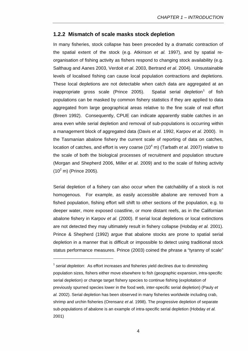
1.2.2 Mismatch of scale masks stock depletion
In many fisheries, stock collapse has been preceded by a dramatic contraction of
the spatial extent of the stock (e.g. Atkinson et al. 1997), and by spatial re-
organisation of fishing activity as fishers respond to changing stock availability (e.g.
Salthaug and Aanes 2003, Verdoit et al. 2003, Bertrand et al. 2004). Unsustainable
levels of localised fishing can cause local population contractions and depletions.
These local depletions are not detectable when catch data are aggregated at an
inappropriate gross scale (Prince 2005). Spatial serial depletion1 of fish
populations can be masked by common fishery statistics if they are applied to data
aggregated from large geographical areas relative to the fine scale of real effort
(Breen 1992). Consequently, CPUE can indicate apparently stable catches in an
area even while serial depletion and removal of sub-populations is occurring within
a management block of aggregated data (Davis et al. 1992, Karpov et al. 2000). In
the Tasmanian abalone fishery the current scale of reporting of data on catches,
location of catches, and effort is very coarse (104 m) (Tarbath et al. 2007) relative to
the scale of both the biological processes of recruitment and population structure
(Morgan and Shepherd 2006, Miller et al. 2009) and to the scale of fishing activity
(102 m) (Prince
Serial depletion of a fishery can also occur when the catchability of a stock is not
homogenous. For example, as easily accessible abalone are removed from a
fished population, fishing effort will shift to other sections of the population, e.g. to
deeper water, more exposed coastline, or more distant reefs, as in the Californian
abalone fishery in Karpov et al. (2000). If serial local depletions or local extinctions
are not detected they may ultimately result in fishery collapse (Hobday et al. 2001).
Prince & Shepherd (1992) argue that abalone stocks are prone to spatial serial
depletion in a manner that is difficult or impossible to detect using traditional stock
status performance measures. Prince (2003) coined the phrase a “tyranny of scale”
1 serial depletion: As effort increases and fisheries yield declines due to diminishing
population sizes, fishers either move elsewhere to fish (geographic expansion, intra-specific
serial depletion) or change target fishery species to continue fishing (exploitation of
previously spurned species lower in the food web, inter-specific serial depletion) (Pauly et
al. 2002). Serial depletion has been observed in many fisheries worldwide including crab,
shrimp and urchin fisheries (Orensanz et al. 1998). The progressive depletion of separate
sub-populations of abalone is an example of intra-specific serial depletion (Hobday et al.
2001)

CHAPTER 1 – INTRODUCTION
5
balone (Beinssen
1979).
to articulate the mismatch in scales of reporting and fishing. Prince also asserts that
research and monitoring of highly structured stocks like abalone is prohibitively
expensive and generally not done well, if at all. Given the poor performance of
CPUE based performance measures, there remains a management need for
alternative fishery performance measures that can capture the fine scale spatial
nature of abalone fisheries and that can act as proxies for stock abundance.
Intra-specific serial depletion of fisheries can occur in two different ways: 1) In the
absence of size limits, it is the sequential removal or extinction of populations (e.g.
fishery declines in California, Mexico and Japan); 2) With size limits (intended to
maintain a sufficient number of mature individuals) but with an unsustainable Total
Allowable Catch, it is the sequential depletion of fishable populations beyond the
productivity of those populations (e.g. West coast of Tasmania) (Mundy 2005). In
the latter case, if allowed sufficient time, there is good biological reason to expect
that these populations will recover. Recovery time will depend on the productivity
of individual populations (Morgan and Shepherd 2006).
1.2.3 Measures of fishing activity do not capture spatial information
In addition to the mismatch of scales of fishing activity and catch reporting, each
fishing event2 encompasses diver behaviour that has a spatial component not
taken into account by current catch rate estimates. Unlike the units used to
measure effort in trawl fisheries (duration of trawling in h hours with n gear units
travelling at x speed) (Bordalo-Machado 2006), abalone fishing effort measured in
hours does not integrate any spatial information (distance, area, volume). It is not
possible to know whether a diver has searched a large or small area to take their
catch when data on the very fine scale distribution of fishing effort during a day is
not available. If the density of abalone varies at different places or times, a diver
may search a greater area to take the same amount of catch, possibly within the
same amount of time. The speed at which a diver swims can also be highly
variable and dependent on the abundance and distribution of a
2 fishing event: a single dive event, commencing when a diver enters the water and ending
when the diver leaves the water.

CHAPTER 1 – INTRODUCTION
6
1.3 A Solution: Record the location and spatial extent of
fishing activity
Detailed information on fishing location would enable calculation of site-specific
CPUEs. Data on diver swim speed and search patterns could provide the spatial
variables (speed, volume/area) that are available when calculating CPUE for a trawl
vessel, but these parameters are not available when calculating catch rate in an
abalone fishery. Babcock et al. (2005) describe a need for the knowledge and skills
of landscape ecologists, who work with spatial data in a GIS environment, to be
integrated with the knowledge and skills of fisheries scientists, who use population
dynamics models and statistical tools for fisheries management. They propose that
cooperation between these fields of research would progress the design of spatial
management measures and help prevent bias in trends caused by spatial
heterogeneity.
Global Positioning System (GPS) loggers have offered a significant advance in
techniques for studies of fine-scale animal movement patterns (Ryan et al. 2004).
In the field of animal behaviour studies, Geographical Information System (GIS)
analysis tools have been developed to investigate the relationship between foraging
patterns of predators and spatial distribution of prey, e.g. Ramos-Fernandez et al.
(2004), Garthe et al. (2007). If measures of fisher behaviour can provide reliable
alternative estimates of CPUE/stock abundance, as demonstrated in a novel
application for the Peruvian trawl fishery (Bertrand et al. 2004, Bertrand et al. 2005)
then these measures may become valuable as abalone fishery performance indices
that can be used independently of CPUE.
Two spatial issues could be addressed with fine-scale spatial information; the
precise location of the site of fishing effort expenditure, and development of a
spatial performance index that captures the response of a diver to stock density. In
the absence of tested alternative measures, a CPUE estimate that integrates fine
scale spatial patterns will be more informative to managers than CPUE calculated
at a scale of management blocks. Fine-scale changes in CPUE could indicate a
change in local availability of abalone. If effort is measured with a spatial or
volumetric component instead of only in hours, fluctuations in abalone density may
be captured. Quantitative metrics that describe fishing behaviour could eventually
link foraging behaviour to prey abundance. New spatial performance measures that

CHAPTER 1 – INTRODUCTION
7
do not assume random fishing will, ideally, eventually supplement or replace
traditional fishery statistics in abalone fishery stock assessment.
Through this study I tested spatial analysis techniques that may be used in
conjunction with each other to improve management decisions in three major ways:
1) by focusing on estimates of CPUE at the scale at which fishing occurs,
i.e. at the scale of an individual diver harvesting sub-populations of
abalone rather than across the whole fleet at the scale of management
blocks.
2) By using fine-scale spatial information about individual fishers’ behaviour
to integrate the spatial component of fishing activity into distance- and
area-based indices of fishing effort;
3) By developing a spatial behaviour-based index of fishing performance
independent of CPUE that can be used in parallel with catch rate
information to quantify the degree of non-randomness and non-
homogeneity of diver fishing behaviour.
In order to develop these techniques, data have been collected with the
cooperation of a subset of divers within the Tasmanian abalone industry. These
volunteer project participants carried GPS data loggers on their vessels and
depth/temperature loggers on their person while diving. The data collected were
both spatial and temporal and included precise location, time and depth of fishing
activity. The data collection methods are described in detail in Chapter 2.
1.4 Scales of Investigation
For this thesis, diver data have been aggregated and analysed at two different
scales: a) diver dynamics during a single fishing event, and b) fleet dynamics
across multiple fishing events (Figure 3).

CHAPTER 1 – INTRODUCTION
8
VESSEL GPS DATA DIVER DEPTH DATA
Spatial and Temporal Dataset
• Area searched in a dive event
• Duration of dive event
• Length of vessel track
Distribution of fishing grounds
Diver dynamics Fleet dynamics
Linear analyses
CONCENTRATION CONTRACTION
• Sinuosity of vessel track
• Fractal dimension of vessel track
COMPLEXITY
• Kernel density estimate
• Concentration index
Area-based analyses
• Extent of fishing grounds
• Total area fished
• Temporal changes in area fished
• Overlap of dive events
• Depth of dive events
CPUE
Inco
rpor
atin
g sp
atia
l m
easu
res
of e
ffort
Figure 3. Scales of data aggregation and types of analysis quantifying the complexity and
concentration of diver search patterns for a single fishing event, and distribution and
contraction of effort across the fishery.
1.5 Aim and Objectives
Using the example of the Tasmanian abalone fishery, the aim of this study is to test
and illustrate the value of collecting fine-scale spatial information about the fishing
activity of individual fishers to support monitoring, assessment and management of
a small-vessel coastal fishery.
In this thesis, four main objectives are addressed:
1. Firstly, in Chapter 2, I present the methods used to collect fine-scale spatial
data from a small sample (three volunteer divers) of the Tasmanian abalone
fishery. Based on the successes and impediments encountered during this
exploratory sampling of fine-scale fishing activity, recommendations are
made to guide future studies;
2. In Chapter 3, I describe a range of indices of fishing effort derived from fine-
scale monitoring of fishing activity. I identify a number of spatial analysis
methods and GIS tools that can be applied to quantify fine scale spatial
abalone catch and effort data and demonstrate the application of these
methods to fisheries data. Due to unanticipated technical failures that
occurred during sampling, data had to be filtered prior to analysis. Only a
subset of data from three individual divers was used to test the value of fine-
CHAPTER 1 – INTRODUCTION
9
scale monitoring of fishing effort to complement traditional measures of
fishing activity (CPUE) with some alternative distance-based and area-
based indices of fishing effort;
3. In Chapter 3, I also assess the ability of these fine-scale indices of fishing
activity to distinguish different fishing behaviours and identify different sub-
groups of behaviour within data sets;
4. In Chapter 4 I focus on area-based measures of divers’ abalone harvesting
behaviour as indices to capture concentration of diver effort. Such spatial
indices can potentially provide catch-independent information about fine-
scale fishing efficiency. I also discuss limitations of the indices.

CHAPTER 2 – DATA COLLECTION AND PROCESSING
CHAPTER 2 DATA COLLECTION AND PROCESSING
2.1 Introduction
Since 2005, researchers at the Tasmanian Aquaculture and Fisheries Institute
(TAFI) have been developing electronic tools to improve the quality and resolution
of fishery dependent data in the Tasmanian abalone fishery, a dive fishery. These
tools are a passive Global Positioning System (GPS) data logger to record fine
scale spatial information on the location of fishing activity, and an automatic
depth/temperature recorder to obtain an accurate record of time and depth of each
fishing event. The research has been funded by TAFI and in 2006, additional
funding was received from the Australian Fisheries Research and Development
Corporation (FRDC) to continue the development process (FRDC 2006/029). Diver
participation in the research program is voluntary and participation numbers have
increased from two divers in 2005, to approximately 20 divers in 2007. This
represents twenty percent of the active divers working in the fishery.
The collection of fine scale fishery dependent data for a dive fishery is a novel
undertaking and the data logging approach has been developed to complement the
particular way that an abalone diver works while fishing. In the Tasmanian fishery,
abalone divers generally work from a ‘live’ (i.e. not anchored and with motor
running) vessel that is driven by a deckhand. The deckhand is also responsible for
the compressor that supplies air to the diver through a high-pressure hose, for
deploying empty catch bags to, and retrieving full bags from the diver, and packing
abalone into bins. Divers travel from boat ramp to dive site either on a small vessel
(~16 ft) or, for more remote locations, on a ‘mother ship’, a larger boat carrying one
or more smaller tenders and with facilities to store live abalone for extended
periods.
On arrival at a dive site, divers enter the water with an abalone iron (a bar used to
lever or flick abalone from reef and rocky substrates) and collect abalone across
the extent of the reef or site. Different divers may have different search and fishing
patterns, and these patterns are highly likely to be influenced by the weather (wind
speed and direction and swell height), visibility conditions, macroalgal density,
depth, bathymetry and surface or reef roughness, and potentially other factors.
While fishing, deckhands will drive the vessel to follow a diver, being directly above
10

CHAPTER 2 – DATA COLLECTION AND PROCESSING
the diver when retrieving catch bags and in reasonably close proximity to the diver
for the full duration of a fishing event. When a diver exits the water, the vessel may
travel over distance to a different dive site to continue fishing. A GPS data logger
captures data on vessel location throughout each dive and an automatic
depth/temperature logger captures the time of diver entry to and exit from the
water, and the depth profile of the dive. These data sets were combined to identify
the location of the vessel when the diver was in the water.
2.1.1 Objectives
The objectives of this chapter are to:
• Describe the equipment used to collect fine scale spatial data from abalone
divers working in the Tasmanian fishery.
• List the parameters that are measured by this equipment.
• Outline the dataset that was compiled for spatial analysis in this thesis.
• Identify problems encountered during data collection for this project.
2.2 GPS Receiver and Data logger
2.2.1 Design and Specifications
GPS Data loggers (MK0) for the project were designed to TAFI specifications by
SciElex, a marine electronics company based in Kingston, Tasmania (Cfish 2004).
Starting in 2004, two progressively more flexible models of GPS data logger were
developed (MKI, MKII). Each of the GPS loggers had integrated non-differential 12
channel GPS receivers. The Haicom Hi-204S was used in all earlier models (MK0
and MKI loggers). The MK0/MKI loggers recorded standard National Marine
Electronics Association (NMEA) output data from the receiver with date and time in
UTC0, and had a capacity of 1,048,576 records (approximately 120 days of
continuous recording at 10 sec intervals, 24 hours/day). The datum for Latitude and
Longitude was WGS84. The manufacturer’s specifications for the Hi-204S listed
accuracy as 25m (Haicom_Electronics_Corporation 2005). Both MK0 and MKI
GPS loggers required an external 12V power supply. On diver’s boats, power was
supplied to these GPS loggers either from on-board power or from a sealed lead-
acid 12V battery (see Figure 4). MKII GPS loggers were powered internally by 4 x
1.2v batteries in series providing 4.8V for approximately 40 hours of run time, and
11

CHAPTER 2 – DATA COLLECTION AND PROCESSING
used a Fastrax uPatch100-S GPS receiver (Fastrax Limited 2006)3. Standard
NMEA strings were captured from the module. Memory in the MKII loggers was a
128MByte Flash Card providing capacity for more than 2 million samples. Each
GPS receiver and logger was encased in a robust, waterproof housing (Figure 4).
Data were downloaded from the MK0 and MKI GPS data loggers via a serial port
using the Windows HyperTerminal interface. Data were saved in standard NMEA
format to a CSV file. The MKII GPS loggers were supplied with download software
which performed some basic data management functions such as conversion of
raw time and date fields into a combined date/time field in a user selected UTC time
zone.
Figure 4. A MKI GPS data logger with Haicom Hi-204S GPS receiver and external 12v
power supply, here installed on a diver’s vessel next to the air compressor. Credit: TAFI
Abalone Group Image Collection, 2007.
2.2.2 Sampling Frequency
Provided that there was adequate satellite reception, the GPS data loggers were
capable of recording a constant stream of position data at any sampling frequency
up from one second intervals. Turchin (1998) stated that when sampling movement
paths the sampling frequency should match the scale of change or the scale of
movement4. As this research project was focussed on capturing and quantifying
3 Two MKII loggers (MKIIA) were produced with Haicom Hi-204S GPS receivers. Data from
these loggers were not used in analyses, for reasons outlined in Ch 2 Section 2.3. 4 Inappropriate sampling frequency is referred to as undersampling, or oversampling.
Undersampling can occur when position data are recorded at a temporal scale that is too
coarse, leading to loss of important movement information. Undersampling has been
12

CHAPTER 2 – DATA COLLECTION AND PROCESSING
diver behaviour (e.g. the amount of area searched and the complexity and
concentration of fishing activity) during single fishing events the GPS data logger
sampling frequency was chosen to be at the same scale as that of vessel
movement around a dive site.
In a pilot study, testing against undersampling was performed on data collected at a
very high temporal resolution, i.e. at 5 second intervals. As suggested by Kareiva
and Shigesada (1983), the data were sub-sampled at several different time
intervals and the sampling interval chosen that provided movement parameters
which most accurately reflected the complexity of the vessel path while minimising
the number of data points to be analysed (Figure 5). This was a subjective, visual
assessment. Subsequently, the recording frequency of GPS loggers was set to an
interval of 10 seconds.
For most of the project, divers were asked to leave the GPS data loggers running
for the full duration of a fishing day. This would provide a continuous 10 second
datastream for full days of fishing and commuting activity. However, early issues
with unreliable power supply, unstable battery connections and/or insufficient
battery charge for MK0 and MKI data loggers resulted in many of the divers
switching the GPS loggers off after each dive.
recognised in a fisheries context during analysis of Vessel Monitoring System (VMS)
position information collected from vessel operating in a trawl fishery (Deng et al. 2005) and
can underestimate track lengths by, for example, up to 50% in the case of African penguin
tracking (Ryan et al. 2004). Oversampling can occur when position data are recorded at a
finer temporal scale than the scale of movement and leads to repetitive sampling of the
same position (Turchin 1998). There can be a trade-off between sampling rate and battery
lifespan. Oversampling in the field is recognised as less of a problem than undersampling
because oversampled datasets can be subsampled later and no information is lost (Turchin
1998).
13

CHAPTER 2 – DATA COLLECTION AND PROCESSING
Figure 5. A vessel path was reconstructed from spatial coordinates recorded at regular
intervals. GPS data recorded at (a) 5 second intervals was subsampled at (b) 10 second, (c)
20 second and (d) 1 minute intervals.
2.2.3 Testing for error in GPS data
The MKI and MKIIA loggers used Haicom GPS receivers which were less accurate
than the Fastrax GPS receivers used in MKIIB loggers and also less accurate than
many other non-differential 12 channel GPS receivers (generally considered to
have accuracy in the order of ±5 - 10 m). Limited accuracy of non-differential
receivers is due to errors in the satellite signal reception caused by ionospheric
delays, geometric dilution of precision, time ambiguities, and multipath reflections
(Jeffrey and Edds 1997). During data collection trials it was observed that data from
some loggers had a greater scatter of position points over a short time interval than
data from other loggers. To test whether error was being introduced to the precision
of data by the data loggers, MKIIA and MKIIB GPS data loggers were installed side
by side in a stationary position for a period of 4 hours. The loggers were set to
record position at 10 second intervals and the point data were projected in WGS84
UTM Zone 55S using ESRI ArcMap 9.2 (see Figure 6).
14

CHAPTER 2 – DATA COLLECTION AND PROCESSING
Figure 6. Scatter of recorded GPS locations (projected in WGS84) from two stationary
SciElex GPS data loggers continuously recording position at 10 second intervals for 4
hours in May 2007.
The MKIIA logger had a very wide scatter of points with a Root Mean Square error
(RMSE) of 18.6 metres difference between the most distant recorded points. The
MKIIA logger was a pilot version of the Mark II logger and used a different GPS
receiver to the production model (MKIIB). The scatter of points for the MKIIB logger
was within the expected range of precision for this type of GPS receiver (less than
6 meters in total range). Enquiry to the manufacturer of the data loggers identified
the source of error as the type of GPS receiver installed in the MKIIA loggers
(Verdouw 2007). The manufacturers corrected this error in MKIIB and later releases
of the software and loggers by using a different type of GPS receiver. Only 2 of the
MKIIA GPS data loggers were produced and these loggers were subsequently
upgraded with Fastrax uPatch100-S GPS receivers. Data collected by MKIIA
loggers were flagged in the database and not incorporated in the dataset compiled
for analysis in this study.
2.2.4 Identifying fishing events in the GPS data stream
In the Tasmanian abalone fishery, vessel speed is usually less than 2 knots while
the diver is in the water (Mundy 2007) so for this study the speed of a vessel was a
15

CHAPTER 2 – DATA COLLECTION AND PROCESSING
reasonable indicator of when fishing activity occurred. Initially the GPS data stream
was filtered or colour coded by speed to identify periods in the datastream where
and when the vessel was travelling slowly enough for a diver on surface-supply air
to be in the water. However, this simple approach did not distinguish between a
vessel travelling slowly and actual dive activity. To conclusively identify dive activity,
‘waypoint’ buttons were developed on MK0 and MKI GPS loggers for the divers or
deckhands to flag in the datastream the time and location where the diver entered
and exited from a dive. This solution was only partially successful, as frequently the
diver or deckhand would forget to push the entry or exit waypoint button, or the
deckhand would be occupied with controlling the vessel and looking after the diver.
At the end of the early trials, it became apparent that an automated system for
recording entry/exit from a dive was required.
2.3 Depth/Temperature Logger
An automatic system to record entry and exit of a diver from the water was
necessary for accurate identification of the start and end points of fishing events in
the GPS datastream, to identify locations where fishing occurred. This information
was recorded by the dive computers of abalone divers. However:
• some abalone divers did not use dive computers;
• a wide range of dive computers was in use, all recording different types of
data;
• it was prohibitively difficult to ensure that dive computer time settings were
accurate.
Using data from dive computers was not considered a viable option. An alternative
to dive computers was a basic depth/time recorder such as those used to record
seal and penguin foraging and diving behaviour (Lea et al. 2002, Charrassin et al.
2004). As well as identifying sections of a GPS datastream when fishing occurred,
depth and temperature loggers precisely and accurately recorded the amount of
time spent fishing on a day. This information was important for fishery assessment.
In traditional stock assessment of the Tasmanian abalone fishery, effort (duration of
diving per day, in hours) was estimated by the diver at the end of the day and
reported to the Department of Primary Industries and Water (DPIW) with abalone
catch figures using a paper docket system (Tarbath et al. 2007). The reporting
requirements did not specify a precise measure of time. Consequently, dive time
estimates were often rounded by divers to the nearest half hour or full hour (Mundy
2006a). Depth and temperature loggers provided a more accurate measure of
16

CHAPTER 2 – DATA COLLECTION AND PROCESSING
diver effort. All divers participating in the study who were issued with a GPS
receiver/data logger were also issued with a depth and temperature logger.
2.3.1 Design and Specifications
The depth and temperature recorders used in the TAFI data collection program
were produced by a Canadian company, Reefnet (www.reefnet.ca). The small
loggers recorded depth (pressure), temperature (degrees K), and time (with an
internal crystal clock counter). Data were obtained using both SensusPro and
SensusPro Ultra models of depth loggers (see Table 1 for depth logger
specifications). Solid state flash memory in the loggers would fill to capacity before
old data were overwritten. The sensors and logger were housed in a polycarbonate
case and were attached to a diver’s vest with a Velcro tab strip or stainless steel
ring (Figure 7). Data were downloaded using a dedicated download serial interface
download cradle.
Table 1. Specifications of ReefNet depth and temperature loggers (ReefNet 2002b).
Logger Projected battery life
Memory Accuracy of depth sensors
Accuracy of temperature sensors
SensusPro 2 - 5 years 100 Dive Hrs
(@10sec) +/- 0.3048 m (resolution of 1.27 cm of water)
+/- 0.8 C (resolution of 0.01 C)
SensusPro Ultra
2 - 5 years 1500 Dive Hrs (@10sec)
+/- 0.3048 m (resolution of 1.27 cm of water)
+/- 0.8 C (resolution of 0.01 C)
The ‘Ultra’ model loggers, with greater data storage capacity than the SensusPro
loggers, began to be produced part-way through the data collection program and
were immediately adopted. The greater memory reduced the likelihood of data loss,
through overwriting, which was a hazard that had been identified while using the
SensusPro model. Data were downloaded at irregular time intervals when
convenient for divers, though data had to be downloaded frequently enough to
capture data records before they were overwritten.
17

CHAPTER 2 – DATA COLLECTION AND PROCESSING
Figure 7. A SensusPro depth and temperature logger, here attached to a diver’s
equipment. The loggers turned on and off automatically when the diver entered and left the
water. Credit: TAFI Abalone Group Image Collection, 2007.
The depth and temperature loggers had delayed automatic on/off switches. The
loggers turned on when immersed below 0.914 m for longer than 150 seconds (at a
10 sec sampling interval) and back off again after 150 seconds above 0.914 m.
Reefnet provided a software interface to download, manage and export data from
the loggers. Depth logger sampling frequency was set using this interface. The
SensusPro loggers were set to record depth (pressure), temperature and time at 10
second intervals, matching the sampling frequency of GPS data loggers.
2.3.2 Clock Drift in Depth Loggers
SensusPro depth loggers did not log real time data. Instead, the internal clock
functioned as a timer. At the moment of power-up during manufacture, the clock
commenced counting. When loggers detected a change in pressure above a given
threshold (indicating that the logger was underwater), the clock count (in seconds
since power up) was recorded. When data were downloaded from the loggers to a
computer that had been synchronised to NMEA time, the real time at download and
logger clock count at download were recorded in the download data file. ReefNet
software calculated the real time at the start of a dive and a time stamp for every
depth record by subtracting the difference in clock count from the real time at
download (ReefNet 2002a).
Drift in the frequency of the crystal clock used in the depth loggers occurred, which
is not unusual in small devices with internal crystal clocks (Serway and Jewett
2003). The manufacturer’s specifications for the crystal used in the Sensus loggers
is +- 20 ppm (pulses per million), which equated to an error of up to 2 seconds/day.
The crystal counters in the depth loggers suffered from time drift at varying rates in
18

CHAPTER 2 – DATA COLLECTION AND PROCESSING
each logger. Each logger required independent calibration. Clock drift had to be
calculated for each data download and a correction applied to the data prior to
matching depth logger data with the GPS position data. Without correction, a
disparity in boat speed and diver depth could be seen; sometimes the boat was
apparently travelling very quickly when the diver was supposedly in the water.
Data were not deleted from the loggers at download so the clock drift between two
downloads could be calculated by downloading the same dive on two or more
occasions separated by several weeks. The accrued difference (in seconds) in the
start time of a specific dive between the two download events was calculated as the
clock drift for that period. Clock drift for each deployment was assumed to be linear
and as a function of the number of days elapsed allowed calculation of the drift in
seconds/day. Correction per second elapsed was calculated for each deployment
and applied to the time/date field of the downloaded data. In applying this
correction to each downloaded data set (example of corrected data shown in Figure
8), the mismatch between high boat speed and diver depths was eliminated.
0
10
20
30
Spe
ed(k
nots
)
20
16
12
8
4
0
Dep
th(m
etre
s)
38778.4 38778.45 38778.5 38778.55 38778.6Time (hours)
0
Vessel speed Diver depth
Figure 8. GPS logger and corrected depth logger data plotted for a day of fishing. Four
separate fishing events were recorded by the depth logger on this day, at dive sites in close
proximity to each other. Periods of time when the diver was in the water are highlighted in
blue. Between the first and second dive the vessel briefly reached a speed of almost 17
knots.
19

CHAPTER 2 – DATA COLLECTION AND PROCESSING
2.4 Data Collection
Raw data from the GPS loggers and depth loggers were synchronised and
matched in a single dataset so that depth data defined the GPS positions where
fishing activity occurred. The raw data downloaded from each logger were pre-
processed before the two data sets were matched.
2.4.1 Raw Data from Loggers
GPS Logger
After being turned on, the GPS loggers started recording when the integrated GPS
receiver received the first positive fix from satellites. The loggers recorded receiver
position at 10 second intervals until turned off again. If the GPS receivers lost
reception from satellites, they did not record any more data until a valid GPS signal
was received. The text files downloaded from a MKII GPS logger using
manufacturer firmware contained the following fields:
• Diver_Code: Entered by researchers when equipment was deployed
• Divers: Optional, flagged if more than one diver used the logger
• Event: Flagged ‘start/end’ by the ‘waypoint’ buttons (see section 2.2.4)
• UTC_time: Position time stamp from the GPS receiver
• UTC_date: Position date stamp from the GPS receiver
• Corrected_Time: Firmware calculated time from user selected UTC zone
• Corrected_Date: Firmware calculated date from user selected UTC zone
• Log_lat: Latitude from GPS receiver
• Log_long: Longitude from GPS receiver
• Speed: Calculated by the GPS receiver, given in knots
• Course: Calculated by the GPS receiver
Latitude and longitude were projected to Eastings and Northings (UTM Zone 55S)
using Franson Coordtrans version 3.20 software (produced by Franson
technologies Sweden, http://franson.com/coordtrans/).
Depth Logger
SensusPro depthloggers recorded depth and temperature data as pressure
(millibars) and degrees Kelvin. These data were downloaded in delimited text
format. Software provided by Reefnet plotted depth and temperature data for each
dive and exported a series of dives for further analysis. Output from the ReefNet
export function had the following fields:
20

CHAPTER 2 – DATA COLLECTION AND PROCESSING
• Index: Sequential ID number for each dive, starting at 1 for each download
• Device_ID : Identification code for the logger
• Year: Year in 4 digits
• Month: Month in 2 digits
• Day: Day in 2 digits
• Hour: Hour in 24 hour time
• Minute: Minutes
• Second: Seconds
• Offset: Seconds elapsed since start of dive
• Pressure: Pressure in millibars
• Temperature: Temperature in degrees Kelvin
2.4.2 Matching GPS and Depth Data Streams
Data streams from the two loggers were downloaded and pre-processed
separately. Pre-processing included correcting for clock drift as described in
section 2.3.2 and, if necessary due to daylight savings, for changes in time zone.
Time fields from both GPS and depth loggers were rounded to the nearest 10
seconds and mapped to each other on the date/time fields from each dataset. GPS
data were used as the base dataset, with time-corrected depth logger data matched
record for record. Output was a table with four attributes: Easting, Northing, depth
and time for each point location. This table was the data source for all GIS
analyses in this study. All data processing was conducted in Microsoft Access
2003.
2.4.3 Compiling a Dataset for Spatial Analysis
By February 2007, more than one million records of GPS position had been
collected from 22 divers participating in the TAFI study. Of these GPS records, one
third had corresponding depth records showing locations of fishing activity.
Of the full TAFI dataset, data from three divers were chosen for analysis (Figure 9
and Table 2). A number of criteria were used to select these divers:
• Duration of diver participation in the project
• Amount of fishing activity recorded
• Region of fishing activity
Divers with a long time series of data were considered, so that trends in spatial
measures over time could be examined. In addition, divers who had spent
significant time fishing were considered, in order to provide a large dataset to work
21

CHAPTER 2 – DATA COLLECTION AND PROCESSING
with. Finally, the fishing activity of the divers needed to overlap spatially so that
between diver differences in fishing effort in the same location could be
investigated.
0
20
40
60
80
100
120Ju
n-05
Jul-0
5
Aug
-05
Sep
-05
Oct
-05
Nov
-05
Dec
-05
Jan-
06
Feb-
06
Mar
-06
Apr
-06
May
-06
Jun-
06
Cou
nt o
f rec
ords
(x10
00)
all depth records subset of 3 divers
Figure 9. The contribution of three selected divers to the total number of GPS (with
corresponding depth) records over the first year of the project.
Analyses in this study focused on the fine scale attribution of abalone catch rate,
fine scale spatial movement of abalone fishing vessels during fishing activity and
the distribution of fishing activity around Tasmania. These topics involved
investigation of the location of fishing activity and not movement between fishing
locations. For this reason, the dataset compiled for spatial analysis contains only
GPS position records created during fishing activity, defined using depth logger
data.
Discrete dives, or fishing events, were identified within the GPS fishing activity
dataset. For the purpose of defining periods of fishing activity and single fishing
events, a diver was considered to be ‘fishing’ when depth logger depth was >0.5m.
After the logger had turned on (the automatic on/off switch is described in Section
2.3.1) diver was considered to have entered the water when diver depth reached
>0.5m and to have left the water when diver depth reached <0.5m. The subset of
data for a fishing event incorporated all vessel positions and depth data for a single
diver between entry and exit from the water. An identification code was assigned to
22

CHAPTER 2 – DATA COLLECTION AND PROCESSING
each individual fishing event. The total number of fishing events that were
identified for each diver in each month of the study is shown in Table 2.
Table 2. The total number of 10 second fishing records for each of the three divers A, B
and C, also, the number of defined individual fishing ‘events’ for each diver in each month.
Number of fishing records / fishing events
Month Diver A Diver B Diver C
Jul-05 6299 15
Oct-05 12036 33
Nov-05 594 11669 85114 32 20
Jan-06 6640 15795 14514 55 26 38
Feb-06 4511 4288 817017 13 21
Mar-06 2194 6671 8 21
Apr-06 4078 6988 1673317 17 45
May-06 1988 3629 10 8
Jun-06 6081 13 9164 13
Jul-06 3329 16258 45 851711 21
Aug-06 7102 4998 26 9
Sep-06 13253 10489 46 23
Oct-06 6808 13242 988624 36 26
Nov-06 3425 7109 13 19
Dec-06 2809 12712 8 36
Jan-07 10932 28 16339 51
Feb-07 7618 20
Mar-07 3864 14 13201 34
Apr-07 13207 10208 27 46
Total 69564 157063 119202229 437
323
2.5 Discussion of Data Collection Methods
There has been little precedent for the collection of fine scale spatial data in small
vessel fisheries and in an abalone fishery it is a novel undertaking. At the
commencement of this study there were no suitable, commercially available but
inexpensive GPS data loggers. Hardware and data collection techniques had to be
designed specifically for the TAFI project5. During this study the methods of data
5 Since 2006 a commercial manufacturing industry for GPS data loggers has blossomed,
e.g. through the development of geotagging of digital photographs. In 2009, complete micro
boards containing a GPS receiver, data logger & 8 MB of ram were available for <US$50.
23

CHAPTER 2 – DATA COLLECTION AND PROCESSING
collection underwent continual development and refinement. As with many new
applications of technology there were repeated iterations of equipment design,
manufacture, deployment, feedback, assessment and redesign. A number of
problems with early data collection methods are identified and discussed here.
2.5.1 Hardware problems
GPS Logger
The GPS loggers that were designed for this project were tested in the laboratory,
prior to use in the field. However, significant problems were encountered during
field trials and led to some loss of data. In MKI GPS loggers the power supply was
not integrated into the units. External 12V batteries were often not protected from
salt water and suffered from corrosion. Also, it appeared to be inconvenient for
divers and deckhands to install the batteries and keep them charged. Some MKI
loggers were wired into the vessel power supply and suffered from similar corrosion
problems. MKI loggers sometimes stopped working after a short period of
deployment, or worked infrequently and unreliably. This problem was remedied in
MKII loggers when the power supply was incorporated within the units.
Depth Logger
Clock drift of up to 2 seconds per day in each depth logger complicated the data
compilation process. As described in section 2.3.2, correction for drift was
calculated for each logger at each data download. This was not an automated
process and was time consuming though vital. A standard protocol of flagging
anchor records, which can be used for calculating drift, should be developed for this
part of the data preparation process. Preferably, correction for clock drift would be
automated.
2.5.2 Hardware deployment and user-related problems
GPS Logger
Some errors in GPS data were recorded with the GPS loggers because of poor
reception. GPS receivers need to be in a location where they can receive an
unimpeded signal from satellites. Some divers installed the GPS receiver and
logger in sheltered areas of their vessels where they were protected from exposure
24
CHAPTER 2 – DATA COLLECTION AND PROCESSING
and didn’t obstruct work, but this resulted in unreliable GPS signal reception. When
satellite reception was poor then the accuracy of positions recorded by the logger
was reduced. Poor satellite reception was also encountered when divers fished in
sheltered sections of coastline, for example, near a steep cliff. Typically, error due
to poor reception was seen as sudden uni-directional and rapid apparent movement
of a vessel during a fishing event, sometimes over land, followed by a sudden
reversion to the previous location when good reception was restored.
When noticed during processing, these errors were removed manually from the
dataset. The elimination process could not be automated. Some GPS loggers
keep a record of the number of satellite signals they receive at each position
(Rogers et al. 2004, Burns and Castellini 2006). If these pieces of information were
recorded by the SciElex GPS loggers, then they could be used to flag potentially
erroneous positions and to eliminate them automatically from the dataset.
Problems with the location of installation of GPS loggers on boats were identified in
the data set during the data collection program and resolved by talking with
individual divers about appropriate places to install GPS loggers. Poor satellite
reception is unavoidable when divers fish in sheltered areas of coastline.
At the beginning of the research project divers were asked to turn on GPS loggers
when they arrived at a dive site and to turn them off again when departing a dive
site in order to conserve battery power in external, MKI type batteries. However,
divers occasionally forgot to turn them back on again at the commencement of the
next dive and some spatial data were lost. Subsequently, divers were requested to
leave the GPS data logger turned on for the entirety of each fishing trip. Some
divers started to do so while others continued to turn the loggers off between dives.
In the future it will be interesting (although it is not the intention of this thesis) to
investigate patterns of vessel movement across a whole day, both when fishing and
not fishing. For this type of investigation a record of vessel movement between
dive sites as well as during dive activity will be necessary.
Depth Logger
The introduction of depth loggers to this data collection program has been very
valuable. Without depth loggers, identification of fishing locations would have been
much more difficult.
25

CHAPTER 2 – DATA COLLECTION AND PROCESSING
26
2.5.3 The cost of multiple data formats
Large amounts of spatial data were produced through current data collection
processes. However, a lot of pre-processing and data manipulation was required to
construct a dataset that could be used to investigate spatial dynamics in the
Tasmanian abalone fishery. Different formats of output from data loggers
necessitated a lot of processing to bring together datasets from different divers, and
some data collected early in the project were unsuitable for analysis. The database
used for collation and processing of data went through several iterations. With the
experience gathered to date to guide protocols and database development, data
processing will, in the future, be more streamlined. An alternative database that
simplifies many of these required processes has been designed by TAFI staff for
long term collection of data for the TAFI project..

CHAPTER 3 – SPATIAL DATA AND FISHING EFFORT ANALYSIS
CHAPTER 3 SPATIAL DATA AND FISHING EFFORT ANALYSIS
3.1 Introduction
3.1.1 Catch Rates as a Measure of Fishery Performance
The catch rate measure currently used in the Tasmanian abalone fishery is the
same Catch Per Unit of Effort (CPUE) index used in fishery assessments
worldwide. Fisheries assessed using some measure of catch per unit of effort are
as disparate as pelagic long line fisheries, trap-based crustacean fisheries, trawl
fisheries and mollusc dredge fisheries (Hilborn et al. 1995). For a single fishing
event, effort should ideally be calculated as the product of the fishing power and the
amount of time spent fishing (Beverton and Holt 1957). A range of different
measures of fishing power exists, usually relating to amount of fishing gear used.
Measures can include the number of hooks on a long line, e.g. pelagic fisheries
(Bigelow and Boggs 1999), trawl net capacity and vessel speed, e.g. prawn
fisheries (Dichmont et al. 2003) and number of pots set e.g. cod fishery in New
Zealand (Cole et al. 2004). For the Tasmanian abalone fishery, fishing effort has
been calculated simply as the number of hours spent fishing by a single diver
(Tarbath et al. 2007), with ‘hours’ estimated by each diver (such estimates can be
inaccurate).
When using CPUE as an index of abundance in fisheries management, the
following relationship is assumed (Haddon 2001):
C/E = qN Eq. 1
Where C is the amount of catch taken, E represents effort, q represents catchability
and N is the unknown abundance of fish. This relationship means that catch rates
should provide a performance measure for each fishery by providing information
about the stock size through time. Hypothetically, a change in CPUE would be
linearly proportional to a change in abundance but this is rarely the case in practice.
CPUE in different fisheries can exhibit both hyperstablility, where it can remain high
even when stocks are low, e.g. the case of the Californian abalone fishery (Karpov
et al. 2000) or hyperdepletion, where it appears low even when stocks are high
27
CHAPTER 3 – SPATIAL DATA AND FISHING EFFORT ANALYSIS
(Harley et al. 2001). Fisheries scientists have been questioning the applicability of
CPUE for many years because fishers will redistribute effort to maximise
profitability, rather than fishing randomly or evenly over the extent of a fishery.
Radovich (1976 p32) commented that “If we were starting out now to design a
survey to determine the abundance of fish off the coast, we would have a difficult
time to design a more biased sampling scheme than one using catch-per-effort
from the commercial fishery”. It is widely agreed that changes in the spatial
distribution of either fish (i.e. migration) or fishing effort will affect CPUE
independently of abundance (Bordalo-Machado 2006). Therefore, it is vital to know
the fine scale spatial dynamics of a fishery before interpreting CPUE as an
abundance index.
3.1.2 Abalone abundance vs. abalone availability
Abalone are benthic molluscs confined to reef and rocky habitat and typically their
movement is limited to a few tens of metres per year (Morgan and Shepherd 2006).
As abalone populations do not migrate, the spatial distribution of the target animal
does not fluctuate, except under external influences such as habitat change, fishing
pressure (Hobday et al. 2001) or disease, e.g. Victorian cases of Abalone Virus
Ganglioneuritis (Hills 2007). However, abalone abundance does not necessarily
equate to availability of abalone to the fishery. Small, juvenile abalone are cryptic
until approximately 5 years of age (Prince and Hilborn 1998) and larger juveniles
and sub-adults in the Tasmanian fishery are protected from fishing pressure by
minimum legal lengths (Tarbath et al. 2007). Animals smaller than the legal size
limit are not available to divers and are not part of the ‘abundance’ that is measured
using CPUE. In some populations, a greater proportion of abalone never reach the
imposed size limit due to local conditions limiting growth (Morgan and Shepherd
2006) and these abalone are also not available to divers despite being locally highly
abundant. Also importantly, habitat complexity influences the “sightability” of
abalone and therefore availability of abalone to fishers. In the case of abalone
fisheries it is important to make the distinction between CPUE as an index of
abundance and CPUE as an index of availability.
3.1.3 CPUE as an index of availability
In Tasmania, CPUE has been found to provide valid information about stock status
under some circumstances, i.e. when the fishery is performing very well and when it
is performing very badly (Tarbath et al. 2005). Tasmanian abalone fishery
assessment reports have shown that the east and west coasts typically have
28

CHAPTER 3 – SPATIAL DATA AND FISHING EFFORT ANALYSIS
different catch rates (Tarbath et al. 2005, 2007). However, because catch and
effort data are usually collected at spatial scales much coarser than the spatial
scale at which fishing occurs, simple summary catch rates from abalone fisheries
do not necessarily represent what is happening at the spatial scale of stock
distribution and are flawed as a fishery performance measure. For abalone, the key
problem with using catch rate as a performance measure is that it is susceptible to
hyperstability. Through behavioural changes, divers may maintain high catch rates
while depleting a stock (Karpov et al. 2000). In addition, localised depletions would
not be detectable using catch rates aggregated across the current management
blocks (Prince 2005). CPUE is currently applied as an index of abalone availability
in the Tasmanian abalone fishery at an inappropriate spatial scale.
Spatial measures of effort
In some fisheries, the measurement of effort used in calculating CPUE has a spatial
component. In trawl fisheries, for example, effort is calculated as a product of time,
speed and gear units (effectively the area fished in a unit of time) (Buckworth 1985,
Bishop et al. 2004). There is no similar measure of volume, area or distance used
to calculate effort in the Tasmanian abalone dive fishery. Anecdotal evidence
suggests that such a measure is needed (Mundy 2006b). For example catch rate,
can remain stable while the amount of area searched changes (Figure 10). If a
diver needs to search an area almost three times as large as a previous year to
maintain the same catch rate in the same location, and in the same number of
hours, then although search area has increased, the catch rate (as catch per hour)
remains the same and a decline in abalone density is not detected.
A summary of the problems
Some identified problems with the way that CPUE is calculated and applied as an
index of abundance in the Tasmanian abalone fishery are:
a. Effort is measured in hours and is reported by a diver at the end of the day.
These reports are often based on estimates and can be quite inaccurate.
b. Effort and catch are pooled across divers for each day of diving, and
reported within large geographic areas, which obscure fine scale variation
and changes in CPUE.
c. Effort is measured only as time and the amount of area searched by a diver
is not taken into account, i.e. there is no spatial measure of effort.
29

CHAPTER 3 – SPATIAL DATA AND FISHING EFFORT ANALYSIS
Raw CPUE may never be a precise index of abalone abundance. However, in the
absence of validated alternative performance measures, CPUE data will continue to
be used to inform fishery management advice. Despite some limitations, CPUE is a
valuable index to assess the abundance of abalone. Standardised fishery CPUE
estimates have been shown to be more informative than non-standardised CPUE
(Maunder and Punt 2004). However, where consistent effort is applied to a fishery,
unstandardised CPUE may still be a useful measure (Tarbath et al. 2005).
Assessments of abalone fisheries in New South Wales, Western Australia and
South Australia also use CPUE data as performance indicators. (Worthington et al.
1998, Chick et al. 2008, Hart et al. 2009). If standardised CPUE estimates can be
generated at fine spatial and temporal scales this may allow fishery managers to
use fishery dependent data with much greater confidence.
3.1.4 Objectives
My objectives in this chapter are to address each of the three problems raised
above using fine-scale data on the temporal and spatial distribution of fishing
Figure 10. An example of how changes in fishing behaviour may remain undetected using
current CPUE measures, reconstructed from fisher anecdotes. A diver visiting the same
location in two successive years (A and B) found that in the second year they had to search
almost three times the area of the first year to take the same amount of catch. Because they
were swimming faster, catch in Kg/Hr was the same.
30
CHAPTER 3 – SPATIAL DATA AND FISHING EFFORT ANALYSIS
activity (collection methods described in Chapter 2). Overall, this chapter aims to
test the value of alternative measures of fishing effort developed from fine-scale
information about divers’ behaviour 1) to complement traditional time-based
estimates of CPUE, and 2) to capture the complexity of individual divers’ behaviour.
• Firstly, I test the value of accurately recording the duration of fishing for
improving current estimates of daily CPUE (Catch/hour of fishing) to answer
the following questions:
- Is there is a significant difference between estimates of fishing time
as reported by divers and the duration of fishing events as recorded
by data loggers?
- If so, does this error significantly affect daily time-based CPUE
measures?
• Secondly, I use GPS-sampled vessel coordinates to i) record vessel
movement, ii) use different GIS techniques to estimate the amount of area
potentially searched by a diver while fishing, and iii) develop some spatial
daily catch rates (i.e., distance-based rates expressed as catch/km of vessel
track, or area-based expressed as catch/ha searched by a diver.
- Can these alternative indices (distance-based or area-based) of
fishing effort provide original and useful information about fishing
effort in complement to traditional time-based CPUE?
- Additionally, can distance-based and area-based indices of fishing
effort capture differences in individual divers’ fishing behaviour?
• To illustrate the value of the proposed techniques, in the last section of this
chapter, I apply fine-scale daily CPUE and spatial catch rates to a specific
case study.
3.2 Methods
The data collected for this study encompassed much of the fishing activity of three
commercial divers who were active in the Tasmanian abalone fishery between July
2005 and April 2007 (see Chapter 2). As part of the fishery-wide catch reporting
requirements, these divers recorded abalone catch for each day of fishing activity.
These catch data were made available by Tasmanian State Government fisheries
managers for the purpose of this study. The amount of catch taken on each
separate dive was not recorded by divers so CPUE could only be calculated for
31

CHAPTER 3 – SPATIAL DATA AND FISHING EFFORT ANALYSIS
each full day of diving activity and not for each dive. The spatial resolution of
CPUE estimates was limited by the temporal resolution of catch reporting.
3.2.1 Measuring Time: Do accurate measures of dive duration improve CPUE estimates?
Duration of fishing activity
The amount of time elapsed during each fishing event was calculated from depth
logger data. As described in Chapter 2, a ‘fishing event’ began after the logger had
turned on and included all time when the diver was below below 0.5 metres. It
ended when the diver rose above 0.5 metres. Total time spent fishing was
calculated for three separate divers, Divers A, B and C, for each day of fishing
activity recorded between July 2005 and April 2007. The duration of all fishing
events from one day for one diver were summed to provide the total amount of time
the diver spent fishing on that day. The day total duration of fishing, calculated
from depth logger data, was plotted against duration of fishing as estimated and
reported by the divers in the Department of Primary Industry and Water (DPIW)
abalone diver’s docket books.
Daily CPUE
Two different values of CPUE were calculated and compared in order to discover
whether catch rates calculated using diver estimates of effort (hours spent fishing)
were different to catch rates calculated using more accurate depth logger derived
measures of effort (hours spent fishing). CPUE was calculated for whole days
(dictated by the temporal scale of catch reporting). Daily catch per hour using the
logger-derived duration of fishing (CPUEdl) was calculated for divers A, B and C as:
CPUEdl = kg / Hourdl Eq. 2
And using the diver estimated duration of fishing (CPUEdiver) as:
CPUEdiver = kg / Hourdiver Eq. 3
Where kg is the daily catch in kilograms. The CPUE calculated using each method
was plotted. A Two-way ANOVA with repeated measures (CPUEdl and CPUEdiver
was used to investigate whether there were significant differences between the two
methods and between individual divers (A, B or C) on the mean CPUE values.
32

CHAPTER 3 – SPATIAL DATA AND FISHING EFFORT ANALYSIS
Diver estimated CPUE (CPUEdiver) was also compared with logger estimated CPUE
(CPUEdl) using simple linear regression across all fishers and for each diver. An
analysis of covariance (ANCOVA) was performed between CPUEdl and CPUEdiver
with individual diver (A, B and C) as a cofactor to investigate whether individual
errors in time reporting had a significant effect on CPUE values with the two
methods.
3.2.2 Selecting Days for Spatial Catch Rate Analyses
Daily abalone catch in kilograms was reported to the Tasmanian DPIW by each
diver. This record of abalone catch was only available daily, even when
complementary GPS and depth data were collected at very fine temporal and
spatial scales using the loggers described in Chapter 2.
The equipment and techniques used in this study were innovative, and new to the
divers who participated. On some days the depth loggers and GPS units were not
deployed by divers during all dives, or did not function properly during all dives,
particularly at the beginning of the study. As a result, on some days the daily catch
in kg included abalone collected on dives for which no spatial (GPS) fishing data
were recorded (Figure 11). It was necessary to identify these days and exclude
them from the spatial catch rate analyses.
33

CHAPTER 3 – SPATIAL DATA AND FISHING EFFORT ANALYSIS
Figure 11. Volume and overlap of GPS and depth logger datasets amalgamated to compile
a spatial fishing dataset. (a) Ideally, all depth logger data would be contained within the
GPS position dataset and the fishing duration as measured by the depth logger would
approximate fishing duration as estimated by the diver. (b) In reality, some depth logger
data have no corresponding GPS data which reduced the volume of available spatial fishing
data. Also, when fishing duration as estimated by a diver was significantly greater than the
measured depth logger duration, it was possible that some diving activity was not recorded
on the depth logger.
An algorithm for accepting effort data from loggers
A two-step algorithm of data filtering was employed to exclude days of fishing when
there were missing GPS or depth log data. The algorithm was employed to identify
large discrepancies in fishing event duration between either (a) GPS and depth
loggers, or (b) depth loggers and information reported by divers (Figure 12). In
instance (a) there were depth records to indicate fishing activity but no
corresponding GPS data. In instance (b) diver estimates of fishing duration were
much greater than the duration recorded by the depth logger. This could have
been human error in reporting but also could have been fishing activity that was not
logged on the depth logger.
34

CHAPTER 3 – SPATIAL DATA AND FISHING EFFORT ANALYSIS
DAILY EFFORT DATA
Hoursdl > (HoursGPS (1 + x))
Hoursdiver > (Hoursdl (1 + y))YES
Exclude (Step 1)
NO
YES
Exclude (Step 2)
NO
RETAIN DATA FOR CPUE ESTIMATES
To assign the margin of error (x) to be allocated in Step 1, Hoursdl and HoursGPS for
each diver on each day of fishing were compared. The total number of recorded
minutes of fishing that missed valid spatial data was calculated as the disparity for
each dive between Hoursdl and HoursGPS, summed for each diver and day of
fishing. Distribution across fishing days was plotted in minutes with 10 minute bins
in order to look at the amount of disparity for each diver and assess whether the
distribution of disparity was different for each diver.
Figure 12. A two step algorithm for selecting data from GPS and depth loggers that were
appropriate for calculating daily CPUE estimates. Hoursdl = the sum of dive duration
recorded on a depth logger for all fishing events by one diver on a day, HoursGPS = the total
amount of time for which GPS data were recorded during depth logger recorded dives, by
the diver on that day. Hoursdiver was the diver estimate of time spent fishing on that day
(reported to DPIW along with catch in kg). In Step 1, days were excluded where Hoursdl was
greater than HoursGPS with a percentage margin of positive error (x) permissible. In Step 2,
days were excluded when Hoursdiver was greater than Hoursdl, also with a percentage margin
of positive error (y).
The effects of different values of x on data retention were modelled using a
spreadsheet to simulate the percentage of data lost for each potential x value.
Hoursdiver were plotted against Hoursdl to help decide the value of y (margin of error
35
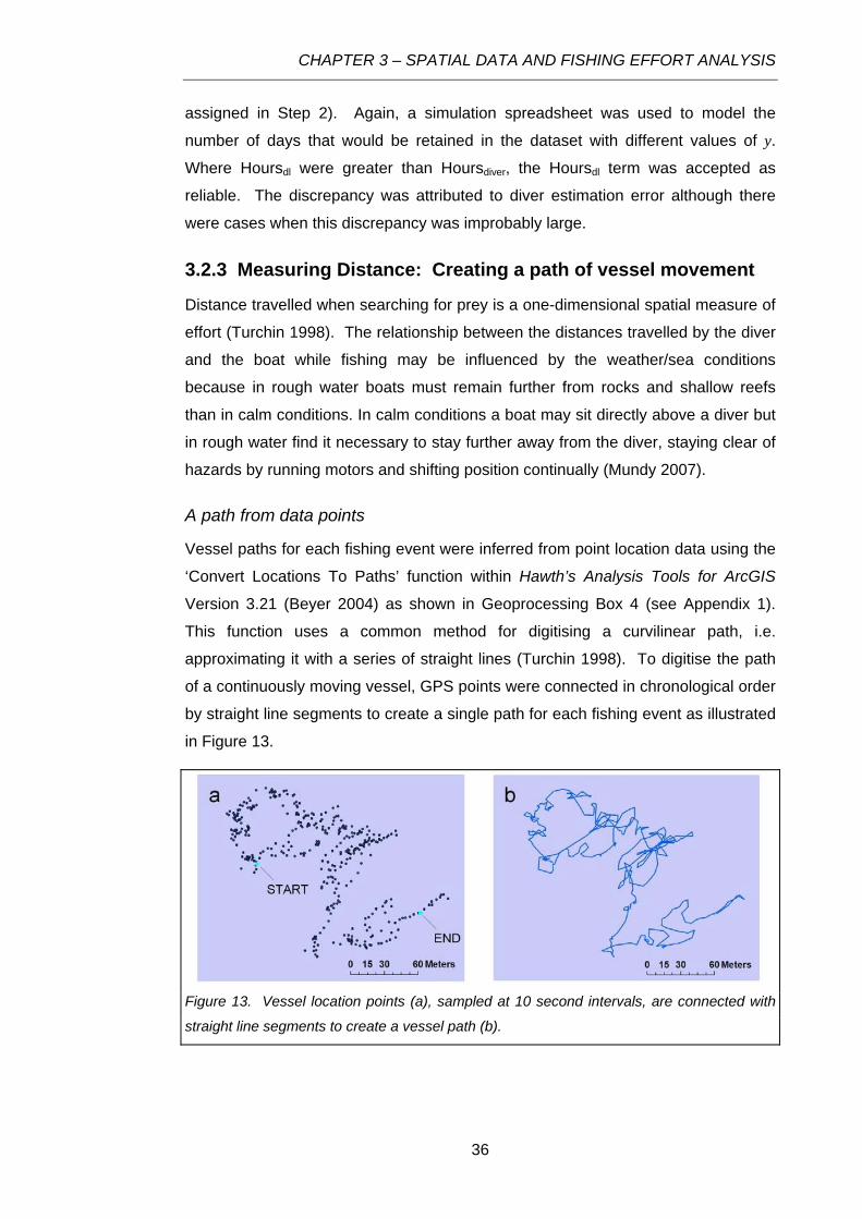
CHAPTER 3 – SPATIAL DATA AND FISHING EFFORT ANALYSIS
assigned in Step 2). Again, a simulation spreadsheet was used to model the
number of days that would be retained in the dataset with different values of y.
Where Hoursdl were greater than Hoursdiver, the Hoursdl term was accepted as
reliable. The discrepancy was attributed to diver estimation error although there
were cases when this discrepancy was improbably large.
3.2.3 Measuring Distance: Creating a path of vessel movement
Distance travelled when searching for prey is a one-dimensional spatial measure of
effort (Turchin 1998). The relationship between the distances travelled by the diver
and the boat while fishing may be influenced by the weather/sea conditions
because in rough water boats must remain further from rocks and shallow reefs
than in calm conditions. In calm conditions a boat may sit directly above a diver but
in rough water find it necessary to stay further away from the diver, staying clear of
hazards by running motors and shifting position continually (Mundy 2007).
A path from data points
Vessel paths for each fishing event were inferred from point location data using the
‘Convert Locations To Paths’ function within Hawth’s Analysis Tools for ArcGIS
Version 3.21 (Beyer 2004) as shown in Geoprocessing Box 4 (see Appendix 1).
This function uses a common method for digitising a curvilinear path, i.e.
approximating it with a series of straight lines (Turchin 1998). To digitise the path
of a continuously moving vessel, GPS points were connected in chronological order
by straight line segments to create a single path for each fishing event as illustrated
in Figure 13.
Figure 13. Vessel location points (a), sampled at 10 second intervals, are connected with
straight line segments to create a vessel path (b).
36

CHAPTER 3 – SPATIAL DATA AND FISHING EFFORT ANALYSIS
The frequency distributions of daily path distance for each diver were generated
and described. Paths of vessel movement were later used in buffer analyses
(section 3.2.4) and fishing behaviour analyses (Chapter 4).
Daily Catch Per Unit Distance
All vessel track lengths for a day were summed to give the total distance covered
during fishing by the vessel in that day, excluding travel between fishing events.
Catch per kilometre of vessel track (Catch Per Unit Distance) was calculated as:
CPUD = kg / km Eq. 4
Where kg is the daily catch in kilograms and km is the path length during fishing on
that day in kilometres. Fishing events of different durations create paths of different
lengths. The rate of movement (displacement through time) can be used to
standardise these paths with respect to time, however, as distance was here used
as a measure of effort in calculating CPUD, and daily catch was not standardised
for duration, this was not necessary.
3.2.4 Measuring Area: An index of diver ‘search’ area
The GPS loggers used in this study captured fine scale data by recording the
movement of the vessel used for fishing. Using vessel-mounted loggers meant that
the movement, or track, of a diver in the water was not recorded and the amount of
area searched by a diver was not measured exactly. The relationship between the
search patterns of a diver and the GPS path of a vessel was unknown, though likely
to be varied under a range of conditions. While the actual area searched by a diver
could not be determined using the data collected, standard GIS techniques were
used to calculate an estimate of the potential area utilised by the diver. This
estimate functioned as an index of diver search area.
Quantifying the area searched
The amount of area available to a diver to be fished during each fishing event was
estimated prior to generating a catch rate with a two dimensional spatial component
(catch per unit of area searched). Three different spatial analysis techniques were
37

CHAPTER 3 – SPATIAL DATA AND FISHING EFFORT ANALYSIS
applied to the data to calculate a range of area estimates that may describe diver
search area6. The techniques used were:
• Minimum Convex Polygon
• Buffer Analysis
• Kernel Density Analysis
Each technique was applied to data from individual fishing events to generate
descriptions of area available during each event. The differences between these
three measures of area search were tested using an ANOVA with repeated
measures. The area estimates were used to generate daily measures of catch per
unit of area (CPUA) searched. The values of CPUA from each technique were
compared using an ANOVA with repeated measures.
Minimum Convex Polygons
A minimum convex polygon (MCP) represents the minimum possible area
described by a convex polygon that contains a complete set of points. It can be
imagined as the area contained within a rubber band if it were stretched around the
outside, to contain all points in a set. Minimum Convex Polygons are frequently
used to generate home range estimates (Harris et al. 1990, Halloran and Bekoff
2000, Haenel et al. 2003), although they are not considered to be accurate in
estimating the use of space by an animal (Hooge et al. 1999, Halloran and Bekoff
2000). Using the Animal Movement tools created by Hawthorne Beyer for ArcGIS,
a minimum convex polygon was generated to contain all points that the working
vessel visited during each fishing event (Figure 14, Appendix 1: Geoprocessing Box
1). The area of each MCP was calculated using the ‘Add Area/Perimeter Fields To
Table’ function within Hawth’s Analysis Tools for ArcGIS Version 3.21 (Beyer 2004)
(Appendix 1: Geoprocessing Box 2).
6 The “potential area searched” is to be interpreted here as the area that the diver could
have sum over while looking for abalone, i.e. the potential range of places that the diver
could have been in. The definition does not consider underwater visibility (which varies from
day to day), field of vision, or habitat obstructions to line-of-sight.
38

CHAPTER 3 – SPATIAL DATA AND FISHING EFFORT ANALYSIS
Figure 14. Vessel location points (a) for a single fishing event are contained within a
Minimum Convex Polygon (b). The area of the polygon approximates the area searched by
the diver.
Buffer Analysis
All divers working in the Tasmanian abalone fishery breathe surface-supply
compressed air while they are fishing. Air is pumped by a low pressure compressor
on the vessel to the diver through a long 10 mm diameter hose (Figure 15) and the
deckhand maintains the vessel as close to the diver as weather conditions allow.
Pulling a long length of hose through the water requires exertion from a diver,
particularly when there is a current or strong wind at the water surface pulling the
hose in a direction other than that in which the diver is moving. A deckhand will
attempt to keep air hoses at a length allowing free movement of the diver but
reducing drag. Generally, less than 30 m of hose will be in the water during a dive,
but this is dependent on weather and sea conditions and diver preference (Mundy
2007).
Figure 15. Divers are tethered to a vessel by the surface supply compressed air hose
(yellow in these photographs). This diver is towing an orange surface buoy on a white line
so that his deckhand can find him easily. Credit: TAFI Abalone Group Image Collection,
2005.
39

CHAPTER 3 – SPATIAL DATA AND FISHING EFFORT ANALYSIS
In GIS, a buffer analysis generates a polygon of defined radius around a point,
collection of points or a line according to parameters outlined by the user of the
GIS. A buffer analysis can be used to define the possible search area of a diver
tethered to a vessel with an air hose of known length. By allowing a buffer radius of
30 m along the length of a dive track line (based on a reported average hose length
of abalone divers working in the Tasmanian Fishery) the maximum possible search
area of a diver can be identified (Figure 16). In reality a diver is likely to be within
30 m of the vessel for the majority of the dive. For example, while working at a
depth of approximately 20 m, a 30 m hose will not allow a diver to be much more
than 20 m from the vessel (Figure 17).
Figure 16. Maximum search area available is estimated from a vessel path (a) by buffering
to create a polygon containing all area within 30 m around the path (b).
40

CHAPTER 3 – SPATIAL DATA AND FISHING EFFORT ANALYSIS
VESSEL 30 m air hose at surface
30 m air hose at 30 m depth
45o
30 m
21.213 m
21.213 m
Figure 17. While working at a depth of approximately 20 m, a 30 m hose will not allow a diver
to be much more than 20m from the vessel.
Kernel Density Estimation
Kernel Density Estimation (KDE) is a probabilistic technique used for estimating the
home range of animals using a dataset of location points (Laver 2005). A Kernel
density estimation is a non-parametric density function because it does not assume
that data fit a prescribed distribution pattern, such as a circle (Selkirk and Bishop
2002). It has no shape assumption and is based on point density. Kernel density
estimation allows utilisation distribution to be established by drawing contours
around areas of equal density. Non-parametric methodologies are considered to
be the most successful of a variety of animal home range estimators (including the
MCPs described in section 3.2.4) (Worton 1989). For this reason a KDE of vessel
range during each fishing event was calculated.
Deriving a KDE is a multi-step process (Hooge et al. 1999, Beyer 2004, Laver
2005). A defined kernel (K) is placed over each point in a dataset, weighting the
area surrounding the point with values defined by the kernel function. Each point is
assigned a density value based upon the proximity of the point to other points in the
dataset within a defined radius. The smoothing parameter (h) describes the radius
41

CHAPTER 3 – SPATIAL DATA AND FISHING EFFORT ANALYSIS
and thus the search area around each point. A grid of defined cell size is placed
over the weighted point dataset and a density value is assigned to each grid cell
based upon the cumulative values of points contained in the cell. The grid surface
can be contoured at specified density thresholds to give percentage density surface
areas. Within GIS environments a range of tools have been developed to
automatically generate kernel density grids. These tools typically offer one or more
kernel types, a choice of statistically chosen or user-defined smoothing parameter
(h), and a choice of default or user-defined grid cell size.
For each fishing event in the dataset, KDEs were generated in ArcView 3.2 using
the Animal Movement Analysis ArcView extension (v2.04 beta) developed by P. N.
Hooge (Hooge 1998). A bivariate normal density kernel was used, with a
smoothing parameter, or ‘bandwidth’, of h = 10 and a grid cell size of 5 m. This
combination of smoothing value and grid cell size most closely matched the scale
of available data, leading to a balance between detail and resolution, i.e. not too
smooth and not too many holes. The kernel density grid surface was contoured at
95% and 50% density intervals to create polygons. Each contour represents
probability at a particular density, that is, the probability that the diver worked within
the contour at a particular time. Within the 95% density interval there is a 95%
probability that the diver was diving within that contour at any time during the fishing
event. These contours are illustrated in Figure 18. The 95% contour is here used
as an estimate of search area.
Figure 18. 95% of vessel location points (a) for a single fishing event are contained within
the 95% contour of a KDE raster surface (b).
42

CHAPTER 3 – SPATIAL DATA AND FISHING EFFORT ANALYSIS
Catch Per Unit Area
Each estimate of area available to a diver in a day was used to calculate kg/ha as a
Catch Per Unit of Area (CPUA) measure. For each fishing day of the year, the
areas of all vessel tracks were summed to give an estimate of daily total area
available to be searched by each diver, in hectares.
CPUA = kg / ha Eq. 5
Where kg is catch in kilograms and ha is the area available to be searched by each
diver in hectares.
3.2.5 CPUE and CPUA at a fine spatial scale
One catch rate for multiple fishing events
In sections 3.2.1 to 3.2.4, catch rate values were calculated for each day of fishing
activity. On most of these days, multiple fishing events had occurred. Three
methods were considered for allocating catch rates to these fishing events:
A. Identify the management blocks in which all fishing events for each day of
fishing occurred, and allocate a catch rate to those blocks.
B. Create a MCP (see section 3.2.4 ‘Minimum Convex Polygons’ for methods)
that encompasses all fishing events for a day of fishing, and allocate a catch
rate to the polygon.
C. Identify every fishing event that contributed to a day’s catch and allocate the
same catch rate (in kg/hr) to each of those individual fishing events.
The first method (A) is at the coarse spatial scale of current CPUE estimates.
Method B is at a much finer spatial scale than A; each polygon encompasses all
fishing events that contribute to the day’s catch rate. However, the polygons also
encompass area that was not fished. Method C identifies the fishing locations that
contributed to a day’s catch rate and doesn’t include obviously unfished area.
CPUE estimates are allocated to the fishery at the spatial scale of single fishing
events, with mean catch rates calculated for whole days of fishing activity. Method
C was chosen to allocate daily CPUE and spatial catch rates to the fishery at as
fine a spatial scale as possible.
Allocating catch rates to each fishing event
The centroid location of each fishing event was mapped using ArcGIS. All fishing
events that contributed to each day of fishing were assigned to the diver’s catch
43

CHAPTER 3 – SPATIAL DATA AND FISHING EFFORT ANALYSIS
rate for that day. Thus, if a daily catch rate of 100 kg/hr was derived from three
different dives (fishing events), then each of the three events was assigned a
pooled catch rate of 100kg/hr. The centroid coordinates were linked to the CPUEdl,
CPUD, CPUA and other spatial descriptive statistics of that fishing event.
CPUEdl, CPUD and CPUA for each fishing event were plotted on a map of the
Tasmanian abalone fishery. These data can be aggregated at any spatial or
temporal scale desired to deliver fishery performance measures.
Summary of catch rate indices
In this chapter, four different catch rate measures were developed for each day of
fishing (Table 3
Table 3. Summary of the catch rate indices generated in chapter 3.
). These measures were CPUEdiver, the traditional catch per hour
used in management of the Tasmanian abalone fishery (kg.hr-1); CPUEdl, a more
accurate catch per hour generated from dive logger data (kg.hr-1); CPUD, a
measure of catch per kilometre of vessel track (kg.km-1); and CPUA, an index of
catch per hectare generated from an estimate of search area available to the diver
(kg.ha-1). Separate catch rates were not generated for individual fishing events
because catch data were only available for each day of fishing.
Catch Per Unit of Effort
Effort measure
Units of effort
Source Scale of data collection
Scale of data aggregation
Time Hours Reported by diver
Day Day CPUEdiver (of fishing)
Time Hours Recorded by depth logger
Fishing Event Day CPUEdl (of fishing)
Distance Kilometres Length of calculated vessel path
Fishing Event Day CPUD (travelled)
Area Hectares Contained in the 95% density contour of a kernel density estimate
Fishing Event CPUA (potentially searched)
Day
Catch rates (CPUEdiver, CPUEdl, CPUD and CPUA) were calculated for 149
separate days of fishing effort across all three divers (A, B and C). These catch
rates were allocated to a total of 628 individual fishing events (Table 4, compare
with Table 2 in Chapter 2). 64% of all fishing events recorded by Divers A, B and C
between July 2005 and April 2007 were assigned catch rates.
44
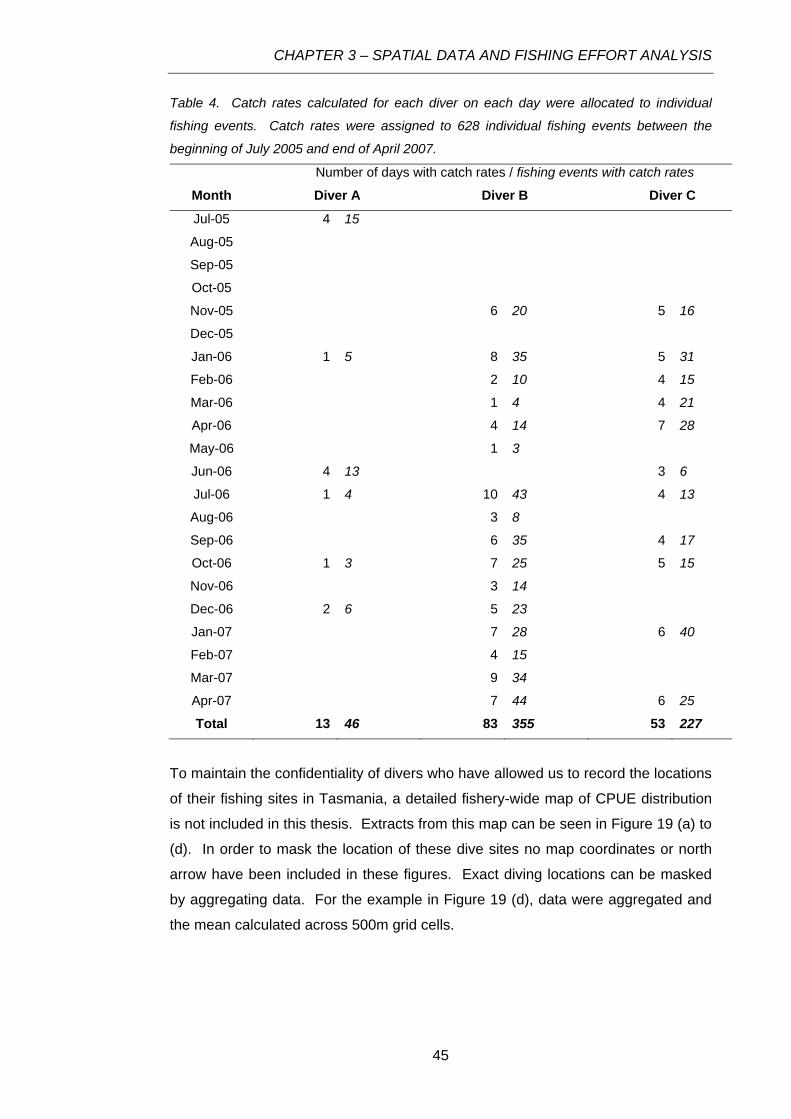
CHAPTER 3 – SPATIAL DATA AND FISHING EFFORT ANALYSIS
Table 4. Catch rates calculated for each diver on each day were allocated to individual
fishing events. Catch rates were assigned to 628 individual fishing events between the
beginning of July 2005 and end of April 2007.
Number of days with catch rates / fishing events with catch rates
Month Diver A Diver B Diver C
Jul-05 4 15
Aug-05
Sep-05
Oct-05
Nov-05 6 5 20 16
Dec-05
Jan-06 1 8 55 35 31
Feb-06 2 4 10 15
Mar-06 1 4 4 21
Apr-06 4 7 14 28
May-06 1 3
Jun-06 4 313 6
Jul-06 1 10 44 43 13
Aug-06 3 8
Sep-06 6 4 35 17
Oct-06 1 7 53 25 15
Nov-06 3 14
Dec-06 2 5 6 23
Jan-07 7 6 40 28
Feb-07 4 15
Mar-07 9 34
Apr-07 7 44 6 25
Total 13 46 83 355
53 227
To maintain the confidentiality of divers who have allowed us to record the locations
of their fishing sites in Tasmania, a detailed fishery-wide map of CPUE distribution
is not included in this thesis. Extracts from this map can be seen in Figure 19 (a) to
(d). In order to mask the location of these dive sites no map coordinates or north
arrow have been included in these figures. Exact diving locations can be masked
by aggregating data. For the example in Figure 19 (d), data were aggregated and
the mean calculated across 500m grid cells.
45

CHAPTER 3 – SPATIAL DATA AND FISHING EFFORT ANALYSIS
!(
!(
!(
!(
!(
CPUE: 92 kg/hr
CPUE: 55 kg/hr
CPUE: 55 kg/hrCPUE: 94 kg/hr CPUE: 111 kg/hr!(
!(
!(
!(
!(
CPUD: 60 kg/km
CPUD: 46 kg/km
CPUD: 46 kg/kmCPUD: 61 kg/km CPUD: 136 kg/km
!(
!(
!(
!(
!(
CPUA: 59 kg/ha
CPUA: 48 kg/ha
CPUA: 48 kg/haCPUA: 61 kg/ha CPUA: 171 kg/ha
a b
c d
!(
!(
!(
!(
!(
CPUE: 92 kg/hr
CPUE: 55 kg/hr
CPUE: 55 kg/hrCPUE: 94 kg/hr CPUE: 111 kg/hr!(
!(
!(
!(
!(
CPUD: 60 kg/km
CPUD: 46 kg/km
CPUD: 46 kg/kmCPUD: 61 kg/km CPUD: 136 kg/km
!(
!(
!(
!(
!(
CPUA: 59 kg/ha
CPUA: 48 kg/ha
CPUA: 48 kg/haCPUA: 61 kg/ha CPUA: 171 kg/ha
a b
c d
Figure 19. Extracts from a map showing every fishing event to which catch rates were allocated.
CPUE (kg/hr) (a), CPUD (kg/km) (b) and CPUA (kg/ha) (c) estimates were calculated daily and
allocated to all fishing events that contributed to the day’s catch. A 500m grid was imposed on
the map. CPUE estimates were aggregated and the mean calculated across grid cells (d).
Values were colour coded: Dark green: 0-40 kg/hr, Mid-green:40-80 kg/hr, Light green: 80-120
kg/hr.
3.2.6. Testing the differences between the different indices: across all divers and for each diver
I applied statistical tests to the different measures of effort (e.g., duration of a
fishing event, or distance covered by the vessel while fishing) and catch-rate
indices (i.e., CPUE, CPUD, CPUA). Statistical tests presented in the following
sections were computed using the R software (R version 2.8.1. Copyright: The R
Foundation for Statistical Computing) for statistics.
Analyses of measures of fishing time (Hoursdiver; Hoursdl)
Firstly, using fishing time as measured by data loggers, I focus on the effect of
imprecise reporting of fishing time by diver as a source of error. To consider error in
time reporting, a Two-way ANOVA was performed on fishing time estimates using
46

CHAPTER 3 – SPATIAL DATA AND FISHING EFFORT ANALYSIS
‘method’, i.e., Hoursdiver (as reported by the diver) and Hoursdl (as measured by the
data logger) and ‘diver’ as factors.
Analyses of distance-based catch-per-unit-of-effort (CPUD)
An ANOVA was performed with CPUD as the dependent variable and ‘diver’ (A, B
or C) as a factor to test for differences in CPUD between divers.
Analyses of area-based catch-per-unit-of-effort (CPUA)
A two-way ANOVA on area-based catch-rates was performed with ‘method’ (the
three different area-based indices of abundance: CPUAmcp based on a Minimum
Convex Polygon, CPUAbuf based on a buffered vessel track and CPUAkde the 95%
density contour from a Kernel Density Estimate) and ‘diver’ as factors, including
interactions between method and diver.
To stabilise residual deviance when needed, some of the response variables were
transformed (log-transformed, or square-root transformed). Results of statistical
tests are presented on untransformed data, when transformations did not affect the
significance of the results (see Appendix 4). Box-Cox tests were performed using
the R function of the same name (‘boxcox’).
3.3 Results
Each whole day of fishing was treated independently in these analyses. This
forced level of aggregation was caused by the scale of catch-reporting and is in
contrast to the analyses in Chapter 4 where each fishing event was treated
independently.
3.3.1 Measuring time: disparities between logger recorded and diver reported dive times?
Duration of fishing activity
Fishers frequently reported their estimates of total fishing time imprecisely, in whole
hour and half hour blocks. Occasionally one diver reported fishing time to the
nearest 15 minutes (Figure 20).
Diver estimates of daily fishing effort duration were not always close to time
recorded by loggers (Figure 21). The mean difference was an overestimate of
5.3% of fishing time reported by a diver relative to the time measured by the data
47

CHAPTER 3 – SPATIAL DATA AND FISHING EFFORT ANALYSIS
logger. This difference was due to a combination of diver error and depth logger
error. Diver ’overestimates’ are shown in Figure 21 as negative discrepancies.
Visual inspection of the data in Figure 20 and Figure 21 indicates that Diver A
almost consistently reported an estimated fishing time higher than that measured
by the logger. Across all divers, an ‘overestimate’ of fishing time was more frequent
(72% of all fishing days) than an ‘underestimate’.
0
1
2
3
4
5
6
7
8
9
0 2 4 6 8
Diver A n = 62
Diver B n = 106
Diver C n = 78
Hou
rsdi
ver
Hoursdl
Figure 20. Relationship between fishing time estimated by divers (Hoursdiver) and fishing
time recorded by the depth loggers (Hoursdl). If depth logger values were correct, diver
estimates would be both inaccurate and imprecise. An perfect diver estimate would fall on
the red line (i.e. Hoursdiver = Hoursdl).
48

CHAPTER 3 – SPATIAL DATA AND FISHING EFFORT ANALYSIS
5
10
15
20
25
30
35
Cou
nt
-250 -220 -200 -180 -160 -140 -120 -100 -80 -60 -40 -20 0 10 30 50 70 90 110 130 150 170 190
Hours dl - Hours diver (discrepency in min)
Figure 21. Frequency distribution of the discrepancy (minutes) between fishing time recorded
by depth loggers (Hoursdl) and fishing time estimated by divers (Hoursdiver).
However, during preliminary exploration of time data pooled across all divers (226
observations; see Figures 20 and 21), investigation of outliers, i.e., extreme values
of discrepancy between CPUEdl and CPUEdiver revealed malfunctions in the
equipment used to collect fishing time data, in addition to the imprecision in fishing
time that was reported by divers. Note that the presence of some extreme
differences between the two indices reflect either inaccurate depth logger data due
to equipment malfunction, or may also have occurred when divers did not wear the
logger for all dives during a fishing day. Raw data were filtered to remove these
erroneous data records. The next section of this chapter describes the filtering
process of the raw data.
3.3.2 Selecting Days for Spatial Catch Rate Analyses
Step 1 of Data Exclusion Algorithm
Across all divers, the disparity between Hoursdl and HoursGPS ranged between 0
and 445 minutes in a day. At 0 minutes no spatial data were missing from the day’s
effort dataset. At 445 minutes almost 7.5 hours of fishing had been recorded by
that dive logger, for which no spatial data were collected. The distribution of
disparity between Hoursdl and HoursGPS was different for each of Diver A, B and C
but for all divers this disparity was most often <10 minutes: 75% of days with depth
logger data for Diver B (n = 106), 53% for Diver C (n = 78) and 28% for Diver A (n =
65).
49

CHAPTER 3 – SPATIAL DATA AND FISHING EFFORT ANALYSIS
In Figure 22, x is plotted as an accepted disparity between Hoursdl and HoursGPS.
Up to 10% disparity in dive duration between the two data sources (x = 0.1) was
considered acceptable (i.e. 10% of depth logger recorded fishing activity had no
matching GPS data). Retention in step 1 was 32% for Diver A, 80% for Diver B and
69% for Diver C. This trade-off between data quantity and quality was necessitated
by problems encountered in data collection (see Chapter 2) and balanced the
exclusion of days with lots of GPS data missing with a desire to retain a dataset of
sufficient size for analysis.
0
10
20
30
40
50
60
70
80
90
100
0 0.1 0.2 0.3 0.4 0.5 0.6 0.7 0.8 0.9 1
Accepte
Step 2 of Data Exclusion Algorithm
In Figure 23 the accepted error in diver estimate (y) is modelled as the ‘error’ in
diver estimates of dive duration (Hoursdiver) compared to dive duration measured by
depth logger (Hoursdl). This step excluded days when a diver estimate of dive
duration was much greater than the measured duration, indicating that some diving
may have gone unlogged by both the GPS and depth/temperature data loggers. y
was limited to ≤ 30%. At the (Hoursdl+30%) exclusion rate, retention in step 2 was
62.5% for Diver A, 97.5% for Diver B and 97.6% for Diver C (see Table 5 for
details). The percentage of days retained in the dataset reached a plateau or near-
plateau for divers A and B when a +30% error acceptance rate was applied (vertical
dotted line). Diver C was an exception (cf Figure 24).
d disparity (as a proportion of Hoursdl)
% d
ays
reta
ined
Diver A
Diver B
Diver C
Figure 22. Step 1 of the exclusion algorithm: Modelling the effects of different values of
accepted disparity (as a proportion of Hoursdl) on data retention. The vertical dotted line
illustrates the outcome when the disparity is equal to or less than 10% of Hoursdl.
Disparity
50
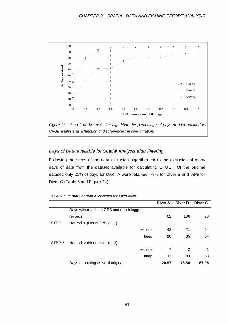
CHAPTER 3 – SPATIAL DATA AND FISHING EFFORT ANALYSIS
0
10
20
30
40
50
60
70
80
90
100
0 0.1 0.2 0.3 0.4 0.5 0.6 0.7 0.8 0.9 1
Accepte r (proportion of Hoursdl)
% d
ays
reta
ined
Diver A
Diver B
Diver C
d erro
Figure 23. Step 2 of the exclusion algorithm: the percentage of days of data retained for
CPUE analysis as a function of discrepencies in dive duration.
Days of Data available for Spatial Analysis after Filtering
Following the steps of the data exclusion algorithm led to the exclusion of many
days of data from the dataset available for calculating CPUE. Of the original
dataset, only 21% of days for Diver A were retained, 78% for Diver B and 68% for
Diver C (Table 5 and Figure 24).
Table 5. Summary of data exclusions for each diver.
Diver A Diver B Diver C
Days with matching GPS and depth logger
records 62 106 78
STEP 1 Hoursdl > (HoursGPS x 1.1) exclude 42 21 24
keep 20 85 54STEP 2 Hoursdl > (Hoursdiver x 1.3) exclude 7 2 1
keep 13 83 53 Days remaining as % of original 20.97 78.30 67.95
Error
51

CHAPTER 3 – SPATIAL DATA AND FISHING EFFORT ANALYSIS
Diver A
0
1
2
3
4
5
6
7
8
9
0 1 2 3 4 5 6 7 8
Hoursdl
Hou
rsdi
ver
9
Exclude Step 1Exclude Step 2KeepHoursdiver = Hoursdl(Hoursdl*1.3) exclusion line
Figure 24a. Days of data kept following the data exclusion algorithm (shown in orange) for
Diver A. Points falling above the blue line were excluded at a +30% exclusion rate in step 2
(cf Figure 23). An accurate diver estimate (Hoursdiver equal Hoursdl) falls on the red line when
the depth logger captured all dive data (i.e. was deployed on all dives for a day).
Diver B
0
1
2
3
4
5
6
7
8
9
0 1 2 3 4 5 6 7 8 9
Hoursdl
Hou
rsdi
ver
Exclude Step 1Exclude Step 2KeepHoursdiver = Hoursdl(Hoursdl*1.3) exclusion line
Figure 24b. Days of data kept following the data exclusion algorithm (shown in orange) for
Diver B.
52

CHAPTER 3 – SPATIAL DATA AND FISHING EFFORT ANALYSIS
Diver C
0
1
2
3
4
5
6
7
8
9
0 1 2 3 4 5 6 7 8Hoursdl
Hou
rsdi
ver
9
Exclude Step 1Exclude Step 2KeepHoursdiver = Hoursdl(Hoursdl*1.3) exclusion line
Figure 24c. Days of data kept following the data exclusion algorithm (shown in orange) for
Diver C.
All results presented hereafter are derived from analyses performed on the filtered
data set.
Effect of error in time reporting on daily CPUE
Using the filtered data, the mean absolute discrepancy between Hoursdiver and
Hoursdl was significantly different to 0 (F1,146=121.47 - P inferior to 0.0001) and
consistent across all divers (F2,146=0.60; P = 0.5489).
Both inaccuracy and imprecision in diver’s effort estimates are reflected in the
discrepancies between CPUEdiver and CPUEdl (Figure 25). Note that CPUE data,
as plotted in Figure 25, also reflects any errors in catch data, but misreporting of
catch data is outside the scope of this study.
The ANOVA reveals that individual divers (A, B or C) have a significant effect on
mean CPUE values (F2,292=6.7028; P=0.001425), while there was no difference
between the two CPUE methods (F1,292= 0.0338; P= 0.854) and nor is there an
interaction between diver and method (F2,292=0.0401; P=0.9607).
53

CHAPTER 3 – SPATIAL DATA AND FISHING EFFORT ANALYSIS
Figure 25. Frequency distribution of CPUE estimates for each method (CPUEdiver and CPUEdl)
and individual diver (A, B or C).
3.3.3 Measuring Distance: Creating a path of vessel movement
Across all divers, daily summed path lengths ranged from 1.2 km to 15.4 km (n =
147). For diver A , the mean daily path length was 6.1 km, for Diver B it was 5.2 km
and for Diver C it was 7.9 km (see Table 6
Table 6. The sum of path lengths (m) for each. One outlier was excluded from datasets for
each of Diver B and Diver C.
for a summary).
Diver A Diver B Diver C
6061.65 5191.33 7947.67Mean Std Dev 1990.49 2251.99 2938.94
552.06 248.69 407.56Std Err Mean 7264.50 5686.15 8765.87upper 95% Mean 4858.81 4696.52 7129.46lower 95% Mean
54

CHAPTER 3 – SPATIAL DATA AND FISHING EFFORT ANALYSIS
N 13 82 52
Daily Catch per Unit of Distance
For each day of catch in the filtered dataset a value of catch per unit of distance
(CPUD) was calculated Figure 25). Results from the analyss of variance suggest
that ‘diver’ has a significant effect on CPUD estimates (F2,143=15.77; P=6e-07).
Comparison of CPUD for Diver C and Diver B reveals very different foraging
strategies between the two fishers: Diver B intensively harvests individuals along
the distance covered relative to Diver C, who appears to be covering longer
distances to achieve a similar CPUEdl.
The small sample size here means that future investigations would be required
across a wider proportion of the fishery to further explore the use of the relationship
between CPUD and time-based CPUE to characterise different harvesting
strategies.
Figure 25. Frequency distribution of catch per unit of distance CPUD (kg/km) for each of three
divers A, B and C.
55

CHAPTER 3 – SPATIAL DATA AND FISHING EFFORT ANALYSIS
3.3.4 Measuring Area: An index of diver ‘search’ area
Three estimates of available search area were generated for every fishing event: a
Minimum Convex Polygon (Amcp), a buffered vessel track (Abuf) and the 95% density
contour from a Kernel Density Estimate (Akde). For each diver, area estimates of
single fishing events were summed across a day to calculate a potential daily
search area. There were some significant differences in CPUA indices between
divers (ANOVA: F2,438= 10.9549; P=2.278e-05) and between methods of estimating
potential search area (ANOVA: F2,438= 64.9128; P< 2.2e-16). See Table 11 in
Appendix 4 for posthoc comparisons. Abuf estimates were approximately twice the
area of Akde estimates. Akde was almost consistently the lowest estimate and Abuf the
highest (Figure 26).
35
0
5
10
15
20
25
30
Abuf Akde Amcp
Pote
ntia
l dai
ly s
earc
h ar
ea (H
a)
35
0
5
10
15
20
25
30
Abuf Akde Amcp
Pote
ntia
l dai
ly s
earc
h ar
ea (H
a)
Figure 26. Distribution plots of estimated potential daily diver search area, for all divers,
calculated with three techniques: MCP (Amcp), buffer (Abuf) and KDE 95% contour (Akde). The
three area estimates are significantly different from each other (Student’s t-test P = 0.05).
Green diamonds mark Mean and Standard Error for each distribution.
56
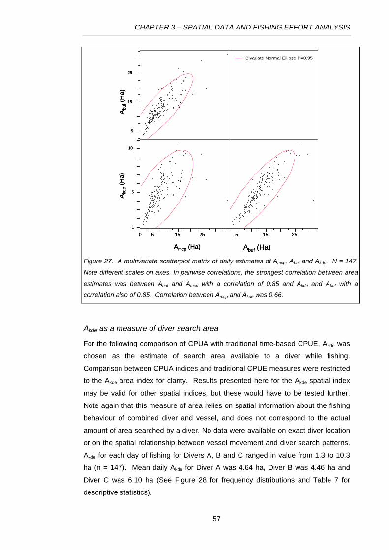
CHAPTER 3 – SPATIAL DATA AND FISHING EFFORT ANALYSIS
Akde as a measure of diver search area
For the following comparison of CPUA with traditional time-based CPUE, Akde was
chosen as the estimate of search area available to a diver while fishing.
Comparison between CPUA indices and traditional CPUE measures were restricted
to the Akde area index for clarity. Results presented here for the Akde spatial index
may be valid for other spatial indices, but these would have to be tested further.
Note again that this measure of area relies on spatial information about the fishing
behaviour of combined diver and vessel, and does not correspond to the actual
amount of area searched by a diver. No data were available on exact diver location
or on the spatial relationship between vessel movement and diver search patterns.
Akde for each day of fishing for Divers A, B and C ranged in value from 1.3 to 10.3
ha (n = 147). Mean daily Akde for Diver A was 4.64 ha, Diver B was 4.46 ha and
Diver C was 6.10 ha (See Figure 28 for frequency distributions and Table 7 for
descriptive statistics).
Amcp (Ha)
A kde
(Ha)
Abu
f(H
a)
Abuf (Ha)
5
15
25
1
5
10
0 5 15 25 5 15 25
Bivariate Normal Ellipse P=0.95
Amcp (Ha)
A kde
(Ha)
Abu
f(H
a)
Abuf (Ha)
5
15
25
1
5
10
0 5 15 25 5 15 25
Amcp (Ha)
A kde
(Ha)
Abu
f(H
a)
Abuf (Ha)
5
15
25
1
5
10
0 5 15 25 5 15 25
Bivariate Normal Ellipse P=0.95
Figure 27. A multivariate scatterplot matrix of daily estimates of Amcp, Abuf and Akde. N = 147.
Note different scales on axes. In pairwise correlations, the strongest correlation between area
estimates was between Abuf and Amcp with a correlation of 0.85 and Akde and Abuf with a
correlation also of 0.85. Correlation between Amcp and Akde was 0.66.
57

CHAPTER 3 – SPATIAL DATA AND FISHING EFFORT ANALYSIS
2
6
10
Cou
nt
0 0.5 1 1.5 2 2.5 3 3.5 4 4.5 5 5.5 6 6.5 7 7.5 8 8.5 9 9.5 10 11
12
3
Cou
nt
0 0.5 1 1.5 2 2.5 3 3.5 4 4.5 5 5.5 6 6.5 7 7.5 8 8.5 9 9.5 10 11
1357
Cou
nt
0 0.5 1 1.5 2 2.5 3 3.5 4 4.5 5 5.5 6 6.5 7 7.5 8 8.5 9 9.5 10 11
a
b
c
Diver A Daily Akde
Diver B Daily Akde
Diver C Daily Akde
Figure 28. Frequency distribution of Akde (ha) for each day, for each of Divers A (a), B (b), and
C (c). Note the different scales on the y-axes. Quantile box plots for each distribution are
given. Cf Table 7.
58

CHAPTER 3 – SPATIAL DATA AND FISHING EFFORT ANALYSIS
Table 7. Descriptive statistics for the frequency distributions of Akde (ha) for Divers A, B and C. Cf.
Figure 28.
Diver A Diver B Diver C
Mean 4.640 4.463 6.104
Std Dev 1.257 1.888 1.798
Std Err Mean 0.349 0.208 0.249
5.400 4.878 6.604upper 95% Mean 3.881lower 95% Mean 4.048 5.603
N 13 82 52
Daily Catch Per Unit of Area (CPUA)
For each diver and each day of fishing, the catch rate per unit of area (CPUA) was
calculated in kg/Ha. There were some significant differences in CPUA values
between methods of estimating potential search area (ANOVA: F2,438= 14.570; P<
7.5e-7). The effect of individual divers was not significant (F2,438= 1.171; P=0.311).
The three area-based CPUE estimate perform differently to each other.
A visual inspection of the relationships between catch per unit of area (CPUA)
using the three different estimates of searched area against traditional time-based
CPUE (CPUEdl) was performed for each fishing day and per diver (Figure 30).
These plots illustrate the divergence in the different area-based indices of CPUE.
Similarly to the relationship between time-based CPUE and distance-based CPUD
(cf. previous sections), it would be worthwhile investigating the relationship between
CPUA and CPUE as a measure to characterise individual fishing behaviour. In
terms of fine-scale monitoring of fishing activity, it would be particularly relevant to
test whether some ‘types’ of harvesting behaviours defined using these indices
consistently emerge across divers of the Tasmanian abalone fishery. The small
sample size did not allow for such investigation in this study.
59

CHAPTER 3 – SPATIAL DATA AND FISHING EFFORT ANALYSIS
(a)
(b)
(c) Figure 29. Catch per unit of area (kg.ha-1) derived from Amcp (a), Abuf (b) and Akde (c) plotted
against CPUE (kg.hr-1) for each of three divers A (solid blue dots), B (solid red dots) and C
(black diamonds). Similar x and y scales are used to facilitate visual comparison.
60

CHAPTER 3 – SPATIAL DATA AND FISHING EFFORT ANALYSIS
3.4 Case Study: using spatial indices to standardise catch
rates
This case study focuses on the diver identified as “Diver A”. I have previously
discussed the differences between the alternative measures developed to estimate
catch rate across all divers. Here, I focus on demonstrating the different
standardised spatial indices that I have developed in Chapter 3, using 13 fishing
days of data recorded by Diver A.
To rank the quality of the different abundance indices would require specific
knowledge about actual abundance of abalone in the study area. Instead, this
section aims to illustrate the effects of the different standardisations of fishing effort
on catch rate estimates. Standardisation could reduce and would ideally eliminate
the effects on catch rate of different fishing gear, fisher experience and fishing
habitat (Haddon 2001). Because divers differ in their performance, as measured by
CPUE, CPUD and CPUA, such catch rate measures should be standardised when
used as an index of abundance. Catch rate improves as a measure of abundance
after standardisation. In the Tasmanian abalone fishery, diver catch rate
standardisation is performed using a combination of factors including diver, season
(month) and location (statistical block) (Tarbath et al. 2007). A measure of effort
distribution could improve standardisation of catch rate when it is used for
assessment. Currently, it is possible for CPUE to remain constant while the spatial
distribution of effort changes. A precise measure of effort distribution in space and
time such as area or distance covered while fishing should improve the spatial
distinction of effort.
This case study focuses on the fishing effort of one diver working the Actaeon Reef
in southeast Tasmania between January 2006 and April 2007. Thirty-one dives
over 13 days of fishing provided data for 8 catch rate estimates, after 5 days were
excluded from analysis during data filtering (Figure 30 and Table 8).
61
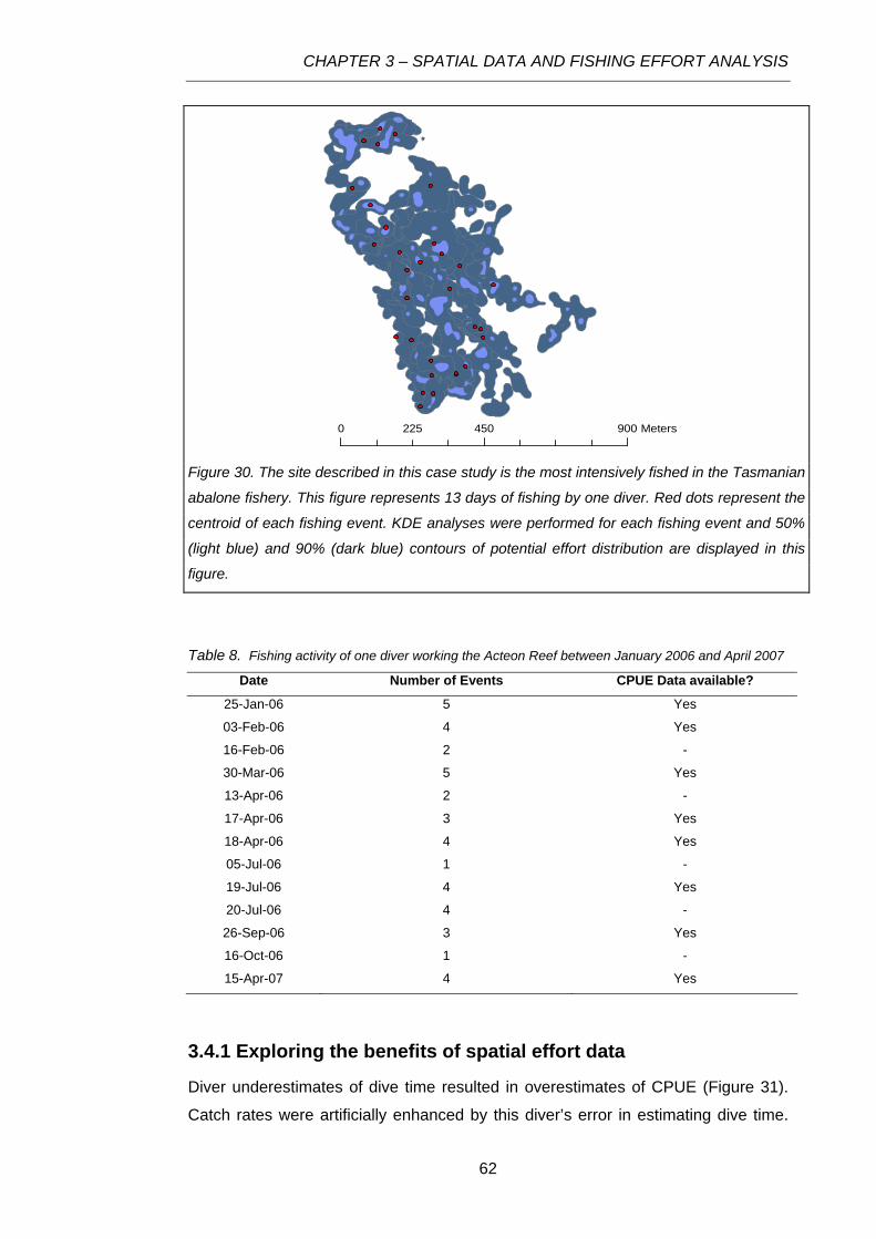
CHAPTER 3 – SPATIAL DATA AND FISHING EFFORT ANALYSIS
0 450 9225 Meters
Table 8. Fishing activity of one diver working the Acteon Reef between January 2006 and April 2007
3.4.1 Exploring the benefits of spatial effort data
00
Figure 30. The site described in this case study is the most intensively fished in the Tasmanian
abalone fishery. This figure represents 13 days of fishing by one diver. Red dots represent the
centroid of each fishing event. KDE analyses were performed for each fishing event and 50%
(light blue) and 90% (dark blue) contours of potential effort distribution are displayed in this
figure.
Date Number of Events CPUE Data available?
25-Jan-06 5 Yes
03-Feb-06 4 Yes
16-Feb-06 2 -
30-Mar-06 5 Yes
13-Apr-06 2 -
17-Apr-06 3 Yes
18-Apr-06 4 Yes
05-Jul-06 1 -
19-Jul-06 4 Yes
20-Jul-06 4 -
26-Sep-06 3 Yes
16-Oct-06 1 -
15-Apr-07 4 Yes
Diver underestimates of dive time resulted in overestimates of CPUE (Figure 31).
Catch rates were artificially enhanced by this diver’s error in estimating dive time.
62

CHAPTER 3 – SPATIAL DATA AND FISHING EFFORT ANALYSIS
Using the area of the 95% KDE contour rather than distance as a spatial measure
appears to eliminate some movement of the vessel that is not associated with diver
movement (Figure 31).
Figure 31. Association between CPUE (diver estimated time) and measures of Catch Per
spatial Unit of effort using data recorded by the logger (hr, ha, km). a) CPUEdiver against
CPUEdl. b) Measures of effort that include spatial distribution based upon units of area
(CPUA) or of distance (CPUD). Each measure of effort that includes spatial distribution
gives a different pattern of catch rate relative to the traditional CPUE.
CPU
Akd
e (kg
.ha-1
)
CPU
E dl (
kg.h
r-1)
CPU
D (k
g.km
-1)
CPUEdiver (kg.hr-1)
CPUEdl (kg.hr-1)
b
a
63

CHAPTER 3 – SPATIAL DATA AND FISHING EFFORT ANALYSIS
By looking at the relationship between catch, time, and area covered while fishing,
spatial measures of effort can be incorporated into interpretations of catch rate.
Fishing search rate can be calculated as the estimated amount of ‘area fished’ by a
diver (derived from GPS data) in a unit of time to give a search rate in hectares per
hour (CPUA) (see section 3.2.4 ‘Catch Per Unit Area’ for methods). For this case
study, Search Rate (Ha/hr) was plotted against catch rate (CPUE in Kg/Hr) (Figure
32).
Including spatial data in measures of fishing effort identifies two separate activities
that involve time; primarily searching for abalone and primarily handling abalone. In
Figure 32 two patterns of behaviour identify two types of effort distribution. When
traditional catch rates are high (above 90 Kg/hr) then the diver can be considered to
be exhibiting “fishing” behaviour. CPUE may be limited by ‘handling time’ and not
‘search time’. When traditional catch rates are low (below 90 Kg/hr) then more
searching behaviour is seen. There is a strong negative correlation between
search rate (in Ha/hr) and catch rate. When the diver is swimming and covering
area, they are not catching a lot of abalone.
64

CHAPTER 3 – SPATIAL DATA AND FISHING EFFORT ANALYSIS
65
3.4.2 Conclusions
Data loggers enable researchers to collect large amounts of data, however,
rigorous attention to collecting good quality data is important as poor quality data
are necessarily discarded from datasets. The site described here is the most
intensely fished in the Tasmanian abalone fishery. Plotting search rate (ha/hr)
against CPUE (kg/hr) for this site has identified a threshold at which fishing
behaviour appears to change from ‘searching’ (swimming and covering area) to
‘fishing’ (little area is covered and catch rate is high). It could be very valuable to be
able to easily categorise different patterns of diver distribution of effort between
fishing (handling) and searching activities. If a change in fishing behaviour can
consistently be identified by the relationship of CPUA to CPUE then it might be
used to standardise for effort during data filtering.
y = 0.0025x + 0.9519R2 = 0.9982
y = -0.0445x + 5.3079R2 = 0.8327
1
1.1
1.2
1.3
1.4
1.5
1.6
1.7
1.8
1.9
2
75 80 85 90 95 100 105 110 115
Traditional CPUE (Kg/Hr)
Sea
rch
Rat
e C
PU
A (H
a/H
r)
Figure 32. Eight data points derived from the 13 days of fishing activity illustrated in the map
in Figure 30. There is a negative correlation between search rate and catch rate up to a
threshold catch rate (Kg/Hr). Above the threshold, search rate is almost constant despite
increasing catch rates.

CHAPTER 3 – SPATIAL DATA AND FISHING EFFORT ANALYSIS
3.5 Discussion
3.5.1 Efficacy of electronic methods for effort capture
Improving measurements of effort
Using depth loggers to record fishing duration can potentially improve CPUE
estimates by providing a convenient means of accurately measuring the duration of
fishing activity for each day of fishing. Divers regularly round their estimates of
fishing time spent to the nearest half hour, with the estimates reported to DPIW
being approximate and often inaccurate. Divers do not necessarily refer to a dive
computer when recording catch and effort details at the end of a day’s fishing,
which may contribute to the inaccuracy. Historically, a reported ‘best guess’
estimate of time spent fishing has been considered sufficient by fishery managers
and researchers (Tasmanian Abalone Council Ltd 2002). Nevertheless, this study
suggests a significant absolute difference between time reported by divers and
measured by depth loggers. On average in this study, divers appeared to
overestimate the amount of time they spent fishing, most frequently by 0-10
minutes (see Figure 21), but the sign of the error (i.e., over- or under-estimate)
significantly varied between individual divers. Importantly, failure to wear depth
loggers while diving was flagged as a cause of apparent overestimate of dive time,
(Section 3.5.1).
Effects of improved effort measurement on CPUE
Errors in time estimate did not significantly affect CPUE estimates for the three
divers who participated in this study. However, further investigations using more
reliable time data collection across a wider proportion of the Tasmanian abalone
fishery would be essential to confirm these results. Consistent errors in dive time
estimation by just a few divers in the fishery may be enough to artificially inflate or
deflate catch rates calculated from diver estimated fishing durations. This would
affect fishery-wide catch rates as they are currently calculated. Note that
inaccurate reporting of catch data by divers (see Section 3.3.1 ‘Daily CPUE’) can
be another possible source of error in calculation of CPUE, which is outside the
scope of this study.
As mean values of CPUE with both methods are significantly different for individual
divers, these results suggest that accounting for fine-scale fishing effort can be
66

CHAPTER 3 – SPATIAL DATA AND FISHING EFFORT ANALYSIS
worthwhile to better account for discrepancies in individual divers’ fishing efficiency:
among the 3 divers involved and across both time-based methods, Diver C showed
the highest mean CPUE, and Diver A the lowest (Figure 25). Moreover, results
suggest significant differences in fishing efficiency (CPUE) between the three
individual divers. Despite the small sample size of this study, these consistent
differences between individual divers illustrate the value of fine-scale monitoring of
fishing effort. These results do require further investigation, as i) the sample size of
this study is small and may not be representative of the whole abalone fishery, and
ii) reliability of fishing time data as recorded by data loggers is questionable, as raw
data had to be filtered to remove extreme discrepancies between the two time
measures. Assuming a similar diversity amongst other divers with respect to fishing
efficiency, fine-scale monitoring of fishing effort can address these discrepancies
between divers and complement current coarse-scale fishery management.
Problems with data collection and use of equipment
The data used in this study were collected during the initial trials of methods used
to collect fine scale spatial data from the Tasmanian abalone fishery. The problems
identified in this study will assist with improving data collection processes using
these methods.
The data-filtering algorithm applied to the dataset prior to generating spatial effort
measures was cumbersome, but was required because the spatial (GIS) dataset
was incomplete. The filtering process had to find a balance between excluding days
that had data missing, and retaining enough days so that statistical analyses were
possible. The dataset incorporated many days of fishing for which some spatial
data were missing, due to faulty GPS loggers, battery connections or incorrect use
of the equipment by divers. In Chapter 2 this was flagged as an issue in a strategic
data collection program. Data were filtered to exclude days that had GPS records
missing and days on which divers did not wear depth loggers.
Ideally, all days with any spatial data missing would be excluded from the dataset.
With a reliable power supply GPS loggers could always be left on and very little
spatial data would be lost. If this can be achieved, then the rules for accepting days
of data at step 1 could be tightened. Days with more than 5% of GPS data missing
might be excluded rather than days with more than 10% missing. If divers were
known to be wearing depth loggers for all fishing activity then step 2 of the filtering
67

CHAPTER 3 – SPATIAL DATA AND FISHING EFFORT ANALYSIS
algorithm could be dropped. Depth logger measured dive duration could
supplement or replace diver estimates of duration in CPUE calculations.
Through the data filtering process 40% of days of fishing data were excluded. A
majority of these days were from one diver (A), however, even for divers B and C
combined 25% of days of fishing were excluded. In the context of fisheries
management, this would not be an acceptable loss of data. Clearly, data collection
techniques need to be improved to capture all spatial (GPS) and fishing (depth
logger) data for each day of fishing. Since the goal of this study was to test the
feasibility of applying techniques, rather than attempt to use all available data to
assess the fishery, this loss of data is acceptable. If data are to be used to calculate
CPUE estimates for fishery management purposes, future data collection programs
will need to:
• Ensure a reliable power supply for GPS loggers
• If possible, encourage divers to leave depth loggers attached to dive gear at
all times
• Ensure that data loggers have sufficient capacity to store all data collected
• Follow a regular program of data retrieval from loggers
Following these suggestions will guard against loss of data and reduce the need for
the data filtering algorithms applied here.
3.5.2 Measuring distance from a path of vessel movement
The length of path travelled by a vessel each day will partly be determined by the
swimming pattern of a diver underwater, however, the way that the deckhand
manages the boat will also affect the length of vessel track. Thus, the cause of
differences in length of vessel path cannot be attributed solely to diver movement
and ‘fishing behaviour’ is results from a combination of deckhand and diver
behaviours. In future research on fine-scale spatial monitoring of abalone fishers,
efforts should go towards better defining this poorly known relationship between
vessel and diver movements.
The length of path travelled by a vessel each day is also dependent on the
temporal resolution of data sampling (Turchin 1998, Ryan et al. 2004, Deng et al.
2005)7. A more frequent sampling rate will generate a longer track as smaller
movements are captured. When sampling frequency is irregular, the rate of 7 see Chapter 2 for more detail on data sampling methods
68

CHAPTER 3 – SPATIAL DATA AND FISHING EFFORT ANALYSIS
movement rather than distance has been used to standardise variation (Turchin
1998). All data collected for this study were sampled at a 10-second time interval
so path length is a viable measure of displacement for equal time intervals. It will
be essential to determine the most appropriate time resolution for monitoring to
ensure the collection of high quality data about vessel movement in the future.
Mean vessel path length significantly varied between divers. For instance, mean
path length for Diver C was significantly longer than for Divers A and B. This can
be interpreted in several ways:
• Diver C dived for longer each day, covering more distance;
• Diver C fished in locations where abalone were sparse and he/she needed
to swim further to take a day’s catch;
• Diver C’s deckhand managed the boat differently than the deckhands for A
and B, laying down more ‘path’ independently of diver movement, e.g. by
zigzagging over the diver’s path.
Discrepancies in distance covered by divers in combination with additional
information about catch-rates and estimates of searched area can help to
characterise different foraging behaviour (cf. following sections).
3.5.3 Use of GIS tools to calculate spatial structure parameters for fishing events in dive based fisheries
Measuring Distance
Data were sub-sampled at several different time intervals and the sampling interval
chosen that provided movement parameters which most accurately reflected the
complexity of the vessel path while minimising the number of data points to be
analysed. This was a subjective, visual assessment.
With hindsight, it is likely that vessel paths were oversampled. The spatial scale of
fishing behaviour that could be detected with GPS data, while many orders of
magnitude finer than any previous fixing data, was much more coarse than the
extremely fine scale at which vessel paths were sampled. Ryan et al. (2004, p219)
suggest that, “as a rule of thumb tracked animals should move at least 4 m per
sampling interval to avoid significant problems with sampling error and resolution”.
It is tempting to employ the ready accessibility of fine-scale GPS data that recent
technological advances have made possible, particularly when there is a strongly
69

CHAPTER 3 – SPATIAL DATA AND FISHING EFFORT ANALYSIS
identified need for fine scale spatial fishing information, and to try to interpret tiny
movements as meaningful. However, fine scale vessel movement may be an
artefact of sampling error and poor resolution and will certainly be unlikely to reflect
the fishing behaviour and movement of a diver underwater.
Catch per unit of distance
Catch Per Unit of Distance (CPUD) in kilograms per kilometre of distance covered
defines a novel measure of catch rate relative to current time-based indices. The
use of CPUD in combination with time-based CPUE showed the potential to
discriminate between different fishing behaviours. For example, the relationship
between CPUE and CPUD could help to characterise different fishing behaviours,
as observed between divers B and C.
Catch Per Unit of Distance (CPUD) alone does not tell us much about the
underwater search behaviour of a diver. Path length provides information on the
amount of distance travelled by a dive vessel during a fishing event, but not about
the complexity of vessel movement or tortuosity of the vessel path (Benhamou
2004). Further investigation of the relationship between boat and diver relative
positions is quite essential for future fine-scale spatial monitoring of abalone fishing.
The dimensions of the length of reef traversed or area searched while fishing would
be valuable complimentary measurements because they describe the shape of the
space within which the path was laid down. A long path of many short segments
within a small area suggests a high spatial concentration of effort. A long path of
fewer long segments suggests a low spatial concentration of effort. The frequency
distribution of segment lengths within a path (e.g. modelled as a correlated random
walk or Levy flight (Austin et al. 2004)) may be a better indicator of the true amount
of ‘distance’ covered by a diver (rather than vessel) during a fishing event.
Catch per unit of area
When calculating the amount of area that is available to a diver in a day, vessel
movement describes, or limits, the area that the diver can work, or could potentially
have worked. The relationship between vessel movement and diver movement is
undefined, and likely variable. Without measuring and defining that relationship,
the largest source of error in estimating a diver’s search area is likely to be the
technique chosen to quantify area. Because the divers are searching a narrow
band, the area fished is an unknown proportion of the area covered by the boat. A
70

CHAPTER 3 – SPATIAL DATA AND FISHING EFFORT ANALYSIS
study to investigate the relationship between diver and vessel movement would
provide data for an objective selection of technique.
A scatterplot matrix of calculated daily values of Amcp, Abuf and Akde illustrated
correlations between each type of area estimate (Figure 27). The weakest
correlation was between Amcp and Akde, which reflects the different manners of
calculated estimates of the area covered with these two methods. MCP and KDE
area estimates are calculated in very different ways, the first encompassing area
contained by a series of points and the second calculated from point density. The
different levels of correlation between the three area estimates suggest that each
index captures the potential search area differently.
Minimum Convex Polygons
Each of the three methods explored to quantify the amount of area searched had
strengths and weaknesses. Minimum Convex Polygons are easy to generate and
this type of analysis is regularly used when researching animal behaviour and
looking at animal ranges; however, it is not considered to be a good measure of
range (Kenward, 1987). The area of an MCP is certainly not a good estimate of
area that may be searched or fished by a diver working with a vessel. Generation
of an MCP doesn’t allow the integration of any information about a diver’s
relationship or proximity to the vessel they are working from.
Buffer Analysis
Buffering a track with the length of a diver’s hose and then calculating the area
encompassed by the buffer gives a maximum search area available to a diver. The
buffered search area estimate calculated in this chapter might be improved by
changing the buffer radius to reflect diver behaviour or weather conditions. Depth
data could be incorporated in calculations of buffer radius. The ArcGIS buffer
calculation tool allows the radius of a buffer to be set independently for each point
in an analysis. This would allow a buffer to accommodate the depth of a diver by,
e.g., having a smaller radius when the diver is in deep water and a larger radius
when the diver is working in shallow water. No data were collected to allow testing
of the hypothesis that divers work further away from vessels in shallow water. It
would be possible to vary a track buffer depending on weather conditions, e.g.,
Southerly weather or swell height. Under still conditions a vessel is likely to stay
close to a diver (Mundy 2007) and buffer distance could be quite small. An Abuf that
incorporates diver depth and weather information may be a better estimate of
71

CHAPTER 3 – SPATIAL DATA AND FISHING EFFORT ANALYSIS
search area than the constant buffer distance demonstrated here. The effects of
weather on the vessel/diver spatial relationship are unknown and without
quantifying this relationship it would be meaningless to try to do this buffering.
Variable buffering and other standardisation of search area must be based on
findings of how the diver/vessel relationship changes under different conditions.
Creating a variable buffer radius is more computationally intensive than performing
a fixed-radius buffer around one GIS object, e.g. a line representing vessel path, as
described in section 3.2.4. To create a buffer of variable radius along a path, each
point along the path would need to be buffered independently and the resulting
polygons merged to create one buffered area. As presently calculated, the buffer
method is likely to overestimate and smooth the search area available to a diver.
Kernel Density Estimation
Kernel density estimation is a non-parametric way of estimating the probability
density function of a random variable and is often used as the basis for calculating
home range. Users can define search radius, grid cell size, and density contour,
generating a range of different KDE’s depending on the inputs chosen. This makes
the method very flexible. The kernel function could be defined to weight the area
around a vessel location point according to the likelihood of finding the diver in that
area. A field study to investigate the relationship between diver behaviour and
vessel location would provide data to inform this likelihood. Search area as
estimated using the KDE was considered the most realistic by virtue of it having the
least spread and so was chosen to calculate CPUA measures.
3.5.4 Amalgamation and spatial aggregation of data
Collecting spatial fishing data at the finest scale of fishing effort enabled us to
calculate daily CPUE and CPUA, which were then allocated to individual fishing
events. The temporal scale (daily) of catch reporting in the abalone fishery limits
the allocation of CPUE to single fishing events. To define CPUE estimates at the
scale of single fishing events, abalone divers would have to report catch weights at
such a scale, which may not be easy to implement effectively.
There are significant, measurable differences between divers in the amount of
time/distance/area that divers spend fishing. This may be a function of individual
vessel (diver/deckhand) behaviours, a function of the fishing location that divers
have visited and accompanying factors such as abalone abundance or weather
72
CHAPTER 3 – SPATIAL DATA AND FISHING EFFORT ANALYSIS
conditions, or both. In interpreting CPUE and CPUA measures, it is important to
focus on dive site locations to see whether different divers fishing in the same area
exhibit different search trends/patterns. Assuming that abundance is stable at one
dive site within a window of time, the indices could possibly be standardised for
abalone abundance. The remaining variability will be due to diver/deckhand
behaviour and weather conditions. Alternatively, changing behaviour of one diver at
the same location over time might indicate changing abundance of abalone.
CPUA as an index of availability is confounded by who was doing the fishing, and
when and where the fishing occurred. When amalgamating data across different
fishing locations, it becomes necessary to standardise CPUA for intrinsic
differences between sites and divers. CPUA may be valid as an index of
availability if applied to site and diver specifically (although there are still potential
confounding factors, such as weather and algal growth). CPUA would be useful as
a simple index of availability only if more data were available. Interpretation of
CPUA would depend on repeated visits by individual divers to the same location
over time. Upwards or downwards trends in CPUA in a single location could be
compared between divers. For example, if the same downwards trend in CPUA
was seen for a majority of divers visiting the same location, then that particular
patch of reef could be considered to have less available abalone than previously. If
the divers who have participated in this study to date continue to participate in the
project then the foundations of this dataset already exist.
A KDE generated measure of CPUA, together with the traditional time-based
CPUE, could be integrated into current stock assessment models and provide us
with an easy and immediate indication of what is happening spatially in Tasmanian
abalone fisheries while other techniques are being developed.
3.5.5 Indices reflect differences in diver behaviour
The results of analyses performed in this study have demonstrated the ability of the
alternative measures of fishing effort based upon fine-scale information about
fishers’ behaviour to integrate the differences in individual divers’ behaviour in
catch-rate estimates. In particular, distance and area-based indices reacted
differently to individual divers relative to traditional time-based methods.
It is essential to keep in mind that:
73
CHAPTER 3 – SPATIAL DATA AND FISHING EFFORT ANALYSIS
74
(i) these results are based on a small sample size (three volunteer divers,
who may not be a representative sample of the Tasmanian abalone
fishery);
(ii) preliminary analyses revealed some inconsistencies in the data
recorded by the data loggers.
Even though the raw data were filtered to exclude ‘abnormal’ observations, some
doubts remain regarding the reliability of the data. However, the alternative indices
of abundance that have been developed in this study demonstrated the ability to
better describe and account for individual diver behaviour in catch rate estimates
(e.g., errors in individual’s estimates of fishing time; differences in spatial foraging
behaviour underwater such as intensive harvesting of a targeted area by Diver B
compared to more spatially-extensive exploitation of the resources by Diver C).
These preliminary results are based on early days of the monitoring of abalone
divers fine-scale behaviour at TAFI and will require robust validation against a
larger sample size (longer time series and larger number of divers) and a less error-
laden dataset. It is outside of the scope of this study to rank the quality of these
different indices for estimating abalone abundance, as to do so would require
comprehensive knowledge of the state of the abalone population in the study area.
However, further investigation could identify reliable fine-scale abundance indices
to be integrated routinely in the management of the abalone fishery in the future.
The idea of ‘fishing behaviour’ is further explored in Chapter 4, where spatial
indices of fishing behaviour are developed and discussed.

CHAPTER 4 – MEASURES OF FISHING BEHAVIOUR
CHAPTER 4 MEASURES OF FISHING BEHAVIOUR: APPLICATIONS OF ANIMAL BEHAVIOUR SCIENCE
4.1 Introduction
Changes in the distribution of fishing effort are likely to be related to changes in
abalone stocks, either as an agent of change or as an effect of change (Bertrand et
al. 2004, Bordalo-Machado 2006). Developing quantitative measures of fishing
behaviour will provide tools that can be used to detect changes in the distribution of
fishing effort. Gorfine & Dixon (2001) ran an observing program on abalone boats
working in the Victorian fishery and reported changing patterns in diver effort
distribution and fishing, linked to changing diver demographics. Highlighting the
relationship between diver behaviour and sustainability of a fishery, Gorfine & Dixon
emphasised the importance of identifying behaviours among divers that “are
desirable in terms of sustainable production”.
There are numerous studies looking at quantitative analysis of movement and
distribution of target fish species, but only a few have examined the behaviour of
fishers. Specific examples include:
• Peruvian anchovy trawl fishery (Bertrand et al. 2004)
• Tuna/pelagic fishing fleet (Caddy and Carocci 1999)
Studying vessel movement during a fishing event investigates effort distribution at
an individual scale, in response to environmental features (Johnson et al. 2002)
including presence of fish (Bertrand et al. 2004). In the field of animal behaviour
science it has been demonstrated that the scale of forager movement can be
relative to the scale of prey distribution (Marell et al. 2002, Austin et al. 2004,
Ramos-Fernandez et al. 2004, Bertrand et al. 2005). One of the novel components
of this study is that animal behaviour tools have not previously been used to
analyse GPS data collected from artisanal or small-vessel fishers.
4.1.1 What is ‘fishing behaviour’?
The description and monitoring of abalone fisher’s ‘fishing behaviour’ has two
separate components: the behaviour of the diver in the water (i.e. path traversed,
depth and dive duration) and the pattern of movement of the dive vessel. Typically
the behavioural decisions of the deckhand driving the boat (i.e. vessel location) will
be subordinate to those of the diver in the water. Both diver and deckhand
75

CHAPTER 4 – MEASURES OF FISHING BEHAVIOUR
behaviour might be influenced by multiple factors including abalone abundance
(Beinssen 1979, Gorfine and Dixon 2001), reef type and algal abundance
(Beinssen 1979), wind strength and direction, water temperature, depth of available
abalone, swell and current (Mundy 2007), quota available and possibly by
instructions from abalone receivers/processors or quota holders (i.e. selective
fishing). The fishing behaviour that is expressed is a result of several of these
environmental variables on the day of fishing, and of the individual work habits and
behavioural preferences of both the diver in the water and the deckhand operating
the vessel.
Fishing behaviour can be described and quantified at nested spatial and temporal
scales.
A. Searching Behaviour: Behaviour during a fishing event can be explored by
quantifying patterns of movement during a single fishing event and
generating movement parameters that describe effort distribution at a very
fine scale
B. Behavioural Indicators: Fishing behaviour can be summarised and
quantified at the scale of each fishing event by generating descriptive
statistics, for example, fishing depth, fishing event duration, area fished or a
single index of behavioural complexity.
C. Fleet Behaviour: At the largest spatial scale the aggregated behaviour of the
fleet across the whole fishery can be quantified, for example, by mapping
the distribution of fishing effort in hours over the entire fishing ground. Effort
can be mapped annually, seasonally, or at other temporal scales.
Capturing fishing behaviour with fine scale data
Fishing behaviour incorporates deckhand behaviour, vessel movement and diver
behaviour. When quantifying fishing behaviour in this study, estimates of
behavioral parameters (i.e. effort distribution) were based upon vessel movement
and calculated using GIS tools. In the absence of quantitative data describing the
relationship between a diver and their vessel, it was assumed that vessel position
approximated the diver position.
Data collection methods are covered in detail in Chapter 2. Depth loggers worn by
divers captured entry and exit from water and recorded a chronological depth
profile of a given fishing event. Typically divers fish more deeply in rough conditions
to avoid physical injury or damage to vessels. Effort is more concentrated in deeper
76
CHAPTER 4 – MEASURES OF FISHING BEHAVIOUR
waters on the West coast than the East coast of Tasmania (Tarbath et al. 2007).
GPS loggers capture vessel movement data. The trace of the vessel path provided
by the GPS logger is an interesting visual representation of a fishing event and
captures information about the behaviour of a vessel. However, a fishery requires
objective quantitative descriptors of each fishing event to maximise the benefit of
the spatial information.
4.1.2 (A) Searching behaviour: quantifying complexity of behaviour during a fishing event
GIS data analysis techniques can be applied to paths of abalone fishing vessel
movement. These techniques quantitatively describe fishing behaviour at the scale
of individual fishing events, generating performance metrics that might be useful for
assessment of small-vessel fisheries such as Australian abalone fisheries.
Indices and metrics to characterise spatial complexity in effort distribution
The field of animal behaviour science offers a wide range of analyses that have
been used to quantitatively describe patterns of movement and distribution of
foraging effort. These tools include:
• Bivariate Kernel density functions
Bivariate Kernel density functions are used to calculate an estimate of the
density of points in a space, and are generally applied in animal behaviour
studies to estimate an animal’s ‘home range’ (Hooge 1999). In a novel
application, the ratio of 50 and 95% density contours is proposed here as an
index of spatial heterogeneity of effort.
• Analyses of rates of movement
Analyses of rates of movement are used to relate the scale of animal movement
to the scale of the landscape in which animals forage, for example, caribou in
woodlands and bettongs in schlerophyll vegetation (Vernes and Pope 2001,
Johnson et al. 2002).
• Step-length frequency analyses and Lévy flights
Step- frequency analyses and Lévy flights are used as measures of searching
efficiency. Lévy flights are a class of random walks whose step lengths fit into a
probability distribution with a power-law tail (Viswanathan et al. 1999).
Applications of Lévy flights in behavioural analyses build on the concept of rates
of movement.
• Sinuosity and fractal dimension
77

CHAPTER 4 – MEASURES OF FISHING BEHAVIOUR
Sinuosity and fractal dimension are used to quantify the tortuosity of a search
path and to investigate the scale dependence of foraging behaviour, by looking
at steps of change in fractal dimension complexity within a path, e.g. the
foraging behaviour of deer and goats (sinuosity) and wandering albatross
(fractal dimension) (Etzenhouser et al. 1998, Fritz et al. 2003).
4.1.3 (B) Behavioural indicators: quantitative summaries of behaviour for whole fishing events
Fishing duration and diver depth as measures of fishing behaviour
Dive duration is a basic component of fishing effort in abalone fisheries, but
historically, the number, duration, and depth profile of individual fishing events have
never been recorded. Effort data are typically estimated as total effort pooled for
each calendar day of fishing, or more recently as effort spent in three depth bands
(0-10 m, 10-20 m, > 20 m). A consequence of the pooling of effort across multiple
fishing events is that the behavioural component of multiple dives, dive duration
and depth profile are lost. The opportunity to electronically record the time of diver
entry to and exit from the water provides a far more accurate measure of dive
duration than the number of dives per calendar day. The depth profile may also be
considered a one-dimensional spatial measure of diver behaviour. These
descriptions of diver activity can be considered independently from the movement
of the vessel.
4.1.4 (C) Fleet behaviour: the phenomena of Ideal Free Distribution
Ideal Free Distribution is a theory that animals will distribute themselves among
several patches of resources proportionately to the amount of resource that is
available in each area. The theory of Ideal Free Distribution has been applied as a
fisheries management concept (Prince & Hilborn 1998; Gillis 2003; Branch et al.
2006). Chapter 3 explored techniques that can be used to apply traditional temporal
catch rate measures at fine spatial scales appropriate to a fishery of
metapopulations, and investigated applications of GIS techniques to incorporate
spatial measures of effort such as search area into catch rate indices. Catch Per
Unit of Distance and Catch Per Unit of Area indices were generated. However,
CPUE based stock assessment methods rely upon the assumption that there is a
relationship between target species abundance and catch rate. The dynamics of
this relationship are not clearly defined and have been strongly questioned in
78

CHAPTER 4 – MEASURES OF FISHING BEHAVIOUR
literature (Atkinson et al. 1997, Karpov et al. 2000, Gorfine and Dixon 2001, Leiva
and Castilla 2001, Branch and Clark 2006, Branch et al. 2006). Although there are
concerns about the validity of CPUE as a measure of abundance, CPUE is a widely
used to estimate the abundance of marine resources in many fisheries. A strong
case for continued use of CPUE as a valuable indication of abundance in abalone
fisheries has been advanced (Chick et al. 2008), subject to recognized limitations.
In particular, standardised catch per unit effort is used in the management of all
Australian abalone fisheries and is uniformly accepted as a valid assessment tool
(Worthington et al. 1998, Maunder and Punt 2004, Tarbath et al. 2005, Hart et al.
2009).
CPUE is surprisingly homogenous across the Tasmanian abalone fishery excepting
the west coast which is relatively inaccessible and difficult to fish (Prince and
Hilborn 1998). The spatial homogeneity of CPUE is explained by the phenomena of
Ideal Free Distribution (IFD) which predicts that when fishers have a perfect
knowledge of fish abundance, and when there is no cost associated with choice of
fishing ground, then the desire of fishers to maximise their profitability will mean
that profit rates (roughly equivalent to catch rates) will be equal in all areas (Gillis
2003). A diver will not fish in a location if they could be fishing more profitably
elsewhere. Thus, the amount of fishing effort expended (number of dives or hours
spent diving) in each area will reflect abundance better than catch rate (CPUE or
CPUA) (Branch et al. 2006).
4.1.5 Objectives
Quantifying patterns of movement is a shift from the study of static distribution of
effort during a fishing event (Chapter 3) and towards a study of the functional
response of fishers to their environment. In this chapter I apply methods used in the
field of animal behaviour science to quantify and characterise spatial effort
distribution across multiple fishing events and within individual abalone fishing
events. I test the suitability of various spatial analysis techniques from the field of
animal behaviour science to quantitatively identify fishing behaviours of divers by
using data collected with GPS loggers during fishing. I discuss quantitative
behavioural performance indices in the context of interpretation and the
identification of ‘desirable’ and ‘warning-flag’ behaviours.
The objectives of this chapter are to:
79

CHAPTER 4 – MEASURES OF FISHING BEHAVIOUR
a) describe measures of fishing behaviour (duration of fishing events, diver
depth and rates of movement) and demonstrate the value of these
measures in fisheries assessment;
b) identify GIS tools that can be used to quantify spatial elements of fishing
behaviour during a fishing event;
c) demonstrate the application of these tools to
• calculate descriptive metrics for vessel paths e.g. mean distance per
segment, fractal dimension of the path;
• calculate other quantitative statistics describing diver behaviour.
4.2 Methods
4.2.1 Spatial complexity of fishing behaviour: Area-based Measures
A homogeneous distribution of fishing effort during a fishing event is here
considered to be a uniform pattern of movement while fishing, characterised by a
regular rate of movement over fishing grounds. Non-homogenous effort distribution
would be characterised by stop-and-start behaviour, leading to disjointed
aggregations of GPS positions within a search contour polygon.
Kernel Density Index: spatial homogeneity of effort within fishing events
A bivariate normal KDE was calculated for each separate fishing event recorded for
this study, and 50% and 95% probability polygons were identified (Figure 33). The
methods used to calculate the KDE values are described extensively in section
3.2.4 “Kernel Density Estimation”. The 50% contour is considered to represent the
‘core’ area of a home range in animal behaviour studies, and the 95% contour is a
conservative approximation of the area utilised, serving to remove outlier points
(Worton 1989, Selkirk and Bishop 2002).
80

CHAPTER 4 – MEASURES OF FISHING BEHAVIOUR
Figure 33. The concentration of vessel location points for a single fishing event can be
described by finding the ratio of the area contained within the 50% contour of a KDE raster
surface (a) to the area contained within the 95% contour (b). Cf. Figure 18.
The ratio of the area of the 50% polygon to the 95% polygon (Eq. 6) was calculated
as a measure of the homogeneity of spatial distribution of fishing effort at any time
during a fishing event. The 50%/95% ratio is referred to hereafter as the Kernel
Density Index (KDI).
KDI = KDE50 / KDE95 Eq. 6
Where KDE50 is the area contained within the 50% contour of a KDE raster surface
in m2 and KDE95 is the area contained within the 95% contour of a KDE raster
surface in m2. To the best of my knowledge, this ratio has not been used before as
an index of homogeneity.
Kernel Density Estimates with 50 and 95% contours were generated for 985
separate fishing events recorded by three abalone divers between July 2005 and
April 2007. Kernel Density Index values were calculated for 982 fishing events.
Hypothetically, if abalone are distributed evenly and fishing effort is also even, then
the KDI should be approaching 0.526 (i.e. 0.5/0.95 = 0.526) given an optimal set of
parameters for the KDE operator. As abalone distribution becomes sparser or more
scattered the KDI should be substantially less than 0.5 since the diver is more
mobile underwater. As a consequence, the extent of the wider potential search area
(associated with the 95% probability distribution) becomes more important relative
to the extent of the ‘core area’ (associated with the 50% probability distribution).
Conversely, when working on a high-density patch of abalone, the ratio would be
81

CHAPTER 4 – MEASURES OF FISHING BEHAVIOUR
expected to be higher than 0.5, as both 50% and 95% contours of probability
distribution should tightly match the given patch. The ratio should tend towards 1 as
diver stays in the same hotspot for the duration of the dive.
Calculated at the end of a fishing event, KDI is a single value that describes the
distribution of fishing effort across the whole event. However, when calculated
incrementally during a fishing event KDI changes as a factor of changing fishing
behaviour during a dive. Note that a fishing event of short duration has few location
points, and each point carries a lot of weight when calculating KDEs relative to long
fishing events with many data points, which individually contribute to a lesser extent
to the calculation of KDEs. Thus, the weight of each location point diminishes as a
fishing event becomes longer and more points are recorded. The relationship
between KDI and fishing event duration was illustrated by generating KDIs for
vessel paths of varying duration. The frequency distribution of KDI was tested for
log-normal fit using the Kolmogorov-Smirnov-Lilliefors (KSL) goodness-of-fit test. A
quantile box plot was drawn to show the median, sample mean with 95%
confidence interval and outliers outside of the upper (lower) quartile +(-) 1.5 times
the interquartile range. Cumulative KDI was calculated to evaluate the potential of
this Index to identify effort ‘hotspot’ locations.
Rate of change of KDI during a fishing event is more informative than cumulative
KDI. The progressive effects of dive duration on KDI were simulated using a single
fishing event with a low KDI as a case study. The dataset of vessel location was
divided into 10 minute sub-samples and KDEs were generated in cumulative 10
minute increments, starting with the first 10 minutes of the dive and progressing to
the full duration. Change in KDI (y-axis) was plotted against increasing dive
duration (x-axis).
4.2.2 Spatial complexity of fishing behaviour: Line-based Measures
The pattern of the vessel path during a fishing event potentially contains useful
spatial information that can be characterised, and used as a quantitative measure
of each fishing event. Several possible analytical methods have previously been
applied to animal path analysis, and/or analyses of large vessel VMS data. The
methods considered here include step-length frequency (as used by Viswanathan
et al. 1999), fractal dimension (Fritz et al. 2003) and sinuosity (Etzenhouse et al.
82
CHAPTER 4 – MEASURES OF FISHING BEHAVIOUR
1998). These measures use the distance between sequential points as the basis for
analysis. While a number of line-based indices were evaluated, they were
immediately discounted as a viable metric for characterisation of the complexity of
fishing events. Results of the analyses are not presented, nevertheless, the
methods used are described and reasons for rejection are provided in the Methods.
The weaknesses of some line-based methods are also reviewed in the Discussion
(4.4.2 ‘Spatial complexity of fishing behaviour: Line-based Measures’).
Creating a Vessel Path from Point Data
To digitise the path of a continuously moving vessel, the spatial coordinates of the
vessel were recorded at regular time intervals as described in section 2.2.2. Within
each fishing event, successive positions were connected with straight lines to
represent the vessel path. This process has been described in more detail in
section 3.2.3. Displacement during the regular 10-second time interval is called a
‘step’. The portion of line between sampling positions along the linear path is called
a ‘line segment’. One line segment was created for each step of the vessel path.
Rates of Movement
Rate of movement (or velocity) for the vessel during a fishing event was calculated
for each step of the vessel path and the mean calculated for the full length of the
path. Step length was calculated for each line segment of each digitised vessel
path using the ‘Calculate Movement Parameters’ function in Hawth’s Analysis Tools
(Beyer 2004). Mean vessel velocity (V) during each fishing event was calculated
as:
V = Lt / n Eq.7
Where: Lt is the total length of the vessel path and n is the number of steps (i.e., 10
second intervals) that make up that path. These values of mean vessel velocity
were plotted against Eastings. Frequency distributions of mean vessel velocity were
plotted for each diver (A, B and C) and for the aggregated east and aggregated
west coast fishing events. The non-parametric Kruskal-Wallis one-way analysis of
variance (Kruskal and Wallis 1952) was used to test for equality of medians in data
grouped by diver (A, B and C) and grouped by location (east and west coast of
Tasmania).
83

CHAPTER 4 – MEASURES OF FISHING BEHAVIOUR
Attempts were made to describe searching behaviour within a fishing event using
estimates of fractal dimension to identify scales of change during fishing activity.
These efforts were discontinued for two reasons:
• The fine-scale movement of divers is masked by the movement of the
vessel, and searching patterns cannot be assumed to be visible in a vessel
track. While sinuosity and fractal dimension analyses are potentially
interesting, for them to be applied as measures of foraging behaviour
information on movement of the diver, rather than the vessel, is required.
• There is some contention about the validity of using fractals to describe
animal movement, with claims that the fractal analysis of paths is only liable
to generate artificial results (Benhamou 2004).
Sinuosity as a measure of path complexity
This study used the Hawth’s Analysis Tools formula for calculating sinuosity of
vessel paths. This is a very simple measure of sinuosity and is typically applied in
studies of fluvial processes (Mueller 1968). This method considers the distance
travelled between start and end point and compares it to the most direct straight
line between start and end point, but does not take into consideration the number of
turns, the angle of turns or the length of steps taken along the path. Benhamou
(2004) recommends an alternative method for calculating ‘sinuosity’ when wanting
to reliably estimate tortuosities of a random search path. He recommends a
sinuosity index which combines the mean cosine of changes of direction with the
mean step length.
As applied in Hawth’s Analysis Tools version 3.21 for ArcGIS (Beyer, 2004), a
sinuosity index is a simple measure of path complexity calculated as:
S = Lt / d Eq. 8
Where: Lt is the total length of the line and d is the straight line distance between
the start and end points of the path. The value of path sinuosity was calculated for
each fishing event in the dataset, and these values were plotted as a frequency
distribution.
84

CHAPTER 4 – MEASURES OF FISHING BEHAVIOUR
Fractal Dimension of vessel path
A fractal dimension attempts to summarise a potentially complex two-dimensional
pattern (the vessel path) using a single statistic to describe how ‘complicated’ a
self-same figure is. The calculated statistic will range between 1 (a straight line) and
2 (maximum tortuosity covering a plane entirely). Fractals were calculated using
two different software tools; Hawths Analysis Tools (Beyer, 2004), and the
‘Dividers’ method using Fractal 5 software package (Nams 2006).
Fractal Dimension using Hawth’s Analysis Tools
The Line Metrics tool provided with Hawth’s Analysis Tools (Beyer, 2004) uses a
simplified formula to estimate the fractal dimension of a path. In this instance it is
calculated from a consideration of the number of line segments (n), the straight line
distance between the start and end points of the path (d), and the total or actual
length of the path (Lt). Thus, for each path, the fractal dimension (D) is estimated
(using natural logarithms):
D = log(n) / ( log(n) + log(d / Lt) ) Eq. 9
A value of path fractal dimension was estimated within the ArcGIS environment
using this method, for each fishing event in the dataset and these values were
plotted as a frequency distribution.
The Fractal Dimension D can be calculated very rapidly using Hawth’s Analysis
Tools and the process is almost fully automated. However, the estimate of D
achieved with this formula is not robust under some conditions. When the start and
end locations of a track are very close together (d is small) and the track length is
proportionally very long (L is large), D achieved values greater than 2, and even
greater than 3. For a strict fractal dimension this would be impossible; a D value of
2 would imply that all space in 2 dimensions is occupied and a D value greater than
2 would necessarily be occupying a 3rd dimension. For this reason, the Fractal
Dimension calculated using Hawth’s Analysis Tools was rejected.
The ‘Divider’ Method of Calculating Fractal Dimension
In animal behaviour studies, fractal dimension is traditionally measured using a
technique known as the ‘divider’ method, described by Dicke and Burrough (1988),
which involves walking a pair of ‘dividers’ of defined interval along a path and
calculating a fractal dimension at each step, then calculating an overall fractal
85

CHAPTER 4 – MEASURES OF FISHING BEHAVIOUR
dimension for the full length of the path (Nams 1996). This promising method for
calculating Fractal Dimension does not operate in an ESRI GIS environment, but
was calculated using the Fractal 5 software package (Nams 2006), available as
freeware from <http://www.nsac.ns.ca/envsci/staff/vnams/fractal.htm>. This
program has been used for generating values of fractal dimension for a number of
peer-reviewed papers on animal behaviour and track tortuosities (Fritz et al. 2003)
and generates a more robust estimate of fractal dimension that that calculated
using Hawth’s Analysis Tools.
Values of Fractal Dimension calculated using the ‘divider’ method were rejected for
interpretation as behavioural indices because of reasonable doubts about the
validity of applying fractal analysis to animal (and by extension, fisher) paths
(Turchin 1998, Benhamou 2004). While fractals can adequately describe the
complexity of landscapes for example, they do not apply to most animal foraging
behaviours. Living organisms forage at ecological scales proportional to their body
size and mobility. Therefore, they are highly unlikely to forage across a range of
temporal and spatial fractal dimensions.
4.2.3 Behavioural indicators: quantitative summaries of behaviour for whole fishing events
Fishing Duration
The duration of a fishing event, in minutes, was calculated from data collected at 10
s intervals (see Chapter 2 for more detail). Data were collected by three divers, A,
B and C. As described in Chapter 2, the GPS dataset was filtered for records
where depth was greater than 0.5m and a diver was considered to be fishing at all
times when depth was greater than 0.5m. Fishing duration was plotted as a
frequency distribution a) for each individual diver, b) for each of east and west
coasts (all divers combined) and c) for all fishing events included in this study. The
nature of these distributions was tested to determine whether the distribution of the
duration of fishing events was bimodal, as a reflection of two major types of events:
short-duration unsuccessful events versus longer successful fishing events.
Diver Depth
Depth record data collected by the three divers in this study were analysed either
pooled together, per diver, or per fishing event. Mean fishing depth was calculated
86

CHAPTER 4 – MEASURES OF FISHING BEHAVIOUR
for each fishing event. Due to the higher wave exposure on the west coast, fishing
events are widely assumed to be deeper on average on the west coast than on the
east coast (Mundy 2007). To identify broader spatial patterns in diving depth of
abalone fishers, the mean depth was plotted against an x-axis of Eastings for the
west coast and for the east coast of Tasmania. Frequency distributions of depth for
each coast were tested for normality using the Shapiro-Wilk test (Shapiro and Wilk
1965), and for lognormal fit using the KSL (Kolmogorov-Smirnov-Lilliefors)
goodness-of-fit test (Lilliefors 1967). A two dimensional surface of effort distribution
by depth and longitude was contoured at 5% density quantiles for each of the west
and east coasts.
4.3 Results
4.3.1 Spatial complexity of fishing behaviour: spatial homogeneity of effort
Three events were excluded because of KDE processing errors. Frequency
distribution of values of KDI for all fishing events is lognormal (Figure 34) (KSL
D=0.034 and Prob>D=0.0100). The lowest KDI value was 0.023, highest
(approaching homogenous effort distribution of 0.526) was 0.411 and the median
was 0.135.
87
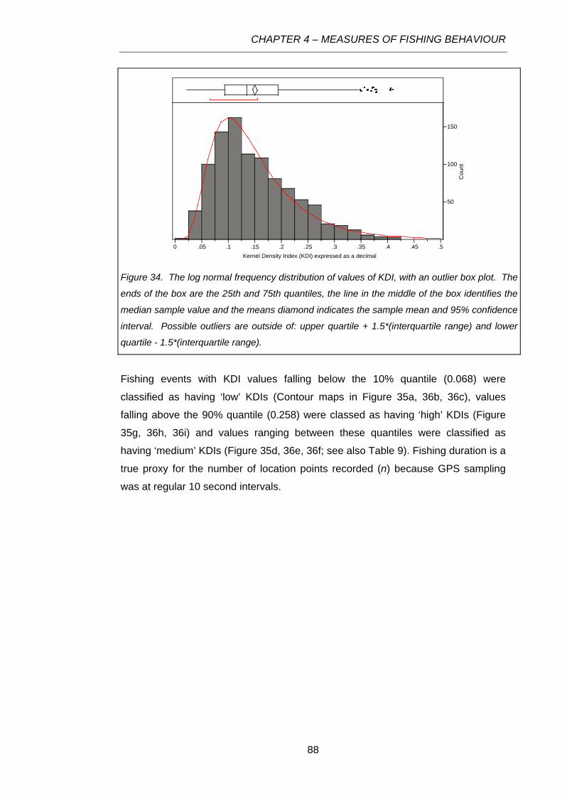
CHAPTER 4 – MEASURES OF FISHING BEHAVIOUR
Fishing events with KDI values falling below the 10% quantile (0.068) were
classified as having ‘low’ KDIs (Contour maps in Figure 35
Figure
35
a, 36b, 36c), values
falling above the 90% quantile (0.258) were classed as having ‘high’ KDIs (
g, 36h, 36i) and values ranging between these quantiles were classified as
having ‘medium’ KDIs (Figure 35d, 36e, 36f; see also Table 9). Fishing duration is a
true proxy for the number of location points recorded (n) because GPS sampling
was at regular 10 second intervals.
50
100
150
Cou
nt
0 .05 .1 .15 .2 .25 .3 .35 .4 .45 .5Kernel Density Index (KDI) expressed as a decimal
Figure 34. The log normal frequency distribution of values of KDI, with an outlier box plot. The
ends of the box are the 25th and 75th quantiles, the line in the middle of the box identifies the
median sample value and the means diamond indicates the sample mean and 95% confidence
interval. Possible outliers are outside of: upper quartile + 1.5*(interquartile range) and lower
quartile - 1.5*(interquartile range).
88

CHAPTER 4 – MEASURES OF FISHING BEHAVIOUR
0 60 12030 Meters 0 90 18045 Meters 0 100 20050 Meters
a b c Probability contour50
95
0 25 5012.5 Meters0 30 6015 Meters0 50 10025 Meters
d e f
0 10 205 Meters 0 20 4010 Meters 0 10 205 Meters
g h i
Figure 35. Contour maps of fishing events with kernel density ratios ranging from very low
(a) to very high (i). Proportion of total dive time is shown as a percentage in the colour
legend. Note different scales of distance. See values of calculated ratios in Table 9.
89

CHAPTER 4 – MEASURES OF FISHING BEHAVIOUR
Dives of longer duration tend to have lower KDIs (Table 9
Table 9. Calculated KDI for the fishing events in
and Figure 36b). Short
fishing events had both small and large KDIs, whereas longer fishing events always
had a small KDIs (when duration >200 min, KDI <0.2). The relationship between
KDI and KDE95 area was also not linear (Figure 36a). ‘Small’ fishing events (those
that covered a small area) had both small and large KDIs while ‘large’ fishing
events had only small KDIs. KDIs quantify the relationship between fishing event
duration or ‘size’ and the degree of heterogeneity of effort distribution during the
event. The longer a fishing event, and the larger the area that was covered during
the event, the less homogenous the distribution of effort during that event.
Figure 35 (a to i): n = the number of
location points recorded. A low KDI (e.g. <0.05) indicates that half of the fishing event was
spent in a small part (e.g. <5%) of the total area covered during the dive, and thus that effort
distribution was heterogeneous.
n KDIfishing duration
(minutes)95% area (metres2) KDI class
50% area (metres2)
a low 690 0.023 115 23996 564
low 852 0.031 142 30433 949b c low 624 0.034 104 17886 614
d medium 252 0.118 42 18874 2220
medium 336 0.118 56 6153 727e f medium 300 0.118 50 5664 669
g high 108 0.302 18 2893 874
high 30 0.336 5 2691 905h i high 144 0.338 24
2671 901
a b Figure 36. Bivariate plots of KDI expressed as a percentage against area of the 95%
contour polygon (a) and fishing duration (b).
90
CHAPTER 4 – MEASURES OF FISHING BEHAVIOUR
Utility of cumulative Kernel Density Index and Duration to identify effort
‘hotspots’ within a fishing event
Analysis of a single fishing event for KDI value with increasing time steps of defined
duration has isolated brief periods of high effort spatial concentration within a
predominantly homogenous search path. This dive is also shown in Figure 36b.
Figures 36a and c also show long distance dives with small areas of slow
movement. In the example in Figure 37 fishing effort was concentrated to the
beginning of the fishing event, with 50 percent of event duration spent in 3 percent
of the total area at the conclusion of the dive (KDI of 0.031 at 142 minutes). The 50
percent density contour was completely contained within the first hour of the 140+
minute dive (Figure 37f, c.f. Figure 37i). The low KDI of the dive reflects the high
vessel speed for part of the dive. See Appendix 3 for data tables and all contours in
10 minute increments.
The slope of the line segments between successive KDIs is related to the rate of
search area increase (Figure 38). A peak in the plot indicates that the vessel
stopped moving or spent a lot of time in a small area, and a continual decline in KDI
with duration indicates that during that period a vessel covered a steadily growing
area.
91
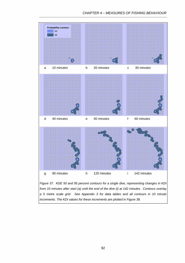
CHAPTER 4 – MEASURES OF FISHING BEHAVIOUR
a 10 minutes c 30 minutesb 20 minutes
Probability contour50
95
d 40 minutes f 60 minutese 50 minutes
g 90 minutes i 142 minutesh 120 minutes
Figure 37. KDE 50 and 95 percent contours for a single dive, representing changes in KDI
from 10 minutes after start (a) until the end of the dive (i) at 142 minutes. Contours overlay
a 5 metre scale grid. See Appendix 3 for data tables and all contours in 10 minute
increments. The KDI values for these increments are plotted in Figure 38.
92
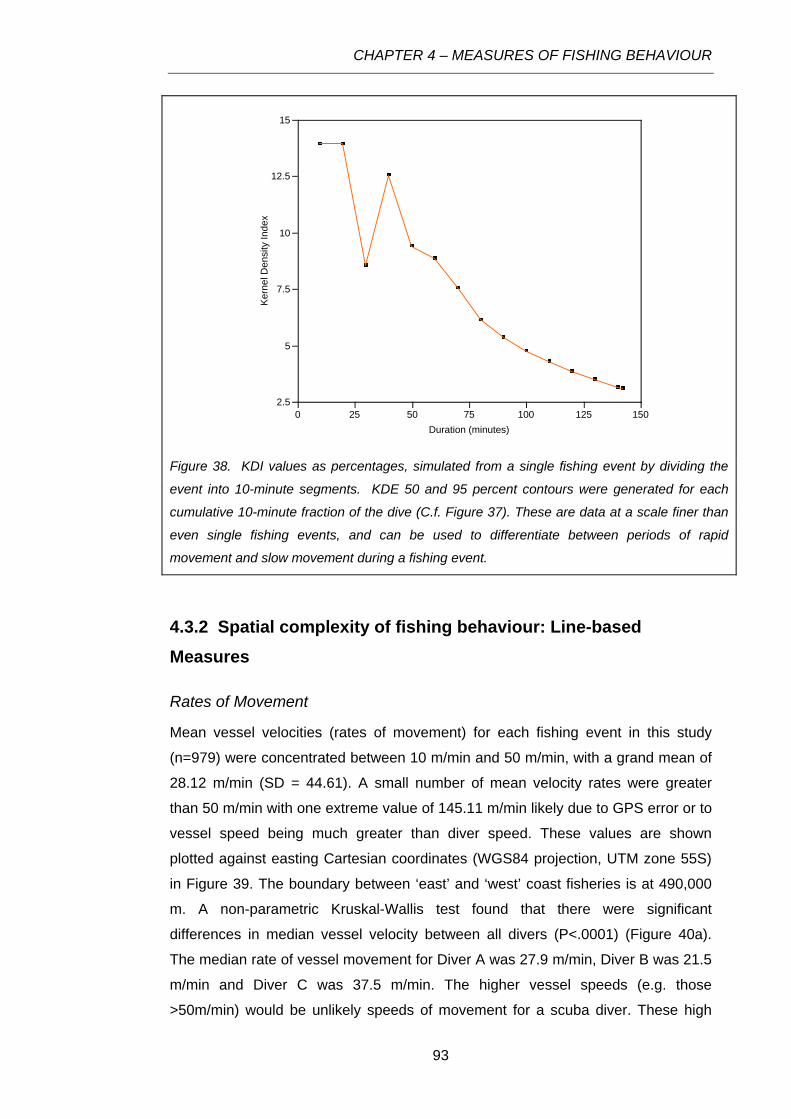
CHAPTER 4 – MEASURES OF FISHING BEHAVIOUR
4.3.2 Spatial complexity of fishing behaviour: Line-based Measures
Rates of Movement
Mean vessel velocities (rates of movement) for each fishing event in this study
(n=979) were concentrated between 10 m/min and 50 m/min, with a grand mean of
28.12 m/min (SD = 44.61). A small number of mean velocity rates were greater
than 50 m/min with one extreme value of 145.11 m/min likely due to GPS error or to
vessel speed being much greater than diver speed. These values are shown
plotted against easting Cartesian coordinates (WGS84 projection, UTM zone 55S)
in Figure 39. The boundary between ‘east’ and ‘west’ coast fisheries is at 490,000
m. A non-parametric Kruskal-Wallis test found that there were significant
differences in median vessel velocity between all divers (P<.0001) (Figure 40a).
The median rate of vessel movement for Diver A was 27.9 m/min, Diver B was 21.5
m/min and Diver C was 37.5 m/min. The higher vessel speeds (e.g. those
>50m/min) would be unlikely speeds of movement for a scuba diver. These high
2.5
5
7.5
10
12.5
15
Ker
nel D
ensi
ty In
dex
0 25 50 75 100 125 150Duration (minutes)
Figure 38. KDI values as percentages, simulated from a single fishing event by dividing the
event into 10-minute segments. KDE 50 and 95 percent contours were generated for each
cumulative 10-minute fraction of the dive (C.f. Figure 37). These are data at a scale finer than
even single fishing events, and can be used to differentiate between periods of rapid
movement and slow movement during a fishing event.
93

CHAPTER 4 – MEASURES OF FISHING BEHAVIOUR
speeds suggest that vessel speed is not a reliable proxy for diver speed. There
were also significant differences in median vessel velocity between aggregated
east and aggregated west coast data (P=.0025) (Figure 40b). The differences
between east and west coast velocities were small, with a median rate of
movement on east coast of 27.3 m/min and west coast of 28.9 m/min. The small
degree of difference between east and west coasts makes it unlikely to be
meaningful despite being statistically significant.
020406080
100120140
Mea
n ve
loci
ty(m
/min
)
250000 300000 350000 400000 450000 500000 550000 600000 650000Ecentroid
Figure 39. Mean vessel velocity for each fishing event in this study (n=979), plotted against
WGS84 UTM 55S Eastings. The boundary between ‘east’ and ‘west’ coast fisheries is at
490,000 m. A horizontal red line demarcates the mean value 28.12 (SD = 44.61). A frequency
distribution plot on the right y-axis shows velocity outliers above 50m/min.
0
102030
5060708090
100110
130140150
Mea
n ve
loci
ty(m
/min
)
Diver A Diver B Diver C
0102030405060708090
100110120130140150
Mea
n ve
loci
ty(m
/min
)
E W Figure 40. Median vessel velocity for each fishing event grouped by Diver (a) and by coast (b). A
non-parametric Kruskal-Wallis test found that there are significant differences in median vessel
velocity between all divers (A: n=228, B: n=436, C: n=320) and between aggregated east and
aggregated west coast data (E: n=439, W: n=540).
bba a
94
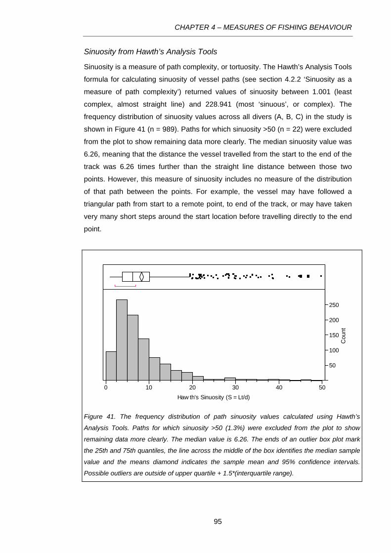
CHAPTER 4 – MEASURES OF FISHING BEHAVIOUR
Sinuosity from Hawth’s Analysis Tools
Sinuosity is a measure of path complexity, or tortuosity. The Hawth’s Analysis Tools
formula for calculating sinuosity of vessel paths (see section 4.2.2 ‘Sinuosity as a
measure of path complexity’) returned values of sinuosity between 1.001 (least
complex, almost straight line) and 228.941 (most ‘sinuous’, or complex). The
frequency distribution of sinuosity values across all divers (A, B, C) in the study is
shown in Figure 41 (n = 989). Paths for which sinuosity >50 (n = 22) were excluded
from the plot to show remaining data more clearly. The median sinuosity value was
6.26, meaning that the distance the vessel travelled from the start to the end of the
track was 6.26 times further than the straight line distance between those two
points. However, this measure of sinuosity includes no measure of the distribution
of that path between the points. For example, the vessel may have followed a
triangular path from start to a remote point, to end of the track, or may have taken
very many short steps around the start location before travelling directly to the end
point.
50
100
150
200
250
Cou
nt
0 10 20 30 40 50Haw th's Sinuosity (S = Lt/d)
Figure 41. The frequency distribution of path sinuosity values calculated using Hawth’s
Analysis Tools. Paths for which sinuosity >50 (1.3%) were excluded from the plot to show
remaining data more clearly. The median value is 6.26. The ends of an outlier box plot mark
the 25th and 75th quantiles, the line across the middle of the box identifies the median sample
value and the means diamond indicates the sample mean and 95% confidence intervals.
Possible outliers are outside of upper quartile + 1.5*(interquartile range).
95

CHAPTER 4 – MEASURES OF FISHING BEHAVIOUR
4.3.3 Behavioural indices: quantitative summaries of behaviour for whole fishing events
Dive Duration
There is a distinct break in the frequency distribution of the duration of fishing
events at the 20-25 minute bin, which had approximately 50% of the number of
fishing events of either of the adjacent bins (15-20 or 25-30) (Figure 42). Across all
divers, 21% of fishing events had a duration of <25 minutes (211 events, n=982).
The same pattern of separation between dives shorter than 25 minutes and longer
than 25 minutes was observed when frequency distributions of dive duration were
separated by diver, and by east/west coast (See Appendix 2 for frequency
distributions for each of these classes). The majority of fishing events were
between 25 and 100mins, with 65% of fishing events falling in this band.
Dive depth
The mean diver depth in metres for each fishing event was plotted against GPS
derived eastings (geographic Cartesian coordinates, WGS84 UTM zone 55S) for
the west (n = 550) and east (n = 439) coasts separately (Figure 43 and Figure 44).
Mean and maximum depths on each coast of Tasmania were very similar but depth
20
40
60
Cou
nt
0 10 20 30 40 50 60 70 80 90 100 120 140 160 180 200 220 240 260 280Duration (minutes)
Figure 42. Frequency distribution of the duration of fishing events across all divers and the
entire fishery. In the 15-20 minute bin there were 58 events, in the 20-25 minute bin only
29, and in the 25-30 minute bin 61 fishing events. There is a break in dive duration at 20-
25 minutes (red bar in the histogram).
96
CHAPTER 4 – MEASURES OF FISHING BEHAVIOUR
97
frequency distributions (Figure 45) were different on each coast: on the west coast
distribution was log-normal (Kolmogorov-Smirnov-Lilliefors D=0.040, P=0.037), on
the east coast distribution was normal (Shapiro-Wilk W=0.991, P=0.007). Although
the median dive depth was less on the west coast (5.6 m) than the east coast (6.1
m), there were relatively more deep fishing events (> 12m) on the west coast
(4.9%) than on the east coast (1.3%).
Two-dimensional surfaces of effort distribution by depth and eastings show that on
the west coast, there was a similar range of depths across all eastings (Figure 43
Figure 43
),
whereas on the east coast, the depth range contracted from west to east (Figure
44
Figure 44
). The high density band of shallow fishing events evident in is
associated with the Port Davey region, where there are numerous protected and
shallow reef areas utilised by the fishers. The 80% quantile on the west coast is
contained entirely between easting coordinates 370,000 and 430,000 and 3 and 9
metres depth. On the east coast, the 80% quantile (orange line in )
covers two areas:1) between 490,000 and 520,000 easting and 2 and 10 metres
depth, and 2) between 570,000 and 590,000 easting and 4 and 8 metres depth.
Fishing events located around King Island are included in the figure for the west
coast (Figure 44), with eastings around 235,400. Only three dives were recorded at
King Island, with mean depths of 4.3, 7.5 and 10.6 metres.

0
2
4
6
8
10
12
14
16m
eand
epth
230000 250000 270000 290000 310000 330000 350000 370000 390000 410000 430000 450000 470000 490000EcentroidEasting (WGS84 Zone55S)
Mea
n D
epth
(Met
res)
Figure 43. West Coast: Diver depth for each fishing event plotted against WGS84 UTM zone 55S centroid easting (on the x-axis). N=550, Maximum mean
depth=14.8m, Mean=6.3m. Frequency distribution of easting is on the top horizontal axis and depth on the right vertical axis. The coloured lines represent
quantile density contours at 5% increments.
0
2
4
6
8
10
12
14
16
mea
ndep
th
490000 510000 530000 550000 570000 590000 610000Ecentroid
Easting (WGS84 Zone55S)
Mea
n D
epth
(Met
res)
Figure 44. East Coast: Diver depth for each fishing event plotted against WGS84 UTM zone 55S centroid easting (on the x-axis). N=439, Maximum mean
depth=14.8m, Mean=6.2m. Frequency distribution of easting is on the top horizontal axis and depth on the vertical axis. Density contours are at 5%
increments.
CHAPTER 4 – MEASURES OF FISHING BEHAVIOUR
98

CHAPTER 4 – MEASURES OF FISHING BEHAVIOUR
4.4 Discussion
4.4.1 Spatial complexity of effort distribution
Kernel Density Index as a measure of effort homogeneity
The concept of a Kernel Density Index was conceived during this study as a
potential metric to classify the spatial distribution of fishing effort within a fishing
event. To the best of my knowledge, a relationship between the amount of area
contained within a high density contour and the area contained within a lower
density contour has not been investigated before and using this technique to
quantify point distribution patterns is new. As a result, understanding of the KDI
ratio and how it can be applied has evolved during the study. Initially KDI was
discussed as a measure of effort concentration rather than of effort homogeneity,
however, a measure of concentration implies a quantity (absolute or relative) and
homogeneity implies a pattern, unquantified. For this reason, KDI will be discussed
here as measure of the homogeneity of effort spatial distribution.
1.12.1
6.8
9.1
14.1
16.2 16.2
11.8
8.07.1
4.6
1.60.9
0.2 0.2
25
50
75
Cou
nt
0 1 2 3 4 5 6 7 8 9 10 11 12 13 14 15Mean Depth (Metres)
0.0
2.5
6.9
15.1
13.3
16.4
10.4
12.0
7.8
6.2
2.71.6
2.5
1.1 1.3
25
50
75
100
Cou
nt
0 1 2 3 4 5 6 7 8 9 10 11 12 13 14 15Mean Depth (Metres)
a b
Figure 45. Frequency distribution of mean dive depth (for a fishing event) on the west (a)
and east (b) coasts. Distribution on the west coast is log-normal (N= 550, Mu=1.72,
Sigma=0.50, KSL Goodness of Fit D=0.040285, P=0.0373) and distribution on the east
coast is normal (N=439, mu=6.20, Sigma=2.46, Shapiro-Wilk Goodness of Fit W=0.990693,
P=0.0072). Percentage frequency is reported at the top of each histogram bin.
Fishing behaviour is shaped by the environmental conditions encountered while
fishing. If the weather is calm, the deckhand can idle behind or near the diver. If
there is swell, the deckhand might keep the vessel offshore a small distance to
avoid breaking waves. Wind conditions can influence deckhand behaviour and thus
vessel path. In windy conditions deckhands typically drive upwind of the diver and
99

CHAPTER 4 – MEASURES OF FISHING BEHAVIOUR
float back down with the breeze before moving upwind again, creating a zig-zagged
overlapping vessel path (Mundy 2007). The degree of homogeneity of fishing effort
will be a function of the conditions encountered by the diver and deckhand during a
fishing event, and, the spatial distribution or concentration of abalone on the reef
being fished. A single quantitative value that describes homogeneity of fishing effort
provides a valuable performance measure of the fishery among years. The KDI is
also likely to provide a useful tool to classify different fishing regions or, as a
variable to standardise CPUE data across divers. A further study to specifically test
the KDI index as a classification variable is required. With standardisation, relative
homogeneity as a function of time has additional potential to be used as a measure
of absolute concentration of fishing effort.
The kernel density analysis and subsequent calculation of KDIs for fishing events is
able to distinguish between a more homogenous fishing pattern and a less
homogenous pattern. For a single fishing event, a low KDI means that the spatial
distribution of fishing effort was heterogeneous across the spatial extent of the
event. For a successful fishing event, this might indicate that there are patches of
densely aggregated abalone present, or that the habitat is heterogeneous.
KDI’s from very short duration fishing events cannot be directly compared with
KDI’s from very long duration fishing events. Very short fishing events have by their
nature an homogenous and concentrated distribution of effort because there has
been no time for vessel movement from the original location of diver entry. Across a
number of events and without standardisation for duration, relative duration will
confound comparison of measures of homogeneity. Despite this, in one location
and for fishing events of the same duration, changes in KDI over time will indicate
changes in fishing behaviour, which in turn may either be a result of changing
abalone abundance, or may cause changes to abalone abundance. This is a limited
application of the index.
A very rough standardisation might be applied to the KDI by eliminating fishing
events with short duration prior to comparison of KDIs. The class of ‘non-
successful’ fishing events identified in section 4.3.1 has durations of less than 25
minutes. The KDIs of these short events are not expected to reflect spatial
distribution of available abalone since they are likely to represent instances when
diver entered the water, found few or no abalone and exited again. Imposing a
100
CHAPTER 4 – MEASURES OF FISHING BEHAVIOUR
minimum duration constraint on a dataset will exclude dives considered to be ‘too
short’ to be fishing events.
Kernel Density Index to describe search behaviour during a fishing event
KDI is a more interesting measure when applied, not as a single value to an entire
fishing event, but as a tool to investigate the scale of change of search behaviours
and of search rate. Changes in KDI with time for a single event (section 4.3.1)
describe the distribution of points along the vessel path. For the event investigated
here, most effort was at the beginning of the path and those areas of high
concentration remained even at full path KDI. Changes in KDI in the course of a
dive may indicate the patchiness of abalone where mean KDI will not. This may be
confounded by changes in vessel speed due to environmental factors described in
the second paragraph of section 4.4.1.
The slopes of lines connecting consecutive values of KDI (at regular time steps)
describe the rate of search area increase. Effort ‘hotspots’ were identified as peaks
in a plot of changing KDI with time, indicating that the vessel stopped moving or
spent a lot of time in a small area. A continual decline in KDI with duration indicates
that the vessel was covering a steadily growing amount of area. A count of ‘peaks’
is a count of places where the vessel paused and imposed concentrated effort on
the reef. For this to be useful as a fishery assessment tool the calculation of
cumulative KDI would need to be automated. However, plotting cumulative KDI
against time would mean that a small change in KDI at the start of a dive would
have a greater effect than a large chage in KDI at the end of a dive. .Changes in
KDI along segments of a path would be a better descriptor of changing fishing
patterns during a fishing event.
In bad weather a vessel will sit in a sheltered area while the diver works away from
the boat and then will move to another sheltered area. These ‘hotspots’ in vessel
location do not mean that there are corresponding ‘hotspots’ in diver location.
There is a possibility that this analysis is attempting to quantify diver behaviour at a
finer scale than the information collected for this study. It would be valuable to test
for a relationship between the frequency of KDI peaks and weather conditions.
When weather is bad (i.e. windy, high swell conditions) there may be more KDI
peaks.
101

CHAPTER 4 – MEASURES OF FISHING BEHAVIOUR
KDI values were derived from Kernel Density Estimates generated using the Animal
Movement Analysis ArcView Extension (Hooge 1998) as described in section 3.2.4.
While this is a straightforward procedure, it doesn’t allow batch processing of paths
and is very time consuming. Automation of the process would be necessary in
order to compare large numbers of diver paths. It is worth investing further work to
develop a streamlined process or even partial or complete automation of Kernel
Density analyses and calculation of changes in KDI with time. This would allow
these ratios to become a useful performance measure to identify portions of a dive
with high effort concentration.
4.4.2 Spatial complexity of fishing behaviour: Line-based Measures
Rates of Movement
Median rates of vessel movement during fishing events were significantly different
between the three divers in this study (Figure 41). The three divers fished in
different locations around Tasmania and may have adapted vessel movement to
the environmental conditions encountered at fishing sites. However, it is equally
likely that abalone were distributed different in these locations or that divers differed
in swimming speed due to factors intrinsic to the individuals involved. Rate of
movement is not a very informative line-based measure of the spatial complexity of
fishing behaviour.
Path sinuosity and Fractal Dimension
It has been demonstrated that the scale of forager movement can be relative to the
scale of prey distribution (Marell et al. 2002; Ramos-Fernandez et al. 2004; Austin
et al. 2004; Bertrand et al. 2005). However, there is debate about whether some
more complex movement analyses, including Lévy flights and the fractal dimension
of paths, have been performed and interpreted correctly in this context (Halley et al.
2004; Benhamou 2004; 2007).
As described in section 4.2.2, efforts to describe searching behaviour during this
study using measures of sinuosity and fractal dimension were discontinued
primarily because vessel movement masks the fine-scale movement of divers and
searching patterns cannot be assumed to be visible in the vessel track. However, a
potential application of these line-based techniques is in free dive fisheries such as
102
CHAPTER 4 – MEASURES OF FISHING BEHAVIOUR
the New Zealand Paua (abalone) fishery. Paua divers do not use surface air
supplied or SCUBA and are required to breath-hold while fishing, meaning that they
regularly surface for air during a fishing event. The fishing event then is a
contiguous series of collecting and searching events. Some New Zealand divers
have been bearing GPS loggers on their person while fishing to record diver
position independently of vessel position (Cooper 2006). As the data series
develops, step length distributions could be used to investigate diver foraging
behaviour in that fishery.
4.4.3 Behavioural indices
Dive duration as an indicator of fishing success
The frequency distribution of fishing event duration collected with electronic depth
data loggers permits identification and classification of short duration fishing events
(<25 min). This is not possible with standard fishery reporting systems where effort
(time) is estimated by a diver for the entire day. These short duration dives may be
exploratory, may indicate an absence of commercial quantities of abalone, or on
rare occasions relate to equipment failure. In some cases there may be no abalone
present, or the area may have been fished recently by other divers. Mapping the
spatial distribution of short duration (‘unsuccessful’) fishing events across the
Tasmanian fishery may help to identify locations where divers expect good fishing
conditions, but against expectations do not meet with fishing success. It is unlikely
that short duration dives are related to poor weather conditions (e.g. swell rolling
into a bay), as most commercial divers have sufficient experience to assess
suitability of conditions prior to diving. Repeated short dives at the same location by
different divers and on different days should be seen as a warning that fishing
success has declined at that location. Mapping of these short duration dives over
the entire fleet therefore provides an important indicator of an onset of serial
depletion.
The theory of Ideal Free Distribution proposes that the behaviour of fishers in
distributing effort across a fishery can be used as an index for the abundance of
fish stocks (Branch et al. 2006). Prince & Hilborn (1998) proposed that IFD occurs
in the Tasmanian abalone fishery. In a simple form, effort distribution can be
measured as the number of fishing events or number of hours spent fishing at a
site. Building on the logic behind IFD, a combination of dive frequency and dive
103

CHAPTER 4 – MEASURES OF FISHING BEHAVIOUR
duration might be used to characterise events as ‘successful’ (>25 min duration) or
‘unsuccessful’ (<25 min duration). The potential of dive duration as an indicator of
dive success could be tested by plotting catch against dive duration in future work.
Four scenarios of diver behaviour through time under different regimes of stock
abundance are illustrated in Figure 46
Figure 46
Figure 46
Figure 46
. In an area with healthy stocks there would
be many ‘successful’ and few ‘unsuccessful’ fishing events ( a). When few
or no abalone are present at a site there would be no successful fishing events, and
only a low number of unsuccessful ‘exploratory’ events ( b). An
hypothetical permanent local stock depletion scenario is illustrated in d. It
is hypothesised that as divers learn of local (site) depletion, expressed as several
short ‘unsuccessful’ dives, they will stop returning to fish at that site except perhaps
for occasional short ‘exploratory’ dives to check whether the site has recovered
enough to be profitably fished. If a site were permanently depleted, divers might
eventually stop visiting altogether.
104
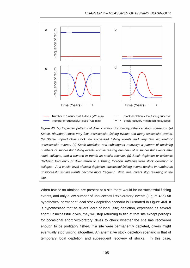
CHAPTER 4 – MEASURES OF FISHING BEHAVIOUR
Stock depletion = low fishing successNumber of ‘unsuccessful’ dives (<25 min)
Number of ‘successful’ dives (>25 min)
Time (Years)
Freq
uenc
y of
retu
rn
Stock recovery = high fishing success
Freq
uenc
y of
retu
rn
Time (Years)
a
dc
b
Figure 46. (a) Expected patterns of diver visitation for four hypothetical stock scenarios. (a)
Stable, abundant stock: very few unsuccessful fishing events and many successful events.
(b) Stable unproductive stock: no successful fishing events and very few ‘exploratory’
unsuccessful events. (c) Stock depletion and subsequent recovery: a pattern of declining
numbers of successful fishing events and increasing numbers of unsuccessful events after
stock collapse, and a reverse in trends as stocks recover. (d) Stock depletion or collapse:
declining frequency of diver return to a fishing location suffering from stock depletion or
collapse. At a crucial level of stock depletion, successful fishing events decline in number as
unsuccessful fishing events become more frequent. With time, divers stop returning to the
site.
When few or no abalone are present at a site there would be no successful fishing
events, and only a low number of unsuccessful ‘exploratory’ events (Figure 46
Figure 46
b) An
hypothetical permanent local stock depletion scenario is illustrated in d. It
is hypothesised that as divers learn of local (site) depletion, expressed as several
short ‘unsuccessful’ dives, they will stop returning to fish at that site except perhaps
for occasional short ‘exploratory’ dives to check whether the site has recovered
enough to be profitably fished. If a site were permanently depleted, divers might
eventually stop visiting altogether. An alternative stock depletion scenario is that of
temporary local depletion and subsequent recovery of stocks. In this case,
105

CHAPTER 4 – MEASURES OF FISHING BEHAVIOUR
following stock recovery the number of long dives would increase as the number of
short dives decreased (Figure 46c). These behavioural scenarios are potential
fishery performance measures, and can be quantified by mapping and monitoring
two aspects of fishing behaviour in tandem: dive duration and dive frequency, over
multiple years.
Differences in diver depth across the fishery
Stock assessments based upon diver estimates of fishing depth have suggested
that divers fish in deeper water on the west coast than on the east and in particular
that a small number of divers fish at depths >20 m at King Island, in the far north
west of the State (Tarbath et al. 2007). Depth as a measure of fishing behaviour
has positively identified different depth patterns on the east and west coasts of
Tasmania, however, in this study more deep dives were recorded on the east coast
than on the west. It was not possible to confirm with depth logger data that deep
diving is occurring off King Island as the sample size of dives at that location was
very small (n=3). Of the 3 dives, one deep dive with mean depth of 10.6 m was
recorded. Other divers not included in this analysis may be participating in deep
diving both off King Island and on the west coast of Tasmania.
The Tasmanian abalone industry divers have a voluntary Code of Practice limiting
the duration and depth to which they dive. For safety reasons, divers must dive to
internationally recognised decompression tables or using a dive computer as
described in the Code (Tasmanian Abalone Council Ltd 2002). To comply with the
dive tables, any deep dive would necessarily be very short. Summaries of dive
depth and dive duration from this study indicate that the divers who participated are
complying with the tables.
Divers may fish deep water when shallow-water abalone stocks are becoming
depleted. This is a simple interpretation of a complex relationship and potentially
confounding factors can be identified. Under conditions of low swell height, divers
are able to fish in shallow water without discomfort or danger. In addition,
irrespective of weather conditions some divers prefer to fish in shallow water while
others prefer to fish in deeper water. The west coast of Tasmania experiences
more bad weather than the east, and divers may rarely fish in shallow water there
because it is too exposed (Mundy 2007). However, changes over time in mean
fishing depth upon a reef might indicate that easily accessible abalone, in shallow
106

CHAPTER 4 – MEASURES OF FISHING BEHAVIOUR
water, have been removed from the population and that divers are moving deeper
to find animals.
4.4.4 Future directions for research
This study has identified a number of useful measures that describe behaviour
during a fishing event. A multivariate approach to assessment that integrates
monitoring of short-duration dive frequency, KDI, depth, duration and area fished
would be much richer than the present CPUE based assessment techniques.
However, understanding the causes and effects of behavioural change on the
performance measures described here and interpreting each measure correctly is a
challenge to applying the measures in a management framework.
There is a complex web of relationships at three spatial scales and across multiple
temporal scales:
• Within event / measures and patterns within a reef
• Whole event / measures specific to a reef/location
• Across events / fishery wide patterns
The analyses described in this chapter address the data at the first two of these
three scales, at the scale of individual vessel movement within single fishing events
(searching behaviours) and descriptive measures that apply to a whole individual
fishing event (behavioural indices). Attempting to derive information about individual
diver behaviour and very subtle changes in the complexity of diver behaviour is
overly optimistic when data collected refer to the movement of a vessel and not the
movement pattern of a diver. In this study, no attempt was made to verify the data
by questioning divers. Any future work would benefit from a formal diver survey to
provide this information. Specifically, recording actual divers’ position (rather than
vessel position) would constitute a significant improvement.
While the analysis must begin with individual fishing events, this allows inferences
only about individual diver behaviour at specific sites and under specific fishing
conditions. When many fishing events are synthesised it may be possible to draw
conclusions about an area rather than about the divers that visit that area, providing
that results are standardised by diver. Due to the limitations of a small dataset it
has not been possible to realistically investigate fleet dynamics or effort distribution
107

CHAPTER 4 – MEASURES OF FISHING BEHAVIOUR
108
for the Tasmanian abalone fishery. In the current absence of sufficient data, I have
worked on “proof of concept” only.
There is much potential for investigation into the broader scale application of
distribution of fishing effort around the coast, which does not depend on the
dynamics of an individual fishing event. A study of spatial effort distribution based
upon information about vessel position will be more robust at a spatial scale greater
than individual fishing trips so that distinguishing between vessel and diver
movements is irrelevant.

CHAPTER 5 – CONCLUSIONS
CHAPTER 5 CONCLUSIONS
5.1 Conclusions of the study
Traditional fishery stock assessment methods that are reliant on coarse scale
fishery-dependent reports of catch and effort have failed to predict or detect the
depletion or collapse of many abalone fisheries around the world. This study
provides a first step towards applying spatial analysis techniques to very fine scale
spatial data so as to better capture the risk of serial depletion in abalone fisheries.
For the first time in a commercial abalone fishery, the fishing distribution and effort
data analysed for this project were collected by fishers at the scale of individual
fishing events. Fishing location and duration data were not spatially aggregated
and localised heterogeneity of fishing effort distribution was not ‘masked’ in fishing
effort indices, which is common in traditional fishery data collection practices.
The spatial data provided by GPS and depth loggers are amenable to three types
of analyses:
• Analyses based on traditional Catch Rate performance indices
• Analyses that account for the estimated area searched by a diver and on
search behaviour patterns of a diver within a single fishing event
• Analyses at a larger scale incorporating the spatial and temporal dynamics
of fishing location
This study demonstrated techniques for calculating catch rate performance indices
from fine scale spatial data and assessed some potential quantitative methods for
describing the search behaviour patterns of divers. Broad-scale adoption across
the Tasmanian abalone fishery of GPS and depth data collection tools would open
the way for higher level analyses and monitoring of spatial and temporal patterns in
fishing activity. There is great promise for improved management of the abalone
fishery in the application of some of the techniques explored in this study, provided
that sufficient good quality spatial data can be collected with the assistance of
abalone divers working in the Tasmanian abalone fishery.
5.1.1 Tools for fishery assessment
This study demonstrated that reporting of dive time by divers introduces a highly
variable error in fishing time estimate. However, errors in time reporting did not
significantly affect CPUE values here. These results would benefit from further
investigation across a larger sample. When the instruments are functioning
109
CHAPTER 5 – CONCLUSIONS
correctly, depth logger records of dive duration can provide an accurate measure of
the amount of time a diver has spent fishing and improve the accuracy of CPUE
measures. The use of electronic depth data loggers provides detailed information
on dive times and is a major advance to current fishery reporting systems, where
effort (time) is estimated by a diver for the entire day. The loggers also allow
detection of the frequency of short dives (< 25 min) that may indicate an absence of
commercial quantities/densities of abalone. An increase in the ratio of short to long
dives over time, combined with an increase in the number of dives per day, may
indicate depletion of a stock.
The collection of spatial coordinates every 10 secs allows both linear (path) and two
dimensional (area) parameters to be calculated for each fishing event. The length
of path laid down by a vessel, distance (D), is an imperfect measure of diver effort
because a) the relationship between vessel movement and diver activity is
unknown, and b) distance along a line is a single-dimensional measure only and
alone doesn’t indicate the spatial concentration of effort distribution. Until the
position of a diver relative to the fishing vessel can be quantified, it is essential to
keep in mind that the distance (D) the vessel travelled during a fishing event may
be a reflection of the skipper behaviour and weather conditions at the time rather
than a reflection of diver’s position on the reef. Of three techniques used to
estimate the fishing area available to a diver during a fishing event, different Catch
per Unit of Area (CPUA) metrics were derived. However, the value and precision of
these metrics could be further explored. Further fieldwork, involving the close
monitoring of divers, is necessary to determine how closely area and effort
distribution estimates reflect the actual amount of area searched by a diver during a
fishing event.
Overall, results suggest that these novel spatial indices of CPUE can be used in
combination with time-based CPUE to characterise the differences in individual
divers’ foraging behaviour. These new indices could be useful to characterise
different types of fishing behaviour between individual divers across the Tasmanian
abalone fishery. All indices of catch-rates (time-based, distance-based, area-
based) analysed in this study revealed discrepancies in individual fishers’
behaviour. With the example of a small sample from the Tasmanian abalone
fishery, this study does demonstrate the value of fine-scale monitoring of fishing
effort for the management of small-scale coastal fisheries. This preliminary study
110

CHAPTER 5 – CONCLUSIONS
suggests a potential to better account for differences in individual fishers’
harvesting behaviour in fishery management and assessment.
Kernel density estimates were analysed in a novel way to generate a Kernel
Density Index for classifying homogeneity in fishing effort distribution for each
fishing event. Variation in KDI can be used to provide information on homogeneity
of foraging activity during a fishing trip. With the appropriate time resolution to
monitor divers’ position, KDI over a whole dive may provide information on density,
with the limitation that other factors may also influence vessel movement. Line-
based statistics also provide information about the spatial homogeneity of effort
distribution, however, these descriptors resolve movement from the track of a
fishing vessel only and they cannot be used to understand diver movement
underwater.
5.1.2 Lessons learnt
Considerable problems with the design of early models of GPS loggers resulted in
patchy loss of data, and meant that some data were missing from many days of
data collection. The marine environment presents challenges in electronics design.
Electronic equipment that is to be used in fishing boats must be designed with
practicality as a top priority. Instruments and loggers must be very robust,
waterproof and ideally would be self-contained and need minimal handling or user
interaction. The SciElex GPS loggers were designed and built for use by abalone
fishers and fishery researchers, with development starting in 2004. Hardware
development and testing is ongoing and the equipment is continually being
improved. However, working with a contracted company to build a customised data-
logging system has taken time, funds, and there is no rigorous testing program in
place. The time and money overhead associated with technology development is
an important factor for others to allow for when considering using data logging
systems for fisheries research. At this time there is still no cost-effective commercial
alternative to the project-designed loggers, however, with a growing commercial
market for personal GPS loggers for geotagging and for personal aviation
enthusiasts, the capability and affordability of commercial products is rapidly
increasing (<US$200.00), and a suitable commercial product may be available
soon.
Diver participation in the research program was voluntary and participation
numbers increased from two divers in 2005, to approximately 20 divers in 2007.
111

CHAPTER 5 – CONCLUSIONS
This represented twenty percent of the active divers working in the fishery. In 2009,
61 divers were participating in the data collection program. Divers who have
participated in the program were generally engaged and careful when using the
data loggers, however, catching abalone is necessarily their first priority. Divers,
and volunteers in general may not pay the same attention to detail as a researcher
who can focus solely on obtaining high quality data. The issues associated with
volunteer fishery monitoring and data collection have been broadly discussed in
literature (Barrett et al. 2002, Danielsen et al. 2005) and the value of voluntary
participation in data collection is well recognised (Gerdeaux and Janjua 2009).
However, the system needs to be robust, both in the practicality of protocol and the
hardware design.
5.2 Future directions for research
This study has started to consider different approaches that will quantify the fine
scale spatial distribution of fishing effort in the Tasmanian abalone fishery. Before
many of the indices explored can be applied in a management framework, they
need to be validated through field testing. Before behavioural indices can be used
with confidence, studies must be done to:
a) Evaluate the information loss from apportioning daily catch across multiple
fishing events in a day. Fine scale catch weight reporting (catch per dive)
was not within the scope of this study. Hanging scales might be used to
measure the approximate weight of each bag of abalone caught as it is lifted
from the water, however, accuracy would be compromised by working on a
rolling boat. Deckhand estimates of catch weight per bag might be sufficient
if estimates were regularly calibrated against shore-side measurements.
b) Quantify the relationship between diver movement and vessel movement.
Investigations into fishing behaviour of divers use boat movement as
proxies for effort distribution. To correctly apply the most fine-scaled
movement analyses to single fishing events, it would be idea to know the
precise movement of divers. Alternatively, in the absence of such validation,
interpretation of the data could be limited to scales of 100’s metres rather
than 10’s of metres.
c) Quantify relationships between fishing behaviour and stock status.
Depletion experiments are designed to estimate the catchability of target
species using sampling gear and could be employed to evaluate the new
technology and methods. A depletion experiment could be designed to test
the behaviour of both traditional and new abundance indices when a real
112

CHAPTER 5 – CONCLUSIONS
113
stock depletion takes place. Rago et al. (2006) propose a spatial model that
is suitable for sessile benthic invertebrates that does not depend on
restrictive and prohibitive assumptions.
d) Develop and apply analytical techniques that can categorise different diver
activities within a stream of GPS data. Some data were excluded from this
study due to loss of depth data. Models that distinguish between vessel
activities (e.g. travelling, fishing, and resting) may reduce loss of data due to
failure in the depth logger component.
Knowledge of the spatial location of each fishing event (dive) enables analysis of
individual, and fleet, fishing behaviour. Behavioural phase shift studies that build on
movement step-length analyses have potential as techniques to capture detail of
the activities performed during a fishing event, e.g. shift in behaviours between
foraging and moving between patches.
Spatial performance measures, incorporating indices that have been validated by
fishery independent abalone population surveys, will ensure that spatial serial
depletion does not go undetected in the Tasmanian abalone fishery. Spatial
performance measures could help to address questions that are essential to the
management of abalone resources. Questions of interest that are dependent on
fine-scale spatial data are:
• How often do divers revisit particular locations?
• Does the scale of fishing match the scale of stock distribution?
• Can areas of different productivity be identified through characterising
the fishing behaviour of divers?
• Can changes in fishing patterns/behaviour be detected from year to year
and are they related to the state of the stock?
• Can the time taken for an area to recover from overfishing be monitored
– i.e. how long must an area “rest” before catch rates return to earlier
levels?
Answers to these questions will help to characterise the spatial variation in the
productivity of different abalone populations.

APPENDIX 1
APPENDIX 1: Geoprocessing Inputs and Settings Geoprocessing Box 1. Options for Hawth’s Analysis Tools Version 3.21 for ArcGIS Create
Minimum Convex Polygons
Hawth’s Analysis Tools: Animal Movements: Create Minimum Convex Polygons
Point locations layer Projected vessel position data
Omit “0” location coordinates Yes
Create a different MCP for each unique value in this field Drop Code
Output shapefile Minimum Convex Polygon
Geoprocessing Box 2. Options for Hawth’s Analysis Tools Version 3.21 for ArcGIS Add
Area/Perimeter Fields To Table
Hawth’s Analysis Tools: Table Tools: Add Area/Perimeter Fields To Table (polygons)
Polygon feature layer Buffer polygon
Area Selected
Convert area units No
Perimeter Selected
Convert perimeter units No
Geoprocessing Box 3. Options for ArcInfo 9.2 Buffer Analysis
ArcToolbox: Analysis Tools: Proximity: Buffer
Input features Vessel path (line)
Output features Buffer polygon
Distance 30 metres
Side type Full
End type Round
Dissolve type
None
114

APPENDIX 1
Geoprocessing Box 4. Options for Hawth’s Analysis Tools Version 3.21 for ArcGIS Convert
Locations To Paths
Hawth’s Analysis Tools: Animal Movements: Convert Locations to Paths (points to lines)
Point locations layer Projected vessel position data
Create multiple output paths using ‘drop code’
field to distinguish between different paths Path options
Make each segment a separate line No
Ordering Data to be sorted using date/time field
Output shapefile Vessel path (line)
115
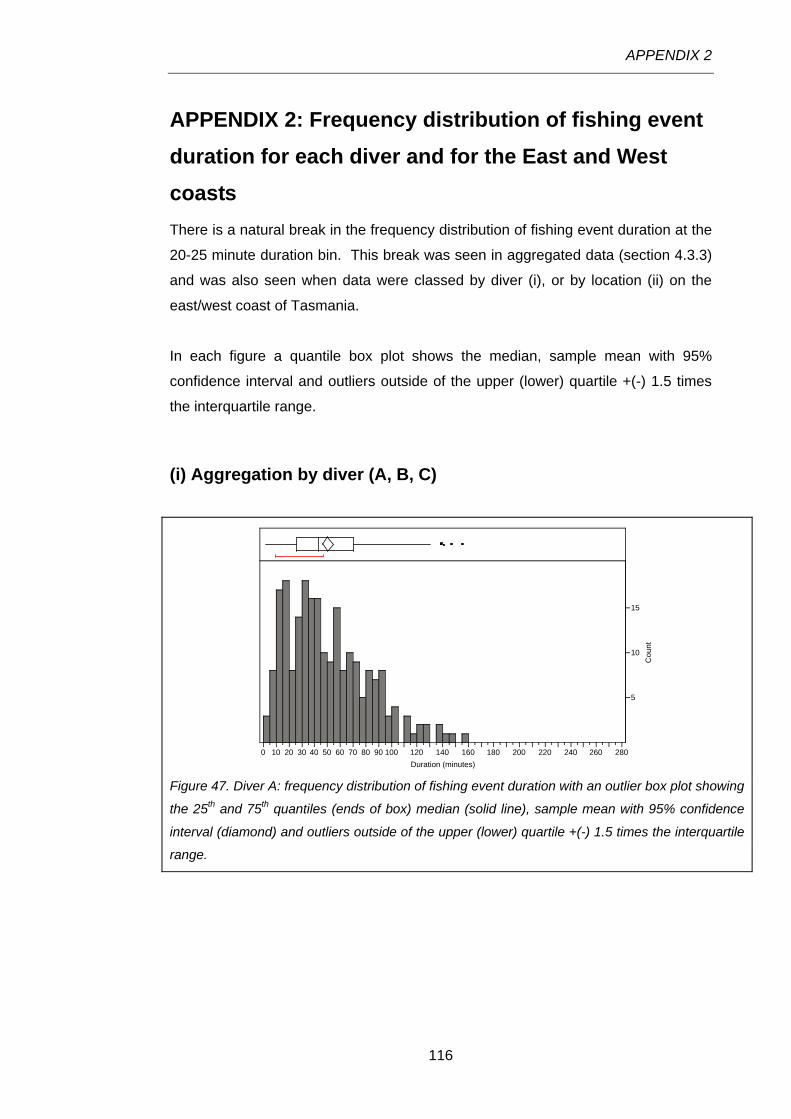
APPENDIX 2
APPENDIX 2: Frequency distribution of fishing event duration for each diver and for the East and West coasts There is a natural break in the frequency distribution of fishing event duration at the
20-25 minute duration bin. This break was seen in aggregated data (section 4.3.3)
and was also seen when data were classed by diver (i), or by location (ii) on the
east/west coast of Tasmania.
In each figure a quantile box plot shows the median, sample mean with 95%
confidence interval and outliers outside of the upper (lower) quartile +(-) 1.5 times
the interquartile range.
(i) Aggregation by diver (A, B, C)
5
10
15
Cou
nt
0 10 20 30 40 50 60 70 80 90 100 120 140 160 180 200 220 240 260 280Duration (minutes)
Figure 47. Diver A: frequency distribution of fishing event duration with an outlier box plot showing
the 25th and 75th quantiles (ends of box) median (solid line), sample mean with 95% confidence
interval (diamond) and outliers outside of the upper (lower) quartile +(-) 1.5 times the interquartile
range.
116

APPENDIX 2
10
20
30
Cou
nt
0 10 20 30 40 50 60 70 80 90 100 120 140 160 180 200 220 240 260 280Duration (minutes)
Figure 48. Diver B: frequency distribution of fishing event duration with an outlier box plot
showing the 25th and 75th quantiles (ends of box) median (solid line), sample mean with 95%
confidence interval (diamond) and outliers outside of the upper (lower) quartile +(-) 1.5 times
the interquartile range.
5
10
15
20
25
Cou
nt
0 10 20 30 40 50 60 70 80 90 100 120 140 160 180 200 220 240 260 280Duration (minutes)
Figure 49. Diver C: frequency distribution of fishing event duration with an outlier box plot
showing the 25th and 75th quantiles (ends of box) median (solid line), sample mean with 95%
confidence interval (diamond) and outliers outside of the upper (lower) quartile +(-) 1.5 times
the interquartile range.
117

APPENDIX 2
(ii) Aggregation by location (east/west coast of Tasmania)
10
20
30
Cou
nt
0 10 20 30 40 50 60 70 80 90 100 120 140 160 180 200 220 240 260 280Duration (minutes)
Figure 50. East coast: frequency distribution of fishing event duration with an outlier box plot
showing the 25th and 75th quantiles (ends of box) median (solid line), sample mean with 95%
confidence interval (diamond) and outliers outside of the upper (lower) quartile +(-) 1.5 times
the interquartile range.
10
20
30
40C
ount
0 10 20 30 40 50 60 70 80 90 100 120 140 160 180 200 220 240 260 280Duration (minutes)
Figure 51. West coast: frequency distribution of fishing event duration with an outlier box plot
showing the 25th and 75th quantiles (ends of box) median (solid line), sample mean with 95%
confidence interval (diamond) and outliers outside of the upper (lower) quartile +(-) 1.5 times
the interquartile range.
118

APPENDIX 3
APPENDIX 3: Changes in Kernel Density Index with increasing fishing event duration – data table and plots
The effects of dive duration on Kernel Density Index (KDI) were simulated using a
single fishing event with a low KDI as a case study (section 4.3.1). The dive
chosen had a full duration of 142 minutes. The dataset of vessel location was
divided into 10 minute sub-samples and KDI evolution simulated in 10 minute
increments, starting with the first 10 minutes of the dive and progressing to the full
duration (a - n).
Table 10. The changing value of KDI as the duration of a fishing event increases.
Contour area (ha)
Duration (mins) 50 percent 95 percent KDI
a 10 0.059 0.421 13.953
b 20 0.059 0.421 13.953
c 30 0.058 0.673 8.546
d 40 0.095 0.758 12.568
e 50 0.082 0.867 9.438
f 60 0.094 1.059 8.871
g 70 0.098 1.301 7.550
h 80 0.093 1.523 6.129
i 90 0.094 1.758 5.352
j 100 0.096 2.016 4.768
k 110 0.097 2.245 4.304
l 120 0.095 2.453 3.864
m 130 0.095 2.712 3.512
n 140 0.095 3.026 3.138
o 142 0.095 3.043 3.120
119

APPENDIX 3
120
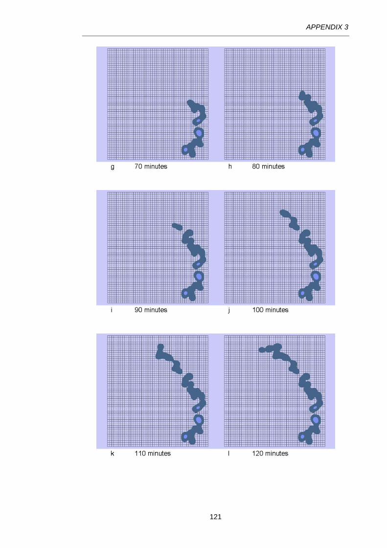
APPENDIX 3
121

APPENDIX 3
122

APPENDIX 4
APPENDIX 4: ANOVA output tables For the main analysis, degrees of freedom (Df), mean square (MS), F-value (F) and
p-value (P) are specified for each effect. Significant p-values are in bold print: (p <
0.05). When a main effect is significant, parameter mean estimates, standard error,
and p-values are given for each level. When one of the main effects is significant
then a detailed table of the post-hoc comparisons for this factor is shown.
Table 11. Results of the 2-way ANOVA testing effects of individual divers (Diver) and time-
based CPUE (Method: CPUEdiver or CPUEdata logger) on the catch-rate estimates.
Df MS F P
Diver 2 12410.8 6.7028 0.0014
Method 1 62.6 0.0338 0.8542
Diver:Method 2 74.2 0.0401 0.9607
Residuals 292 851.6
Diver Diff Lwr Upr P
B-A 31.521 10.141 52.901 0.002 C-A 33.287 11.103 55.471 0.001 C-B 1.766 -10.837 14.369 0.942
Table 12. Results of the 1-way ANOVA testing for significant differences in distance-based
CPUE (CPUD) between individual divers (Diver).
Df MS F P
Diver 2 70466 11.543 2.218e-05
Residuals 146 3052
Diver Diff Lwr Upr P
C-A 10.499 -29.990 50.988 0.813
B-A 51.852 12.831 90.873 0.006 B-C 41.353 18.351 64.355 1.089E-04
123

APPENDIX 4
Table 11. Results of the 2-way ANOVA testing effects of individual divers (Diver) and area-
estimating methods (Method: Abuf, Amcp or Akde) on search area (log-transformed).
Df MS F P
Diver 2 1.68 3.9 0.021
Method 2 9.37 21.6 < 1e-09
Diver*Method 4 0.81 1.9 0.117
Residuals 438 0.43
Method:Diver Diff Lwr Upr P
Akde:B- Amcp:A 0.209 -0.404 0.822 0.979
Akde:A- Amcp:A 0.302 -0.504 1.108 0.963
Akde:C- Amcp:A 0.408 -0.228 1.043 0.546
Abuf:A- Amcp:A 0.443 -0.363 1.249 0.738
Amcp:C- Amcp:A 0.481 -0.155 1.117 0.309
Amcp:B- Amcp:A 0.567 -0.046 1.180 0.095
Abuf:B- Amcp:A 0.809 0.196 1.421 0.002 Abuf C- Amcp:A 0.835 0.199 1.471 0.002 Akde:A- Akde:B 0.093 -0.520 0.706 1.000
Akde:C- Akde:B 0.199 -0.162 0.560 0.737
Abuf:A- Akde:B 0.234 -0.378 0.847 0.958
Amcp:C- Akde:B 0.273 -0.089 0.634 0.313
Amcp:B- Akde:B 0.358 0.039 0.677 0.015 Abuf:B- Akde:B 0.600 0.281 0.919 3E-07 Abuf:C- Akde:B 0.626 0.265 0.987 3.9E-06 Akde:C- Akde:A 0.106 -0.530 0.742 1.000
Abuf:A- Akde:A 0.141 -0.665 0.947 1.000
Amcp:C- Akde:A 0.179 -0.456 0.815 0.994
Amcp:B- Akde:A 0.265 -0.348 0.878 0.916
Abuf:B- Akde:A 0.507 -0.106 1.120 0.199
Abuf:C- Akde:A 0.533 -0.103 1.169 0.184
Abuf:A- Akde:C 0.036 -0.600 0.671 1.000
Amcp:C- Akde:C 0.074 -0.325 0.473 1.000
Amcp:B- Akde:C 0.160 -0.202 0.521 0.906
Abuf:B- Akde:C 0.401 0.040 0.762 0.017 Abuf:C- Akde:C 0.427 0.028 0.826 0.026
124

APPENDIX 4
Amcp:C- Abuf:A 0.038 -0.598 0.674 1.000
Amcp:B- Abuf:A 0.124 -0.489 0.737 0.999
Abuf:B- Abuf:A 0.366 -0.247 0.978 0.642
Abuf:C- Abuf:A 0.392 -0.244 1.027 0.600
Amcp:B- Amcp:C 0.086 -0.275 0.447 0.998
Abuf:B- Amcp:C 0.327 -0.034 0.689 0.111
Abuf:C- Amcp:C 0.353 -0.046 0.752 0.131
Abuf:B- Amcp:B 0.242 -0.077 0.560 0.308
Abuf:C- Amcp:B 0.268 -0.094 0.629 0.339
Abuf:C- Abuf:B 0.026 -0.335 0.387 1.000
Table 13. Results of the 2-way ANOVA testing effects of individual divers (Diver) and area-
based CPUE (Method: CPUAbuf, CPUAmcp or CPUAkde) on the catch-rate estimates. The
results are presented for the log transformed CPUA data.
Response: log(Value) Df Sum Sq Mean Sq F value Pr(>F)
Diver 2 1.484 0.742 1.171 0.311
Method 2 18.456 9.228 14.570 *** 7.48E-07
Diver:Method 4 11.602 2.901 4.580 ** 0.001
Residuals 438 277.412 0.633
Diver:Method Diff Lwr Upr P
C: CPUAbuf -B: CPUAmcp 0.022 -0.415 0.458 1.000
B: CPUAbuf -B: CPUAmcp 0.118 -0.267 0.503 0.989
A: CPUAkde -B: CPUAmcp 0.148 -0.592 0.888 0.999
C: CPUAmcp -B: CPUAmcp 0.272 -0.164 0.708 0.583
A: CPUAbuf -B: CPUAmcp 0.435 -0.305 1.175 0.660
C: CPUAkde -B: CPUAmcp 0.539 0.102 0.975 0.004
B: CPUAkde -B: CPUAmcp 0.652 0.267 1.038 7.200E-06
A: CPUAmcp -B: CPUAmcp 0.815 0.075 1.555 0.019
B: CPUAbuf -C: CPUAbuf 0.097 -0.340 0.533 0.999
A: CPUAkde -C: CPUAbuf 0.127 -0.641 0.895 1.000
C: CPUAmcp -C: CPUAbuf 0.251 -0.231 0.733 0.793
A: CPUAbuf -C: CPUAbuf 0.414 -0.354 1.182 0.759
125

APPENDIX 4
126
C: CPUAkde -C: CPUAbuf 0.517 0.035 0.999 0.025
B: CPUAkde -C: CPUAbuf 0.631 0.195 1.067 2.857E-04
A: CPUAmcp -C: CPUAbuf 0.794 0.026 1.561 0.037
A: CPUAkde -B: CPUAbuf 0.030 -0.710 0.770 1.000
C: CPUAmcp -B: CPUAbuf 0.154 -0.282 0.590 0.974
A: CPUAbuf -B: CPUAbuf 0.317 -0.423 1.057 0.920
C: CPUAkde -B: CPUAbuf 0.420 -0.016 0.857 0.069
B: CPUAkde -B: CPUAbuf 0.534 0.149 0.919 0.001
A: CPUAmcp -B: CPUAbuf 0.697 -0.043 1.437 0.083
C: CPUAmcp -A: CPUAkde 0.124 -0.644 0.892 1.000
A: CPUAbuf -A: CPUAkde 0.287 -0.686 1.260 0.992
C: CPUAkde -A: CPUAkde 0.390 -0.378 1.158 0.813
B: CPUAkde -A: CPUAkde 0.504 -0.236 1.244 0.458
A: CPUAmcp -A: CPUAkde 0.667 -0.306 1.640 0.450
A: CPUAbuf -C: CPUAmcp 0.163 -0.605 0.931 0.999
C: CPUAkde -C: CPUAmcp 0.266 -0.216 0.748 0.732
B: CPUAkde -C: CPUAmcp 0.380 -0.056 0.817 0.145
A: CPUAmcp -C: CPUAmcp 0.543 -0.225 1.311 0.405
C: CPUAkde -A: CPUAbuf 0.103 -0.665 0.871 1.000
B: CPUAkde -A: CPUAbuf 0.217 -0.523 0.957 0.992
A: CPUAmcp -A: CPUAbuf 0.380 -0.593 1.353 0.953
B: CPUAkde -C: CPUAkde 0.114 -0.322 0.550 0.996
A: CPUAmcp -C: CPUAkde 0.277 -0.491 1.044 0.971
A: CPUAmcp -B: CPUAkde 0.163 -0.577 0.903 0.999

REFERENCES
REFERENCES
Atkinson, D. B., G. A. Rose, E. F. Murphy, and C. A. Bishop. 1997. Distribution changes and abundance of northern cod (Gadus morhua), 1981-1993. Canadian Journal of Fisheries and Aquatic Sciences 54:132-138.
Austin, D., W. D. Bowen, and J. I. McMillan. 2004. Intraspecific variation in movement patterns: modeling individual behaviour in a large marine predator. Oikos 105:15-30.
Babcock, E. A., E. K. Pikitch, M. K. McAllister, P. Apostolaki, and C. Santora. 2005. A perspecitve on the use of spatialized indicators for ecosystem-based fishery management through spatial zoning. ICES Journal of Marine Science 62:469-476.
Barrett, N., G. Edgar, and A. Morton. 2002. Monitoring of Tasmanian inshore reef ecosystems. An assessment of the potential for volunteer monitoring programs and a summary of changes within the Maria Island Marine Reserve from 1992–2001. Tasmanian Aquaculture and Fisheries Institute, Hobart.
Beinssen, K. 1979. Fishing power of divers in the abalone fishery of Victoria, Australia. Rapp. P.-v. Reun. Cons. int. Explor. Mer 175:20-22.
Benhamou, S. 2004. How to reliably estimate the tortuosity of an animal's path: straightness, sinuosity, or fractal dimension? Journal of Theoretical Biology 229:209-220.
Benhamou, S. 2007. How many animals really do the Levy Walk? Ecology 88:1962-1969
Benton, S. 2007. South Africa Government Places Ban On Abalone Fishing. In: BuaNews, Tshwane. 25 October 2007.
Bertrand, S., J. M. Burgos, F. Gerlotto, and J. Atiquipa. 2005. Levy trajectories of Peruvian purse-seiners as an indicator of the spatial distribution of anchovy (Engraulis ringens). ICES Journal of Marine Science 62:477-482.
Bertrand, S., E. Diaz, and M. Niquen. 2004. Interactions between fish and fisher's spatial distribution and behaviour: an empirical study of the anchovy (Engraulis ringens) fishery of Peru. ICES Journal of Marine Science 61:1127-1136.
Beverton, R. J. H. and S. J. Holt. 1957. On the Dynamics of Exploited Fish Populations. UK Ministry of Agriculture, Fisheries and Food.
Beyer, H. 2004. Hawth's Analysis Tools for ArcGIS version 3.21. Hawthorne Beyer's GIS analysis tools for spatial ecology. www.spatialecology.com.
Bigelow, K. A. and C. H. Boggs. 1999. Environmental effects on swordfish and blue shark catch rates in the US North Pacific longline fishery. Fisheries and Oceanography 8:178-198.
Bishop, J., W. N. Venables, and Y.-G. Wang. 2004. Analysing commercial catch and effort data from a Penaeid trawl fishery: a comparison of linear models, mixed models, and generalised estimating equations approaches. Fisheries Research 70:179-193.
Bordalo-Machado, P. 2006. Fishing Effort Analysis and Its Potential to Evaluate Stock Size. Reviews in Fisheries Science 14:369-393.
127

REFERENCES
Branch, G. M. and B. M. Clark. 2006. Fish stocks and their management: The changing face of fisheries in South Africa. Marine Policy 30:3-17.
Branch, T. A., R. Hilborn, A. C. Haynie, G. Fay, L. Flynn, J. M. Griffiths, Kristin N, J. K. Randall, J. M. Scheuerell, E. J. Ward, and M. Young. 2006. Fleet dynamics and fishermen behaviour: lessons for fisheries managers. Canadian Journal of Fisheries and Aquatic Sciences 63:1647-1668.
Breen, P. A. 1992. A review of models used for stock assessment in abalone fisheries.in S. A. Shepherd, M. J. Tegner, and S. A. Guzman del Proo, editors. Abalone of the World. Blackwell Scientific Press, Oxford.
Buckworth, R. C. 1985. Preliminary results of a study of commercial catches, spawning and recruitment of Penaeus esculentus and P. semisulcatus in the western Gulf of Carpentaria. Pages 213-225 in Proceedings of the Second Australian National Prawn Seminar (NPS2), Cleveland, Australia.
Burns, J. and M. A. Castellini. 2006. Dive data from satellite tags and time-depth recorders: A comparison in weddell seal pups. Marine Mammal Science 14:750-764.
Caddy, J. F. and F. Carocci. 1999. The spatial allocation of fishing intensity by port-based inshore fleets: a GIS application. ICES Journal of Marine Science 56:388-403.
Cfish. 2004. GPS Data Logger Operation Notes. Kingston Electronics Ltd., Kingston, Tasmania.
Charrassin, J. B., Y. H. Park, Y. Le Maho, and C. A. Bost. 2004. Fine resolution 3D temperature fields off Kerguelen from instrumented penguins. Deep-Sea Research Part 1 - Oceanographic Research Papers 51 (12):2091-2103.
Chick RC, Turich N, Mayfield S, 2008. Western Zone Abalone (Haliotis laevigata & rubra) Fishery (Region A). Fisheries status report to PIRSA fisheries. SARDI Research Report Series No. 289. 40 p.
Cole, R. G., N. K. Alcock, A. Tovey, and S. J. Handley. 2004. Measuring efficiency and predicting optimal set durations of pots for blue cod Parapercis colias. Fisheries Research 67:163-170.
Cooper, J. 2006. Collecting and Utilising Data: reducing the need for stock assessments. Paua Industry Council of New Zealand, Wellington.
Danielsen, F., N. D. Burgess, and A. Balmford. 2005. Monitoring Matters: Examining the Potential of Locally-based Approaches. Biodiversity and Conservation 14:1572-2542.
Davis, G. E., D. V. Richards, P. L. Haaker, and D. O. Parker. 1992. Abalone population declines and fishery management in southern California. Pages 237-249 in S. A. Shepherd, M. J. Tegner, and S. A. Guzman del Proo, editors. Abalone of the World. Blackwell Scientific Press, Oxford.
Deng, R., C. Dichmont, D. Milton, M. Haywood, D. Vance, N. Hall, and D. Die. 2005. Can vessel monitoring system data also be used to study trawling intensity and population depletion? The example of Australia's northern prawn fishery. Canadian Journal of Fisheries and Aquatic Sciences 62:611-622.
Dichmont, C. M., A. Punt, Q. Dell, and W. Venables. 2003. Application of a weekly delay-difference model to commercial catch and effort data for tiger prawns in Australia's Northern Prawn Fishery. Fisheries Research 65:335-350.
128

REFERENCES
Dicke, M. and P. A. Burrough. 1988. Using fractal dimensions for characterizing tortuosity of animal trails. Physical Entomology 13 (4)393-398.
Dix , T. G., S. A. Shepherd, A. E. Caton, G. D. Hamer, T. I. Walker, D. G. Powell, and J. G. K. Harris. 1982. Demersal Mollusc Research Group: Abalone fishery situation report 10. CSIRO Marine Laboratories, Sydney.
Etzenhouser, M. J., M. K. Owens, D. E. Spalinger, and B. Murden. 1998. Foraging behaviour of browsing ruminants in a heterogenous landscape. Landscape Ecology 13:55-64.
FAO. 2008. Fishery Statistical Collections: Global Capture Production. Food and Agriculture Organization of the United Nations: Fisheries and Aquaculture Department.
Fastrax Limited. 2006. The uPatch 100-S GPS Receiver.
Fritz, H., S. Said, and H. Weimerskirch. 2003. Scale-dependent hierarchical adjustments of movement patterns in a long-range foraging seabird. Proceedings of the Royal Society of London B 270:1143-1148.
Garthe, S., W. A. Montevecchi, G. Chapdelaine, J. Rail, and A. Hedd. 2007. Contrasting foraging tactics by northern gannets (Sula bassana) breeding in different oceanographic domains with different prey fields. Marine Biology 151:687-694.
Gerdeaux, D. and M. Y. Janjua. 2009. Contribution of obligatory and voluntary fisheries statistics to the knowledge of whitefish population in Lake Annecy (France) Fisheries Research 96:6-10.
Gillis, D. M. 2003. Ideal free distributions in fleet dynamics: a behavioural perspective on vessel movement in fisheries analysis. Canadian Journal of Zoology, 81:177-187.
Gorfine, H. K. and C. D. Dixon. 2001. Diver behaviour and its influence on assessments of a quota-managed abalone fishery. Journal of Shellfish Research 20 (2):787-794.
Gosset, W. S. 1908. The Probably Error of a Mean (Student's t-test). Biometrika 6:1-25.
Haddon, M. 2001. Modelling and quantitative methods in fisheries. Chapman & Hall, Florida.
Haenel, G. J., L. C. Smith, and H. B. John-Alder. 2003. Home-Range Analysis in Sceloporus undulatus (Eastern Fence Lizard). I. Spacing Patterns and the Context of Territorial Behavior. Copeia 1:99-112.
Haicom Electronics Corporation. 2005. HI-204S Series GPS Receivers. Page GPS receiver specifications in H. E. Corp., editor.
Halloran, M. E. and M. Bekoff. 2000. Home Range Use by Abert Squirrels: A Comparative Analysis. The Southwestern Naturalist 45:253-257.
Harley, S. J., R. A. Myers, and A. Dunn. 2001. Is catch-per-unit-effort proportional to abundance? Canadian Journal of Fisheries and Aquatic Sciences 58:1760-1772.
Harris, S., W. J. Cresswell, P. G. Forde, T. W. J, T. Woollard, and S. Wray. 1990. Home-range analysis using radio-tracking data - a review of problems and techniqueus particularly as applied to the study of mammals. Mammal Review 20:97-123.
Hart, A.M., Fabris, F. P, Caputi, N., 2009. Performance indicators, biological reference points, and decision rules for Western Australian abalone fisheries (Haliotis sp.: (1) Standardised catch per unit effort. Fisheries Research Report No 185, Department of Fisheries, Western Australia, 40p.
129

REFERENCES
Hilborn, R., C. J. Walters, and D. Ludwig. 1995. Sustainable Exploitation of Renewable Resources. Annual Review of Ecology and Systematics 26:45-67.
Hills, J. 2007. A review of the Abalone Virus Ganglioneuritis (AVG). New Zealand Ministry of Fisheries, New Zealand.
Hobday, A. J., M. J. Tegner, and P. L. Haaker. 2001. Over-exploitation of a broadcast spawing marine invertebrate: Decline of the white abalone. Reviews in Fish Biology and Fisheries 10:493-514.
Hooge, P. N. 1998. Animal Movement Analysis ArcView Extension. Page 28. United States Geological Survey, Alaska Biological Sciences Center.
Hooge, P. N., W. M. Eichenlaub, and E. K. Solomon. 1999. Using GIS to Analyze Animal Movements in the Marine Environment. United States Geological Survey.
Jamieson, G. S. 2001. Review of the status of the Northern Abalone, Haliotis kamtschatkana, in Canada. Canadian Field-Naturalist 115:555-563.
Jeffrey, J. D. and D. R. Edds. 1997. A global positioning system for aquatic surveys. Fisheries 22 (12):16-20.
Johnson, C. J., K. L. Parker, D. C. Heard, and M. P. Gillingham. 2002. Movement parameters of ungulates and scale-specific responses to the environment. Journal of Animal Ecology 71:225-235.
Kareiva P. M. and N. Shigesada. 1983. Analyzing insect movement as a correlated random walk. Oecologia 56 (2-3):234-238.
Karpov, K. A., P. L. Haaker, I. K. Taniguchi, and L. Rogers-Bennett. 2000. Serial depletion and the collapse of the California abalone (Haliotis spp.) fishery. Pages 11-24 in Workshop on Rebuilding Abalone Stocks in British Columbia. Can. Spec. Publ. Fish. Aquat. Sci.
Kenward, R. E. 1987. Wildlife radio tagging: equipment, field techniques and data analysis. Academic Press. London.
Kruskal and Wallis. 1952. Use of ranks in one-criterion variance analysis. Journal of the American Statistical Association 47:583–621.
Laver, P. N. 2005. ABODE: Kernal Home Range Estimation for ArcGIS: User Manual. Department of Fisheries and Wildlife Services, Viginia Tech., Blacksburg.
Lea, M., M. Hindell, C. Guinet, and S. Goldsworthy. 2002. Variability in the diving activity of Antarctic fur seals, Arctocephalus gazella, at Iles Kerguelen. Polar Biology 25:269-279.
Leiva, G. E. and J. C. Castilla. 2001. A review of the world marine gastropod fishery: evolution of catches, management and the Chilean experience. Reviews in Fish Biology and Fisheries 11:283-300.
Levandowsky, M., J. Klafter, and B. S. White. 1988. Swimming behaviour and chemosensory responses in the protitatn microzooplanton as a function of the hydrodynamic regime. Bulletin of Marine Science 43:758-763.
Lilliefors, H. W. 1967.On the Kolmogorov-Smirnov test for normality with mean and variance unknown. Journal of the American Statistical Association. 62:399-402.
Mandelbrot, B. B. 1983. The Fractal Geometry of Nature. Freeman, New York. 495p.
130

REFERENCES
Marell, A., J. Ball, and A. Hofgaard. 2002. Foraging and movement paths of female reindeer: insights from fractal analysis, correlated random walks, and Levy flights. Canadian Journal of Zoology 80:854-865.
Maunder, M. N. and Punt, A. E., 2004. Standardizing catch and effort data: a review of recent approaches. Fisheries Research, 70: 141-159.
Miller, K. J., B. T. Maynard, and C. N. Mundy. 2009. Genetic diversity and gene flow in collapsed and healthy abalone fisheries. Molecular Ecology 18:200-211.
Morgan, L. E. and S. A. Shepherd. 2006. Population and Spatial Structure of Two Common Temperate Reef Herbivores: Abalone and Sea Urchins.in J. P. Kritzer and P. E. Sale, editors. Marine metapopulations. Elsevier Academic Press, San Diego.
Mueller, J. 1968. An Introduction to the Hydraulic and Topographic Sinuosity Indexes. Annals of the Association of American Geographers 58:371-385.
Mundy, C. 2005. Serial depletion in abalone fisheries and the "Tyranny of Scale" - a technological solution. Pages 27-28 Tasmanian Fishing Industry News June/July 2005, Hobart.
Mundy, C. 2006a. Dive time estimates in the Tasmanian Abalone Fishery. Personal Communication. Tasmanian Aquaculture and Fisheries Institute, Hobart.
Mundy, C. 2006b. Using GPS data to improve fishery dependent data collection in abalone fisheries. Tasmanian Aquaculture and Fisheries Institute, Hobart.
Mundy, C. 2007. Diver fishing behaviour: anecdotal observations of abalone fishers in the Tasmanian abalone fishery. Tasmanian Aquaculture and Fisheries Institute.
Nams, V. O. 1996. The VFractal: a new estimator for fractal dimension of animal movement paths. Landscape Ecology 11 (9):289-297.
Orensanz, J. M. L., J. Armstrong, D. Armstrong and R. Hilborn. 1998. Crustacean resources are vulnerable to serial depletion -- the multifaceted decline of crab and shirmp fisheries in the Greater gulf of Alaska. Reviews in Fish Biology and Fisheries 8:117-186.
Pauly, D., V. Christensen, S. Guenette, T. J. Pitcher, U. Rashid Sumaila, Carl J. Walter, R. Watson and D Zeller. 2002. Towards sustainability in world fisheries. Nature 418:689-695.
Prince, J. and R. Hilborn. 1998. Concentration profiles and invertebrate fisheries management. Pages 187-196 in Proceedings of the North Pacific Symposium on Invertebrate Stock Assessment and Management. Canadian Special Publication of Fisheries and Aquatic Science.
Prince, J. D. 2003. The barefoot ecologist goes fishing. Fish and Fisheries 4:359-371.
Prince, J. D. 2005. Combating the tyranny of scale for Haliotids: micro-management for microstocks. Bulletin of Marine Science 76:557-577.
Prince, J. D. and S. A. Shepherd. 1992. Australian abalone fisheries and their management.in S. A. Shepherd, M. J. Tegner, and S. A. Guzman del Proo, editors. Abalone of the World. Blackwell Scientific Press, Oxford.
R software (R version 2.8.1). Copyright: The R Foundation for Statistical Computing)
131
REFERENCES
Radovich, J. 1976. Catch-per-unit-of-effort: Fact, fiction or dogma. Volume XVIII, 1 July 1973 to 30 June 1975, California Department of Fish and Game.
Rago, P. J., Weinberg, J. R and Weidman, C. 2006. A spatial model to estimate gear efficiency and animal density from depletion experiments. Canadian Journal of Fisheries and Aquatic Sciences. 63:10:2377-2388.
Ramos-Fernandez, G., J. L. Mateos, O. Miramontes, G. Cocho, H. Larraide, and B. Ayala-Orozco. 2004. Levy walk patterns in the foraging movements of spider monekys (Ateles geoffroyi). Behavioural Ecological Sociobiology 55:223-230.
ReefNet. 2002a. SENSUS PRO Developer’s Guide. ReefNet, Ontorio, Canada.
ReefNet. 2002b. SENSUS PRO MANAGER (for SENSUS or SENSUS PRO devices) User’s Guide -- Windows. ReefNet, Ontorio, Canada.
Rogers, T. L., C. J. Hogg, and A. Irvine. 2004. Spatial movement of adult leopard seals (Hydrurga leptonyx) in Prydz Bay, Eastern Antarctica Polar Biology 28:1432-2056.
Ryan, P. G., S. L. Petersen, and D. Gremillet. 2004. GPS tracking a marine predator: the effects of precision, resolution and sampling rate on foraging tracks of African Penguins. Marine Biology 145:215-223.
Salthaug, A. and S. Aanes. 2003. Catchability and the spatial distribution of fishing vessels. Canadian Journal of Fisheries and Aquatic Sciences 60:259-268.
Schlesinger, M. F., G. M. Zaslavsky, and U. Frisch. 1995. Levy Flights and Related Topics in Physics. Springer, Berlin.
Selkirk, S. W. and I. D. Bishop. 2002. Improving and Extending Home Range and Habitat Analysis by Integration with a Geographic Information System. Transactions in GIS 6:151-159.
Serway, R. A. and J. W. Jewett. 2003. Physics for Scientists and Engineers. 6th edition. Brooks/Cole, California.
Shapiro, S. S. and M. B. Wilk. 1965. An analysis of variance test for normality (complete samples). Biometrika 52:591-611.
Shepherd, S. A. and L. D. Brown. 1993. What is an abalone stock: implications for the role of refugia in conservation. Canadian Journal of Fisheries and Aquatic Sciences 50:2001-2009.
Siegel, S. 1956. Non-parametric statistics for the behavioral sciences. McGraw-Hill, New York.
TAFI. 2008. Tasmanian Abalone Fishery Database. Tasmanian Aquaculture and Fisheries Institute.
Tarbath, D., C. Mundy, and M. Haddon. 2005. Fishery assessment report: Tasmanian abalone Fishery. Tasmanian Aquaculture and Fisheries Institute, Hobart.
Tarbath, D., C. Mundy, and M. Haddon. 2007. Fishery assessment report: Tasmanian abalone Fishery. Tasmanian Aquaculture and Fisheries Institute, Hobart.
Tasmanian Abalone Council Ltd. 2002. Code of Practice for the Tasmanian Abalone Industry. Page 15. Tasmanian Abalone Council Ltd, Hobart, Tasmania.
132

REFERENCES
133
Turchin, P. 1998. Quantitative analysis of movement: measuring and modelling population redistribution in animals and plants. Sinauer Associates, Inc., Sunderland, USA.
Verdoit, M., D. Pelletier, and R. Bellail. 2003. Are commercial logbook and scientific CPUE data useful for characterizing the spatial and seasonal distribution of exploited populations? The case of the Celtic Sea whiting. Aquatic Living Resources 16:467-485.
Verdouw, G. 2007. SciElex MKII GPS datalogger specifications. SciElex, Hobart.
Vernes, K. and L. C. Pope. 2001. Stability of nest range, home range and movement of the northern bettong (Bettongia tropica) following moderate -intensity fire in a tropical woodland, north-eastern Queensland. Wildlife Research 28:141-150.
Viswanathan, G. M., S. V. Buldyrev, S. Havlin, M. G. E. da Luz, E. P. Raposol, and E. Stanley. 1999. Optimizing the success of random searches. Nature 401:911-914.
Weeks, E. R. and H. L. Swinney. 1998. Random walks and Levy flights observed in fluid flows. Nonlinear Science Today formerly published online by Springer-Verlag.
Wilcoxon, F. 1945. Individual comparisons by ranking methods. Biometrics 1:80-83.
Worthington, D.G., Andrew, N.L., Bentley, N., 1998. Improved indices of catch rate in the fishery for blacklip abalone, Haliotis rubra, in New South Wales, Australia. Fisheries Research 36: 87-97.
Worton, B. J. 1989. Kernel methods for estimating the utilisation distribution in home-range studies. Ecology 70:164-168.