Tracking a Leopard Shark With an AUV

7/23/2019 Tracking a Leopard Shark With an AUV

http://slidepdf.com/reader/full/tracking-a-leopard-shark-with-an-auv 1/7

Tracking of a Tagged Leopard Shark with an AUV: Sensor Calibration

and State Estimation

Forney, C. Manii, E. Farris, M. Moline, M.A. Lowe, C.G. Clark, C.M.

Abstract— Presented is a method for estimating the planarposition, velocity, and orientation states of a tagged shark.The method is designed for implementation on an AutonomousUnderwater Vehicle (AUV) equipped with a stereo-hydrophoneand receiver system that detects acoustic signals transmitted bya tag. The particular hydrophone system used here provides ameasurement of relative bearing angle to the tag, but does notprovide the sign (+ or -) of the bearing angle. A particle filterwas used for fusing these measurements over time to produce astate estimate of the tag location. The particle filter combinedwith an active control system allowed the system to overcomethe ambiguity in the sign of the bearing angle. This state estima-tor was validated by tracking both a stationary tag and movingtag with known positions. These experiments revealed stateestimate errors were on par with those obtained by manuallydriven boat based tracking systems, the current method used fortracking fish and sharks over long distances. Final experimentsinvolved the catching, releasing, and autonomous AUV trackingof a 1 meter leopard shark (Triakis semifasciata) in SeaPlaneLagoon, Los Angeles, California.

I. INTRODUCTION

Though sharks have been widely researched, there is

much to be discovered about shark behavior and movement

patterns. In order to increase this knowledge, an autonomous

mobile tracking system has been created which will provide

researchers with the long term data that has been missing.

Current methods for tracking sharks include remote sens-ing GPS tags, manual active tracking, and stationary re-

ceivers (passive tracking). GPS tags provide accurate po-

sitional data, however, these data can only be transmitted

when the shark is at the surface [13]. This leaves a gap

in information on the location of the shark while not at

the surface. Researchers can actively follow sharks with a

boat using a mounted receiver; however, this requires human

operation to navigate the boat to maintain a signal reading of

the tag, and the position of the shark [9] so tracks are limited

on temporal scales of hours to days. Finally, stationary

acoustic receivers can gather data on the movement of sharks

C. Forney and E. Manii are with the Department of Computer Science,California Polytechnic State University, San Luis Obispo, CA 93405, [email protected], [email protected]

M. Farris is with the Department of Biological Sciences, California StateUniversity, Long Beach, CA 90840, USA [email protected]

M.A. Moline is with the Faculty of Biological Sciences, Califor-nia Polytechnic State University, San Luis Obispo, CA 93405, [email protected]

C.G. Lowe is with Faculty of Biological Sciences, California StateUniversity, Long Beach, CA 90840, USA [email protected]

C.M. Clark is with the Faculty of Computer Engineering, Califor-nia Polytechnic State University, San Luis Obispo, CA 93405, [email protected]

The authors gratefully acknowledge the contribution of National ScienceFoundation for funding this project.

in a localized area. However, these are cumbersome to set up,

and when the sharks move out of the range of the stationary

receivers, data can no longer be recorded.

(a)

(b)

Fig. 1: The Iver2 AUV equipped with a stereo-hydrophone

system is shown in (a). The species of interest, a Leopard

shark is shown in (b).

Groups of acoustic receivers can be organized so there are

many receivers spread over a specified area, either in high

concentration in smaller areas, or wide-spread with receivers

set up as gates to track the inward and outward movement of

sharks and other tagged animals [3]. Unfortunately, none of

these solutions address the problem of obtaining high spatial

resolution positions on highly mobile species that may easilyswim beyond the reaches of a stationary acoustic receiver.

In [5] the necessity for en-route decision making in AUVs

was identified as a problem that needed to be addressed.

AUVs have been programmed to follow a designated GPS

waypoint path, recording information as it travels. Prior to

this project, there had yet to be an AUV that could contin-

ually follow a single tag on a specific animal (shark) and

make logical decisions on the changing location to follow

the animal. An active localization of the shark is necessary

to track and follow it as it moves. A major part of this active



localization is the sensor fusion required for such state es-

timation. The AUV was equipped with a stereo-hydrophone

receiver system which provided differential time of arrival

data necessary for state estimation. This paper presents a

Particle Filter based method for fusing measurements from

the stereo-hydrophone receiver over time, enabling real-time

estimation of the shark state.

The paper is organized as follows. Section II discusses

related works and elaborates on existing research. The

problem definition is described in Section III. Section IV

describes the state estimator, and breaks down the steps of

the proposed algorithm. Experiments are described in Section

V, and Section VI reports the results of these experiments.

Section VII concludes the scientific contributions made by

this project. Finally, Section VIII discusses future work to

be done to further advance research in this area.

II. RELATED WORK

Current tracking of aquatic animals includes stationary

receivers, receivers on boats, and GPS tags. Stationary

receivers can track tag information while multiple taggedindividuals are within range. However, once the animal

leaves the area where the receivers are positioned, no data

can be gathered. This is problematic for both stationary

locations near the coast, as well as out in the ocean [3].

GPS tags provide a longer term solution, as they provide

data consistently and are not restricted to a single area.

However, once the shark dives below the surface of the water,

the GPS signal can no longer be detected [13]. Ship-bourne

receivers and directional hydrophones have been used by

humans to steer the boat with the goal of following the tagged

shark. However, boats can disturb the sharks and potentially

change the behavior of the shark. In addition, this requires

the human to maintain operation of the vessel and follow thesignal of the shark for the length of the track.

Using robots to track and follow moving objects in itself

is not novel. For example, there have been several projects

developed to accomplish dynamic tracking systems based

on vision. In [7], joint probabilistic data association filters

are used in conjunction with particle filters in order to

track multiple humans inside a building, and are able to

successfully and reliably keep track of multiple persons [7].

The joint probabilistic data association filter is an algorithm

that improves the separation and individual identification of

data when tracking multiple objects. This particular study

compares the success of Kalman filters to the success of

particle filters when tracking a moving being. An additionalstudy [8], also used particle filters and joint probabilistic

data association filters to determine the location of people

in an office type environment. Similarly, in [12] visual data

is acquired by the robot in order to determine it’s desired

movement path. That particular study focused on soccer

playing robots which need to track the location of a soccer

ball in-order to determine their next move. In [7], a particle

filter algorithm is used to predict the location of the ball.

Underwater robots have also been equipped with vision

systems to track moving objects [2]. While in [14] a vision

system was developed to conduct tracking of fish with

an ROV, it was not implemented for autonomous tracking

experiments. In [6], a vision system was used to successfully

track jelly-fish with an ROV. AUVs have been equipped with

acoustic receivers to passively record acoustic tag signals.

In [4] an AUV was used to gather data from two tagged

Atlantic Sturgeon in the Hudson River. This study proved

that AUV’s are highly useful in gathering data on a tagged

fish. In [5] validated the use of hydrophone’s mounted on a

moving AUV.

Determining position of a tag from such acoustic mea-

surements requires state estimation and filtering techniques.

Kalman filter algorithms are often used in estimating the

state in robot localization problems. Based on a distribution

of error, Kalman filters use uni-modal Gaussian distributions

for representations of state. Kalman filters are very efficient

when used for localization[10], but due to the limitations

of the uni-modal distribution, are best used when the initial

position of the robot is known [1]. Another approach to robot

localization is Monte Carlo Localization (MCL), a compu-

tationally efficient localization algorithm with the ability torepresent arbitrary distributions [1]. MCL uses an adaptive

sampling mechanism in which the number of sample states is

chosen as the robot travels. A larger sample set is used when

position is relatively unknown, and thus, MCL can globally

localize a robot [1]. Particle filter estimation is heavily based

on the MCL algorithm [10]. A particle filter state estimation

algorithm approximates a belief state through a set of par-

ticle representations [11]. Each particle represents a single

randomized representation of state, the set of which creates

a multiple hypothesis sample set. In this paper, the particle

filter’s ability to handle ambiguous sensor measurements is

leveraged to deal with a stereo hydrophone and receiver

system that cannot determine the sign of the relative angleto a detected fish tag.

Fig. 2: Flow of control variables through the AUV tracking

system, from sensors to actuators.



III. PROBLEM DEFINITION

The problem addressed in this paper is as follows. Given

an AUV with stereo-hydrophone and receiver, design an es-

timator that determines the position, orientation, and velocity

of a tagged shark in real time. The AUV used in this project

is an Oceanserver IVER2 AUV (Fig. 1a), a torpedo shaped

robot actuated with two fins to control pitch, two rear fins to

control yaw, and a rear propeller to provide locomotion. Asshown in Fig. 2, U represents the control vector sent to each

of these five motors. The AUV’s antenna has a built-in GPS

receiver providing longitude and latitude measurements at a

rate of 1 Hz. These position measurements are represented

here as Z GPS . The IVER2 also has a 3 degree of freedom

compass. In this work the compass’ yaw measurement Z θ is

required for shark state estimation.

Fig. 3: Top Down View of Sample Measurement

The IVER2 has two processors, the primary which runs

waypoint tracking missions, monitors the status of the robot’sactuators, and enables sensor and actuator communications.

The secondary processor is designated for external programs,

and is where the acoustic receiver software, estimator, and

controller are run. The receiver software produces measure-

ments of the bearing to the tag Z α and signal strength

Z ss, and passes these measurements to the estimator. The

estimator processes the inputs, and outputs X shark which it

sends to the controller. The controller takes X shark as an

input, and uses this to make decisions about movement of

the AUV relative to the estimated shark position.

The stereo-hydrophones, acoustic receiver, and receiver

software are part of the Lotek MAP RT-A Hydrophone

sensor system. The hydrophone system is designed to listenfor frequencies of 76 kHz, the same frequency of signals

emitted by the Lotek tags. The tags transmit encoded analog

signals that allow them to be identified uniquely on the same

frequency. An external frame was created in order to hold the

stereo-hydrophones in place. The Lotek MAP RT-A system

was designed to have the hydrophones set 2.4 meters apart,

and at least one meter below the surface of the water. The

hydrophone cables are internally connected and fed through

sealed holes in the tail end of the hull of the AUV.

The estimation problem is depicted in Figure 3. In this

figure a top down view of this system is shown with

hydrophones h1 and h2 positioned just ahead of the AUV

nose and just behind the AUV tail, respectively. X auv rep-

resents the position and yaw of the AUV with respect to an

inertial coordinate frame and determined by OceanServer’s

proprietary software. The estimator uses X auv and Z α as

inputs to estimate the shark position and velocity X shark at

each time step t. More precisely, for t ∈

[0, tmax]:

Given:

X auv,t = [xauv yauv θauv xauv yauv θauv]t (1)

Z t = [Z ss Z α]t (2)

Determine:

X shark,t = [xshark yshark θshark vshark wshark]t (3)

Challenges associated with the stereo-hydrophone system

include its limited range (L = 100 m), its low resolution (=π/9 rad), and the ambiguity of sign of the bearing angle. This

ambiguity is illustrated in Figure 3, where the AUV cannotdetermine if a single bearing measurement Z α corresponds

to angle +α or −α. X shark represents the other possible

location of state based on the ambiguous sensor reading.

IV. STATE ESTIMATOR

A Particle Filter (PF) was used to estimate the state of

the shark, with states defined in equation 3. The PF uses

a collection of P particles to represent a probabilistic dis-

tribution of potential shark states. Each particle represents a

single estimate of the shark state, with a position, orientation,

velocity, and weight. Initially, each particle is randomly

assigned a position, orientation, and velocity, by selecting

from a uniform random distribution. Positions (x, y) arerandomly selected from an L meter by L meter square area

with the initial location of the AUV as the center of the

distribution. Here, L reflects the range of the acoustic receiver

system.

After being initialized, particles are updated with the PF

algorithm that is called at each iteration of the AUV’s control

loop. The algorithm has two main steps, a prediction step

and a correction step. The prediction step predicts the shark

state of every particle. If a new valid signal from the shark

tag is received, the likelihood or weight of all particles is

calculated and the correction step will be called to resample

the particle distribution. At the end of these two steps, the

shark state estimate is calculated as the average position,orientation and velocity of all P particles.

A. Prediction Step

At every time step, each of the P particles in the set

{X p} is propagated forward according to a first-order motion

model. The motion model is a function of the previous

particle position (x pshark, y pshark), orientation θ pshark, veloc-

ity v pshark and the uncertainty associated with these values,

specifically the standard deviations σθ and σv. Steps 3 – 8

in Algorithm 1 show details.



Randomness is added to each propagated state by sampling

from a Gaussian distribution with zero mean and standard

deviations σθ and σv (i.e. with the function randn() in

Algorithm 1). To note, velocity is additionally filtered within

each particle using a weighted average of current estimate

with the previous estimate. A weighting value of γ vt is

used to determine the dependency on new versus previous

estimates within the average.

Algorithm 1 PF Shark State Estimator({X p}, X auv, Z α)

1: // Prediction2: for all p particles do

3: v prand ← v p + randn(0, σv)4: θ prand ← θ p + randn(0, σθ)5: x pshark ← x pshark + v prand ∗ cos(θ prand) ∗ ∆t6: y pshark ← y pshark + v prand ∗ sin(θ prand) ∗ ∆t7: v p ← γ vt ∗ v p + (1 − γ vt) ∗√

(ypshark

−ypprev)2+(x

p

shark−x

pprev)2

∆t8: θ p ← θ prand

9: if α is valid then10: α pexp ← atan2(yauv − y pshark, xauv − x pshark) −θauv

11: α pexp ← g(α pexp)12: w p ← h(Z α, α

pexp)

13: end if

14: end for

15:

16: // Correction17: if α is valid then

18: {X p}temp ← {X p} for all p19: for all p particles do

20: X p ← RandParticle({X p}temp)

21: end for22: end if

B. Correction Step

The correction is only run when a “valid” Lotek value is

received. The expected bearing angle from the AUV to the

particle’s shark position, α pexp is calculated on line 10, and

is adjusted for the rotation of the AUV, θauv, (see Figure 3).

On line 12, the angle α pest is then converted from units of

radians to Lotek angle units with the following function:

g(α pexp) = − 1 ∗ 10−6(α pexp)3 + 2 ∗ 10−5(α pexp)2

+ 0.0947α pexp − 0.2757(4)

The above function was defined through experimental

testing of the Lotek system, and was generated from a Least

Squares best fit line to those data plots. The angle, α pexp, is

then rounded to the nearest whole number, since all Lotek

angle values are integers between -8 and 8. The particle is

then assigned a weight on line 13, through the following

Gaussian weighting function:

h(α, α pexp) = 0.001 + 1

2πα pexp∗ e

−(|alphapexp−Zα)2

2∗σ2α (5)

The weight has a minimum value of 0.001, and is given

a higher value when the particle’s expected angle, α pexp, is

closer to the measured angle, Z α. As the angle difference

decreases, a higher weighting is assigned.

The re-sampling is shown in Algorithm 1, lines 18 – 21.

A copy of the propagated particle set is saved in {X p}temp.

Then, each particle state is repopulated by randomly se-

lecting from {X p}temp using the function RandParticle().

This function selects a particle at random, with a likelihood

of selection proporational to the particle’s normalized weight.

To improve the robustness of the algorithm, a small % of

particles returned by this function will be newly generated

random states.

TABLE I: Filter Parameter Values

Parameter Value

σauv 5.0 metersσv 0.3 meters per second

σθ π/2 radians

σα 1.0 lotek angle units

σss 15 lotek signal strength units

γ vt 0.75

C. Sensor Modeling

There is a certain amount of error associated with every

motion model propagation and sensor measurement. These

errors are modeled as random variables that follow a zero

mean Gaussian probability density function. The standard

deviations associated with these functions, were derived both

with experimental and historical data. The σ values in TableI represent the standard deviations used within this work.

V. EXPERIMENT DESCRIPTION

A. Avila Beach Pier Experiments

A series of validation experiments were performed at the

Cal Poly Center for Coastal Marine Science (CCMS). The

facility is located at the end of a large pier in Avila Beach,

CA. These experiments included sensor characterization (e.g.

determine σα), AUV tracking of a stationary tag, and AUV

tracking of a moving tag.

During stationary and moving tag experiments, the AUV’s

start position relative to the tag was varied to ensure tracking

could be performed from every direction. AUV start positionsalso were varied according to initial distance to the tag (i.e.

20, 50, 75, and 100 meters). For moving tag experiments,

the tag was attached to either a human operated kayak or a

second Iver2 AUV. During these experiments, the tag was

fixed 2.0 meters below the surface, and the water depth was

10.0 meters. GPS measurements were recorded at the surface

just above the tag’s location.

Once the AUV was deployed for these experiments, it

would autonomously track the tag’s position estimates pro-

duced by the PF. To note, a controller was implemented



TABLE II: Mission Data

M iss ion N am e Dat e Ti me M issi on L eng th Avg E rr or M in Er ror M ax Er ror M in S td Dev X Ma x St d Dev X M in S td D ev Y Ma x St d Dev Y A re a Cover ed

min meters meters meters meters meters meters meters meters

sharkTrackA 8/9/11 10:41 AM 48.16 n/a n/a n/a 4.23 51.59 3.44 56.12 164.29 x 85.32

sharkTrackB 8/9/11 12:07 PM 37.25 n/a n/a n/a 4.95 52.10 2.79 46.89 62.85 x 50.10

sharkTrackC 8/9/11 2:42 PM 41.27 n/a n/a n/a 1.54 79.83 2.77 65.75 120.14 x 81.34

sharkTrackD 8/9/11 3:33 PM 1:41.27 n/a n/a n/a 1.91 80.91 2.34 87.72 103.62 x 69.69

auv2Track 8/10/11 11:19 AM 1:38.28 41.73 0.85 140.43 0.85 106.95 1.51 112.75 386.23 x 718.20

stationaryTrackA 8/7/11 4:19 PM 4.27 7.01 0.25 15.46 2.61 13.43 3.17 12.00 55.56 x 43.26

stationaryTrackB 8/7/11 4:24 PM 10.38 16.88 1.53 47.26 6.92 23.51 4.42 32.68 53.74 x 33.28

stationaryTrackC 8/7/11 4:47 PM 10.26 21.70 3.13 47.54 4.21 29.10 3.49 31.05 43.55 x 54.35

that would achieve two goals: Minimize the distance between

the AUV and tag and Minimize the time in which particles

converge to the correct position of the tag.

Given the direction to the tag is γ t = αt + θAUV,t,the controller directed the AUV to maintain its maximum

propeller speed, while repeating on the following 3 steps: 1)

track a desired heading of θdes = γ t + π/4, then 2) track

a desired heading of θdes = γ t − π/4, and finally 3) track

a desired heading of θdes = γ t. This resulted in the AUV

zig-zagging its way towards the AUV with 90 degree turns

that help resolve the ambiguity in the sign of the bearing

angle. For stationary tag experiments, the AUV terminatedits mission when it was within 10 meters of the tag.

B. Port of LA Experiments

The experiments from CCMS were repeated in SeaPlane

Lagoon, Los Angeles, CA, to verify accuracy and functional-

ity at a new location. In addition to these same experiments,

a leopard shark (Triakis semifasciata) was caught, externally

fitted with an acoustic transmitter, and tracked. In some parts

of the lagoon, eel grass became a problem both for AUV

navigation and attenuation of the acoustic signal.

To catch a leopard shark for final validation of the system,

a 10 hook long line was set in the lagoon and continuously

monitored. Althogh several species of sharks were caughtand released, a 1-meter leopard shark was externally dart

tagged with an acoustic transmitter (Lotek MM Series, 76

kHz freq, 2,5 second ping rate), which is in standard use for

tagging large marine fishes. The entire procedure took less

than 10 minutes. Once the tagged shark was released, the

AUV was deployed to track and follow the shark.

VI. RESULTS

For stationary tag tracking experiments, the error is defined

as the distance between actual and estimated tag position.

Fig. 4 shows the error during a typical experiment, which

remains less than 18 meters during the experiment, and is on

average less than 10 meters. Signal rate, i.e. the frequency of usable measurements, is also plotted. As expected, as signal

rate decreases, standard deviations and error increase.

To demonstrate system performance with a moving target,

results are presented from an experiment where an acoustic

tag was attached to a second Iver2 AUV. Fig. 5(a) shows

the paths for both the tracking vehicle (named AUV) and

the tagged vehicle (named AUV2). AUV2 was manually

driven within the lagoon, mimicking the relatively slow

movement of a leopard shark. AUV autonomously tracked

and followed AUV2 using the PF and controller described

Fig. 4: Error, Standard Deviation, and Lotek Signal Rate

from Tracking a Stationary Tag

above. The error, standard deviations, and signal rate can be

seen in Figure 5(b). At t=2500 seconds, there is a significant

increase in error. This corresponds with poor quality acousticmeasurements we observed as the AUVs crossed an area

with a high density of eel grass. This can be observed as

this darker coloring in Fig. 5(a). Eel grass creates a curtain

that dampens signal transmission.

On August 9, 2011 a tagged leopard shark was tracked by

the AUV for several hours with little interruption. The AUV

and estimated shark paths from a 48-minute long tracking

experiment are shown in Fig. 6(a). Fig. 6(b) shows the

corresponding standard deviations of the particle set as well

as the signal rate from the acoustic tag. While no estimation

accuracy was obtained, these experiments demonstrated the

ability for long term autonomous AUV tracking and follow-

ing of a live shark. Table II summarizes the results, with anotable maximum tracking time of 1.67 hrs.

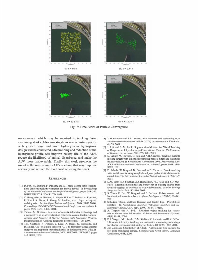
In Figure 7, a series of images represent the conver-

gence of particles while tracking the tagged shark. In 7(a),

the initial time step, the particles are randomly distributed

throughout an L meter by L meter square area centered

around the initial location of the AUV. The second image,

7(b), shows the beginning of particle convergence after a

single acoustic signal is picked up by the hydrophones. The

ambiguity in the sign of α can be observed here by the

fact that particles are into two symetrical groups, one on



(a) (b)

Fig. 5: Tracking a tagged AUV: In (a), the trajectories of the tracking AUV, the tagged AUV2, and the estimated AUV2 are

shown. In (b), the error, standard deviation, and Lotek signal rate of the same experiment are shown.

(a) (b)

Fig. 6: Tracking a tagged shark: In (a), the trajectories of the tracking AUV, the tagged shark, and the estimated shark are

shown. In (b), the standard deviation, and Lotek signal rate of the same experiment are shown.

each side of the AUV. The third image, 7(c), depicts an

instance when the AUV has rotated enough so that only one

of the rays cast by the current bearing measurement (+Z αor -Z α) overlap with one of the existing particle groups.

This geometric overlap leads to appropriate weighting of

particles and convergence to a single accurate location. After

a few more signals from the tag, and only 32 seconds after

the initialization, the particles have consolidated into a tight

distribution in 7(d).

These four images demonstrate the convergence that oc-

curred during each experiment. The particles continually

spread out through propagation, then were weighted and re-

sampled after a Lotek measurement was obtained. It was a

repeated cycle of expansion and contraction, with frequent

contractions during a higher Lotek signal rate.

VII. CONCLUSIONS & FUTURE WORK

A state estimation method has been developed to enable

tracking and following of a tagged sharks. The state estimator

uses a Particle Filtering algorithm containing propagation

and correction steps which control the movement of theparticles. This filtering algorithm has been proven accurate

through testing by localizing a stationary tag, tracking a

tagged AUV, and a tagged shark. While tracking a second

tagged AUV, the average error during the tracking was 41.73

meters, with a minimum value of 0.85 meters. A shark was

continually tracked for a period of 1 hour and 41 minutes,

thus validating this real system.

In the future, the tag signal strength may be calibrated

with both an external sensor system as well as with the

Lotek system in place. This could provide valuable range



(a) t = 0.0 s (b) t = 2.54 s

(c) t = 13.92 s (d) t = 32.37 s

Fig. 7: Time Series of Particle Convergence

measurement, which may be required in tracking faster

swimming sharks. Also, investigations into acoustic systems

with greater range and more hydrodynamic hydrophonedesign will be conducted. Streamlining and reduction of the

hydrophone profile will improve battery life of the AUV,

reduce the likelihood of animal disturbance, and make the

AUV more manuverable. Finally, this work promotes the

use of collaborative multi-AUV tracking that may improve

accuracy and reduce the likelihood of losing the shark.

REFERENCES

[1] D. Fox, W. Burgard, F. Dellaert, and S. Thrun. Monte carlo localiza-tion: Efficient position estimation for mobile robots. In Proceedingsof the National Conference on Artificial Intelligence, pages 343–349.JOHN WILEY & SONS LTD, 1999.

[2] C. Georgiades, A. German, A. Hogue, H. Liu, C. Prahacs, A. Ripsman,R. Sim, L.A. Torres, P. Zhang, M. Buehler, et al. Aqua: an aquaticwalking robot. In Intelligent Robots and Systems, 2004.(IROS 2004).Proceedings. 2004 IEEE/RSJ International Conference on, volume 4,pages 3525–3531. IEEE, 2004.

[3] Thomas M. Grothues. A review of acoustic telemetry technology anda perspective on its diversification relative to coastal tracking arrays.Tagging and Tracking of Marine Animals with Electronic Devices,Diversification of Acoustic Telemetry Technology:77–90, 2009.

[4] T.M. Grothues, J. Dobarro, J. Ladd, A. Higgs, G. Niezgoda, andD. Miller. Use of a multi-sensored AUV to telemeter tagged atlanticsturgeon and map their spawning habitat in the hudson river, USA. In

Autonomous Underwater Vehicles, 2008. AUV 2008. IEEE/OES , pages1–7. IEEE, 2008.

[5] T.M. Grothues and J.A. Dobarro. Fish telemetry and positioning froman autonomous underwater vehicle (AUV). Instrumentation ViewPoint ,(8):78, 2009.

[6] J. Rife and S. M. Rock. Segmentation Methods for Visual Trackingof Deep-Ocean Jellyfish using a Conventional Camera. IEEE Journalof Oceanic Engineering, 28(4):595–608, 2003.

[7] D. Schulz, W. Burgard, D. Fox, and A.B. Cremers. Tracking multiplemoving targets with a mobile robot using particle filters and statisticaldata association. In Robotics and Automation, 2001. Proceedings 2001

ICRA. IEEE International Conference on, volume 2, pages 1665–1670.IEEE, 2001.

[8] D. Schulz, W. Burgard, D. Fox, and A.B. Cremers. People trackingwith mobile robots using sample-based joint probabilistic data associ-ation filters. The International Journal of Robotics Research, 22(2):99,2003.

[9] D.W. Sims, E.J. Southall, A.J. Richardson, P.C. Reid, and J.D. Met-calfe. Seasonal movements and behaviour of basking sharks fromarchival tagging: no evidence of winter hibernation. Marine EcologyProgress Series, 248:187–196, 2003.

[10] S. Thrun, D. Fox, W. Burgard, and F. Dellaert. Robust monte carlo

localization for mobile robots. Artificial Intelligence, 128(1-2):99–141,2001.

[11] Sebastian Thrun, Wolfram Burgard, and Dieter Fox. Probabilisticrobotics. In Probabilistic Robotics (Intelligent Robotics and Au-tonomous Agents), USA, sept. 2005. The MIT Press.

[12] A. Treptow and A. Zell. Real-time object tracking for soccer-robots without color information. Robotics and Autonomous Systems,48(1):41–48, 2004.

[13] F.A. Voegeli, M.J. Smale, D.M. Webber, Y. Andrade, and R.K. O’Dor.Ultrasonic telemetry, tracking and automated monitoring technologyfor sharks. Environmental Biology of Fishes, 60(1):267–282, 2001.

[14] Jun Zhou and Christopher M. Clark. Autonomous fish tracking byrov using monocular camera. Computer and Robot Vision, CanadianConference, 0:68, 2006.

Tracking a Leopard Shark With an AUV

Documents

Transcript of Tracking a Leopard Shark With an AUV