Tracer study of mixing and transport in the upper Hudson … Schlosser, and Ho 1 Tracer study of...

Caplow, Schlosser, and Ho 1

Tracer study of mixing and transport in the upper Hudson River with multiple dams. *Theodore Caplow1, Peter Schlosser2, and David T. Ho3 1Ph. D. Student, Dept. of Earth & Environmental Engineering, Columbia University, 918 Mudd Building, New

York, NY 10027. *Corresponding author. Email [email protected] Tel: (212) 854-7065 Fax: (212) 854-7081

2Professor, Dept. of Earth & Environmental Engineering, and Professor, Dept. of Earth & Environmental Sciences, Columbia University, New York, NY 10027. Email [email protected] Tel: (212) 854-7065 Fax: (212) 854-7081

3Lecturer, Dept. of Earth & Environmental Sciences, and Research Scientist, Lamont-Doherty Earth Observatory, Columbia University, Palisades, New York, NY 10964. Email [email protected] Tel: (845) 365-8706 Fax: (845) 365-8155


Abstract In October 2001, ca. 0.2 mol of SF6 was injected into the upper Hudson River, a modified natural

channel with multiple dams, at Ft. Edward, NY. The tracer was monitored for 7 days as it moved

ca. 50 km downriver. The longitudinal evolution of the tracer distribution was used to estimate 1-

D advection (9.0 ± 0.2 km d-1) and dispersion (17.3 ± 4.0 m2 s-1) along the river axis.

Comparison of these results to tracer studies on channels without dams suggests that dams

reduce longitudinal dispersion below the value expected in a natural channel with the same

discharge. SF6 loss through air-water gas exchange along the river and at two dams (10.7 m

combined height) was estimated by observing decay in peak concentration. Losses at dams

(approximately 50% per dam) were dominant. The estimated gas exchange at dams was

compared to a simple model adapted from those available in the literature. Small amounts of

tracer were trapped in a canal segment (ca. 5 km long) that parallels the river, where advection

and dispersion were sharply reduced.


Introduction

The evolution of a soluble contaminant or nutrient introduced into a river can be divided into

three successive stages, corresponding to periods of vertical, transverse, and longitudinal mixing,

respectively (Fischer et al. 1979). The third stage, sometimes referred to as the far-field, begins

many river widths downstream of the solute’s source, when vertical and transverse mixing are

essentially complete. The focus of this contribution is the behavior of solutes in the far-field, a

subject of primary concern for estimation of time-of-travel and/or dilution capacity at the

watershed or catchment scale (typically tens or hundreds of km).

Predicting the far-field behavior of contaminants in a river requires flow models, and these

models, whether analytical or numerical, must be calibrated to accurate observations of stream

transport processes. As they affect solutes in the far-field, these processes can be divided into

advection (bulk downstream motion), longitudinal dispersion (mixing), and gas exchange (losses

or gains of solutes across the air-water interface). Here we describe the measurement of

advection, longitudinal dispersion, and gas exchange in a river by means of a deliberately

released tracer, sulfur hexafluoride (SF6).

The experiment covered a 65 km reach of the upper, non-tidal Hudson River between Fort

Edward, NY and Troy, NY, and was conducted between October 17 and 23, 2001. This reach

has been heavily altered from its natural state by addition of a dredged channel, dams, locks, and

canals. A number of industrial facilities and power plants are located along this part of the

Hudson, and a public water supply intake is located near the bottom of the study area (at

Waterford, NY), underscoring the need for an accurate transport model in the event of a chronic


or sudden release of a toxic contaminant. The experiment described here was the first application

of SF6 tracer to the study area, and among the first large-scale applications of SF6 to a dammed

channel. The goal was to provide basic empirical data on transport in the study area while

verifying the SF6 tracer methodology for applications to other, similar riverine environments.

Previous tracer work in rivers has been performed with fluorescent dyes such as Rhodamine (e.g.

Wright and Collings 1964; Lowham and Wilson, Jr. 1971; Atkinson and Davis 2000), although

there is a growing body of literature for the application of SF6 to river studies (e.g. Clark et al.

1994; Clark et al. 1996; Hibbs et al. 1998; Chapra and Wilcock 2000; Ho et al. 2002). SF6 has

several properties that make it preferable to fluorescent dyes for studies of advection and mixing

in rivers on large space and time scales. It is non-toxic, inert, inexpensive, and detectable over a

large concentration range (the technique used here is sensitive over a concentration range of at

least four orders of magnitude from about 10 fmol L-1 to about 100 pmol L-1). SF6 is conservative

in the environment and is only lost from the river through gas exchange with the atmosphere.

Study Conditions The Hudson River flows southward over 500 km from its source in the Adirondack Mountains to

New York Harbor, draining an area of 35,000 km2 (Limburg et al. 1986). The river is navigable

downstream of Fort Edward, NY at kilometer point (kmp) 313, measured axially upstream from

the southern tip of Manhattan. Below the Federal Dam at Troy (kmp 248), the river is tidal, with

bi-directional flow. Above the Federal Dam, the river changes character (Figure 1), becoming a

narrower, shallower stream altered from its natural course by the construction of the Champlain

Canal system. There are six locks between kmp 248 and kmp 313, for a total change in elevation


of 31 m (Erie 2002). Each lock is 13 m wide and 91 m long and is accompanied by a dam and

spillway. Many of the locks are placed at the southern end of man-made canals dug parallel to,

but separate from, the natural river. There are four canals in the study area, all located upstream

of a lock. These canals, which are approximately 30 m wide, are found above lock #6 (~5 km),

lock #5 (~1.5 km), and lock #4 (~0.9 km), and below lock #1 (~0.7 km). The controlling depth

for the canals, locks, and navigable river is 3.7 m (12 feet).

The 25-year mean flow of the Hudson River is 147 m3 s-1 at Ft. Edward and 385 m3 s-1 at Troy

(USGS 2002; EPA 2000). Major tributaries within this reach include the Batten Kill (kmp 293,

average flow 17 m3 s-1), the Hoosic River (kmp 270, average flow 38 m3 s-1), and the Mohawk

River (kmp 250, average flow 160 m3 s-1). The mean flow at Ft. Edward during October 2001

was 53 m3 s-1. This volume was the lowest recorded in the past 25 years and is equivalent to 36%

and 45% of the annual and October means, respectively. This anomaly is expected to have had a

significant effect on rates of advection, dispersion, and gas exchange.

Bathymetry from EPA (2000) was used to estimate the channel width and mean depth at the

injection point, as well as the mean properties for the study reach as a whole. The bathymetry

consists of mean depth and mean width for a grid that is one box wide in the transverse direction,

with a 2 km longitudinal resolution, except between kmp 304 and kmp 313, where the transverse

resolution is 3 boxes and the longitudinal resolution is 1 km. The mean width and depth for the

upper Hudson River are 268 m and 3.1 m, respectively.


Field Methods Measurements of SF6 conducted before the tracer injection indicated a background concentration

of less than 10 fmol L-1 in the upper Hudson River. On October 17, 2001 at 08:30 EST (“day

0.0”; time is measured in elapsed days since injection), approximately 0.2 moles of SF6 were

bubbled into the river midstream at kmp 311 through a porous rubber/polyethylene tubing (7 m

long, 0.6 cm ID, 150 µm pore size). The tubing was wrapped around a metal cylinder attached to

a weight and its depth was controlled at approximately 3 m. Flow was maintained for one

minute. Shortly thereafter, survey of the SF6 patch began, using a boat-mounted, fully automated,

high-resolution sampling and measurement system (Ho et al. 2002). Water from the river was

pumped continuously through a counter-flow membrane contactor, where gases were extracted

and analyzed for SF6 by electron-capture gas chromatography. This equipment takes a

concentration measurement every two minutes. Boat speed during surveys ranged from 3 to 8

knots (5 to 15 km h-1), resulting in a spatial data resolution of 0.2 to 0.5 km along the axis of the

river.

The survey was conducted for seven consecutive days, between 8 am and 6 pm. The SF6 patch

was surveyed either as the boat traversed the patch in a longitudinal direction upriver or

downriver, or from fixed positions as the tracer-tagged water flowed past. In addition to the main

patch, a slug of SF6 trapped in a 5 km canal above lock #6 (kmp 299) was observed for the

duration of the experiment.


Analytical Methods The far-field study of advection and longitudinal dispersion in rivers is often approached via a

one-dimensional (1-D) approximation, in which the width and depth are treated as constants, and

lateral and vertical mixing are neglected (Fischer et al. 1979; Rutherford 1994). This

approximation is justified if the timescale is sufficiently large such that horizontal and vertical

mixing are essentially complete before measurements of longitudinal dispersion are made. If a

tracer injection is used, it is further necessary that the injection be nearly “instantaneous” in

comparison with the timescale of observation.

The transverse scale is much larger than the vertical scale in most rivers, including the upper

Hudson. A test of transverse mixing time against longitudinal measurement interval, if

successful, suffices to justify the 1-D approximation in non-saline rivers (where vertical water

column stratification is assumed to be transient and/or weak). Rutherford (1994) performs this

test by assuming a constant dispersion coefficient and estimating transverse mixing time Tt:

Tt = α B2

Ky

(1)

where B is the mean width of the river (225 m at the injection site), Ky is the transverse

dispersion coefficient, and α is a coefficient defining the well mixed state. According to Fischer

et al. (1979), if α is set to 0.075 then the tracer concentration will be within 10% of its mean

anywhere on the cross-section after an elapsed time of Tt (since injection). The analytical

prediction of Ky remains unsatisfactory to many investigators (e.g. Heard et al. 2001; Boxall and

Guymer 2003) but Ky = 0.6 H u* is an expression commonly used for slightly meandering

channels (Fischer et al. 1979), where H is mean channel depth (2.6 m at the injection site) and u*


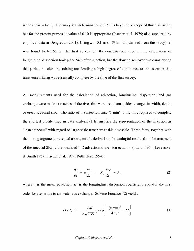
is the shear velocity. The analytical determination of u*/u is beyond the scope of this discussion,

but for the present purpose a value of 0.10 is appropriate (Fischer et al. 1979; also supported by

empirical data in Deng et al. 2001). Using u = 0.1 m s-1 (9 km d-1, derived from this study), Tt

was found to be 65 h. The first survey of SF6 concentration used in the calculation of

longitudinal dispersion took place 54 h after injection, but the flow passed over two dams during

this period, accelerating mixing and lending a high degree of confidence to the assertion that

transverse mixing was essentially complete by the time of the first survey.

All measurements used for the calculation of advection, longitudinal dispersion, and gas

exchange were made in reaches of the river that were free from sudden changes in width, depth,

or cross-sectional area. The ratio of the injection time (1 min) to the time required to complete

the shortest profile used in data analysis (1 h) justifies the representation of the injection as

“instantaneous” with regard to large-scale transport at this timescale. These facts, together with

the mixing argument presented above, enable derivation of meaningful results from the treatment

of the injected SF6 by the idealized 1-D advection-dispersion equation (Taylor 1954; Levenspiel

& Smith 1957; Fischer et al. 1979; Rutherford 1994):

cdx

cKxcu

tc

x λ−∂∂∂

∂∂

2

2

=+ (2)

where u is the mean advection, Kx is the longitudinal dispersion coefficient, and λ is the first

order loss term due to air-water gas exchange. Solving Equation (2) yields:

λ−−−

πν t

tKutx

tKAMtxc

xx 4)(exp

4=),(

2

(3)


where v is the specific volume of the gas tracer, M is the mass of trace gas injected and A is the

mean cross-sectional area of the river (all three of these values are constant for the purposes of

this analysis). One method for determining Kx from experimental data is via the “change of

moment” (Fischer et al. 1979; Rutherford 1994):

−σ−σ=

σ=12

21

22

2

21

21

ttdtdK x (4)

where 2

1σ and 22σ are the variances (second moments) of the tracer distributions at times t1 and

t2 respectively. Equation (4) is applied between SF6 surveys, taken on different days, to calculate

a single mean value of Kx for the temporal and spatial extent of the study.

The value of σ2 for the SF6 patch from a single survey was estimated by fitting Gaussian curves

(minimizing chi square) to two longitudinal profiles of the patch, taken very close together in

time but in opposite directions, and averaging σ2 from both curve fits. Bi-directional profiles

were used to reduce uncertainty and to remove any possible bias from lag or memory effects in

the sampling equipment. The maximum discrepancy between observed values for σ2 within a

single pair of bi-directional profiles was 10%. Four profiles suitable to the fitting of Gaussian

curves were collected (a bi-directional pair on both day 3 and day 4). In addition, three pairs of

bi-directional profiles were collected in the canal above lock #6 (on days 2, 3, and 4) and

analyzed for dispersion by the same method. This approach corresponds to the simplest

analytical model, which is symmetrical and constant (i.e. Fickian) dispersion. More complex

models are also in use, in particular the “dead zone model”, attributed to Hays (1966), which

accounts for an asymmetrical tracer patch (with longer upstream tail) by proposing that portions

of the river, or its bed, retard pockets of tracer while the rest is advected downstream. The SF6


profiles from the present study display a slight asymmetry, but the upstream tails were truncated

by dams, as it was not possible to survey continuously past these structures.

Equation (4) requires a set of observations of σ2, each of which is assumed to be synoptic. The

data were normalized to a synoptic form by shifting each data point a small distance, determined

by the mean advection (u) and the elapsed time between data collection at that point and the time

when the peak SF6 concentration was observed. The maximum shift was < 0.1 σ, where σ2 was

the variance of the profile. Dispersion during the profile itself was neglected.

Loss of SF6 via gas exchange at the air-water interface was investigated by examining the

decline, between successive observations, of the peak SF6 concentration in the tracer patch. (This

approach was chosen because the collection of complete SF6 inventories, from which losses

could be directly calculated, was only possible on one occasion due to interference from locks

and dams.) Fischer et al. (1979) observed that in a 1-D system with symmetrical Fickian

dispersion and no losses the evolution of the peak concentration (cp) is proportional to the

inverse of the square root of the elapsed time since injection: cp ∝ t −0.5. This conclusion is

evident from a consideration of Equation (3) at the peak (x = ut) with no losses (λ = 0). If such a

tracer peak is measured at two times t1 and t2 then it follows directly that:

5.0

2

1

1

2 =

tt

cc

p

p (5)

where cp1 and cp2 are the peak tracer concentrations at times t1 and t2, respectively. For the

purpose of evaluating net tracer loss from peak concentration data it is useful to introduce f12, the

fraction of tracer which is removed from the water between times t1 and t2:


5.0

1

2

1

212 1

−=

tt

cc

fp

p (6)

Equation (6) does not depend upon the actual form or temporal distribution of the losses,

provided that the tracer profiles at both t1 and t2 are well represented by the Gaussian curves

described by Equation (3), and that Equation (5) is valid. Jobson (1997) performed regression

analysis on a heterogeneous data set of 422 cross-sections from 60 rivers in the United States and

found that cp ∝ t −0.89, whereas various other investigators have found values for the exponent

ranging from −0.7 to −1.0. This increase in longitudinal dispersion above the intensity suggested

by the Fickian model is usually ascribed to additional modes of mixing (e.g. dead zones). The

simpler relationship cp ∝ t −0.5 was adopted here for two reasons. First, this relationship maintains

consistency with the Fickian model used for the dispersion calculations, which appears the most

generic model for observing first-order transport effects under these conditions. Second, this

relationship matches the observed decay of the SF6 peak in an inter-dam reach of the study area

about 35 km downstream of the injection point (see Results), indicating that the impact of patch

asymmetry was minor for the experiment described. Considering the potential for gas exchange

losses over this reach, it appears the appropriate exponent relating cp and t may have been even

higher than −0.5, a result at odds with the aforementioned regressions from the literature.

Equation (6) was applied to data from three surveys where cp was well defined (one each on days

2, 3, and 5) to evaluate the effect of dams upon SF6 losses to the atmosphere. A large increase in

gas exchange is expected at dams, due to the extreme turbulence, bubble invasion, and vertical

mixing that occur downstream (e.g. Cirpka et al. 1993; Asher et al. 1996). The reach between the


survey locations for days 2 and 3 is regular in form and unobstructed. Two dams (4.8 m and 5.9

m; Erie 2002) are located between the survey locations for days 3 and 5.

A minor correction was made to f12 to account for dilution from tributaries (20% over this reach;

EPA 2000). This dilution was assumed to cause a linear reduction in cp as a function of distance

downstream from the injection point.

Results SF6 was measured in the river until day 6, at which time the signal of the main patch had

decreased to nearly undetectable levels. The downstream motion and longitudinal spreading of

the SF6 peak is well represented in the data, despite irregularities in the river (locks and dams).

Results from a longitudinal profile taken on day 3 (Figure 2) clearly indicate small slugs of tracer

trapped in canals at locks #5 and #6, as well as the main tracer patch further downstream. The

SF6 mass inventory in the main channel on day 3 was estimated as 1.5 ± 0.15 mmol,

approximately 1% of the estimated amount injected. Based on prior experience (Ho et al. 2002)

and the relatively shallow depth of the river, it is expected that the majority of the SF6 injected

(more than 90%) escaped from the water as bubbles during the injection process. Additional

reduction in the SF6 inventory is attributed to air-water gas exchange, including losses at dams.

Advection Observations of the peak concentrations within the tracer patch enabled estimates of the mean

advection rate (Figure 3). Mean advection over a 42 km reach (kmp 306 to kmp 264) was 9.0 ±

0.2 km d-1 (0.104 ± 0.002 m s-1), corresponding to a transit time of seven days from Fort Edward


to Troy (65 km) if the same rate is applied to the remaining 23 km. Multiplying the observed

advective rate by the cross-sectional area of the river at the injection point just south of Ft.

Edward (585 m2) yields a flow rate of 61 m3 s-1. This rate is in reasonable agreement with the

rate of 53 m3 s-1 reported by the USGS at Ft. Edward for the whole of October 2001.

Dispersion

On day 2 (at kmp 289) and day 3 (at kmp 280) it was possible to obtain pairs of bi-directional

profiles of the main body of the SF6 patch suitable for extracting the variance (σ2) by fitting a

Gaussian curve to each profile (Figure 4). The variances for each pair were averaged and the

longitudinal dispersion coefficient (Kx) was calculated using Equation (4), resulting in values of

15.7 ± 2.0 m2 s-1 for day 2.3 (55 h from injection) and 19.0 ± 2.4 m2 s-1 for day 3.2 (77 h from

injection). The average Kx was 17.3 ± 4.0 m2 s-1 (1.50 ± 0.35 km2 d-1). The data supporting this

value were collected along the top 31 km of the study reach. Downstream of kmp 280, no further

determinations of σ2 were possible. In this lower reach (kmp 280 to kmp 248), significant

changes in the character of the channel or the volume of the flow are not evident, suggesting that

the estimate of Kx obtained from the upper reach should be a reasonably good approximation for

this region as well.

Gas Transfer Results from applying Equation (6) to three successive pairs of peak tracer concentration

measurements are shown in Table 1. According to these limited results, the dams are the major

cause of SF6 tracer loss in the study area, and SF6 losses between dams are a very small term in

the overall loss rate. No detectable loss was measured over a 9 km reach (measurements were 23


h apart) between kmp 289 and kmp 280 that contained no dams, but a 72% loss was recorded

over a 14 km reach (measurements were 39 h apart) between kmp 280 and kmp 266 that

contained two dams.

SF6 trapped in the canal above lock #6 The mean cross sectional area of the canal above lock #6 was estimated (field observations) to be

90 ± 25 m2. The total SF6 inventory in this canal was calculated from a profile taken on day 3

(3.1 days after injection) as 72 ± 13 µmol (using a cross-sectional area of 90 m2). This inventory

is approximately 5% of the inventory measured in the main channel on day 3. Tracer mass in the

canal was also calculated from profiles on days 2 and 4 (Figure 5), but the data do not show a

significant trend that would enable an estimate of gas transfer rate. Gaussian curves were fitted to

each profile (Figure 5). Advection was determined from the peaks of the curve fits to be 0.7 ±

0.06 km d-1. Longitudinal dispersion (Kx) in the canal was estimated as 1.2 ± 0.3 m2 s-1 (0.11 ±

0.025 km2 d-1) by a least square fit of σ2 versus time, corresponding to the relationship predicted

by Equation (4).

Discussion The advection rate along the measured reach was constant within measurement errors (Figure 3).

Intuitively, this result seems surprising in view of the irregularities along this reach. To examine

the uniformity of flow per unit area, cross-sectional area and average contributions from

tributaries were obtained from EPA (2000) and plotted versus river kilometer (Figure 6). The

plot illustrates that as tributaries and run-off enter the main stem of the river, the cross-sectional

area increases to accommodate the additional flow, producing a near-constant mean velocity.


Deng et al. (2001) compile a set of 73 empirical data points containing longitudinal dispersion

coefficient, width, depth, mean velocity, and shear velocity, drawn from studies of 29 different

rivers in the United States. The data set, derived primarily from dye tracer studies, contains 58

data points from Seo and Cheong (1998) and 15 data points from Rutherford (1994). These

measurements were made on reaches without dams. As no similar data set exists for rivers with

dams, the Deng et al. (2001) data is used here as a means for comparing the upper Hudson River

to channels without dams.

The median and mean Kx for all 73 data points are 40.5 and 132 m2 s-1, respectively. 77% of the

Kx measurements were higher than that found for the upper Hudson River. These data were used

to construct plots of Kx versus nominal discharge (width × depth × mean velocity), mean

velocity, and nominal cross-sectional area (width × depth), respectively (Figure 7). Two upper

Hudson River data points were added to the plots: the solid circles represent the results of the

October 2001 SF6 study. The solid triangles (“normal-flow prediction”) represent the upper

Hudson River after applying a correction for the anomalously low flow conditions prevalent

during the experiment. An increase by a factor of 2.4 in the discharge of the upper Hudson River

during the study would correspond to 25-year mean conditions. Hibbs et al. (1998), on the basis

of earlier work by McQuivey and Keefer (1974), suggest that a linear relationship between Kx

and discharge is successful within ± 80% in natural streams if at least one measured value of Kx

has already been found. Applying a linear factor of 2.4 to Kx in the upper Hudson River results in

an increase from 17 to 42 m2 s-1. It is further assumed, for the purposes of this prediction, that the

cross-sectional area would not change significantly with discharge (the dams control cross-


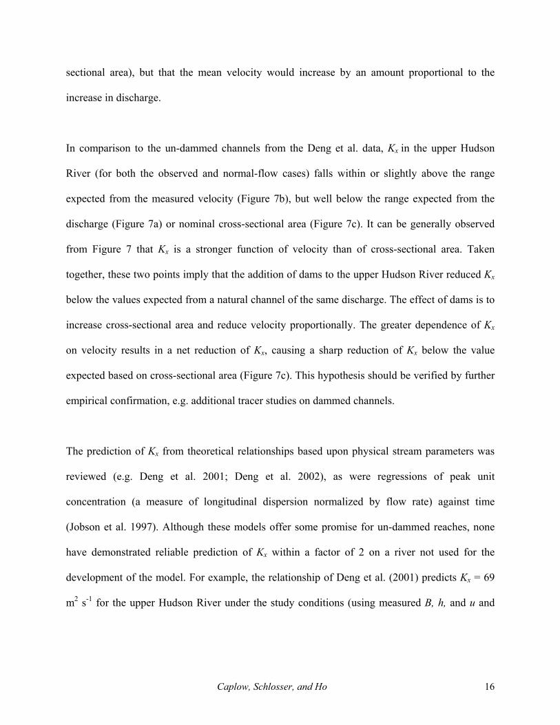
sectional area), but that the mean velocity would increase by an amount proportional to the

increase in discharge.

In comparison to the un-dammed channels from the Deng et al. data, Kx in the upper Hudson

River (for both the observed and normal-flow cases) falls within or slightly above the range

expected from the measured velocity (Figure 7b), but well below the range expected from the

discharge (Figure 7a) or nominal cross-sectional area (Figure 7c). It can be generally observed

from Figure 7 that Kx is a stronger function of velocity than of cross-sectional area. Taken

together, these two points imply that the addition of dams to the upper Hudson River reduced Kx

below the values expected from a natural channel of the same discharge. The effect of dams is to

increase cross-sectional area and reduce velocity proportionally. The greater dependence of Kx

on velocity results in a net reduction of Kx, causing a sharp reduction of Kx below the value

expected based on cross-sectional area (Figure 7c). This hypothesis should be verified by further

empirical confirmation, e.g. additional tracer studies on dammed channels.

The prediction of Kx from theoretical relationships based upon physical stream parameters was

reviewed (e.g. Deng et al. 2001; Deng et al. 2002), as were regressions of peak unit

concentration (a measure of longitudinal dispersion normalized by flow rate) against time

(Jobson et al. 1997). Although these models offer some promise for un-dammed reaches, none

have demonstrated reliable prediction of Kx within a factor of 2 on a river not used for the

development of the model. For example, the relationship of Deng et al. (2001) predicts Kx = 69

m2 s-1 for the upper Hudson River under the study conditions (using measured B, h, and u and


assuming u*/u = 0.1). Despite advances in analytical prediction, tracer studies continue to hold

value in the determination of longitudinal dispersion, particularly in dammed channels.

The relatively slow mixing and advection in the canals, together with expected seasonal variance

in these properties (as a function of boat traffic and lock cycling rate), is of significance for spill

forecasting and modeling. The canals appear to have the capacity to trap small amounts of

solutes from the main channel for long periods of time (days to weeks). It follows that

contaminants introduced directly into the canals would persist for a much longer time, and at

higher concentrations, than they would if spilled in the main channel. Five days into the

experiment, parcels of water containing significant amounts of SF6 were still working their way

through the canal above lock #6 (only several km south of the injection point). At this time the

main patch had passed 30 km downriver and peak concentrations there were an order of

magnitude smaller than in the lock #6 canal.

Predicted Gas Transfer at Dams Erie (2002) tabulated the change in river elevation at each lock on the upper Hudson; these drops

are good estimates for the heights of the dams. Based upon a review of the literature, a rough

model was developed (Appendix I) to calculate the loss of SF6 over the dams of the upper

Hudson River as a function of dam height, h, and specific flow, q (flow per unit of dam width).

The net flow rate at these dams was calculated as 76 m3 s-1 by adding 24% tributary dilution

(EPA 2000) to the flow determined at the injection site from the measured advection. Three

values for q were examined, corresponding to 50%, 100%, and 200% of the net flow rate divided

by an approximate mean dam width of 200 m (observed from satellite photos). Predicted values

for f12 from the model (75% − 86%) are compared to the measured (72%) cumulative losses over


the two dams spanned by the tracer patch peak measurements on days 3 and 5 (Table 2). The

model developed here is a rough approximation which appears to capture the major effects. A

dedicated experiment would be necessary to understand all of the factors affecting gas exchange

over dams of this type.

Acknowledgements We thank Nicholas Santella and Fred Stuart for assistance in the field. Special thanks to John

Lipscomb, boat captain for Riverkeeper, whose expert handling of his vessel ensured a smooth

and successful field project. The authors are grateful for the valuable comments of three

anonymous reviewers. Funding was provided by a generous grant from the Dibner Fund and by

the Lamont Investment Fund. LDEO contribution ####.


Appendix I. Model for SF6 loss over dams on the Upper Hudson River

Both Gulliver et al. (1998) and Cirpka et al. (1993) present predictive relationships found in the

literature for gas transfer efficiency as a function of physical parameters of flow over hydraulic

structures (dams, weirs, spillways, cascades and gates). It is standard in these relationships to

employ the dependent variables E and r:

ed

eu

CCCCr

rE

−−=

−= 11

(A1)

where E is the gas transfer efficiency (achieved gas transfer divided by total potential gas

transfer), r is termed the excess ratio (or deficit ratio, depending upon the gas), Ce is the

equilibrium gas concentration, and Cu and Cd are the gas concentrations upstream and

downstream of the structure, respectively.

According to Cirpka et al. (1993) and Gulliver et al. (1998), gas transfer at hydraulic structures

of moderate size (1 to 10 m high) is dominated by diffusion across the surface of air bubbles that

are entrained as the falling water enters the catch basin below the dam. The formation and

division of bubbles greatly magnifies the available surface area for gas transfer, while the

physical turbulence in the zone where these bubbles rise to the surface accelerates dispersion

away from the bubble-water interface. This process can be parameterized in a number of ways.

Gulliver et al. (1998) investigated 12 formulations and settled on the following classical

relationship, originally formulated by Avery and Novack (1978), as the best predictor for oxygen

invasion at weirs:


ν8

104.2111

41

2

3

53.078.15,2

qeRqghFr

eRFrE weirO

=

=

×+−= −

(A2)

where weirOE ,2 is the gas transfer efficiency for oxygen, Fr and Re are the Froude and Reynolds

numbers of the jet, respectively, g is the gravitational constant, h is the drop over the weir, q is

the specific flow per horizontal length of weir (m2 s-1), and ν is the kinematic viscosity of the

water (SI units are used for all variables). This relationship was developed for water at 15 ˚C.

Over 95% of upper Hudson River water temperature observations from the October 2001 study

were within ± 2 ˚C of 15 ˚C.

In order to apply Equation (A2) to SF6, the difference in molecular properties between O2 and

SF6 must be considered. Cirpka et al. (1993) show that both O2 and SF6 have sufficiently high

Henry’s Law constants to ensure that gas exchange is limited by the liquid side of the air-water

interface, even inside of a rising bubble of entrained air. Their formulation for the excess ratio, r,

for gases sharing this characteristic takes the form:

r =1+Y D (A3)

where Y is a constant specific to the flow and to the weir, and D is the aqueous molecular

diffusion coefficient. Designating RD = DSF6DO2

(the ratio of the molecular diffusion

coefficients of SF6 and O2) and using Equations (A1) and (A3), the SF6 transfer efficiency can be

expressed as a function of EO2 and RD:

( )11

26

11−−

−+=D

OSF R

EE (A4)


In all calculations, RD is taken as 0.53.

As written, Equation (A2) is intended for oxygen invasion, and therefore Equation (A4) is an

estimate for the invasion of SF6, rather than its evasion (loss). Asher et al. (1996) demonstrate

that gas transfer in bubble plumes should not be assumed to be symmetrical with regard to

invasion or evasion of a particular gas. Invasive transfer includes a contribution from a certain

fraction of bubbles that will collapse completely before surfacing, adding gas to the water in a

non-equilibrium process. Evasive transfer lacks this term and therefore will be over-estimated by

parameterizations developed from observations of invasion. Asher et al. (1996) point out that this

asymmetry will increase with decreasing solubility (because the contribution of a collapsed

bubble becomes more significant relevant to the contribution of a surfacing bubble), and also

suggest that evasion for highly insoluble gases such as SF6 will be further reduced (relative to

invasion) by depletion of dissolved gas in the immediate vicinity of the rising bubble plume.

Asher et al. (1996) conducted experiments in a seawater tank, revealing that under sufficiently

bubbly conditions, transfer efficiency for SF6 invasion could be up to 50% greater than for SF6

evasion. However, their results also suggest that the equations derived here from O2 data can be

expected to underestimate SF6 invasion by roughly the same amount that they overestimate SF6

evasion; thus the total overestimate of SF6 loss from a river dam is expected to be substantially

less than 50%. The current model is intended to illustrate the effect of various parameters (such

as dam height) on gas exchange while providing no more than a crude estimate of the magnitude.

Lacking methodical studies of SF6 loss over dams of the type encountered in the upper Hudson


River, any additional precision would be conjectural at this point. Accordingly, the model

neglects asymmetry with regard to direction.

Equation (A2) was originally derived for sharp crested weirs with a separated free jet of water.

On the upper Hudson River, the majority of dams were observed to be of the rounded crest type

(ogee crest), with an inclined spillway and attached flow. Based on 54 small dams, Butts and

Evans (1983) developed a predictive equation for oxygen deficit ratio r that included a shape

parameter. As presented in Tang et al. (1995), their equation has the form:

),,(1 Thafbr •+= (A5)

where a is a factor to account for water quality, h is dam height, T is temperature, and the shape

parameter b ranges from 0.6 for a broad-crested dam to 1.05 for a sharp-crested weir. In order to

convert transfer efficiencies derived from the sharp-crested weir equation (A2) for use with the

broad crested dams of the upper Hudson River, consider two dams of equal height under equal

conditions, for which ),,( Thaf is a constant, Z:

bZr +=1 (A6)

Comparing this relationship with the top part of Equation (A1) reveals:

1

11 −

+=

ZbE (A7)

This equation holds for a dam of either shape. To convert from a sharp weir to a broad crest:

Ebroad

Eweir

= 1Zbbroad

+1

1Zbweir

+1

−1

(A8)

which after manipulation yields:

1

111−

+

−=

weirbroad

weirbroad Eb

bE (A9)


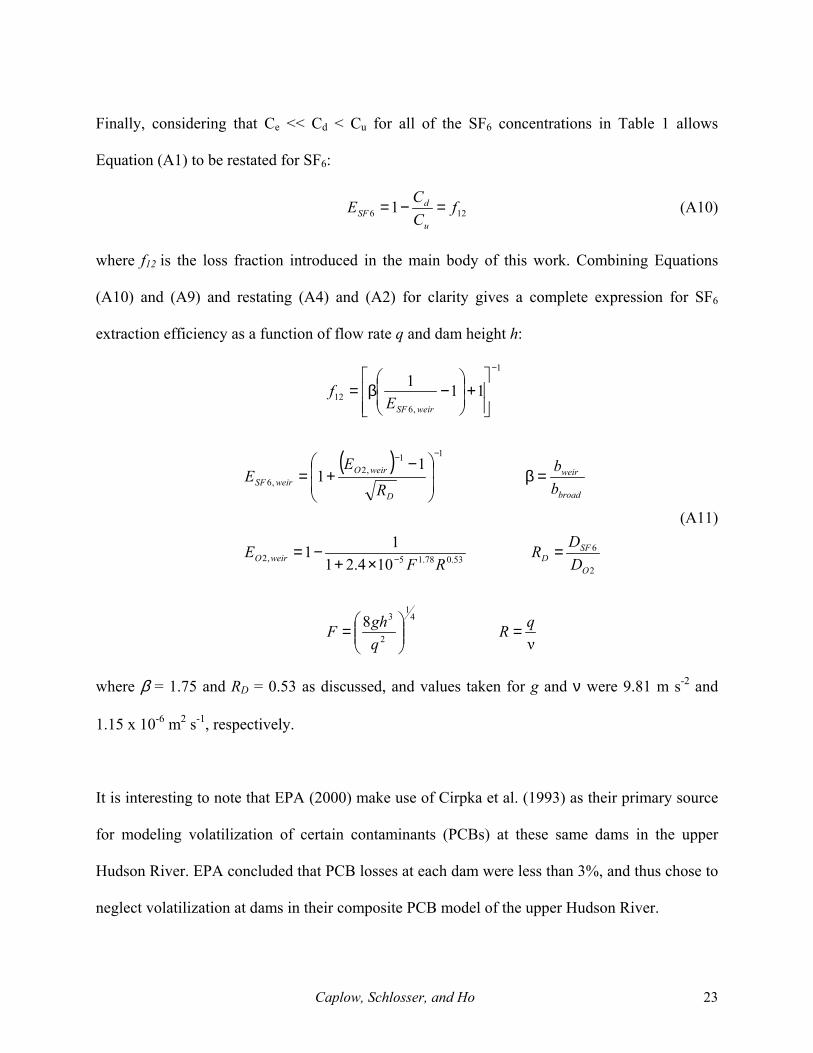
Finally, considering that Ce << Cd < Cu for all of the SF6 concentrations in Table 1 allows

Equation (A1) to be restated for SF6:

126 1 fCCE

u

dSF =−= (A10)

where f12 is the loss fraction introduced in the main body of this work. Combining Equations

(A10) and (A9) and restating (A4) and (A2) for clarity gives a complete expression for SF6

extraction efficiency as a function of flow rate q and dam height h:

( )

ν8

104.2111

11

111

41

2

3

2

653.078.15,2

11,2

,6

1

,612

qRqghF

DDR

RFE

bb

R

EE

Ef

O

SFDweirO

broad

weir

D

weirOweirSF

weirSF

=

=

=×+

−=

=β

−+=

+

−β=

−

−−

−

(A11)

where β = 1.75 and RD = 0.53 as discussed, and values taken for g and ν were 9.81 m s-2 and

1.15 x 10-6 m2 s-1, respectively.

It is interesting to note that EPA (2000) make use of Cirpka et al. (1993) as their primary source

for modeling volatilization of certain contaminants (PCBs) at these same dams in the upper

Hudson River. EPA concluded that PCB losses at each dam were less than 3%, and thus chose to

neglect volatilization at dams in their composite PCB model of the upper Hudson River.


Appendix II. References Asher, W. E., Karle, L. M., Higgins, B. J., Farley, P. J., Monahan, E. C., and Leifer, I. S., (1996).

“The influence of bubble plumes on air-seawater gas transfer velocities.” J. Geophy. Res., 101(C5), 12027-12041.

Atkinson, T.C. and Davis, P. M., (2000). “Longitudinal dispersion in natural channels: 1. Experimental results from the River Severn, UK.” Hydrol. Earth Syst. Sci., 4(3), 345-353.

Boxall, J. B., and Gumer, I. (2003). “Analysis and prediction of transverse mixing coefficients in natural channels.” J. Hydraulic Engrg. 129(2), 129-139.

Butts, T. A., and Evans, R. L. (1983). “Small stream channel dam aeration characteristics.” J. Environ. Engrg., 109(3), 555-573.

Chapra, S. C., and Wilcock, R. J. (2000). “Transient storage and gas transfer in lowland stream.” J. Environ. Engrg., 126(8), 708-712.

Cirpka, O., Reichart, P., Wanner, O., Muller, S. R., and Schwarzenback, R. P. (1993). “Gas exchange at river cascades: field experiments and model calculations.” Environ. Sci. Technol., 27(10), 2086-2097.

Clark, J. F., Schlosser, P., Stute, M., and Simpson, H. J. (1996). “SF6-3He tracer release experiment: a new method of determining longitudinal dispersion coefficients in large rivers.” Environ. Sci. Technol., 30(5), 1527-1532.

Clark, J. F.; Wanninkhof, R.; Schlosser, P.; Simpson, H. J. (1994). “Gas exchange rates in the tidal Hudson River using a dual tracer technique.” Tellus, B46(4), 274-285.

Deng, Z., Singh, V. P., and Bengtsson, L. (2001). “Longitudinal dispersion coefficient in straight rivers.” J. Hydraulic Engrg., 127(11), 919-927.

Deng, Z., Bengtsson, L., Singh, V. P., and Adrian, D. D. (2002). “Longitudinal dispersion coefficient in single channel streams.” J. Hydraulic Engrg., 128(10), 901-916.

EPA (2000) Revised Baseline Modeling Report: Hudson River PCBs Reassessment RI/FS EPA, New York. Available online at http://www.epa.gov/hudson/reports.htm, viewed 02/04/02.

Erie Lock 2 Employees (2002). http://www.yolles.net/canals/pagef.htm, web site viewed 01/20/02.

Fischer, H. B., List, E. J., Imberger, J., Koh, R. C. Y., and Brooks, N. H. (1979). Mixing in inland and coastal waters, Academic Press, New York.

Gulliver, J. S., Wilhelms, S. C., and Parkhill, K. L. (1998). “Predictive capabilities in oxygen transfer at hydraulic structures.” J. Hydraulic Engrg., 124(7), 664-671.

Hays, J. R. (1996). “Mass transport phenomena in open channel flow.” Ph.D. dissertation, Vanderbilt University, Nashville, Tennessee.

Heard, S. B, Gienapp, C. B., Lemire, J. F., Heard, K. S. (2001). “Transverse mixing of transported material in simple and complex stream reaches.” Hydrobiol. 464, 207-218.

Hibbs, D. E., Perkhill, K. L., and Gulliver, J. S. (1998). “Sulfur hexafluoride gas tracer studies in streams.” J. Environ. Engrg., 124(8), 752-760.

Ho, D.T., Schlosser, P. and Caplow, T. (2002). “Determination of longitudinal dispersion coefficient and net advection in the tidal Hudson River with a large-scale, high resolution SF6 tracer release experiment.” Envir. Sci. Technol., 36, 3234-3241.

Hohman, M. S., and Parke, D. B. (1969) in Hudson River Ecology, Hudson River Valley Commission of New York, Albany, NY, 60-81.

Jähne, B., Munnich, K. O., Bosinger, R., Dutzi, A., Huber, W., and Libner, P. J. (1987). “On the parameters influencing air-water gas exchange.” J. Geophys. Res. 92(C2), 1937-1949.


Jobson, H. E. (1997). “Predicting travel time and dispersion in rivers and streams.” J. Hydraulic Engrg. 123(11), 971-978.

Kashefipour, S. M. and Falconer, R. A. (2002). “Longitudinal dispersion coefficients in natural channels.” Water Research, 36, 1596-1608.

Levenspiel, O. and Smith, W. K. (1957). “Notes on the diffusion-type model for the longitudinal mixing of fluids on flow.” Chem. Engng. Sci., 6, 227-233.

Limburg, K. E., Moran, M. A., and McDowell, W. H. (1986). The Hudson River Ecosystem, Springer-Verlag, New York.

Lowham, H. W., and Wilson, Jr., J. F. (1971) "Preliminary results of time-of-travel measurements on Wind/Bighorn River from Boysen Dam to Greybull, Wyoming.", U. S. Geological Survey Report.

McQuivey, R. S., and Keefer, T.N. (1974). “Simple method for predicting dispersion in streams.” J Envir. Engrg. Div., ASCE, 100(4), 997-1011.

Rutherford, J. C. (1994) River mixing, Wiley, New York. Seo, I. W., and Cheong, T. S. (1998). “Predicting longitudinal dispersion coefficient in natural

streams.” J. Hydraulic Engrg., 124(1), 25-32. Tang, N. H., Nirmalakhandan, N., and Speece, R. E. (1995). “Weir aeration: models and unit

energy consumption.” J Envir. Engrg., 121(2), 196-199. Taylor, G. I. (1954). “Dispersion of matter in turbulent flow through a pipe.” Proc. Royal Soc.

Ser. A, 223, 446-468. USGS (2002) http://water.usgs.gov, web site viewed 02/04/02. Wright, R. R., and Collings, M. R. (1964). "Application of fluorescent tracing techniques to

hydraulic studies." J. Amer. Water Works Assoc., 56, 748-755.


Appendix III. Notation A = cross-sectional river area;

B = mean river width;

Cd = downstream concentration;

Ce = equilibrium concentration;

Ci = initial concentration;

Cu = upstream concentration;

D = aqueous molecular diffusion coefficient;

E = gas transfer efficiency;

Fr = Froude number;

H = mean river depth;

Kx = longitudinal dispersion coefficient;

Ky = transverse dispersion coefficient;

M = mass of trace gas injected;

Re = Reynolds number;

RD = ratio of molecular diffusion coefficients;

T = temperature;

Tt = transverse mixing time;

Y, Z = arbitrary constants;

a = water quality factor;

b = dam shape factor;

c = tracer concentration;

cp = peak tracer concentration;

f12 = fraction of tracer lost between observations;

g = gravitational constant;

h = dam height;

q = flow per unit width;

r = excess ratio;

t = time;

t0 = injection time;


u = mean advective velocity;

u* = bed shear velocity;

v = specific volume;

x = distance traveled;

α = coefficient defining complete transverse mixing;

β = ratio of dam shape factors;

∆c = air-water concentration difference;

λ = gas exchange loss term;

ν = kinematic viscosity; and

σ2 = variance (second moment) of a distribution.


Table 1: SF6 losses with and without dams, calculated from peak concentrations.

Modeled Peaks, fmol L-1 Day kmp σpred,

kma Dispersion only

Dispersion & Dilution

Actual Peak, fmol L-1 f12

t2 - t1, days

# of dams 1 ↔ 2

2.31 288.8 2.63 281

3.21 279.9 3.10 239 223 222 0.00 0.9 0

4.90 266.1 3.83 193 155 43b 0.72 1.7 2 aThe values given for σ are not the measured values; these are expected values based on the measured mean Kx. This approach is necessary to apply the peak inventory estimate evenly to locations where σ could not be measured directly, as well as those where it could be measured. bThe peak was tentatively identified twice more shortly after this time. Both measurements were similar to this one. Following these measurements, the patch crossed another dam and signal levels fell below the detection limit.


Table 2: Net tracer loss over two dams compared with analytical predictions.

Predicted f12 Cumulative f12 kmp h, m

q=0.19 m2s-1 q=0.38 m2s-1 q=0.76 m2s-1 Predicted, % Measured, % 270 4.8 0.59 0.53 0.47 267 5.9 0.66 0.60 0.54 75 - 86 72


Figure 1. Map of the Study Area. Locations of dams are shown as horizontal bars. The inset reveals the canal (5 km long) above lock #6, where a small quantity of tracer was trapped for the duration of the experiment.

(single column figure)


Figure 2. SF6 tracer concentrations and boat movement for a single, 6-hour profile on day 3. Note that the cross-sectional area of the main channel (leftmost peak) is approximately ten times larger than in the canals (center and rightmost peaks).

(two column figure)


Figure 3. Location of the peak SF6 concentration vs. time, indicating a nearly constant advective rate of 9 km d-1.



Figure 4. Bi-directional SF6 patch profiles on days 2 and 3. The longitudinal dispersion coefficient Kx was calculated for each of the surveys from σ2 according to Equation (4), then averaged.



Figure 5. Gaussian curves fit to 3 days of profiles in the canal above lock #6. (For clarity, only northbound profiles are shown). Average inventories from bi-directional profiles are shown above each curve.



Figure 6. Variation of cross section and flow in the upper Hudson River (bathymetry from EPA 2000).



Figure 7. Kx versus (a) nominal discharge, (b) mean velocity, and (c) nominal cross-sectional area for the upper Hudson River, compared with data from Deng et al. (2001). The mean velocity used for the upper Hudson River was 0.10 m s-1

(from observed rate of tracer advection). Using this velocity yields a nominal discharge of 86.4 m3 s-1, somewhat higher than the monthly mean USGS observation at Ft. Edward. Filled circles represent observed values; filled triangles represent values corrected to long-term mean discharge (see text).



Figure A1. Loss of SF6 at broad-crested dams as a function of height at three different flow rates, corresponding to 50%, 100%, and 200% of the observed flow rates during the experiment.



Figure Captions Figure 1. Map of the Study Area. Locations of dams are shown as horizontal bars. The inset reveals the canal (5 km long) above lock #6, where a small quantity of tracer was trapped for the duration of the experiment. Figure 2. SF6 tracer concentrations and boat movement for a single, 6-hour profile on day 3. Note that the cross-sectional area of the main channel (leftmost peak) is approximately ten times larger than in the canals (center and rightmost peaks). Figure 3. Location of the peak SF6 concentration vs. time, indicating a nearly constant advective rate of 9 km d-1. Figure 4. Bi-directional SF6 patch profiles on days 2 and 3. The longitudinal dispersion coefficient Kx was calculated for each of the surveys from σ2 according to Equation (4), then averaged. Figure 5. Gaussian curves fit to 3 days of profiles in the canal above lock #6. All profiles shown are northbound. Average inventories from bi-directional profiles are shown above each curve. Figure 6. Variation of cross section and flow in the upper Hudson River (bathymetry from EPA 2000). Figure 7. Kx versus (a) nominal discharge, (b) mean velocity, and (c) nominal cross-sectional area for the upper Hudson River, compared with data from Deng et al. (2001). The mean velocity used for the upper Hudson River was 0.10 m s-1

(from observed rate of tracer advection). Using this velocity yields a nominal discharge of 86.4 m3 s-1, somewhat higher than the monthly mean USGS observation at Ft. Edward. Filled circles represent observed values; filled triangles represent values corrected to long-term mean discharge (see text). Figure A1. Loss of SF6 at broad-crested dams as a function of height at three different flow rates, corresponding to 50%, 100%, and 200% of the observed flow rates during the experiment.


Keywords Hudson River River Mixing Dispersion Tracers SF6 Sulfur hexafluoride Gas Exchange Dams Advection Water pollution

Tracer study of mixing and transport in the upper Hudson … Schlosser, and Ho 1 Tracer study of...

Documents

Transcript of Tracer study of mixing and transport in the upper Hudson … Schlosser, and Ho 1 Tracer study of...