
TRACE/PARCS ASSESSMENT BASED ON PEACH BOTTOM TURBINE TRIP …
120
The Pennsylvania State University The Graduate School College of Engineering TRACE/PARCS ASSESSMENT BASED ON PEACH BOTTOM TURBINE TRIP AND LOW FLOW STABILITY TESTS A Thesis in Nuclear Engineering by Boyan S. Neykov 2008 Boyan S. Neykov Submitted in Partial Fulfillment of the Requirements for the Degree of Master of Science December 2008
Transcript of TRACE/PARCS ASSESSMENT BASED ON PEACH BOTTOM TURBINE TRIP …
The Pennsylvania State University
The Graduate School
College of Engineering
TRACE/PARCS ASSESSMENT BASED ON PEACH BOTTOM TURBINE TRIP AND LOW FLOW STABILITY TESTS
A Thesis in
Nuclear Engineering
by
Boyan S. Neykov
2008 Boyan S. Neykov
Submitted in Partial Fulfillment of the Requirements
for the Degree of
Master of Science
December 2008
ii
The thesis of Boyan S. Neykov was reviewed and approved* by the following:
Kostadin N. Ivanov Distinguished Professor of Nuclear Engineering Thesis Advisor
John Mahaffy Associate Professor of Nuclear Engineering
Jack S. Brenizer J. ‘Lee’ Everett Professor of Mechanical and Nuclear Engineering Chair, Nuclear Engineering Program
*Signatures are on file in the Graduate School
iii
ABSTRACT
The simulation of the nuclear reactor core behavior and plant dynamics as well as their
mutual interactions has a significant impact on the design and operation, safety and economics of
nuclear power plants.
The U. S. NRC uses computer models to study the phenomena associated with reactor
safety issues. The reactor system analysis code TRACE (TRAC RELAP5 Advanced
Computational Engine) is used to study the reactor coolant system under a wide variety of flow
conditions including multi-phase thermal hydraulics. Multidimensional time dependent power
distributions are required for accurate simulation and the PARCS (Purdue Advanced Reactor
Core Simulator) multi-dimensional reactor kinetics code has been coupled to TRACE to provide
accurate simulation capabilities of some reactor transient or accident scenarios. TRACE/PARCS
has been previously validated for Pressurized Water Reactor (PWR) transient analysis using the
OECD/NEA Main Steam Line Break (MSLB) Benchmark.
During the last decade the OECD/NEA has sponsored the Boiling Water Reactor (BWR)
Turbine Trip (TT) Benchmark, designed to provide a validation basis for the new generation best
estimate codes - coupled three-dimensional (3D) kinetics system thermal-hydraulic codes.
The objectives of this thesis are focused on the assessment of TRACE/PARCS for BWR
transient analysis. In this case the BWR TT benchmark problem and Low Flow Stability Tests are
appropriate to assess the accuracy of TRACE/PARCS for BWR analysis. The problems exhibit
significant space/time flux variations and are based on the measurement of plant data during the
transients. These are the Peach Bottom 2 (PB2) Turbine Trip (TT) experiment and Low Flow
Stability tests performed in 1977. The analyses of both the Peach Bottom Turbine Trip 2
experiment and the Low Flow Stability tests using TRACE/PARCS showed that calculation
results agree reasonably well with both initial steady-state and transient measured data for each

iv
test. The thesis provides a detailed description of the developed methods and the obtained results
of the analyses for both PB2 TT and Low Flow Stability Tests with TRACE/PARCS.
v
TABLE OF CONTENTS
LIST OF FIGURES .................................................................................................................vii
LIST OF TABLES...................................................................................................................ix
ACKNOWLEDGEMENTS.....................................................................................................xi
Chapter 1 Introduction .............................................................................................................1
1 Background.................................................................................................................1 1.1 Peach Bottom Turbine Trip Tests ...............................................................................3 1.2 Peach Bottom Low Flow Stability Tests ....................................................................4
Chapter 2 PB TT2 Benchmark and Low Flow Stability Tests Description ............................6
2.1 OECD/NRC BWR TT Benchmark Description .........................................................6 2.1.1 Core and Neutronics Data ...............................................................................8 2.1.2 Thermal Hydraulic Data..................................................................................35 2.1.3 Initial Steady State Conditions ........................................................................37 2.1.4 Transient Calculations.....................................................................................40
2.2 Other PB2 TT Tests ....................................................................................................43 2.3 PB Low Flow Stability Tests ......................................................................................46
2.3.1 Planning of Experiments .................................................................................47 2.3.2 Actual Test Conditions....................................................................................50 2.3.3 Test Procedures ...............................................................................................55 2.3.4 Adopted Transient Analyses ...........................................................................56
Chapter 3 TRACE/PARCS Code Description and Model Development ...............................58
3.1 Thermal-hydraulics System Code TRACE.................................................................58 3.1.1 TRACE Field Equations..................................................................................59
3.2 Neutron Kinetics Code PARCS..................................................................................61 3.3 TRACE/PARCS Coupled Methodology.....................................................................69
3.3.1 T-H/Neutronic Mapping and the MAPTAB File ............................................70 3.4 DRARMAX................................................................................................................72
Chapter 4 TRACE/PARCS Peach Bottom Modeling Scheme and Turbine Trip Results ......75
4.1 Thermal Hydraulic Model and Nodalization Scheme.................................................75 4.2 PARCS Neutronics Model..........................................................................................82 4.3 Coupled TRACE/PARCS Model (Exercise 3) ...........................................................83 4.4 PB2 TT2 Steady State Results ....................................................................................84
4.4.1 Steady State Stand Alone Results (Exercise 1) ...............................................84 4.4.2 Steady State Coupled TRACE/PARCS Results (Exercise 3)..........................86
vi
4.5 PB2 TT2 Transient Results.........................................................................................88 4.5.1 TRACE Stand Alone Transient Results (Exercise 1)......................................88 4.5.2 TRACE/PARCS Coupled Transient Results (Exercise 3) ..............................91
Chapter 5 TRACE/PARCS PB Low Flow Stability Results ..................................................94
5.1 PB2 Low Flow Stability Tests Steady State Results...................................................94 5.2 PB2 Low Flow Stability Tests Transient Results .......................................................98
Chapter 6 Conclusions ............................................................................................................104
vii
LIST OF FIGURES
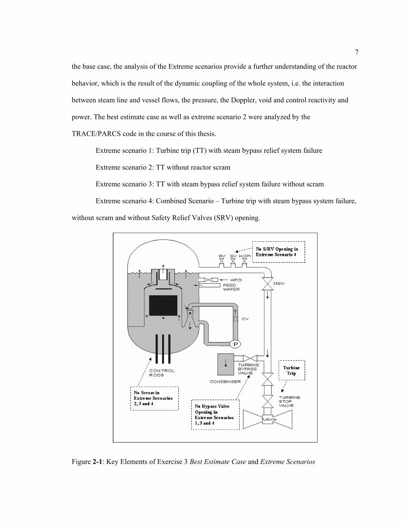
Figure 2-1: Key Elements of Exercise 3 Best Estimate Case and Extreme Scenarios.............7
Figure 2-2: Reactor Core Cross-sectional View ......................................................................12
Figure 2-3: PB2 Initial Fuel Assembly Lattice .......................................................................27
Figure 2-4: PB2 Reload Fuel Assembly Lattice for 100 mil Channels....................................28
Figure 2-5: PB2 Reload Fuel Assembly Lattice for 120 mil Channels....................................29
Figure 2-6: PB2 Reload Fuel Assembly Lattice for LTA Assemblies.....................................30
Figure 2-7: PSU Control Rod Grouping ..................................................................................31
Figure 2-8: Radial Distribution of Assembly Types................................................................32
Figure 2-9: Core Orificing and TIP System Arrangement.......................................................33
Figure 2-11: Elevation of Core Components ...........................................................................34
Figure 2-13: PB2 HP Control Rod Pattern...............................................................................38
Figure 2-14: PB2 TT2 Initial Core Axial Relative Power From P1 Edit.................................39
Figure 2-15: PB2 TT1 Initial Core Axial Relative Power From P1 Edit.................................44
Figure 2-16: PB2 TT3 Initial Core Axial Relative Power From P1 Edit.................................44
Figure 2-17: PB2 TT1 HP Control Rod Pattern.......................................................................45
Figure 2-18: PB2 TT3 HP Control Rod Pattern.......................................................................45
Figure 2-19: PB2 Power-flow Diagram...................................................................................48
Figure 2-20: PB2 EOC 2 Tests - Operational Time Line........................................................49
Figure 2-21: PB2 EOC 2 PT1 Test – Control Rod Pattern ......................................................51
Figure 2-22: PB2 EOC 2 PT1 Test - Average Axial Power Distribution ...............................52
Figure 2-23: PB2 EOC 2 PT2 Test – Control Rod Pattern ......................................................52
viii
Figure 2-24: PB2 EOC 2 PT2 Test - Average Axial Power Distribution ................................53
Figure 2-25: PB2 EOC 2 PT3 Test – Control Rod Pattern ......................................................53
Figure 2-26: PB2 EOC 2 PT3 Test - Average Axial Power Distribution ................................54
Figure 2-27: PB2 EOC 2 PT4 Test – Control Rod Pattern ......................................................54
Figure 2-28: PB2 EOC 2 PT4 Test - Average Axial Power Distribution ................................55
Figure 4-1: PB2 Input-data File Nodalization Scheme............................................................81
Figure 4-2: Thermal Hydraulic Channel Mapping for PB2 TT2 .............................................83
Figure 4-3: Steady State Core Average Void Fraction Distribution ........................................85
Figure 4-4: Steady State Coupled TRACE/PARCS Core Average Void Fraction Distribution ......................................................................................................................87
Figure 4-5: Steady State Coupled TRACE/PARCS Axial Power Profile................................87
Figure 4-6: Transient Stand Alone Steam Dome Pressure......................................................90
Figure 4-7: TRACE/PARCS Core Average Void Fraction .....................................................92
Figure 4-8: TRACE/PARCS Core Average Axial Power .......................................................92
Figure 4-9: TRACE/PARCS Component of Core Reactivity..................................................93
Figure 4-10: Transient Power with SCRAM ...........................................................................93
Figure 5-1: PT 1 Steady State TRACE/PARCS Axial Power Profile .....................................95
Figure 5-2: PT 2 Steady State TRACE/PARCS Axial Power Profile .....................................96
Figure 5-3: PT 3 Steady State TRACE/PARCS Axial Power Profile .....................................97
Figure 5-4: PT1 Control Rod Perturbation Power Response ...................................................99
Figure 5-5: PT2 Control Rod Perturbation Power Response ...................................................99
Figure 5-6: PT3 Control Rod Perturbation Power Response ...................................................100
Figure 5-7: PT1 Pressure Perturbation Power Response .........................................................100
Figure 5-8: PT2 Pressure Perturbation Power Response .........................................................101
Figure 5-9: PT3 Pressure Perturbation Power Response .........................................................101
ix
LIST OF TABLES
Table 2-1: PB2 Fuel Assembly Data. ......................................................................................13
Table 2-2: Assembly Design 1.................................................................................................13
Table 2-3: Assembly Design 1.................................................................................................14
Table 2-4: Assembly Design 2.................................................................................................14
Table 2-5: Assembly Design 3.................................................................................................15
Table 2-6: Assembly Design 4.................................................................................................15
Table 2-7: Assembly Design 5.................................................................................................16
Table 2-8: Assembly Design 6.................................................................................................16
Table 2-9: Decay Constant and Fractions of Delayed neutrons...............................................17
Table 2-10: Heavy-element Decay Heat Constants .................................................................17
Table 2-11: Assembly Design for Type 1 Initial Fuel .............................................................17
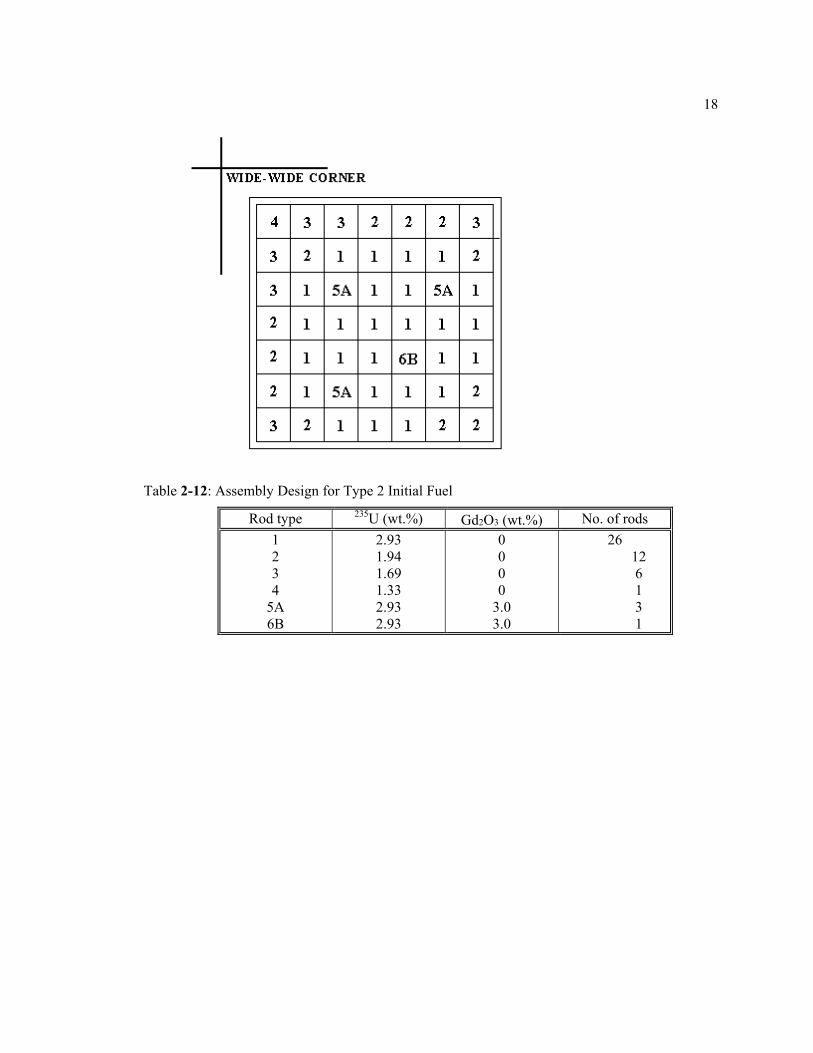
Table 2-12: Assembly Design for Type 2 Initial Fuel .............................................................18
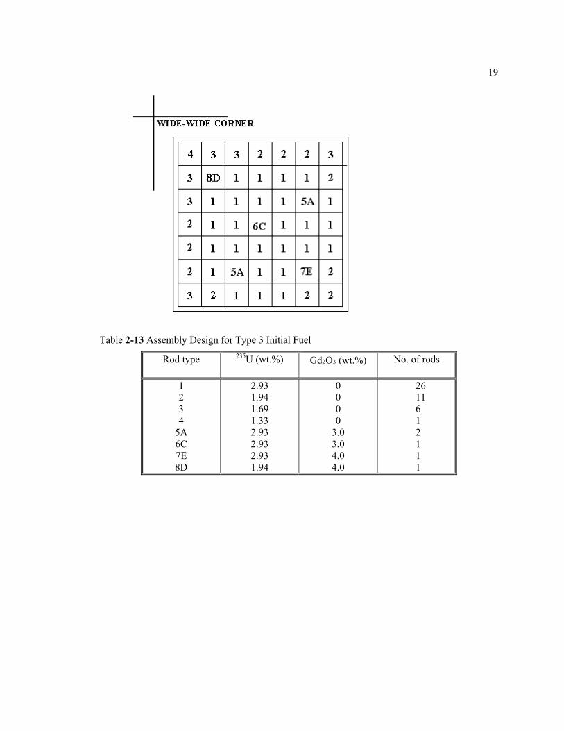
Table 2-13 Assembly Design for Type 3 Initial Fuel ..............................................................19
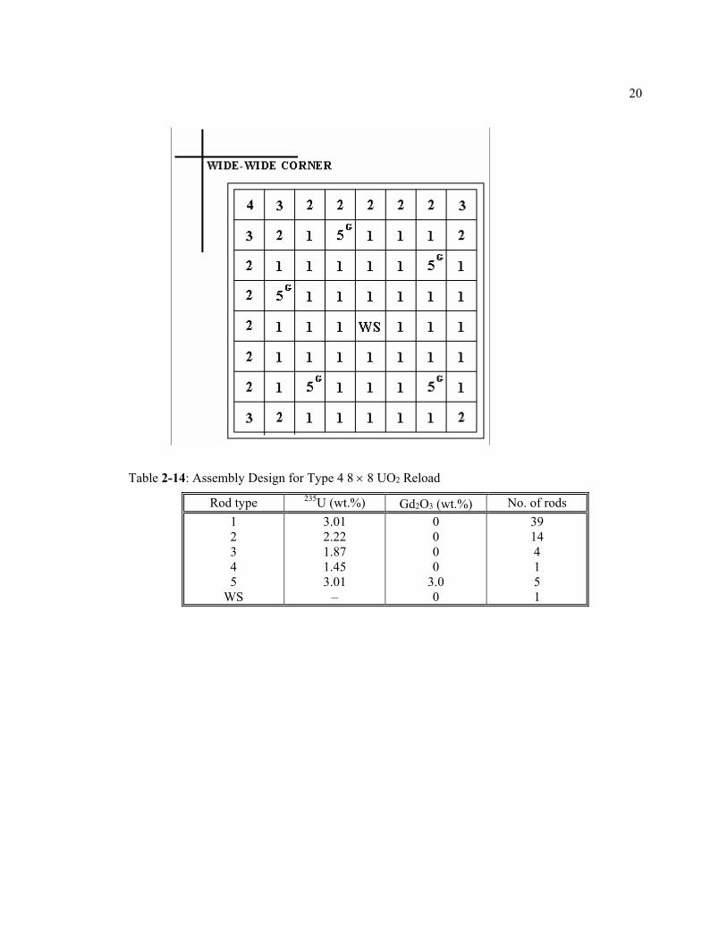
Table 2-14: Assembly Design for Type 4 8 × 8 UO2 Reload ..................................................20
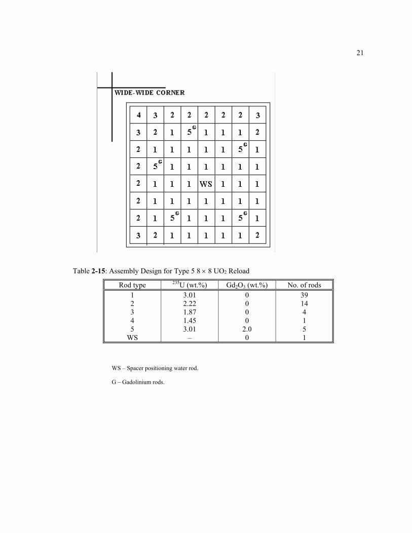
Table 2-15: Assembly Design for Type 5 8 × 8 UO2 Reload ..................................................21
Table 2-16: Assembly Design for Type 6 8 × 8 UO2 Reload, LTA.........................................22
Table 2-17: Control Rod Data (Movable Control Rods)..........................................................23
Table 2-18: Definition of Assembly Types..............................................................................23
Table 2-19: Composition Numbers in Axial Layer for Each Assembly Type.........................24
Table 2-20: Range of Variables ...............................................................................................25
Table 2-21: Key to Macroscopic Cross-section Tables ...........................................................26
x
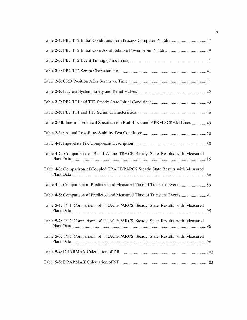
Table 2-1: PB2 TT2 Initial Conditions from Process Computer P1 Edit ................................37
Table 2-2: PB2 TT2 Initial Core Axial Relative Power From P1 Edit ....................................39
Table 2-3: PB2 TT2 Event Timing (Time in ms) ....................................................................41
Table 2-4: PB2 TT2 Scram Characteristics .............................................................................41
Table 2-5: CRD Position After Scram vs. Time ......................................................................41
Table 2-6: Nuclear System Safety and Relief Valves..............................................................42
Table 2-7: PB2 TT1 and TT3 Steady State Initial Conditions.................................................43
Table 2-8: PB2 TT1 and TT3 Scram Characteristics...............................................................46
Table 2-30: Interim Technical Specification Rod Block and APRM SCRAM Lines .............49
Table 2-31: Actual Low-Flow Stability Test Conditions.........................................................50
Table 4-1: Input-data File Component Description .................................................................80
Table 4-2: Comparison of Stand Alone TRACE Steady State Results with Measured Plant Data.........................................................................................................................85
Table 4-3: Comparison of Coupled TRACE/PARCS Steady State Results with Measured Plant Data.........................................................................................................................86
Table 4-4: Comparison of Predicted and Measured Time of Transient Events .......................89
Table 4-5: Comparison of Predicted and Measured Time of Transient Events .......................91
Table 5-1: PT1 Comparison of TRACE/PARCS Steady State Results with Measured Plant Data.........................................................................................................................95
Table 5-2: PT2 Comparison of TRACE/PARCS Steady State Results with Measured Plant Data.........................................................................................................................96
Table 5-3: PT3 Comparison of TRACE/PARCS Steady State Results with Measured Plant Data.........................................................................................................................96
Table 5-4: DRARMAX Calculation of DR .............................................................................102
Table 5-5: DRARMAX Calculation of NF..............................................................................102

xi
ACKNOWLEDGEMENTS
I would like to express my profound appreciation to a list of people who gave me support
and help for the completion of this work.
I thank my thesis advisor, Dr. Kostadin Ivanov for the guidance in my research and
accurate decisions concerning my academic requirements, in easy and troubled times. I would
like to thank, Dr. John Mahaffy for his scientific direction and guidance towards the application
TRACE thermal hydraulic code and his feedback prior the submission of the final thesis draft.
I thank Dr. Brenizer for spending time on reading my thesis.
I would like to thank Dr. Bedirhan Akdeniz who worked with me to obtain the results
presented in this dissertation, for his help and discussions concerning the Peach Bottom Turbine
Trip Benchmark and TRACE input deck.
Thanks to the late Dr. Tom Downar , Dr. Yunlin Xu for their guidance and discussions
during our weekly phone conferences on the subject.
I want to express my gratitude to the faculty and staff of the Mechanical and Nuclear
Engineering department.
Thanks to all the ones who believe in me in the adversity, my friends, my family and
wife who never doubted that I was able to reach the goal.
.
1
Chapter 1
Introduction
1 Background
The simulation of the nuclear reactor core behavior and plant dynamics as well as their
mutual interactions has a significant impact on the design and operation, safety and economics of
nuclear power plants. Three dimensional (3D) models of the reactor core incorporated into system
transient codes allows for a “best-estimate” calculation of interactions between the core behavior
and plant dynamics. Such models are used for simulating transients that involve core spatial
asymmetric phenomena and strong feedback effects between core neutronics and reactor thermal-
hydraulics.
The U. S. NRC uses computer models to study the phenomena associated with reactor
safety issues. The reactor system analysis code TRACE (TRAC RELAP5 Advanced
Computational Engine) is used to study the reactor coolant system under a wide variety of flow
conditions including multi-phase thermal hydraulics. Multidimensional time dependent power
distributions are required for accurate simulation and the PARCS (Purdue Advanced Reactor
Core Simulator) multi-dimensional reactor kinetics code has been coupled to TRACE to provide
accurate simulation capabilities of some reactor transient or accident scenarios. TRACE/PARCS
has been previously validated for Pressurized Water Reactor transient analysis using the
OECD/NEA Main Steam Line Break (MSLB) Benchmark [1].
The objectives of this thesis are focused on the assessment of TRACE/PARCS for BWR
transient analysis. In this case Boiling Water Reactor (BWR) Turbine Trip (TT) and Low Flow
Stability (LFS) tests are appropriate to assess the accuracy of TRACE/PARCS for BWR analysis.
2
Such tests exhibit significant space/time flux variations and utilize measurement of plant data
during the simulated transients. The selected experiments are the Peach Bottom 2 (PB2) TT and
LFS tests performed in 1977 [2]. After the completion of the turbine trip tests, several stability
tests were performed at PB2 and all of the tests are documented in EPRI reports [2], [3].
The OECD/NRC BWR TT Benchmark is designed to provide a validation basis for the
new generation best estimate codes – coupled 3D kinetics system thermal-hydraulic codes, and is
based on the second of the PB2 TT tests [4]. The codes were tested for simulation of the PB2 (a
General Electric designed BWR/4) TT transient with a sudden closure of the turbine stop valve.
Three turbine trip transients at different power levels were performed at the PB2 Nuclear
Power Plant (NPP) prior to shutdown for refuelling at the end of Cycle 2 in April 1977 [5, 6]. The
second test (TT2) was selected for the benchmark problem to investigate the effect of the
pressurisation transient (following the sudden closure of the turbine stop valve) on the neutron
flux in the reactor core. In a best-estimate manner the test conditions approached the design basis
conditions as closely as possible.
The transient selected for this benchmark is a dynamically complex event and it
constitutes a good problem to test the coupled codes on both levels: neutronics/thermal-hydraulics
coupling, and core/plant system coupling. In the TT2 test, the thermal-hydraulic feedback alone
limited the power peak and initiated the power reduction. The void feedback plays the major role
while the Doppler feedback plays a subordinate role. The reactor scram then inserted additional
negative reactivity and completed the power reduction and eventual core shutdown.
Three exercises were performed in the BWR TT Benchmark. These exercises include the
evaluation of different steady-states, and simulation of different transient scenarios.
The purpose of the first exercise is to test the thermal-hydraulic system response and to
initialize the participants’ system models for use of the second and third exercises on coupled 3-D
kinetics/system thermal-hydraulics simulations.
3
The second exercise consists of performing coupled-core boundary conditions
calculations. The purpose of the second exercise is to test and initiate the participants’ core
models. The thermal-hydraulic core boundary conditions provided are the core inlet pressure,
core exit pressure, core inlet temperature and core inlet flow.
The last exercise, Exercise 3, primarily comprises the best estimate of coupled 3D
core/thermal-hydraulic system modeling. This exercise combines elements of the first two
exercises of this benchmark and is an analysis of the transient in its entirety.
1.1 Peach Bottom Turbine Trip Tests
Both the Peach Bottom turbine trip transient and stability tests were performed at the End
of Cycle (EOC) 2. The Peach Bottom turbine trip experiments were pressurization events in
which the coupling between core phenomena and system dynamics plays an important role in
predicting the plant response.
The PB2 TT tests start with a sudden closure of the turbine stop valve (TSV) and then the
turbine by-pass valve begins to open. From a fluid phenomena point of view, pressure and flow
waves play an important role during the early phase of the transient (of about 1.5 seconds)
because rapid valve actions cause sonic waves, which propagate through the main steam piping to
the reactor core with relatively little attenuation. The induced core pressure oscillations results in
changes of the core void distribution and fluid flow. The magnitude of the neutron flux transient
taking place in the BWR core is affected by the initial rate of pressure rise caused by the pressure
oscillation and has a spatial variation. The simulation of the power response to the pressure pulse
and subsequent void collapse requires a 3D core modeling supplemented by 1D simulation of the
remainder of the reactor coolant system.
4
There have been several previous efforts to perform analysis of the OECD/NRC BWR
TT benchmark Peach Bottom turbine trip transients to include an analysis with the TRAC-
M/PARCS coupled code [7]. This previous effort with TRAC-M differs from the work here since
it used a TRAC-B model of Peach Bottom and specially modified version of the TRAC-M
computer code. For the current thesis, a Peach Bottom model was developed using TRACE
components and the information provided by the OECD/NRC BWR TT benchmark specification
[17]. Subsequently the TT and LFS test simulations were performed with a standard version of
the TRACE code v5.0rc3. The details of the TRACE Peach Bottom model and the steady state
and transient results are provided in Chapter 4. The work described in this thesis provides
modeling and results not only for TT2 test (within the framework of the OECD/NRC BWR TT
benchmark) but also for TT1, TT2 and four LFS tests.
1.2 Peach Bottom Low Flow Stability Tests
The Low Flow Stability Tests were intended to measure the reactor core stability margins
at the limiting conditions used in design and safety analysis, providing a one-to-one comparison
to design calculations. These tests were performed in the right boundary of the instability region
in the Power/Flow Map, i.e. in the area of low flow from 38 % to 51.3 % of total nominal core
flow rate and corresponding power of 43.5% to 60.6% of rated power
The stability tests were initiated from steady-state conditions after obtaining P1 edits
from the process computer for nuclear and thermal-hydraulic conditions of the core. The Peach
Bottom stability tests were conducted along the low-flow end of the rated power-flow line, and
along the power-flow line corresponding to minimum recirculation pump speed. The reactor core
stability margin was determined from an empirical model fitted to the experimentally derived
transfer function measurement between core pressure and the APRM, average neutron flux

5
signals. The low flow stability tests consisted of periodic pressure step recording and
pseudorandom pressure step recording.
Chapter 2 of this thesis gives detailed description about the PB2 TT tests and
OECD/NRC BWR TT benchmark as well as the LFS tests.
Chapter 3 describes the TRACE/PARCS codes and coupling methodology.
Chapter 4 provides comparative analysis of the TRACE/PARCS PB2 TT tests results
Chapter 5 provides comparative analysis of the TRACE/PARCS PB2 LFS tests results.
Chapter 6 provides a summary of the conclusions drawn from the analysis of
TRACE/PARCS.
6
Chapter 2
PB TT2 Benchmark and Low Flow Stability Tests Description
2.1 OECD/NRC BWR TT Benchmark Description
A TT transient in a BWR type reactor is considered one of the most complex events to be
analyzed because it involves the reactor core, the high pressure coolant boundary, associated
valves and piping in highly complex interactions with variables changing very rapidly. The
reference design for the BWR is derived from real reactor, plant and operation data for the PB2
NPP and it is based on the information provided in EPRI reports [2 - 5] and some additional
sources such as the PECo Energy Topical report [7].
The OECD/NRC BWR TT benchmark consists of three exercises. Exercise 1 and
Exercise 2 provided with the opportunity to initialize system and core models and to test code
capabilities for coupling of thermal hydraulic and neutronics phenomena. Measured core power
has been used as a boundary condition in the first exercise, and only core calculations have been
performed using specified boundary conditions in the second exercise. The successes of Exercise
1 and 2 lead to the third exercise which combines elements of the first two exercises of this
benchmark and is an analysis of the transient and its entirety.
Exercise 3 is composed of base case (so-called Best Estimate Case) and hypothetical
cases (so-called Extreme Scenarios) The purpose of the Exercise 3 Best Estimate Case is to
provide comprehensive assessment of the code in analyzing complex transients with 3D coupled
core and system calculations. In order to validate such assessments, available measured plant data
are utilized for this case during the comparative analyses presented in this thesis. In addition to
7
the base case, the analysis of the Extreme scenarios provide a further understanding of the reactor
behavior, which is the result of the dynamic coupling of the whole system, i.e. the interaction
between steam line and vessel flows, the pressure, the Doppler, void and control reactivity and
power. The best estimate case as well as extreme scenario 2 were analyzed by the
TRACE/PARCS code in the course of this thesis.
Extreme scenario 1: Turbine trip (TT) with steam bypass relief system failure
Extreme scenario 2: TT without reactor scram
Extreme scenario 3: TT with steam bypass relief system failure without scram
Extreme scenario 4: Combined Scenario – Turbine trip with steam bypass system failure,
without scram and without Safety Relief Valves (SRV) opening.
Figure 2-1: Key Elements of Exercise 3 Best Estimate Case and Extreme Scenarios
8
The key elements of Exercise 3 are illustrated in the simple BWR schematic given above.
Extreme Scenario 2 (TT without scram) can be considered as single failure and therefore provides
information from the perspective of the safety of the plant. Extreme Scenario 3 (combination of 1
and 2) considers the coincidence of two independent failures. Extreme Scenario 4 (in addition to
3 no opening of safety relief valves) considers the coincidence of three independent failures,
which are extremely unlikely from a safety perspective and therefore not considered in the current
work. In the base case, SRVs are not opening during the transient while this happens in the
extreme scenario 2. In the hypothetical case, the dynamical response of the system due to the
interaction of the flow in the steam line with the dynamics of the SRVs happens to be more
challenging for the coupled codes. It should be noted that no comparison with measured data is
possible for the extreme cases since they are hypothetical scenarios. Therefore, submitted extreme
scenario results are compared with an “average” of the results of the OECD/NRC BWR TT
benchmark participants.
The PB2 neutronics and thermal-hydraulic data as well as initial TT2 conditions for
steady state and transient calculations are given in the following subsections of this chapter.
2.1.1 Core and Neutronics Data
The reference design for the BWR is derived from real reactor, plant and operation data
for the PB2 BWR/4 NPP and it is based on the information provided in EPRI reports and some
additional sources such as the PECO Energy Topical Report. This section specifies the core and
neutronics data to be used in the calculation of Exercise 3
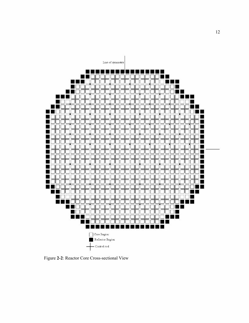
The radial geometry of the reactor core is shown in Figure 2-2. At radial plane the core is
divided into cells 15.24 cm wide, each corresponding to one fuel assembly (FA), plus a radial
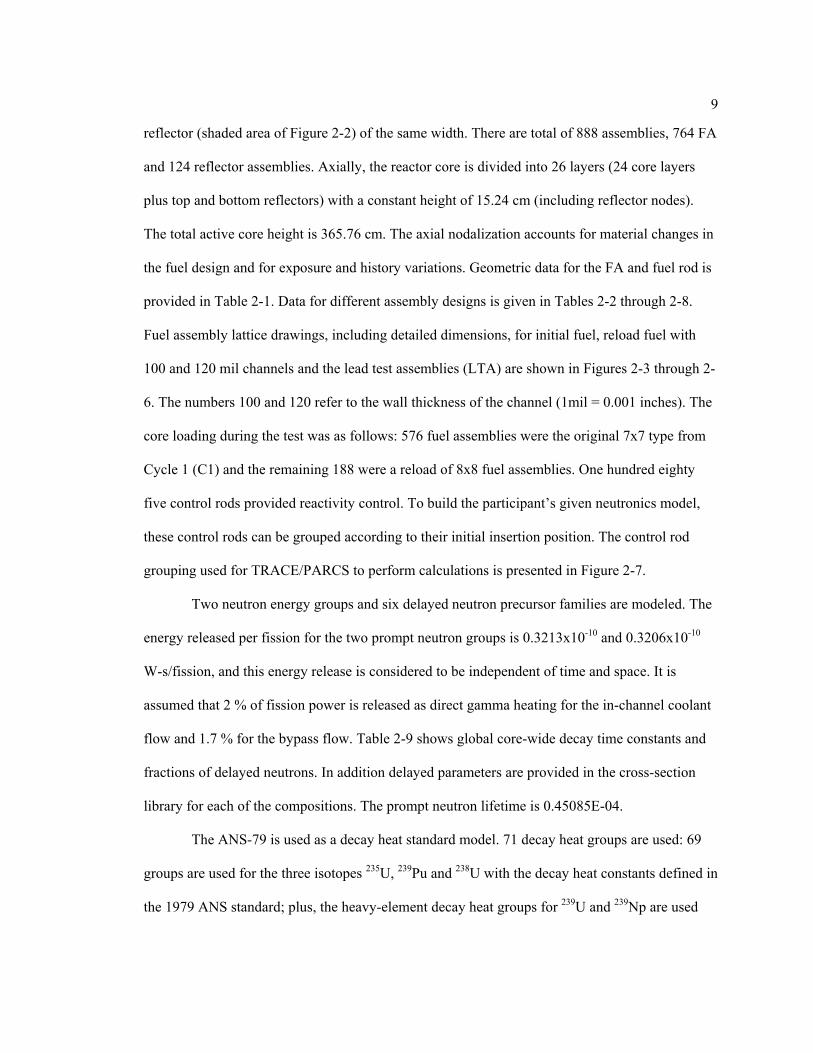
9
reflector (shaded area of Figure 2-2) of the same width. There are total of 888 assemblies, 764 FA
and 124 reflector assemblies. Axially, the reactor core is divided into 26 layers (24 core layers
plus top and bottom reflectors) with a constant height of 15.24 cm (including reflector nodes).
The total active core height is 365.76 cm. The axial nodalization accounts for material changes in
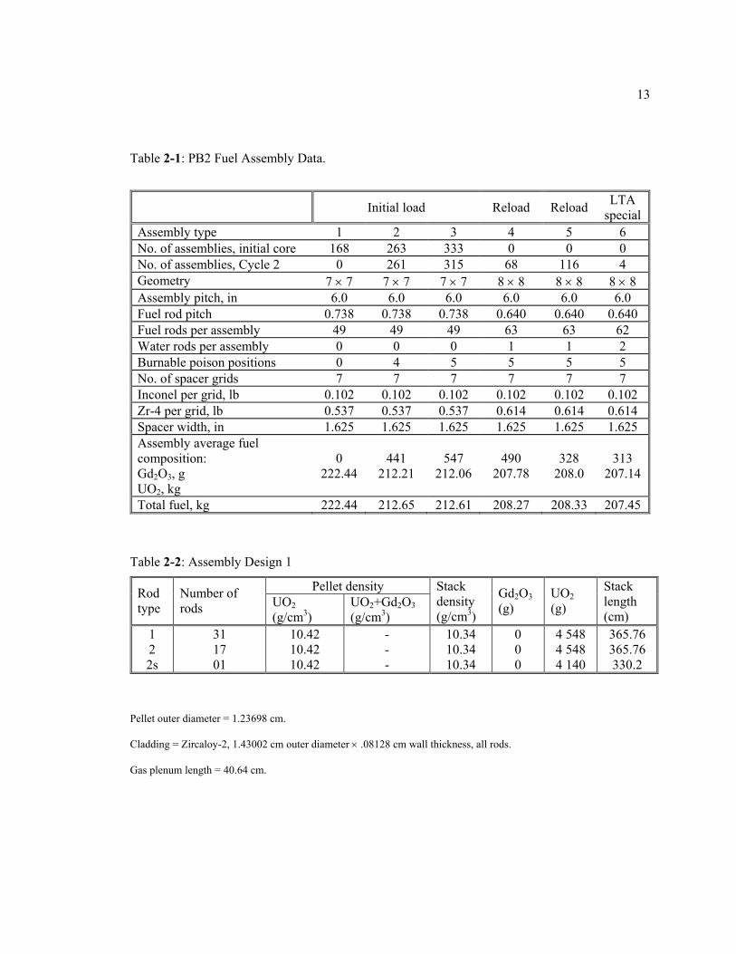
the fuel design and for exposure and history variations. Geometric data for the FA and fuel rod is
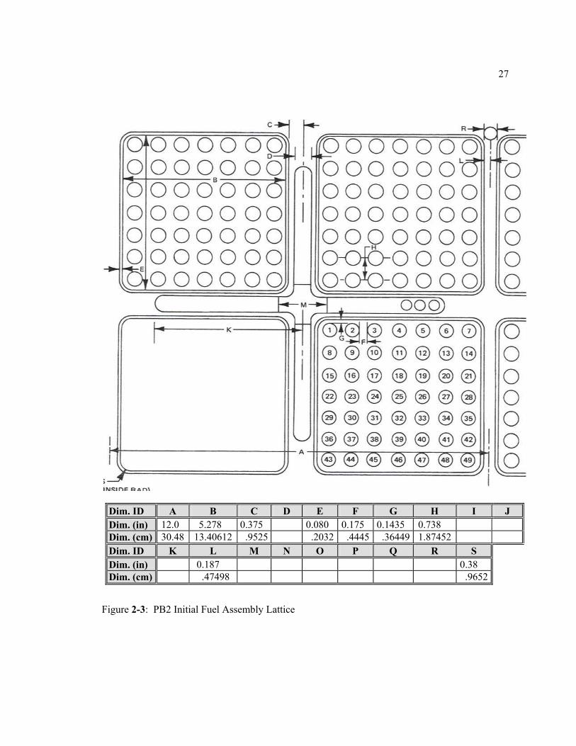
provided in Table 2-1. Data for different assembly designs is given in Tables 2-2 through 2-8.
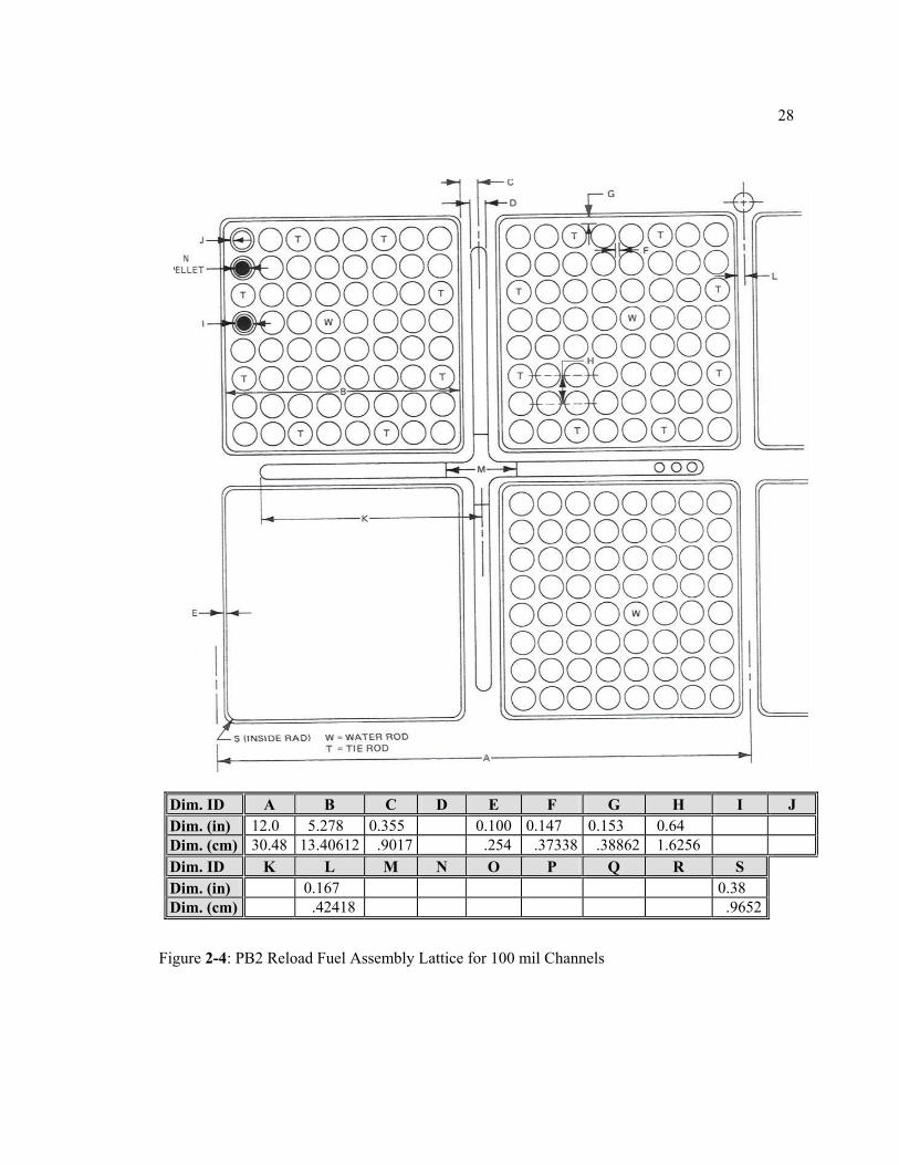
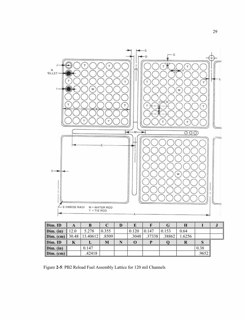
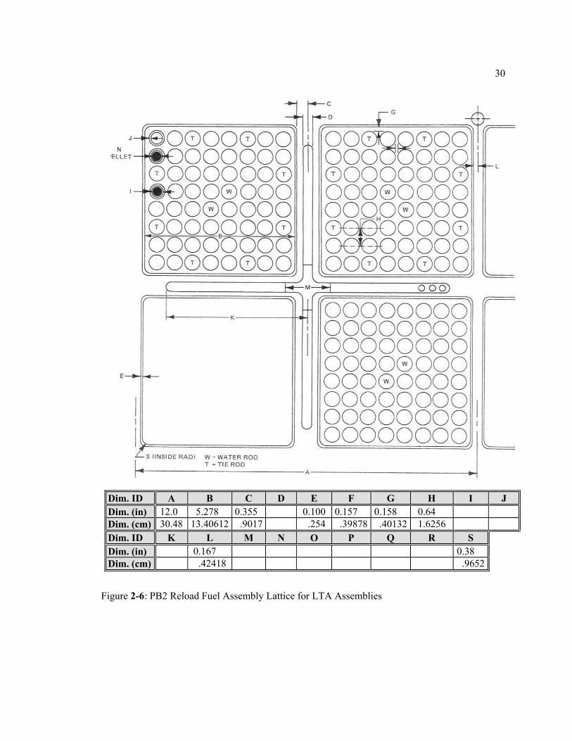
Fuel assembly lattice drawings, including detailed dimensions, for initial fuel, reload fuel with
100 and 120 mil channels and the lead test assemblies (LTA) are shown in Figures 2-3 through 2-
6. The numbers 100 and 120 refer to the wall thickness of the channel (1mil = 0.001 inches). The
core loading during the test was as follows: 576 fuel assemblies were the original 7x7 type from
Cycle 1 (C1) and the remaining 188 were a reload of 8x8 fuel assemblies. One hundred eighty
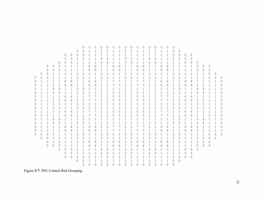
five control rods provided reactivity control. To build the participant’s given neutronics model,
these control rods can be grouped according to their initial insertion position. The control rod
grouping used for TRACE/PARCS to perform calculations is presented in Figure 2-7.
Two neutron energy groups and six delayed neutron precursor families are modeled. The
energy released per fission for the two prompt neutron groups is 0.3213x10⁻¹⁰ and 0.3206x10⁻¹⁰
W-s/fission, and this energy release is considered to be independent of time and space. It is
assumed that 2 % of fission power is released as direct gamma heating for the in-channel coolant
flow and 1.7 % for the bypass flow. Table 2-9 shows global core-wide decay time constants and
fractions of delayed neutrons. In addition delayed parameters are provided in the cross-section
library for each of the compositions. The prompt neutron lifetime is 0.45085E-04.
The ANS-79 is used as a decay heat standard model. 71 decay heat groups are used: 69
groups are used for the three isotopes 235U, 239Pu and 238U with the decay heat constants defined in
the 1979 ANS standard; plus, the heavy-element decay heat groups for 239U and 239Np are used

10
with constants given in Table 2-10. The assumption of an infinite operation at a power of 3 293
MWt is used.
Nineteen assembly types are contained within the core geometry with 435 compositions.
The corresponding sets of cross-sections are provided. Each composition is defined by material
properties (due to changes in the fuel design) and burn-up. The burn-up dependence is a three-
component vector of variables: exposure (GWd/t), spectral history (void fraction) and control rod
history. Assembly designs are defined in Tables 2-11 through 2-15. Control rod geometry data is
provided in Table 2-16. The definition of assembly type is shown in Table 2-17. The radial
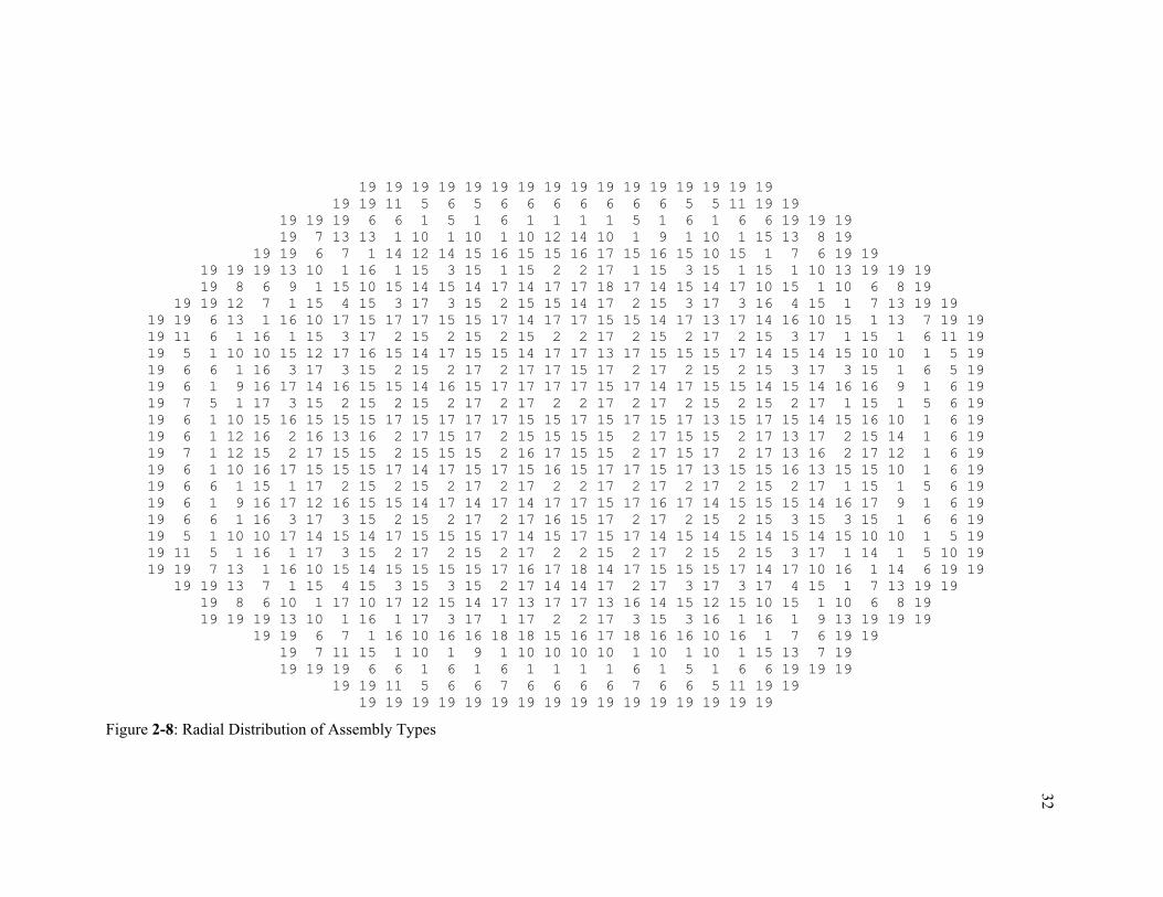
distribution of these assembly types within the reactor geometry is shown in Figure 2-8. The axial
locations of compositions of each assembly type are shown in Table 2-18.
A complete set of diffusion coefficients, macroscopic cross-sections for scattering,
absorption, and fission, assembly discontinuity factors (ADFs), as a function of the moderator
density and fuel temperature is defined for each composition. The group inverse neutron
velocities are also provided for each composition. Dependence of the cross-sections of the above
variables is specified through a two-dimensional table lookup. Each composition is assigned to a
cross-section set containing separate tables for the diffusion coefficients and cross-sections, with
each point in the table representing a possible core state. The expected range of the transient is
covered by the selection of an adequate range for the independent variables shown in Table 2-19.
Specifically, Exercise 1 was used for selecting the range of thermal-hydraulic variables. A steady
state calculation was run using the TRAC-BF1 code and initial conditions of the second turbine
trip for choosing discrete values of the thermal hydraulic variables (pressure, void fraction and
coolant/moderator temperature). A transient calculation was performed to determine the expected
range of change of the above variables.
A modified linear interpolation scheme (which includes extrapolation outside the
thermal-hydraulic range) is used to obtain the appropriate total cross-sections from the tabulated
11
ones based on the reactor conditions being modeled. Table 2-20 shows the definition of a cross-
section table associated with a composition. Table 2-21 shows the macroscopic cross-section
table structure for one cross-section set. All cross section sets are assembled into a cross-section
library. The cross-sections are provided in a separate libraries for rodded (nemtabr) and un-
rodded compositions (nemtab).
Lattice physics calculations are performed by homogenizing the fuel lattice and the
bypass flow associated with it. When obtaining the average coolant density, a correction that
accounts for the bypass channel conditions should be included since this is going to influence the
feedback effect on the cross-section calculation through the average coolant density. The
following approach should be applied:
( )act
satbypbypactacteffact A
AA ρρρρ
−+= 2.1
where effactρ is the effective average coolant density for cross-section calculation, bypρ
is the average moderator coolant density of the bypass channel, satρ is the saturated moderator
coolant density of the bypass channel, actA is flow cross-sectional area of the active heated
channel and bypA is the flow cross-sectional area of the bypass channel.
Bypass conditions should be obtained by adding a bypass channel to represent the core
bypass region in the thermal-hydraulic model
12
Figure 2-2: Reactor Core Cross-sectional View
13
Initial load Reload Reload LTA special
Assembly type 1 2 3 4 5 6 No. of assemblies, initial core 168 263 333 0 0 0 No. of assemblies, Cycle 2 0 261 315 68 116 4 Geometry 7 × 7 7 × 7 7 × 7 8 × 8 8 × 8 8 × 8 Assembly pitch, in 6.0 6.0 6.0 6.0 6.0 6.0 Fuel rod pitch 0.738 0.738 0.738 0.640 0.640 0.640 Fuel rods per assembly 49 49 49 63 63 62 Water rods per assembly 0 0 0 1 1 2 Burnable poison positions 0 4 5 5 5 5 No. of spacer grids 7 7 7 7 7 7 Inconel per grid, lb 0.102 0.102 0.102 0.102 0.102 0.102 Zr-4 per grid, lb 0.537 0.537 0.537 0.614 0.614 0.614 Spacer width, in 1.625 1.625 1.625 1.625 1.625 1.625 Assembly average fuel composition: Gd2O3, g UO2, kg
0
222.44
441
212.21
547
212.06
490
207.78
328
208.0
313
207.14
Total fuel, kg 222.44 212.65 212.61 208.27 208.33 207.45
Pellet outer diameter = 1.23698 cm.
Cladding = Zircaloy-2, 1.43002 cm outer diameter × .08128 cm wall thickness, all rods.
Gas plenum length = 40.64 cm.
Table 2-1: PB2 Fuel Assembly Data.
Table 2-2: Assembly Design 1
Pellet density Rod type
Number of rods UO2
(g/cm3) UO2+Gd2O3 (g/cm3)
Stack density (g/cm3)
Gd2O3 (g)
UO2 (g)
Stack length (cm)
1 2 2s
31 17 01
10.42 10.42 10.42
- - -
10.34 10.34 10.34
0 0 0
4 548 4 548 4 140
365.76 365.76 330.2
14
Pellet outer diameter = 1.23698 cm.
Cladding = Zircaloy-2, 1.43002 cm outer diameter × .08128 cm wall thickness, all rods.
Gas plenum length = 40.64 cm.
Pellet outer diameter = 1.21158 cm.
Cladding = Zircaloy-2, 1.43002 cm outer diameter × .09398 cm wall thickness, all rods.
Gas plenum length = 40.132 cm.
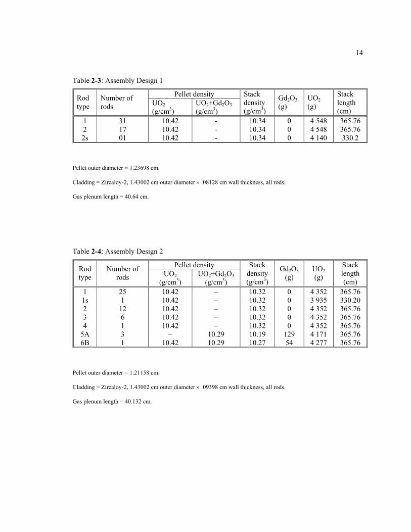
Table 2-3: Assembly Design 1
Pellet density Rod type
Number of rods UO2
(g/cm3) UO2+Gd2O3 (g/cm3)
Stack density (g/cm3)
Gd2O3 (g)
UO2 (g)
Stack length (cm)
1 2 2s
31 17 01
10.42 10.42 10.42
- - -
10.34 10.34 10.34
0 0 0
4 548 4 548 4 140
365.76 365.76 330.2
Table 2-4: Assembly Design 2
Pellet density Rod type
Number of rods UO2
(g/cm3) UO2+Gd2O3
(g/cm3)
Stack density (g/cm3)
Gd2O3 (g)
UO2 (g)
Stack length (cm)
1 1s 2 3 4
5A 6B
25 1
12 6 1 3 1
10.42 10.42 10.42 10.42 10.42
– 10.42
– – – – –
10.29 10.29
10.32 10.32 10.32 10.32 10.32 10.19 10.27
0 0 0 0 0
129 54
4 352 3 935 4 352 4 352 4 352 4 171 4 277
365.76 330.20 365.76 365.76 365.76 365.76 365.76
15
Pellet outer diameter = 1.21158 cm.
Cladding = Zircaloy-2, 1.43002 cm outer diameter × .09398 cm wall thickness, all rods.
Gas plenum length = 40.132 cm.
Pellet outer diameter = 1.05664 cm.
Cladding = Zircaloy-2, 1.25222 cm outer diameter × .08636 cm wall thickness, all rods.
Gas plenum length = 40.64 cm except water rod.
Gd2O3 in rod type 5 runs full 365.76 cm.
Water rod (WS) has holes drilled top and bottom to provide water flow and little or no boiling.
Water rod is also a spacer positioning rod.
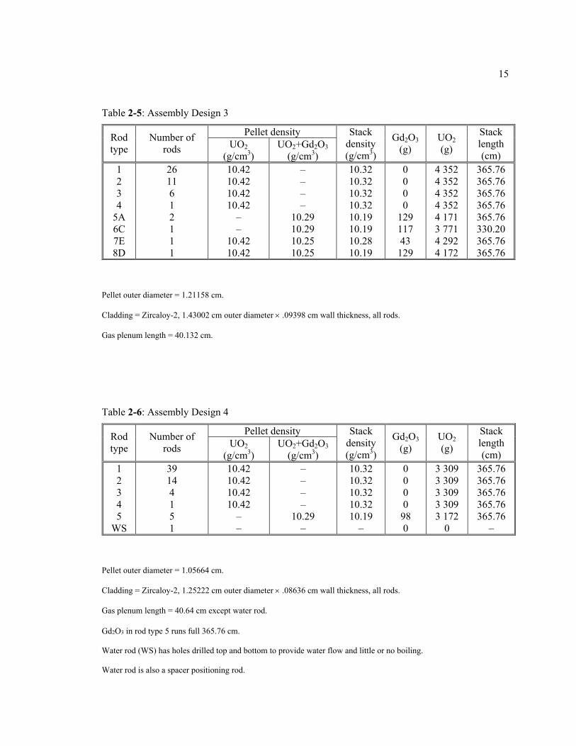
Table 2-5: Assembly Design 3
Pellet density Rod type
Number of rods UO2
(g/cm3) UO2+Gd2O3
(g/cm3)
Stack density (g/cm3)
Gd2O3 (g)
UO2 (g)
Stack length (cm)
1 2 3 4
5A 6C 7E 8D
26 11 6 1 2 1 1 1
10.42 10.42 10.42 10.42
– –
10.42 10.42
– – – –
10.29 10.29 10.25 10.25
10.32 10.32 10.32 10.32 10.19 10.19 10.28 10.19
0 0 0 0
129 117 43
129
4 352 4 352 4 352 4 352 4 171 3 771 4 292 4 172
365.76 365.76 365.76 365.76 365.76 330.20 365.76 365.76
Table 2-6: Assembly Design 4
Pellet density Rod type
Number of rods UO2
(g/cm3) UO2+Gd2O3
(g/cm3)
Stack density (g/cm3)
Gd2O3 (g)
UO2 (g)
Stack length (cm)
1 2 3 4 5
WS
39 14 4 1 5 1
10.42 10.42 10.42 10.42
– –
– – – –
10.29 –
10.32 10.32 10.32 10.32 10.19
–
0 0 0 0
98 0
3 309 3 309 3 309 3 309 3 172
0
365.76 365.76 365.76 365.76 365.76
–
16
Pellet outer diameter = 1.05664 cm.
Cladding = Zircaloy-2, 1.25222 cm outer diameter × .08636 cm wall thickness, all rods.
Gas plenum length = 40.64 cm, except water rod.
Gd2O3 in rod type 5 runs full 365.76 cm.
Water rod (WS) has holes drilled top and bottom to provide water flow and little or no boiling.
Water rod is also a spacer positioning rod.
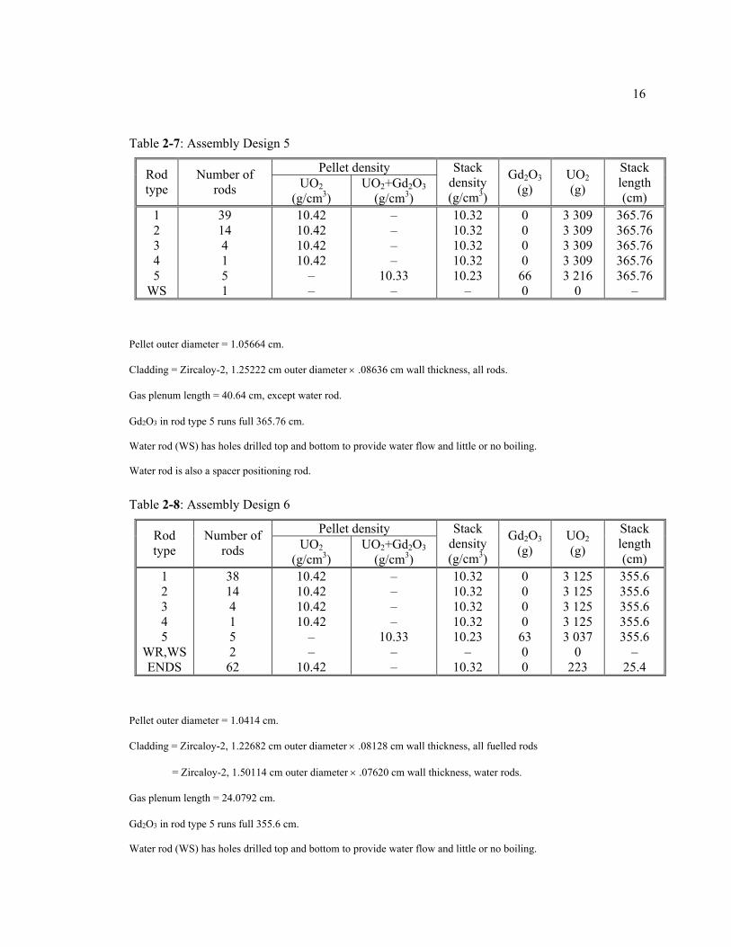
Pellet outer diameter = 1.0414 cm.
Cladding = Zircaloy-2, 1.22682 cm outer diameter × .08128 cm wall thickness, all fuelled rods
= Zircaloy-2, 1.50114 cm outer diameter × .07620 cm wall thickness, water rods.
Gas plenum length = 24.0792 cm.
Gd2O3 in rod type 5 runs full 355.6 cm.
Water rod (WS) has holes drilled top and bottom to provide water flow and little or no boiling.
Table 2-7: Assembly Design 5
Pellet density Rod type
Number of rods UO2
(g/cm3) UO2+Gd2O3
(g/cm3)
Stack density (g/cm3)
Gd2O3 (g)
UO2 (g)
Stack length (cm)
1 2 3 4 5
WS
39 14 4 1 5 1
10.42 10.42 10.42 10.42
– –
– – – –
10.33 –
10.32 10.32 10.32 10.32 10.23
–
0 0 0 0
66 0
3 309 3 309 3 309 3 309 3 216
0
365.76 365.76 365.76 365.76 365.76
–
Table 2-8: Assembly Design 6
Pellet density Rod type
Number of rods UO2
(g/cm3) UO2+Gd2O3
(g/cm3)
Stack density (g/cm3)
Gd2O3 (g)
UO2 (g)
Stack length (cm)
1 2 3 4 5
WR,WS ENDS
38 14 4 1 5 2
62
10.42 10.42 10.42 10.42
– –
10.42
– – – –
10.33 – –
10.32 10.32 10.32 10.32 10.23
– 10.32
0 0 0 0
63 0 0
3 125 3 125 3 125 3 125 3 037
0 223
355.6 355.6 355.6 355.6 355.6
– 25.4
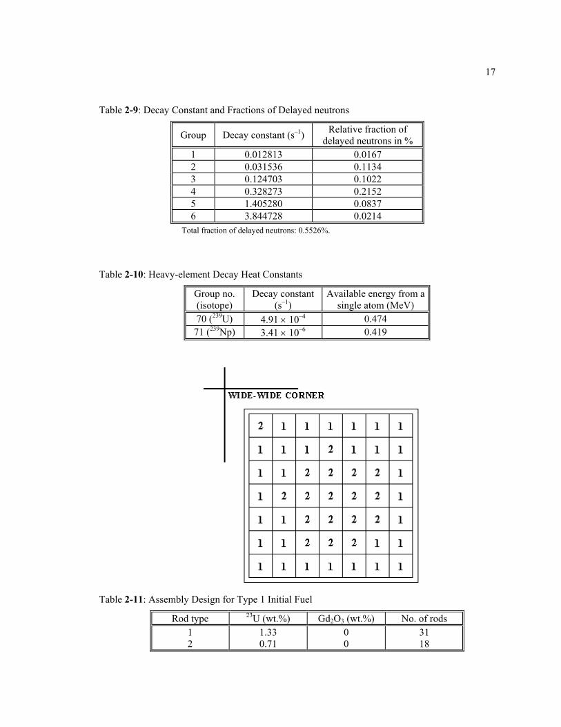
17
Table 2-9: Decay Constant and Fractions of Delayed neutrons
Group Decay constant (s–1) Relative fraction of delayed neutrons in %
1 0.012813 0.0167 2 0.031536 0.1134 3 0.124703 0.1022 4 0.328273 0.2152 5 1.405280 0.0837 6 3.844728 0.0214
Total fraction of delayed neutrons: 0.5526%.
Table 2-10: Heavy-element Decay Heat Constants
Group no. (isotope)
Decay constant(s–1)
Available energy from a single atom (MeV)
70 (239U) 4.91 × 10⁻⁴ 0.474 71 (239Np) 3.41 × 10⁻⁶ 0.419
Table 2-11: Assembly Design for Type 1 Initial Fuel
Rod type 23U (wt.%) Gd2O3 (wt.%) No. of rods 1 2
1.33 0.71
0 0
31 18
18
Table 2-12: Assembly Design for Type 2 Initial Fuel
Rod type 235U (wt.%) Gd2O3 (wt.%) No. of rods 1 2 3 4
5A 6B
2.93 1.94 1.69 1.33 2.93 2.93
0 0 0 0
3.0 3.0
26 12 6 1 3 1
19
Table 2-13 Assembly Design for Type 3 Initial Fuel
Rod type 235U (wt.%) Gd2O3 (wt.%) No. of rods
1 2 3 4
5A 6C 7E 8D
2.93 1.94 1.69 1.33 2.93 2.93 2.93 1.94
0 0 0 0
3.0 3.0 4.0 4.0
26 11 6 1 2 1 1 1
20
Table 2-14: Assembly Design for Type 4 8 × 8 UO2 Reload
Rod type 235U (wt.%) Gd2O3 (wt.%) No. of rods 1 2 3 4 5
WS
3.01 2.22 1.87 1.45 3.01
–
0 0 0 0
3.0 0
39 14 4 1 5 1
21
WS – Spacer positioning water rod.
G – Gadolinium rods.
Table 2-15: Assembly Design for Type 5 8 × 8 UO2 Reload
Rod type 235U (wt.%) Gd2O3 (wt.%) No. of rods 1 2 3 4 5
WS
3.01 2.22 1.87 1.45 3.01
–
0 0 0 0
2.0 0
39 14 4 1 5 1
22
WS – Spacer positioning water rod.
WR – Water rod.
G – Gadolinium rods.
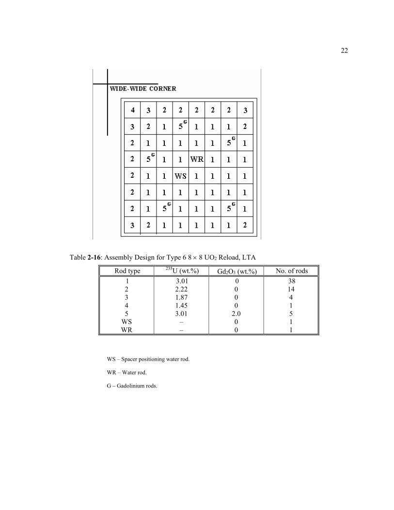
Table 2-16: Assembly Design for Type 6 8 × 8 UO2 Reload, LTA
Rod type 235U (wt.%) Gd2O3 (wt.%) No. of rods 1 2 3 4 5
WS WR
3.01 2.22 1.87 1.45 3.01
– –
0 0 0 0
2.0 0 0
38 14 4 1 5 1 1
23
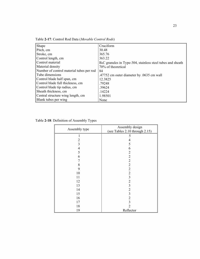
Table 2-17: Control Rod Data (Movable Control Rods)
Shape Pitch, cm Stroke, cm Control length, cm Control material Material density Number of control material tubes per rodTube dimensions Control blade half span, cm Control blade full thickness, cm Control blade tip radius, cm Sheath thickness, cm Central structure wing length, cm Blank tubes per wing
Cruciform 30.48 365.76 363.22 B4C granules in Type-304, stainless steel tubes and sheath 70% of theoretical 84 .47752 cm outer diameter by .0635 cm wall 12.3825 .79248 .39624 .14224 1.98501 None
Table 2-18: Definition of Assembly Types
Assembly type Assembly design (see Tables 2.10 through 2.15)
01 02 03 04 05 06 07 08 09 10 11 12 13 14 15 16 17 18 19
5 4 5 6 2 2 2 2 2 2 3 2 3 2 3 2 3 2
Reflector
24
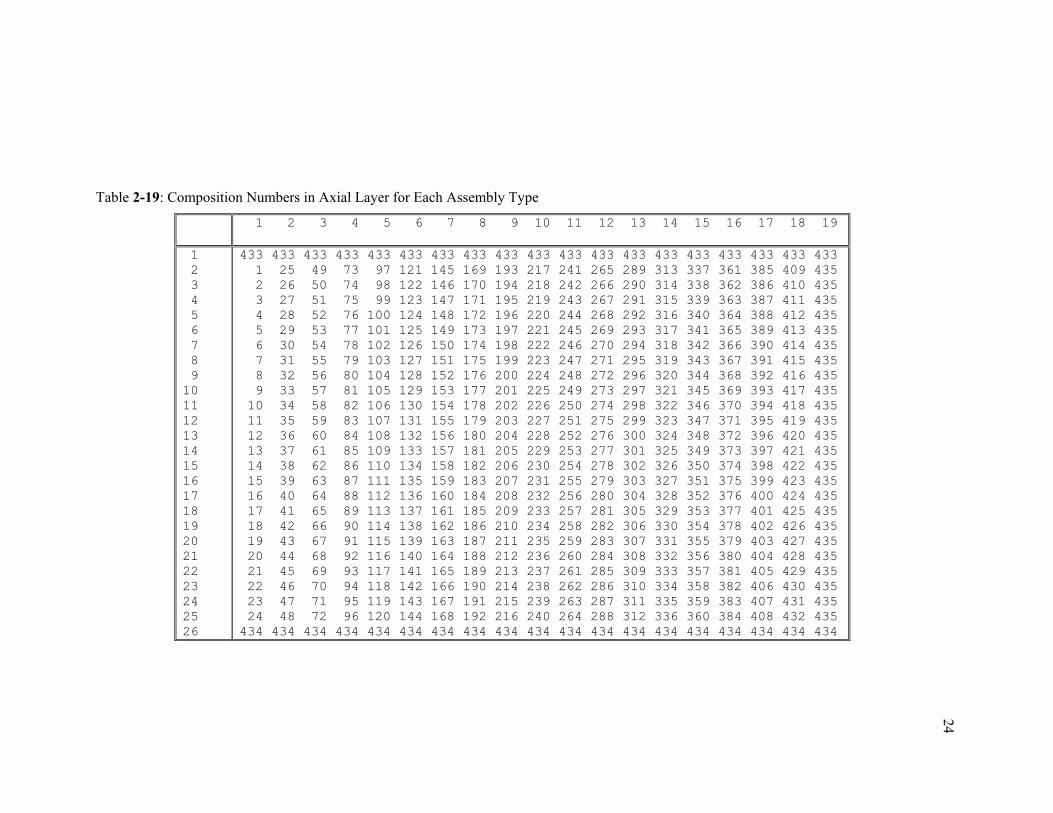
Table 2-19: Composition Numbers in Axial Layer for Each Assembly Type
1 2 3 4 5 6 7 8 9 10 11 12 13 14 15 16 17 18 19
1 2 3 4 5 6 7 8 9 10 11 12 13 14 15 16 17 18 19 20 21 22 23 24 25 26
433 433 433 433 433 433 433 433 433 433 433 433 433 433 433 433 433 433 433 1 25 49 73 97 121 145 169 193 217 241 265 289 313 337 361 385 409 435 2 26 50 74 98 122 146 170 194 218 242 266 290 314 338 362 386 410 435 3 27 51 75 99 123 147 171 195 219 243 267 291 315 339 363 387 411 435 4 28 52 76 100 124 148 172 196 220 244 268 292 316 340 364 388 412 435 5 29 53 77 101 125 149 173 197 221 245 269 293 317 341 365 389 413 435 6 30 54 78 102 126 150 174 198 222 246 270 294 318 342 366 390 414 435 7 31 55 79 103 127 151 175 199 223 247 271 295 319 343 367 391 415 435 8 32 56 80 104 128 152 176 200 224 248 272 296 320 344 368 392 416 435 9 33 57 81 105 129 153 177 201 225 249 273 297 321 345 369 393 417 435 10 34 58 82 106 130 154 178 202 226 250 274 298 322 346 370 394 418 435 11 35 59 83 107 131 155 179 203 227 251 275 299 323 347 371 395 419 435 12 36 60 84 108 132 156 180 204 228 252 276 300 324 348 372 396 420 435 13 37 61 85 109 133 157 181 205 229 253 277 301 325 349 373 397 421 435 14 38 62 86 110 134 158 182 206 230 254 278 302 326 350 374 398 422 435 15 39 63 87 111 135 159 183 207 231 255 279 303 327 351 375 399 423 435 16 40 64 88 112 136 160 184 208 232 256 280 304 328 352 376 400 424 435 17 41 65 89 113 137 161 185 209 233 257 281 305 329 353 377 401 425 435 18 42 66 90 114 138 162 186 210 234 258 282 306 330 354 378 402 426 435 19 43 67 91 115 139 163 187 211 235 259 283 307 331 355 379 403 427 435 20 44 68 92 116 140 164 188 212 236 260 284 308 332 356 380 404 428 435 21 45 69 93 117 141 165 189 213 237 261 285 309 333 357 381 405 429 435 22 46 70 94 118 142 166 190 214 238 262 286 310 334 358 382 406 430 435 23 47 71 95 119 143 167 191 215 239 263 287 311 335 359 383 407 431 435 24 48 72 96 120 144 168 192 216 240 264 288 312 336 360 384 408 432 435 434 434 434 434 434 434 434 434 434 434 434 434 434 434 434 434 434 434 434
25
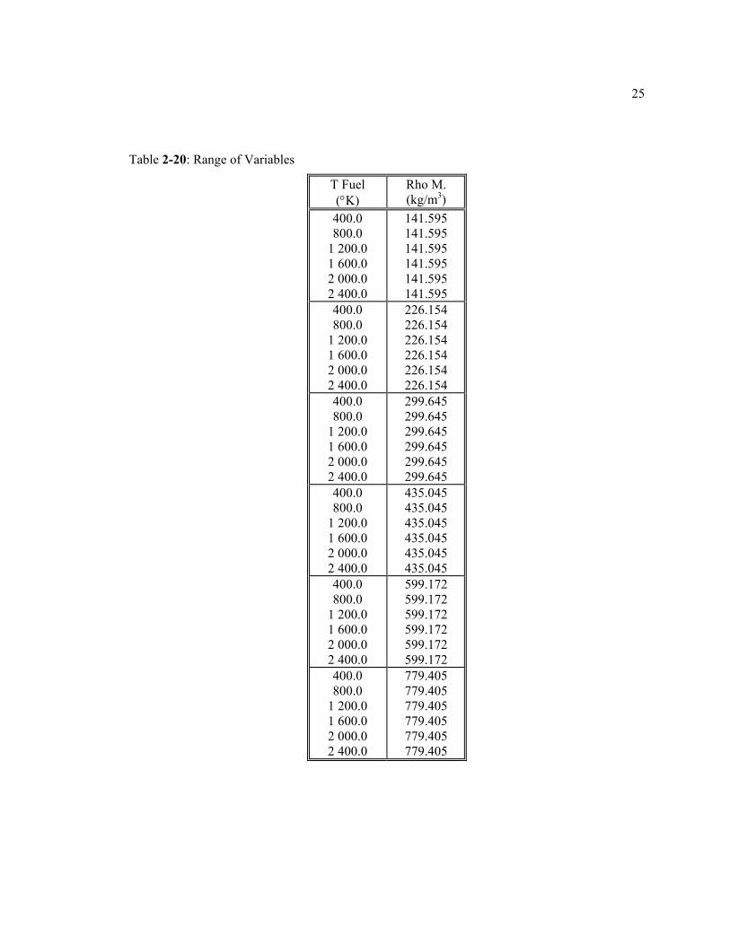
Table 2-20: Range of Variables
T Fuel (°K)
Rho M. (kg/m3)
400.0 800.0
1 200.0 1 600.0 2 000.0 2 400.0
141.595 141.595 141.595 141.595 141.595 141.595
400.0 800.0
1 200.0 1 600.0 2 000.0 2 400.0
226.154 226.154 226.154 226.154 226.154 226.154
400.0 800.0
1 200.0 1 600.0 2 000.0 2 400.0
299.645 299.645 299.645 299.645 299.645 299.645
400.0 800.0
1 200.0 1 600.0 2 000.0 2 400.0
435.045 435.045 435.045 435.045 435.045 435.045
400.0 800.0
1 200.0 1 600.0 2 000.0 2 400.0
599.172 599.172 599.172 599.172 599.172 599.172
400.0 800.0
1 200.0 1 600.0 2 000.0 2 400.0
779.405 779.405 779.405 779.405 779.405 779.405

26
Table 2-21: Key to Macroscopic Cross-section Tables
Tf1 Tf2 Tf3 Tf4 Tf5 Tf6 Where: ρm1 ρm2 ρm3 ρm4 ρm5 ρm6 – Tf is the Doppler (fuel) temperature (°K) Σ1 Σ2 ... – ρm is the moderator density (kg/m3) ... Σ34 Σ35 Σ36 Macroscopic cross-sections are in units of cm–1
27
Dim. ID A B C D E F G H I J Dim. (in) 12.00 c5.27800 0.3750 0.0800 0.1750 0.14350 0.73800 Dim. (cm) 30.48 13.40612 0.9525 0.2032 0.4445 0.36449 1.87452 Dim. ID K L M N O P Q R S Dim. (in) 0.18700 0.3800 Dim. (cm) 0.47498 0.9652
Figure 2-3: PB2 Initial Fuel Assembly Lattice
28
Dim. ID A B C D E F G H I J Dim. (in) 12.00 05.27800 0.3550 0.100 0.14700 0.15300 0.6400 Dim. (cm) 30.48 13.40612 0.9017 0.254 0.37338 0.38862 1.6256 Dim. ID K L M N O P Q R S Dim. (in) 0.16700 0.3800 Dim. (cm) 0.42418 0.9652
Figure 2-4: PB2 Reload Fuel Assembly Lattice for 100 mil Channels
29
Dim. ID A B C D E F G H I J Dim. (in) 12.00 05.27800 0.3550 0.1200 0.14700 0.15300 0.6400 Dim. (cm) 30.48 13.40612 0.8509 0.3048 0.37338 0.38862 1.6256 Dim. ID K L M N O P Q R S Dim. (in) 0.14700 0.3800 Dim. (cm) 0.42418 0.9652
Figure 2-5: PB2 Reload Fuel Assembly Lattice for 120 mil Channels
30
Dim. ID A B C D E F G H I J Dim. (in) 12.00 05.27800 0.3550 0.100 0.15700 0.15800 0.6400 Dim. (cm) 30.48 13.40612 0.9017 0.254 0.39878 0.40132 1.6256 Dim. ID K L M N O P Q R S Dim. (in) 0.16700 0.3800 Dim. (cm) 0.42418 0.9652
Figure 2-6: PB2 Reload Fuel Assembly Lattice for LTA Assemblies
31
0 0 0 0 0 0 0 0 0 0 0 0 0 0 0 0 0 0 1 1 1 1 1 1 1 1 1 1 1 1 1 1 0 0
0 0 0 0 1 1 1 1 1 1 1 1 1 1 1 1 1 1 0 0 0 0 0 0 1 1 1 1 4 4 1 1 3 3 1 1 4 4 1 1 1 1 0 0
0 0 0 1 1 1 1 4 4 1 1 3 3 1 1 4 4 1 1 1 1 0 0 0 0 0 0 1 1 1 1 8 8 1 1 6 6 1 1 6 6 1 1 8 8 1 1 1 1 0 0 0 0 0 0 1 1 1 1 8 8 1 1 6 6 1 1 6 6 1 1 8 8 1 1 1 1 0 0 0
0 0 1 1 1 1 2 2 1 1 3 3 1 1 5 5 1 1 3 3 1 1 2 2 1 1 1 1 0 0 0 0 0 1 1 1 1 2 2 1 1 3 3 1 1 5 5 1 1 3 3 1 1 2 2 1 1 1 1 0 0 0 0 1 1 1 1 8 8 1 1 6 6 1 1 7 7 1 1 7 7 1 1 6 6 1 1 8 8 1 1 1 1 0 0 1 1 1 1 8 8 1 1 6 6 1 1 7 7 1 1 7 7 1 1 6 6 1 1 8 8 1 1 1 1 0 0 1 1 4 4 1 1 3 3 1 1 1 1 1 1 1 1 1 1 1 1 1 1 3 3 1 1 4 4 1 1 0 0 1 1 4 4 1 1 3 3 1 1 1 1 1 1 1 1 1 1 1 1 1 1 3 3 1 1 4 4 1 1 0 0 1 1 1 1 6 6 1 1 7 7 1 1 5 5 1 1 5 5 1 1 7 7 1 1 6 6 1 1 1 1 0 0 1 1 1 1 6 6 1 1 7 7 1 1 5 5 1 1 5 5 1 1 7 7 1 1 6 6 1 1 1 1 0 0 1 1 3 3 1 1 5 5 1 1 1 1 1 1 1 1 1 1 1 1 1 1 5 5 1 1 3 3 1 1 0 0 1 1 3 3 1 1 5 5 1 1 1 1 1 1 1 1 1 1 1 1 1 1 5 5 1 1 3 3 1 1 0 0 1 1 1 1 6 6 1 1 7 7 1 1 5 5 1 1 5 5 1 1 7 7 1 1 6 6 1 1 1 1 0 0 1 1 1 1 6 6 1 1 7 7 1 1 5 5 1 1 5 5 1 1 7 7 1 1 6 6 1 1 1 1 0 0 1 1 4 4 1 1 3 3 1 1 1 1 1 1 1 1 1 1 1 1 1 1 3 3 1 1 4 4 1 1 0 0 1 1 4 4 1 1 3 3 1 1 1 1 1 1 1 1 1 1 1 1 1 1 3 3 1 1 4 4 1 1 0 0 1 1 1 1 8 8 1 1 6 6 1 1 7 7 1 1 7 7 1 1 6 6 1 1 8 8 1 1 1 1 0 0 1 1 1 1 8 8 1 1 6 6 1 1 7 7 1 1 7 7 1 1 6 6 1 1 8 8 1 1 1 1 0 0 0 0 1 1 1 1 2 2 1 1 3 3 1 1 5 5 1 1 3 3 1 1 2 2 1 1 1 1 0 0 0
0 0 1 1 1 1 2 2 1 1 3 3 1 1 5 5 1 1 3 3 1 1 2 2 1 1 1 1 0 0 0 0 0 1 1 1 1 8 8 1 1 6 6 1 1 6 6 1 1 8 8 1 1 1 1 0 0 0 0 0 0 1 1 1 1 8 8 1 1 6 6 1 1 6 6 1 1 8 8 1 1 1 1 0 0 0
0 0 0 1 1 1 1 4 4 1 1 3 3 1 1 4 4 1 1 1 1 0 0 0 0 0 1 1 1 1 4 4 1 1 3 3 1 1 4 4 1 1 1 1 0 0 0 0 0 0 1 1 1 1 1 1 1 1 1 1 1 1 1 1 0 0 0 0
0 0 1 1 1 1 1 1 1 1 1 1 1 1 1 1 0 0 0 0 0 0 0 0 0 0 0 0 0 0 0 0 0 0
Figure 2-7: PSU Control Rod Grouping
32
19 19 19 19 19 19 19 19 19 19 19 19 19 19 19 19 19 19 11 5 6 5 6 6 6 6 6 6 6 5 5 11 19 19
19 19 19 6 6 1 5 1 6 1 1 1 1 5 1 6 1 6 6 19 19 19 19 7 13 13 1 10 1 10 1 10 12 14 10 1 9 1 10 1 15 13 8 19
19 19 6 7 1 14 12 14 15 16 15 15 16 17 15 16 15 10 15 1 7 6 19 19 19 19 19 13 10 1 16 1 15 3 15 1 15 2 2 17 1 15 3 15 1 15 1 10 13 19 19 19 19 8 6 9 1 15 10 15 14 15 14 17 14 17 17 18 17 14 15 14 17 10 15 1 10 6 8 19
19 19 12 7 1 15 4 15 3 17 3 15 2 15 15 14 17 2 15 3 17 3 16 4 15 1 7 13 19 19 19 19 6 13 1 16 10 17 15 17 17 15 15 17 14 17 17 15 15 14 17 13 17 14 16 10 15 1 13 7 19 19 19 11 6 1 16 1 15 3 17 2 15 2 15 2 15 2 2 17 2 15 2 17 2 15 3 17 1 15 1 6 11 19 19 5 1 10 10 15 12 17 16 15 14 17 15 15 14 17 17 13 17 15 15 15 17 14 15 14 15 10 10 1 5 19 19 6 6 1 16 3 17 3 15 2 15 2 17 2 17 17 15 17 2 17 2 15 2 15 3 17 3 15 1 6 5 19 19 6 1 9 16 17 14 16 15 15 14 16 15 17 17 17 17 15 17 14 17 15 15 14 15 14 16 16 9 1 6 19 19 7 5 1 17 3 15 2 15 2 15 2 17 2 17 2 2 17 2 17 2 15 2 15 2 17 1 15 1 5 6 19 19 6 1 10 15 16 15 15 15 17 15 17 17 17 15 15 17 15 17 15 17 13 15 17 15 14 15 16 10 1 6 19 19 6 1 12 16 2 16 13 16 2 17 15 17 2 15 15 15 15 2 17 15 15 2 17 13 17 2 15 14 1 6 19 19 7 1 12 15 2 17 15 15 2 15 15 15 2 16 17 15 15 2 17 15 17 2 17 13 16 2 17 12 1 6 19 19 6 1 10 16 17 15 15 15 17 14 17 15 17 15 16 15 17 17 15 17 13 15 15 16 13 15 15 10 1 6 19 19 6 6 1 15 1 17 2 15 2 15 2 17 2 17 2 2 17 2 17 2 17 2 15 2 17 1 15 1 5 6 19 19 6 1 9 16 17 12 16 15 15 14 17 14 17 14 17 17 15 17 16 17 14 15 15 15 14 16 17 9 1 6 19 19 6 6 1 16 3 17 3 15 2 15 2 17 2 17 16 15 17 2 17 2 15 2 15 3 15 3 15 1 6 6 19 19 5 1 10 10 17 14 15 14 17 15 15 15 17 14 15 17 15 17 14 15 14 15 14 15 14 15 10 10 1 5 19 19 11 5 1 16 1 17 3 15 2 17 2 15 2 17 2 2 15 2 17 2 15 2 15 3 17 1 14 1 5 10 19 19 19 7 13 1 16 10 15 14 15 15 15 15 17 16 17 18 14 17 15 15 15 17 14 17 10 16 1 14 6 19 19
19 19 13 7 1 15 4 15 3 15 3 15 2 17 14 14 17 2 17 3 17 3 17 4 15 1 7 13 19 19 19 8 6 10 1 17 10 17 12 15 14 17 13 17 17 13 16 14 15 12 15 10 15 1 10 6 8 19 19 19 19 13 10 1 16 1 17 3 17 1 17 2 2 17 3 15 3 16 1 16 1 9 13 19 19 19
19 19 6 7 1 16 10 16 16 18 18 15 16 17 18 16 16 10 16 1 7 6 19 19 19 7 11 15 1 10 1 9 1 10 10 10 10 1 10 1 10 1 15 13 7 19 19 19 19 6 6 1 6 1 6 1 1 1 1 6 1 5 1 6 6 19 19 19
19 19 11 5 6 6 7 6 6 6 6 7 6 6 5 11 19 19 19 19 19 19 19 19 19 19 19 19 19 19 19 19 19 19
Figure 2-8: Radial Distribution of Assembly Types
33
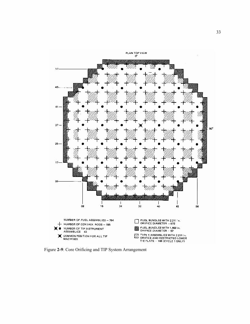
Figure 2-9: Core Orificing and TIP System Arrangement
34
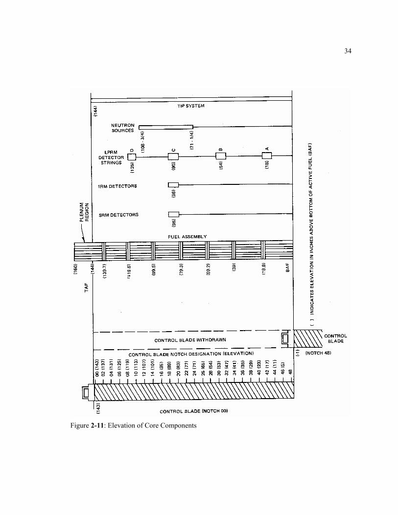
Figure 2-11: Elevation of Core Components
35
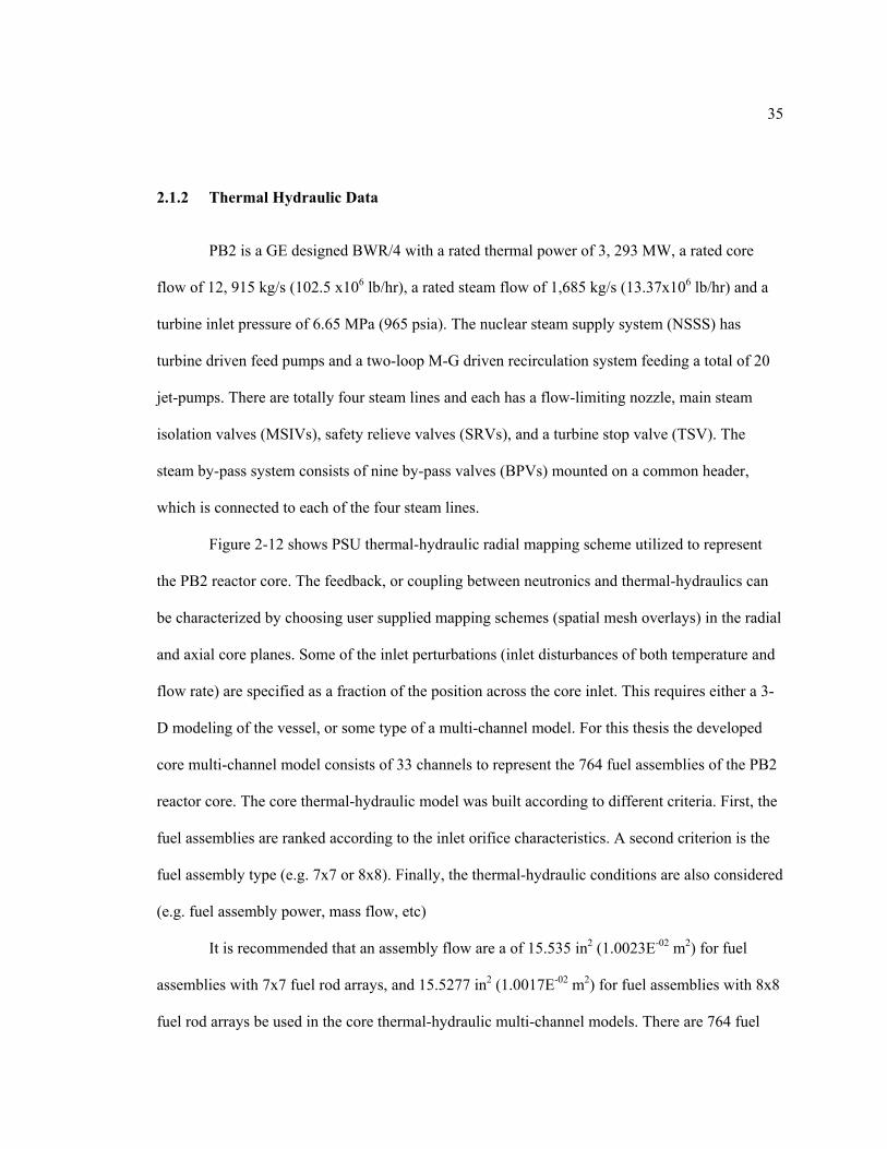
2.1.2 Thermal Hydraulic Data
PB2 is a GE designed BWR/4 with a rated thermal power of 3, 293 MW, a rated core
flow of 12, 915 kg/s (102.5 x10⁶ lb/hr), a rated steam flow of 1,685 kg/s (13.37x10⁶ lb/hr) and a
turbine inlet pressure of 6.65 MPa (965 psia). The nuclear steam supply system (NSSS) has
turbine driven feed pumps and a two-loop M-G driven recirculation system feeding a total of 20
jet-pumps. There are totally four steam lines and each has a flow-limiting nozzle, main steam
isolation valves (MSIVs), safety relieve valves (SRVs), and a turbine stop valve (TSV). The
steam by-pass system consists of nine by-pass valves (BPVs) mounted on a common header,
which is connected to each of the four steam lines.
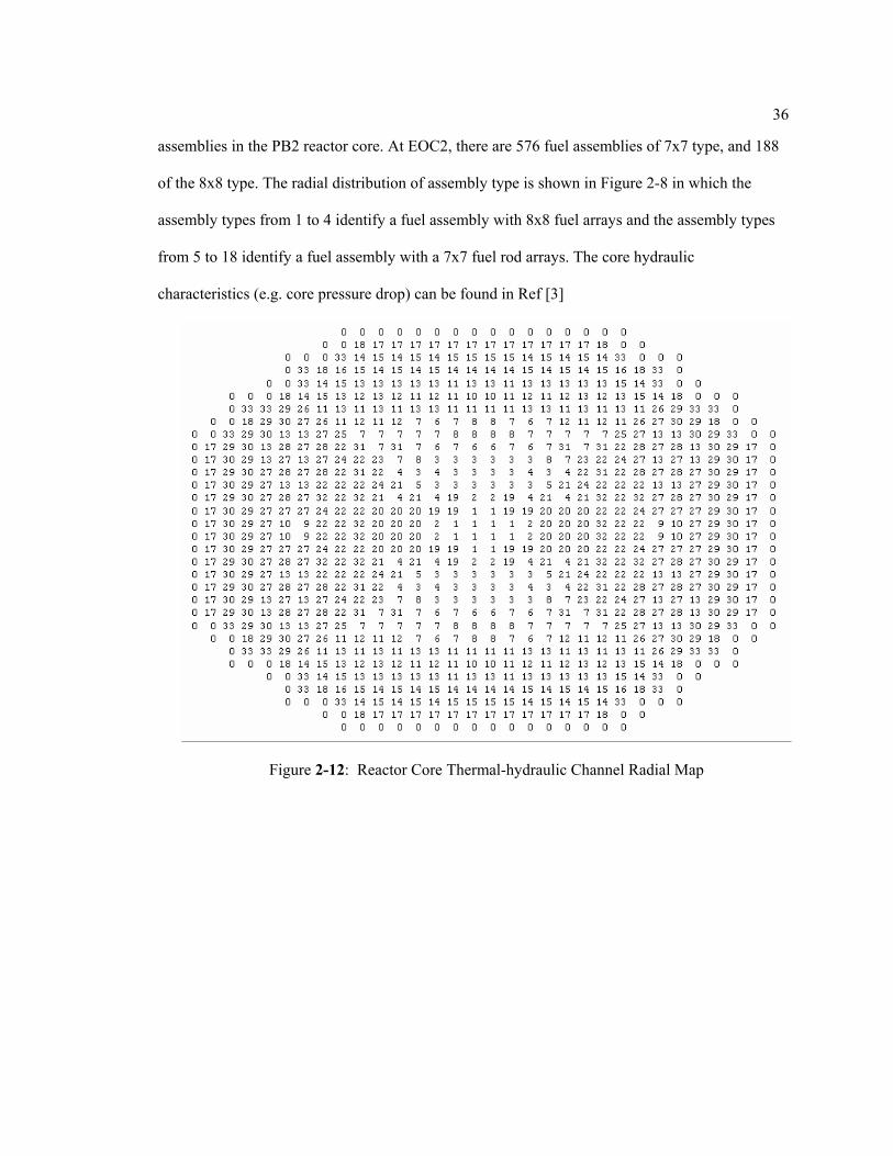
Figure 2-12 shows PSU thermal-hydraulic radial mapping scheme utilized to represent
the PB2 reactor core. The feedback, or coupling between neutronics and thermal-hydraulics can
be characterized by choosing user supplied mapping schemes (spatial mesh overlays) in the radial
and axial core planes. Some of the inlet perturbations (inlet disturbances of both temperature and
flow rate) are specified as a fraction of the position across the core inlet. This requires either a 3-
D modeling of the vessel, or some type of a multi-channel model. For this thesis the developed
core multi-channel model consists of 33 channels to represent the 764 fuel assemblies of the PB2
reactor core. The core thermal-hydraulic model was built according to different criteria. First, the
fuel assemblies are ranked according to the inlet orifice characteristics. A second criterion is the
fuel assembly type (e.g. 7x7 or 8x8). Finally, the thermal-hydraulic conditions are also considered
(e.g. fuel assembly power, mass flow, etc)
It is recommended that an assembly flow are a of 15.535 in2 (1.0023E-02 m2) for fuel
assemblies with 7x7 fuel rod arrays, and 15.5277 in2 (1.0017E-02 m2) for fuel assemblies with 8x8
fuel rod arrays be used in the core thermal-hydraulic multi-channel models. There are 764 fuel
36
assemblies in the PB2 reactor core. At EOC2, there are 576 fuel assemblies of 7x7 type, and 188
of the 8x8 type. The radial distribution of assembly type is shown in Figure 2-8 in which the
assembly types from 1 to 4 identify a fuel assembly with 8x8 fuel arrays and the assembly types
from 5 to 18 identify a fuel assembly with a 7x7 fuel rod arrays. The core hydraulic
characteristics (e.g. core pressure drop) can be found in Ref [3]
Figure 2-12: Reactor Core Thermal-hydraulic Channel Radial Map
37
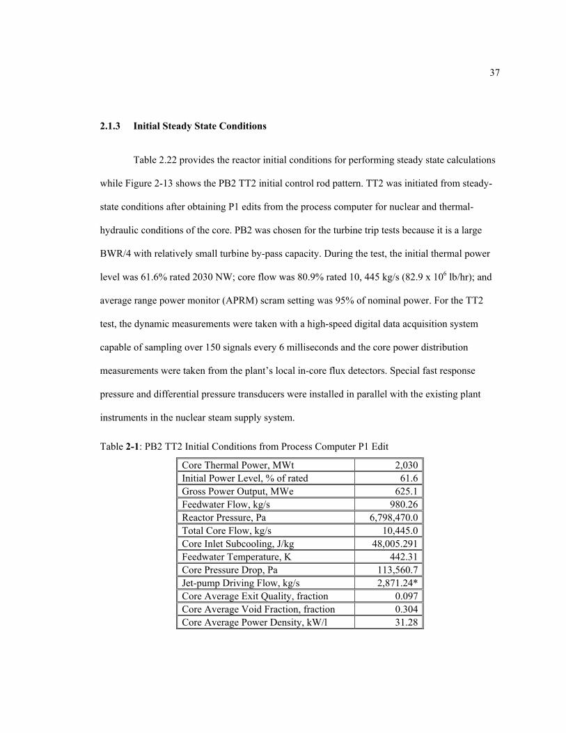
2.1.3 Initial Steady State Conditions
Table 2.22 provides the reactor initial conditions for performing steady state calculations
while Figure 2-13 shows the PB2 TT2 initial control rod pattern. TT2 was initiated from steady-
state conditions after obtaining P1 edits from the process computer for nuclear and thermal-
hydraulic conditions of the core. PB2 was chosen for the turbine trip tests because it is a large
BWR/4 with relatively small turbine by-pass capacity. During the test, the initial thermal power
level was 61.6% rated 2030 NW; core flow was 80.9% rated 10, 445 kg/s (82.9 x 10⁶ lb/hr); and
average range power monitor (APRM) scram setting was 95% of nominal power. For the TT2
test, the dynamic measurements were taken with a high-speed digital data acquisition system
capable of sampling over 150 signals every 6 milliseconds and the core power distribution
measurements were taken from the plant’s local in-core flux detectors. Special fast response
pressure and differential pressure transducers were installed in parallel with the existing plant
instruments in the nuclear steam supply system.
Table 2-1: PB2 TT2 Initial Conditions from Process Computer P1 Edit
Core Thermal Power, MWt 2,030 Initial Power Level, % of rated 61.6 Gross Power Output, MWe 625.1 Feedwater Flow, kg/s 980.26 Reactor Pressure, Pa 6,798,470.0 Total Core Flow, kg/s 10,445.0 Core Inlet Subcooling, J/kg 48,005.291 Feedwater Temperature, K 442.31 Core Pressure Drop, Pa 113,560.7 Jet-pump Driving Flow, kg/s 2,871.24* Core Average Exit Quality, fraction 0.097 Core Average Void Fraction, fraction 0.304 Core Average Power Density, kW/l 31.28

38
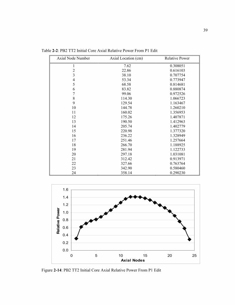
The initial water level above vessel zero (AVZ) is equal to 14.1478 m (557 in). This
measured level is the actual level inside the steam dryer shroud. The initial level AVZ is equal to
14.3256 m (564 in) for the narrow range measurement outside steam dryer shroud. AVZ is the
lowest interior elevation of the vessel (bottom of lower plenum). Table 2-23 and Figure 2-14
provide the process computer P1 edit for the initial core axial relative power distribution.
Figure 2-13: PB2 HP Control Rod Pattern
39
Table 2-2: PB2 TT2 Initial Core Axial Relative Power From P1 Edit
Axial Node Number Axial Location (cm) Relative Power
1 2 3 4 5 6 7 8 9
10 11 12 13 14 15 16 17 18 19 20 21 22 23 24
7.62 22.86 38.10 53.34 68.58 83.82 99.06
114.30 129.54 144.78 160.02 175.26 190.50 205.74 220.98 236.22 251.46 266.70 281.94 297.18 312.42 327.66 342.90 358.14
0.308051 0.616103 0.707754 0.773947 0.814681 0.880874 0.972526 1.066723 1.163467 1.260210 1.356953 1.407871 1.412963 1.402779 1.377320 1.328949 1.257664 1.188925 1.122733 1.031081 0.913971 0.763764 0.580460 0.290230
0.0
0.2
0.4
0.6
0.8
1.0
1.2
1.4
1.6
0 5 10 15 20 25Axial Nodes
Rel
ativ
e Po
wer
Figure 2-14: PB2 TT2 Initial Core Axial Relative Power From P1 Edit
40
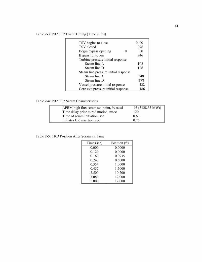
2.1.4 Transient Calculations
During the TT2 test, most of the important phenomena occur in the first five seconds of
the transient. Therefore, the test is simulated for a five-second time period. This approach
simplifies the number of components required for performing the analysis of TT2. Basically, the
transient begins with the closure of the TSV. At some point in time, the turbine BPV begins to
open. The only boundary conditions imposed in the analysis should be limited to the opening and
closure of the above valves. Table 2-24 shows the event timing during the transient. Table 2-25
shows the scram initiation time and the delay time while Table 2-26 shows the average control
rod density (CRD) position during the reactor scram. An average velocity can be obtained from
Table 2-26 for the scram modelling in the 3-D kinetics case. An approximate value obtained from
this table is 2.34 ft/s (0.713 m/s) for the first 0.04 seconds and 4.67 ft/s (1.423 m/s) thereafter.
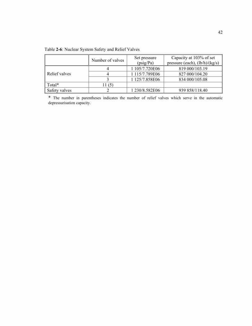
Also it should be noted that during the Exercise 3 Best Estimate Case, the set points of the SRVs
are never reached. Table 2-27 summarises the safety relief valve reference design information to
be utilized in Extreme Scenario 2.
41
Table 2-3: PB2 TT2 Event Timing (Time in ms)
TSV begins to close 0 00 TSV closed 096 Begin bypass opening 0 60 Bypass full-open 846 Turbine pressure initial response
Steam line A 102 Steam line D 126
Steam line pressure initial response Steam line A 348 Steam line D 378
Vessel pressure initial response 432 Core exit pressure initial response 486
Table 2-4: PB2 TT2 Scram Characteristics
APRM high flux scram set-point, % rated 95 (3128.35 MWt) Time delay prior to rod motion, msec 120 Time of scram initiation, sec 0.63 Initiates CR insertion, sec 0.75
Table 2-5: CRD Position After Scram vs. Time
Time (sec) Position (ft) 0.000 0.120 0.160 0.247 0.354 0.457 2.500 3.080 5.000
0.0000 0.0000 0.0935 0.5000 1.0000 1.5000 10.200 12.000 12.000
42
Table 2-6: Nuclear System Safety and Relief Valves
Number of valves Set pressure (psig/Pa)
Capacity at 103% of set pressure (each), (lb/h)/(kg/s)
4 1 105/7.720E06 819 000/103.19 4 1 115/7.789E06 827 000/104.20 Relief valves 3 1 125/7.858E06 834 000/105.08
Total* 11 (5) Safety valves 2 1 230/8.582E06 939 858/118.40
* The number in parentheses indicates the number of relief valves which serve in the automaticdepressurisation capacity.
43
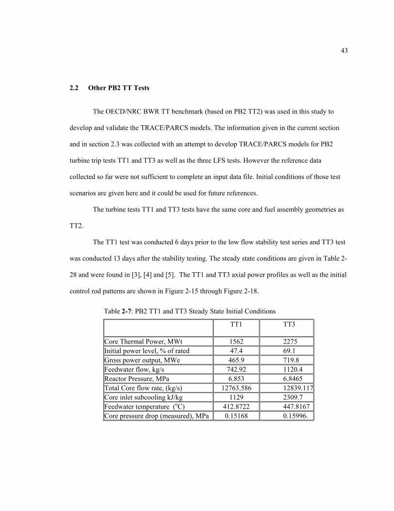
2.2 Other PB2 TT Tests
The OECD/NRC BWR TT benchmark (based on PB2 TT2) was used in this study to
develop and validate the TRACE/PARCS models. The information given in the current section
and in section 2.3 was collected with an attempt to develop TRACE/PARCS models for PB2
turbine trip tests TT1 and TT3 as well as the three LFS tests. However the reference data
collected so far were not sufficient to complete an input data file. Initial conditions of those test
scenarios are given here and it could be used for future references.
The turbine tests TT1 and TT3 tests have the same core and fuel assembly geometries as
TT2.
The TT1 test was conducted 6 days prior to the low flow stability test series and TT3 test
was conducted 13 days after the stability testing. The steady state conditions are given in Table 2-
28 and were found in [3], [4] and [5]. The TT1 and TT3 axial power profiles as well as the initial
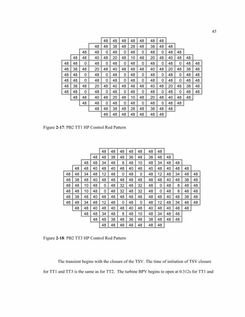
control rod patterns are shown in Figure 2-15 through Figure 2-18.
Table 2-7: PB2 TT1 and TT3 Steady State Initial Conditions
TT1 TT3
Core Thermal Power, MWt 1562 2275 Initial power level, % of rated 47.4 69.1 Gross power output, MWe 465.9 719.8 Feedwater flow, kg/s 742.92 1120.4 Reactor Pressure, MPa 6.853 6.8465 Total Core flow rate, (kg/s) 12763.586 12839.117 Core inlet subcooling kJ/kg 1129 2309.7 Feedwater temperature (oC) 412.8722 447.8167 Core pressure drop (measured), MPa 0.15168 0.15996)
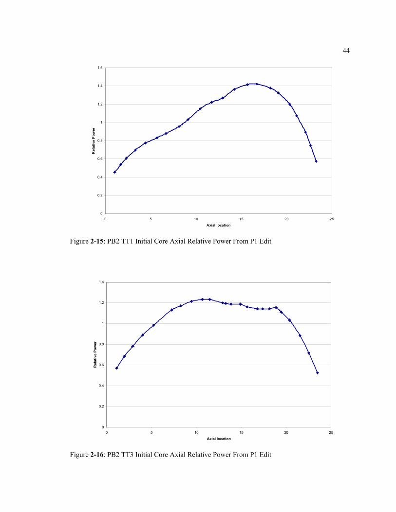
44
0
0.2
0.4
0.6
0.8
1
1.2
1.4
1.6
0 5 10 15 20 25
Axial location
Rel
ativ
e P
ower
Figure 2-15: PB2 TT1 Initial Core Axial Relative Power From P1 Edit
0
0.2
0.4
0.6
0.8
1
1.2
1.4
0 5 10 15 20 25
Axial location
Rel
ativ
e Po
wer
Figure 2-16: PB2 TT3 Initial Core Axial Relative Power From P1 Edit
45
The transient begins with the closure of the TSV. The time of initiation of TSV closure
for TT1 and TT3 is the same as for TT2. The turbine BPV begins to open at 0.312s for TT1 and
48 48 48 48 48 48 48 48 48 38 48 28 48 38 48 48 48 48 0 48 0 48 0 48 0 48 48 48 48 40 48 20 48 10 48 20 48 40 48 48 48 48 0 48 0 48 0 48 0 48 0 48 0 48 4848 38 48 20 48 40 48 48 48 40 48 20 48 38 4848 48 0 48 0 48 0 48 0 48 0 48 0 48 4848 48 0 48 0 48 0 48 0 48 0 48 0 48 4848 38 48 20 48 40 48 48 48 40 48 20 48 38 4848 48 0 48 0 48 0 48 0 48 0 48 0 48 48 48 48 40 48 20 48 10 48 20 48 40 48 48 48 48 0 48 0 48 0 48 0 48 48 48 48 38 48 28 48 38 48 48 48 48 48 48 48 48 48
Figure 2-17: PB2 TT1 HP Control Rod Pattern
48 48 48 48 48 48 48 48 48 38 48 36 48 38 48 48 48 48 34 48 8 48 10 48 34 48 48 48 48 40 48 40 48 40 48 40 48 40 48 48 48 48 34 48 12 48 0 48 0 48 12 48 34 48 4848 38 48 40 48 48 48 48 48 48 48 40 48 38 4848 48 10 48 0 48 32 48 32 48 0 48 8 48 4848 48 10 48 0 48 32 48 32 48 0 48 8 48 4848 38 48 40 48 48 48 48 48 48 48 40 48 38 4848 48 34 48 12 48 0 48 0 48 12 48 34 48 48 48 48 40 48 40 48 40 48 40 48 40 48 48 48 48 34 48 8 48 10 48 34 48 48 48 48 38 48 36 48 38 48 48 48 48 48 48 48 48 48 48
Figure 2-18: PB2 TT3 HP Control Rod Pattern
46
0.09 sec for TT3. The rate of BPV opening for TT1 and TT3 is not specified in the [3], [4] and [5]
and further information is needed. Table 2-29 shows the scram initiation time and the delay time.
Table 2-8: PB2 TT1 and TT3 Scram Characteristics
TT1 TT3 APRM high flux scram set point, % rated 85(2 799.05 MWt) 77 (2535.6 MWt)
Time delay prior to rod motion, msec 120 120
Time of SCRAM initiation 0.68 0.56
2.3 PB Low Flow Stability Tests
Multiple LFS tests were performed at PB2 BWR during the first quarter of 1977. The
tests were performed at the end of Cycle 2 with an accumulated average core exposure of 12.7
GWd/t.
The dynamic measurements were taken with a high speed digital data acquisition system
capable of sampling over 15 signals every 6 milliseconds and the core contribution measurements
were taken from the plants local in-core flux detectors. Special fast response pressure and
differential pressure transducers were installed in parallel with existing plant instruments to
measure the response of important variables in the nuclear steam supply system.
The stability tests were conducted along the low flow end of the rated power flow line,
and along the power-flow line corresponding to minimum recirculation pump speed. The reactor
core stability margin was determined from an empirical model fitted to the experimentally
derived transfer function measurement between core pressure and the APRM, average neutron
flux signals.

47
The LFS tests were intended to measure the reactor core stability margins at the limiting
conditions used in design and safety analysis, providing a one-to-one comparison to design
calculations.
2.3.1 Planning of Experiments
Four test conditions were planned to be as close as possible to one of the following
reactor operating conditions:
- points along the rated power-flow control line (PT1 and PT2)
- points along the natural circulation power – flow control line (PT2, PT3 and PT4)
- extrapolated rod-block natural circulation power-flow control line (test point PT3)
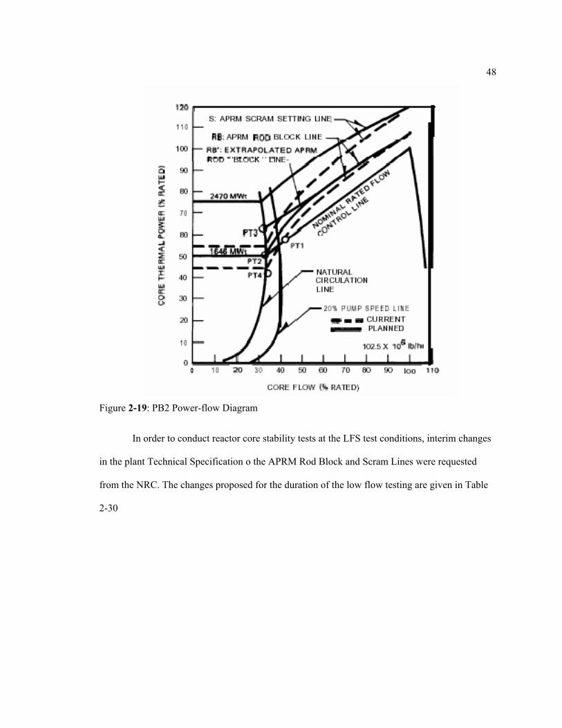
The planned test conditions are shown in Figure 2.19
48
In order to conduct reactor core stability tests at the LFS test conditions, interim changes
in the plant Technical Specification o the APRM Rod Block and Scram Lines were requested
from the NRC. The changes proposed for the duration of the low flow testing are given in Table
2-30
Figure 2-19: PB2 Power-flow Diagram
49
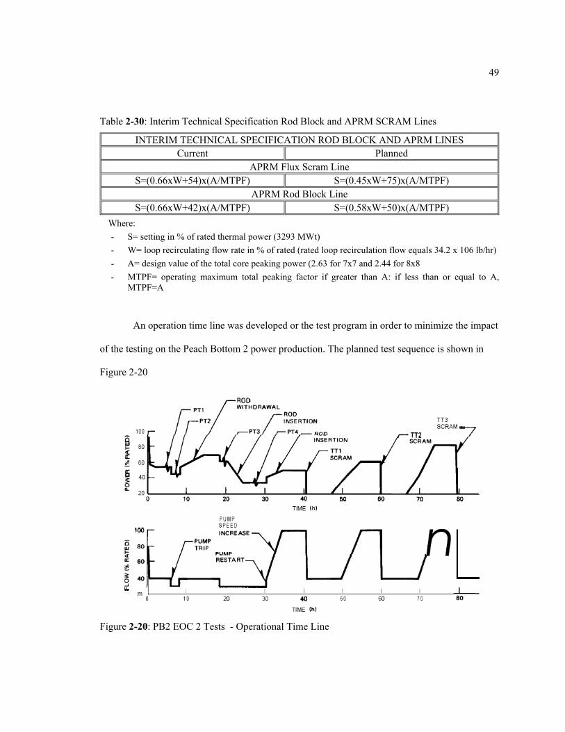
An operation time line was developed or the test program in order to minimize the impact
of the testing on the Peach Bottom 2 power production. The planned test sequence is shown in
Figure 2-20
Table 2-30: Interim Technical Specification Rod Block and APRM SCRAM Lines
INTERIM TECHNICAL SPECIFICATION ROD BLOCK AND APRM LINES Current Planned
APRM Flux Scram Line S=(0.66xW+54)x(A/MTPF) S=(0.45xW+75)x(A/MTPF)
APRM Rod Block Line S=(0.66xW+42)x(A/MTPF) S=(0.58xW+50)x(A/MTPF)
Where: - S= setting in % of rated thermal power (3293 MWt) - W= loop recirculating flow rate in % of rated (rated loop recirculation flow equals 34.2 x 10⁶ lb/hr)- A= design value of the total core peaking power (2.63 for 7x7 and 2.44 for 8x8 - MTPF= operating maximum total peaking factor if greater than A: if less than or equal to A,
MTPF=A
Figure 2-20: PB2 EOC 2 Tests - Operational Time Line
50
The reactor was maneuvered by setting the desired fixed control rod pattern and by using
flow control. The strategy was to conduct the tests on a tightly controlled time schedule which
allowed for the xenon transient effects. By testing the maxima or minima xenon concentration,
the waiting time for stable power level and flux distribution in the core could be reduced from 24
to 5 hours prior to each test.
During the Peach Bottom 2 testing, unforeseen changes in plant operation and utility load
demand dictated some modifications of the planned test sequence shown in Figure 2-19.
2.3.2 Actual Test Conditions
The actual reactor operating conditions at which the low-flow core stability testing was
conducted is listed in Table 2-31.
PT1 PT2 PT3 PT4
Core Thermal Power, MWt 1995.00 1702.00 1948.00 1434.00 Initial Power Level,% of rated 60.6 51.7 59.2 43.5 Total Core Flow, kg/s 6753.60 5657.40 5216.40 5203.8 Total reactor flow, % of rated 51.3 42.0 38.0 38.0 Reactor Steam Dome Pressure, Pa 6860286 6814781 6904413 6863044 Core exit pressure, Pa 7063682 7008689 7098052 7056808 Core Inlet Enthalpy, kJ/kg 1183.610 1187.78 1184.610 1183.83 Core Inlet Subcooling, kJ/kg 75.160 79.648 77.442 76.075 Core Inlet Temperature, oC 270.11 270.73 270.09 269.96 Feed Water Mass Flow, kg/s 963.90 808.92 941.22 671.58
The strong effect of the xenon transient occurring during the stability testing can be
determined from a plot of the test conditions on a power flow map in Figure 2-19. The skewing of
the rated rod line between test conditions PT1 and PT2 from the equilibrium xenon calculated
Table 2-31: Actual Low-Flow Stability Test Conditions

51
line gives an indication of the effect of the xenon transient. The average axial power distribution
in the core was found to be stable following the xenon soak (Hourly tests of the average axial
power distribution indicated local power changes of less than 0.5 % taking place).
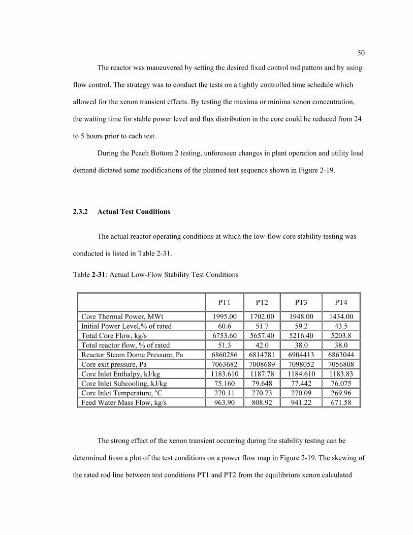
The control rod patterns and axial power distributions obtained from the four PB2 EOC 2
low flow stability tests PT1, PT2, PT3 and PT4 are shown in Figure 2-21 through 2-28.
Figure 2-21: PB2 EOC 2 PT1 Test – Control Rod Pattern
52
Figure 2-22: PB2 EOC 2 PT1 Test - Average Axial Power Distribution
Figure 2-23: PB2 EOC 2 PT2 Test – Control Rod Pattern
53
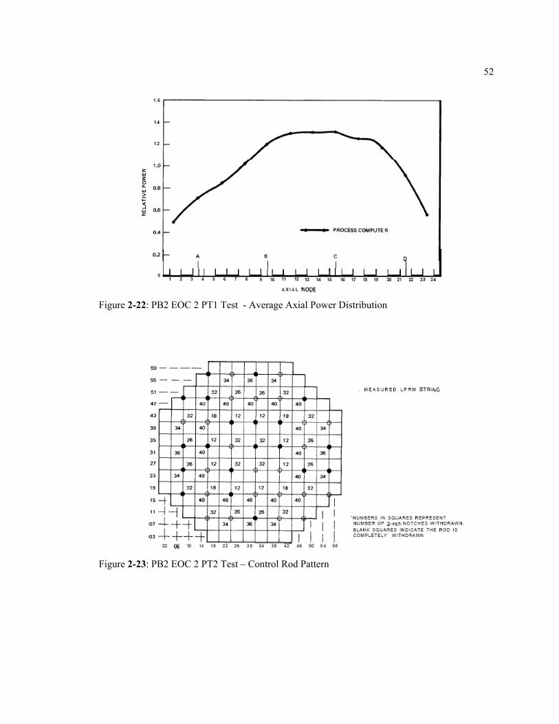
Figure 2-24: PB2 EOC 2 PT2 Test - Average Axial Power Distribution
Figure 2-25: PB2 EOC 2 PT3 Test – Control Rod Pattern
54
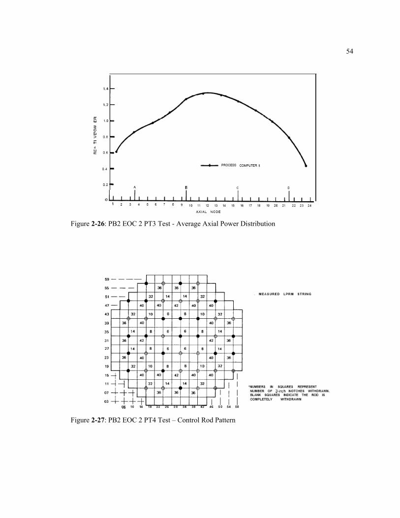
Figure 2-26: PB2 EOC 2 PT3 Test - Average Axial Power Distribution
Figure 2-27: PB2 EOC 2 PT4 Test – Control Rod Pattern
55
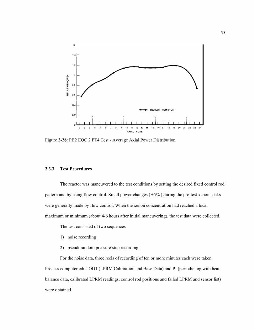
2.3.3 Test Procedures
The reactor was maneuvered to the test conditions by setting the desired fixed control rod
pattern and by using flow control. Small power changes ( 5%± ) during the pre-test xenon soaks
were generally made by flow control. When the xenon concentration had reached a local
maximum or minimum (about 4-6 hours after initial maneuvering), the test data were collected.
The test consisted of two sequences
1) noise recording
2) pseudorandom pressure step recording
For the noise data, three reels of recording of ten or more minutes each were taken.
Process computer edits OD1 (LPRM Calibration and Base Data) and PI (periodic log with heat
balance data, calibrated LPRM readings, control rod positions and failed LPRM and sensor list)
were obtained.
Figure 2-28: PB2 EOC 2 PT4 Test - Average Axial Power Distribution
56
Two TIPs were then set at symmetric locations in the core, the first at [ ]117 cm∼ and the
second at [ ]178 cm∼ above the bottom.
The pseudorandom pressure step recording was preceded by preliminary trial pressure
steps. First, a single pressure step was run. The signal-to-noise level was examined and, if not
adequate, the step size was increased in small increments of about 0.17 bars until the signal-to-
noise level was satisfactory. Usually a 0.55 bars step was adequate. Then, with the reactor
operator concurrence, a pseudorandom stepping sequence (down, then up) was run with a
sampling interval of 1 second. Three reels of 10 to 20 minutes of data were taken.
The perturbation data were evaluated to verify that the following criteria had been met:
1) maximum APRM response for pressure set point steps was less than 220 % of rated
(checked prior to start of stepping sequence);
2) the decay ratio was less than 1.0 for each process variable that exhibits oscillatory
response to pressure set points;
3) the daily off gas increase did not exceed 50% of the unit release rate prior to
beginning testing (release rate 1 hour after test had to be less than 150% of release
rate prior to start of test)
2.3.4 Adopted Transient Analyses
Two types of transient perturbation have been investigated with the objective to study the
reactor behavior within the stability region of the Power/Flow Map. These are Control Rod (CR)
perturbation and pressure perturbation. All the analyses performed reproduce cases than can
normally occur in a BWR reactor, more specifically, the disturbances applied in the several tests
are similar to the perturbations used in the reference tests.

57
The various analyses have also been intended to demonstrate the reliability of using small
pressure perturbation tests to determine the stability margin of a large BWR code.
The CR perturbation is actuated by changing the PARCS input deck related to the
Control Rod position at the beginning of the transient, i.e. end of coupled steady state calculation.
As a consequence the cross sections provide variations of their compositions which of course
cause a reactivity variation and power oscillations.
The pressure perturbation is actuated by the Turbine Control Valve. The applied
perturbation was a triangular variation of the TCV flow area in 0.2 sec and magnitude of 0.055
MPa.
58
Chapter 3
TRACE/PARCS Code Description and Model Development
The calculation analyses described in this thesis involve the applications of simulation
tools such as thermal hydraulics system code TRACE and 3-D neutron kinetics code PARCS and
the coupling between the two. This chapter is focused on their description as well as the
approximations made during the analysis and their justification. The description begins with
detailed information in regards to TRACE [8], followed by a description of PARCS [9]. The low
flow stability tests require the utilization of a special tool DRARMAX [10]. DRARMAX is a
post-processing code, which was developed at Purdue University and is applied to evaluate the
decay ratio (DR) and natural frequency (NF) from the time series output of the TRACE/PARCS
calculation.
3.1 Thermal-hydraulics System Code TRACE
TRACE (TRAC RELAP5 Advanced Computational Engine) code is a US NRC reactor
system analysis code [8]. It is designed to perform best-estimate analysis of loss-of-coolant
accidents (LOCAs), operational transients, and other accident scenarios in Pressurized Water
Reactors (PWR) and Boiling Water Reactors (BWRs). Experimental facilities and fluid
phenomena occurring in them are also within the range of simulation abilities of the code. Models
applied in the code include multidimensional two-phase flow, non-equilibrium thermo-dynamics,
generalized heat transfer, reflood, level tracking, and reactor kinetics. The code also provides
automatic steady-state and dump/restart capabilities.
59
3.1.1 TRACE Field Equations
TRACE uses two-fluid, two-phase field equation set based on single phase Navier-Stokes
equations for each phase, and jump conditions between the phases. It consists of separate mass,
energy, and momentum conservations for the liquid and gas fields which defines six partial
differential equations (PDEs). The components of non-condensable gas in the system and its
mixture with steam are assumed to move at the same velocity and temperature. As a result a
single momentum equation and a single energy equation are used for the gas mixture. Relative
concentrations of steam and non-condensables are determined by using separate equations for
each component of the gas field. For example, TRACE permits users to treat nitrogen and air as
two separate components of gas field (two additional mass equations), and allows requests for
more non-condensable equations if needed (e.g. hydrogen). The set of field equations can be
further extended if a user chooses to follow the boron concentration in the system.
Time and volume averaging is applied to this combination of equations, to obtain a useful
set of two-fluid, two phase conservation equations. TRACE uses this flow model in both one and
three dimensions. Detailed description of the TRACE field equations are given in [8]
The TRACE code invokes a quasi-steady approach to the heat-transfer coupling between
the wall and the fluid as the closure relations for interfacial and wall-to-fluid heat transfer and
drag. This approach assumes detailed knowledge of the local fluid parameters and ignores time
dependencies so that the time rate of change in the closure relationships becomes infinite and the
time constants are zero. It has the advantages of being reasonably simple (and, therefore generally
applicable to a wide range of problems) and not requiring previous knowledge of a given
transient. Where appropriate, the quasi-steady methodology presented in this chapter is somewhat
limited. Detailed description of the quasi-steady approach is given in [8].
60
The partial differential equations are solved using finite volume numerical method. The
heat transfer equations are evaluated using a semi-implicit time-differencing technique. The fluid-
dynamics equations in the spatial one-dimensional (1D), and three-dimensional (3D) components
use, by default, a multi-step time-differencing procedure that allows the material Courant-limit
condition to be exceeded. A more straightforward semi-implicit time-differencing method is also
available. The finite difference equations for hydrodynamic phenomena form a system of
coupled, nonlinear equations that are solved by the Newton-Raphson iteration method. The
resulting linearized equations are solved by direct matrix inversion. For the 1D network matrix,
this is done by a direct full-matrix solver; for the multiple-vessel matrix, this is done by the
capacitance-matrix method using a direct banded-matrix solver.
TRACE takes a component-based approach to modeling a reactor system. Each physical
piece of equipment in a flow loop can be represented as some type of component, and each
component can be further nodalized into some number of physical volumes (also called cells)
over which fluid, conduction and kinetics equations are averaged. The number of reactor
components in the problem and the manner in which they are coupled is arbitrary. There is no
built-in limit for the number of components or volumes that can be modeled; the size of a
problem is theoretically only limited by the available computer memory. Reactor hydraulic
components in TRACE include PIPEs, PLENUMs, PRIZERs (pressurizers), CHANs (BWR fuel
channels), PUMPs, JETPs (jet pumps), SEPD (separators), TEEs, TURBs (turbines), HEATRs
(feedwater heaters), CONTANs (containment), VALVEs, and VESSELs (with associated
internals). HTSTR (heat structure) and REPEAT-HTSTR components modeling fuel elements or
heated walls in the reactor system are available to compute two-dimensional conduction and
surface-convection heat transfer in Cartesian or cylindrical geometries. POWER components are
available as a means for delivering energy to the fluid via the HTSTR or hydraulic component
walls. FLPOWER (fluid power) components are capable of delivering energy directly to the fluid
61
(such as might happen in was transmutation facilities). RADENC (radiation enclosures)
components may be used to simulate radiation heat transfer between multiple arbitrary surfaces.
Fill and BREAK components are used to apply the desired coolant-flow and pressure boundary
conditions, respectively, in the reactor system to perform steady-state and transient calculations.
EXTERIOR components are available to facilitate the development of input models designed to
exploit TRACE’s parallel execution features.
3.2 Neutron Kinetics Code PARCS
PARCS is a three-dimensional (3D) reactor core simulator which solves the steady-state
and time-dependent, multigroup neutron diffusion and SP3 transport equations in orthogonal and
non-orthogonal geometries. PARCS is coupled directly to the thermal-hydraulic system code
TRACE which provides the temperature and flow field information to PARCS during the
transient calculations via the few group cross sections. A separate code module, GENPMAXS, is
used to process the cross sections generated by a lattice physics code into the PMAXS format that
can be read by PARCS.
Since the initial release of the NRC version of PARCS (v1.01) in November 1998, there
have been numerous functional improvements and code feature extensions [11, 12]. The major
calculation features in PARCS include the ability to perform eigenvalue calculations, transient
(kinetics) calculations, Xenon transient calculations, decay heat calculations, pin power
calculations, and adjoint calculations for commercial Light Water Reactors. The primary use of
PARCS involves a 3D calculation model for the realistic representation of the physical reactor.
However various one dimensional (1D) modeling features are available in PARCS to support
faster simulations for a group of transients in which the dominant variation of the flux is in the
axial direction, as for example in several BWR applications.
62
A card name based input system is employed in PARCS such that the use of default input
parameters is maximized and the amount of the input data is minimized. A restart feature is
available to continue the transient calculation from the point where the restart file was written.
Various edit options are available in PARCS to show many different aspects of the calculation
results. The online graphics features of PARCS provide a quick and versatile visualization of the
various physical phenomena occurring during the transient calculation.
Numerous sophisticated spatial kinetics calculation methods have been incorporated into
PARCS in order to accomplish the various tasks with high accuracy and efficiency. For example,
the Coarse Mesh Finite Difference (CMFD) formulation provides a means of performing a fast
transient calculation by avoiding expensive nodal calculations at times in the transient when there
is no strong variation in the neutron flux spatial distribution. The temporal discretization is
performed using the theta method with an exponential transformation of the group fluxes. A
transient fixed source problem is formed and solved at each time point in the transient. For
special discretization, a variety of solution kernels are also available to include the most popular
LWR two group nodal methods, Analytical Nodal Method (ANM) and Nodal Expansion Method
(NEM).
Advanced numerical solution methods are used in PARCS in order to minimize the
computational burden. The solution of the CMFD linear system is obtained using a Krylov
subspace method which utilizes a BILU3D preconditioner. The eigenvalue calculation to
establish the initial steady-state is performed using the Wielandt eigenvalue shift method. When
using the two group nodal methods, a pin power reconstruction method is available in which
predefined heterogeneous powers from functions are combined with a homogenous intranodal
distribution.

63
PARCS is also capable of performing core depletion analysis. Burnup dependent
macroscopic sections are read from the PMAXS file prepared by the code GENPMAS and the
PARCS node-wise power is used to calculate the region-wise burnup increment for time
advancing the macroscopic cross sections. Details of the PMAXS file and the GENPMAXS code
are provided in the GENPMAXS manual.
PARCS was written in FORTRAN 90 and its portability has been tested on various
platforms and operating systems, to include SUN Solaris UNIX, DEC ALPHA UNIX, HP UNIX,
LINUX, and various Windows OS (i.e. 95, 98, NT and 2000). Because of its various functional
features, PARCS can be run in numerous execution modes. The following section will first
provide a brief overview of the important PARCS user features.
3.2.1 Calculation Features
PARCS is equipped with various calculation modules needed to predict the global and
local response of the reactor in steady-state and transient conditions. The various features of
PARCS are described in this section along with the corresponding modules.
Eigenvalue Calculation
In order to establish the initial steady state, it is necessary to perform an eigenvalue
calculation. PARCS performs the eigenvalue calculation using the Wielandt eigenvalue shift
method. The eigenvalue obtained is used to adjust the nu ( )ν values in the subsequent transient
calculation in order to make the initial reactor state critical. In addition to the standard k-eff
calculation for a given reactor configuration, the critical boron concentration (CBC) search
function is available. The type of search is defined in the SEARCH card of the CNTL block
input.
Transient (Kinetics) Calculation
This is primary function of PARCS that solves the time-dependent neutron diffusion
equation involving both delayed and prompt neutrons. . The transient calculation option is turned
64
on and off by the TRANSIENT card in the CNTL block. The temporal differencing based on the
exponential transform and the theta method yields a transient fixed source problem at each time
step. The fixed source problem is solved using the Coarse Mesh Finite Difference (CMFD)
method in which a conditional nodal update scheme is employed. The temporal discretization
schemes can be specified by the THETA and EXPO_OPT cards in the TRAN input block.
Exponential extrapolation can be sued to obtain an initial flux guess at each new time step by
activating this option in the expo_opt card. The conditional nodal update scheme activates the
higher order nodal update only when there are substantial local cross section changes. The
conditional nodal update is controlled by the EPS_XSEC card in the TRAN block.
Xenon Transient Calculation
For slow reactor transients, it is essential to provide a Xenon transient capability. In
PARCS, the conventional quasi-static treatment of xenon transients is used that employs the
eigenvalue problem solver instead of the transient fixed source problem. The number densities of
Xenon and Samarium are updated by solving the respective balance equations using the fluxes
resulting from the eigenvalue calculation. The Xenon option is controlled in the XE_SM card in
the CNTL block by choosing one of the following options: 1)No Xenon, 2) Equilibrium Xenon,
or 3) Transient Xenon.
Decay Heat Calculation
A simplified decay heat model involving six groups of decay heat precursor groups is
employed in PARCS. The 6 group decay heat precursor equation is treated in the same way as the
delayed neutron precursor equation. The solution of the precursor equation is thus node wise and
provides at each time step the decay heat to sum with the fission power in order to determine the
total power produced in each node. Default values of the precursor fractions and decay constants
of the 6 groups are provided for UO2 fueled cores which are operated for a sufficiently long
period of time. The option exists for the user to specify alternate values for the precursor fractions
65
and decay constants. The decay heat option is specified in the DECAY_HEAT card in the CNTL
block and the input parameters are specified in the DHP_BETA and DHP_LAMBDA cards in the
XSEC block.
Pin Power Calculation
The primary dependent variables in PARCS are the node average fluxes and interface
currents. In order to obtain local pin power distributions, it is thus necessary to “reconstruct” pin
powers. This is performed in PARCS by multiplying the heterogeneous power form functions
with the homogeneous intra-nodal flux distribution. The homogeneous intra-nodal flux is
calculated by performing an analytical solution of a 2D fixed source problem in which the surface
average currents are specified at the four boundaries. The surface average currents are obtained
from the converged node average flux distribution at a given state. Pin power reconstruction is
performed for both the steady-state and transient condition. The pin power calculation option is
activated by the PIN_POWER card in the CNTL block and the heterogeneous power form
functions are supplied via the PFF block. Corner discontinuity factors can be used to enhance the
accuracy of the pin power distribution and can be specified in the CDF card in the XSEC block.
In order to save computing time for the pin power calculation in the PINCAL_LOC card of the
GEOM block. The transient pin power calculation needs not to be performed at every time step
since the pin-to-box factor does not change appreciably unless there is a substantial change in the
core configuration. The transient pin power calculation frequency is activated by the PIN_FREQ
card in the TRAN block.
Modeling Features
One of the essential neutronics problems for a reactor core is to represent the physical
system with an accurate numerical model. Among the various fundamental modeling issues in the
reactor kinetics calculation are the geometric representation, the cross section representation, and
the thermal-hydraulic (T-H) feedback modeling. PARCS provides a 3 D geometric representation
66
of the core that can be reduced to 2D, 1D, or 0D by the choice of the appropriate boundary
conditions. However, a special 1D kinetics capability is also available for more accurate and
versatile 1D modeling. Various geometric representation features will be described in the first and
fourth subsections below. The basic cross section representation scheme in PARCS is to
functionalize the macroscopic cross sections with linear or quadratic dependence on the T-H state
variables. The details of the PARCS cross section representation scheme are provided in the
second subsection. Thermal-hydraulically, PARCS uses an external T-H solver which greatly
extends its range of applicability. The original T-H solver of PARCS is intended primarily for
code testing and not for practical applications, and therefore only the external T-H features are
detailed in third subsection. The input description for the internal T-H solver is still provided
since PARCS continues to process this block.
Geometric Representation
In PARCS, the reactor core is modeled by a group of homogeneous computational nodes.
Radially, the computational node can be either rectangular or hexagonal. The size of the node is
of the order of fuel assembly pitch, while axially the size is 10~30 cm. In the rectangular option,
the core geometry is specified in the GEOM block, whereas the block name is changed to
GEOMH for the hexagonal option. The core radial configuration is specified using the unity of a
fuel assembly by the RAD_CONF card in GEOM block. The radial node size is then specified by
the number of subdivisions of the assembly node by the NEUTMESH_X and NEUTMESH_Y
cards. So the number of nodes per assembly can be freely chosen as nsubx*nsuby. Normally, one
or four nodes per assembly are used for practical calculations. However, it is possible to perform
a fine mesh calculation using the geometry input structure. Also by taking the assembly-wise
configuration as the pin-wise configuration, a pin-by-pin heterogeneous core representation is
also possible. The refined geometry feature is, however limited to the rectangular case only. In
67
the hexagonal case, a hexagon is always represented with one node although internally it is
divided into 6 triangular nodes within the TPEN kernel.
Cross section Functionalization
PARCS uses macroscopic cross sections which can be input in either the two group of
multi-group form using the same input cards. The macroscopic nodal cross sections are
functionalized in terms of boron concentration (B, in ppm), square root of fuel temperature,
moderator temperature and densities, void fraction and the effective rodded fractions. Only the
linear dependence of cross sections is considered on these state variables except for the moderator
density and void fractions for which the quadratic variation is provided. Symbolically, the cross
sections are functionalized as
( )( ) ( )
( ) ( )0 1 0 2 0 3 0
2 24 0 5 0 6 7
, , , , ,f m m
f f m m
m m m m CR
B T T D
a B B a T T a T T
a D D a D D a a
α ξ
α α ξ
Σ =
Σ + − + − + − +
+ − + − + + + ∆Σ
(3.1)
Here the effective rodded fraction is defined as the product of the volumetric rodded
fraction and the flux depression factor that is computed by the de-cusping routine for the partially
rodded node. For Xenon calculations, the Xenon and Samarium microscopic cross sections are
represented in the same form.
Currently, a few special benchmark cross section representation types are available: e.g.
for the OECD PWR MSLB (Main Steam Line Break) problem, for the OECD BWR PBTT
(Peach Bottom Turbine Trip) problem, and for the OECD VVER 1000 Coolant Transient CT-1
problem.
Thermal-Hydraulics Feedback
PARCS is coupled with the thermal-hydraulics code TRACE by the EXT_TH card in the
CNTL block. The coupling between PARCS and the TRACE code is achieved by the inter-
68
process protocol, PVM. The two processes are loaded in parallel and the PARCS process
transfers the nodal power data to the T-H process. The T-H process then sends back the
temperature (fuel and coolant) and density data back to the PARCS process. Originally, it was
necessary to execute a third intermediate process, General Interface (GI), which manages the data
transfer between the two processes. But this process has been integrated into PARCS so that only
two processes are to be run in parallel. Currently TRACE uses PARCS as a library of subroutines,
eliminating the need for parallel communications links.
In general the neutronics spatial mesh/node structure is different from the T-H spatial
mesh/node structure. The difference is to be mitigated by a proper mapping scheme (spatial mesh
overlays). This mapping used to be explicit in that the fractions of different T-H nodes belonging
to a neutronic node had to be specified in a file called MAPTAB for all the neutronic nodes. In
order to reduce the user effort to prepare the MAPTAP file, automatic mapping scheme were
developed for the coupled TRACE/PARCS code that take data from both PARCS and TRACE
input files to generate mapping information internally.
The time step used in system T-H calculations is often small because of stability
consideration. Some times it is so small that no significant changes occur in the core T-H
condition and performing a neutronic calculation with such a small change would be wasteful
since the neutronics solution does not change much either. In order to circumvent this
inefficiency, a skip factor can be used in the coupled calculation such that the T-H code calls
PARCS based on this user defined frequency. Different skip factors can be specified for the
steady state and transient calculation in the EXT_TH card.
Core Depletion Analysis
PARCS performs macroscopic core depletion analysis by time advancing burnup
dependent macroscopic cross sections. The PARCS node-wise power is used to calculate the
region-wise burnup increment which is then used to update the macroscopic cross sections using
69
the PMAXS cross section file. The assembly-wise history effects (e.g. moderator density history,
control rod history) are also treated using the local burnup dependence.
The depletion capability was added to the PARCS code in version 2.5. A macroscopic
depletion module adds the following functions to PARCS:
1) Ability to read in the macroscopic cross sections from PMAXS, the XS file
prepared by the interface code GENPXS.
2) Ability to calculate region wise macroscopic cross sections as a function of the
history state, such as burnup, moderate density history, control rod history.
3) Ability to calculate region wise burnup increment at each step based on the
region wise fluxes
The depletion module was implemented in PARCS by inserting several entry points in
the code. The depletion module is activated in PARCS using the input block DEPL which is
described in the user input. Utilization of the depletion option also requires the use of the two
cards in the CNRL block and four cards in the T_H block
3.3 TRACE/PARCS Coupled Methodology
When T_H conditions for PARCS are provided by an external system code (e.g.
TRACE), the temperature/fluid condition required at each neutronics node for the feedback
calculation consists of the coolant density/temperature and the effective fuel temperature. The
nodal power information determined by PARCS is then transferred back to the system code.
During the course of data transfer, the difference in the neutronic and T-H nodalizations are
reconciled by the mapping scheme described below.
In general, coarser node sizes are used in the core T-H calculation than in the PARCS
neutronics calculation. Therefore, a T-H node usually consists of several neutronics nodes.
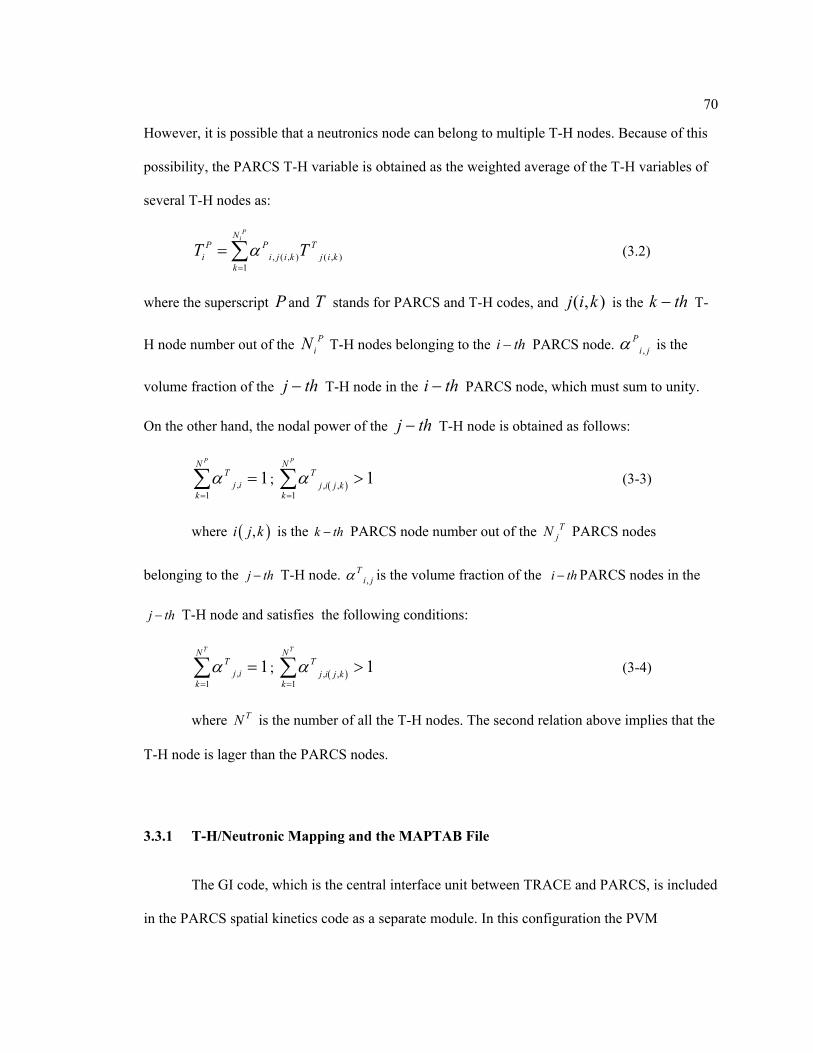
70
However, it is possible that a neutronics node can belong to multiple T-H nodes. Because of this
possibility, the PARCS T-H variable is obtained as the weighted average of the T-H variables of
several T-H nodes as:
, ( , ) ( , )1
PiN
P P Ti i j i k j i k
kT Tα
=
= ∑ (3.2)
where the superscript P and T stands for PARCS and T-H codes, and ( , )j i k is the k th− T-
H node number out of the PiN T-H nodes belonging to the i th− PARCS node. ,
Pi jα is the
volume fraction of the j th− T-H node in the i th− PARCS node, which must sum to unity.
On the other hand, the nodal power of the j th− T-H node is obtained as follows:
,1
1PN
Tj i
kα
=
=∑ ; ( ), ,1
1PN
Tj i j k
kα
=
>∑ (3-3)
where ( ),i j k is the k th− PARCS node number out of the TjN PARCS nodes
belonging to the j th− T-H node. ,T
i jα is the volume fraction of the i th− PARCS nodes in the
j th− T-H node and satisfies the following conditions:
,1
1TN
Tj i
kα
=
=∑ ; ( ), ,1
1TN
Tj i j k
kα
=
>∑ (3-4)
where TN is the number of all the T-H nodes. The second relation above implies that the
T-H node is lager than the PARCS nodes.
3.3.1 T-H/Neutronic Mapping and the MAPTAB File
The GI code, which is the central interface unit between TRACE and PARCS, is included
in the PARCS spatial kinetics code as a separate module. In this configuration the PVM

71
communication between PARCS and the GI has been replaced with direct data copy logic, and
the GI continues to manage all PVM communication with TRACE. Thus, two processes (TRACE
and PARCS) need to be executed. In addition to this merging of the GI into PARCS, an automatic
mapping kernel for the GI has been designed and implemented. This kernel is currently able to
manage the following mapping configurations:
(1) Cylindrical T-H volumes from the TRACE vessel component to Cartesian neutronics
nodes, where no mapping information is specified. The weighting factors are computed based
strictly on geometric union of the cylindrical T/H grid and the Cartesian neutronic grid.
(2) Cylindrical T-H volumes from the TRACE vessel component to Cartesian neutronics
nodes, where a radial map is used to explicitly specify which radial T-H cell should be coupled to
which neutronic node. Specifying this radial map allows the user to bypass the mapping logic
which computes weighting fractions based on strictly on the geometric union of the T/H and
Neutronic grids.
(3) Multiple BWR CHAN components to a 3 D neutronic core. This functionality
requires that the user input a radial map which specifies the CHAN(s) to be coupled to each
neutronic node and with what weighting factor. It is the responsibility of the user to ensure that
the geometric volume of each T-H CHAN is consistent with the number of neutronic nodes to
which it is coupled.
(4) BWR CHAN component(s) to a 1D neutronic core. This scenario arises from
calculations performed with either a TRAC-BF1 input deck (where PARCS processes the 1D
kinetics data from the TRAC-BF1 deck and thus does not need a separate PARCS input deck or
“MAPTAB” file), or a TRACE deck (where PARCS must process the 1D kinetics data from its
own input deck and a “MAPTAB” file is required).
The auto-mapping kernel works for calculations involving both old and new TRACE heat
structure formats, and no changes to the PARCS input deck or the “MAPTAB” file are required.
72
The radial mapping for volumes and heat structures is performed based on one of the mapping
configurations listed above, and the axial mapping is performed without user intervention. For the
axial mapping, a linear interpolation scheme is used for both the hydraulics cells and the heat
structures, which provides a fluid/fuel temperature distribution in the channel which is more
accurate than without interpolation. For the mapping of axial hydraulic cells, it is assumed that
the fluid conditions exist at the exit of the cell.
The tabular weighting factors required in previous “MAPTAB” files are now no longer
necessary. If this data is not input, or if only a radial map is specified, the code will assume that
automatic mapping is to be performed. However, if this tabular data is present in the “MAPTAB”
file, the auto-mapping logic will be deactivated, and the input weighting factors will be used.
Most 1D routines were written in FORTRAN 90 to take advantage of dynamic memory
allocation and derived data types. The 1D module thus has different memory addresses even
through the same variable names are used as in the 3D routines. Due to the use of dynamic
memory allocation, no 1D memory will be allocated during the normal 3D runs so that the
addition of the 1D routine will not harm the execution of the 3D module.
The input/output (I/O) formats of the 1D module were made consistent with the 3D
module in order to minimize newly defined input cards and also to provide convenient user
accessibility. When the 1D module is invoked, the input data necessary for the 1D module is
transferred from 3D common blocks to 1D common blocks. After that the 1D module is
independently executed in the normal calculation mode without triggering any 3D routines.
3.4 DRARMAX
The post processing code, DRARMAX, which was developed at Purdue University, is
selected to evaluate the DR and NF from the time series output of the TRACE/PARCS
73
calculation. DRARMAX evaluates the decay ratio and the natural frequency for signals obtained
from transients initiated by short perturbations as well as those obtained from noise simulation
during stationary operation. DRAMAX is able to calculate the DR and NF taking into
consideration also the signal constituting the perturbation given to the system. DRARMAX also
determines DRs and NFs for three types of functions: the output signal, its autocorrelation
function (ACF) and the impulse response function (IRF). For each of the three types of functions
DRARMAX fits the function with a damped sinusoidal form:
0( ) cos( )tx t c ce tα ω ϕ−= + + (3-5)
The first xx seconds of the calculated time trace are not used for the fit because they have
contamination from higher order modes and the particular shape of the perturbation used. If least
square fitting is successful, the DR and the NF are given as:
2 /fDR e πα ω−= (3-6)
/(2 )fFr ω π= (3-7)
The definition of DR and NF is appropriate for transients with short perturbation, such as
control rod and pressure perturbations.
For the measured or simulated noise signals, DRARMAX code will first extract the
impulse response function (IRF) by an autoregressive and moving average (ARMA) process [14].
1 0( ) ( ) ( )
p q
k mk m
x i a x i k b u i m= =
= − − + −∑ ∑ (3-8)
where ,u x are input and output noise signals, ,p q are orders of the ARMA process, and
coefficients ,k ma b are obtained by the prediction-error identification method (PEM). An index
referred to as Final Prediction Error (FPE) is defined to estimate the quality of the ARMA model:
1 ˆ|| ||2 1
N qFPE x xN p q
+ += −
− − − (3-9)
74
where N is the number of sampled data points and x̂ is approximation of the output signal by
ARMA.
The Lyapunov DR and NF are used for noise signals:
2 Re( ) / Im( )LDR e π γ γ−= (3-10)
Im( ) /(2 )LFr tγ π= ∆ (3-11)
where t∆ is the time interval of input and output time series, and ln( )mγ β= and mβ is the
dominant rood of 1
1p
kk
ka β
=
+∑ [15].

75
Chapter 4
TRACE/PARCS Peach Bottom Modeling Scheme and Turbine Trip Results
Chapter 4 begins with a description of the nodalization schemes developed for TRACE
and PARCS utilized to simulate PB2 NPP. The coupling scheme applied between the thermal-
hydraulics and neutronics nodalizations is provided as well. Thermal Hydraulic Model and Nodalization Scheme
TRACE uses an input-data file in which the components of the Peach Bottom Nuclear
Power Plant Unit 2 are modeled in appropriate manner. The description below does not include
all possible modeling features of the TRACE code. However it embodies the major parts for
primary-side and control procedure. The TRACE input-data file in the current studies is named as
tracin file and it includes control system description and an overview of the components.
Control system
The control system in the current input-data file consists of the four basic building
blocks:
- Signal variables – model system parameters with real values that the user selects as
signals for application in the TRACE control procedure. They are equivalent to the signals
that an operator receives from the various detectors throughout a plant. Based on the one
used in the input data file those are: problem time, jet pump mass flow rate, steam dome
pressure, downcomer collapsed level, steam line mass flow rate, feed water mass flow rate,
core inlet temperature and channels average void fraction.
76
- Control blocks – are function operators which take as input either signal variables or the
output from the other control blocks and manipulate them in some way to produce a single
output such as: core mass flow rate, steam dome pressure, downcomer water level, core
inlet temperature, total core mass flow rate. The control blocks used in the input-data file
have similar structure. They act like a proportional integral (PI) controller. The set point is
provided in each control block. The gain and the constant sets in the control blocks are
defined through series of sensitivity studies following the guidelines in [16]
- Trips – is an ON/OFF logical switch that can be used to decide when to evaluate a
component hardware action, to define a 1.0± or 0.0 (ON or OFF) factor for application
within the control-procedure logic. In the current input deck are used: turbine stop valve
and bypass valves closing time trips;
- Component action tables - provides a means for modeling the adjustable hardware action
of a component. They are essentially just a lookup tables from which the response of some
key component parameter may be determined as a function of an independent variable.
Reactor power
The reactor power during steady state and transient stand alone calculations (without the
application of PARCS neutron kinetics code) is defined by POWER component card. Within this
card the total reactor core power, connected to the heat structure elements provides heat to 33
channel components. During steady state and transient stand alone calculations the reactor-power
is manipulated via trip-initiated table lookup. In the power component cards are also defined the
fraction of prompt and decay heat applied directly to the moderator, the prompt neutron lifetime
and the fraction of the moderator heating that appears in the bypass. The 1D-axial power shape
table is provided here. It is fixed during steady state standalone calculations. The Peach Bottom
power data information is specified in [17].
77
Reactor vessel
In TRACE the reactor vessel component and its internals are modeled utilizing a
VESSEL component card. The VESSEL component in the current input-data file is 3D
cylindrical geometry. The internals of the PB BWR vessel include the down-comer section, fuel-
assembly reactor core, upper and lower plenums. It contains the jet pumps which are modeled
through a separate JETP component card. The reactor VESSEL component card consists of 4
radial rings and 14 axial levels and 4 azimuthal sections.
Reactor re-circulation system
The two re-circulation loops are modeled separately. Each re-circulation loop is modeled
with four fluid volumes: suction pipe represented by PIPE component 60 and 64, recirculation
pump represented by PUMP components 61 and 65, and discharge side represented by TEE
components 62 and 66 and PIPE components 67 and 70. Each loop drives ten jet pumps lumped
as one. Actual pump data is used to input pump performance parameters in the normal operating
quadrants based on built-in curves for a pump specific speed. Rated values for pump flows, head
and torque are based on actual pump data, as is the pump moment of inertia. The included jet
pump model corresponds to the TRACE JETP component model. The geometry data of the
recirculation loop together with the pump information was provided by the benchmark
specifications [17].
Core region
33 channel components are used to model the active (fuelled) region of the core. They
represent the 764 fuel assemblies of the PB2 reactor core. The core thermal hydraulic model was
built according to different criteria. The fuel assemblies are ranked according to the inlet orifice
78
characteristics, fuel assembly type (e.g. 7x7 or 8x8) and thermal-hydraulic conditions (e.g. fuel
assembly power, mass flow, etc). Each channel is modeled as CHAN component. It has 27 axial
nodes, 24 of which are considered as active region. 2 nodes and 1 node are used to represent the
core lower tie plate and core upper plate regions respectively. The CHAN components are
connected to the vessel between levels 3 and 6. A leak path flow area from the first cell of the
channel to the vessel has been modeled within the CHAN component card. This leak simulates
the flow rate contribution to the core bypass flow rate coming from the core channels.
Steam lines
The PB Unit 2 has in total four steam lines and each consists of a flow-limiting nozzle,
main steam isolation valve (MSIV), safety relief valves (SRVs) and a turbine stop valve (TSV).
The steam bypass system consists of nine-by-pass valves (BPVs) mounted on a common header,
which is connected to each of the four steam lines.
In the TRACE input-data file the four steam lines are lumped into one line which is
represented by TEE components 52 and 54. The SRVs, MSIVs, TSVs and BPVs are represented
by VALVE components 59, 53, 55 and 96, respectively. The bypass line is modeled by PIPE
component 94. The condensers, the turbines and the safety relief tanks are modeled via BREAK
components 91, 90 and 93 respectively. The BREAK component is utilized to set the pressure
boundary condition.
Feedwater lines
The main feedwater line is modeled as FILL component 50 while the secondary
feedwater line is modeled as FILL component 83. TEE component 88 is part of the feedwater
supply line. The fill provides a boundary condition mass flow rate, which is controlled by the
control system. It acts as a control on FW temperature based on the core inlet temperature. It also

79
controls feed water flow rate based upon the water level in the downcomer. The difference
between the steam line and feed water flow rate gives the amount of flow rate for the control rod
guide tubes. This flow rate is not considered, since it is just 2% of the feedwater flow rate, and the
steam line flow rate is assumed equal to the feedwater flow rate.
Separator
The separator in TRACE input-data file is modeled as mechanistic separator. It contains 3
stage separator dryers and in the input–data file is represented as SEPD components 71, 72 and
73. The user needs to supply geometric parameters that describe the physical separator. The
coding that supports this option was written by General Electric Company (GE), and it assumes a
design similar to that used in a GE BWR steam/water separator.
A summary of the input-data file components is given in Table 4-1.
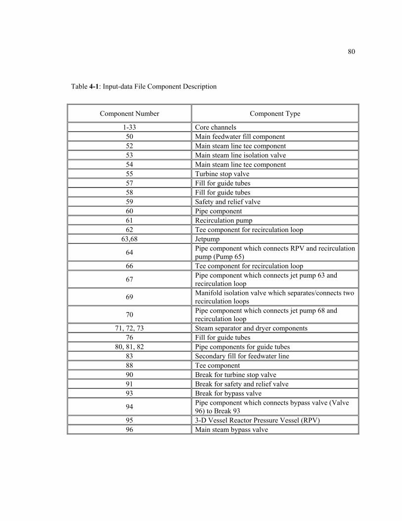
80
Component Number Component Type
1-33 Core channels 50 Main feedwater fill component 52 Main steam line tee component 53 Main steam line isolation valve 54 Main steam line tee component 55 Turbine stop valve 57 Fill for guide tubes 58 Fill for guide tubes 59 Safety and relief valve 60 Pipe component 61 Recirculation pump 62 Tee component for recirculation loop
63,68 Jetpump
64 Pipe component which connects RPV and recirculation pump (Pump 65)
66 Tee component for recirculation loop
67 Pipe component which connects jet pump 63 and recirculation loop
69 Manifold isolation valve which separates/connects two recirculation loops
70 Pipe component which connects jet pump 68 and recirculation loop
71, 72, 73 Steam separator and dryer components 76 Fill for guide tubes
80, 81, 82 Pipe components for guide tubes 83 Secondary fill for feedwater line 88 Tee component 90 Break for turbine stop valve 91 Break for safety and relief valve 93 Break for bypass valve
94 Pipe component which connects bypass valve (Valve 96) to Break 93
95 3-D Vessel Reactor Pressure Vessel (RPV) 96 Main steam bypass valve
Table 4-1: Input-data File Component Description
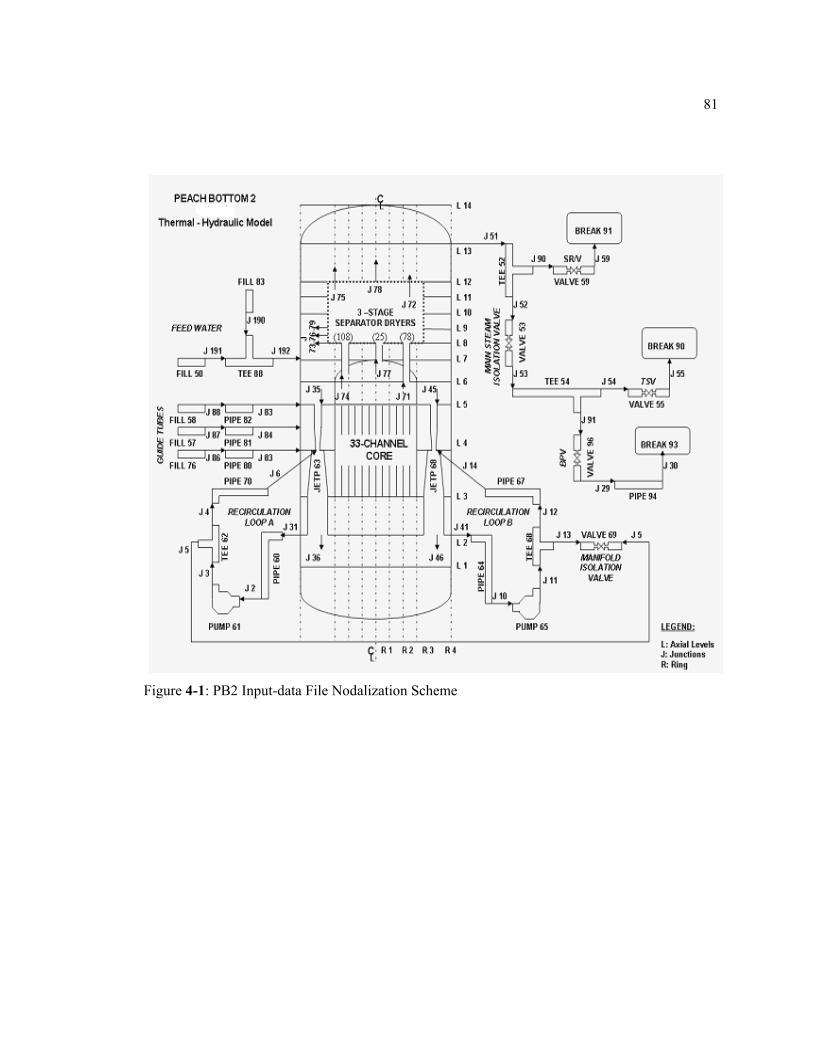
81
Figure 4-1: PB2 Input-data File Nodalization Scheme

82
4.2 PARCS Neutronics Model
A PARCS neutronics model was developed for PB2 based on the end-of cycle state core
conditions. The core is a BWR/4 consisting of 764 fuel assemblies and 185 control rods and at the
time of the TT2 test there were 576 7x7 and 188 8x8 fuel assembly type. The PARCS model
represents each of the 764 fuel assemblies as a single neutronics node. The active core height of
PB2 is 365 cm and is modeled in PARCS with 24 axial layers. At the top and bottom of the active
core the PARCS model uses additional 15.24 cm thick axial reflector regions. As noted
previously, asymmetries in the radial burnup distribution result in an asymmetric which requires
the use of full core model.
The benchmark specifications [17] provide a cross-section library with 432 sets of cross
sections in the fuel region and 3 sets for the reflector region (bottom, top, and radial reflector).
The group constants for each set consists of two types of macroscopic cross section data, one for
rodded and one for unrodded fuel assemblies. The Peach Bottom Unit 2 core is equipped with
LPRMs and forty-three detector strings are provided for the in-core instrumentation with each
string containing four LPRM located at four axial elevations in the core. In the cross section
library, the microscopic fission cross sections are provided for fissile material of the fission
chambers, as well as the assembly detector factors which are the ratio between the flux in the
detector location and the average flux in the neutronic cell. An LPRM model was developed and
implemented in PARCS in order to compare the calculations with the measured in-core detector
signals.
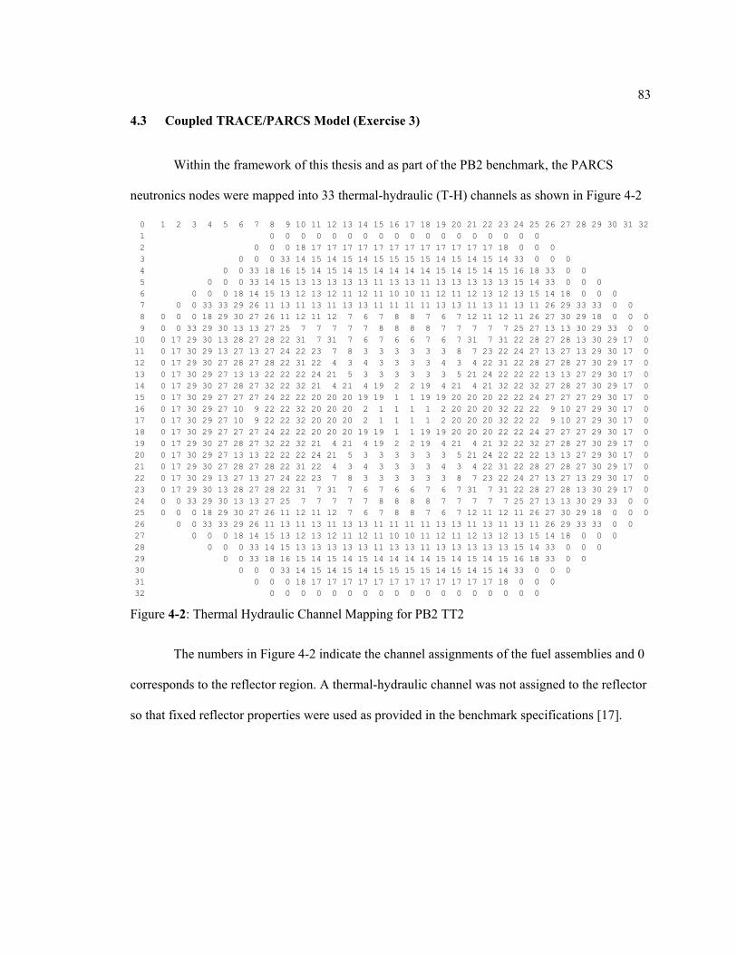
83
4.3 Coupled TRACE/PARCS Model (Exercise 3)
Within the framework of this thesis and as part of the PB2 benchmark, the PARCS
neutronics nodes were mapped into 33 thermal-hydraulic (T-H) channels as shown in Figure 4-2
The numbers in Figure 4-2 indicate the channel assignments of the fuel assemblies and 0
corresponds to the reflector region. A thermal-hydraulic channel was not assigned to the reflector
so that fixed reflector properties were used as provided in the benchmark specifications [17].
0 1 2 3 4 5 6 7 8 9 10 11 12 13 14 15 16 17 18 19 20 21 22 23 24 25 26 27 28 29 30 31 32 1 0 0 0 0 0 0 0 0 0 0 0 0 0 0 0 0 0 0 2 0 0 0 18 17 17 17 17 17 17 17 17 17 17 17 17 18 0 0 0 3 0 0 0 33 14 15 14 15 14 15 15 15 15 14 15 14 15 14 33 0 0 0 4 0 0 33 18 16 15 14 15 14 15 14 14 14 14 15 14 15 14 15 16 18 33 0 0 5 0 0 0 33 14 15 13 13 13 13 13 11 13 13 11 13 13 13 13 13 15 14 33 0 0 0 6 0 0 0 18 14 15 13 12 13 12 11 12 11 10 10 11 12 11 12 13 12 13 15 14 18 0 0 0 7 0 0 33 33 29 26 11 13 11 13 11 13 13 11 11 11 11 13 13 11 13 11 13 11 26 29 33 33 0 0 8 0 0 0 18 29 30 27 26 11 12 11 12 7 6 7 8 8 7 6 7 12 11 12 11 26 27 30 29 18 0 0 0 9 0 0 33 29 30 13 13 27 25 7 7 7 7 7 8 8 8 8 7 7 7 7 7 25 27 13 13 30 29 33 0 0 10 0 17 29 30 13 28 27 28 22 31 7 31 7 6 7 6 6 7 6 7 31 7 31 22 28 27 28 13 30 29 17 0 11 0 17 30 29 13 27 13 27 24 22 23 7 8 3 3 3 3 3 3 8 7 23 22 24 27 13 27 13 29 30 17 0 12 0 17 29 30 27 28 27 28 22 31 22 4 3 4 3 3 3 3 4 3 4 22 31 22 28 27 28 27 30 29 17 0 13 0 17 30 29 27 13 13 22 22 22 24 21 5 3 3 3 3 3 3 5 21 24 22 22 22 13 13 27 29 30 17 0 14 0 17 29 30 27 28 27 32 22 32 21 4 21 4 19 2 2 19 4 21 4 21 32 22 32 27 28 27 30 29 17 0 15 0 17 30 29 27 27 27 24 22 22 20 20 20 19 19 1 1 19 19 20 20 20 22 22 24 27 27 27 29 30 17 0 16 0 17 30 29 27 10 9 22 22 32 20 20 20 2 1 1 1 1 2 20 20 20 32 22 22 9 10 27 29 30 17 0 17 0 17 30 29 27 10 9 22 22 32 20 20 20 2 1 1 1 1 2 20 20 20 32 22 22 9 10 27 29 30 17 0 18 0 17 30 29 27 27 27 24 22 22 20 20 20 19 19 1 1 19 19 20 20 20 22 22 24 27 27 27 29 30 17 0 19 0 17 29 30 27 28 27 32 22 32 21 4 21 4 19 2 2 19 4 21 4 21 32 22 32 27 28 27 30 29 17 0 20 0 17 30 29 27 13 13 22 22 22 24 21 5 3 3 3 3 3 3 5 21 24 22 22 22 13 13 27 29 30 17 0 21 0 17 29 30 27 28 27 28 22 31 22 4 3 4 3 3 3 3 4 3 4 22 31 22 28 27 28 27 30 29 17 0 22 0 17 30 29 13 27 13 27 24 22 23 7 8 3 3 3 3 3 3 8 7 23 22 24 27 13 27 13 29 30 17 0 23 0 17 29 30 13 28 27 28 22 31 7 31 7 6 7 6 6 7 6 7 31 7 31 22 28 27 28 13 30 29 17 0 24 0 0 33 29 30 13 13 27 25 7 7 7 7 7 8 8 8 8 7 7 7 7 7 25 27 13 13 30 29 33 0 0 25 0 0 0 18 29 30 27 26 11 12 11 12 7 6 7 8 8 7 6 7 12 11 12 11 26 27 30 29 18 0 0 0 26 0 0 33 33 29 26 11 13 11 13 11 13 13 11 11 11 11 13 13 11 13 11 13 11 26 29 33 33 0 0 27 0 0 0 18 14 15 13 12 13 12 11 12 11 10 10 11 12 11 12 13 12 13 15 14 18 0 0 0 28 0 0 0 33 14 15 13 13 13 13 13 11 13 13 11 13 13 13 13 13 15 14 33 0 0 0 29 0 0 33 18 16 15 14 15 14 15 14 14 14 14 15 14 15 14 15 16 18 33 0 0 30 0 0 0 33 14 15 14 15 14 15 15 15 15 14 15 14 15 14 33 0 0 0 31 0 0 0 18 17 17 17 17 17 17 17 17 17 17 17 17 18 0 0 0 32 0 0 0 0 0 0 0 0 0 0 0 0 0 0 0 0 0 0
Figure 4-2: Thermal Hydraulic Channel Mapping for PB2 TT2

84
4.4 PB2 TT2 Steady State Results
Correct modeling of the initial steady state is important. The TT2 test has been initiated
from the steady state conditions of the EOC2.
4.4.1 Steady State Stand Alone Results (Exercise 1)
A comparison of the TRACE predictions for Exercise 1 with the plant data is shown in
Table 4-3. In Figure 4.3 the core average axial void fraction predicted by TRACE is compared
with the code used by Exelon for core analysis, RETRAN. As indicated, the TRACE results are
in excellent agreement with the steady state parameters. The maximum deviation for the core
inlet sub-cooling is less than 0.7%. The inlet sub-cooling usually depends on the amount of steam
carry-under from the separator. The transient response of the system is very sensitive to separator
modeling because this affects the initial location of the bulk boiling in core channels. The
accuracy of the core pressure drop is affected mostly by the loss coefficients in the vessel and
channels. The loss coefficients are defined through series of sensitivity studies.
The most challenging part of the steady state analysis is the prediction of the void
fraction distribution. This prediction depends on the modeling of core channels, vessel levels,
steam dryers/separators, jet pumps and recirculation loops and also depends on the features of the
TRACE code such as heat transfer models and sub-cooled boiling model.
The transient response of the system is very sensitive to the separator modeling because
this affects the initial location of the bulk boiling in the core channels and the accuracy of the
void distribution in the core. As indicated in Figure 4.2 there is less than 1% difference in the core
average void distribution and excellent agreement in the prediction of the axial void distribution
to the RETRAN code.
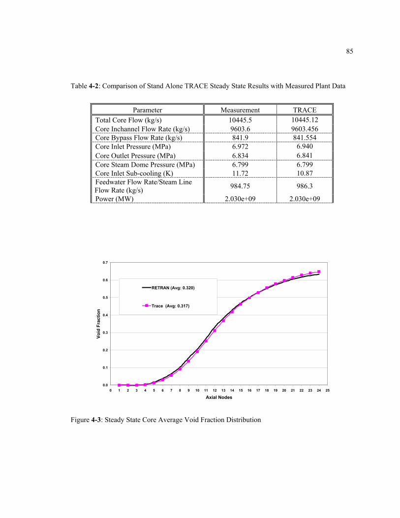
85
Parameter Measurement TRACE Total Core Flow (kg/s) 10445.5 10445.12 Core Inchannel Flow Rate (kg/s) 9603.6 9603.456 Core Bypass Flow Rate (kg/s) 841.9 841.554 Core Inlet Pressure (MPa) 6.972 6.940 Core Outlet Pressure (MPa) 6.834 6.841 Core Steam Dome Pressure (MPa) 6.799 6.799 Core Inlet Sub-cooling (K) 11.72 10.87 Feedwater Flow Rate/Steam Line Flow Rate (kg/s) 984.75 986.3
Power (MW) 2.030e+09 2.030e+09
Table 4-2: Comparison of Stand Alone TRACE Steady State Results with Measured Plant Data
0.0
0.1
0.2
0.3
0.4
0.5
0.6
0.7
0 1 2 3 4 5 6 7 8 9 10 11 12 13 14 15 16 17 18 19 20 21 22 23 24 25
Axial Nodes
Void
Fra
ctio
n
RETRAN (Avg: 0.320)
Trace (Avg: 0.317)
Figure 4-3: Steady State Core Average Void Fraction Distribution
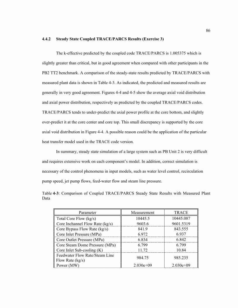
86
4.4.2 Steady State Coupled TRACE/PARCS Results (Exercise 3)
The k-effective predicted by the coupled code TRACE/PARCS is 1.005375 which is
slightly greater than critical, but in good agreement when compared with other participants in the
PB2 TT2 benchmark. A comparison of the steady-state results predicted by TRACE/PARCS with
measured plant data is shown in Table 4-3. As indicated, the predicted and measured results are
generally in very good agreement. Figures 4-4 and 4-5 show the average axial void distribution
and axial power distribution, respectively as predicted by the coupled TRACE/PARCS codes.
TRACE/PARCS tends to under-predict the axial power profile at the core bottom, and slightly
over-predict it at the core center and core top. This small discrepancy is supported by the core
axial void distribution in Figure 4-4. A possible reason could be the application of the particular
heat transfer model used in the TRACE code version.
In summary, steady state simulation of a large system such as PB Unit 2 is very difficult
and requires extensive work on each component’s model. In addition, correct simulation is
necessary of the control phenomena in input models, such as water level control, recirculation
pump speed, jet pump flows, feed-water flow and steam line pressure.
Parameter Measurement TRACE Total Core Flow (kg/s) 10445.5 10445.087 Core Inchannel Flow Rate (kg/s) 9603.6 9601.5319 Core Bypass Flow Rate (kg/s) 841.9 843.555 Core Inlet Pressure (MPa) 6.972 6.937 Core Outlet Pressure (MPa) 6.834 6.842 Core Steam Dome Pressure (MPa) 6.799 6.799 Core Inlet Sub-cooling (K) 11.72 10.84 Feedwater Flow Rate/Steam Line Flow Rate (kg/s) 984.75 985.235
Power (MW) 2.030e+09 2.030e+09
Table 4-3: Comparison of Coupled TRACE/PARCS Steady State Results with Measured Plant Data
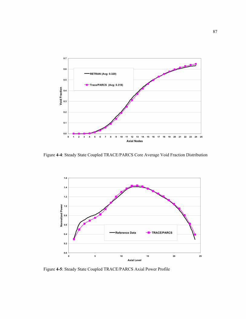
87
0.0
0.1
0.2
0.3
0.4
0.5
0.6
0.7
0 1 2 3 4 5 6 7 8 9 10 11 12 13 14 15 16 17 18 19 20 21 22 23 24 25
Axial Nodes
Void
Fra
ctio
n
RETRAN (Avg: 0.320)
Trace/PARCS (Avg: 0.318)
Figure 4-4: Steady State Coupled TRACE/PARCS Core Average Void Fraction Distribution
0.0
0.2
0.4
0.6
0.8
1.0
1.2
1.4
1.6
0 5 10 15 20 25
Axial Level
Nor
mal
ized
Pow
er
Reference Data TRACE/PARCS
Figure 4-5: Steady State Coupled TRACE/PARCS Axial Power Profile
88
4.5 PB2 TT2 Transient Results
The calculated transient results and the comparisons presented in this chapter not only
provide an opportunity to understand the phenomena behind the turbine transient tests but also to
engage in comprehensive testing and examination of the capability of TRACE/PARCS to
simulate such transient.
4.5.1 TRACE Stand Alone Transient Results (Exercise 1)
During the transient analyses of PB2 TT2 it was observed that a major impact on the
pressure response is associated with the steam bypass line together with the main steam line via
the relative position of the TSV and BPV. It was seen that the acoustical pressure wave
(oscillation) can exist in the reactor main steam piping due to the combined compressibility and
momentum effects in the steam line. The fundamental mode of the acoustical pressure oscillation
is strongly excited as a result of the turbine trip, which causes a sharp initial pressure rise in the
reactor as the first pressure wave enters the reactor vessel. In addition, the fundamental acoustical
mode propagates in the main steam piping, entering the reactor vessel and passing through the
steam separators into the reactor core with relatively little attenuation. These physical facts can be
seen in Figures 4-5 and 4-6, where the time histories for the total core mass flow rate and steam
dome pressure are shown respectively.
The time of the maximum peaks at major locations is compared to the measured plant
data in Table 4-4
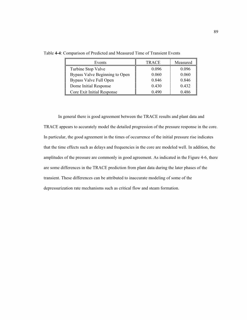
89
In general there is good agreement between the TRACE results and plant data and
TRACE appears to accurately model the detailed progression of the pressure response in the core.
In particular, the good agreement in the times of occurrence of the initial pressure rise indicates
that the time effects such as delays and frequencies in the core are modeled well. In addition, the
amplitudes of the pressure are commonly in good agreement. As indicated in the Figure 4-6, there
are some differences in the TRACE prediction from plant data during the later phases of the
transient. These differences can be attributed to inaccurate modeling of some of the
depressurization rate mechanisms such as critical flow and steam formation.
Table 4-4: Comparison of Predicted and Measured Time of Transient Events
Events TRACE Measured Turbine Stop Valve 0.096 0.096 Bypass Valve Beginning to Open 0.060 0.060 Bypass Valve Full Open 0.846 0.846 Dome Initial Response 0.430 0.432 Core Exit Initial Response 0.490 0.486
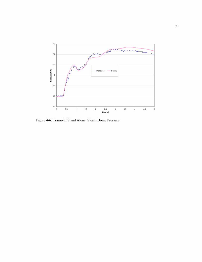
90
6.7
6.8
6.9
7
7.1
7.2
7.3
0 0.5 1 1.5 2 2.5 3 3.5 4 4.5 5
Time [s]
Pres
sure
[MPa
]
Measured TRACE
Figure 4-6: Transient Stand Alone Steam Dome Pressure
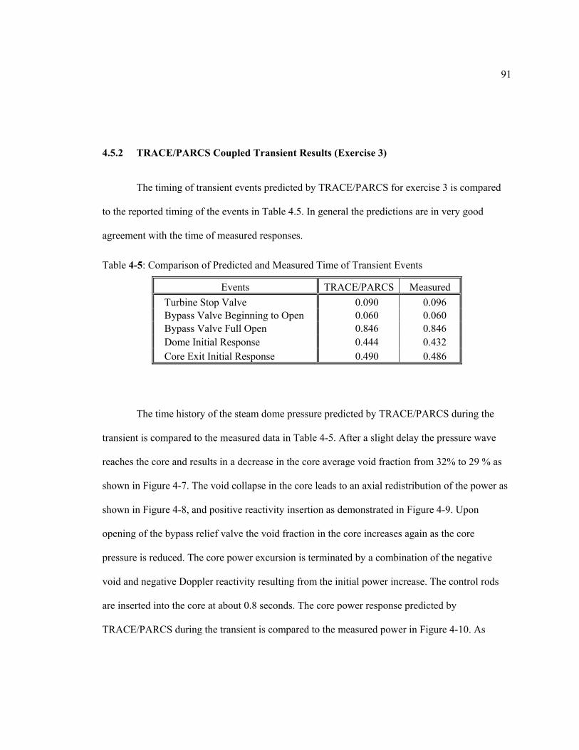
91
4.5.2 TRACE/PARCS Coupled Transient Results (Exercise 3)
The timing of transient events predicted by TRACE/PARCS for exercise 3 is compared
to the reported timing of the events in Table 4.5. In general the predictions are in very good
agreement with the time of measured responses.
The time history of the steam dome pressure predicted by TRACE/PARCS during the
transient is compared to the measured data in Table 4-5. After a slight delay the pressure wave
reaches the core and results in a decrease in the core average void fraction from 32% to 29 % as
shown in Figure 4-7. The void collapse in the core leads to an axial redistribution of the power as
shown in Figure 4-8, and positive reactivity insertion as demonstrated in Figure 4-9. Upon
opening of the bypass relief valve the void fraction in the core increases again as the core
pressure is reduced. The core power excursion is terminated by a combination of the negative
void and negative Doppler reactivity resulting from the initial power increase. The control rods
are inserted into the core at about 0.8 seconds. The core power response predicted by
TRACE/PARCS during the transient is compared to the measured power in Figure 4-10. As
Table 4-5: Comparison of Predicted and Measured Time of Transient Events
Events TRACE/PARCS Measured Turbine Stop Valve 0.090 0.096 Bypass Valve Beginning to Open 0.060 0.060 Bypass Valve Full Open 0.846 0.846 Dome Initial Response 0.444 0.432 Core Exit Initial Response 0.490 0.486
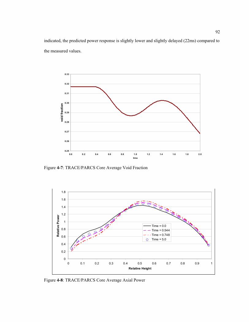
92
indicated, the predicted power response is slightly lower and slightly delayed (22ms) compared to
the measured values.
0.25
0.26
0.27
0.28
0.29
0.30
0.31
0.32
0.33
0.0 0.2 0.4 0.6 0.8 1.0 1.2 1.4 1.6 1.8 2.0
time
void
frac
tion
Figure 4-7: TRACE/PARCS Core Average Void Fraction
0
0.2
0.4
0.6
0.8
1
1.2
1.4
1.6
1.8
0 0.1 0.2 0.3 0.4 0.5 0.6 0.7 0.8 0.9 1Relative Height
Rel
ativ
e Po
wer
Time = 0.0Time = 0.544Time = 0.748Time = 5.0
Figure 4-8: TRACE/PARCS Core Average Axial Power
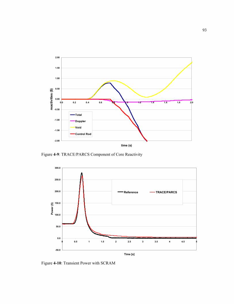
93
-50.0
0.0
50.0
100.0
150.0
200.0
250.0
300.0
0 0.5 1 1.5 2 2.5 3 3.5 4 4.5 5
Time [s]
Pow
er (5
)
Reference TRACE/PARCS
Figure 4-10: Transient Power with SCRAM
-2.00
-1.50
-1.00
-0.50
0.00
0.50
1.00
1.50
2.00
0.0 0.2 0.4 0.6 0.8 1.0 1.2 1.4 1.6 1.8 2.0
time (s)
reac
tiviti
es ($
)
Total
Doppler
Void
Control Rod
Figure 4-9: TRACE/PARCS Component of Core Reactivity
94
Chapter 5
TRACE/PARCS PB Low Flow Stability Results
Chapter 5 focuses on the LFS simulation results and their discussion. At first the steady
state results are shown and compared with available measured data. This is important in order to
demonstrate that a steady state consistent with the actual plant data was achieved. Follows the
transient results where stability parameters from time series generated in the transient calculations
are presented and discussed. The PB2 TRACE/PARCS model used here was the same as used
previously for the PB2 TT2 analyses. The stability simulation calculation begins with a stand-
alone TRACE initialization of the thermal-hydraulics field using a fixed power distribution. Upon
convergence a steady state calculation is then performed with the coupled TRACE/PARCS code
to achieve a converged coupled thermal-hydraulic/neutron flux solution. Only coupled simulation
results are shown here.
5.1 PB2 Low Flow Stability Tests Steady State Results
The list of parameters chosen for comparison covers reactor power, core mass flow rate,
steam dome pressure, core inlet temperature, core inlet sub-cooling, core average axial power
distribution and feed-water mass flow rate. The steady state results for points PT1, PT2 and PT3
are each point are shown in Tables 5-1, 5-2 and 5-3, respectively. It should be noted that there is a
good agreement among all the parameters when compared to the reference data. The feed-water
mass flow rate for each test point is slightly higher which suggest that the controller for inlet sub-
cooling needs further investigation. In order to confirm that coupled steady state was reached the
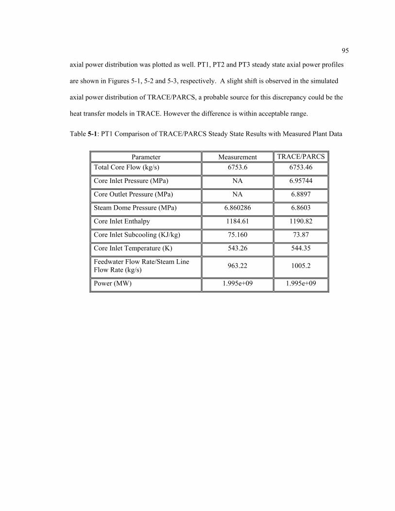
95
axial power distribution was plotted as well. PT1, PT2 and PT3 steady state axial power profiles
are shown in Figures 5-1, 5-2 and 5-3, respectively. A slight shift is observed in the simulated
axial power distribution of TRACE/PARCS, a probable source for this discrepancy could be the
heat transfer models in TRACE. However the difference is within acceptable range.
Parameter Measurement TRACE/PARCSTotal Core Flow (kg/s) 6753.6 6753.46
Core Inlet Pressure (MPa) NA 6.95744
Core Outlet Pressure (MPa) NA 6.8897
Steam Dome Pressure (MPa) 6.860286 6.8603
Core Inlet Enthalpy 1184.61 1190.82
Core Inlet Subcooling (KJ/kg) 75.160 73.87
Core Inlet Temperature (K) 543.26 544.35
Feedwater Flow Rate/Steam Line Flow Rate (kg/s) 963.22 1005.2
Power (MW) 1.995e+09 1.995e+09
Table 5-1: PT1 Comparison of TRACE/PARCS Steady State Results with Measured Plant Data
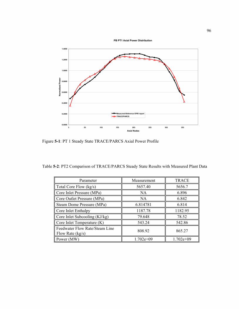
96
Parameter Measurement TRACE Total Core Flow (kg/s) 5657.40 5656.7 Core Inlet Pressure (MPa) NA 6.896 Core Outlet Pressure (MPa) NA 6.842 Steam Dome Pressure (MPa) 6.814781 6.814 Core Inlet Enthalpy 1187.78 1182.95 Core Inlet Subcooling (KJ/kg) 79.648 78.52 Core Inlet Temperature (K) 543.24 542.86 Feedwater Flow Rate/Steam Line Flow Rate (kg/s) 808.92 865.27
Power (MW) 1.702e+09 1.702e+09
PB PT1 Axial Power Distribution
0.0000
0.2000
0.4000
0.6000
0.8000
1.0000
1.2000
1.4000
3 53 103 153 203 253 303 353
Axial Nodes
Nor
mal
ized
Pow
er
Measured-Reference EPRI reportTRACE/PARCS
Figure 5-1: PT 1 Steady State TRACE/PARCS Axial Power Profile
Table 5-2: PT2 Comparison of TRACE/PARCS Steady State Results with Measured Plant Data
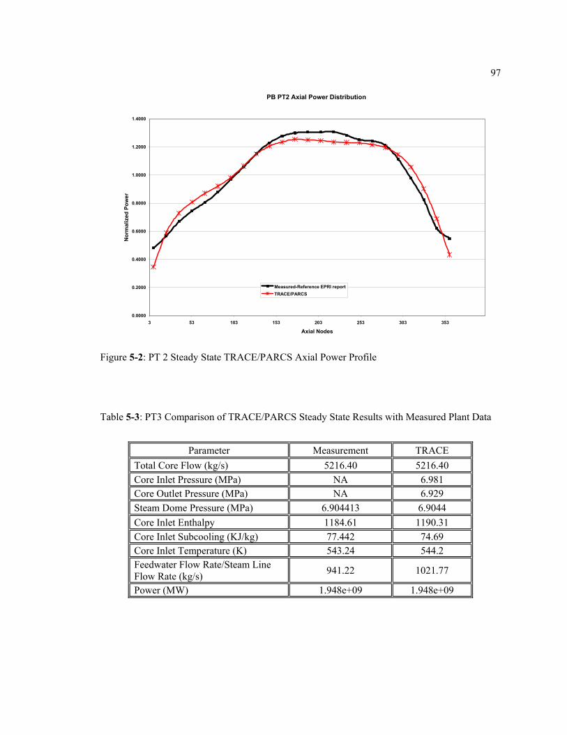
97
Parameter Measurement TRACE Total Core Flow (kg/s) 5216.40 5216.40 Core Inlet Pressure (MPa) NA 6.981 Core Outlet Pressure (MPa) NA 6.929 Steam Dome Pressure (MPa) 6.904413 6.9044 Core Inlet Enthalpy 1184.61 1190.31 Core Inlet Subcooling (KJ/kg) 77.442 74.69 Core Inlet Temperature (K) 543.24 544.2 Feedwater Flow Rate/Steam Line Flow Rate (kg/s) 941.22 1021.77
Power (MW) 1.948e+09 1.948e+09
PB PT2 Axial Power Distribution
0.0000
0.2000
0.4000
0.6000
0.8000
1.0000
1.2000
1.4000
3 53 103 153 203 253 303 353
Axial Nodes
Nor
mal
ized
Pow
er
Measured-Reference EPRI reportTRACE/PARCS
Figure 5-2: PT 2 Steady State TRACE/PARCS Axial Power Profile
Table 5-3: PT3 Comparison of TRACE/PARCS Steady State Results with Measured Plant Data
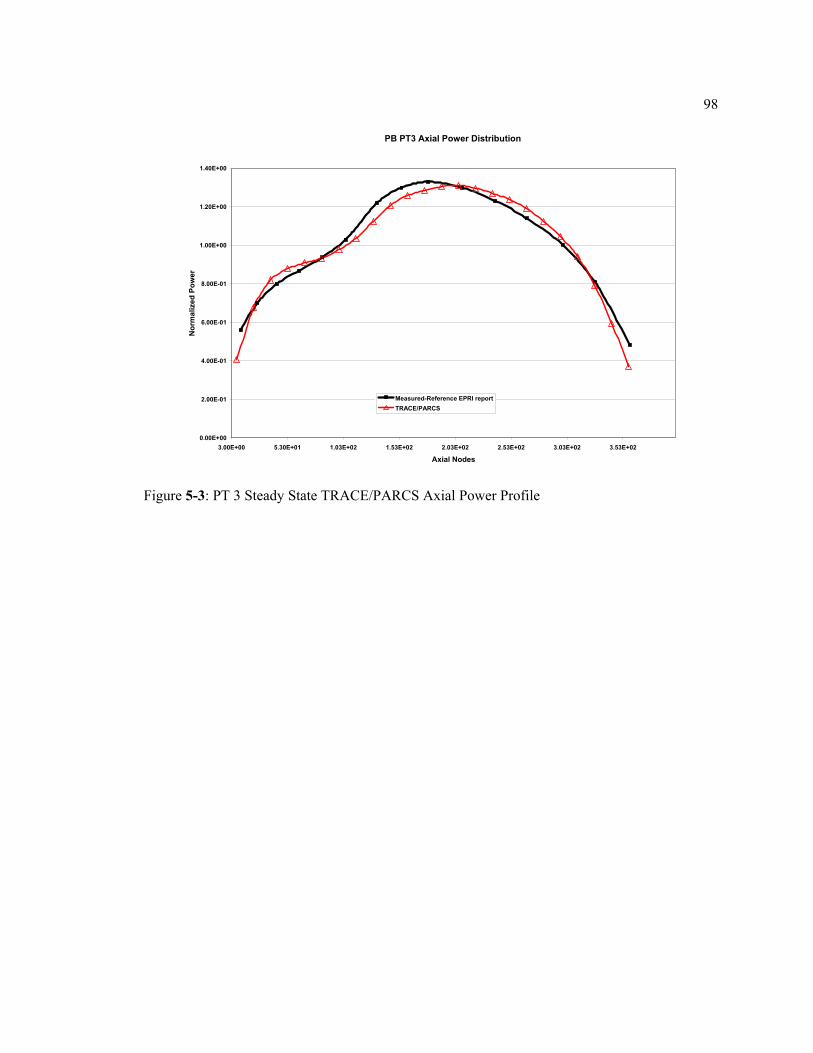
98
PB PT3 Axial Power Distribution
0.00E+00
2.00E-01
4.00E-01
6.00E-01
8.00E-01
1.00E+00
1.20E+00
1.40E+00
3.00E+00 5.30E+01 1.03E+02 1.53E+02 2.03E+02 2.53E+02 3.03E+02 3.53E+02
Axial Nodes
Nor
mal
ized
Pow
er
Measured-Reference EPRI reportTRACE/PARCS
Figure 5-3: PT 3 Steady State TRACE/PARCS Axial Power Profile
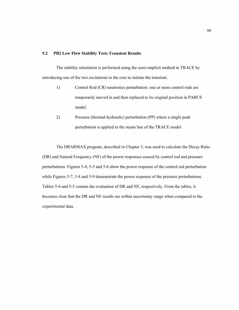
99
5.2 PB2 Low Flow Stability Tests Transient Results
The stability simulation is performed using the semi-implicit method in TRACE by
introducing one of the two excitations to the core to initiate the transient.
1) Control Rod (CR) neutronics perturbation: one or more control rods are
temporarily moved in and then replaced to its original position in PARCS
model.
2) Pressure (thermal-hydraulic) perturbation (PP) where a single peak
perturbation is applied to the steam line of the TRACE model
The DRARMAX program, described in Chapter 3, was used to calculate the Decay Ratio
(DR) and Natural Frequency (NF) of the power responses caused by control rod and pressure
perturbations. Figures 5-4, 5-5 and 5-6 show the power response of the control rod perturbation
while Figures 5-7, 5-8 and 5-9 demonstrate the power response of the pressure perturbations.
Tables 5-4 and 5-5 contain the evaluation of DR and NF, respectively. From the tables, it
becomes clear that the DR and NF results are within uncertainty range when compared to the
experimental data.
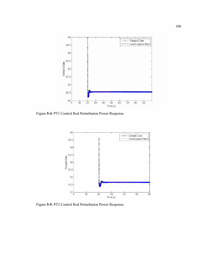
100
Figure 5-4: PT1 Control Rod Perturbation Power Response
Figure 5-5: PT2 Control Rod Perturbation Power Response
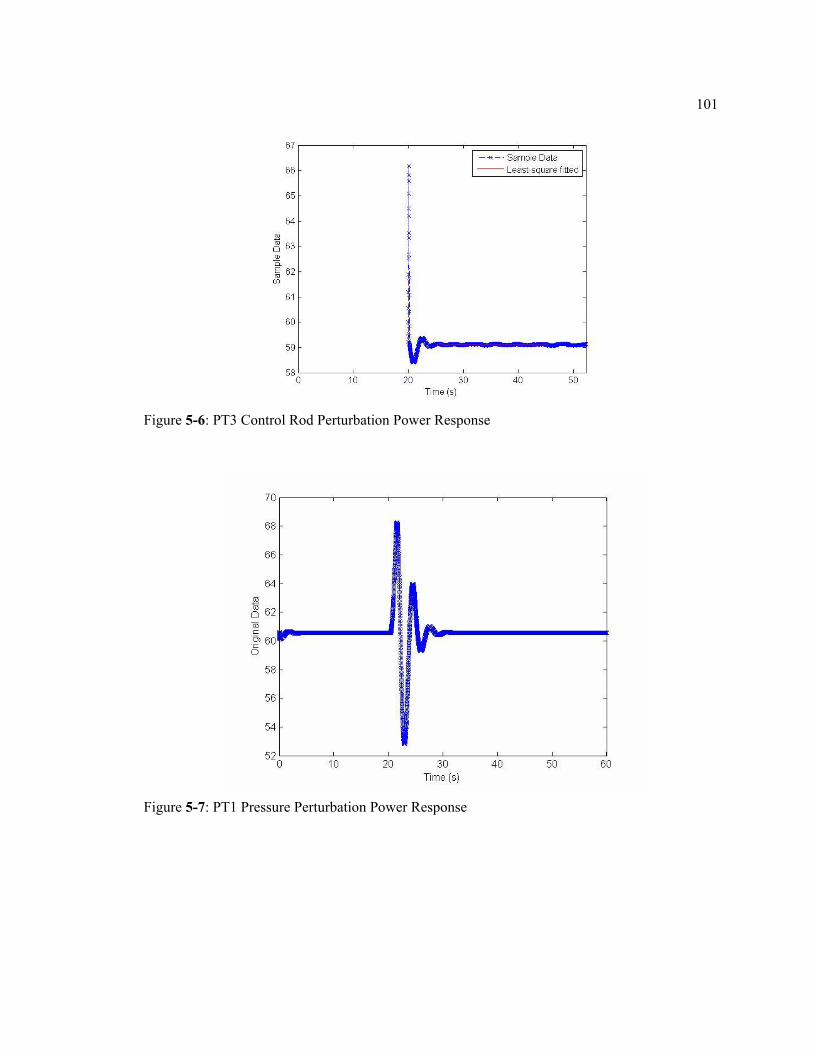
101
Figure 5-6: PT3 Control Rod Perturbation Power Response
Figure 5-7: PT1 Pressure Perturbation Power Response
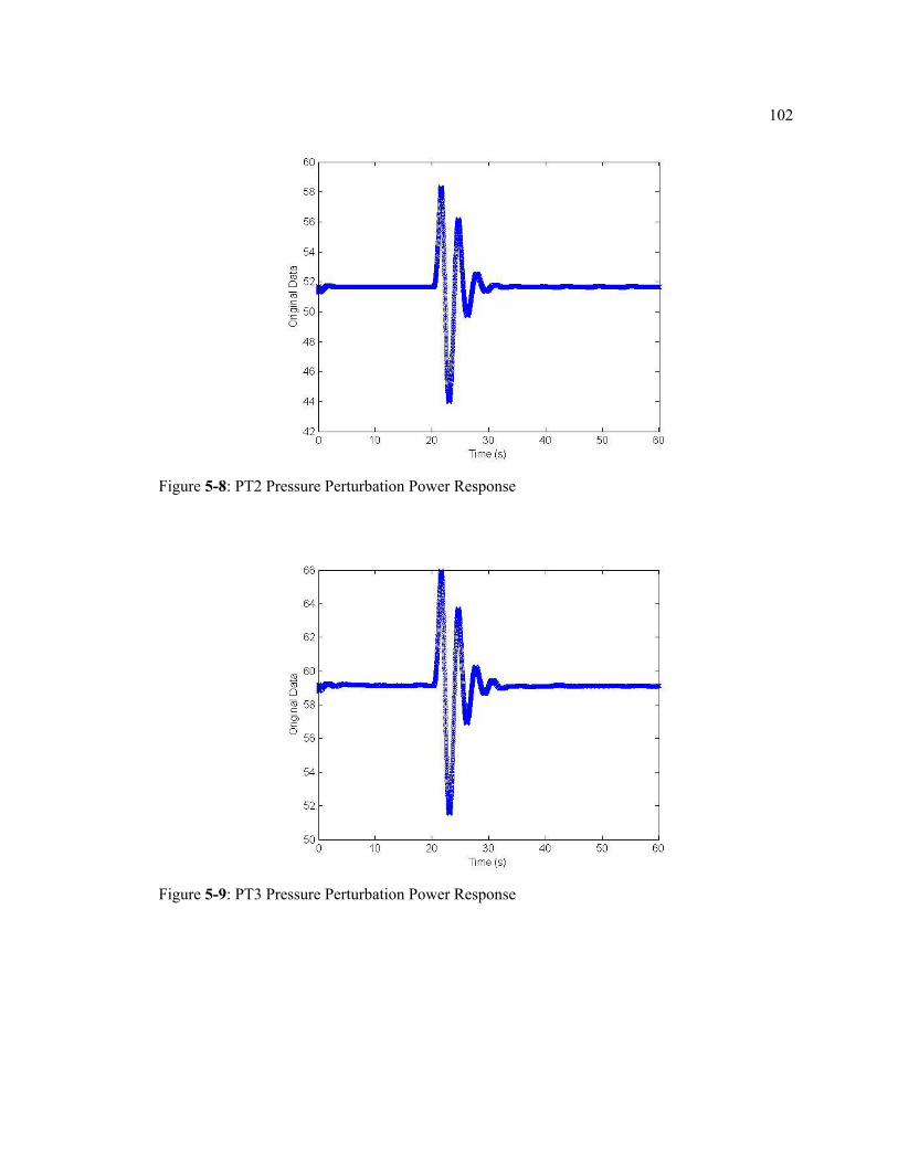
102
Figure 5-8: PT2 Pressure Perturbation Power Response
Figure 5-9: PT3 Pressure Perturbation Power Response
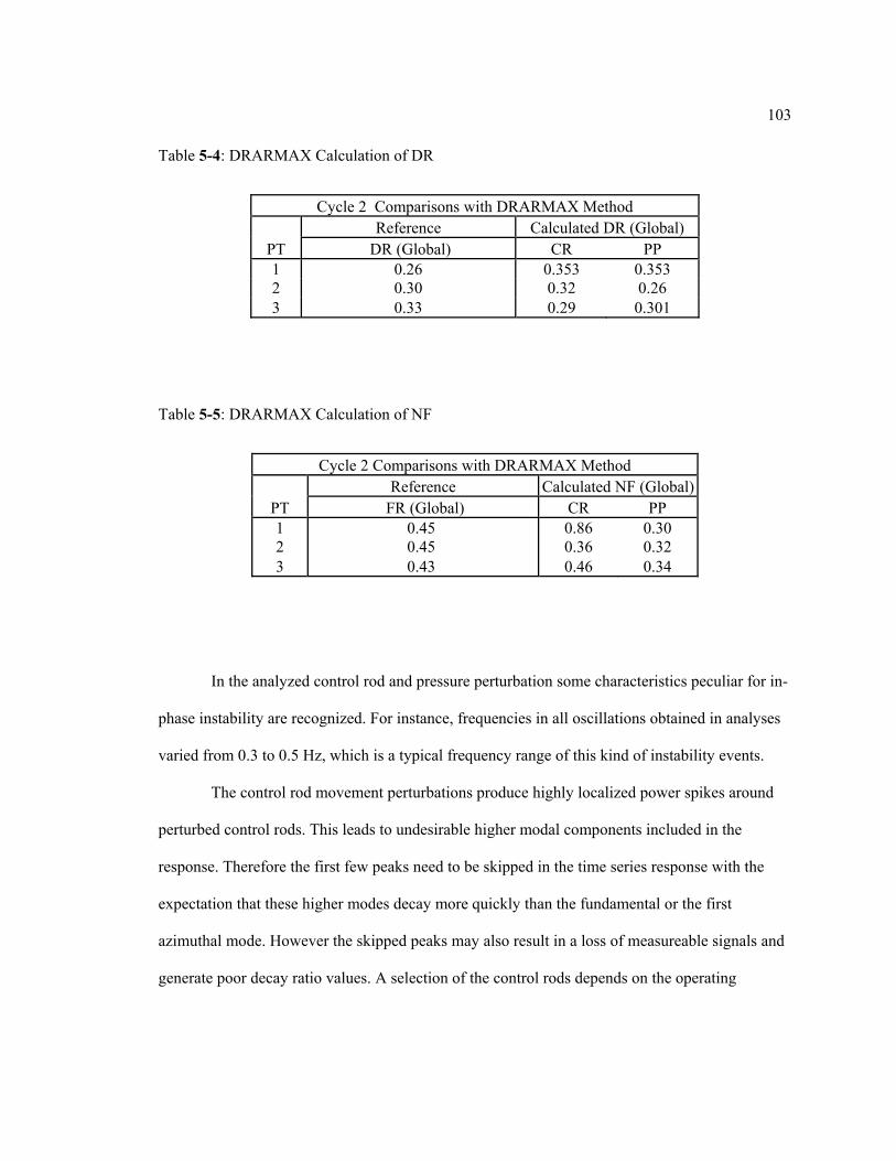
103
Cycle 2 Comparisons with DRARMAX Method Reference Calculated DR (Global)
PT DR (Global) CR PP 1 0.26 0.353 0.353 2 0.30 0.32 0.26 3 0.33 0.29 0.301
Cycle 2 Comparisons with DRARMAX Method Reference Calculated NF (Global)
PT FR (Global) CR PP 1 0.45 0.86 0.30 2 0.45 0.36 0.32 3 0.43 0.46 0.34
In the analyzed control rod and pressure perturbation some characteristics peculiar for in-
phase instability are recognized. For instance, frequencies in all oscillations obtained in analyses
varied from 0.3 to 0.5 Hz, which is a typical frequency range of this kind of instability events.
The control rod movement perturbations produce highly localized power spikes around
perturbed control rods. This leads to undesirable higher modal components included in the
response. Therefore the first few peaks need to be skipped in the time series response with the
expectation that these higher modes decay more quickly than the fundamental or the first
azimuthal mode. However the skipped peaks may also result in a loss of measureable signals and
generate poor decay ratio values. A selection of the control rods depends on the operating
Table 5-4: DRARMAX Calculation of DR
Table 5-5: DRARMAX Calculation of NF

104
condition and its influence on the excited higher modes cannot be easily quantified. Therefore it
is difficult to ensure high accuracy for DR values calculating with such perturbation
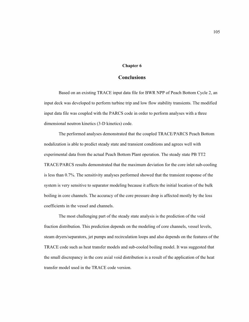
105
Chapter 6
Conclusions
Based on an existing TRACE input data file for BWR NPP of Peach Bottom Cycle 2, an
input deck was developed to perform turbine trip and low flow stability transients. The modified
input data file was coupled with the PARCS code in order to perform analyses with a three
dimensional neutron kinetics (3-D kinetics) code.
The performed analyses demonstrated that the coupled TRACE/PARCS Peach Bottom
nodalization is able to predict steady state and transient conditions and agrees well with
experimental data from the actual Peach Bottom Plant operation. The steady state PB TT2
TRACE/PARCS results demonstrated that the maximum deviation for the core inlet sub-cooling
is less than 0.7%. The sensitivity analyses performed showed that the transient response of the
system is very sensitive to separator modeling because it affects the initial location of the bulk
boiling in core channels. The accuracy of the core pressure drop is affected mostly by the loss
coefficients in the vessel and channels.
The most challenging part of the steady state analysis is the prediction of the void
fraction distribution. This prediction depends on the modeling of core channels, vessel levels,
steam dryers/separators, jet pumps and recirculation loops and also depends on the features of the
TRACE code such as heat transfer models and sub-cooled boiling model. It was suggested that
the small discrepancy in the core axial void distribution is a result of the application of the heat
transfer model used in the TRACE code version.
106
In addition, correct simulation is necessary of the control phenomena in input models,
such as water level control, recirculation pump speed, jet pump flows, feed-water flow and steam
line pressure.
During the transient analyses of PB2 TT2 it was observed that a major impact on the
pressure response has the steam bypass line together with the main steam line via the relative
position of the TSV and BPV. It was seen that the acoustical pressure wave (oscillation) can exist
in the reactor main steam piping due to the combined compressibility and momentum effects in
the steam line. TRACE appears to accurately model the detailed progression of the pressure
response in the core. There are some differences in the TRACE prediction from plant data during
the later phases of the transient. These differences can be attributed to inaccurate modeling of
some of the depressurization rate mechanisms such as critical flow and steam formation
Other transients, Low Flow Stability Tests, were simulated as well. The stability simulation
calculation begins again with steady state stand-alone and coupled calculations. During steady
state calculations, there is very good agreement among all the parameters when compared to the
reference data. A possible source of the feed-water mass flow rate discrepancies between
measured data and simulated results could be the control block which controls the inlet sub-
cooling. Another slight discrepancy was observed in the axial power distribution of
TRACE/PARCS which depends on the heat transfer models in TRACE.
After steady state validation with measured plant data, pressure and control rod
perturbation transients were performed. During transient tests it was observed that the pressure
perturbation produces better results especially in terms of natural frequency (NF), than the control
rod perturbation. This could be explained with control rod movement perturbations which
produce highly localized power spikes around perturbed control rods. This result in undesirable
higher modal components included in the response. When calculating the decay ratio (DR) and
NF the first few peaks of the power response need to be skipped with the expectation that these

107
higher modes decay more quickly than the fundamental or the first azimuthal mode. However, the
skipped peaks may also result in a loss of measureable signals and generate poor DR and NF
values and it is difficult to ensure high accuracy when simulating such perturbation.
108
REFERENCES
[1] T. Kozlowski, T. Downar, et al. Analysis of the OECD/NEA PWR Main Steam Line
Break Benchmark with TRAC-M/PACS, Nuclear Technology, September, 2004.
[2] “Transient and Stability Tests at Peach Bottom Atomic Power Station Unit 2 at End
of Cycle 2”, General Electric Company/Nuclear Energy Engineering Division, NP-564, Research
Project 1020-I, Topical Report, June 1978
[3] L. Carmichael, and R. Niemi, “Transient and Stability Tests at Peach Bottom Atomic
Power Station Unit 2 at End of Cycle 2”, EPRI NP-564, June 1978.
[4] N. Larsen, “Core Design and Operating Data for Cycles 1 and 2 of Peach Bottom 2”,
EPRI NP-563, June 1978.
[5] K. Hornyik, and J. Naser, “RETRAN Analysis of the Turbine Trip Tests at Peach
Bottom Atomic Power Station Unit 2 at the End of Cycle 2”, EPRI NP-1076-SR Special Report,
April 1979.
[6] D. Lee, T. Ulses, et al., “Analysis of the OECD/NEA Peach Bottom Turbine Trip
Benchmark with TRAC-M/PARCS,” Nuclear Science and Engineering, January, 2005.
[7] A. Olson, “Methods for Performing BWR System Transient Analysis”, Philadelphia
Electric Company, Topical Report PECo-FMS-0004-A (1988).
[8] TRACE v5.0 Theory Manual - Field Equations, Solution Methods, and Physical
Models, 15 August 2007
[9] PARCS Volume 2: User Manual for the PARCS Kinetics Core Simulator Module,
Purdue University, 15 November 2004
[10] Y. Xu 2005, DRARMAX - Users manual, 6 December 2005
[11] H. Joo, D. Barber, G. Jiang and T. Downar, “PARCS :- A Multi-Dimensional Two
Group Reactor Kinetics Code Based on the Nonlinear Analytical Nodal Method,” (1998)
109
[12] N. M. Schnurr et al. 1992, TRAC-PF1/MOD2 Theory manual, Los Alamos National
Laboratory Report LA 2031-M, US Nuclear Regulatory Commission Report NUREG/CR 5673.
[13] PARCS Volume 2: User Manual for the PARCS Kinetics Core Simulator Module,
Purdue University, 15 November 2004.
[14] S. L. Marple, 1987, “Digital Spectral Analysis with Applications”, Prentice Hall,
Englewood Cliffs, Chapter 8.
[15] J. L. Munoz, G. Verdù, C. Pereira, 1992, “Dynamic Reconstruction and Lyapunov
Exponents from Time Series Data in Boiling Water Reactor Application to BWR Stability
Analysis”, Ann. Nucl. Energy, 19, 223.
[16] F. Odar, C. Murray, R. Shumway, M. Bolander, D. Barber, J. Mahaffy - TRACE
Users Manual, 2003
[17] J. Solis, K. Ivanov, B. Sarikaya, A. Olson, and K. Hunt, “BWR TT Benchmark.
Volume I: Final Specifications”, NEA/NSC/DOC(2001)1