Towards Verifying Parallel Algorithms and Programs using …ceur-ws.org/Vol-723/paper5.pdf ·...

Towards Verifying Parallel Algorithms andPrograms using Coloured Petri Nets

Michael Westergaard

Department of Mathematics and Computer Science,Eindhoven University of Technology, The Netherlands

[email protected]

Abstract. Coloured Petri nets have proved to be a useful formalism formodeling distributed algorithms, i.e., algorithms where nodes commu-nicate via message passing. Here we describe an approach for modelingparallel algorithms and programs, i.e., algorithms and programs whereprocesses communicate via shared memory. The model is verified for cor-rectness, here to prove absence of mutual exclusion violations and to finddead- and live-locks. The approach can be used in a model-driven de-velopment approach, where code is generated from a model, in a model-extraction approach, where a model is extracted from running code, orusing a combination of the two, supporting extracting a model from anabstract description and generation of correct implementation code. Weillustrate our idea by applying the technique to a parallel implementationof explicit state-space exploration.

1 Introduction

Parallel and distributed computing address important problems of scalabilityin computer science, where some problems are too large or complex to be han-dled by just one computer. Until now, focus has mostly been on distributedalgorithms, i.e., algorithms running on multiple computers communicating via anetwork, as access to parallel computers, i.e., computers capable of running mul-tiple processes communicating via shared memory (RAM), has been limited. Forthis reason, there are many papers on modeling distributed algorithms, such asnetwork protocols [3, 5, 11, 12]. With the advance of cheap multi-core processorsand cheap multi-processor systems, access to multiple cores has become morecommon, and the development and analysis of algorithms for parallel processingbecomes very interesting. As parallel computing allows much faster communi-cation between processes, tasks that were not previously feasible or efficient todo concurrently becomes interesting. In this paper, we present our experiencesdeveloping parallel algorithms with synchronization mechanisms developed andverified by means of coloured Petri nets (CPNs) [10]. This work was motivatedby the requirement for a parallel state-space exploration algorithm. In this pa-per, we provide an approach that allows us to extract a model for analysis froma program or abstractly described algorithm in a systematic way. We do this ina way that allows us to automatically generate a skeleton implementation of the

algorithm subsequently. We use a simple state-space algorithm as example, butthe approach has also been used for other parallel algorithms, such as parts of aprotocol for operational support [16].

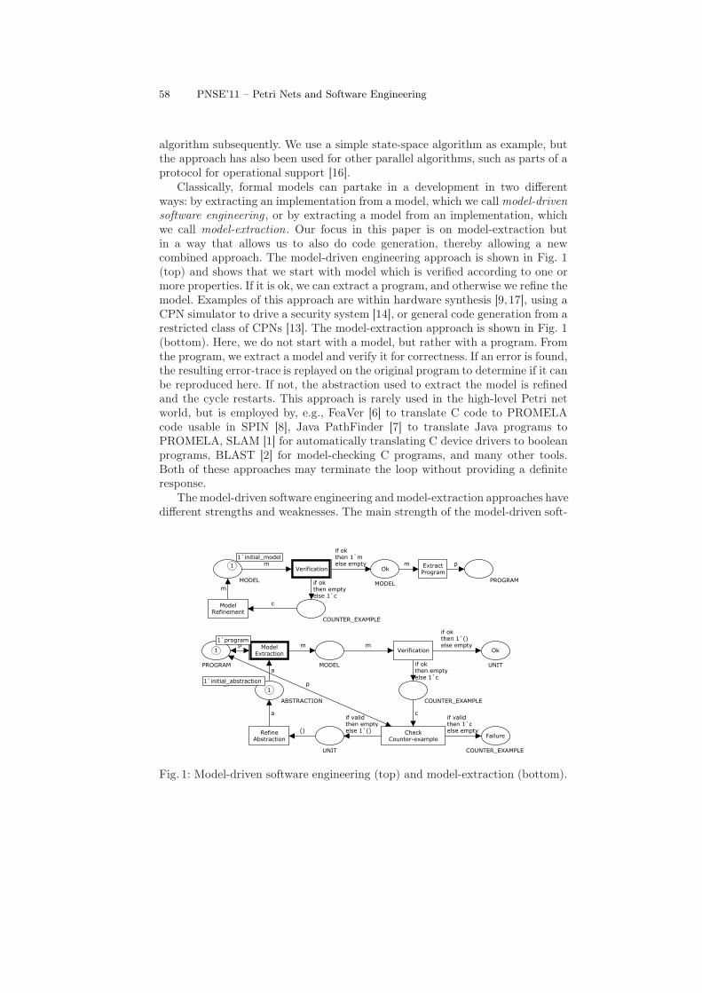
Classically, formal models can partake in a development in two differentways: by extracting an implementation from a model, which we call model-drivensoftware engineering, or by extracting a model from an implementation, whichwe call model-extraction. Our focus in this paper is on model-extraction butin a way that allows us to also do code generation, thereby allowing a newcombined approach. The model-driven engineering approach is shown in Fig. 1(top) and shows that we start with model which is verified according to one ormore properties. If it is ok, we can extract a program, and otherwise we refine themodel. Examples of this approach are within hardware synthesis [9,17], using aCPN simulator to drive a security system [14], or general code generation from arestricted class of CPNs [13]. The model-extraction approach is shown in Fig. 1(bottom). Here, we do not start with a model, but rather with a program. Fromthe program, we extract a model and verify it for correctness. If an error is found,the resulting error-trace is replayed on the original program to determine if it canbe reproduced here. If not, the abstraction used to extract the model is refinedand the cycle restarts. This approach is rarely used in the high-level Petri networld, but is employed by, e.g., FeaVer [6] to translate C code to PROMELAcode usable in SPIN [8], Java PathFinder [7] to translate Java programs toPROMELA, SLAM [1] for automatically translating C device drivers to booleanprograms, BLAST [2] for model-checking C programs, and many other tools.Both of these approaches may terminate the loop without providing a definiteresponse.

The model-driven software engineering and model-extraction approaches havedifferent strengths and weaknesses. The main strength of the model-driven soft-

m

mVerification

if okthen 1`melse empty

Ok

if okthen emptyelse 1`c

COUNTER_EXAMPLE

MODEL

ModelRefinement

MODEL

initial_model

c

ExtractProgram

m p

PROGRAM

1

1`initial_model

a

()

if validthen emptyelse 1`()

if validthen 1`celse empty

p

c


if okthen 1`()else empty

a

mmp

RefineAbstraction

CheckCounter-example

VerificationModel

Extraction

UNIT

Failure

COUNTER_EXAMPLE

COUNTER_EXAMPLE

Ok

UNIT

initial_abstraction

ABSTRACTION

MODEL

program

PROGRAM

1

1`initial_abstraction

1

1`program

Fig. 1: Model-driven software engineering (top) and model-extraction (bottom).

58 PNSE’11 – Petri Nets and Software Engineering

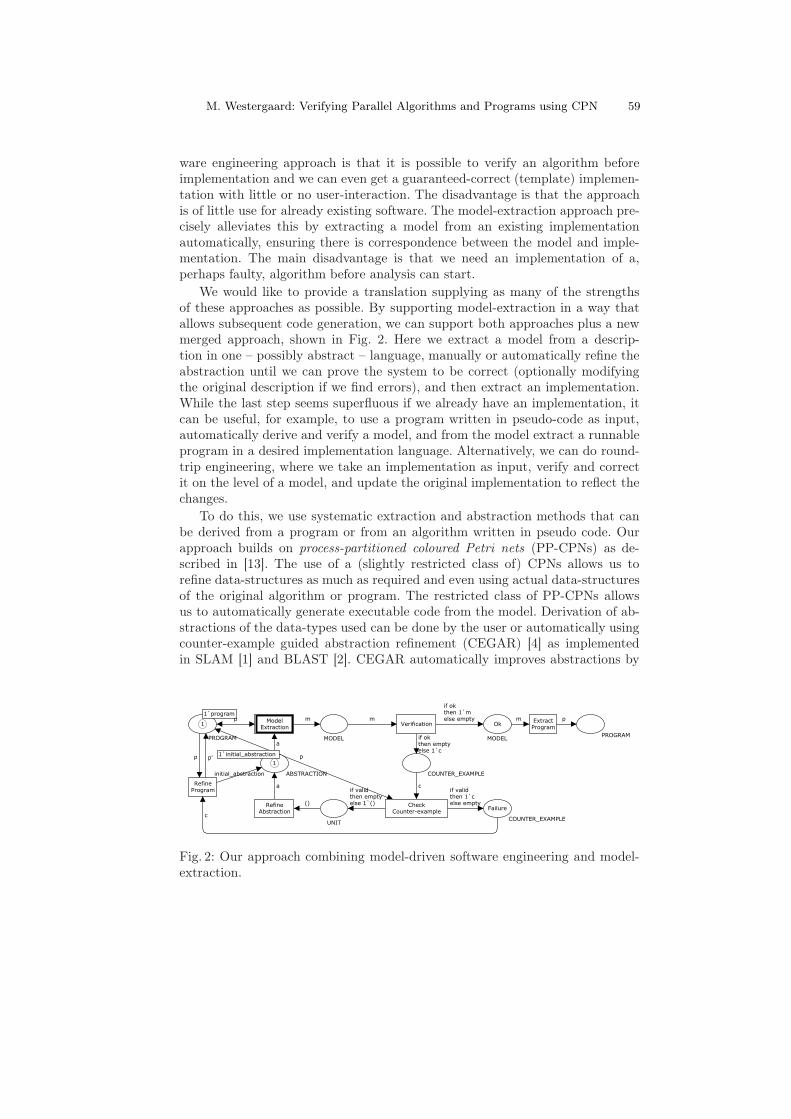
ware engineering approach is that it is possible to verify an algorithm beforeimplementation and we can even get a guaranteed-correct (template) implemen-tation with little or no user-interaction. The disadvantage is that the approachis of little use for already existing software. The model-extraction approach pre-cisely alleviates this by extracting a model from an existing implementationautomatically, ensuring there is correspondence between the model and imple-mentation. The main disadvantage is that we need an implementation of a,perhaps faulty, algorithm before analysis can start.

We would like to provide a translation supplying as many of the strengthsof these approaches as possible. By supporting model-extraction in a way thatallows subsequent code generation, we can support both approaches plus a newmerged approach, shown in Fig. 2. Here we extract a model from a descrip-tion in one – possibly abstract – language, manually or automatically refine theabstraction until we can prove the system to be correct (optionally modifyingthe original description if we find errors), and then extract an implementation.While the last step seems superfluous if we already have an implementation, itcan be useful, for example, to use a program written in pseudo-code as input,automatically derive and verify a model, and from the model extract a runnableprogram in a desired implementation language. Alternatively, we can do round-trip engineering, where we take an implementation as input, verify and correctit on the level of a model, and update the original implementation to reflect thechanges.

To do this, we use systematic extraction and abstraction methods that canbe derived from a program or from an algorithm written in pseudo code. Ourapproach builds on process-partitioned coloured Petri nets (PP-CPNs) as de-scribed in [13]. The use of a (slightly restricted class of) CPNs allows us torefine data-structures as much as required and even using actual data-structuresof the original algorithm or program. The restricted class of PP-CPNs allowsus to automatically generate executable code from the model. Derivation of ab-stractions of the data-types used can be done by the user or automatically usingcounter-example guided abstraction refinement (CEGAR) [4] as implementedin SLAM [1] and BLAST [2]. CEGAR automatically improves abstractions by

a

()

if validthen emptyelse 1`()

if validthen 1`celse empty

p

c


if okthen 1`melse empty

a

mmp

RefineAbstraction

CheckCounter-example

VerificationModel

Extraction

UNIT

Failure

COUNTER_EXAMPLE

Ok

MODEL

ABSTRACTION

MODEL

programExtractProgram

PROGRAM

pm

COUNTER_EXAMPLE

RefineProgram

c

p p'

PROGRAM

initial_abstraction

initial_abstraction

1

1`initial_abstraction

1

1`program

Fig. 2: Our approach combining model-driven software engineering and model-extraction.

M. Westergaard: Verifying Parallel Algorithms and Programs using CPN 59

replaying errors found in an abstract model on the original program and usingabout why a given error-trace cannot be replayed in the original program torefine the abstraction.

In this paper we focus on model-extraction. Our goal is to provide a proof-of-concept, so we do certain steps that can be automated by hand, such as thetranslation from code to a model using patterns. We do not address refinementafter discovery of errors in this paper, but assume an external library usingCEGAR or a user takes care of that. We have already treated the code generationaspect in [13].

The rest of this paper is structured as follows: in the next section, we in-troduce process-partitioned coloured Petri nets as defined in [13] and a simplealgorithm for state-space generation which we use as running example to illus-trate our idea. In Sect. 3, we introduce our approach to generating PP-CPNmodels from algorithms using a naive parallel version of the algorithm presentedin Sect. 2. In Sect. 4, we use state-space generation to identify a problem in theoriginal parallelization, fix the problem and show that the problem no longer ispresent in a modified version. Finally, in Sect. 5, we sum up our conclusions andprovide directions for future work.

2 Background

In this section, we briefly introduce process-partitioned CPNs as defined in [13].We also give a simple algorithm for explicit state-space generation which we useas example in the remainder of the paper.

Process-partitioned CPNs. Coloured Petri nets (CPNs) consist of places ,transitions , and arcs . Places are typed and arcs have expressions that may con-tain variables. Places may contain tokens and we call the distribution of tokenson all places a marking of the net, and the marking before executing any tran-sitions the initial marking. CPNs have a module concept, where subpages arerepresented by substitution transitions.

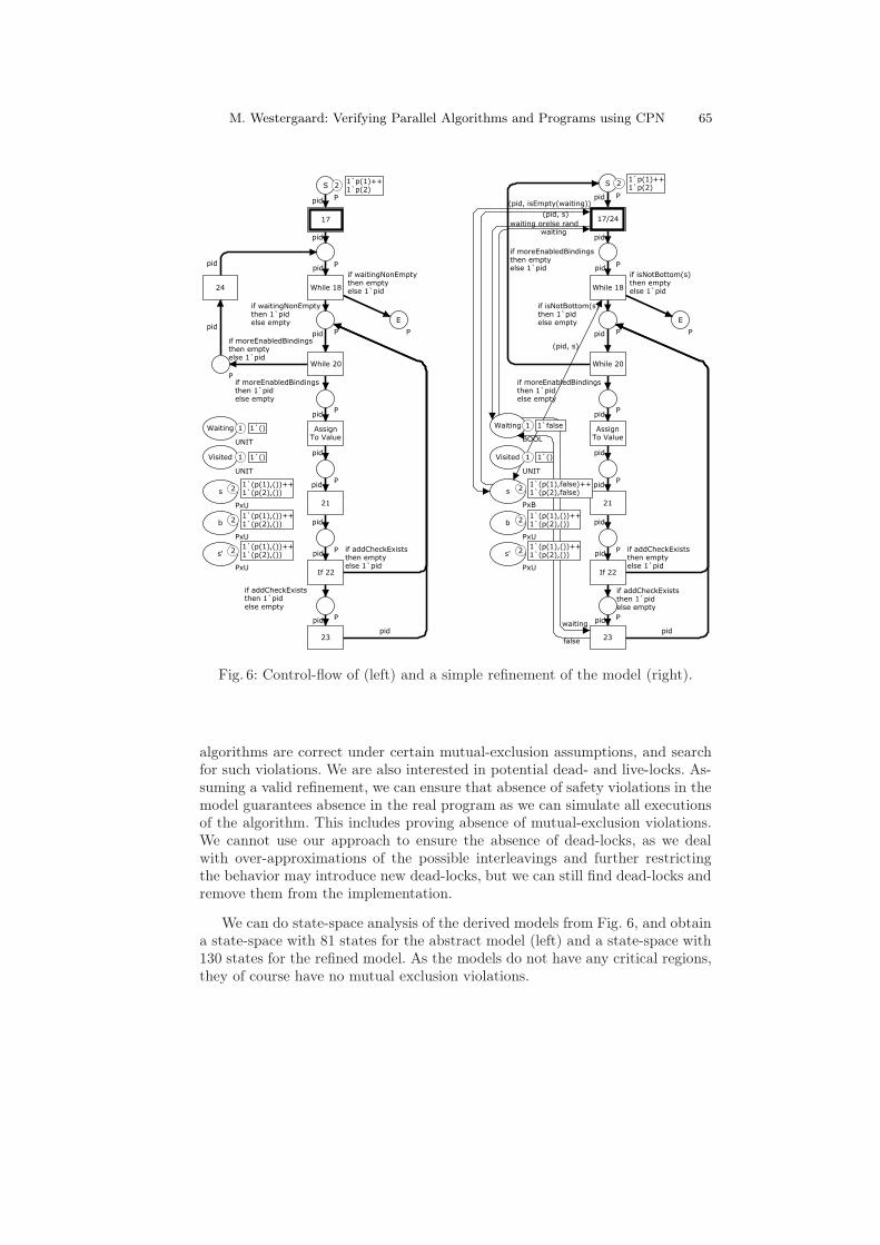
In [13] we introduce the notion of process-partitioned CPNs (PP-CPNs).These are CPNs, which are partitioned into separate kinds of processes. In thispaper, we are only interested in models containing a single kind of process, sowe just look at process subnets (Def. 2 in [13]). A single process subnet is aPP-CPN, but not necessarily the other way around, but in this paper, wheneverwe talk about PP-CPNs, we assume they consist of exactly one process subnet.A process subnet is a CPN with a distinguished process colour set serving asprocess identifier. The model in Fig. 6 (left) is an example of a PP-CPN (weprovide a detailed description of the model in Sect. 3). The process colour setof this model is P. The places of a process subnet are partitioned into processplaces , local places , and shared places (in [13], we additionally introduce bufferplaces for asynchronous communication between processes, but these are notused here). These places correspond to the control flow, the local variables, andshared variables of normal programs. Process places must have the process colour


set as type (in the example S and E and all unnamed places are process places),local places must have a product of the process colour set and any other type astype (in the example, s, b, and s’), and shared places can have any type (in theexample, Waiting and Visited).

In the initial marking, exactly one of the process places must contain alltokens of the process colour set and the remaining process places must be empty(modeling that all processes must start in the same location in the program).Local places must initially contain exactly one token for each process so that ifwe project onto the component of the process colour set, we obtain exactly onecopy of all values of the set (modeling that all local variables must be initialized).All shared places must contain exactly one value (modeling that shared variablesmust be initialized). All arc expression must ensure that tokens are preserved.

We have chosen to adopt the notion that we cannot create new processesor destroy processes from [13] even though nothing in our approach breaks ifwe allow dynamic instantiation and destruction of processes. This is mainly forsimplicity as we did not need dynamic instantiation in our examples.

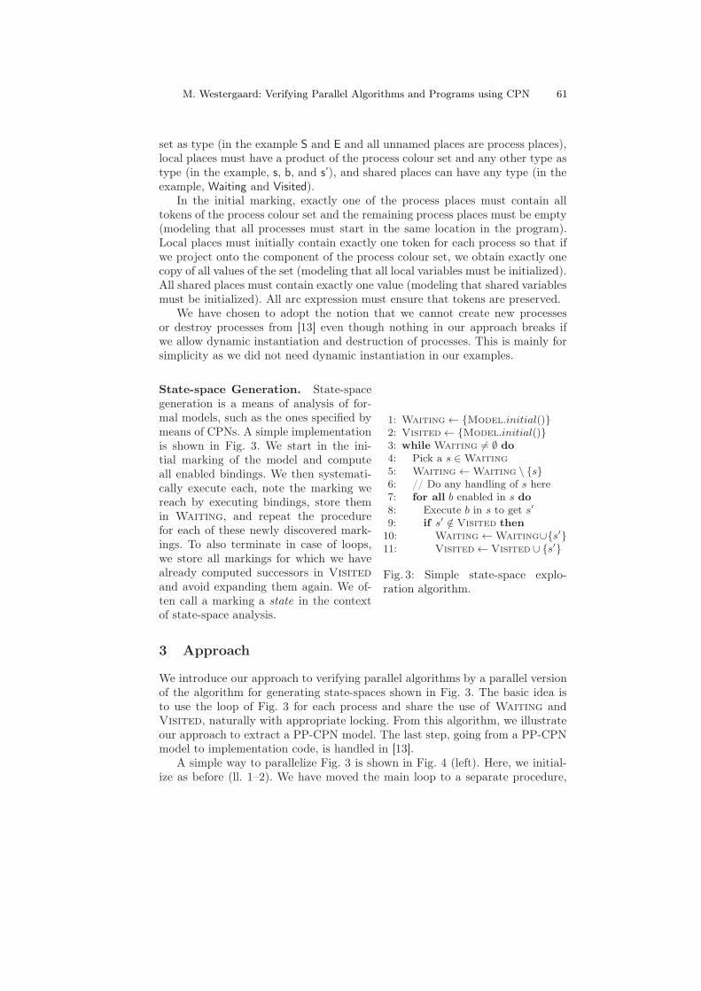
1: Waiting← {Model.initial()}2: Visited← {Model.initial()}3: while Waiting 6= ∅ do4: Pick a s ∈Waiting5: Waiting←Waiting \ {s}6: // Do any handling of s here7: for all b enabled in s do8: Execute b in s to get s′

9: if s′ /∈ Visited then10: Waiting←Waiting∪{s′}11: Visited← Visited ∪ {s′}

Fig. 3: Simple state-space explo-ration algorithm.

State-space Generation. State-spacegeneration is a means of analysis of for-mal models, such as the ones specified bymeans of CPNs. A simple implementationis shown in Fig. 3. We start in the ini-tial marking of the model and computeall enabled bindings. We then systemati-cally execute each, note the marking wereach by executing bindings, store themin Waiting, and repeat the procedurefor each of these newly discovered mark-ings. To also terminate in case of loops,we store all markings for which we havealready computed successors in Visitedand avoid expanding them again. We of-ten call a marking a state in the contextof state-space analysis.

3 Approach

We introduce our approach to verifying parallel algorithms by a parallel versionof the algorithm for generating state-spaces shown in Fig. 3. The basic idea isto use the loop of Fig. 3 for each process and share the use of Waiting andVisited, naturally with appropriate locking. From this algorithm, we illustrateour approach to extract a PP-CPN model. The last step, going from a PP-CPNmodel to implementation code, is handled in [13].

A simple way to parallelize Fig. 3 is shown in Fig. 4 (left). Here, we initial-ize as before (ll. 1–2). We have moved the main loop to a separate procedure,


computeStateSpace. We perform mostly the same loop as before (ll. 16–24), butinstead of testing for emptiness and picking an element of the queue in threesteps, we do so using a procedure pickAndRemoveElement (ll. 17 and 24). Theimplementation of pickAndRemoveElement (ll. 4–9) does the same as we didbefore, except we return a bottom element ⊥ if no elements are available anduse that in the condition of the loop (l. 18). This forces us to perform the pickin two places: before the first invocation of the loop (l. 17) and at the end ofthe loop (l. 24). Handling of states (l. 19) and iteration over all enabled bind-ings (ll. 20–21) is the same as before. Now, instead of checking if a state is amember of Visited and conditionally adding it to the set, we do both in a sin-gle step as shown in the procedure addCheckExists (ll. 22 and 11–14). We dothis under the assumption that adding an element to the set does nothing if theelement is already there. If the state was not already in Visited, we add it toWaiting (l. 23). The reason for this re-organization is that we now assume thatpickAndRemoveElement, addCheckExists, and the access to Waiting in line23 are atomic, e.g., by creating a data-structure ensuring this or by requesting alock for each data-structure before the start of an operation and releasing it af-terward. This allows us to start two instances of computeStateSpace in parallelin lines 26–27. We will not argue for the correctness of neither Fig. 3 nor Fig. 4(left), but note that it is easy to convince ourselves that if one is correct, so is theother with the assumption that pickAndRemoveElement and addCheckExistshappen atomically.

Model Extraction. To go from Fig. 4 (left) to a PP-CPN model, we firstextract the control-flow of the algorithm including generating representations ofdata, and then we refine the update of the data until we can prove the propertiesof the model we want.

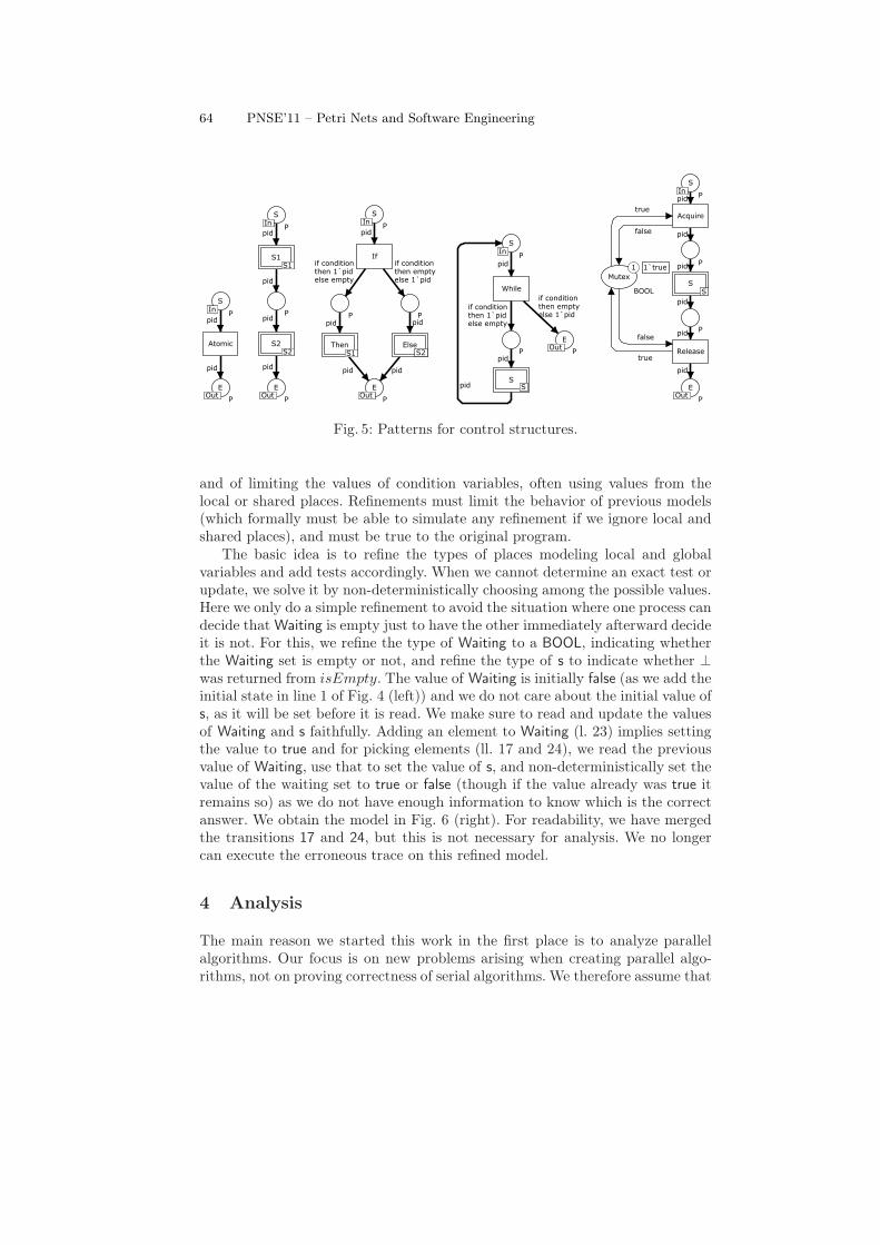
Extracting the control-flow consists of creating the process places and tran-sitions of the model. We do that using templates, very similar to the workflow-patterns [15] for low-level Petri nets. In Fig. 5 we show the patterns necessary totranslate programs using our simple pseudo-code language to a PP-CPN model.From left to right the patterns match an atomic action (Atomic), a sequence oftwo subprograms (S1;S2), a conditional branch (if condition then S1 else S2),a while loop (while condition do S), and a critical section (atomic S). Thetype P is the process colour set and for each pattern, the place S is the startplace and E the end place. All places created are process places except for theMutex place, which is a shared place. We put all processes on the start placeof the top level. We can add new templates or derive other constructs, such asa simplified conditional branch omitting the else path, a repeat/until loop, a forloop, and a for all loop.

In the initial abstraction, we translate a condition to an unbound booleanvariable in the PP-CPN model. We add a local place for each local variable anda shared place for each global variable. These are available on all subpages wherethey are within the scope. In the initial abstraction, we approximate the type


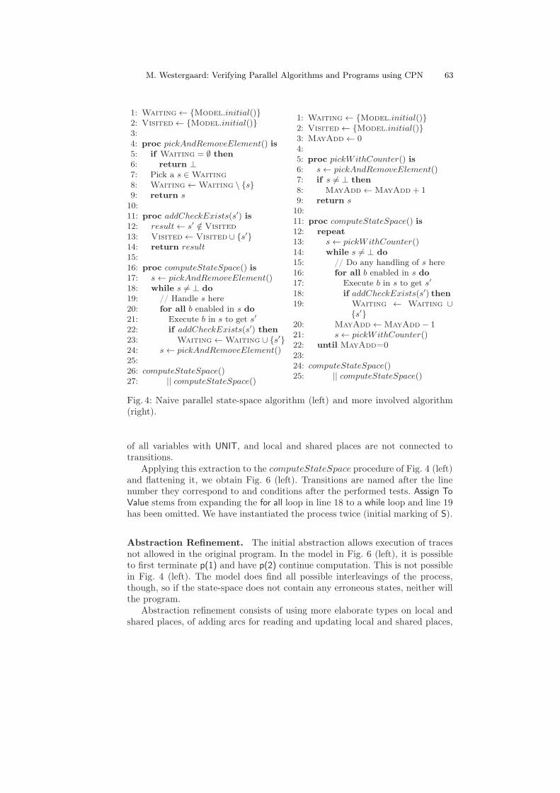
1: Waiting← {Model.initial()}2: Visited← {Model.initial()}3:4: proc pickAndRemoveElement() is5: if Waiting = ∅ then6: return ⊥7: Pick a s ∈Waiting8: Waiting←Waiting \ {s}9: return s

10:11: proc addCheckExists(s′) is12: result← s′ /∈ Visited13: Visited← Visited∪ {s′}14: return result15:16: proc computeStateSpace() is17: s← pickAndRemoveElement()18: while s 6= ⊥ do19: // Handle s here20: for all b enabled in s do21: Execute b in s to get s′

22: if addCheckExists(s′) then23: Waiting←Waiting ∪ {s′}24: s← pickAndRemoveElement()25:26: computeStateSpace()27: || computeStateSpace()

1: Waiting← {Model.initial()}2: Visited← {Model.initial()}3: MayAdd← 04:5: proc pickWithCounter() is6: s← pickAndRemoveElement()7: if s 6= ⊥ then8: MayAdd←MayAdd + 19: return s

10:11: proc computeStateSpace() is12: repeat13: s← pickWithCounter()14: while s 6= ⊥ do15: // Do any handling of s here16: for all b enabled in s do17: Execute b in s to get s′

18: if addCheckExists(s′) then19: Waiting ← Waiting ∪

{s′}20: MayAdd←MayAdd− 121: s← pickWithCounter()22: until MayAdd=023:24: computeStateSpace()25: || computeStateSpace()

Fig. 4: Naive parallel state-space algorithm (left) and more involved algorithm(right).

of all variables with UNIT, and local and shared places are not connected totransitions.

Applying this extraction to the computeStateSpace procedure of Fig. 4 (left)and flattening it, we obtain Fig. 6 (left). Transitions are named after the linenumber they correspond to and conditions after the performed tests. Assign ToValue stems from expanding the for all loop in line 18 to a while loop and line 19has been omitted. We have instantiated the process twice (initial marking of S).

Abstraction Refinement. The initial abstraction allows execution of tracesnot allowed in the original program. In the model in Fig. 6 (left), it is possibleto first terminate p(1) and have p(2) continue computation. This is not possiblein Fig. 4 (left). The model does find all possible interleavings of the process,though, so if the state-space does not contain any erroneous states, neither willthe program.

Abstraction refinement consists of using more elaborate types on local andshared places, of adding arcs for reading and updating local and shared places,


pid

pid

Atomic

EOut

P

SIn

PIn

Out

pid

pid

pid

pid

S2S2

S1S1

EOut

P

P

SIn

PIn

Out

S1

S2

pid

if conditionthen emptyelse 1`pid

pid

pid

pid

if conditionthen 1`pidelse empty

pid

ElseS2

ThenS1

If

P

EOut

P

P

SIn

PIn

Out

S1 S2

if conditionthen emptyelse 1`pid

pid

pid

if conditionthen 1`pidelse empty

pid

While

SS

EOut

PP

SIn

PIn

Out

S

pid

pid

pid

pid

pid

pid

P

P

P

SIn

PIn

BOOL

Acquire

false

true

trueMutex

false

true

SSS

Release

EOutOut

1 1`true

Fig. 5: Patterns for control structures.

and of limiting the values of condition variables, often using values from thelocal or shared places. Refinements must limit the behavior of previous models(which formally must be able to simulate any refinement if we ignore local andshared places), and must be true to the original program.

The basic idea is to refine the types of places modeling local and globalvariables and add tests accordingly. When we cannot determine an exact test orupdate, we solve it by non-deterministically choosing among the possible values.Here we only do a simple refinement to avoid the situation where one process candecide that Waiting is empty just to have the other immediately afterward decideit is not. For this, we refine the type of Waiting to a BOOL, indicating whetherthe Waiting set is empty or not, and refine the type of s to indicate whether ⊥was returned from isEmpty. The value of Waiting is initially false (as we add theinitial state in line 1 of Fig. 4 (left)) and we do not care about the initial value ofs, as it will be set before it is read. We make sure to read and update the valuesof Waiting and s faithfully. Adding an element to Waiting (l. 23) implies settingthe value to true and for picking elements (ll. 17 and 24), we read the previousvalue of Waiting, use that to set the value of s, and non-deterministically set thevalue of the waiting set to true or false (though if the value already was true itremains so) as we do not have enough information to know which is the correctanswer. We obtain the model in Fig. 6 (right). For readability, we have mergedthe transitions 17 and 24, but this is not necessary for analysis. We no longercan execute the erroneous trace on this refined model.

4 Analysis

The main reason we started this work in the first place is to analyze parallelalgorithms. Our focus is on new problems arising when creating parallel algo-rithms, not on proving correctness of serial algorithms. We therefore assume that


pid

pid

pid

pid

pid

pid

pid

pid

While 20

P

P

P

P

P P

P

S

P

P

23

If 22

if waitingNonEmptythen emptyelse 1`pid

if addCheckExiststhen emptyelse 1`pid

pid

pid

E

17

While 18

if waitingNonEmptythen 1`pidelse empty

pidif moreEnabledBindingsthen emptyelse 1`pid

if moreEnabledBindingsthen 1`pidelse empty

AssignTo Value

pid

21

pid

if addCheckExiststhen 1`pidelse empty

24

P.all()

s' PxU.all()

PxU

b PxU.all()

PxU

s PxU.all()

PxU

Visited ()

UNIT

Waiting ()

UNIT

21`p(1)++1`p(2)

21`(p(1),())++1`(p(2),())

21`(p(1),())++1`(p(2),())

21`(p(1),())++1`(p(2),())

1 1`()

1 1`()

if moreEnabledBindingsthen emptyelse 1`pid

(pid, isEmpty(waiting))

(pid, s)

waiting

(pid, s)

pid


pid

pid

pid

pid

pid

pid

pid


if isNotBottom(s)then emptyelse 1`pid

pid

if isNotBottom(s)then 1`pidelse empty

pid

pid

23

If 22

21

AssignTo Value

While 20

While 18

17/24

BOOL

Visited ()

UNIT

s all_b

PxB

b PxU.all()

PxU

s' PxU.all()

PxU

P

P

P

P

P

E

P

P

S P.all()

P


waiting

Waiting false

false

waiting orelse rand

1 1`()

21`(p(1),false)++1`(p(2),false)

21`(p(1),())++1`(p(2),())

21`(p(1),())++1`(p(2),())

21`p(1)++1`p(2)

1 1`false

Fig. 6: Control-flow of (left) and a simple refinement of the model (right).

algorithms are correct under certain mutual-exclusion assumptions, and searchfor such violations. We are also interested in potential dead- and live-locks. As-suming a valid refinement, we can ensure that absence of safety violations in themodel guarantees absence in the real program as we can simulate all executionsof the algorithm. This includes proving absence of mutual-exclusion violations.We cannot use our approach to ensure the absence of dead-locks, as we dealwith over-approximations of the possible interleavings and further restrictingthe behavior may introduce new dead-locks, but we can still find dead-locks andremove them from the implementation.

We can do state-space analysis of the derived models from Fig. 6, and obtaina state-space with 81 states for the abstract model (left) and a state-space with130 states for the refined model. As the models do not have any critical regions,they of course have no mutual exclusion violations.


Dead-locks and Live-locks. As all processes have a distinguished start andend-state, we can recognize dead-locks and live-locks in the model. A dead-lockis a state without successors (a dead state) where not all processes reside on E.Neither of the models in Fig. 6 has dead-locks; the model to the left has exactlyone dead state, where all process ids reside on E and the shared and local placesretain their initial marking. The model in Fig. 6 (right) also has one dead state,where all process ids reside on E, Waiting is true, s is true for all processes, andall remaining local and shared places have their initial value.

Live-locks are a harder to recognize. We only consider live-locks in the absenceof dead-locks. A model has a strong live-lock if the dead states of the model donot constitute a home space, i.e., if it is not always possible to reach one of thedead states. A strong live-lock in the model does not necessarily imply a live-lock in the original algorithm, but can be used to identify parts of the originalprogram that should be further investigated. None of the models in Fig. 6 havestrong live-locks.

A model may have a weak live-lock if its state-space has a loop. A loop mayalso just indicate that a loop may execute an unbounded number of times. Bothmodels in Fig. 6 have loops, but analysis shows that the transition While 20is impartial , i.e., that in any infinite execution it occurs an infinite number oftimes. This happens if we compute infinitely many successors (the state-spacehas infinitely many states), and makes sense in our algorithm.

A particular interesting kind of live-lock is a loop reachable from a statewhere E contains tokens. This means that even after one of the processes haveterminated, the amount of work done by another process is unbounded. We havealready seen that Fig. 6 (left) exhibits this due to too abstract modeling, i.e.,that process p(1) may decide that Waiting is empty initially and terminate, justto have p(2) decide it is non-empty and continue computation. We have seen thisis not possible in the original algorithm, which caused us to refine the model toFig. 6 (right). We would therefore expect that no such live-lock was presentin the refined model. Maybe surprisingly, one such does exist. This is seen byhaving p(1) check Waiting in 17/24, modify Waiting to be empty, and successfullycontinue. Then, p(2) checks Waiting, notices it is empty and terminates. Now,p(1) continues. This is also possible in Algorithm 4 (left), and even quite likelyas the two processes will test Waiting initially, one of them will consume the onlyelement it contains initially, and other processes terminate. This also occurred inreality in our first implementation of a parallel state-space exploration algorithmusing Algorithm 4 (left).

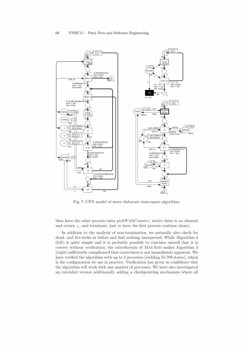
To fix this, we notice that the reason p(2) terminates prematurely in theprevious example is that it decided to terminate while p(1) can still add newstates to Waiting. The idea of an improved algorithm is to ensure that no pro-cesses may terminate when others may produce new states. This prompts us tomake Algorithm 4 (right). We reuse calculateStateSpace, addCheckExists, andpickAndRemoveElement from Algorithm 4 (left) and define a new procedurefor picking, pickWithCounter (ll. 5–9) which is used in place of the originalpickAndRemoveElement (ll. 13 and 21). We use MayAdd as a counter of the


number of processes which may add new states to Waiting. We add an addi-tional loop around the previous main loop ensuring we only quit when MayAddis zero. We inline the call to pickWithCounter for the translation and use amutex around the call to ensure atomicity.

We use the same approach to translate the model to a CPN model. Wemaintain the abstraction of Waiting and do no abstraction of MayAdd, i.e.,we increment and decrement it according to the algorithm. We implement themutex around the call to pickWithCounter as a place with type UNIT containinga single token acting as the mutex. We then obtain the model in Fig. 7. Wehave not completely flattened it for readability and to keep resemblance withthe previous models in Fig. 6. At the left we have the loop in lines 13–21,which mostly corresponds to Fig. 6 (right). The only changes are that aside fromrenaming transitions to correspond with the line numbers of Algorithm 4 (right),we have added a transition for the new line 20 causing some rerouting of the flow,added a place representing MayAdd, and changed 13/21 (named 17/24 in Fig. 6)to a substitution transition. We have modeled the new outer loop as a separatepage shown in Fig. 7 (top/right). We implement the semantics of a repeat/untilloop looping over the page in Fig. 7 (left). We share access to MayAdd. TheTest transition is explained later. The page corresponding to the substitutiontransition modeling pickWithCounter is shown in Fig. 7 (bottom/right). Again,we share access to a local place (s) and two shared places (MayAdd and Waiting).In all cases, the S and E places of a subpage is in port/socket relationship withthe input and output place of the corresponding substitution transition.

We can use state-space analysis to verify that (for this configuration) we donot violate the mutex property in pickWithCounter. The state-space for thismodel contains 399 states and 934 bindings. We can check this explicitly bylooking at the total number of tokens on the four unnamed places in Fig. 7(bottom/right). This is either 0 or 1, showing that never do we have more thanone process inside pickWithCounter. The Test transition in Fig. 7 is addedto easily test whether it is ever possible for a process to execute lines 15–20while another process has terminated, i.e., whether it is possible for a process toterminate while there is still work to do. The transition requires a token from E,i.e., a process that terminated and that the value of MayAdd is non-zero (this ishandled by the guard [n<>0], which has not been explained but exactly ensuresthis). If Test is enabled in any state, it means that a process has terminated whileanother has more work to do. State-space analysis shows this is not the case. Thisis also a safety property, so absence of violations in the model implies absence ofviolations in the original algorithm. We can prove the property without addingTest by searching for a state where E has tokens and Waiting is false or one ofthe unnamed places below While 14 contains tokens.

We can convince ourselves that the mutex around pickWithCounter is nec-essary by removing it and repeating analysis. We then get a state where Test isenabled, and we can verify the same error is present in the original model (haveone process enter pickWithCounter and consume the last element of Waiting,


pid


pid

n-1

true


waiting

pid

pid


pid

pid

pid

20

13/21pick

If 18

17

AssignTo Value

While 16

While 14

MayAdd

I/O

0

INT

EOut

P

Visited ()

UNIT

s all_b

PxB

b PxU.all()

PxU

s' PxU.all()

PxU

Waiting false

BOOL

SIn

P.all()

P

P

P

P

P

P

P

P

In

Out

I/O

pid

pid

n

19

pid

pid

if moreEnabledBindingsthen emptyelse 1`pid

pid

pid

(pid, s)



pick

1 1`0

1 1`()

21`(p(1),false)++1`(p(2),false)

21`(p(1),())++1`(p(2),())

21`(p(1),())++1`(p(2),())

1 1`false

21`p(1)++1`p(2)

pid

n

if n = 0then 1`pidelse empty

n

if n = 0then emptyelse 1`pid

pid

pid

pid

Test

[n<>0]

Until 22

13-2113-21

E

P

MayAdd

0

INT P

SP.all()

P

13-21

1 1`0

21`p(1)++1`p(2)

true

pid

pid


pid

n+1

n

(pid, s)

pid


pid

pid

pid

pid

pid

(pid, waiting)

waitingorelse rand

waiting

(pid, s)

ReleaseMutex

8

If 7

AcquireMutex

6

P

P

P

P

Mutextrue

BOOL

MayAdd

I/O

0

INT

EOut

P

SIn

P.all()

P

BOOL

s

I/O

all_b

PxBI/O

In

Out

I/O

Waiting

I/OI/O

true

false

false

false

1 1`true

1 1`0

21`p(1)++1`p(2)

21`(p(1),false)++1`(p(2),false)

1 1`false

Fig. 7: CPN model of more elaborate state-space algorithm.

then have the other process enter pickWithCounter, notice there is no elementand return ⊥, and terminate, just to have the first process continue alone).

In addition to the analysis of non-termination, we naturally also check fordead- and live-locks as before and find nothing unexpected. While Algorithm 4(left) is quite simple and it is probably possible to convince oneself that it iscorrect without verification, the introduction of MayAdd makes Algorithm 4(right) sufficiently complicated that correctness is not immediately apparent. Wehave verified the algorithm with up to 4 processes (yielding 55.709 states), whichis the configuration we use in practice. Verification has given us confidence thatthe algorithm will work with any number of processes. We have also investigatedan extended version additionally adding a checkpointing mechanism where all


threads are paused while Waiting and Visited are written to disk in a consistentconfiguration.

We also used the method to verify the implementation of a slightly simplifiedversion of the protocol for operational support developed in [16]. The protocolsupports a client which sends a request to an operational support service, whichmediates contact to a number of operational support providers. The protocoldeveloped in [16] has support for running all participants on separate machines,i.e., using asynchronous communication, but we are satisfied with an implemen-tation running the operational support server and providers on the same server.We therefore have to send fewer messages, but need to access shared data on theserver. We devised a fine-grained locking mechanism using the method devisedin this paper and proved that it enforced mutual exclusion and well as causedno dead-locks, increasing our confidence that the implementation works.

5 Conclusion and Future Work

We have sketched an approach for correct implementation of parallel algorithms.The approach allows users to extract a model from an algorithm written in animplementation or abstract language and verify correctness using state-spaceanalysis. The approach also facilitates the generation of skeleton implementationcode from the verified model using the approach from [13] as we rely on process-partitioned coloured Petri nets. Finally, we can also combine the two approaches,which facilitates writing an algorithm in an abstract language, extract a modelfor verification, and then extract a skeleton implementation.

Verification of software by means of models is not new. Code-generationfrom models have been used in numerous projects. The approach has beenmost successful for generating specification of hardware from low-level Petrinets and other formalisms to synthesize hardware such as computer chips [9,17].The approach has also been applied to high-level Petri nets to generate lowerlevel controllers [14] and more general software [13]. Model extraction was pi-oneered by FeaVer [6], which made it possible to extract PROMELA modelsfrom C code using user-provided abstractions, and Java PathFinder [7] whichdid the same for Java programs. The approach has successfully been refined us-ing counter-example guided abstraction refinement (CEGAR) [4] which was firstimplemented by Microsoft SLAM [1], which extracts and automatically refinesabstractions from C code for Microsoft Windows device drivers, and refined byBLAST [2]. While the tools for model-extraction support a full development cy-cle by abstraction refinement and reuse for modified implementations, the ideaof combining the two approaches is to the best of our knowledge new. The com-bination allows some interesting perspectives. The perspective we have focusedon in this paper is the ability to write an algorithm in pseudo-code, extract amodel from the code, and generate an implementation in a real language. An-other perspective is supporting a full cycle as well, where we extract a modelfrom a program, find and fix an error in the model, and emit code that is mergedwith the original code, supporting a cycle where we do not need to fix problems


on the original code but can do so at the model level. The use of coloured Petrinets instead of a low-level formalism allows us to use the real data-types used inthe program instead of abstractions, much like how FeaVer allows using C codeas part of PROMELA models, but with the added bonus that the operationsare a true part of the modeling language rather than an extension that requiressome trickery to handle correctly.

The work presented here is only in the initial stages, but looks very promising.We have several ideas for future work. Currently, we have to manually extractthe model from patterns. This is tedious and error-prone, and it would be niceto have automatic extraction. Such a translation should implement the patternsincluded in Fig. 5, but could also use explicit patterns for repeat/until loopsand other constructs. Given an implementation of the translation to and frommodels, we could look at supporting a full development cycle allowing us toupdate existing code with changes to the model.

An implementation could also implement reduction rules like the one weused to merge lines 17 and 24 in the model in Fig. 6 (right). We can also addsimplifications collapsing long traces of unconditional progress not modifyingany data to reduce the state-space without removing behavior. For example, inFig. 7 we can remove transitions Assign To Value and 17, merging the input placeof Assign To Value and the output place of 17, to obtain a smaller state-space of26.909 states for 4 processes, down from 55.709 states. We can also merge theacquisition of a lock with the first regular transition (merging the transitionsAcquire Lock with 6 in Fig. 7 (bottom/right)) and merging releases with thelast. This reduces the state-space to 14.841 states.

Currently, we provide abstractions manually. Like SLAM, we could easilyreplay found errors on the original code and provide assistance in the develop-ment of refinements, possibly even making them automatically. In our example,replaying the early termination error trace found in Fig. 6 (left) on Algorithm 4(left) would show that it is not possible for isEmpty to return false initially andthat it can only change from returning false to returning true if we execute line23. Even though we might not be able to provide the abstraction refinement inFig. 6 (right) fully automatically, providing such diagnostics can be very usefulfor the user for improving the refinement.

Our current method focuses on parallel algorithms with a fixed number ofidentical processes, but there is nothing in our approach preventing us fromextending this to also handle distributed settings with asynchronous communi-cation using buffer places and different kinds of processes; the code generationin [13] even supports that out of the box. While the fixed number of processesused in this paper works well for simple algorithms, more advanced algorithmsmay need to spawn processes. Nothing in our approach inherently forbids this,but the code generation in [13] does not support this out of the box. We believethat it should be quite easy to devise a construction for starting new processesand adapt the code generation to handle this.

One thing our approach does not support very well at the moment is intra-procedure calls. We can currently simulate this in simple cases by inlining pro-


cedure calls, but this is not possible when using recursion. One way to fix it isto view a recursive call as starting a new process for executing the child andwaiting for the result. If we support different kinds of processes, communicationbetween processes, and dynamic instantiation of processes, this should be easyto add.

References

1. T. Ball and S.K. Rajamani. The SLAM project: debugging system software viastatic analysis. In Proc. of POPL’02, pages 1–3. ACM Press, 2002.

2. D. Beyer, T.A. Henzinger, R. Jhala, and R. Majumdar. The Software ModelChecker BLAST: Applications to Software Engineering. STTT, 7(5):505–525, 2007.

3. J. Billington, M.C. Wilbur-Ham, and M.Y. Bearman. Automated protocol Verifi-cation. In Proc. of IFIP WG 6.1 5th International Workshop on Protocol Specifi-cation, Testing, and Verification, pages 59–70. Elsevier, 1985.

4. E. Clarke, O. Grumberg, S. Jha, Y. Lu, and H. Veith. Counterexample-GuidedAbstraction Refinement for Symbolic Model Checking. J. ACM, 50:752–794, 2003.

5. K.L. Espensen, M.K. Kjeldsen, and L.M. Kristensen. Modelling and Initial Vali-dation of the DYMO Routing Protocol for Mobile Ad-Hoc Networks. In Proc. ofATPN, volume 5062 of LNCS, pages 152–170. Springer, 2008.

6. The FeaVer Feature Verification System webpage. Online: cm.bell-labs.com/cm/cs/what/feaver/.

7. K. Havelund and T. Presburger. Model Checking Java Programs Using JavaPathFinder. STTT, 2(4):366–381, 2000.

8. G.J. Holzmann. The SPIN Model Checker. Addison-Wesley, 2003.9. IEEE Standard System C Language Reference Manual. IEEE-1666.

10. K. Jensen and L.M. Kristensen. Coloured Petri Nets – Modelling and Validationof Concurrent Systems. Springer, 2009.

11. L.M. Kristensen and K. Jensen. Specification and Validation of an Edge RouterDiscovery Protocol for Mobile Ad-hoc Networks. In Integration of Software Spec-ification Techniques for Application in Engineering, volume 3147 of LNCS, pages248–269. Springer, 2004.

12. L.M. Kristensen, J.B. Jørgensen, and K. Jensen. Application of Coloured PetriNets in System Development. In Proc. of 4th Advanced Course on Petri Nets,number 3098 in LNCS, pages 626–685. Springer, 2004.

13. L.M. Kristensen and M. Westergaard. Automatic Structure-Based Code Genera-tion from Coloured Petri Nets: A Proof of Concept. In Proc. of FMICS’10, LNCS,pages 215–230. Springer, 2010.

14. J.L. Rasmussen and M. Singh. Designing a Security System by Means of ColouredPetri Nets. In Proc. ATPN’96, volume 1091 of LNCS, pages 400–419. Springer,1996.

15. W.M.P. van der Aalst and K. van Hee. Workflow Management: Models, Methods,and Systems. MIT Press, 2002.

16. M. Westergaard and F.M. Maggi. Modelling and Verification of a Protocol for Op-erational Support using Coloured Petri Nets. In Proc. of ATPN, LNCS. Springer,2011.

17. A. Yakovlev, L. Gomes, and L. Lavagno. Hardware Design and Petri Nets. KluwerAcademic Publishers, 2000.


Towards Verifying Parallel Algorithms and Programs using …ceur-ws.org/Vol-723/paper5.pdf ·...

Documents

Transcript of Towards Verifying Parallel Algorithms and Programs using …ceur-ws.org/Vol-723/paper5.pdf ·...