Towards User Profile-based Interfaces for Exploration of Large Collections of Items

Claudia Becerra

Universidad Nacional de Colombia Bogotá - Colombia www.unal.edu.co

cjbecerrac@unal.edu.co

Sergio Jimenez Universidad Nacional de Colombia

Bogotá - Colombia www.unal.edu.co

sgjimenezv@unal.edu.co

Alexander Gelbukh Instituto Politécnico Nacional,

Centro de Investigación en Computación, Mexico, D.F

http://nlp.cic.ipn.mx/

gelbukh@cic.ipn.mx

ABSTRACT

Collaborative tagging systems allow users to describe and

organize items using labels in a free-shared vocabulary (tags),

improving their browsing experience in large collections of items.

At present, the most accurate collaborative filtering techniques

build user profiles in latent factor spaces that are not interpretable

by users. In this paper, we propose a general method to build

linear-interpretable user profiles that can be used for user

interaction in a recommender system, using the well-known

simple additive weighting model (SAW) for multi-attribute

decision making. In experiments, two kinds of user profiles where

tested: one from free contributed tags and other from keywords

automatically extracted from textual item descriptions. We

compare them for their ability to predict ratings and their potential

for user interaction. As a test bed, we used a subset of the

database of the University of Minnesota’s movie review system—

Movielens, the social tags proposed by Vig et al. (2012) in their

work “The Tag Genome”, and movie synopses extracted from the

Netflix’s API. We found that, in “warm” scenarios, the proposed

tag and keyword-based user profiles produce equal or better

recommendations that those based on latent-factors obtained using

matrix factorization. Particularly, the keyword-based approach

obtained 5.63% of improvement. In cold-start conditions—movies

without rating information, both approaches perform close to

average. Moreover, a user profile visualization is proposed arising

an accuracy vs. interpretability tradeoff between tag and keyword-

based profiles. While keyword-based profiles produce more

accurate recommendations, tag-based profiles seems to be more

readable, meaningful and convenient for creating profile-based

user interfaces.

Categories and Subject Descriptors H.3.3 [Information Storage and Retrieval| Information Search

and Retrieval]: Selection process; H.5.3 [Information Interfaces

and Presentation]: Group and Organization Interfaces–

Collaborative computing; H.5.2 [Information Interfaces and

Presentation]: User Interfaces

General Terms

Algorithms, Experimentation.

Keywords Recommender systems, collaborative filtering, collaborative

tagging systems, social tagging, user interfaces

1. INTRODUCTION An approach for improving the exploration of large collections of

items such as books (librarything.com), films (netflix.com),

pictures (flickr.com), research papers (citeulike.com) and web

bookmarks (del.icio.us) is the leveraging of collaborative

information from the users. This approach allows the knowledge

of certain individuals on certain items in the collection propagates

towards other users. In this way, a self-generated collaborative

intelligence guides users in their exploration by recommendations

tailored to their preferences and away from dislikes.

Currently, collaborative filtering approaches derive user profiles

and produce recommendations based primarily on user feedback

whether explicit (e.g. ratings, “likes”, tagging, reviews) or implicit

(e.g. web logs). As the time goes by, user profiles grow while

their preferences evolve. Generally, users are allowed to update

their explicitly given information with the aim of adjusting their

profiles to get better recommendations. In this scenario, when a

user wants to update his (her) profile, it depends—for instance—

on a large number of ratings making of this a difficult and even

overwhelming task. The users should make a significant number

of targeted edits in their profiles to obtain the desired effect. The

situation worsens in systems based on implicit feedback where

user profiles are not interpretable nor accessible by users.

Most of the state-of-the-art methods for collaborative filtering

build user profiles projected in latent factor spaces. These latent

factors reduce considerably the dimensionality of the user profiles

providing more accurate recommendations at the expense of

interpretability. Unfortunately, users cannot make modifications

on these low-dimensional and highly informative profiles. A first

step to tackle this issue could be the design of interfaces based on

interpretable user profiles. For instance Lops et al. [16] proposed a

system where the user profiles are defined in a space indexed by

keywords automatically extracted from textual item descriptions

—keyword-based user profiles. However, in many cases the

number of extracted keywords is similar or even larger than the

number of items in the collection making it difficult the

interaction of users with their profiles.

Alternatively, user profiles can also be built using tags [2]—tag-

based user profiles. These tags come from collaboratively tagging

systems [29], which allows users in large collections to label

items using a shared free vocabulary. As a result of this social

indexing process [10], the system gradually collects a social

index, which enables users to classify, visualize and query items

in a way that is both personalized and social. Unfortunately, social

indexes suffer of misspellings, typographical errors and extremely

particular tags, making of them a noisy resource for the

Decisions@Recsys’13. October 12--16, 2013, Hong Kong, China.

Paper presented at the 2013 Decisions@RecSys workshop in

conjunction with the 7th ACM conference on Recommender Systems.

Copyright 2013 for the individual papers by the papers' authors.

Copying permitted for private and academic purposes. This volume is

published and copyrighted by its editors.

9

construction of meaningful user profiles. Sen et al. (2009) [23]

proposed an entropy-based measure and a cleaning procedure for

detecting a community-valuable tag set from a noisy social index.

They obtained a clean set of 1,128 tags from nearly 30,000

different tags collected by the MovieLens1 system during the year

2009. Clearly, this tag set has a more convenient size for

designing user interfaces for customizing user profiles based on

social tags.

In this paper, we propose a method based on matrices for building

linear user profiles based either on social tags or on automatically

extracted keywords. From the users’ point of view, these profiles

behave as a linear simple aggregative weighting model SAW [28],

that is one of the most comprehensive method for multi-attribute

decision making [12]. So, the proposed method discovers the

prior weights, or the users’ affinity coefficients with tags or

keywords, that minimize the rating prediction error. These

produced profiles—SAW user profiles—can be used either to

invite users to interact with their own profiles or to explain the

recommendations given by the system.

To evaluate the performance of SAW user the profiles, they were

compared against user profiles based on latent factors obtained

using matrix factorization techniques [15], [4]. This comparison

was made in the rating prediction task for the movie domain. We

observed that the proposed methods outperformed or reached

similar results in cross-validation and cold-start evaluation

settings (respectively) in comparison with strong baselines. That

is the main contribution of this work: a collaborative method to

obtain simple aggregative weighting user profiles without

compromising rating prediction accuracy.

In addition, a visualization of user profiles is provided with the

aim of analyzing the potential of SAW user profiles for the

construction of user interfaces for recommender systems. In that

visualization the profile of a single user is shown as a list of tags,

or keywords, ranked by preference. We argue that the

hypothetical user interaction with the top and the bottom of that

list would provide a mechanism for updating his user profile with

little effort. Simultaneously, the profiles of the nearest users are

also shown as a collaborative resource for suggesting updates.

2. RELATED WORK There have been several works that let users directly interact with

keyword-based user profiles or tag-based user profiles. For

example, the work of Pazzani and Billsus (1997) [9] is the earliest

system that let users directly interact with their keyword-based

user profiles. In that work, users directly assess the conditional

probability of liking or disliking a resource given that a particular

word is found in the resource’s textual description. These user-

provided conditional probabilities are used as priors to train a

Naïve Bayes classifier that, using users’ ratings, estimates the

probability of liking or disliking the resource using keywords as

resource features. They found that these prior profiles increase the

accuracy of the recommendations obtained by the Naïve Bayes

classifier, mainly in cold-start scenarios [21] when users have not

yet given enough ratings.

1 http://www.movielens.org

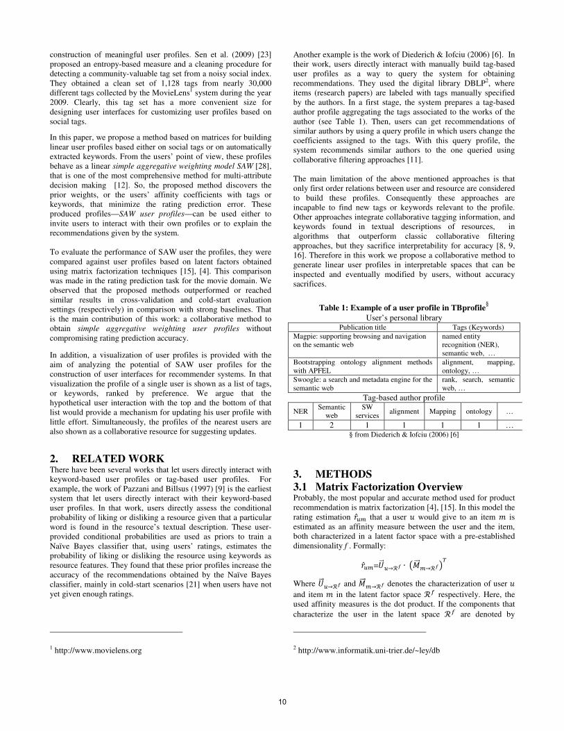
Another example is the work of Diederich & Iofciu (2006) [6]. In

their work, users directly interact with manually build tag-based

user profiles as a way to query the system for obtaining

recommendations. They used the digital library DBLP2, where

items (research papers) are labeled with tags manually specified

by the authors. In a first stage, the system prepares a tag-based

author profile aggregating the tags associated to the works of the

author (see Table 1). Then, users can get recommendations of

similar authors by using a query profile in which users change the

coefficients assigned to the tags. With this query profile, the

system recommends similar authors to the one queried using

collaborative filtering approaches [11].

The main limitation of the above mentioned approaches is that

only first order relations between user and resource are considered

to build these profiles. Consequently these approaches are

incapable to find new tags or keywords relevant to the profile.

Other approaches integrate collaborative tagging information, and

keywords found in textual descriptions of resources, in

algorithms that outperform classic collaborative filtering

approaches, but they sacrifice interpretability for accuracy [8, 9,

16]. Therefore in this work we propose a collaborative method to

generate linear user profiles in interpretable spaces that can be

inspected and eventually modified by users, without accuracy

sacrifices.

Table 1: Example of a user profile in TBprofile§

User’s personal library Publication title Tags (Keywords)

Magpie: supporting browsing and navigation

on the semantic web named entity

recognition (NER),

semantic web, …

Bootstrapping ontology alignment methods

with APFEL

alignment, mapping,

ontology, …

Swoogle: a search and metadata engine for the

semantic web

rank, search, semantic

web, …

Tag-based author profile

NER Semantic

web

SW

services alignment Mapping ontology …

1 2 1 1 1 1 … § from Diederich & Iofciu (2006) [6]

3. METHODS

3.1 Matrix Factorization Overview Probably, the most popular and accurate method used for product

recommendation is matrix factorization [4], [15]. In this model the

rating estimation �̂�� that a user � would give to an item � is

estimated as an affinity measure between the user and the item,

both characterized in a latent factor space with a pre-established

dimensionality f . Formally: �̂��=����→ℛ� ∙ �����→ℛ���

Where ����→ℛ� and ����→ℛ� denotes the characterization of user �

and item � in the latent factor space ℛ� respectively. Here, the

used affinity measures is the dot product. If the components that

characterize the user in the latent space ℛ� are denoted by

2 http://www.informatik.uni-trier.de/~ley/db

10

����→ℛ� = ����, ���, … , ����, and the item vector components are

denoted as ����→ℛ� = ����,���, … ,����, then the dot product

can be rewritten as: �̂��=∑ (��� ∙ ���)����

where the characterization of ���� and ���� vectors are found

minimizing the prediction error ��, which is calculated using the

following expression:

�� = !��� −#(��� ∙ ���)���� $

�

To avoid overfitting, it is common to introduce a regularization

coefficient % that penalizes the norm of the user and item vectors.

Thus, the regularized prediction error &�� is defined as: &�� = �� + % ()����→ℛ�)� + )����→ℛ�)�*

Finally, user and item vectors are found minimizing the

regularized prediction error over the set of known ratings.

min.��/,0��/ # !��� −#(��� ∙ ���)���� $

�1/2∈ℝ∧1/267 + % ()����→ℛ�)� + )����→ℛ�)�*

In this expression, we organize the known ratings in the matrix ℝ.×0 , of size � ×�, where � is the number of users and � is

the number of items. In this matrix, unknown ratings ��� are

assigned to 0, and known ratings are in the interval [1, 5].

3.2 Proposed Models 3.2.1 A Generic User Profiling Model In spite of the fact that it could be considered incorrect3, we will

use the canonical form of matrix factorization to express the

matrix of estimated ratings ℝ9.×0 as an affinity measure between

the user profile matrix :.� and the item profile matrix ;0�,

both characterized in the same latent factor space. Thus: ℝ9.×0 = :.×� ∙ �;0×���

Now, we can generalize this affinity measure to any space of

dimension < —denoted by ℛ=— using the expression:

3 It is important to keep in mind that, in order to calculate the

approximation of :.� and ;0� matrices, ratings ��� = 0 must

be ignored in the expression to minimize. This is why in the

recommendation study area, instead of using already implemented

matrix decomposition methods, it is preferable to use optimization

methods such us LBFGSB [5]. In these methods, the unknown

ratings are expressly filtered from the training matrix ℝ.×0.

Henceforth, the matrix notation will be used given the conceptual

simplicity that it provides for the further discussion. However, all

matrix factorizations will ignore unknown ratings ���.

ℝ9.×0 = :.×= ∙ (;0×=)�

Where :.×= is the ℛ=-based user profile matrix and ;0×= is the ℛ=-based item profile matrix. The matrix of user profiles in the

space ℛ=, :.×=, of size � × < can also be denoted as:

:.×= = ?��� ⋯ ��=⋮ ⋱ ⋮�.� ⋯ �.=C = D����→ℛE⋮���.→ℛEF

Where ��G represent the affinity coefficient between the user �

and the HIJ dimension in the space ℛ=, for values of � in K1, . . , �N and values of H in K1, . . , <N. In that notation, the vector ����→ℛE is the X-based user profile of user � in the space ℛ=.

Similarly, the ℛ=-based user profile matrix ;0×= can be denoted

as:

;0×= = ?��� ⋯ ��=⋮ ⋱ ⋮�0� ⋯ �0=C = D����→ℛE⋮���0→ℛEF

Where ��G denotes the relevance coefficient of the item � to the HIJ dimension in the space ℛ=, for values of � in K1, . . , �N and H

in K1, . . , <N. ����→ℛE represents the profile of the item m in the

space ℛ=.

Now, if we choose an interpretable space ℛ= in which the item

profile matrix ;0×= can be directly calculated, then all the user

profiles in :.×= can be obtained by the following expression: :.×= = ℝ.×0 ∙ ((;0×=)�)O�

Where ((;0×=)�)O� denotes the pseudo-inverse [18] of the

transposed item profile matrix characterized in ℛ=, and ℝ.×0 is

the matrix of known ratings.

3.2.2 SAW User Profiles

Once the user profiles are obtained the estimated ratings �̂�� can

be calculated with the expression: �̂�� = # ��G ∙ ��GG∈K�,…,|=|N

Therefore, from the point of view of decision making, it has the

well-known canonical form of the simple additive weighting

method (SAW) for multi-attribute decision making [13]. In this

model, a linear discriminative function is used to appraise each

resource assigning a value (weight) to each alternative.

Alternatives with higher values are preferred over alternatives

with lower values. Studies in the area [30], [1], [27] have shown

that the intuitiveness of the SAW method makes it more

preferable, for user direct interaction, than other less interpretable

non-linear methods.

Thus, our proposed model, behave as a SAW model for decision

making where: i) the appraisal of the resource is the rating of the

resource �̂��; ii) ratings are expressed as a weighted linear

combination of the resource features in the interpretable space ℛ=; and iii) weights or the affinity coefficients ��G are discovered

by the proposed model.

In the following subsections 3.2.3 and 3.2.4, we will explain how

this generic model can be applied in two different interpretable

spaces, namely keywords and tags. Besides, we will also show

how the proposed user profiles : can be used in combination with

the matrix factorization model to obtain rating predictions (see

11

subsection 3.2.5). To clarify the notation used in the following

sections, we will replace < for the specific size (dimensionality)

of the space in which we will focus the discussion. Thus, ℛQ will

be used instead of ℛ=, to denote he space of keywords.

Similarity, in subsection 3.2.4, the space defined by the tags will

be denoted by ℛ� .

3.2.3 Keyword-based User Profiles As mentioned before, the proposed model that automatizes the

process of construction of user profiles relies (in turn) in the

construction of the item profiles. Therefore, the matrix :.×Q

(keyword-based user profiles) is calculated using the matrices ;0×Q (keyword-based item profiles) and ℝ.×0 (known ratings)

using the following expression: :.×Q = ℝ.×0 ∙ ((;0×Q)�)O�

Most of the content-based approaches that build keyword-based

item profiles [16] use the vector space model [20] for representing

the textual descriptions of the items as vectors ����→ℛR.

Components of this vector, denoted by ��S, are values that

quantify the relevance of the word w to the item m. Thus, a value

close to 0 indicates that the word is not relevant to the item.

Negative values can also be used if polarized relevance scores are

available.

These relevance scores can be inferred from the occurrences of

the words in the collection of textual descriptions of the items.

The common practice to obtain relevance scores is to use the

popular tf-idf term weighting scheme [14] or weights derived

from the Okapi BM-25 retrieval formula [19]. These techniques

prevent that common words get high relevance scores and

promote less frequent words that occur systematically in particular

textual descriptions.

3.2.4 Tag-based User Profiles

Analogously to the keyword-based profiles, the :.� matrix with

the tag-based user profiles is calculated in the same way: :.×� = ℝ.×0 ∙ ((;0×�)�)O�

Where ;0×� is the matrix with tag-based item profile vectors ���0→ℛT, in which the individual ��I entries indicate the

relevance of the tag t to the item m.

The tag-based item profiles ����→ℛT can be obtained using several

techniques [16], [29]. The simplest approach consists in an item

profile based on Boolean occurrences. That is, set ��I = 1 when

the tag U has been applied to the item � and ��I = 0 otherwise.

It is important to note that the proposed method to obtain the tag-

based user profiles, using the pseudo-inverse, is equivalent to a

linear regression. Therefore, the tags should be independent

among them. That independence can be promoted grouping tags

that are morphologically related using stemmers and lemmatizers.

Lops et al. [17] went beyond grouping tags semantically related

using WordNet synsets [7].

Item profiles with graded, instead of Boolean relevance scores can

be obtained with more sophisticated methods. For instance, Vig et

al. (2012) [26] obtained the tag genome—a tag-based item profile

for movies—by training a support vector regressor [24]. The

training data came from a survey applied to users from the

MovieLens system. The users where asked to estimate the

relevance of the tags applied on selected movies. With these

answers and a set of features extracted from movie reviews,

textual descriptions, metadata and tag applications, among others,

they trained a regressor whose predictions were used as relevance

scores.

3.2.5 Hybrid and Updatable Rating Estimation The proposed method for generating the rating predictions is a

combination of matrix factorization (subsection 3.1) and the user

profiles proposed in subsections 3.2.3 and 3.2.4. The aim of the

method is three fold. First, we look for rating predictions as good

as the ones produced by matrix factorization. Second, the method

should be hybrid, that is, a combination of the collaborative

filtering approach of matrix factorization and the content

information from keywords or tags. Third, the users should be

able to edit their keyword-based (or tag-based) user profiles and

the rating predictions must be updated with little computational

cost. The method comprises four steps:

1. An initial matrix of rating estimations is obtained using

matrix factorization: ℝ9.×07 = :.×� ∙ �;0×���.

2. An initial matrix of keyword-based user profiles is obtained: :.×Q7 = ℝ9.×07 ∙ ((;0×Q)�)O�.

3. The matrix V.×Q, containing users edition operations to

their profiles (positive of negative differences) is added to

obtain updated user profiles: :.×Q = :.×Q7 + V.×Q.

4. Estimations are obtain by: ℝ9.×0 = :.×Q ∙ (;0×Q)�

These four steps can be expressed in a single expression: ℝ9.×0 = �ℝ9.×07 ∙ ((;0×Q)�)O� + V.×Q� ∙ (;0×Q)�

Note that ((;0×Q)�)O� ∙ (;0×Q)� ≅ X0×0 (the identity

matrix) only when the item profiles are linearly independent

among them. The contrary is the common case. Thus, this matrix

multiplication infers the affinities among the items induced by the

keywords content information. In a final post-processing step, the

values on each row in the output matrix ℝ9.×0 are standardized in

the interval [−1,1]. The final rating predictions are obtained

adding to each estimated rating the average rating of the movie

and the user’s bias. The user bias is the average deviation of the

user’s ratings against the average of the entire set of ratings. The

rating estimation using tag-based user profiles is the same but

replacing ;0×Q by ;0×�.

4. EXPERIMENTATION The experiments aim to evaluate the accuracy of the

recommendations produced by the proposed methods. This

section contains a comprehensive description of the data and the

evaluation measure used to compare the proposed models against

baselines.

4.1 Data

This subsection is intended to provide insight about how the used

dataset was obtained and preprocessed. Besides we provide

information about its content, size and distribution.

4.1.1 Movies Collaborative Data

The dataset of users, movies and ratings was obtained from a

production database dump of the MovieLens system in April

2012. From this dataset, we extracted a subset filtering by the

users and movies with more than 1,000 ratings. This filtering

produced a subset of 200 users, 1,462 movies and 150,915 ratings.

The rating scale in MovieLens is in the usual interval [1,5],

12

having 5 as the maximum grade of preference. The distribution of

ratings in our dataset is shown in Figure 1. The average number of

ratings per movie is 101.6 (σ = 37.5), and per user is 742.5 (σ = 188.5).

4.1.2 Textual Descriptions of the Movies

Textual descriptions were obtained from the synopsis field in the

movie records from the Netflix public API4 during the year 2012.

These texts were assigned to movies in the MovieLens dataset by

a mapping obtained through a research collaboration with the

GroupLens5 research group.

These textual descriptions were represented in a vectorial bag-of-

words model. The dimensionality of that representation was

reduced with the aim of obtaining a vocabulary based on

popularity and informativeness. Thus, a vocabulary of 5,848

words was obtained using the following series of preprocessing ad

hoc actions: (1) all characters were converted to lowercase

equivalents; (2) people first and last names were concatenated

with the underscore character; (3) numeric tokens were removed;

(4) 334 stop words taken from the source code of the gensim6

framework were removed; (5) words occurring in less than 10

synopses and in more than the 95% of the synopses, were

removed; and finally (6) all punctuation marks were cleaned.

The term weights used to register the relevance of a word in a

synopsis vector were obtained with the Okapi BM25 retrieval

formula [19] using the method proposed by Vanegas et al. [25].

Thus, the weight `(a, b) of a word a in a document (synopsis) b

is given by: `(a, b) = cde f� − bg(a)� h (i� + 1)Ug(a, b)j + Ug(a, b)

j = i� k(1 − l) + l bc(b)mnbc o

Where, bg(a) is the number of documents where a occurs, � = 1,462 is the number of movies, Ug(a, b) the number of

occurrences of word a in the document b, and mnbc = 33 is the

average document length. The additional used parameters were i� = 1.2 and l = 0.75 (see [e]). A pair of examples of the

resulting keyword vectors using the proposed method is shown in

Table 2. The aggregation of vectors obtained from synopses

produce the items profile matrix ;0×Q, whose dimensions are � = 1,462 movies (rows) by s = 5,848 words (columns). This

matrix is sparse, having only 0.518% of non-zero entries.

4.1.3 Social Tags

The tag set used to characterize the movies is the selection of tags

proposed by Vig et al. in “The Tag Genome” [26]. This tag set is a

subset of 1,128 tags out of nearly 30,000 unique tags freely

applied by 416 users in the MovieLens system. This subset was

obtained by removing tags with less than 10 applications,

misspellings, people names and near duplicates. Thereafter, they

selected the top 5% ranked tags with and entropy-based quality

measure proposed by Sen et al. [22]. Only 1,081 tags from the tag

genome’s set occurred in the 1,462 movies in the item-profile

matrix ;0�.

4 http://developer.netflix.com 5 http://www.grouplens.org 6 http://radimrehurek.com/gensim

There are 13,332 tag associations to the movies considered in this

study. 1,370 movies have at least one tag associated with an

average of 9.7 tags per movie (σ = 8.5). Besides, all tags were

assigned at least to one movie. The distribution of the tag

applications is considerably more uniform than the Zipf

distribution. Thus, the 108 more frequent tags (10%) represent

only the 42% of the tag associations. This can be roughly seen in

Table 3, which shows tag samples selected from uniformly

separated rank ranges. The association of movies and tags produce

the items profile matrix ;0� (1,462 movies by 1,082 tags) with

binary entries and a density of 0.844% (also very sparse).

Figure 1: Rating distribution in the used subset of MovieLens

Table 2: Examples of keywords in Netflix’s processed

movie descriptions

Movie: “Bewitched (2005)”

will_ferrell (0.237), jack (0.147), update (0.142), samantha

(0.131), sitcom (0.131), witch (0.119), nicole_kidman (0.119),

convinced (0.116), michael_caine (0.114), right (0.107), hoping

(0.105), know (0.103), career (0.099), perfect (0.098), doesnt

(0.097), actor (0.092), make (0.068), film (0.045)

Movie: “Rocky V (1990)”

burt_young (0.249), talia_shire (0.242), broke (0.15),

upandcoming (0.15), shots (0.15), boxer (0.15), crooked

(0.142), trainer (0.136), glory (0.136), accountant (0.131),

ended (0.131), lifetime (0.128), memory (0.124), training

(0.124), rocky (0.121), inspired (0.107), taking (0.101), career

(0.099), left (0.092), series (0.071), takes (0.063), finds (0.058)

Table 3: Samples of tags in the MovieLens tag set§

Rank Sample tags

1-3 based on a book (194), comedy (182), classic (143)

9-12 boring (107), 70mm (193), romance (98), quirky (91)

17-19 sci fi (78), stylized (64), adventure(62), humorous(62)

25-26 crime (53), sequel, tense, violence, remake (52)

34-35 animation (42), politics, satirical, war, hilarious (41)

42 bittersweet (34), gay, historical, musical, suspense

50 forceful (26), military, satire, small town, very good

59 cult classic (17), dark humor, earnest, epic, japan {17}

67 action packed(9), alien, aviation, based on comic {41}

75 3d(1), adoption, airplane, alcatraz, arms dealer: {80}

§ In parenthesis the number of movie associations to the tag; if missing,

then it is the same as the precedent. The number of tags in the same rank is

showed in curly brackets; if missing the listed tags are all the tags in that

rank.

4.2 Experimental Setup

12,98943,068 55,025

27,19310,229

����� ���� ��� �� �

13

To evaluate the performance of the proposed methods we

provided two scenarios of validation in 10 folds: cross validation

and product-cold-start [24]. In the cross validation scenario, the

ratings were divided in ten randomized folds. In each fold 90% of

ratings were used for training and the remaining 10% was used for

testing. In the product-cold-start scenario, the procedure for

extracting the training and test datasets is the same, but all the

ratings from the movies in the test set are removed.

The evaluation measure to assess the accuracy of the

recommendations is root-mean-square error (RMSE) defined as:

t�uv = w∑ (�̂�� − ���)�K1/2N∈IxyI|U zU|{

Where U zU is the test set of the ratings and |U zU| its cardinality.

Given that the methods proposed in section 3 provide rating

estimations standardized in [−1,1] interval, �̂�� is obtained

adding to these estimation the average of all the training ratings

and the user’s bias. Similarly, the baseline for the cold-start test

scenario is a simple recommender system that predicts ratings

based only on the average of all the training ratings plus the user’s

bias. The baseline method for the “warm”-start scenario is the

recommender system based on matrix factorization presented in

subsection 3.1. In all experiments, the number of latent factors

was set to 30, % = 0.07 and the objective function was minimized

using the LBFGSB optimization method [5].

Note that the matrix factorization method cannot be applied in the

cold-start scenario because movies without ratings cannot be

represented in the latent factors space. Consequently, for this

scenario, the method proposed in subsection 3.2.5 uses ℝ.×0

instead of ℝ9.×07 in the second step and the first step must be

skipped.

5. RESULTS AND DISCUSSION

5.1 Recommendations Accuracy

The results of our experiments are presented in Table 4. The first

two rows show the results for the proposed baseline methods for

each one of our test settings. The remaining two rows show the

results obtained by the proposed methods presented in subsection

3.2.4. For each system, the “RMSE” columns present the average

for the 10 folds and the columns labeled with "σ" reports the standard deviation.

Table 4: Rating Prediction Results

METHOD

COLD

START

WARM

START

RMSE σ RMSE σ

System average+user’s bias 1.065 0.022 - -

Matrix factorization - - 0.995 0.010

Keyword-based user prof. 1.052 0.015 0.939 0.016

Tag-based user profiles 1.062 0.021 0.985 0.012

Regarding the “warm” scenario (i.e. cross validation), the

obtained results show that the two proposed methods based on

user profiles outperformed the baseline matrix factorization

method. Particularly, the margin obtained by the keyword-based

user profile system was clearly significant, being more than 3

standard deviations apart. Clearly, the proposed methods reached

a performance level in the state of the art for the rating prediction

task. Unlike matrix factorization, our recommendations were

produced by a fully interpretable model suitable for better user

interaction and better explanations.

The cold-start evaluation setting was clearly more challenging.

Our systems barely overcame the proposed average-based

baseline. However, the proposed tag and keyword-based systems

have the potential to provide to the user mechanisms to get the

system “warmer” with little effort. Accurate methods such as

matrix factorization require a considerable number of initial

ratings before starting to produce good predictions. In contrast,

our methods provide a completely customizable user profile with

just a small number of initial ratings.

Comparing the tag-based and keyword-based models, the results

show that keyword-based user profiling performs better in

“warm” conditions and slightly better in “cold” conditions

5.2 Visualizing User Profiles

In order to visualize the profiles, we selected the User 156 from

the fold 1 in our dataset. We must say that users in our data are

completely anonymous. This user was manually chosen based on

the user-to-user pairwise Pearson correlation matrix obtained from

the keyword-based user profiles :.×Q. Comparing these

correlations we observed that the User 156 had high negative and

positive correlations against the other users. So, we considered

that the preferences and dislikes of this user was being shared by

several users and rejected by others. Consequently, we considered

him as an interesting candidate to be visualized. In Figure 2, the

keyword-based user profile of the User 156 is showed jointly with

his 10-nearest users according to the user-to-user correlation

matrix. The ranked list of keywords that this user prefers the most

is shown on the left side. The right side shows the list of his most

disliked keywords. The user profile is represented by the thick

black line. In its turn Figure 3, shows the same plots but using tag-

based user profiles instead of keywords.

Now it is possible to qualitatively compare a user keyword-based

versus a tag-based profile. From this comparison we observe that

User 156’s tag-based profile is more cohesive in comparison with

the word-based profile. This cohesiveness can be observed by the

semantic relatedness of the tag set. In this profile, 20 out of 40

tags preferred by User 156 are related to action and teens movies.

These tags are: Dark hero, Effects, Explosions, Indiana jones,

German, Drug addiction, Arms dealer, Weapons, Life & death,

Videogame, First contact, Comic book adapt, Bond, 007 series,

Stop motion, Fantasy world, Dreamworks, Video games, Harry

potter, Emma Watson. Regarding the keyword-based profile, the

keyword set doesn’t exhibit a clear pattern. Although we know

that these particular observations cannot be generalized, we think

that this observation opens an interesting research direction about

the necessity of measuring the semantic cohesiveness of the

produced profiles.

Concerning the potential of interaction we have not yet conducted

any experiments with users, but it seems reasonable that users will

understand the general interaction idea. It is expected that the

users will be prone to experiment modifying their own profiles

varying the level of preference or dislike for the more relevant

tags or keywords in their profiles. Also, it seems that the feature

of seeing the profile of similar users could motivate the desire to

interact with the interface. That is because, showing other people

behaviors and allows a kind of warm start with the system. New concerns arise from the observations of these profiles. For

instance, what should be done with “negative” tags that appear in

14

the list of preferred tags of users? This situation is illustrated by

the tag “boring!” in the User 156’s “likes” list.

Probably, this tag can be reasonable and predictive for some users,

so, maybe it shouldn’t be removed from the tag set. But trenchant

criticisms of user tastes should be prevented. A possible

alternative to this problem would be the use of a linear regression

algorithm, similar to the one used in a previous work [3], that

could estimate a weight for each tag for knowing if the tag is

intrinsically positive or negative. Thus, if a tag has a negative

connotation we could filter it from the list of “liked” tags.

Figure 2: Keyword-based profile for User 156

6. CONCLUSIONS We proposed a generic method to extract user profiles, in

interpretable spaces, in which it is possibly to directly characterize

items from the collection. The proposed user-profiling methods

were indexed in two different spaces: keywords and tags. Besides

the proposed models are suitable for user interaction in the user

profile component.

The proposed user-profiling methods were evaluated in a subset

of the MovieLens dataset and compared against strong baselines.

It was concluded that in “warm” scenarios both methods produce

recommendations with the same accuracy than those produced by

matrix factorization methods. In a cold-start scenario, both

methods performed slightly better than a recommender system

based on average ratings.

In the warm-start scenario, when the keyword-based profiling and

the tag-based profiling methods are compared, it was observed

that keyword-based method was considerably more accurate than

the matrix factorization method. The RMSE decremented by a

5.63% (more than 3 times σ), while the difference in the error

with the tab-based method was only 1.00%. Consequently, it is

possible to say that the proposed keyword-based method is able to

improve the matrix factorization approach.

Figure 3: Tag-based profile for User 156

Regarding the proposed visualization of the keyword-based and

the tag-based user profiles, we could observe that cohesion of the

profile is an important measure to have into account when two

profiles methods are compared. Non-cohesive profiles might be

misunderstood by users leading them to avoid the interaction with

those profiles. An interesting research question could be how to

discriminate cohesive profiles, from non-cohesive profiles.

The proposed approach also contributed to a better classification

of the content-based recommendation techniques, separating the

user-profiling task from the item-profiling task, suggesting a

uniform framework to share and compare the contributions made

on each one of the tasks.

7. ACKNOWLEDGMENTS

15

Our especial thanks to Prof. John Riedl and Daniel Kluver from

GroupLens, the University of Minnesota; Prof. Shilad Sen of the

Macalester College; and Prof. Fabio Gonzalez of the Universidad

Nacional de Colombia. The work was partially funded by the

Colombian Department for Science, Technology and Innovation

(Colciencias) via the grant 1101-521-28465 from “El Patrimonio

Autónomo Fondo Nacional de Financiamiento para la Ciencia, la

Tecnología y la Innovación, Francisco José de Caldas” and by the

Universidad Nacional de Colombia via the grant DIB QUIPU:

201010016956. The third author recognizes the support from

Mexican Government (SNI, COFAA-IPN, SIP 20131702,

CONACYT 50206-H) and CONACYT–DST India (grant 122030

“Answer Validation through Textual Entailment”).

7. REFERENCES [1] Adomavicius, G., Manouselis, N. and Kwon, Y. 2011.

Multi-Criteria Recommender Systems. Recommender

Systems Handbook. 769–803.

[2] Man Au Yeung, C., Gibbins, N. and Shadbolt, N. 2008. A

Study of User Profile Generation from Folksonomies.

SWKM (2008).

[3] Becerra, C., Gonzalez, F. and Gelbukh, A. 2011.

Visualizable and Explicable Recommendations Obtained

from Price Estimation Functions. Proceedings of the

Human Decision Making in Recommender Systems (2011),

27–34.

[4] Bell R.M., Koren Y. and C, V. 2007. The BellKor solution

to the Net Flix Prize. Technical report, AT&T Labs

Research. (2007).

[5] Byrd, R.H., Lu, P., Nocedal, J. and Zhu, C. 1995. A limited

memory algorithm for bound constrained optimization.

SIAM J. Sci. Comput. 16, 5 (Sep. 1995), 1190–1208.

[6] Diederich, J. and Iofciu, T. 2006. Finding Communities of

Practice from User Profiles Based On Folksonomies.

Proceedings of the 1st International Workshop on Building

Technology Enhanced Learning solutions for Communities

of Practice (2006).

[7] Fellbaum, C. ed. 1998. WordNet An Electronic Lexical

Database. The MIT Press.

[8] De Gemmis, M., Lops, P., Semeraro, G. and Basile, P.

2008. Integrating tags in a semantic content-based

recommender. Proceedings of the 2008 ACM conference

on Recommender systems (New York, NY, USA, 2008),

163–170.

[9] Guan, Z., Wang, C., Bu, J., Chen, C., Yang, K., Cai, D. and

He, X. 2010. Document recommendation in social tagging

services. Proceedings of the 19th international conference

on World wide web (New York, NY, USA, 2010), 391–

400.

[10] Hassan-Montero, Y. and Herrero-Solana, V. 2006.

Improving tag-clouds as visual information retrieval

interfaces. International Conference on Multidisciplinary

Information Sciences and Technologies (2006), 25–28.

[11] Herlocker, J.L., Konstan, J.A. and Riedl, J. 2000.

Explaining collaborative filtering recommendations.

(2000), 241–250.

[12] Hwang, C.L. and Yoon, K.M. 1981. Multiple Attribute

Decision Making. Methods and Applications. Springer-

Verlag, NY. (1981).

[13] Hwang, C.L. and Yoon, K.M. 1981. Multiple Attribute

Decision Making. Methods and Applications. Springer-

Verlag, NY. (1981).

[14] Jones, K.S. 1972. A statistical interpretation of term

specificity and its application in retrieval. Journal of

Documentation. 28, (1972), 11–21.

[15] Koren, Y., Bell, R. and Volinsky, C. 2009. Matrix

Factorization Techniques for Recommender Systems.

Computer. 42, 8 (Aug. 2009), 30–37.

[16] Lops, P., Gemmis, M. and Semeraro, G. 2011. Content-

based Recommender Systems: State of the Art and Trends.

Recommender Systems Handbook. F. Ricci, L. Rokach, B.

Shapira, and P.B. Kantor, eds. Springer US. 73–105.

[17] Lops, P., Gemmis, M., Semeraro, G., Musto, C., Narducci,

F. and Bux, M. 2009. A Semantic Content-Based

Recommender System Integrating Folksonomies for

Personalized Access. Web Personalization in Intelligent

Environments. G. Castellano, L. Jain, and A. Fanelli, eds.

Springer Berlin Heidelberg. 27–47.

[18] Penrose, R. and Todd, J.A. On best approximate solutions

of linear matrix equations. Mathematical Proceedings of

the Cambridge Philosophical Society. null, 01, 17–19.

[19] Robertson, S. 2005. How Okapi Came to TREC. TREC:

Experiment in Information Retrieval. MIT Press. 287–300.

[20] Salton, G., Wong, A.K.C. and Yang, C.-S. 1975. A vector

space model for automatic indexing. Commun. ACM.

18(11), (1975), 613–620.

[21] Schein, A., Pennock, D. and Ungar 2002. Methods and

metrics for cold-start recommendations. SIGIR (2002).

[22] Sen, S., Harper, F.M., LaPitz, A. and Riedl, J. 2007. The

quest for quality tags. Proceedings of the 2007

International ACM Conference on Supporting Group Work

(2007), 361–370.

[23] Sen, S., Vig, J. and Riedl, J. 2009. Learning to recognize

valuable tags. Proceedings of the 13th International

Conference on Intelligent User Interfaces (Sanibel Island,

Florida, USA, 2009), 87–96.

[24] Smola, A.J. and Schölkopf, B. 1998. A Tutorial on Support

Vector Regression,. Royal Holloway College, London,

U.K., NeuroCOLT Tech. Rep..TR 1998-030, 1998. (1998).

[25] Vanegas, J.A., Caicedo, J.C., Camargo, J.E. and Ramos-

Pollán, R. 2012. Bioingenium at ImageCLEF 2012:

Textual and Visual Indexing for Medical Images. CLEF

(Online Working Notes/Labs/Workshop) (Rome, Italy,

2012).

[26] Vig, Jesse, Sen, S. and Riedl, J. The Tag Genome:

Encoding Community Knowledge to Support Novel

Interaction. ACM Transactions on Interactive Inteligent

Systems. 2, 3.

[27] Yeh, C.H. 2002. A problem based selection of multi-

attribute decision-making methods. International

Transactions in Operational Research. 9, 2 (Mar. 2002),

169–181.

[28] Yoon, K. and Hwang, C. 1995. Multiple Attribute Decision

Making. An introduction. Sage university papers series,

no. 07-104. Thousand Oaks, CA: Sage Publications.

(1995).

[29] Zhang, Z.-K., Zhou, T. and Zhang, Y.-C. 2011. Tag-Aware

Recommender Systems: A State-of-the-Art Survey.

Journal of Computer Science and Technology. 26, 5 (Sep.

2011), 767–777.

[30] Zopounidis, C. and Doumpos, M. 2002. Multicriteria

classification and sorting methods: A literature review.

European Journal of Operational Research. 138, 2 (Apr.

2002), 229–246.

16