Towards the Precision Spectroscopy of a Single Molecular Ion
219
NORTHWESTERN UNIVERSITY Towards the Precision Spectroscopy of a Single Molecular Ion A DISSERTATION SUBMITTED TO THE GRADUATE SCHOOL IN PARTIAL FULFILLMENT OF THE REQUIREMENTS for the degree DOCTOR OF PHILOSOPHY Field of Physics By Yen-Wei Lin EVANSTON, ILLINOIS December 2016
Transcript of Towards the Precision Spectroscopy of a Single Molecular Ion

NORTHWESTERN UNIVERSITY
Towards the Precision Spectroscopy of a Single Molecular Ion
A DISSERTATION
SUBMITTED TO THE GRADUATE SCHOOL
IN PARTIAL FULFILLMENT OF THE REQUIREMENTS
for the degree
DOCTOR OF PHILOSOPHY
Field of Physics
By
Yen-Wei Lin
EVANSTON, ILLINOIS
December 2016

2
c Copyright by Yen-Wei Lin 2016
All Rights Reserved

3
ABSTRACT
Towards the Precision Spectroscopy of a Single Molecular Ion
Yen-Wei Lin
This dissertation presents some development of the single molecular ion precision spec-
troscopy experiment including construction of the project, spectroscopy state readout,
and production of ultracold molecules. Such molecular ion spectroscopy aims at testing
fundamental physics such as probing the time variation of electron-proton mass ratio.
The theories and characterization of ion traps are first discussed along with informa-
tion regarding building the ion trapping systems. Then, routines in this project such as
loading ions, Doppler laser cooling, excessive micromotion compensation, secular motion
detection, and fluorescence imaging are deliberated.
In the state readout experiment, the coherent motion of a single trapped barium ion
(Ba+) resonantly driving by a radiation pressure is studied. By scattering of order only
one hundred photons, the radiation pressure is able to seed a laser-cooled ion with a
secular oscillation that is detectable by the Doppler velocimetry technique after proper

4
motional amplification. This seeding method provides a mapping between the ion’s in-
ternal configuration and its secular motion and can be used to read out the spectroscopy
results from a single non-fluorescing ion with a partially-closed cycling transition.
The work of ultracold molecule production is done with silicon monoxide ions (SiO+),
which has a strong vibration-conserved spontaneous decay branching. Therefore, by op-
tically pumping the rotational cooling transitions in SiO+ with a broadband radiation,
the population can be eciently driven into the ground rotational state before falling
into other manifolds. To avoid the rotational heating transition, the broadband source,
derived from a femtosecond pulsed laser, is spectrally filtered using an ultrashort pulse
shaper.

5
Acknowledgements
This dissertation is a compilation of a few years of my experimental works in the
laboratory and I would not be able to make most of it without many people’s help.
I would like to first express my great gratitude to my advisor Prof. Brian Odom for
the continuous support in all dimensions. He recruited me into his group to start building
the project from scratch and coached me during the course. Prof. Odom’s knowledge and
techniques, research experience, and scientific perspective certainly had a strong impact
on my professional development.
Helps from members of the Odom group were significant as well. People in the group
have all kinds of expertise and there are a lot I can learn from them no matter how long
I have been in the business.
Support from outside the group was equally important. The experience I received
from Prof. Ite Yu and Prof. Jow-Tsong Shy’s training and mentoring at National Tsing
Hua University, Hsinchu, Taiwan quite contributed to my dissertation work in the early
stage. Also, a special thank goes to Ms. Vicki Eckstein from the department’s business
oce, who helped us deal with endless purchasing issues.
I was, fortunately, to be accompanied by my wife, Yu-Han Jao, when completing my
doctoral dissertation. She has been sharing a lot of the stress coming from my work and
helping me stay positive.
Finally, thanks to my wonderful parents for everything they have done for me.

6
Table of Contents
ABSTRACT 3
Acknowledgements 5
List of Tables 9
List of Figures 11
Chapter 1. Introduction 19
Chapter 2. Ion Trapping 24
2.1. Ion Trap Basics 24
2.2. Trap Potential Simulation 29
Chapter 3. Apparatus for the Single Ion Trap 41
3.1. The Single Ion Trap 41
3.2. Trap Electrical 48
3.3. Barium Oven 55
3.4. Laser Systems 56
3.5. Laser Stabilization 58
3.6. Fluorescence Detection 60
Chapter 4. Single Ion Experiments 63

7
4.1. Loading an Ion 64
4.2. Laser Interaction with the Barium Ion 65
4.3. Laser Cooling 72
4.4. Photon Counting - Time Correlation 74
4.5. Micromotion compensation 77
4.6. Secular Oscillation 80
Chapter 5. Coherent Motion Single Ion State Readout 84
5.1. Motivation 84
5.2. Pulse-Driven Oscillator 85
5.3. Experimental Setup 91
5.4. Coherent Motion Amplification 93
5.5. Experiment Results 94
5.6. Spectroscopy Application 96
5.7. Error Sources and Improvement 98
5.8. Outloook 100
Chapter 6. Apparatus for the Molecular Ion Trap 102
6.1. The Molecular Ion Trap 102
6.2. Lasers 106
6.3. Fluorescence Detection 107
Chapter 7. The Molecular Ion Trap 112
7.1. Trapping Barium Ions 112
7.2. Loading SiO+ 114

8
7.3. Mass Spectrometry: Q-Scan 117
Chapter 8. SiO+ Experiments 122
8.1. Level Structure 123
8.2. Transitions in SiO+ 126
8.3. Internal State Cooling 131
8.4. Relaxation and Decoherence 141
8.5. On the Horizon 147
Chapter 9. Spectral Filtering 152
9.1. Introduction 152
9.2. The Spectral Filtering Setup 155
9.3. Setup 157
9.4. Evaluation and Calibration 163
9.5. Improvement 170
References 172
Appendix A. Fluorescence from a Three-level System 180
Appendix B. Finite Element Analysis of the Trap Potential 186
Appendix C. Drawings 203

9
List of Tables
2.1 The visualizations and the representations of m
l
for l 8. 36
2.2 The coecients of the multipole expansion in Eq. (2.18) with a cuto↵
at l = 8. In B1, RF electrodes in the (+x,+y) and (-x,-y) quadrants
are held at 1 while all other boundaries are at zero. In B2, RF
electrodes in the (-x,+y) and (+x,-y) quandatnts are charged. In B3,
the endcap electrodes are charged. In this simulation and analysis,
the length unit is mm. Only those points withinp
x2 + y2 < 0.2mm
and |z| < 0.8mm are included in the fitting. 39
3.1 Skin depth and AC resistance 44
4.1 Frequency response 83
5.1 Modeled contribution of various noise sources to the distribution
width of the modulation amplitude, for n
= 150 yielding h = 0.20.
Data is integrated over N excitation/detection cycles, with initial ion
temperature 360 µK, ts
= 40 µs, ta
= 10ms, and ga
= 2.5. For N = 1,
consider only the noise intrinsic to ideal single-shot excitation, say,
for perfect fluorescence collection or for sustained oscillation during
detection. For N = 40, there are 1000 fluorescence photon counts

10
spread over 20 timing bins. The last line represents the quadrature
addition of all sources. 99
8.1 Spectroscopic constants of the X, A, and B state in the SiO+ 125
8.2 Decay rates of some relavent decay channels in SiO+ . These rates
were calculated in-house. 128
B.1 Fitting region (x, y, z) | px2 + y2 < 1.5, |z| < 5 197
B.2 Fitting region (x, y, z) | px2 + y2 < 1.6, |z| < 9 202

11
List of Figures
2.1 Trap RF electrodes configuration 25
2.2 Stability diagram 28
2.3 A sample basis function in the two dimensions. 32
2.4 The trap geometry set up for the FEM simulation. Top: input
geometry. Bottom: the mesh. 34
3.1 Single ion trap outline 43
3.2 Tungsten wire electropolishing 45
3.3 Trap assembly 47
3.4 Outline of a helical resonator. (From Macalpine and Schildknecht
(1959, Fig. 2)) 49
3.5 Helical resonator design chart. (From (Macalpine and Schildknecht,
1959, Fig. 4)) 50
3.6 The helical resonator used to drive the single ion trap. 51
3.7 RF resonant circuit with a helical resonator 52
3.8 RF voltage calibration 53
3.9 High voltage regulator 54

12
3.10 The DC low-pass filtering circuit. V: DC voltage supply. C: 22 µF
capacitor. R: 50 k resistor. EC: endcap electrode. RF-trap: nearby
RF electrodes. The box indicates the filter box. 55
3.11 (a) Alumina tubing with tungsten coil as the barium oven. (b) The
apertures for the oven output. 56
3.12 Drift of the wavelength meter locking mechanism. 59
3.13 Imaging optics for the single ion experiment. 61
4.1 A trapped single Ba+ was first observed in the single ion trap at
around 2pm on September 2, 2011. 63
4.2 Stability region for Vrf and Vec. 64
4.3 Partial level diagram of Ba+. 66
4.4 CPT resonance observed by the laser-induced spectroscopy of Ba+. 71
4.5 Detect micromotion by autocorrelation. 79
4.6 Micromotion amplitude as a function of bias DC 80
4.7 Tickling on end cap 81
4.8 Autocorrelation function of the oscillating ion. 82
5.1 Modeled response of the Ba+ oscillator to a pulsed drive with 10%
duty cycle (gray band), with realistic drive parameter = 2.67 nm,
and initial conditions 0 = 122 and A0 = 34 nm (V0 = 0.2m/s),
typical of Doppler cooling. Results from the simulation (points)
13
deviate from the model of Eq. (5.20) (lines) because of noise in photon
scattering. 91
5.2 Experimental timing sequence. 92
5.3 Fluorescence modulation. (a) The ion is bright to the seeding laser.
(b) The ion is dark to the seeding laser. 94
5.4 Measured modulation amplitude mean (points) and standard
deviation (bars) versus seeding duty cycle, with seeding time varied to
maintain D ts
= 4 µs; data were collected over 30 trials. Averaging
Eq. (5.20) over initial phases and fitting for amplification-stage gain
yields the solid curve. 95
5.5 Modulation amplitude versus seeding time, when the seeding pulses
excite an S-state ion (red), and when the ion is shelved in the D-state
(blue). Each point is the average of 30 measurements, with the
vertical bars showing the distribution standard deviation (rather than
the error on the mean). The predicted response (black curve) is from
Eq. (5.20), fitting for amplification-stage gain. 96
5.6 Distribution of the modulation amplitudes, measured after seeding
the motion for 40 µs (red histogram) and for an unseeded ion (blue
histogram). The simulation (solid curves) accounts for noise in ion
dynamics and shot noise in detection. Amplification gain is the single
fit parameter. 97

14
5.7 Determination of modulation index from data with 30 average counts
per bin. 98
6.1 Molecular ion trap outline 103
6.2 RF source with toroidal inductor. 104
6.3 Imaging system for the molecular ion trap. (1) Single ion source, N.A.
= 0.22. (2) Vacuum viewport; fused silica, about 10mm thick. (3)
f=100mm achromatic doublet. (4) f=200mm achromatic doublet. (5)
f=50mm achromatic doublet. (6) Dichroic mirror transmits 493 nm
and reflects 385 nm. (7)(8) f=125mm achromatic doublet. 108
6.4 TRA of imaging system 110
6.5 Some images of ions with optical aberration 111
6.6 Eciency vs ROI size 111
7.1 laser cooled barium ions 114
7.2 The mass spectrometry of the ablation product on RGA. 115
7.3 Potential energy curves in the neutral SiO. From Oddershede and
Elander (1976). 117
7.4 SiO REMPI spectrum. 118
7.5 SiO+ dark core. 118
7.6 Stability region and the q-scan. 119
7.7 trap and cem 121
7.8 The q-scan data 121

15
8.1 Potential energy curves of SiO+. 125
8.2 reference spectroscopy signal 131
8.3 SiO+ laser-induced fluorescence spectrum in XB, (00). 132
8.4 Population distribution in the rotational states of SiO+ at 300K
(green) and 1000K (magenta). The P-branch (purple) and R-branch
(blue) rotational transitions in the BX, (00) band are shown as well.133
8.5 Rotational cooling illustrated. 134
8.6 Vibrational repumping 137
8.7 Data of cooling AlH+. Figure reproduced from Lien et al. (2014).
Dark red: AlH+’s rotational levels are thermally populated up to
N = 7 at the room temperature. Green: Cooling on the P-branch
but the P(1) transition results in population in the N=0 and N=1.
Blue: Further driving the P(1) transition causes the parity flipping
via the relaxation through X, v=1 and put the population completely
in N=0. 140
8.8 Relaxation time due to the spontaneous decay and the BBR-induced
transition. 144
8.9 Zeeman e↵ect 147
8.10 SiO+ dissociation cross-sections from B2 to (2)2 and (3)2. 150
9.1 Rotational cooling with spectral-filtered broadband source. In this
example, relevant transitions from A21/2, v0=0 X21/2, v
00=0
band in the AlH+ are shown as vertical bars at the bottom. P-branch

16
is the rotational cooling transitions, while Q- and R-branch are the
opposite. An unfiltered UV femtosecond laser (spectrum shown as
dashed line) drives all transitions thus provides no cooling e↵ect.
A filtered source (spectrum shown as solid line) drives only cooling
transitions and hence slows down the molecule’s rotation. 153
9.2 Schematic of our spectral filtering setup. fs-laser: mode-locked
femtosecond laser; WP: half-wave plate; XTAL: BBO SHG crystal;
L1-4: lens; M1-3: mirrors (M3 is concave). G1 and G2 are reflective
di↵raction gratings; C: fiber coupler. See text for detailed discussion. 156
9.3 Microscope images of three samples of razor blades used in this
experiment. While we image the blades (gray area) in front of a dark
background, the boundary between two areas is due to the blade
edge. It is easy to see the fuzziness of the blade edge is around 1 µm,
smaller than the focal spot size ( 10 µm) in our setup. 160
9.4 Some possible scenarios regarding dispersion in the 4-f line. The red
and the blue lines represent the propagation path of two di↵erent
spectral components. (a) is an ideal case where the input beam is
dispersion-free and G1=G2 and L2=L3. In (b), the alignment of some
components is o↵, and hence the output beam derives dispersion.
In general, as in (c), the source of dispersion can come from the
input beam and errors from components and alignment. However,
dispersion can be compensated by properly aligning the location and
the di↵raction angle of the grating G2. 162

17
9.5 Schematic of our spectrometer. C: fiber output coupler; L5-6:
collimation lens; G3: di↵raction grating; L7: focusing lens; CCD:
linear camera. 164
9.6 Intensity profile on the focusing plane of a narrowband laser, recorded
by a line camera. A large input beam size wi
= 12.1 mm is used in
the right panel, and causes the focal spot to be less compact. While
in the left, a permissible beam size wi
= 6.8 mm is used, and the focal
spot profile is fairly close to Gaussian. 165
9.7 (a) Consistency of spectrometer resolution over its measurement
range. In this test, we simulate di↵erent narrowband laser wavelengths
by rotating the grating, as if the di↵raction angle is changed due to
another wavelength. (b) Spot profiles for data #1 (left-most), #5
(middle), and #9 (right-most) from the data sequence in (a). The
horizontal axis is the pixel number on the linear camera. The spots
in the upper row are focused by the doublet lens and those in the
bottom row are focused by the singlet lens. The width of each plot is
30 pixels. 167
9.8 Spectrum of the original and filtered light. 169
9.9 Cuto↵ resolution versus mask longitudinal position. 169
9.10 cuto↵ resolution versus di↵erent cuto↵ frequency. 170

18
A.1 (Upper plot) Fc
versus laser intensity c
/c
. (Lower plot) Excitation
state population versus laser intensity c
/c
. b
= 0 and c
= 0 in
both plots. 183
C.1 Macro stand for RF electrodes - sheet 1 204
C.2 Macro stand - sheet 2 205
C.3 Macro stand for endcap electrodes 206
C.4 Trap base plate 207
C.5 Single ion trap assembly - sheet 1 208
C.6 Single ion trap assembly - sheet 2 209
C.7 Single ion trap assembly - sheet 3 210
C.8 Single ion trap assembly - sheet 4 211
C.9 Trap stand 212
C.10 6CF flange 213
C.11 Doubler - sheet 1 214
C.12 Doubler - sheet 2 215
C.13 Doubler - sheet 3 216
C.14 Doubler - sheet 4 217
C.15 Cover for the doubler 218
C.16 Crystal holder 219

19
CHAPTER 1
Introduction
Ultracold molecule is the new frontier in many fields. In the researches of quantum
information processing, the interaction between quantum bits can be realized by the large
dipole moment from the molecules. With the ability of quantum control of atoms and
molecules, chemistry can be studied with specific initial states in contrast to the thermal
population distribution. Molecules also provide additional advantages for spectroscopy
experiments of searching the permanent dipole moment and other testings of the funda-
mental physics, which is one of the focus in this research group.
Proton-to-Electron Mass Ratio
The proton-to-electron mass ratiomp
/me
µ is one of the fundamental constants that
describes the structure of matters. Its current value is 1836.152 673 771(7) (Sturm et al.,
2014). Theories of time-varying proton-to-electron mass ratio involve physics beyond the
Standard Model, which were reviewed in, e.g., Uzan (2011); Ubachs et al. (2016). Here,
I only briefly summarize from the experimental aspect.
The drift of µ can be probed by measuring the change of transition frequency in an
atomic or a molecular system. However, only the drift of a dimensionless quantity can be
reliably used to infer a time variation. Hence, to find the drift of µ, one must compare
the change among di↵erent transitions.

20
In the atomic system, the dependence on µ shows up in the transition between two
hyperfine states along with the fine structure constant ↵. However, hyperfine transitions
also have state-dependent components such that the ratio between two hyperfine tran-
sitions is not solely a function of µ. The determination of these other factors heavily
relies on the theories. Therefore, the time variation of µ measured in an atomic system is
oftentimes strongly model-dependent. The measurement is, however, model-independent
in a molecular transition as the ratio between rotational or vibrational transitions has a
pure dependence on the mass ratio: µ1/2 for the vibrational transitions and µ1 for the
rotational transitions (Flambaum and Tedesco, 2006). Thus, probing a drifting µ in a
molecular system is an advantage.
The major approach for measuring µ0/µ is by the astronomical observations. In some
measurements where the emission of H2 from the early Universe is compared to the lab-
oratory spectroscopy results. |µ/µ| is bounded by 5 106 over the 1010-year timespan,
or |µ0/µ| < 1016 per year, according to those measurements (see Ubachs et al. (2016)
for an overview). Yet, probing such tiny variation within a much shorter timeframe by a
tabletop experiment has recently become feasible due to the development of high preci-
sion atomic clock. For example, a Yb+ clock experiment has constrained the fractional
variation to be less than 1016/yr as well (Godun et al., 2014). In a di↵erent experiment,
Shelkovnikov et al. (2008) performed precision spectroscopy with SF6 molecular beam and
obtained 1014/yr fractional drift, which is one of the first measurements in a molecular
system. The measurement sensitivity will be advanced once we applied the precision ion
clock technique to a molecular ion.

21
Precision Spectroscopy
Single ion precision spectroscopy is the primary goal of our laboratory. We choose
to work with ionic species for the extreme long holding time in an ion trap. Besides,
minimization of the systematic errors is much easier for a localized single ion, which
makes the coherence time much longer than that of a cloud.
One of the challenges in the single ion spectroscopy is collecting the signal. Precision
laser spectroscopy usually involves detecting the fluorescence, which is an ecient and
least destructive state readout approach. However, most of the molecular species do
not have a closed transitions to generate a strong fluorescence signal. This obstacle
can be overcome by co-trapping the spectroscopy species with an additional ion, often
called the logic ion, that has good cycling transitions. Through their mutual Coulomb
interaction, the two ions share the common motional modes. First of all, the motion of
the spectroscopic ion can be therefore cooled by laser cooling the logic ion, known as the
sympathetic cooling. Furthermore, by driving transitions that couples the internal state
of the spectroscopic ion and the motional mode, the information of the internal degree of
freedom is mapped to the logic ion, which can be probed easily.
High precision single ion spectroscopy utilizing this scheme has been demonstrated in
Schmidt et al. (2005); Rosenband et al. (2008); Chou et al. (2010), for instance. In these
experiments, the spectroscopy of a single Al+ displayed a 1018 fractional uncertainty.
If the technology can be applied to the molecular ion spectroscopy to reach a similar or
better performance, this tabletop spectroscopy experiment will be able to perform some
of the stringent tests of the fundamental physics.

22
Cooling of Molecules
Another key towards the precision spectroscopy is to prepare the sample into a single
quantum state. Getting an atomic species into a single state by optical pumping is usually
easy due to the simple structure. However, optical pumping of a molecule is quite trickier
due to the additional vibrational and rotational degrees of freedom. First, the molecule
often populates multiple states originally and thus all those states need to be addressed
in the cooling scheme. Additionally, there is usually no specific selection rules governing
the vibrational transitions and thus population could easily gain extra randomness during
the spontaneous decay which is part of the essential process during the optical pumping.
That is, a compact closed transition system for ecient internal state cooling does not
always exist in a molecule.
In this work as well as our laboratory, we have been working with diatomic molecular
ions which have fairly diagonal vibrational transitions. Explicitly, these molecules preserve
their vibrational quantum state during spontaneous decays for most of the time. While
this dissertation considers the silicon monoxide ion, or SiO+, the aluminum monohydride
ion, or AlH+, is yet another species we have been investigating. We have developed
ecient, all-optical cooling scheme for these molecules by using a broadband radiation to
pump the population into the ground state.
Structure of this Dissertation
The molecular ion precision spectroscopy experiment is a giant project. Ingredients
of a typical spectroscopy experiment include source production, trapping and cooling the
translational, motion, internal state initiation, spectroscopy excitation, and spectroscopy
state readout. My work has been focused on building the hardware, the manipulation of

23
a single ion for the state readout, and the control of the molecular ion’s internal states.
This dissertation presents some of the early-stage development towards this goal and is
structured mainly into two parts: the single ion project and the molecular ion project.
In Chapter 2, I briefly review the ion trapping fundamentals as well as the properties
of linear Paul traps. Additionally, modeling of the trap electric field by the finite element
method is present in Section 2.2.
The single ion project is covered in Chapters 3 to 5. The goal of this single ion ex-
periment is to develop a spectroscopy state readout method. The experimental hardware
including the trap, the vacuum, the lasers, etc. are described in Chapter 3. In Chapter 4,
I discuss the routines in this experiment such as loading and cooling of a single barium
ion. The motional state readout approach is explored in Chapter 5.
The molecular ion project is covered in Chapters 6 to 9. While the experimental
system is di↵erent from the one used in the single ion experiment, Chapter 6 augments
to Chapter 3 with information specific to apparatus for this project. Chapter 7 discusses
the general practice of working with SiO+, which is one of the perspective molecular ions
for our spectroscopy experiment. This molecular ion is introduced in Chapter 8.
Also in Chapter 8, I present the scheme for cooling the internal degrees of freedom in
SiO+ in detail. Other properties regarding the dynamics of the molecule’s internal state
are discussed in this chapter too. The setup of spectral filtering, the key technique of our
rotational cooling method, is investigated in Chapter 9.
24
CHAPTER 2
Ion Trapping
Trapping charged particles is relatively easy as there exists the strong interaction be-
tween the particles and an electric field. In my experiment as well as the whole laboratory,
we trap several ionic species (barium, silicon monoxide, aluminum hydride, etc.) in radio
frequency Paul traps. The theories of ion trapping can be found in many references and
I would point the readers to, for instance, Ghosh (1995) and Wineland et al. (1997) for
comprehensive discussions of the ion trapping technology. I will first briefly summarize
the theory and some properties of a linear Paul trap. In the second half of this chapter,
I will introduce trap potential simulation with by finite element method.
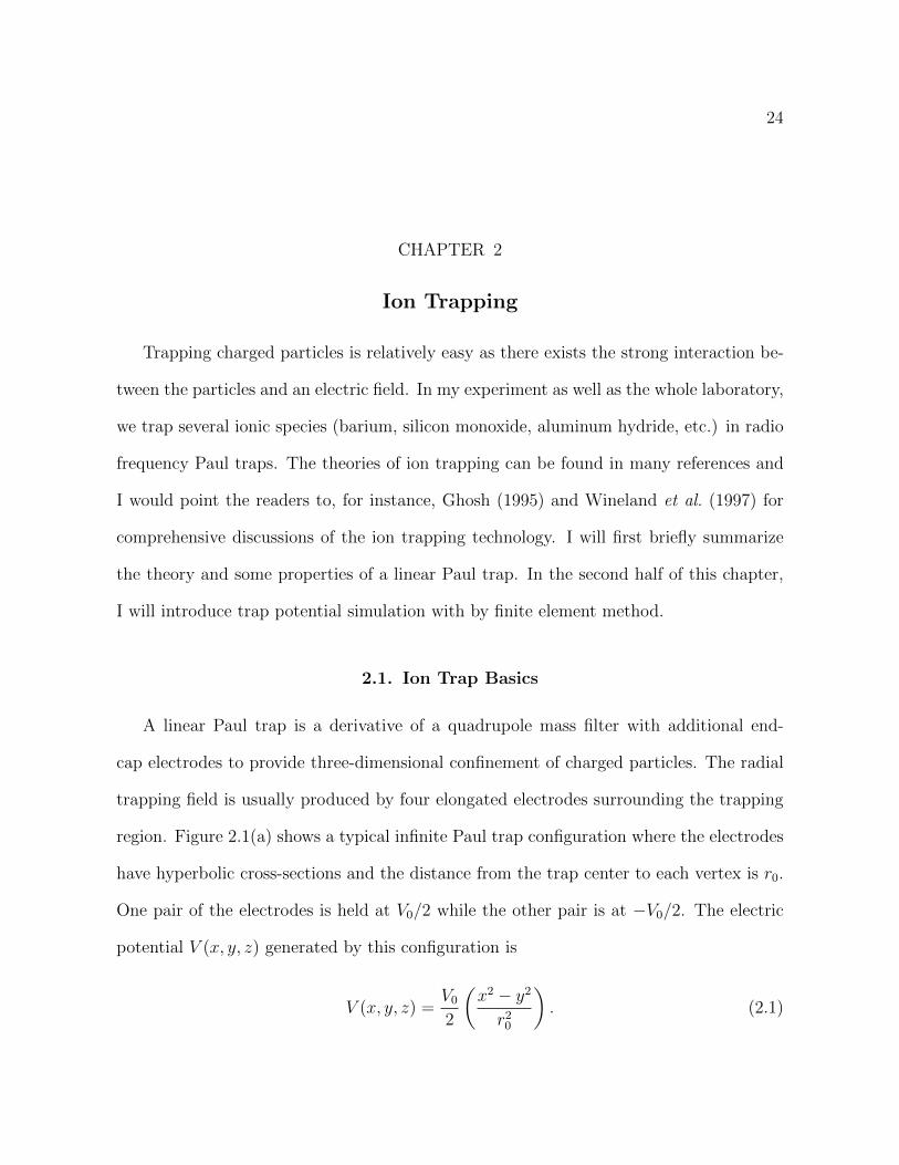
2.1. Ion Trap Basics
A linear Paul trap is a derivative of a quadrupole mass filter with additional end-
cap electrodes to provide three-dimensional confinement of charged particles. The radial
trapping field is usually produced by four elongated electrodes surrounding the trapping
region. Figure 2.1(a) shows a typical infinite Paul trap configuration where the electrodes
have hyperbolic cross-sections and the distance from the trap center to each vertex is r0.
One pair of the electrodes is held at V0/2 while the other pair is at V0/2. The electric
potential V (x, y, z) generated by this configuration is
V (x, y, z) =V0
2
x2 y2
r20
. (2.1)

25
x
y
r0
(a) (b)
Figure 2.1. Trap RF electrodes configuration
For a positive charge particle, the above potential is trapping in the x-direction but anti-
trapping in the y direction, which results in an unstable stationary line along z = 0 where
rV = ~E = 0. The electric potential cannot have any stable stationary point in free space
as it obeys the Laplace equation. The stationary point can be made stable when one
alternates the field polarity at an adequate frequency. Namely
V (x, y, z, t) =V0 cost
2
x2 y2
r20
is mechanically stable near z = 0 for properly chosen voltage amplitude V0 and oscillating
frequency . The parameter space of the AC field for stable trapping will be discussed
shortly. In practice, for trapping atomic or light molecular ions, the frequency of the AC
field falls into the radio frequency band while voltage up to 1000V can be generated by
a fairly simple circuitry.
Figure 2.1(b) shows the configuration commonly used in the lab where only one pair
of the electrodes is driven with the RF voltage Vrf. In addition, each pair of the electrodes
can be biased at a DC voltage Vdc1 and Vdc2. From Eq. (2.1) it is straightforward to find

26
the potential for this setup being
Vr
=Vdc1
2
1 x2 y2
r20
+
Vdc2 + Vrf cost
2
1 +
x2 y2
r20
(2.2)
=Vdc + Vrf cost
2
x2 y2
r20
+ V0
where Vdc = Vdc2 Vdc1 and V0 = (Vdc1 + Vdc2 + Vrf cost)/2. It is worth pointing out
that a none zero Vdc is necessary to break the degeneracy of radial motion.
The four-electrode setup does not confine particle axially. The axial, z-directional,
confinement is achieved by adding a pair of endcap electrodes to cap both ends of the
Paul trap. The endcaps produce the following potential:
Vz
= Vec
2z2 x2 y2
4z20
(2.3)
when the endcaps are separated by 2z0 and supplied at Vec.
The total potential of the trap is the sum of the fields due to all electrodes:
V = Vr
+ Vz
= V0 + Vx
x2 + Vy
y2 + Vz
z2 (2.4a)
where
Vx
= Vec
4z20 Vdc
2r20
+
Vrf
2r20cost (2.4b)
Vy
= Vec
4z20+
Vdc
2r20
Vrf
2r20cost (2.4c)
Vz
=Vec
2z20. (2.4d)

27
Note that Eq. (2.4) is only an approximation because Vr
and Vz
fulfill di↵erent bound-
ary conditions (as di↵erent electrodes are considered). In principle, one should solve
the Laplace equation with complete boundary conditions to obtain the total trapping
field. Numerical simulation of the trapping field will be discussed in the next section and
Appendix B.
Mathieu Equation
The motion of a particle of mass m and charge e in an electric field is governed by
m~r = e ~E(~r) = erV (~r). With the potential in Eq. (2.4), the equation of motion in each
direction is a Mathieu di↵erential equation:
d2x
d2+ (a
x
2qx
cos 2)x = 0 (2.5a)
d2y
d2+ (a
y
2qy
cos 2)y = 0 (2.5b)
d2z
d2+ (a
z
2qz
cos 2)z = 0 (2.5c)
with = t/2 being the canonical time and
ax
= 2eVec
mz202+
4eVdc
mr202, q
x
= 2eVrf
mr202, (2.6a)
ay
= 2eVec
mz202 4eVdc
mr202, q
y
=2eVrf
mr202, (2.6b)
az
=4eVec
mz202, q
z
= 0. (2.6c)

28
Figure 2.2. Stability diagram
Stability for One Ion
The Mathieu equation has either stable or unstable trajectories depending on the
values of the a and q parameters. Figure 2.2 shows the region where (a, q) exhibits stable
trajectories. Although there are multiple stable regions, usually an ion trap is operated
in the first stable region with a < q2 1.
The trap must be stable in all directions in order to trap an ion. Therefore, for a
given species, one must pick the RF voltage and frequency and the DC voltages carefully
to have the (a, q) pairs in the x, y, and z directions all falling into stable regions.
Motion of a Single Ion
In the z direction where q = 0 and a > 0, the trapped ion is a harmonic oscillator
z(t) = Az
cos(!z
t+ z
) (2.7)

29
where
!z
=paz
2=
seVec
mz20(2.8)
and Az
and z
are constants determined by the initial conditions.
For small, nonzero q, as in the radial direction, the solution to the Mathieu equation
is approximately
u(t) = A cos(!t+ ) (1 q
2cost). (2.9)
In the above equation, the cos!t term represents the secular oscillation at frequency
! =
ra+
q2
2
2(2.10)
while the cost term represents the so-called micromotion, which is the driven oscillation
due to the RF electric field. The micromotion amplitude is proportional to the secular
amplitude, and therefore, micromotion is vanished only if an ion has no secular motion.
In other words, micromotion always presents in thermal ions.
2.2. Trap Potential Simulation
A real life ion trap has complex geometry and thus would not produce an electric
potential as simple as Eqs. (2.1) and (2.3). Therefore, to understand the field provided
a practical trap, simulation is required. A common way to analyze an ion trap is by
simulating the dynamics of charged particles in the trap. For example, Tabor et al.
(2012) used SIMION to compute the ion trajectories in the traps and then extracted
some trap characteristics. On the other hand, the trap can be investigated by directly
solving the electric field according to the configuration.

30
The electric potential V of an ion trap is obtained by solving the Laplace’s equation
r2V (~r, t) = 0 (2.11)
with proper boundary conditions. The potential is time dependent since we are running a
radio frequency trap. However, the frequency is low enough such that the corresponding
propagation distance is much greater than the characteristic trap size; in other words, we
do not have to consider field retardation in an ion trap such that we can safely formulate
the problem as solving electrostatic potential. Assuming there are n boundaries =
1...n
(electrodes and all other conductors) in the trap, the potential can be written as
V (~r, t) =nX
i=1
i
Vi
(~r) (2.12)
where i
is the voltage supplied to each boundary i and can be either static of varying at
the radio frequency; Vi
is the solution of the Laplace’s equation with boundary i held at
unity and zero for all others:
r2Vi
(~r) = 0 (2.13a)
Vi
(~r) = 1,~r 2 i
(2.13b)
Vi
(~r) = 0,~r 2 i
. (2.13c)
I obtained the numerical solutions of each Vi
by the finite element method (FEM). There
are other numerical approaches developed exactly for the above problem, but the discus-
sion and comparison of other methods are beyond the scope of this work. Here, I just
point out that finite element method is more able to handle complex geometry than other

31
approaches such as finite di↵erence. Besides, there are some open source FEM packages
available, which makes this task more accessible.
Short Introduction to FEM
Regardless the mathematical framework, the idea of the finite element method is ac-
tually simple. The physical domain of the problem is first discretized into smaller regions,
usually tetrahedrals in the three dimensions and triangles in the two dimensions. Then we
can construct a basis function set i
over the domain. Among many fancy choices, the
basis function can simply be a piecewise linear function where it has unity value on one
vertex and zero elsewhere. These basis functions are called elements. Figure 2.3 shows an
example of the basis function in two dimensions. Any function f defined over the domain
can be approximated by
f(~r) =X
i
ci
i
(~r) (2.14)
where ci
are coecients that solve the Laplace equation r2f = 0. In the finite element
method, the di↵erential equations are solved in their weak form, i.e., if f is the solution,
thenZ
(r2f)g d~r = 0 (2.15)
orZrf ·rg d~r = 0 (2.16)
must be true for any test function g. From Eq. (2.15) to Eq. (2.16), I have applied the
rule of integration by parts. The required number of test functions g to completely define
the di↵erential equation in its weak form is exactly equal to the number of coecients ci
to be determined; that is the number of elements as well. Therefore, a natural choice of a

32
Figure 2.3. A sample basis function in the two dimensions.
set of g is the basis function set i
. For each g = j
, Eq. (2.16) yields a linear equation
of ci
:X
i
ci
Zr
i
·rj
d~r = 0 (2.17)
as eachR r
i
·rj
d~r hri
,rj
i pair can be evaluated beforehand. Note that some of
the ci
in each linear equation are pre-determined by the boundary conditions and therefore
the number of unknown variables are reduced. Finally, the Laplace equation is formulated
into a large system of linear equations. It is worth pointing out that, as i
is compact,
hri
,rj
i is zero when i is far from j, and therefore the linear system is sparse. There
are many numerical methods for solving sparse linear systems in quick and accurate ways,
which makes finite element analysis powerful for a large domain size. Here, I however will
not discuss the actual numerical schemes used in my simulation since it is beyond the
scope of this thesis.
Implementation
In my work, the discretization of the trap geometry was done with Gmsh (v2.12),
and the finite element analysis was done with Freefem++ (v3.42). One should refer to

33
the manuals for software usage, but the scripts for this work will be provided later in
Appendix B.
Here I present the simulation result for the single ion trap as an example. The full
design of the trap will be described in Section 3.1, but in the simulation, it is simplified
to four long rods for the RF and two short pins for end caps. The setup is enclosed in a
cylindrical grounding can for the computational purpose. The size of the enclosure should
be large enough so its boundary e↵ect does not significantly alter the simulation result
in the trap region. The upper two drawings in Fig. 2.4 show the configuration rendered
in Gmsh viewing along the z- and the x-axis; so are the bottom two, with the surfaces
of the electrodes meshed. In this example, the free space region for the electric potential
is split into 7.6 105 tetrahedrons, and all the surfaces of the electrodes are discretized
into 9.7 104 triangles. This mesh ensemble is formed by 1.4 105 vertices, which are
the variables for solving the Laplace equation.
After the trap geometry has been meshed, I used Freefem++ to solve the Laplace
equation. As mentioned earlier, the solver is invoked several times for various boundary
conditions settings. In this example, boundaries are divided into four groups: (1) one
diagonal pair of the RF rods, (2) the other diagonal pair of the RF rods, (3) the endcap
electrodes, and (4) the grounding cylinder. Solutions to the cases where (1), (2), and
(3) each being held at unity voltage were computed. With these simulation results, the
electric potential produced by this trap can be reconstructed with the basis function set.
Post-processing
Because the domain can not be discretized based on a regular grid, the simulation
result is in fact a list of scattered data points. To better understand the result, the

34
Z X
Y
ZX
Y
Z X
Y
ZX
Y
Figure 2.4. The trap geometry set up for the FEM simulation. Top: inputgeometry. Bottom: the mesh.
multipole expansion is applied to the simulated field:
V (~r) = V (r, ,) =X
l
X
m
Clm
m
l
(r, ,) (2.18)
=X
l
X
m
Clm
rlPm
l
(cos )
8>><
>>:
cos(m) for m 0
sin(m) for m < 0

35
where Pm
l
is the associated Legender polynomial, commonly used in solving the Laplace
equation with a cylindrical symmetry. Note that in the above expansion, all the odd l and
odd m terms are automatically dropped due to additional symmetry set by the boundary
conditions. In contrast, one should include all terms if no specific symmetry condition
exists.
The lowest order (l = 0 and m = 0) in the expansion represents a constant potential.
There are three terms for l = 2:
02 = r2P 0
2 (cos ) =1
2(3 cos2 1) =
1
2(x2 y2 + 2z2) for m = 0, (2.19a)
22 = r2P 2
2 (cos ) cos(2) = 3(cos2 1) cos(2) = 3(x2 y2) for m = 2, (2.19b)
and
22 = r2P2
2 (cos ) sin(2) = 18(cos2 1) sin(2) =
1
4xy for m = 2. (2.19c)
These potential forms represent the three mutually di↵erent quadratic fields. In fact,
Eq. (2.19a) is the lowest order harmonic potential from the end caps. Equation (2.19b) is
the potential for ideal the infinit linear quadruple Paul trap; so is Eq. (2.19c) but with the
trap rotated by 45 degrees. Refer to previous section. See Table 2.1 for the visualization
of the potential fields in Eq. (2.19) as well as those up to l = 8.

36
Table 2.1. The visualizations and the representations of m
l
for l 8.
l m xy (z = 0) xz (y = 0) m
l
0 0 1
2 0 12 (x2 y2 + 2z2)
2 2 3 (x2 y2)
2 -2 14xy
4 0 18 (3r
4 30r2z2 + 35z4)
4 2 52 (r
2 7z2) 22
4 -2 16 (7z
2 r2) 22
4 4 105 (x4 6x2y2 + y4)
4 -4 196xy (y
2 x2)
6 0 116 (5r6 + 105r4z2 315r2z4 + 231z6)
6 2 358 (r4 18r2z2 + 33z4) 2
2

37
Table 2.1 (continued)
l m xy (z = 0) xz (y = 0) m
l
6 -2 116 (r
4 18r2z2 + 33z4) 22
6 4 92 (r
2 11z2) 44
6 -4 110 (11z
2 r2) 44
6 6 10395 (x6 15x4y2 + 15x2y4 y6)
6 -6 123040 (3x5y + 10x3y3 3xy5)
8 0 1128 (35r
8 1260r6z2 + 6930r4z4 12012r2z6 + 6435z8)
8 2 10516 (r6 33r4z2 + 143r2z4 143z6) 2
2
8 -2 132 (r6 + 33r4z2 143r2z4 + 143z6) 2
2
8 4 998 (r4 26r2z2 + 65z4) 4
4
8 -4 140 (r
4 26r2z2 + 65z4) 44
8 6 132 (r2 15z2) 6
6

38
Table 2.1 (continued)
l m xy (z = 0) xz (y = 0) m
l
8 -6 114 (15z
2 r2) 66
8 8 2027025 (x8 28x6y2 + 70x4y4 28x2y6 + y8)
8 -8 11290240 (x7y + 7x5y3 7x3y5 + xy7)
The expansion coecients are obtained by fitting the simulation data to Eq. (2.18)
with a cuto↵ lmax
. Because the nature of this expansion is a linear combination of or-
thogonal functions, the least square fitting will work nicely. Refer to Appendix B for the
python implementation. Table 2.2 summarizes the fitting result for the single ion trap.
Geometric Factor
The geometric factor is used to compare the l = 2 quadrupole field produced by a
practical trap design to the one of the ideal design with the same electrode spacing. For
instance, from Eq. (2.1), the potential field in an ideal linear Paul trap has the following
form
V0
2
x2 y2
r20,
where V0 is the voltage applied to the electrodes and r0 is the shortest distance from the
trap center to the electrodes. The geometric factor r
is then obtained by comparing
the above equation (with V0 = 1) to the corresponding (l,m) = (2, 2) term from the

39
expansion:
r
2r20
x2 y2
= C2
222 = C2
2 3x2 y2
. (2.20)
Table 2.2. The coecients of the multipole expansion in Eq. (2.18) with acuto↵ at l = 8. In B1, RF electrodes in the (+x,+y) and (-x,-y) quadrantsare held at 1 while all other boundaries are at zero. In B2, RF electrodesin the (-x,+y) and (+x,-y) quandatnts are charged. In B3, the endcapelectrodes are charged. In this simulation and analysis, the length unit ismm. Only those points within
px2 + y2 < 0.2mm and |z| < 0.8mm are
included in the fitting.
l m B1: RF-1 B2: RF-2 B3: Endcaps
0 0 4.83 101 4.83 101 2.87 102
2 0 1.50 101 1.49 101 3.01 101
2 2 1.35 104 4.05 105 1.17 104
2 -2 1.86 101 1.86 101 6.04 103
4 0 2.17 101 2.24 101 4.43 101
4 2 2.81 104 5.15 104 2.45 104
4 -2 1.69 1.46 2.29 101
4 4 1.07 103 1.22 103 8.97 104
4 -4 2.45 101 1.07 1.606 0 2.92 101 2.80 101 5.75 101
6 2 3.53 104 5.37 104 1.89 104
6 -2 1.19 101 1.08 101 1.126 4 1.58 104 3.26 104 4.83 104
6 -4 9.96 101 5.62 101 4.41 101
6 6 3.73 105 3.64 105 8.50 107
6 -6 1.12 105 1.02 105 1.06 104
8 0 4.97 103 2.65 103 2.28 103
8 2 1.44 104 2.04 104 6.06 105
8 -2 2.79 101 2.65 101 1.408 4 1.10 105 2.35 105 1.23 105
8 -4 2.53 102 9.28 101 1.61 102
8 6 2.26 106 2.95 106 6.68 107
8 -6 1.30 105 1.52 105 2.14 104
8 8 5.75 106 1.48 105 8.90 106
8 -8 3.48 108 2.66 108 8.13 107
40
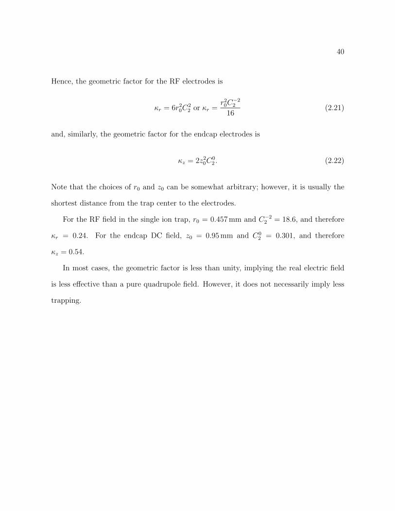
Hence, the geometric factor for the RF electrodes is
r
= 6r20C22 or
r
=r20C
22
16(2.21)
and, similarly, the geometric factor for the endcap electrodes is
z
= 2z20C02 . (2.22)
Note that the choices of r0 and z0 can be somewhat arbitrary; however, it is usually the
shortest distance from the trap center to the electrodes.
For the RF field in the single ion trap, r0 = 0.457mm and C22 = 18.6, and therefore
r
= 0.24. For the endcap DC field, z0 = 0.95mm and C02 = 0.301, and therefore
z
= 0.54.
In most cases, the geometric factor is less than unity, implying the real electric field
is less e↵ective than a pure quadrupole field. However, it does not necessarily imply less
trapping.

41
CHAPTER 3
Apparatus for the Single Ion Trap
The single ion trap is the house for the single ion precision spectroscopy experiment.
This chapter introduces the apparatus for the experiment with a single trapped barium
ion.
3.1. The Single Ion Trap
This trap is designed to trap ions in the Lamb-Dicke regime such that we can drive
sideband transitions to perform motional quantum state manipulation such as ground
state cooling. Typically, the value of the Lamb-Dicke parameter is set to about 0.1. To
build a trap for a single 138Ba+ in this regime, we first determine the secular frequency
needed. The Lamb-Dicke parameter is the ratio between the ground state wavefunction
extent a0 and the transition wavelength . For 0.1 and 1000 nm for a typical
optical transition, the wavefunction spread a0 is of order 30 nm. As a0 = (2h/m!)1/2, the
trap secular frequency ! is then of order 2 1MHz for the barium ion.
The motional quantum state manipulation is usually performed in the axial mode
along which micromotion is minimal. From Eq. (2.8) we have
Vec
z20=
!2z
m
ez
= 2.8 102 [V/mm2]
for !z
= 2 1MHz and assuming z
= 0.2. Therefore, if we supply up to 1000V to the
endcaps, the separation between the two electrodes is of order millimeters.

42
The radial part of the trap is designed in a similar manner. Assuming there is no
DC field in the radial direction, from Eq. (2.10) the radial secular frequency is then
!r
= qr
/2p2 where is the RF drive frequency and q
r
is either qx
or qy
. That is
Vrf
r20=
p2m!
r
e
when the radial geometric factor is unity. We would like to keep the radial secular fre-
quencies higher than the axial secular frequency so the axial secular motion is less likely
to resonant, either directly or parametrically, with the radial modes. Also, in the single
ion precision spectroscopy experiment, where a spectroscopy ion is co-trapped with a logic
ion, the two-ion ensemble can be kept aligned to the axis to minimize RF micromotions.
We chose the radial secular frequency to be twice of the axial one. Since the secular
motion approximation in Eq. (2.9) is valid when the RF drive frequency is much higher
than the secular frequency, we set the RF frequency to be at least 10 times of the radial
frequency. For example, with !r
= 2 2MHz, = 2 20MHz, and Vrf up to several
hundred volts, the trap’s radial size r0 is 1mm or so.
Geometry
The outline of the single ion trap is illustrated in Fig. 3.1. The RF field is provided by
four rod electrodes, and the axial confinement is provided by two endcap pins installed
on the trap axis. Due to the RF circuit configuration (see page 48), the RF electrodes
can not be DC biased individually. Therefore, there are additional four rod electrodes
surrounding the trap, similar to the RF electrodes, to provide DC electric field in the
radial direction.

43
Figure 3.1. Single ion trap outline
The RF electrodes have a 0.686mm diameter and are made of tungsten. They are
evenly distributed over a circle of 0.8mm radius; r0 is 0.457mm. The DC bias electrodes
have a 1.27mm diameter and are made of stainless steel. They are located on a circle of
3.18mm radius, directly behind the RF electrodes. The endcap electrodes are made of
the 0.686mm tungsten wire as well. The two endcaps are separated by 2z0 = 1.9mm.
This configuration is simulated and analyzed by the procedure in Section 2.2, from which
the geometric factors r
= 0.24 and z
= 0.54 are obtained.
Trap Electrodes
Although an ion trap acts like a capacitor and there is no current flowing between the
electrodes via free space, charges are constantly redistributing on the electrode surfaces
when the trap is driven with RF signal. Known as the skin e↵ect, the AC field propagates
near the surface in a conductor. Therefore the AC conductivity can be significantly worse
than the DC conductivity, and the area around the trap electrodes can accumulate lots of
heat as heat dissipation is extremely slow in the vacuum. The skin depth of a conductor

44
Table 3.1. Skin depth and AC resistance
MaterialResistivity Relt. permeability Skin depth (µm)
(m) µr
= µ/µ0 1MHz 3MHz 10MHz
Aluminum 2.65 108 1 81.9 47.3 25.9Copper 1.69 108 1 65.4 37.8 20.7Nickel 6.9 108 200 9.3 5.4 3.0numlver 1.63 108 1 64.3 37.1 20.3
Stainless steel 300 7 107 1 421 243 133Tungsten 5.4 108 1 117 68 37
is approximately
=p2µ (3.1)
where is the DC resistivity, µ is the permeability, and is the AC angular frequency.
For a rod electrode of radius r, the AC resistance per axial unit length is
R
2r(3.2)
when the rod thickness is much greater than the skin depth. Table 3.1 lists the skin depth
for some common materials. In particular, when driven at around 20MHz, the skin depth
of the tungsten electrodes is around 25 µm, fraction of the physical radius. Hence, the
conduction of charges on the electrodes is limited by the skin e↵ect but not the physical
cross-section of the rod.
Tungsten is chosen over stainless steel because of its better AC conductivity. As
aluminum and copper are softer than tungsten, building a millimeter scale ion trap with
tungsten may be easier. Silver has the best conductivity among the common materials
in Table 3.1; in the future, one can consider plating the electrode with silver to further
reduce the resistance.

45
electrode (anode)
SS cylinder (cathode)
1% KOH
(top view) (side view)
Figure 3.2. Tungsten wire electropolishing
All the electrodes were fabricated from stocked materials. They were trimmed, etched,
and polished in house. For small diameter, both stainless steel rods and tungsten rods are
fairly easy to handle in the laboratory. These electrodes were first cut o↵ from a longer raw
piece. They were trimmed to the desired length with Dremel cutting and grinding discs.
Oxygen-free copper (OFHC) wires were bonded to each electrode by silver brazing for
connecting to the external DC/RF circuitries. Lastly, the electrodes were electropolished
before assembled with other parts.
Electropolishing
Electropolishing is a polishing process utilizing electrolysis. It uses ions in the aqueous
solution to remove roughness on a conducting surface, where field emission is more likely to
take place when driving at a higher voltage. There were also studies showing a polished
trap has a lower motional heating rate, which is crucial for motional quantum state
manipulation.
Di↵erent metals require di↵erent recipes for electropolishing. For tungsten, I followed
the instruction by Latawiec and Lockwood (1966); Hunt (1976). As illustrated in Fig. 3.2,
the tungsten rod electrode (anode) and a stainless steel tube (cathode) are set up coaxially

46
in the 1% potassium hydroxide (KOH) solution. One of the keys to successful electropol-
ishing is to have a uniform electric field density. For cylindrical objects, this is achieved
by using a cathode tube which has a large inner diameter and is longer than the rod to be
polished. The inner diameter of the tube I used is around 50mm. Good electropolishing
also requires right current density as well as the application time. The reference provided
a suggestion to the voltage and the reaction time as a starting point; however, these pa-
rameters require further experiment. Usually, the tungsten parts are found grayish before
any surface treatment. While electropolishing removes the surface roughness as well as
contamination, polished tungsten part shows a shining surface. Unfortunately, we did
not have any equipment to further exam the surface. Empirically, I found insucient
and rushed electropolishing would both result in a fuzzy and darkish surface, and usually
optimizing the electrolysis voltage would make an improvement.
For parts with complicated geometry, professional electropolishing services such as
Abel Electropolishing (Chicago, IL) should be considered.
Macro Electrode Mount
The trap electrodes are held by four macro stands, see Fig. 3.3. Macro is a machinable
ceramic material; it is compatible with the ultra-high vacuum. The DC resistivity is
1017 cm. While high voltages are supplied to the trap, it is necessary to check for
Macro’s dielectric breakdown. The DC threshold is 129 kV/mm, and the AC threshold is
45 kV/mm. In this trap, the gap between the RF electrodes to the endcap electrodes is
the smallest, approximately 0.11mm. Assuming the voltage di↵erence between electrodes
is 1000V, the electric field is then approximately 9 kV/mm, which is well below both the
AC and DC breakdown threshold.

47
(a) (b)
Figure 3.3. Trap assembly
The outline of the macro stands are shown in Figs. C.1 to C.3.
Trap Assembly
The trap was assembled onto a base plate first, and then the whole assembly was
mounted inside a 6” octagon vacuum chamber (Kimball Physics MCF600-SphOct-F2C8).
Electrical connections are established by bare oxygen-free copper wires as mentioned
earlier. Both the pushpin connectors and the barrel connectors (both from Kurt J. Lesker)
were used to join wires to the feedthroughs. Each diagonal pair of the RF electrodes were
internally connected, thus there are two lines for the RF; they are connected to an RF
feedthrough. All the other DC electrodes (two endcapes and four biasing electrodes) are
connected to another vacuum electrical feedthrough.
The partially assembled trap is shown in Fig. 3.3. After other trap accessories such as
the oven are installed inside, the vacuum chamber is evacuated and sealed.

48
3.2. Trap Electrical
RF Source
The operation of an ion trap requires several hundred volts on the RF electrodes
to keep a single barium ion with suciently radial confinement. Such high RF voltage
is usually achieved by using a resonator with a high quality-factor. Most ion trapping
laboratories use a coaxial resonator for this purpose.
The idea of using a coaxial resonator to produce the high RF voltage is to have a
quarter-wave resonance and the load that requires a high RF voltage is attached to the
anti-node (at the quarter-wave location). In a coaxial resonator, one end of the core is
short to the ground while the other end remains open and is connected to the RF elec-
trodes. This configuration forms a quarter-wave resonance because, when on resonance,
the RF electromagnetic field across the resonator is exactly 1/4 of the wavelength (Viz-
muller, 1995). The simplest form of a coaxial resonator is a straight inner conductor
inside a cylindrical shell ground and the length of the resonator is quarter wavelength.
This design is then unpractical for 25MHz RF as the wavelength is 12m. However, by
introducing a helical inner conductor, the group velocity of the electromagnetic wave is
much slower and hence significantly reduces the resonator’s dimensions (Zverev, 1967).
Some empirical design equations for helical resonators can be found in Macalpine and
Schildknecht (1959) and was employed when building the resonator for this single ion
trap. Refer to Fig. 3.4 for the outline of the helical resonator. Although there are several
dimensions in the resonator, one only needs to choose the resonance frequency fe
and the
diameter of the shield D. Other parameters such as resonator length B, wire gauge d0,

49
Figure 3.4. Outline of a helical resonator. (From Macalpine and Schild-knecht (1959, Fig. 2))
helix radius d and pitch are determined automatically by either physics laws or optimized
conditions found empirically. However, note that the resonance of a helical resonator will
be shifted when an additional capacitance is loaded. In practice, one anticipates 5 to
10 pF each from the trap and other circuit components such as cables and connectors; the
capacitance of our helical resonator is estimated to be around 5 pF. Therefore, the loaded
resonant frequency is expected to lower by about 1/2 as the resonance goes inversely as
the square root of capacitance.

50
Figure 3.5. Helical resonator design chart. (From (Macalpine and Schild-knecht, 1959, Fig. 4))
In light of the shift, I designed this helical resonator to have unloaded resonant fre-
quency fe
= 50MHz with a 109.2mm inner diameter ground shield. By using the chart
in Fig. 3.5, the helical coil is found to have N = 9 turns with = 9.4mm pitch. The coil
diameter d is 61mm based on the optimized condition d/D = 0.55. The wire gauge d0 is
1/8” (3.175mm), much greater than the skin depth (around 10 µm in 10 to 100MHz) of
the RF electric field to have low loss. Both the coil and the shield are oxygen-free copper.
Note that the design of the helical resonator is not unique, but is constrained by practical
issues. For instance, we constructed the coil from a 72”-long (1.8m) copper rod. This
rod was the longest piece we could easily obtain and was just long enough to build the

51
(a) inner coil (b) resonator
Figure 3.6. The helical resonator used to drive the single ion trap.
coil. In terms of the rod diameter, a thicker rod is harder to wind into a coil; a thinner
rod will result in a springy coil which hurts the resonator’s stability.
Additional two copper end caps are added to the ground can to better shield the RF
field in the resonator. The open end of the core conductor is directly attached to the
vacuum feedthrough to delivery RF to the trap. I found that using extra cables and
common RF connectors adversely degrades the resonance quality factor and stability.
Proper grounding of the resonator is crucial to the stability as well. I used a stainless
steel grounding braid to connect the ground can to the optical table.
The energy is coupled into the circuit by magnetic induction; see Fig. 3.7 for the
schematic. The coupling coil is a single loop magnet wire of which the diameter is slightly
smaller than the one of the resonator’s helical coil. The loop is aligned to the resonator’s
coil coaxially; the location was adjusted for optimal coupling. The primary circuit (i.e.,
the coupling loop) has a bi-directional coupler that samples 20 dB of the RF power trav-
eling forward and backward. The RF traveling forward carries the power pumping the

52
AMP CPL
FDBD
(a) circuit
0
0.02
0.04
0.06
0.08
0.1
0.12
0.14
0.16
23 23.1 23.2 23.3 23.4 23.5 23.6 23.7 23.8 23.9 24
Refle
ctiv
e po
wer
(ar
b. u
nit)
Drive frequency (MHz)
Trap resonance: Resonance_scan_20110802.txt
Res. freq. = 23.399 MHzFull width = 0.057 MHzQ = 414
(b) resonance
Figure 3.7. RF resonant circuit with a helical resonator
resonator, and the RF not coupled into the resonator travels backward. The RF resonant
circuit is optimized by tuning the drive frequency and the location of the coupling loop
such that the reflective RF is minimized. Figure 3.7(b) is a typical spectrum of the loaded
resonator. A resonance is found at 23.5MHz with a linewidth of 60 kHz. The Q factor is
400, while the unloaded Q factor is around 1500.
The pump source is generated by a signal generator followed by an RF amplifier with
approximately 40 dB gain. The RF source with up to 37 dBm power drives the primary
coupling coil directly. Figure 3.8 shows the output voltage at di↵erent pump power. The
output voltage is measured at the feedthrough conductor, which is the closest test point to
the trap electrodes. Although the measurement is done with a high impedance oscilloscope

53
0
500
1000
1500
2000
2500
3000
3500
4000
-30 -25 -20 -15 -10 -5
Trap
rf
peak
-to-
peak
vol
tage
(V)
Power set on function generator (dBm)
High voltage calibration 2011-07-29
Figure 3.8. RF voltage calibration
probe, the circuit is still perturbed such that the resonance is shifted. However, the quality
factor lowers only slightly, thus this calibration should be representative. The peak-to-
peak RF voltage is around 3500V when the circuit is resonantly pumped by 37 dBm.
Note that the above calibrations were performed with the trap in vacuum condition.
In particular, when the trap chamber’s pressure is of order 1Torr, the RF electric field
generated by this system is able to cause vacuum arc.
In passing, Siverns et al. (2012) provides another example of using a helical resonator
for driving the ion trap.
DC Controls
The DC voltages for the endcaps and the biasing electrodes are each provided by a high
voltage regulation circuit outlined in Fig. 3.9. The circuit uses a two-stage amplification
structure: field-e↵ect transition Q1 forms a common source amplifier stage and Q2 forms
a common drain stage (Horowitz et al., 1980).

54
Figure 3.9. High voltage regulator
A low-pass filter is added in between each DC electrode and its voltage source to
stabilize the DC voltage on the electrode. As illustrated in Fig. 3.10, the filters also
prevent the RF power, capacitively picked up by the DC electrodes, traveling backward
and perturbing the DC supplies. The single ion trapping system uses a simple low-pass RC
filter. The resistor is 50 k and the capacitors are 22 µF, which results in the 3 dB cuto↵
frequency to be 0.14Hz; at the RF drive frequency = 2 24MHz, the attenuation is
82 dB.
The resistor in this low-pass filter can be replaced by an inductor. The revised version
is called a -filter, which is commonly used in RF electronics for its low impedance.
However, as there is no DC current flowing between the voltage source and the electrodes,
one can use either version of the filter circuit.

55
V C
R
C
EC
RF-trap
Figure 3.10. The DC low-pass filtering circuit. V: DC voltage supply. C:22 µF capacitor. R: 50 k resistor. EC: endcap electrode. RF-trap: nearbyRF electrodes. The box indicates the filter box.
3.3. Barium Oven
barium ions are loaded into the trap by photoionization. A neutral barium flux is
generated by the barium oven, and then the neutral barium is ionization inside the trap.
The oven is an alumina tube with one end fused and wrapped by a tungsten heating
filament. See Fig. 3.11. It is attached to a vacuum electrical feedthrough directly to
form a single assembly. This particular feedthrough is dedicated for the oven for easy
transportation. Because the tungsten filament is rigid enough, the oven is only held
be the tungsten coil whose two ends were spot-welded onto the feedthrough conductors.
However, when heated up, thermal expansion may deform the coil and shifts the oven’s
position. Therefore, it takes some practice and attempts to build a satisfactory oven
assembly.
Inside the chamber, the oven is aligned vertically, about 25mm directly below the
trapping region. While the oven output flux is expected to be quite diverging, I used two
apertures to produce a somewhat collimated atomic beam pointing toward the trap. In
practice, the two apertures were installed beforehand during the trapping assembling to
ensure good alignment, see Fig. 3.11(b).

56
(a) (b)
Figure 3.11. (a) Alumina tubing with tungsten coil as the barium oven. (b)The apertures for the oven output.
To fill the oven, barium is chopped into smaller pieces to fit it the tube. Since barium
is quite reactive, the oven preparation was done in a nitrogen-filled glove box to slow down
oxidization. After the oven was prepared, it was installed onto the vacuum chamber within
the shortest possible time; the chamber was pumped down right after the installation.
The heating filament is usually driven at 1.2A, which would make the tungsten coil
glowing.
Photoionization will be discussed in Section 4.1. Ablation loading, a di↵erent loading
strategy which does not require an oven, will be discussed in Section 7.1.
3.4. Laser Systems
The single ion experiment used four lasers: two (791 nm and 337 nm) for the photoion-
ization loading of barium, and two (493 nm and 650 nm) for the Doppler laser cooling and
internal state manipulation.

57
The 493 nm laser drives the 6S1/2 ! 6P1/2 transition in Ba+. It is an integrated
Toptica DL-Pro laser system with an IR laser diode at 987 nm pumping a cavity-enhanced
second harmonic generation module. The frequency doubling involves the noncritical
phase matching (NCPM) with a potassium niobate (KNbO3) crystal. This SHG process
is tuned by the crystal’s temperature and is optimized at 40 C with 80mW output
power.
The 650 nm laser, which drives the 5D3/2 ! 6P1/2 transition in Ba+, is a DL-100
module with 20mW output power. Part of the ECDL output is used to injection lock
a slave diode laser, which provides more 650 nm laser power. Injection locking uses the
master laser to force the slave laser’s cavity resonating at the same mode. This is done by
counter-propagating the master laser against the slave laser’s output such that the master
laser’s field is injected into the slave laser’s gain medium. In this project, the slave laser
diode has an anti-reflection coating such that there is an insucient reflection to form the
laser cavity used to establish stable laser mode internally. In general, non-AR-coated laser
diode would work equally fine, but with a smaller capture range for locking. Injection
locking is confirmed by inspecting the slave laser’s spectrum on a scanning Fabry-Perot
interferometer.
The 791 nm laser is a DL-Pro module; it couples the 6s2 1S0 and the 6s6 3P1 states in
neutral barium atoms as the first step of the photoionization. The nitrogen laser, a pulsed
ultra-violate (337 nm) gas laser, further ionizes the excited population to form Ba+. The
N2 laser is a Stanford Research System NL100.

58
3.5. Laser Stabilization
The wavelength of an ECDL is controlled by the driving current, the operating temper-
ature, and the piezo’s thickness (which is set by its applied voltage). These parameters are
sensitive to the environment’s perturbation and thus need to be regulated. Furthermore,
the laser’s driving parameters are modulated to actively stabilize the output frequency.
Laser frequency stabilization involves frequency (or wavelength) measurement and
error-correcting feedback. In the lab, we routinely stabilize lasers through directly wave-
length measurement by a wavelength meter. This approach is quick and least involving
but has slow feedback bandwidth and less accurate. Detail follows.
Stabilizing lasers by a wavelength meter is straightforward. In the lab, we measure
the laser frequency by the HighFiness WSU-2 optical wavelength meter which has a
2MHz short-term resolution. Over a longer time scale, the measurement result is highly
correlated to the environmental parameters such as ambient temperature and atmospheric
pressure. Therefore, we periodically calibrate our wavelength meter with a stabilized
Helium-Neon laser (Research Electro-Optics, Inc.) which provides ±3MHz stability over
several hours.
In order to stabilize multiple lasers, laser beams are combined via polarizing or dichroic
beam splitters before coupling into the wavemeter. As measurement can be performed for
only one laser each time, we put each sample beam through an acoustic-optical modulator
and program these AOM switches to rotate the measurement. A computer controls the
measurement sequences, captures the result, and generates the feedback signals at a Na-
tional Instruments analog output card. In practice, the repetition time for the feedback is

59
Figure 3.12. Drift of the wavelength meter locking mechanism.
of order 100ms for each laser. Currently, there are up to 5 lasers locked to the wavemeter
and the feedback bandwidth is 2 to 3Hz.
The performance of our wavemeter locking is tested by performing laser induced flu-
orescence spectroscopy with Ba+. Refer to Section 4.2 for details of Ba+ spectroscopy;
in short, the fluorescence from a single barium ion is monitored for around 20 hours. If
the excitation laser frequency changes, then the fluorescence changes as well. In this test,
only the relevant lasers, the 493 nm and the 650 nm lasers, are stabilized to the wave-
length meter; the wavemeter is calibrated to the stabilized He-Ne laser every 30 minutes.
In Fig. 3.12, I plot the fluorescence count at di↵erent laser detuning added by an AOM.
In the plot, the contour that yields a constant fluorescence count is then a measurement
of the laser frequency drift over time. The vertical dashed lines mark the periodic He-Ne

60
calibration and are often found to coincide big jumps in the drift. Overall speaking, our
wavemeter locking mechanism is able to keep lasers stabilized to ±10MHz within a day
with frequent calibration to the He-Ne laser. Without calibration, the wavemeter can
quickly drift away within an hour.
3.6. Fluorescence Detection
We detected the barium ion with its fluorescence. With ecient laser cooling, trapped
ions can be highly localized such that the fluorescence is like a point light source, which
can be imaged by microscope setup. When Coulomb crystal is formed, the typical spacing
between localized ions is of order 10 µm. While the size of the camera sensor pixels is also
around 10 µm, approximately 10 times optical magnification in the imaging system would
be sucient to resolve single ions on the camera.
The outline of the optical system for collecting barium fluorescence is depicted in
Fig. 3.13. Like common microscopy design, the imaging system has three major parts:
the objective lens, the relay lens, and the tube lens. The objective collects light from
the object and the tube lens focuses the light onto the camera sensor for forming the
image. While we adopt the infinity corrected configuration where the rays are collimated
in between the objective and the tube lens, the separation between these two optics
becomes an independent parameter. In addition, a relay lens, which is like a Galilean
telescope, can be inserted to provide additional magnification.
In this setup for imaging a single ion, the objective lens is a 2”-diameter aspheric
lens with a 40mm focal length. The relay optical system is a Galilean telescope made
of an f = 100mm and an f = 30mm achromatic doublet lens, which provides 3.33X

61
ThorlabsAL5040f=40mm,Aspheric2" dia
ThorlabsAC508-100f=100mm,Achromatic doublet2" dia
ThorlabsAC254-030f=30mm,Achromatic doublet1" dia
ThorlabsAC254-150f=150mm,Achromatic doublet1" dia
Iris Diaphragm
ThorlabsDMSP805Shortpass filter at 805nm1" dia
ThorlabsBB1-E03PBackside polished1" dia
Andor CCD
L-bracket for mountingontranslation stagte
Cube for connection PMT
Figure 3.13. Imaging optics for the single ion experiment.
magnification. Inside the relay optics, a small iris is placed at the internal focal plane
for blocking stray light. This approach is like setting an entrance pupil at the object and
has significantly reduced the level of background scattered light. An optical bandpass
filter is attached to the relay lens to transmit photon with a wavelength around 493 nm,
corresponding to the 6S1/2 ! 6P1/2 transition in Ba+. The transmission is further split
evenly by a non-polarising beam splitter. Half of the light (the reflection of the NPBS) is
sent to a photomultiplier tube (PMT) for photon counting purpose; rest of the light (the
transmission of the NPBS) is focused by the tube lens, an f = 150mm achromatic doublet
lens, to form the image on an electron multiplying CCD (Andor Luca-R EMCCD). The
overall magnification of this imaging system is 12.5X.
The trap electrodes partially block the ion’s fluorescence. Treat the single ion as a
point source, the solid angle of the emission is reduced to 0.56 sr, which is equivalent to

62
4.4% of the total fluorescence. The objective lens has a 0.98 sr solid angle, greater than the
emission solid angle. Rest of the optics in the imaging system all have sucient aperture
sizes for light propagation. By taking the transmission of each optics into account, the
collection eciency is reduced to approximately 1%. However, due to optical aberration,
the clear aperture of this system is, in fact, smaller for imaging, which would lower the
collection eciency roughly by 10. See Section 6.3 for more discussion and analysis.
Fortunately, photon counting is immune to aberration, thus the eciency is not a↵ected.
The total eciency, due to the detector, signal amplifier, and the discriminator, is about
10%. Therefore, the overall photon counting eciency is around 103, which is equivalent
to a maximum photon flux of 105/s.

63
CHAPTER 4
Single Ion Experiments
Figure 4.1. A trapped single Ba+ was first observed in the single ion trapat around 2pm on September 2, 2011.
This chapter discusses the operation of the single ion trap. First, a summary of this
trap’s physical properties follows.
• r0 = 0.457mm and r
= 0.24.
• z0 = 0.95mm and z
= 0.54.
• The trap is driven at = 2 23.5MHz.
Fig. 4.2 shows the theoretical region of the RF voltage Vrf and the endcap voltage Vec for
stable trapping. It also shows the expected secular frequencies. As mentioned earlier, we
operate around !z
= 2 1MHz and !x,y
2 2MHz.

64
0
200
400
600
800
1000
1200
1400
0 50 100 150 200 250 300 350 400 450 500
Min
imum
RF
Volta
ge (
V)
DC Voltage (V)
Trap Stable Region f=23.5MHz
Figure 4.2. Stability region for Vrf and Vec.
4.1. Loading an Ion
A single barium ion is loaded into the trap by photoionization where a first photon
resonantly excites a neutral barium atom into an immediate excitation state, and a second
photon subsequently drives the excited atom to its ionization continuum. This process is
called the resonance enhanced multi-photon ionization or REMPI.
For loading barium ions, there are two convenient intermediate states one can use:
5d6p 3D1 and 6s6p 3P1. Excitation to 5d6p 3D1 requires a 413 nm photon from the ground
state, and exactly the same photon energy is sucient to ionize from 5d6p 3D1; this path
is called the 1+1 REMPI while the two photons have the same energy. We did not
seriously explore photoionization loading with 413 nm photon due to the diculty of the
laser source at the time. We instead utilized the 6s6p 3P1 state. It takes a 791 nm photon
to drive 6s2 1S0 ! 6s6p 3P1. From the intermediate state, the ionization threshold is
3.645 eV, or 340.1 nm, and can be easily fulfilled by a nitrogen gas laser. This process is
called the 1+1’ REMPI.

65
REMPI has an excellent state selectivity due to the use of a resonant transition. It is
then useful for loading a specific isotope into the trap. With a narrow linewidth laser such
as the 791 nm diode laser used in this task, the resolution of selection is mostly limited
by the thermal Doppler broadening. However, in our oven setup, the oven output flux
is filtered by two apertures to have a smaller divergent angle. Therefore, the transverse
temperature of the neutral barium beam could be lower. While the laser interacts with
the atomic beam transversely, the Doppler broadening is minimized.
Natural barium consists 71.7% of 138Ba, followed by 11.2% of 137Ba and 7.9% of 136Ba.
The isotope shift of the loading transition 6s2 1S0 to 6s6p 3P1 is about 1.8GHz between
138Ba and 137Ba; it is around 100MHz between 138Ba and 136Ba. See also Arroe (1950);
Villemoes et al. (1993); Wendt et al. (1984); Steele et al. (2007) for the isotope shifts of
other transitions both in Ba and Ba+.
While there is no specific requirement for the second photon as long as its energy is
above the ionization threshold, the pulsed nitrogen gas laser is just an easy solution for
UV wavelength. Nevertheless, there has been a demonstration of loading with UV led
too (Wang et al., 2011). With the pulsed UV laser, the loading rate is tuned to around
1 ion every several laser pulses. This is achieved by tuning the oven temperature, which
determines the flux of the neutral barium atoms.
4.2. Laser Interaction with the Barium Ion
Laser interaction with the trapped Ba+ facilitates several tasks in our laboratory in-
cluding laser cooling and internal and motional quantum state manipulation. The barium
ion has one valence electron. Similar to alkali metals, Ba+ has a relatively simple level
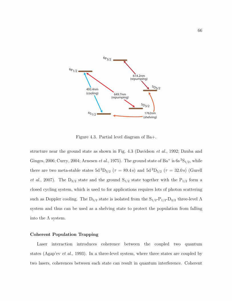
66
Figure 4.3. Partial level diagram of Ba+.
structure near the ground state as shown in Fig. 4.3 (Davidson et al., 1992; Dzuba and
Ginges, 2006; Curry, 2004; Arnesen et al., 1975). The ground state of Ba+ is 6s 2S1/2, while
there are two meta-stable states 5d 2D3/2 ( = 89.4 s) and 5d 2D5/2 ( = 32.0 s) (Gurell
et al., 2007). The D3/2 state and the ground S1/2 state together with the P1/2 form a
closed cycling system, which is used to for applications requires lots of photon scattering
such as Doppler cooling. The D5/2 state is isolated from the S1/2-P1/2-D3/2 three-level
system and thus can be used as a shelving state to protect the population from falling
into the system.
Coherent Population Trapping
Laser interaction introduces coherence between the coupled two quantum
states (Agap’ev et al., 1993). In a three-level system, where three states are coupled by
two lasers, coherences between each state can result in quantum interference. Coherent

67
population trapping (CPT) is a well-known destructive interference e↵ect in a three-level
system that, at the resonance condition, the photon scattering (absorption) in the system
is suppressed. A -type S-P-D three-level structure is found in several commonly trapped
atomic ions such as Ba+, Ca+, Sr+, and Yb+. These species are heavier atoms that have
vacant d electron orbitals. Here we briefly study this phenomenon.
The relavent system in Ba+ is labeled as |1i=6S1/2
↵, |2i=5D3/2
↵, and |3i=6P1/2
↵.
The density matrix of the system is given by
=
0
BBBB@
11 12 13
21 22 23
31 32 33
1
CCCCA(4.1)
where the ii
terms are the population in |ii and the ij
is the quantum coherence between
|ii and |ji. The dynamics of the density matrix is described by the optical Bloch equation
=i
~ [,H] +
@
@t
(4.2)
where H is the Hamiltonian, [·, ·] denotes the commutator, and @/@t is the decoher-
ence. For two lasers with Rabi frequencies 1,2 and optical frequencies !1,2 that respec-
tively couple ground states |1i and |2i to the common excitation state |3i, the system’s
Hamiltonian reads
H =
0
BBBB@
0 0 ~12 ei!1t
0 ~(!31 !32)~22 ei!2t
~12 ei!1t ~2
2 ei!2t ~!31
1
CCCCA(4.3)

68
where !31 and !32 are the energy di↵erences from |3i to, respectively, |1i and |2i. The de-coherence matrix is built in the phenomenological manner. Here we consider decoherence
only due to the spontaneous emission from |3i=P1/2
↵:
@
@t
=
0
BBBB@
133 0 12(1 + 2)13
0 233 12(1 + 2)23
12(1 + 2)31 1
2(1 + 2)32 (1 + 2)33
1
CCCCA(4.4)
with i
being the spontaneous emission rate from |3i to |ii.The optical Bloch equation Eq. (4.2) can be simplified by applying Fourier transfor-
mations. Alternatively as well as equally, the simplification can be done by factoring
into two di↵erent timescales:
ij
(t) = ij
(t)eit (4.5a)
for the corresponding term in the Hamiltonian
Hij
(t) / eit (4.5b)

69
with being the slow-varying amplitude in contrast of the high frequency exp(it) term.
With the above substitution, the optical Bloch equation Eq. (4.2) becomes
˙33 =i
21(31 13) +
i
22(32 32) (1 + 2)33 (4.6a)
˙11 = i
21(31 13) + 133 (4.6b)
˙22 = i
22(32 23) + 233 (4.6c)
˙31 = i131 +i
21(33 11) i
2221 1
2(1 + 2)31 (4.6d)
˙32 = i232 +i
22(33 22) i
2112 1
2(1 + 2)32 (4.6e)
˙21 = i(1 2)21 +i
2123 i
2231 (4.6f)
where i
= !i
!3i for i = 1, 2 is the laser detunings. Only equations for half of the
coherences terms are listed above; the other half are simply the complex conjugate of
Eqs. (4.6d) to (4.6f) since ij
= ji
.
Quantum interference in the this three-level system is established through the coher-
ence between |1i and |2i. In Eq. (4.6d), for instance, the coherence 31 is due to not only
the corresponding laser excitation i1(33 11)/2, but also the interaction between the
other laser and the ground states’ coherence i221/2. It is easy to see that, only the
real part of 21 contributes to the quantum coherence, while the imaginary part acts like
the decoherence term. Therefore, from Eq. (4.6f), a two-photon resonance condition is

70
found when 1 = 2. At this condition, the steady state population distribution is
11 = 11 =2
2
21 + 2
2
(4.7a)
22 = 22 =2
1
21 + 2
2
(4.7b)
33 = 33 = 0 (4.7c)
where there is no excitation state population even the two lasers continuously interact
with the system. The coherence 31 and 32 also vanish:
31 = 31ei!1t = 0 (4.8a)
32 = 32ei!2t = 0, (4.8b)
but there is coherence between two ground states:
21 =12
21 + 2
2
. (4.8c)
At the CPT resonance, the population is in the following quantum superposition:
2p2
1 + 22
|1i 1p2
1 + 22
|2i . (4.9)
The coherent population trapping can be easily observed with the trapped single
Ba+, as shown in Fig. 4.4. The width of the resonance primarily depends on the Rabi
frequencies of the lasers. However, the width in Fig. 4.4 is wider than expected as it is
broadened due to the laser linewidth. The Zeeman shift also contributes to the width by a

71
0
100
200
300
400
500
600
700
800
-80 -60 -40 -20 0 20 40
Cou
nts
Cooling laser detuning (MHz)
Figure 4.4. CPT resonance observed by the laser-induced spectroscopy of Ba+.
small amount. In order to avoid the CPT resonance during the laser cooling process, the
650 nm laser is actually set to blue detuned to the corresponding transition’s resonance.
A note to the decoherence terms. Other phenomenological sources of relaxation can
be added to the decoherence matrix @/@t if necessary. For instance, decoherence due
to the finite laser coherence can be written as
0
BBBB@
0 0 1130 0 123
131 232 0
1
CCCCA(4.10)

72
[check check check] where 1 and 2 are the linewidths of the laser. To describe relaxation
from |2i to |1i at rate , add the following term to @/@t:0
BBBB@
22
212 0
221 22 0
0 0 0
1
CCCCA. (4.11)
In reality, Ba+ has Zeeman sublevels in each state. The theoretical study can be
carried out in a similar manner. When the sublevels degenerate, the system is much
similar to the three-level case. When the degeneracy is lifted by, say, the magnetic field,
the system becomes an ensemble of multiple three-level CPT systems.
4.3. Laser Cooling
Cooling of a single ion’s motion is done in two stage. The Doppler cooling technique
brings the ion from room temperature to the so-called Doppler limit, which is of order
100 µK. The ion is further cooled to the ground state of the trap by means of sideband
cooling. For the projects in this thesis, Doppler laser-cooled ion is sucient. Motional
ground state cooling is required ultimately for the precision spectroscopy experiment.
Ground-state cooling of a single barium ion by two-photon Raman transition has recently
been demonstrated in Seck et al. (2016) by other members in the laboratory.
Doppler laser cooling has become a standard technique in many atomic and molecular
physics experiments, hence I will skip the introduction to this technique. We laser cool
the trapped barium ion over the 6S1/2 ! 6P1/2 transition with the 493 nm laser, while the
population is being repumped from the 5D3/2 by the 650 nm laser. As mentioned earlier,
this system could result in the coherent population trapping when the detunings of the

73
two lasers are similar. Therefore, we can not have both lasers red detuned. Only the
493 nm laser is red detuned; the 650 nm laser is set to resonant with or blue detuned to
the 5D3/2 ! 6P1/2 transition to avoid the CPT. See, e.g., Marzoli et al. (1994); Lindberg
and Javanainen (1986) for more discussions on laser cooling of a three-level system.
In passing, the issue can be avoided by doing incoherent repumping. In addition to
using an incoherent 650 nm source, the repuming can be done via the 6P3/2 excitation
state. However, since spontaneous emission from 6P3/2 to 5D5/2 is allowed, repumping on
that transition is also required. Thus, two repumping lasers are required in this scheme.
Cooling Limit
The Doppler-limited temperature is
TD
=~2k
b
(4.12)
and is achieved when the laser detuning is = /2 but independent to the laser in-
tensity (Wineland and Itano, 1979). However, when the ion is first loaded into the trap,
it can have quite a high velocity such that the Doppler shift is too large for most of the
time to have sucient photon scattering. Thus, laser cooling can be very slow initially.
We then sometimes further detune the laser to accommodate the large initial high tem-
perature. We also increased the laser intensity to have a larger scattering rate. When the
ion becomes colder, the laser is set to = /2 and I Is
with Is
being the saturation
intensity for the best Doppler cooling.
Consider the quantum motion of the trapped ion, the mean occupation number of
the motional state in the trap of secular frequency ! is given by (Wineland et al., 1987;

74
Stenholm, 1986)
n =1
exp(~!/kB
T ) 1=
1
exp(2!/) 1(4.13)
at the Doppler-limited temperature TD
. n = 7.0 when ! = 2 1MHz along the trap
axis. Additionally, the low occupation number means that the ion is suciently in the
Lamb-Dicke regime where ground state cooling can be performed by driving sideband
transitions.
4.4. Photon Counting - Time Correlation
Laser-induced fluorescence measurement allows us to detect the existence and the state
of the trapped barium ion. In this project, the fluorescence photon is collected by both a
camera and a photomultiplier tube (PMT). While the camera provides spatial resolution,
the PMT provides an excellent time domain resolution.
Fluorescence Modulation
In my single ion experiment, I searched for the time domain patterns of the fluorescence
to determine the motion of the trapped Ba+. This idea is applied to both the secular
oscillation and the RF-related micromotion. The fluorescence rate is the product of the
excitation state population Pe
and the spontaneous emission rate . For the simplicity,
we consider a stationary two-level atom whose excited population is a Lorentzian function
of the detuning . Thus, the fluorescence rate is
R() = Pe
() =
2
s
1 + s+ 42/2(4.14)

75
where s = I/Is
is the saturation parameter. As the ion oscillating with velocity amplitude
v0 and frequency !, the detuning experienced by the ion is shifted by the first order
Doppler shift:
= 0 + v0 cos!t/ (4.15)
with 0 being the laser detuning and being the wavelength of the transition. The ion’s
periodic motion hence modulates the fluorescence as R(0 + v0 cos!t/). The response
of fluorescence modulation depends on the laser detuning 0 and the amplitude v0. The
modulation is linear in the ion’s motion when the laser detuning 0 is away from the tran-
sition resonance and the corresponding Doppler is small. In this regime, the modulation
index, the coecient of the cos!t term normalized to the constant term, is
h =R0(0)
R(0)
v0
= 80/
1 + s+ 4x2/2
v0
. (4.16)
It is straightforward to find the maximum modulation
h = 2v0/p1 + s (4.17)
at 0 = ±p1 + s/2. The ± sign indicates the phase of fluorescence modulation, which
is di↵ered by when the laser is switched from red detuned to blue detuned, and vise
versa.
The second order term in the modulation is a second harmonic term as cos2 !t =
(1+cos 2!t)/2. With the definition of the modulation index in Eq. (4.17), the strength of
the second order term is R00(0)/R(0) = h2/2 regardless the sign of 0. The third order
coecient is zero. Therefore, the fluorescence rate of an oscillating ion driven around

76
0 =p1 + s/2 can be expressed as
R =s
2(1 + s)
(1 +
h2
4) + h cos!t+
h2
4cos2 !t
. (4.18)
Correlation Measurement
Experimentally, the modulation of the fluorescence is measured simply by record-
ing the fluorescence strength as a function of time. This measurement, however, is less
straightforward for the single ion experiment due to the low photon collection eciency.
Consider the typical experiment condition where the collection eciency is 104 and the
spontaneous emission rate = 9.5 107 s1 for the 6P1/2 ! 6S1/2 decay channel in the
Ba+. The photon flux is then of order 104/s, which is low compared to the trapped
ion’s oscillation frequency in the MHz range. Therefore, the arrival time (at the detector)
of each fluorescence photon is recorded instead, and the correlation of the time series is
computed to find modulations in the photon flux.
Since for either application, detecting micromotion or secular motion, the oscillation
frequency ! is known, it is convenient to measure the cross-correlation function between
the photon flux and cos!t. This measurement is approximated by measuring the his-
togram of photon counts for various phases of the oscillation. The period of the oscillation
is divided into 10 to 20 counting bins, and the histogram is fitted by Eq. (4.18) to deter-
mine the modulation index, which can be further converted to the velocity. In practice,
including only the first order term cos!t in the fitting function is sucient representative
in most applications. The correlation measurement is usually limited by the photon shot

77
noise. A good signal-to-noise ratio requires the shot noise in each counting bin being
smaller than the modulation to be observed.
Autocorrelation
When the oscillation frequency is unknown, one can compute the autocorrelation
function to find the motion. As the fluorescence photons are tagged with their arrival time,
the computation of the autocorrelation function becomes statistics on the delay times
between any two photons. Unlike the cross-correlation which measures a single frequency,
the autocorrelation method measures a large frequency range simultaneously but requires
much more data from photons. See Sheridan and Keller (2011) for an application example.
4.5. Micromotion compensation
Micromotion, introduced in Eq. (2.9), is the forced oscillation driven by the trapping
RF electric field in the Paul trap. As the micromotion amplitude is proportional to the
secular motion (the location of the ion), the micromotion vanishes only when the ion is
rest on the RF field null, which defines the trap center.
The negative impact due to the micromotion is two folds. First, the motion causes
the Doppler shift, which is a systematic error in the precision spectroscopy. Also, the
electronic noise in the RF field can disturb the ion’s secular motion through the micromo-
tion. This randomness is thus a heating source for ions in an RF trap. RF field heating
coupled by micromotion is particularly a concern for a large number of ions due to the
spatial extent. Thus, it is necessary to minimize excessive micromotion; the procedure is
called the micromotion compensation.

78
Compensation: by Imaging
A single ion is pushed away from the trap center by the DC electric field due to stray
charges and patch potentials. By biasing the trap electrodes, this field can be canceled
locally such that the ion is trapped around the field null. In the laboratory, micromotion
compensation is done in two stages. In the first stage, coarse compensation is done by
monitoring the single ion’s location on the camera while varying the strength of the RF
field. The equilibrium point of a single ion depends on the strength of the trapping field
except when it is at the field null. Therefore, if an ion is away from the trap center,
varying the RF voltage will shift its location. However, when the stray field is properly
compensated, the ion sits around the trap center and remains at the center for all RF
voltage.
For a cloud of ions as in Chapter 7, micromotion compensation can be done in a
similar manner. However, instead of monitoring the location of single ions, we adjust the
compensation DC voltages until the center of mass of the cloud remains the same when
sweeping the RF voltage.
Compensation: by Fluorescence Correlation
As mentioned in Section 4.4, the micromotion creates a modulation in the fluorescence,
which can be detected by methods of correlation functions. Therefore, micromotion can
be finely compensated by minimizing the modulation at the RF frequency in the fluo-
rescence (Berkeland et al., 1998). Figure 4.5 shows a typical fluorescence measurement
cross-correlated with the trap RF drive signal. In this measurement, each photon count-
ing bin is 5 ns wide, which divides an RF drive cycle into roughly 9 bins. The measured
modulation index is h = 0.25, and thus from Eq. (4.17), the micromotion amplitude is

79Micromotion detection
• Correlationbetween trapRFdriveandfluorescence rate.• Binwidth=5ns• h=1%↔2nmmicromotion amplitude (0.3m/speakvelocity)
Figure 4.5. Detect micromotion by autocorrelation.
v0 = 11.7m/s while the fluorescence is induced by a laser of = 493 nm and s 1;
= 9.5 107 s1. There is an addition factor ofp2 multiplied into this result as the
laser’s direction is 45 with respect to the radial direction.
Figure 4.6(a) shows micromotion modulated amplitude for various applied DC voltage
along one direction. In this measurement, excessive micromotion is minimized at 108 kV.
In Fig. 4.6(b), the compensation voltage is recorded for 21 hours to demonstrate the
drift. The trap condition can change quite frequently and hence in the future experiment,
excessive micromotion needs to be checked constantly.
Other Methods
Compensation based on the ion’s location or the fluorescence modulation are the two
common approaches. Yet, Ibaraki et al. (2011) demonstrated micromotion compensation
by means of parametric resonance. In this scheme, the parametric excitation is done
by amplitude modulating the trapping RF voltage. When modulating at the secular

80ModulationversusappliedvoltageModulation indexhchangesby0.025pervolt.
(a)
Compensationdrift…
Thebariumovenwasonfor900satt=0.(b)
Figure 4.6. Micromotion amplitude as a function of bias DC
frequency, the ion’s oscillation is resonantly excited unless it is at the RF null. Therefore,
the parametric resonance can be used to detect excessive micromotion.
Finally, if the ion is in the Lamb-Dicke regime, sideband transitions due to the micro-
motion would be resolved. Hence, compensation is done by minimizing the corresponding
sideband amplitude.
4.6. Secular Oscillation
This section talks about the characterization of the ion’s secular motion, which pro-
vides preliminary information for the experiment presented in the next chapter as well as
other applications. We especially focus on the measurement of the secular frequency in
the axial (z) direction.
The secular frequency is probed by finding the resonance between the ion’s motion and
its external driving force. The simplest motional excitation is an AC electric field along
the axial direction, which is provided by driving one of the endcap electrodes with an AC
signal. The single ion is continuously laser cooled. When the ion’s motion in the trap

81
(a) (b)
Figure 4.7. Tickling on end cap
resonants with the AC electric field, the oscillation amplitude quickly builds up such that
the Doppler shift becomes too large for sucient laser scattering. Thus the fluorescence
rate drops at the resonance. Figure 4.7(a) shows a typical spectrum of the axial secular
motion. The dropping of fluorescence at 203 200 kHz is identified as the axial secular
mode. To further justify, the square of the resonance frequency for various endcap DC
voltage Vec is measured in Fig. 4.7(b) and a linear relationship is observed. The slope is
6774.9 kHz2/V and is equal to z
e/(2)2mz20 according to Eq. (2.8) with the correction of
the geometric factor z
. Therefore, the geometric factor is measured to be z
= 0.41 with
z0 = 0.95mm for this ion trap. The finite element analysis of this trap yields z
= 0.54.
The discrepancy is most likely due to the dimensional error in the trap.
The trapped ion represents a high-quality mechanical oscillator and therefore presents
a narrow linewidth in its motional spectrum. Although the ion is laser cooled during the
measurement, damping due to the Doppler cooling is, in fact, negligible. Another source
of damping is the resistance seen by the imaging charge. Finally, the spectral width is

82
Figure 4.8. Autocorrelation function of the oscillating ion.
most likely due to the uncertainty of the secular frequency originated from the endcap
voltage fluctuation.
The motional excitation can be provided by the light pressure as well. In this method,
the cooling laser (493 nm) is amplitude modulated at a certain frequency to provide a
periodic optical force. The shape of the modulation is less critical here; I simply apply
the square wave modulation. The fluorescence of the ion integrated over multiple periods
drops, as in the previous setup when the optical force resonantly excites the secular
motion.
The secular motion can be probed by the photon correlation function introduced in
Section 4.4 as well. To demonstrate, the ion is driven by a weak AC electric field as in the
earlier experiment. The detected fluorescence photons are tagged with their arrival time
and the autocorrelation function is computed. A typical result is shown in Fig. 4.8. There
is an obvious oscillation with a period 3.3 µs coming from the secular motion. Furthermore,
the amplitude of the oscillation has a decay time around 63 µs. In Table 4.1, the frequency
response obtained by means of photon correlation is shown.

83
Table 4.1. Frequency response
Drive frequency(kHz) Measured period(µs) Measure frequency(kHz) Modulation index
300.3 3.329(6) 300.390 0.023(4)300.4 3.332(3) 300.120 0.040(4)300.5 3.328(2) 300.480 0.084(4)300.6 3.326(2) 300.661 0.059(4)300.7 3.325(11) 300.751 0.012(4)
In the next chapter, we will convert the secular frequency measurement into an internal
state readout protocol for the single ion spectroscopy experiment.

84
CHAPTER 5
Coherent Motion Single Ion State Readout
This chapter presens the development of state readout by coherent motion, which was
published in Lin et al. (2013).
5.1. Motivation
The high quality of environmental isolation, storage time, and particle localization
provided by ion traps creates an excellent environment for quantum control and preci-
sion spectroscopy (Leibfried et al., 2003). To date, nearly all few-ion experiments have
accomplished control and addressing by relying on laser-accessible closed-cycle optical
transitions, which occur in only a small number of atomic ion species. An essential fea-
ture required for extending the power of ion traps to other atomic and molecular species
is the ability to perform non-destructive internal state readout with a small or vanishing
numbers of scattered photons (Schmidt et al., 2006; Leibfried, 2012; Ding and Matsuke-
vich, 2012; Mur-Petit et al., 2012; Clark et al., 2010). Ability to control and monitor
new atomic and molecular ion species could open new possibilities in such areas as quan-
tum information processing, parity-violation studies, search for time-reversal symmetry
breaking, and search for time-variation of fundamental constants.
Here, we study the excitation of a Doppler-cooled single barium (Ba+) ion in a har-
monic trapping potential with negligible damping, under the influence of a resonantly
pulsed radiation pressure force in the regime of few photon scattering. A pulsed radiation

85
pressure force, in the regime of large scattering numbers, has previously been used for
few-ion mass spectrometry (Drewsen et al., 2004). In modeling and experiment, we find
that phase-locking behavior allows ecient energy transfer to the ion oscillator, such that
scattering of order one hundred photons e↵ectively separates the driven velocity from
the Doppler-cooled distribution. Since motional excitation by photon scattering is con-
ditional upon the ion’s internal state, a pulsed radiation pressure force could be used to
transfer internal state information from a molecular or atomic spectroscopy ion with only
a marginally closed-cycle transition onto a co-trapped logic ion used for state readout.
State readout of a non-cycling spectroscopy ion has been accomplished by first reducing its
temperature by laser-cooling a co-trapped logic ion, then using sophisticated protocols to
map its internal state information onto detectable motion of the two-ion crystal (Schmidt
et al., 2005; Hume et al., 2011). A pulsed radiation pressure force applied to a molecular
or atomic spectroscopy ion with only a marginally closed-cycle transition could o↵er a
new and simple means to accomplish the state mapping.
5.2. Pulse-Driven Oscillator
We treat the ion as an undamped oscillator because damping from radiation and
resistive losses are negligible, and damping due to o↵-resonant photon scattering is also
unimportant, as the ion motion is small in our experiment.
The equation of motion of a harmonic oscillator driven resonantly by a square pulse
train is:
x00(t) + !2x(t) = F (t)/m. (5.1)

86
In the above equation, x(t) is the position of the oscillator at time t; omega is the secular
frequency of the oscillator; m is the mass. The driving force is a periodic function with
period T = 2/! and for 0 < t < T it can be written as
F (x) =
8>><
>>:
, 0 t < DT
0, DT t < T
(5.2)
with being the drive strength and D the duty cycle. Because the driven oscillator phase
locks such that photon scattering transfers maximum energy (with ion velocity along
the laser direction at the time of scattering,) excitation by a pulse train with small duty
cycle D is more ecient per photon than excitation by a sinusoidally modulated radiation
pressure force. For the moment neglecting stochastic aspects of photon scattering, the
driving force is given by = ~ke
/p2, where k is the photon wave number,
e
is the
excited state population, and is the scattering rate. Thep2 factor accounts for the 45
angle between the force and the motion in our experiment; 1020 N for typical visible
dipole transitions, with e
= 0.3 determined experimentally.
To study Eq. (5.1) I first find the Green’s function G(t, t0) of this system:
G(t t0) =1
!(t t0) sin(!(t t0)) (5.3)
where (t t0) is the step function. The Green’s function describes the response due to
an infinitesimal kicking to the oscillator and is the solution to the following equation:
G00(t) + !2G(t) = (t t0). (5.4)

87
By the Green’s Theorem, the full solution to Eq. (5.1) can be expressed as
x(t) = A sin(!t+ ) +1
m
Zt
1G(t t0)F (t)dt0. (5.5)
Let’s first consider the response due to only one pulse. By pluggin Eq. (5.2) into Eq. (5.5)
and carrying out the integration from t = 0 to DT , we obtain
x(t) = A sin(!t+ ) +2
m!2sin
!DT
2
sin
!t !DT
2
.
Further let !DT = 2D and the above expression therefore becomes
x(t) =
A cos+
m!2sin
sin!t+
A sin+
m!2(cos 1)
cos!t . (5.6)
Namely, after the application of a single pulse,
x0(t) = A sin(!t+ )! x1(t) = A1 sin(!t+ 1) (5.7)
for
A1 =q
c21 + c22 (5.8a)
and
tan1 = c2/c1 (5.8b)
with
c1 = A cos+
m!2sin (5.8c)
c2 = A sin+
m!2(cos 1) (5.8d)

88
Hence, a recursive equation can be set up to account for each consecutive pulse from the
pulse train. That is, a equation to describe the evolution
(A0,0)! (A1,1)! · · ·! (An
,n
) (5.9)
after the application of n pulses.
Phase Evolution
We are interested in the phase shift due to the pulse drive. Equation (5.8b) is explicitly
tan1 =A sin+
m!
2 (cos 1)
A cos+
m!
2 sin.
Now, write 1 = + and recall the following identity:
tan1 = tan(+ ) =tan+ tan
1 tan tan (5.10)
=sin+ cos tan
cos sin tan .
By comparing the above two expression, we can find that
tan =2 sin/2 sin(+/2)
Am!2/+ 2 sin/2 cos(+/2). (5.11)
Note that the oscillator’s phase eventually is locked to the drive at c
= /2.
Therefore, to study the phase-locking mechanism, we write = c
+ = /2 + .
When 1, the above equation hence become
tan = 2 sin/2
Am!2/+ 2 sin/2 (5.12)

89
which describes a negative feedback between and . By realizing = n
n1 at the
application of the n-th pulse, Eq. (5.12) is therefore the recursion equation for n
and
the solution is
n
=
1 2 sin/2
Am!2/+ 2 sin/2
n
0 (5.13)
=
Am!2/
Am!2/+ 2 sin/2
n
0.
The phase is locked to its final value exponentially in time with a time constant
= T/ ln
1 +
2 sin/2
Am!2
. (5.14)
It is to see that a rapid phase-locking is provided by a strong drive, Am!2, and
50% duty cycle such that sin/2 = sin D = 1.
Amplitude Evolution
Let’s first find the condition for maximum amplitude growth. From Eq. (5.8a),
A21 = c21 + c22 (5.15)
= (A+2 sin/2
m!2)2 4A
m!2sin
2
1 cos(+
2)
.
The increment is maximized when the phase equals to
c
2
= D (5.16)
and the growth is
A1 A =2 sin D
m!2. (5.17)

90
In general, Eq. (5.15) can be approximated as
A21 = A2 + 2A cos (5.18)
where = 2 sin(D)/m!2 being much smaller than A in this experiment. In our experi-
ment = 2.7 nm and A0 34 nm for a Ba+ ion at the Doppler limit. With A1 = A+A,
we further obtain
A cos, (5.19a)
which is the recursion equation of the amplitude. Similarly,
=A
sin (5.19b)
is the recursion equation of the phase.
By treating Eq. (5.19) as continuous in n and integrating, we find closed-form expres-
sions:
An
=p
(A0 sin0)2 + (n+ A0 cos0)2 (5.20a)
n
= cos1(n+ A0 cos0
An
). (5.20b)
The peak velocity of the oscillator after n cycles is then Vn
= !An
and can be experimen-
tally measured by the Doppler velocimetry introduced in Section 4.4 with extreme high
sensitivity (Berkeland et al., 1998; Biercuk et al., 2010).
We compare 5.20 to a molecular dynamics simulation which takes the random timing
and spontaneous emission angle of photon scattering into account. For the sample ini-
tial conditions and simulated scattering history shown in Fig. 5.1, the simulation di↵ers
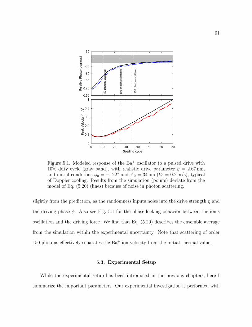
91
!"#$%&'"l()$*"ls+",-""*(
)035
)025
)c5
)p5
)95
5
95
35l.)/%/0*l*1$%%"-"+
055l.)/%/0*l*1$%%"-"+
035l.)/%/0*l*1$%%"-"+
("$2l3"#/1&%4ls51*(
5
5-2
5-6
5-p
5-n
0
6""+&0,l141#"
5 05 25 95 65 35 p5 o5
Figure 5.1. Modeled response of the Ba+ oscillator to a pulsed drive with10% duty cycle (gray band), with realistic drive parameter = 2.67 nm,and initial conditions 0 = 122 and A0 = 34 nm (V0 = 0.2m/s), typicalof Doppler cooling. Results from the simulation (points) deviate from themodel of Eq. (5.20) (lines) because of noise in photon scattering.
slightly from the prediction, as the randomness inputs noise into the drive strength and
the driving phase . Also see Fig. 5.1 for the phase-locking behavior between the ion’s
oscillation and the driving force. We find that Eq. (5.20) describes the ensemble average
from the simulation within the experimental uncertainty. Note that scattering of order
150 photons e↵ectively separates the Ba+ ion velocity from the initial thermal value.
5.3. Experimental Setup
While the experimental setup has been introduced in the previous chapters, here I
summarize the important parameters. Our experimental investigation is performed with

92
Figure 5.2. Experimental timing sequence.
a single 138Ba+ along trap’s axial mode with a secular frequency !z
= 2 926 kHz. The
manipulation of the ion is done by driving the blue 6S1/2 ! 6P1/2 transition (493.4 nm,
S
= 215.2MHz) and the red 5D3/2 ! 6P1/2 transition (649.7 nm, D
= 24.9MHz).
The two lasers are focused on the ion and co-propagate at 45 with respect to the trap z-
axis. For Doppler cooling, we set the blue laser intensity to 2 Isat
with 15MHz detuning;
the red repumping laser intensity is 10 Isat
, detuned by 20MHz.
In order to detect few-photon seeded motion of the trapped ion, we use a motional
amplification scheme, where a continuous-wave (CW) laser is blue-detuned from a cycling
transition. See Section 5.4. Fluorescence from the ion is detected by a photomultiplier
tube (PMT) with an overall eciency of 0.1% including a bandpass filter transmitting
only the blue light. We use an FPGA-based counter to perform photon statistics.
The major cycle of the experiment consists of seeding the motion, amplification, and
resetting by Doppler cooling, as depicted in Fig. 5.2. To seed the ion motion, we chop
the blue laser at the secular frequency !z
; the laser intensity is set to 10 Isat
with zero
detuning; the seeding pulse train is applied for time ts
. The blue laser detuning is then
set to 15MHz for time ta
to amplify the seeded oscillation; ta
= 10ms was chosen by
experimental optimization. After amplification, the laser detuning is then set back to

93
15MHz to damp the excited ion. The repumping laser is not altered for each stage of
the experiment. To detect the motion, we collect fluorescence from the last 4ms of the
amplification stage and the first 4 ms of the cooling stage. The above experiment cycle is
repeated every 50ms, and we integrate for 2 seconds to obtain the modulated fluorescence
signal. These 40 cycles typically yield 1000 photon counts, collected by the FPGA into
20 timing bins of width 46.7 ns. Ion motion is detected as a modulation in photon arrival
times with modulation amplitude h determined by fitting the correlation function g() to
1 + h cos(!z
( 0)) where is the time referenced to each secular motion cycle, and 0
compensates for constant experimental phase delays.
5.4. Coherent Motion Amplification
The seeded ion has a very small oscillation amplitude. For its motion to be detected by
the fluorescence technique, the oscillation needs to be coherently amplified. We amplified
the ion’s secular motion in the trap by laser scattering, based on the technique in Kaplan
(2009); Vahala et al. (2009). This technique has been used to detect motion induced by
electrostatic (Knunz et al., 2010), radiation pressure (Sheridan et al., 2012), and optical
dipole forces (Hume et al., 2011).
While the scattering of a red-detuned laser removes the momentum from the ion,
a blue-detuned laser does the opposite. However, the blue-detuned laser does not add
momentum to the ion randomly. As the ion has a secular oscillation, the scattering rate is
modulated and thus the corresponding radiation pressure is modulated as well. Therefore,
the ion, in fact, sees a periodic driving force due to the laser scattering. Since the periodic
drive is in phase with the oscillation, it amplifies the motion coherently. The mechanism
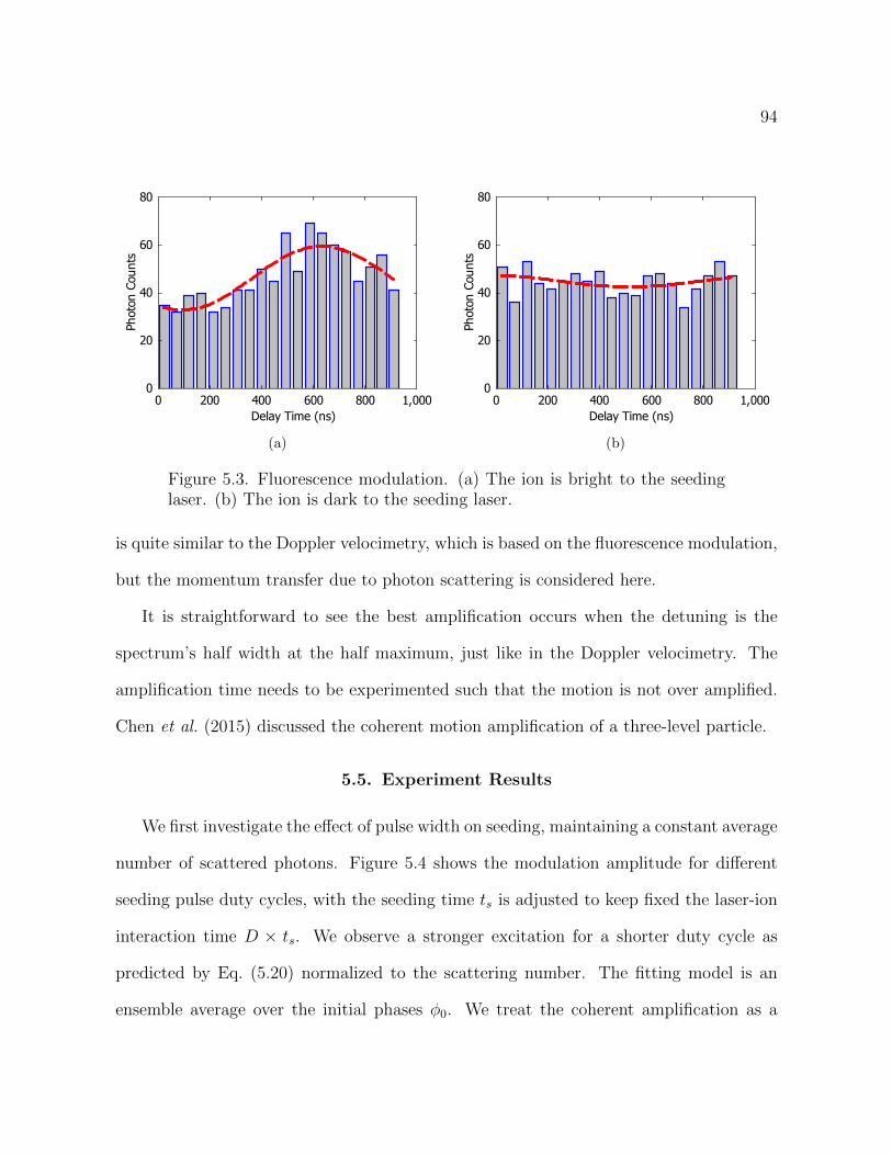
94Photo
n C
ounts
0
20
40
60
80
Delay Time (ns)
0 200 400 600 800 1,000
(a)
Photo
n C
ounts
0
20
40
60
80
Delay Time (ns)
0 200 400 600 800 1,000
(b)
Figure 5.3. Fluorescence modulation. (a) The ion is bright to the seedinglaser. (b) The ion is dark to the seeding laser.
is quite similar to the Doppler velocimetry, which is based on the fluorescence modulation,
but the momentum transfer due to photon scattering is considered here.
It is straightforward to see the best amplification occurs when the detuning is the
spectrum’s half width at the half maximum, just like in the Doppler velocimetry. The
amplification time needs to be experimented such that the motion is not over amplified.
Chen et al. (2015) discussed the coherent motion amplification of a three-level particle.
5.5. Experiment Results
We first investigate the e↵ect of pulse width on seeding, maintaining a constant average
number of scattered photons. Figure 5.4 shows the modulation amplitude for di↵erent
seeding pulse duty cycles, with the seeding time ts
is adjusted to keep fixed the laser-ion
interaction time D ts
. We observe a stronger excitation for a shorter duty cycle as
predicted by Eq. (5.20) normalized to the scattering number. The fitting model is an
ensemble average over the initial phases 0. We treat the coherent amplification as a

95
!"#$%&'(")d*+,%('$#-d.
2
2.3
2.D
2.y
/$'0d102%-d/
2 2.3 2.D 2.y 2.C 2.c
Figure 5.4. Measured modulation amplitude mean (points) and standarddeviation (bars) versus seeding duty cycle, with seeding time varied to main-tain D t
s
= 4 µs; data were collected over 30 trials. Averaging Eq. (5.20)over initial phases and fitting for amplification-stage gain yields the solidcurve.
constant velocity gain ga
(here ga
= 2), found from a single-parameter fit to the data,
and then convert the amplified ion velocity into modulation amplitude according to a
Lorentzian spectrum using an experimentally determined full-width-half-maximum of 30
MHz. The deviation between the experiment and the theory is attributed to the known
variation of the amplification gain as the laser frequencies drift during the experiment.
Figure 5.5 shows the measured modulation amplitude versus seeding time, using
D = 0.1, with the predicted response from Eq. (5.20) and a single-parameter fit for
amplification gain (here ga
= 2.7.) Due to the initial distribution of oscillator phases,
the model predicts slow ensemble-averaged velocity buildup at short times, until some
degree of phase locking has occurred (see also Fig. 5.1.) The time scale for phase-locking

96
!"#$%&'(")d*+,%('$#-d.
2
2.3
2.4
2.5
2.6
2.S
2.g
/--#()0d1(+-d'2dA32m
2 42 62 g2 s2 322 342
Figure 5.5. Modulation amplitude versus seeding time, when the seedingpulses excite an S-state ion (red), and when the ion is shelved in the D-state (blue). Each point is the average of 30 measurements, with the verticalbars showing the distribution standard deviation (rather than the error onthe mean). The predicted response (black curve) is from Eq. (5.20), fittingfor amplification-stage gain.
is given by A0/ 13 cycles, or 14µs in this work. Once the phase is locked, all the pho-
ton momentum contributes to secular motion excitation coherently. Since the oscillation
converts to fluorescence modulation approximately linearly, modulation amplitude goes
linearly with the seeding time for a phase-locked oscillator.
5.6. Spectroscopy Application
We now consider the application of our pulsed seeding technique to internal state read-
out by mapping the internal state onto ion motion. Figure 5.5 also shows the response
from an unseeded ion, obtained by optically pumping into the D3/2 state before seeding
pulses are applied; before amplification, the ion is repumped to the S1/2 state. In the

97
!"#$%&
A
m
p
e
h
.
'"(#)*%+"$u,-.)+%#(/u0
a h aA aAh am amh ap aph ae
u&//(/(u1"2ue 3&u$"$&//(/(
Figure 5.6. Distribution of the modulation amplitudes, measured after seed-ing the motion for 40 µs (red histogram) and for an unseeded ion (blue his-togram). The simulation (solid curves) accounts for noise in ion dynamicsand shot noise in detection. Amplification gain is the single fit parameter.
context of a spectroscopy experiment, (failed) seeding from the D3/2 state simulates state
readout after a successfully driven spectroscopy transition, while (successful) seeding from
the S1/2 state simulates state readout after a failed spectroscopy transition (or vice versa.)
Based on the magnitude of the dark state baseline, seeding for ts
40 µs is sucient to
create Ba+ motion well separated from the noise floor after amplification and our integra-
tion over 40 excitation/detection cycles. For this seeding time, there are approximately
n
= 150 photons scattered per excitation cycle, and the measured fluorescence modu-
lation is h = 0.24. In Fig. 5.6 we show the experimental h distributions for seeded and
unseeded ions, again using D = 0.1, along with the simulated results (with ga
= 2.5 the
only fit parameter) accounting for various noise sources summarized in Table 5.1.

98
Figure 5.7. Determination of modulation index from data with 30 averagecounts per bin.
5.7. Error Sources and Improvement
In our experimental implementation, the major source of noise is low photon detection
eciency. Photon shot noise propagates through the data analysis and contributes to the
width. For example, Fig. 5.7 shows the determination of the modulation index based on
data that has on average 30 counts per bin. One can see that, with such low photon
counts, h = 0.1 is roughly the detection limit.
In addition to the seeding noise already discussed, the coherent amplification processes
injects noise into the ion motion, as the photon scattering has random spatial and tempo-
ral components. In Table 5.1 we model this noise term as a random walk in velocity space,
(v)2 v2r
e
ta
, where vr
= ~k/m is the recoil velocity and e
0.02 during amplifica-
tion. Overall, the summarized error sources characterize our state-detection uncertainty
and form the distribution in Fig. 5.6. If we discriminate whether the ion’s motion is
excited by a threshold value hth
= 0.12, where the two distributions intersect, the false
positive rate is estimated to be 3.2% and the false negative rate is 3.8%.

99
Table 5.1. Modeled contribution of various noise sources to the distributionwidth of the modulation amplitude, for n
= 150 yielding h = 0.20. Data isintegrated over N excitation/detection cycles, with initial ion temperature360 µK, t
s
= 40 µs, ta
= 10ms, and ga
= 2.5. For N = 1, consider only thenoise intrinsic to ideal single-shot excitation, say, for perfect fluorescencecollection or for sustained oscillation during detection. For N = 40, thereare 1000 fluorescence photon counts spread over 20 timing bins. The lastline represents the quadrature addition of all sources.
Source h, N = 1 h, N = 40
Photon counting 0 0.043Initial thermal motion 0.072 0.011Seeding stage 0.032 0.005Amplification stage 0.114 0.018Total width 0.139 0.048
Note that the measurement uncertainty is reduced by N1/2 after integrating over N
excitation/detection cycles. (N = 40 in this work.) However, the required number of
photons for state discrimination is then N n
, where n
150 is the seeding photon
number required here. Currently, we perform detection while the ion velocity is either
being amplified or cooled. An important improvement, which would eliminate the need to
integrate over N > 1 excitation cycles, would be to simultaneously damp and amplify the
oscillation with both the cooling and the repumping laser to achieve self-limiting sustained
large-amplitude oscillation (Vahala et al., 2009; Knunz et al., 2010). The number of
scattered photons required for seeding the motion could also be reduced by a factor ofp2
by sending the laser along the trap axis, making the photon momentum parallel to the
secular motion direction. The detection sensitivity could also be enhanced by measuring
the modulation amplitude with lock-in technique and increasing the photon detection
eciency (Streed et al., 2011; Shu et al., 2010). Seeding a lighter ion would require fewer
scattered photons, as the ratio of recoil to thermal velocity goes as m1/2.
100
5.8. Outloook
If the trap is loaded with both a spectroscopy ion (used for the seeding stage) and
a fluorescing logic ion (used first to Doppler cool the two-ion system then later in the
amplification/detection stage), this state discrimination method can be applied to spec-
troscopy experiments. Further study of seeding behavior in a 2-ion crystal is required,
but we expect approximately a degradation factor of 2 from the 1-ion seeding eciency,
to account for excitation of additional non-detected normal modes.
It is instructive to compare this state readout approach to other protocols using a co-
trapped spectroscopy and logic ion. Quantum logic spectroscopy (Schmidt et al., 2005)
does not use spectroscopy ion scattering, but places restrictions on transition linewidth
and wavelength, also requiring ground state cooling and logic ion shelving. Coherent
excitation by an optical dipole force (Hume et al., 2011) also does not scatter from the
spectroscopy ion and relaxes ground-state cooling and shelving constraints, but it requires
a suitable transition and challenging alignment of counter-propagating beams onto a dark
ion. Our pulsed-excitation method does not require ground state cooling or shelving,
can in principle be applied to any transition, and is quite simple to implement; how-
ever, it is limited to spectroscopy species with partially closed-cycle transitions allowing
repeated scattering. Finally, sympathetic heating spectroscopy (Clark et al., 2010) uses
non-modulated spectroscopy ion scattering, requiring much more scattered photons than
the phase-coherent approach described here.
To conclude, we have modeled and experimentally studied the state-dependent exci-
tation of a single-ion oscillator impulsively driven at the trap frequency. Rapid phase-
locking behavior results in ecient energy transfer; scattering approximately n
= 150

101
photons e↵ectively separates the bright and dark state velocity distributions. However,
our detection method is currently inecient, requiring N = 40 excitation/detection cy-
cles to build up photon statistics, such that 6000 scattered photons are currently needed
to determine the internal state. Implementation of sustained amplification with phase-
sensitive detection, along with other technical improvements discussed above, could reduce
scattering to the small number (order 100 and N = 1) required to make a seeded exci-
tation detectable above the thermal and scattering noise. With a co-trapped fluorescing
ion used for the amplification and detection, this motional seeding technique could be
useful in spectroscopy experiments on molecular ions with semi-closed transitions (Lien
et al., 2011; Nguyen and Odom, 2011; Nguyen et al., 2011), atomic ions with slow cycling
transitions, and in bichromatic force schemes where cycling is enhanced by stimulated
emission (Voitsekhovich et al., 1989; Grimm et al., 1990; Chieda and Eyler, 2011). This
resonant impulsive excitation technique could also be used to coherently excite selected
normal modes of larger trapped ion crystals.

102
CHAPTER 6
Apparatus for the Molecular Ion Trap
This chapter introduces the apparatus for studying the internal state cooling of molec-
ular ions, specifically the silicon monoxide cation or SiO+. Part of the apparatus used in
this project is common to those in the single ion project. The main di↵erence is the trap
itself, the laser systems, and the detecting method.
In this molecular cooling project, an ion cloud is trapped in a centimeter-scale linear
Paul trap. A larger number of ions provides larger signal and thus makes data collection
faster when researching molecules. The lasers used to manipulate the molecular ion
are usually in the UV wavelengths; some of the lasers are high power pulsed lasers.
Detecting trapped molecular ions with fluorescence is harder because of the lack of cycling
transitions. Hence, we turned to the mass spectroscopy.
6.1. The Molecular Ion Trap
Geometry
This larger scale ion trap is also a linear Paul trap. Refer to Fig. 6.1 for the trap’s
outline. The trap has four stainless steel rods as the electrodes for the RF field. These
electrodes can be biased each with a di↵erent voltage for the micromotion compensation
or other applications. The endcaps are tube electrodes such there the axial clearance
for lasers. These electrodes are mounted on two macro pieces, and the trap assembly is
mounted on a vacuum blank flange attached to the chamber.

103
14.64.54
Φ6.86
Φ4.16/2.54
Endcap plate+tube Trap cross-section
Figure 6.1. Molecular ion trap outline
This trap has r0 = 3mm and z0 = 7.3mm; the geometric factors are r
= 0.25 and
z
= 0.42 obtained from the trap potential simulation (Appendix B.2).
RF Source
The molecular ion trap is driven at a lower AC frequency such that with tangible
voltage. For this trap geometry, a few hundred volts at 2 to 4MHz is able to provide
simultaneously trapping of species we are interested in, such as Si+, SiO+, and Ba+.
Either the coaxial or the helical resonator is not suitable for this application since the
physical size of the resonator is unrealistically large for 2 to 4MHz. Instead, we build an
inductor-capacitor (LC) resonance circuit to generate the high voltage for the trap.
The LC circuit is shown in Fig. 6.2(a). Like the other trap, the capacitance in the
circuit is mainly from the trap itself and contact connections such as at the vacuum
electrical feedthroughs; in practice, we expect of order 100 pF capacitance. For a resonance

104
DC input
RF input
RF output
1k 1k
6.8 pF 6.8 pF
100 nF
(a) Schematic.
(b) The inductor.
Figure 6.2. RF source with toroidal inductor.
at 2 to 4MHz, the required inductance is 15 to 60 µH and is realized often by a ferrite
toroid coil.
Ferrite is a ferromagnetic ceramic material that has a large relative magnetic per-
meability µr
= µ/µ0 = 103 at frequencies from DC to a few MHz. Beyond this range,
the ferromagnetic response quickly rolls o↵ as the phase between the magnetic field and
the magnetization becoming larger. The out-of-phase ferromagnetic response not only
reduces the permeability but also become resistive, so it is important to choose a ferrite
core that can operate at the desired drive frequency. Two interesting references regarding
ferrite materials are Goldfarb and Bussey (1987); Ott et al. (2003).

105
The specification of the toroid inductor can be estimated based on
L =µN2A
l(6.1)
where L is the inductance, µ is the permeability of the core, N is the number of turns in
the coil, A is the area of the coil cross-section, and l is the length of the coil. However,
as other parameters such as the capacitance is known less accurately, the dimension of
the inductor (usually the coil’s number of turns) is oftentimes adjusted until the desired
resonant frequency is obtained. Figure 6.2(b) shows the ferrite toroid inductor used in
this molecular ion trap RF electronics.
The driving signal is capacitively coupled into the circuit through the 100 nF capacitor
in Fig. 6.2(a). This configuration allows us to add a DC voltage to the electrode for
creating a DC electric field in the radial direction. Two of the RF electrodes (from one
diagonal pair) are each connected to one circuit; the two inductors from each copy of the
circuits, however, share the same ferrite core and are built as matched as possible so the
RF voltages on both electrodes can be the same.
The response of the LC resonant circuit is probed simply by measuring the voltage
at the inductor’s output end, which is connected to the trap electrode directly. With a
few watts of pump power, several hundred volts can be generated at the electrodes. It is,
however, not possible to generate higher voltages in this circuit with more pump power
as the response saturates. This is due to the magnetic saturation of the ferrite core. Also,
the RF amplifier is no longer linear at high output.

106
As in the single ion trap electronics, there is a low-pass filter each between the DC
voltage supply and the electrode. The RC low-pass filter uses R = 1k and C = 6.8 nF,
which has a 3 dB frequency of 23.4 kHz.
6.2. Lasers
The lasers for cooling barium ions were described in Section 3.4. This section will
cover other laser systems for manipulating SiO+.
Continuum Mini-Lite
This is a low power pulsed Nd:YAG laser that outputs 10 ns pulses at 10Hz repetition
rate. The 1064 nm and the second harmonic 532 nm outputs are used in the laser ablation
process for atomic or molecular source generation. The fourth harmonic 266 nm UV
output is an easy solution to get energetic photons in the ionization or dissociation process.
Spectra-Physics Quanta-Ray YAG
This is high power (>750mJ per pulse at 532 nm) is the pump source for the pulsed
dye lasers or the optical parametric oscillator (OPO) lasers.
Spectra Physics Sirah Dye Laser; Lambda Physik Dye Laser
These lasers provide light sources for resonantly driving transitions in the SiO and
SiO+. The selective transitions are used in the source production and the analyzing
the molecular internal states. The dye laser uses a color dye as the laser gain medium.
Although each dye has a specific operating wavelength length, the visible and near IR
spectrum have been mostly covered by all sorts of laser dyes. The dye laser pulses can be
further frequency doubled to generate the UV wavelength.

107
In general, the dye lasers’ wavelengths are measured by a spectrometer, which has
a resolution of a few wavenumber at best. The Spectra-Physics Sirah dye laser has a
narrower linewidth and thus can be measured by a wavelength meter instead.
Spectra-Physics Mai-Tai
The is a turn-key mode-locked Ti:Sapphire femtosecond laser for cooling of the silicon
monoxide ions. The cooling mechanism will be discussed in Section 8.3. The preparation
of the laser for this application will be detailed in Chapter 9.
6.3. Fluorescence Detection
The geometry of the imaging system for the molecular ion trap is similar to the one
used in the single ion experiment. Limited by the obstruction of the trap electrodes,
the emission from a single ion at the trap center has a solid angle of 0.151 sr, equivalent
to 1.2% of the total fluorescence. The photon is first collected by an f = 100mm lens
followed by a relay telescope consisting an f = 200mm and an f = 50mm lenses. The
light is then split by a dichromatic mirror such that photons of di↵erent colors are imaged
at two cameras at the same time. Specifically, the dichromatic mirror separates the UV
photons from the visible ones. In each branch, there is an f = 125mm lens to focus the
beam onto the camera. The outline is also depicted in Fig. 6.3 as well. All the lenses in
this imaging system are achromatic doublet lenses. The overall magnification is 5X.
Alignment
While the imaging system is constructed in the infinity corrected configuration, com-
ponents can be separated into groups for alignment. A laser with the wavelength of
interest is used as a calibration source during the alignment; we used the 385 nm laser

108
Andor EMCCD looks at 493 nm
fluorescence
Andor iCCD looks at 385 nm
fluorescence
(1)
(2)(3) (4) (5)
(6)
(7)
(8)
(1) Single ions emit 385 nm or 493 nm fluorescence. N.A. 0.22. (2) Vacuum viewport. Fused silica, about 10 mm thick. (3) f = 100 mm, achromatic doublet (4) f = 200 mm, achromatic doublet (5) f = 50 mm, achromatic doublet (6) dichroic mirror transmits 493 nm and reflects 385 nm (7)(8) f = 125 mm, achromatic doublet
Figure 6.3. Imaging system for the molecular ion trap. (1) Single ion source,N.A. = 0.22. (2) Vacuum viewport; fused silica, about 10mm thick. (3)f=100mm achromatic doublet. (4) f=200mm achromatic doublet. (5)f=50mm achromatic doublet. (6) Dichroic mirror transmits 493 nm andreflects 385 nm. (7)(8) f=125mm achromatic doublet.
as the system is built to observe fluorescence from SiO+ in the future. The calibration
laser source is output coupled from a single fiber to ensure a good Gaussian mode. The
collimation is checked by a shear interferometer.
The tube lens (L4 in Fig. 6.3) is aligned to the camera by making the laser best focused
on the sensors. The relay telescope, which has two lenses (L2 and L3) confocal, takes a
collimated input and makes a collimated output beam as well. Once these two modules
are aligned, they are assembled together with other optics such as the dichroic mirror and
other filters. The distance between modules is less critical due to the infinity corrected
configuration. The objective lens (L1) is the last piece to be installed and is adjusted
until a clear image is formed.

109
Aberration
The aberration of the imaging system is analyzed here by the optical ray tracing
technique. In Fig. 6.4, the transverse ray aberration (TRA) of the imaging system used
in this molecular ion project is plotted. The TRA plot shows the correspondence between
the ray’s initial location at the objective lens (horizontal axis) and its final location on
the imaging plane (vertical axis). In this simulation, the rays are originated from a point
source representing the ion. Therefore, a flat TRA curve would indicate a sharp image of
the point source. However, the curve in Fig. 6.4 is flat only in a smaller region closed to the
center of the optics. At larger aperture location, rays severely deviate from the focal spot.
That is, not all of the collected fluorescence contributes to the image constructively; some
of the light is actually scattered away and creates the halo around the image. Figure 6.5
shows some sample images of ions with aberrations.
The major type of the aberration the imaging system su↵ering from is spherical. While
the transverse spherical aberration grows as the cube of the aperture, it significantly lowers
the imaging ecient. In Fig. 6.6, the collection eciency for various sizes of the region of
interest is measured. In this experiment, the ion is made to fluoresce a fixed amount of
photons. Controlled fluorescence is achieved by first pumping the barium into the 5D3/2
state. Then, the camera is armed to detect signal while the 650 nm laser pumps the
population into the 6S1/2. When the spontaneous decay to 6S1/2 happens, there is exactly
one photon at 493 nm emitted. Therefore, the number of 493 nm fluorescence photons
generated is equal to the times this sequence is repeated for. This experiment provides
an accurate way to measure the fluorescence detection eciency.

110
(a) System configuration
(b) TRA (c) TRA zoom-in
Figure 6.4. TRA of imaging system

111
(a) (b) (c)
Figure 6.5. Some images of ions with optical aberration
Figure 6.6. Eciency vs ROI size

112
CHAPTER 7
The Molecular Ion Trap
This chapter covers the routines in the silicon monoxide ion project.
7.1. Trapping Barium Ions
Loading
Barium ions are loaded into the trap to sympathetically cool the translation of the
SiO+. The source is generated by laser ablating a barium bulk outside the trapping
region. The ablation laser is the 532 nm pulsed YAG laser, which is visible and makes
alignment easier. Laser ablation somewhat depends on the wavelength, but for atomic
species, it is less critical. Usually, a focused laser beam with 10 to 100 µJ per pulse
is sucient for the ablation. A stronger ablation has much higher yield such that the
excessive and energetic plume sputters the trapping hardware and often produces patch
potentials severely shifting the ions away from the trap center.
With a moderate ablation energy, Ba+ ion can be generated directly and some of
the ions are kept by the ion trap while traveling through. While the trapping field is
conservative, any ion traveling into the trap also has sucient energy to escape the trap.
Therefore, the ion must lose some energy to some other ions via the Coulomb interaction
to be trapped. Note that Doppler laser cooling may not be fast enough to help capture
ions as there is too few photon scattering during the time ions traveling across the trap,
which is several microseconds. Pure ablation loading of ions is, therefore, less ecient due
113
to the above reasons. Examples of studies on this topic are, but not limited to, Appelhans
and Dahl (2002); Doroshenko and Cotter (1997); Schuessler and Chun-Sing (1981).
Photoionization, on the other hand, produces ions inside the trap and thus makes
trapping much easier. In this scheme, the neutral barium flux is generated by less ablation
energy to suppress the ion yield. A photoionization laser, derived from either the dye or
the OPO laser, then ionize the neutral atoms inside the trap. There is a 20 to 50 µs time
delay between the ablation and the ionization laser corresponding to the traveling time
into the trap. Empirically, a UV pulsed laser with sucient energy (a few mJ) is able to
ionize neutral barium without driving specific transitions. However, the production rate
may be enhanced by driving a resonant transition. There are a bunch of excitation states
that are accessible by the UV laser. Note that REMPI by a pulsed dye or OPO laser
usually has insucient state selectivity due to the broader laser linewidth. Therefore, in
this trap, we load several isotopes of barium according to the natural abundance (refer to
Section 4.1).
Laser Cooling
Doppler laser cooling of the trapped barium ion cloud is not di↵erent from the cooling
of a single ion. In this experiment, the cooling lasers are along the end caps (axial)
direction. Motion in the radial direction is also eciently cooled as the radial momentum
can be coupled to the axial direction by the isotropic Coulomb repulsion between ions.
Dark ions, i.e., ions do not interact with the cooling lasers, such as barium-137 are
sympathetically cooled as their kinetic energy is transferred to the coolant ions, 138Ba+.
Figure 7.1 shows a Coulomb crystal of the barium ions while the bright dots are
individual 138Ba+ and other dark isotopes are located at the right of the crystal. Usually,

114
Fluorescence*Images*of*Trapped*Ba+*
At low enough temperature (~ 0.1 K) crystallization occurs Ba=138 is pushed left by light pressure
Figure 7.1. laser cooled barium ions
we trap an ion crystal of 500 to 1000 barium ions in the trap for the experiment. For the
cloud with larger ion number, the micromotion heating becomes too strong and is dicult
to laser cool to the ultracold temperature.
Micromotion Compensation
Detecting the micromotion amplitude by the fluorescence correlation does not work
nicely for an ion cloud as the ions have di↵erent oscillation phases and will cancel out the
modulation. Therefore, we can only compensate according to the fluorescence image as
described in Section 4.5.
7.2. Loading SiO+
Ablation
In order to produce silicon monoxide ions, we first ablate SiO target with a pulsed
YAG laser similar to the barium ablation procedure. There are two forms of SiO targets

115
Figure 7.2. The mass spectrometry of the ablation product on RGA.
in the laboratory: pellet and piece. The pellet was made by compressing SiO powder; it
is hardened by heat treatment. Recently, we started using small SiO pieces that can be
obtained from several chemical suppliers. There are no addition preparation steps when
using small pieces as the target. However, since the SiO pieces are structurally harder
than the compressed pellets, we have to use more laser power to ablate the target for
loading.
Unlike barium, which is an atomic material, laser ablation of the SiO target is a
complex process that generates many undesired byproducts and comparatively little SiO+
regardless the form of the target (Jadraque et al., 2009; Torres et al., 2005). Some of the
byproducts are alkali metals (Li, Na, K) as well as other atomic species (e.g., CO) that are
common impurities found in chemical products. Both the neutral and the ionic form of
these impurities can present in the ablation plume depending on their ionization energies.
On the other hand, because of the high energy density during ablation, the molecular

116
products can undergo additional reactions and make some common byproducts such as
Si, SiO2, and SiOH in both the neutral and ionic forms. Therefore, ablation loading of
SiO+ would result in a contaminated ion cloud in the trap.
We then adopt the REMPI process to selectively produce the silicon monoxide
ions (Nakamura and Kitajima, 1994, 1995; Nakamura et al., 1996). First, the laser abla-
tion intensity is tuned such that none of the ions produced by ablation will be trapped,
but liberate neutral particles will reach the trapping volume. A pulsed dye or OPO laser
at 287 nm then resonantly drives a two-photon transition between the H1+ and the
X1+ states in SiO (Lagerqvist and Renhorn, 1974; Nakamura et al., 1996; Oddershede
and Elander, 1976). (Refer to Fig. 7.3 for the potential energy curves.) A third photon
from the same laser pulse is able to provide enough energy to further ionize the excited
molecule.
Sympathetic Cooling Eciency
The silicon monoxide ions are sympathetically cooled by the barium ions which are
loaded into the trap beforehand. While the lighter species is more tightly confined by the
RF trapping field, the ultracold SiO+ stays inner to the Ba+ cloud. Therefore, the SiO
ions present a dark core in the ion cloud as shown in Fig. 7.5.
We usually load approximately 100 SiO+ into the trap with 500 to 1000 Ba+. More
SiO+ often results in inecient cooling such that the trapped ions can not be cooled
and crystallized. Sympathetically cooling rate is usually reduced for species with asimilar
masses. See the molecular dynamics simulation study in (Zhang et al., 2007) for some
insight.

117
J. Oddershede and N. Elander: Bound states in SiO 3497
"" I o
56
48
x 40 1 u c: ':' 32 .. c: UJ
24
8
2.40
\ \
\ \
2.60
\ \ \
\ , \
\ , "\.,
. ",
2.80
'«<"---------e3L-
3.00 120 3.40 3.60 R (atomic units)
FIG. 1. Potential energy curves for the seven lowest valence-excited states in SiO, calculated from the SPPA excitation en-ergies and the experimental ground state. The energies are given relative to the ground state equilibrium energy.
sociate into 3 P(Si) + 3 P(O). The curves are given in the energy range where our method yields reliable results. In the evaluation of the Green's function we are assum-ing that the reference state can be written as Hartree-Fock (HF) plus doubly excited states. 24 We can there-fore expect our method to give reliable results when the ground state can be described as HF plus doubly excited states, i. e., not too far away from the molecular equi-librium. The present method is thus unable to describe the dissociation limit. We would, however, like to point out that the expansion of the reference state does not imply that SPPA is equivalent to a CI calculation which includes all doubly excited ground state configura-tions.24
Both the Xl:E+ and A In states are well known experi-mentally.lO,l1 The energy difference between those two states is in Table n compared with the Xl:E+ to A In vertical excitation energy calculated in SPPA. The maximum deviation from experiments is, as expected, found at the end points of the considered R interval (- O. 57 and O. 52 eV), whereas the experimental and calculated excitation energies agree p.ear the ground state equilibrium. The A In state is probably calculated with nearly the same accuracy as the other close lying states which are experimentally analyzed much less completely than the A In state. This implies that the potential energy curves in Fig. 1 should have been
shifted slightly upwards for larger R values and down-wards for smaller R values. The effect on re and we is minor, whereas Te does increase by about 0.4 eV for most of the calculated states.
We have in Table In collected some theoretically and experimentally determined spectroscopic constants for SiO. The molecular constants calculated in SPPA are average values of those calculated from potential curves based on the experimental X !:E+ and A In curves,IO, 11
respectively. From a theoretical point of view those two sets of results are equivalent. We have therefore used the maximum deviation as a measure of the error bars on our calculated spectroscopic constants. We find in this fashion that the uncertainty on Te is ± 0.24 eV, on re is ± 0.02 A, on We is ± 25 em-I, and on ae is ± 0.0004 cm"t.
A large proportion of these errors is caused by the incompleteness connected with the limited size of the basis set as dictated by the present computer facilities. We believe, however, that the error bars can be re-duced in a third order approach24 which should give im-proved excitation energies, in particular for large and small internuclear separations. The spectroscopic constants were obtained from the calculated points us-ing a least-squares fit34 to a Hulbert-Hirschfelder-Morse potential. 35 The Te and re (Be) values can be found found from the calculated points, but only the calcu-lated b3n and A 1[[ potential curves are deep enough to allow estimates of other spectroscopic constants. We have therefore added on additional point on all potential curves at 10 bohr, namely the experimental dissocia-tion energy for the ground state, 3666000 cm"!. We know that all the states in Fig. 1 must dissociate into 3 P(Si) + 3 P(O), which is the ground state dissociation
TABLE II. Vertical excitation energies wXA (in eV) for X to A In transition in SiO as function of the internuclear spac-ing.
R wXA
(a. u.) Experimental a This work
2.35 6.27 6. 84 2.40 6.26 6.73 2.50 6.26 6.47 2.65 5.97 6.04 2.75 5.76 5.74 2.80 5.64 5.57 2.85 b 5.53 5.42 2.90 5.41 5.24 3.00 5.17 4.92 3.05 5.05 4.79 3.15 4.81 4.41 3.25 4.56 4.17 3.35 4.32 3.84 3.45 4.09 3.59 3.55 3.84 3.38 3.65 3.62 3.10
'This is the difference between the exper-imental A In curve from Ref. 10 and the X curve from Ref. 11.
brnternuclear spacing corresponding to the ground state equilibrium.
J. Chern. Phys., Vol. 65, No.9, 1 November 1976 Reuse of AIP Publishing content is subject to the terms: https://publishing.aip.org/authors/rights-and-permissions. Downloaded to IP: 165.124.161.92 On: Thu, 20 Oct
2016 15:11:15
Figure 7.3. Potential energy curves in the neutral SiO. From Oddershedeand Elander (1976).
7.3. Mass Spectrometry: Q-Scan
This section introduces the mass spectrometry of trapped ions based on the Paul trap
mass filter. The mass spectrometry is used to exam the contents loaded into the trap and
the product of photodissociation for the internal state analysis. Specifically, in the SiO+
project, we measure the numbers of Si+ and SiO+. Since the mass di↵erence between
these species is large, the mass spectrometry only needs moderate resolution which can
be easily achieved in a quadrupole mass filter.

118
(a) (b)
Figure 7.4. SiO REMPI spectrum.
Figure 7.5. SiO+ dark core.
Principle
The principle of an ion trap mass filter is the stability of the trap highlighted in
Section 2.1. By tuning the RF voltage and/or DC voltages, we can selectively eject
species outside the stable region (the trap) and register those ions on an ion detector. In
particular, we sweep the RF voltage such that the ion’s stability in the radial direction
is scanned; a channel electron multiplier (CEM) is mounted next to the trap to catch
the destabilized ions (Welling et al., 1998; Schwartz et al., 2002). As the q parameter is

119
RF voltage
DC v
olta
ge Ba-138
SiO-44Si-28
(a)
RF voltage
DC v
olta
ge
Ba-138
SiO-44
Si-28
(b)
Figure 7.6. Stability region and the q-scan.
related to the RF voltage, this mass spectrometry is nicknamed as the q-parameter scan
or the q-scan. Figure 7.6(a) shows the stability in terms of the trap voltage settings for
Si+, SiO+, and Ba+. Initially, the trap is operated in the region where all species are
stable. A certain species is ejected from the trap when the RF voltage is swept across the
corresponding stability boundary. Therefore, by correlating the ion detector’s signal with
the RF voltage, one obtains the mass (m/e) spectrum of the trapped ions.
The mass spectrometry can be done by increasing or decreasing the value of the q
parameter. In the first case, usually done when there is no DC electric field presented
(i.e., a = 0), the charged particle is stable when q < qc
= 0.908. As q / eVrf/m, the
threshold voltage of the RF field is then proportional to the ion’s mass-charge ratio m/e.
In the second case, the ion is destabilized at a lower q value where the trap confinement
is weak. The weakly trapped ion can be pulled out by a suciently strong biasing electric
field. Recall that the trap confinement (the pseudo-potential) is proportional to !2, the

120
square of the secular frequency. As ! / q / VRF for small q, it is easy to find that the
threshold RF voltage is proportional topm/e.
Between the two approaches, the former has a better spectrometry resolution. How-
ever, the latter is easier to implement. More theoretical study as well as the experimental
demonstration of the q-scan mass spectrometry can be found in Welling et al. (1998);
Schwartz et al. (2002).
Implementation
In the setup, the channel electron multiplier is roughly 2 cm from the trap center. See
Fig. 7.7. The CEM is supplied with approximately 1800V to attract positive ions as
well as for the electron multiplier. The CEM output is first sent to a high bandwidth
pre-amplifier. The amplified signal is either detected by a NIM (Nuclear Instrumentation
Module) counter or recorded on an oscilloscope. When doing the mass spectrometry,
we ramp down the RF voltage; ramping up is infeasible as we can not generate much
higher voltages. The voltage is swept at the rate such that the corresponding mass sweep
is slower than 1ms per atomic mass unit (amu or u) so there is sucient time for the
unstable ions to register onto the CEM. The rate 1ms/u was chosen experimentally.
Figure 7.8 shows a typical result of q-scan mass spectrometry of an ion cloud consisting
Ba+, SiO+, and Si+. The data presents a moderate fractional mass resolution m/m =
0.2, which is quite sucient for distinguishing di↵erent species in this project. However,
isotopes or similar mass species such as SiOH+ can not be resolved.

121
Figure 7.7. trap and cem
Figure 7.8. The q-scan data

122
CHAPTER 8
SiO+ Experiments
In this chapter, I introduce the silicon monoxide ion, one of the candidates for the
single ion precision spectroscopy. SiO+ plays an important role in the chemistry of in-
terstellar clouds and circumstellar regions; see the introduction in Scholl et al. (1995) for
a comprehensive review. SiO+ is chosen because of several of its nice properties such
isotope abundance, diagonal transitions, etc. The rotational transition is easily accessible
in the microwave band. The laser wavelengths for manipulating the internal states are
not extreme either.
Isotope Abundance
The most common silicon monoxide isotope is 28Si16O while the natural abundance
of 28Si is 92.23% and 99.8% for 16O. Thus, the natural abundance of 28Si16O is 92%,
followed by 29Si16O (4.7%) and 30Si16O (3.1%). In the single ion experiment, one repeats
the loading process until the desired isotope is loaded; the mass of the loaded species co-
trapped with a single Ba+ can be determined from their normal mode secular frequencies.
To load larger amount of pure 44[SiO] ions, the REMPI could be an e↵ective approach.
However, we never explore the idea; neither we have the sucient mass spectrometry
resolution. Because the mass of the unwanted SiO isotopes is between 44 u and 138 u
(for 138Ba+), we can not selectively eject those SiO+ out from the Paul trap mass filter
without ejecting other species.
123
As both nuclei are even isotopes that have zero nuclear spins, SiO also have zero
total nuclear spins and thus there is no hyperfine structures. This greatly simply the
manipulation of the silicon monoxide ion’s internal state.
8.1. Level Structure
The silicon monoxide ion has one valence electron, which makes this molecular ion like
an alkali-atom.
The X2+, A2, and B2+
The ground electronic state of the SiO+ is X2+, which dissociates into a ground-state
Si+(2Pu) and a ground-state O(3Pg). The 2 state is a Hund’s case (b) molecule where
the electron’s orbital angular momentum is coupled to the molecular axis, but the spin
is only weakly coupled to or decoupled to the axis. Especially for 2+, the total angular
momentum excluding spins, N , is equal to the rotational angular momentum; the total
angular momentum excluding nuclear spin is, therefore, J = N + S. Rotational states
are labeled by |J,N,mj
i in this state with N = 0, 1, 2, . . . and J = 1/2, 3/2, 5/2, . . . as
S = 1/2.
The excitation state B2+, also a Hund’s case (b) molecule, is almost directly above
the X ground state. The vibrational constant is similar to that of the X state too.
Therefore, the vibrational transitions between these two states are fairly diagonal. The
total state lifetime is 69.5 ns from v = 0 (Scholl et al., 1995). See next section for
more details. This state has the same rotational level structure as in the X. The B2+
dissociates into a Si+(2Pu) and a excited O(3Dg).

124
Laying 2242.25 cm1 above is the first excitation state, the A2 state, in the SiO+.
This state has the same dissociation limit as the ground X state. The equilibrium radius
of the A state is quite di↵erent from the one of the X and the B state.
Energy Spectrum
For the 2, the energy spectrum is expressed as
E = Te
+ !e
(v +1
2) !
e
xe
(v +1
2)2 +B
e
J(J + 1)De
[J(J + 1)]2 1
2v
J (8.1)
where v = 0, 1, 2, . . . is the vibration quantum number. The names of each constant in the
above equation along with other common spectroscopic constants are summarized below.
• Te
: the equilibrium energy; this is the energy when the inter-nuclear distance is
re
.
• re
: the equilibrium inter-nuclear distance.
• !e
: the (harmonic) vibrational constant.
• !e
xe
, !e
ye
: the first-order and the second-order anharmonic vibrational con-
stants.
• Be
: the rotational constant.
• De
: the centrifugal distortion constant.
• v
: the spin-rotation coupling constant.
Note that the coupling between the X and the A states is the primary reason for the
spin-rotation coupling in the X2+.
The energy spectrum of the A2 is analyzed in, for example, Cameron et al. (1995b).

125
In our study, the CMRCI calculations have been carried outusing the nondegenerate C 2v point group, a subgroup of C!v towhich SiO" belongs. In the C 2v point group, the #" statebelongs to the A 1 representation, #$ to A 2, % to B 1 and B 2,and & to A 1 and A 2. The spectroscopic constants r e, ! e, ! ex e,! ey e, &G 1/ 2, and Be as well as the vibrational eigenfunctionsare computed using the VIBROT program from the MOLCAS2 quantum chemistry software (35). The dipole moments " e
for the bound states have been recalculated at the equilibriumbond distances r e. Since the CMRCI method is not size con-sistent, the dissociation energies (De) for the bound states havebeen computed by the supermolecular approach (r ' 100bohr), which yields more accurate bond energies than summingthe respective atomic energies at the dissociation limit (36).In the present work, the Einstein A v(v) coefficients (in s$1)
are calculated by means of expression (37)
Av(v) # 2.026 $ 10 $6gv! v(v)3 !Dv(v)! 2, [1]
where v! v(v) is the transition energy (in cm$1) between v( of theupper state and v) of the lower state, D v(v) is the electronictransition moment between the v( and v) levels, and g is astatistical weighting factor
g # *2 % &0,'("')+/*2 % &0,'(+, [2]
where '( and ') denote the orbital angular moment of the upperand lower states.The D v(v) values are computed numerically using a spline
representation of the CMRCI(0.025)/cc-pVQZ potential andtransition moments. Rotationless potentials are used through-out. It should be noted that the influence of vibration–rotationinteraction on the lifetime is rather small. The radiative lifetime((v() of a vibrational level depends on the sum of the transitionprobabilities to all lower vibrational levels in all lower elec-tronic states. If rotational effects are neglected, the lifetimescan be simply calculated by using
(v( # *"v)
Av(v)+$1. [3]
A simplified procedure has been used for bound-free emissionwhich involves the replacement of v! v(v)3 and !D v(v)! 2 in Eq. [1]by the vertical energy separations for v( ' 0, 1, and 2, and bythe transition moments at r 0, r 1, and r 2 (the equilibrium bondlengths at the zero-, first-, and second-vibrational levels of theupper bound electronic state, respectively). The accuracy ofthis simplified procedure depends on the shape of the ETMF.For a bound–bound transition where the ETMF is smooth anddoes not change sign in the Franck–Condon region, this ap-proximation agrees with the results from Eq. [1] to within afew percent. For a bound-free transition, none of the momentschange sign near r e, and this simplified approach should ac-
count qualitatively for the relatively small bound-free contri-bution to the lifetime.
RESULTS AND DISCUSSION
Atomic Asymptotes
As a first step in ascertaining the accuracy of both thecorrelation method and basis set used in the molecular calcu-lations, the atomic splitting for O(1Dg–3Pg) was calculated atthe CMRCI(0.025)/cc-pVQZ level since the lowest two disso-ciation channels are Si"( 2Pu) " O(3Pg) and Si"( 2Pu) "O(1Dg), respectively. Our atomic splitting value of 16 043cm$1 is only 175 cm$1 larger than the experimental one of15 868 cm$1 (38) and is therefore in excellent agreement withthe experiment. The first channel, Si"( 2Pu) " O(3Pg), iscorrelated to the electronic states 2,4#", 2,4#$(2), 2,4%(2), and2,4&, and the second one, Si"( 2Pu) " O(1Dg), to the 2#"(2),(2)#$, 2%(3), 2&(2), and (1)2, states of the SiO" cation.
Potential Energy Curves
The CMRCI(0.025)/cc-pVQZ potential energy curves forthe doublet and quartet states are depicted in Figs. 1 and 2,respectively. Atomic dissociation channels are also shown atthe right of each figure. It can be seen from Fig. 1 that X 2#",A 2%, B 2#", (2) 2&, (3) 2#", (4) 2%, and (1)2, are true boundstates; the (5)2% and (3)2& states are completely repulsive. The(1)2#$ and (1)2& states have local minima around 3.30 bohrwith a very shallow well (-400 cm$1). The (2)2% and (3)2%
FIG. 1. CMRCI(0.025)/cc-pVQZ potential energy curves for the doubletstates of SiO". Atomic dissociation channels are shown at the right.
13ELECTRONIC SPECTRUM OF SiO"
Copyright © 1999 by Academ ic Press
(a) Cai and Francois (1999)
from the spin–orbit operators and L-S CI wavefunctions. The Wigner–Eckert theorem and spin-projection techniques are employed to compute thespin-orbit matrix elements. The details of the two-stepspin-orbit treatment employed here may be foundelsewhere [30]. The V-components of the low-lyingstates are present in two degenerate representationssuch as E1 and E2 of the C
22v group. The diagonaliza-
tion of the spin-included blocks gives energies andwave functions of the spin–orbit states. Spectroscopicconstants are then computed by fitting the potentialenergy curves into polynomials. Subsequently, thetransition dipole moments and radiative lifetimes oflow-lying excited states at different vibrational levelsare estimated.
3. Results and discussion
The lowest dissociation limit of SiOþ consists ofthe monopositive silicon ion and the neutral oxygenboth in their ground states. Twelve doublets andquartets of Sþ, S2(2), D, and P(2) symmetriescorrelate with this limit. The next dissociation limitSiþ(3p; 2Pu) þ O(2p4; 1Dg) is 15,815 cm21 above thelowest limit and it correlates with nine doublets. Fig. 1shows the computed potential energy curves of all 12electronic states which dissociate into Siþ(2Pu) þO(3Pg). In addition, potential curves of a few otherstates are also plotted. Table 1 has displayed spectro-scopic constants of as many as 16 bound states ofSiOþ within 7 eV. We have compared our resultswith experimental and other theoretical data availableso far. The ground state (X2Sþ) of SiOþ has an openshell sp4 configuration in which s MO is mainly abonding combination of s and pz atomic orbitals of Siand O atoms, while the p orbital is mostly localizedon the px/y atomic orbitals of the oxygen atom. Theground-state bond length is calculated to be 0.016–0.023 A longer than the experimental data as shown inTable 1. Earlier calculations at the CMRCI level haveestimated re ¼ 1:53 !A and ve ¼ 1167 cm21 for theground-state SiOþ. The MSXa calculations havepredicted a considerably shorter bond length andlarger vibrational frequency. The ground-state dis-sociation energy [SiOþ(X2Sþ) ! Siþ(2Pu) þ O(3Pg)]is computed to be 4.33 eV which is somewhat smallerthan the value of 4.98 ^ 0.12 eV derived from
the photoelectron spectrum of SiO in the groundstate [9]. The CMRCI calculated ground-state De isfound to be better than ours. The previous calculations[31,32] on the isovalent ions and molecules at theMRDCI level have shown that the underestimation ofDe by 0.3–0.6 eV is expected because of the use ofthe effective core potential approximation, theconfiguration-selection, SCF orbitals, and thedeficiency of the basis set.
The first excited state of SiOþ is A2P which liesvery close to the ground state. The state is character-ized mainly by the p3 configuration. The MRDCIestimated transition energy of the A2P state is790 cm21 only. Colbourn et al. [9] have reported anapproximate separation of 887 cm21 between X2Sþ
and A2P. However, the Te value estimated from T00;ve; and vexe of the A
2P state of SiOþ is 2241.5 cm21
[12]. The MCSCF calculations [14] on X2Sþ and A2Pof SiOþ with 45–46 configurations have suggested avalue of 2264 cm21 for the transition energy of A2Pat equilibrium. Cai and Francois [18,19] have reported
Fig. 1. Computed potential energy curves of the low-lying L-Sstates of SiOþ.
S. Chattopadhyaya et al. / Journal of Molecular Structure (Theochem) 639 (2003) 177–185 179
(b) Chattopadhyaya et al. (2003)
Figure 8.1. Potential energy curves of SiO+.
Table 8.1. Spectroscopic constants of the X, A, and B state in the SiO+
StateTe
Re
!e
!e
xe
Be
(cm1) (nm) (cm1) (cm1) (cm1)
X 2+ 0 0.151 62 1162.18 6.9698 0.720 62A 2 2242.25 0.163 65 946.28 7.005 0.618 59B 2+ 26 029.01 0.152 43 1136.58 6.9215 0.713 03
Some spectroscopic constants of the X, A, and B states in SiO+ are listed in Ta-
ble 8.1.Figure 8.1 shows the calculated potential energy curve of the SiO+.
Literature Review - Experiments
Experimentally, the spectrum of SiO+ was studied with the fast-ion-beam spec-
troscopy. Cameron et al. (1995a,b); Rosner et al. (1998) have described the experimental

126
and data analysis methods. Frequencies of transitions in multiple BX and BA were
published in these papers as well. This database is our primary transition frequency
reference.
One of the earliest observations of SiO+ was Pankhurst (1940). But, in fact, the
spectrum was mistakenly attributed to SiO2 and was corrected by Woods (1943). More
spectroscopy experiments on SiO+ include Lagerqvist and Renhorn (1974); Colbourn et al.
(1978); Ghosh et al. (1979) as well as the fast-ion-bem spectroscopy mentioned above.
Literature Review - Theories
The theoretical study of the electronic structures in SiO+ is quite involving and is
beyond the scope of this dissertation. The introduction sections in some of the recent
theoretical papers (for instance, Shi et al. (2012)) generally provided a good review on
previous computational works.
8.2. Transitions in SiO+
This section introduces the electronic transitions between the X, A, and B states. I
will first focus on the branching ratio in these transition bands, then I will describe the
rotational transitions in the BX band.
The conventions of the notations are stated below.
• Quantum numbers with a single prime are for the initial state; a double prime is
for the final state.
• When referring to a transition band, the state with higher energy is mentioned
first. For example, I write the BX band in the SiO+, instead of the XB.
• The transition band between v1 and v2 has the shorthand (v1v2).

127
• The path of the transition is indicated by the arrow. That is, both a ! b and
b a are transitions from a to b. Oftentimes, the former indicates a spontaneous
emission whereas the latter indicates a driven transition.
Branching Ratio in BX
Most of the SiO+ work are done with the transitions between the B2+ and the
X2+. While these two states have similar equilibrium internuclear separations Re
and
vibrational constants !e
, vibrational transitions are quite diagonal in this band. The
theoretical branching ratios were computed by Dr. Jason Nguyen during his appointment
in our group; the result is listed in Table 8.2.
Experimentally, Stollenwerk et al. (2016) made a preliminary measurement on the
branching fractions by the dispersed fluorescence technique. The branching fraction of
the diagonal branch v0=0! v00=0 is 97%, while the first o↵-diagonal branch v0=0! v00=1
has up to 3% fractions.
The BA and AX Bands
The BA is yet another decay channel from the B excitation state. Since the potential
energy surfaces of these two states are not aligned vertically, the transitions in BA is
not diagonal. That is, the decay from B to A does not preserve the vibration.
The total decay rate in this band is 3.2 103 s1, which is 2.5 104 of all the decay
branches from B according to Cai and Francois (1999). Once the population falls into
the A state, we rely on the A X decay to bring the molecular ion back to the ground
electronic state. Again, since A and X are not aligned, the vibrational transitions are not

128
Table 8.2. Decay rates of some relavent decay channels in SiO+ . Theserates were calculated in-house.
Upper state Lower state Decay rate (s1) Remarks
B2+, v0=0 ! X2+ 1.4 107 Total rate.! v00=0 1.4 107
! v00=1 9.1 104
! v00=2 3.3 102
! v00=3 9.1B2+, v0=0 ! A2 Total rate.
! v00=0 2.9 102
! v00=1 4.2 102
! v00=2 3.6 102
! v00=3 2.4 102
A2v0=0 ! X2+ 2.4 102 Total rate.v0=1 ! X2+ 1.3 103 Total rate.v0=2 ! X2+ 2.7 103 Total rate.v0=3 ! X2+ 4.5 103 Total rate.X2+
v0=1 ! v00=0 3.7 102
v0=2 ! v00=0 3.3 101
! v00=1 1.6 101
v0=3 ! v00=0 2 103
! v00=1 1! v00=2 3.3 101
diagonal either. The relaxation rate from A to X is estimated to be 103 s1, which is
comparable to the rate falling into the A state.
Rotational Transitions
The rotational transitions in the SiO+ BX is fairly simple as both the ground and the
excitation states are 2+. In a 22 system, the allowed transitions are N = ±1 and
J = 0, ±1. The main ones are the P and R branches, corresponding to N = J = 1and +1, respectively. There is no Q branch in the BX. Each transition in the main

129
branch has a satellite transition next to it, corresponding to J = 0. For the P branch,
the satellite branch is PQ where N = 1 and J = 0; similarly, for the R branch, the
satellite branch is RQ where N = +1 and J = 0. The satellite branches flip the spin
and thus are weaker than the main.
The main and the satellite transitions are resolved due to the spin-rotational interac-
tion ~S · ~R where ~S and ~R are the spin and pure rotation angular momentum, respectively,
and is the spin-rotational constant.
A specific rotational transition can be labeled by the branch it belongs to and its
lower state. For instance, R(5/2) is an R branch transition from N 0=2, J 0=5/2 to
N 00=3, J 00=7/2. The first transition in the P branch is P(1/2).
Reference Spectroscopy
Frequencies of several transitions in the SiO+ has been measured by the fast-ion-beam
spectroscopy and were reported in Cameron et al. (1995a,b); Rosner et al. (1998). In
the laboratory, we performed the laser-induced fluorescence spectroscopy to calibrate the
laser system to the database.
Our reference spectroscopy was based on the experimental design in Matsuo et al.
(1997); Mogi et al. (2002). The silicon monoxide ion is formed by laser ablating the
silicon bulk in an oxygen-filled chamber. The chemical reaction turns Si+ into SiO+. The
probe is the nanosecond pulsed dye laser, which excites the sample 20 to 40µs after the
ablation. The fluorescence is collected for 50 to 100 ns right after the excitation pulse.
We have used the 1064 nm and the 532 nm pulsed YAG for the ablation. However, it
takes more ablation energy to produce the ion with the green pulses. If we steadily ablate
the same spot on the silicon target, the surface condition may be changed adversely such

130
that the ion yield fluctuates and eventually drops. Therefore, the target is mounted on
an in-vacuum rotation stage so the ablation spot is constantly changing.
In Matsuo et al. (1997), the SiO+ yield was maximized when the background oxygen
pressure is around 100mTorr. However, the reason was not discussed in the reference. In
this project, we had observed the similar O2 pressure dependence. The observed maximum
yield might be the balance between the reaction rate and the reaction energy. The reaction
Si++O2 ! SiO++O is endothermic. (See Fahey et al. (1981) for the dependence on Si+
mobility.) The required energy apparently comes from the energetic silicon ions produced
by the ablation. Most likely, the energy is due to the mobility; it is also possible that the
Si+ is excited and possesses extra energy for a while after the ablation. In any case, the
ion loses energy when thermalizing with the room temperature oxygen background gas.
While higher O2 density increases the reaction rate, the reaction constant yet decreases
as the energy for the reaction is taken away faster. Therefore, the reaction is maximized
at a specific O2 pressure.
Although the chamber is filled with oxygen gas during the experiment, we found it is
necessary to evacuate the chamber beforehand. Flowing O2 into the chamber and then
pumping out the excessive gas to 100mTorr did not give the same result. It is possible
that, without prior vacuum preparation, the residual gasses (e.g., H2O) quickly react with
either Si+ or SiO+ such that the sample size is significantly reduced.
Figure 8.2 shows the typical signal captured by a photomultipler tube. The laser
ablation takes place at t = 0 µs, while the probe pulse excites at t = 26 µs. The light
emission in between these two times is the so-called plasma emission and does not have
a specific spectrum. In Fig. 8.2(b), the signal after the application of the probe laser

131
Figure 8.2. reference spectroscopy signal
is zoomed. Extra light, the laser-induced fluorescence, is apparent. The fluorescence
goes away with a time constant 70 ns, corresponding to the B state lifetime in SiO+.
We started collecting the fluorescence 50 ns after the laser excitation to avoid the laser
scattering and the collection gate is 100 ns. The fluorescence signal as a function of the
excitation laser’s frequency is shown in Fig. 8.3.
8.3. Internal State Cooling
While the translation of the molecular ions is sympathetically cooled via the Coulomb
interaction, the molecular internal state remains unaltered as the long range Coulomb
interaction hardly couples to the internal degrees of freedom. In this project, we have
proposed and explored all optical cooling of the molecular internal states.
Initial Population Distribution
There is no good estimate of the temperature associated with the laser ablation and
REMPI loading. However, SiO+’s excited vibrational population decays to the ground

132
26020 26025 26030 26035 26040 26045 26050 26055 26060
Laser frequenFy (Fm−1)
0.0
0.5
1.0
1.5
2.0
2.5
3.0)lo
ure
sFen
Fe (
arb
. u
nLt
)
Figure 8.3. SiO+ laser-induced fluorescence spectrum in XB, (00).
state within a minute; the higher rotational states also thermalized with the room tem-
perature blackbody radiation in a few seconds. (See Section 8.4 for more information.)
Thus, the temperature of the internal degrees of freedom in the SiO+ should be close to
the room temperature.
At the room temperature, the population of the SiO+ is mostly in the ground vi-
brational state in the X2+. Recall that the vibrational constant of the X state is
!e
= 1162.18 cm1 or 1672K. The distribution of the rotational states is
P (K) =1
Z(2J + 1)eBeJ(J+1)/kBT (8.2)

133
Figure 8.4. Population distribution in the rotational states of SiO+ at 300K(green) and 1000K (magenta). The P-branch (purple) and R-branch (blue)rotational transitions in the BX, (00) band are shown as well.
where J is the rotational quantum number, kB
is the Boltzmann constant, and T is the
temperature. Z is the partition function. The rotational constant Be
= 0.72 cm1 is
equivalent to 1K. Figure 8.4 shows the rotational population distribution at 300K and
1000K. In the best case, where the trapped SiO+ completely thermalizes to the room
temperature, about 40 rotational levels are populated.
P-branch Optical Pumping
Cooling of the SiO+’s rotational degree of freedom is done by pumping the P-branch
transitions. Figure 8.5 illustrates the process. The SiO+ in the J rotational level is
excited to J1 via the P(J) transition. The spontaneous decay brings the population
either back to the original J level via the R-branch or the J2 level via the P-branch;
the probability is about equal. By continuously driving this process, the rotation of the

134
K' J' P'4 4.5 +
3.5 +
3 3.5 − 2.5 −
2 2.5 +
1.5 +
K" J" P" 3 3.5 −
2.5 −P-branch R-branch
X Σ
B Σ2 +
2 +
Figure 8.5. Rotational cooling illustrated.
molecule is removed until the population is in either the J=1/2 level or the J=3/2 level.
Since the above optical pumping scheme involves two photons at each step, the parity of
the population never changes. Thus, all the even parity population is pumped to J=1/2,
while all the odd parity population is pumped to J=3/2. Strategies for overcoming the
parity barriers are discussed later.
The rate of rotational cooling by the optical pumping is mainly determined by the
photon scattering rate. If dipole allowed transitions are utilized in the cooling scheme,
it takes 10 to 100 ns to remove one rotational quantum. This is much faster than many
other molecular cooling schemes such as the bu↵er gas cooling. For cooling of SiO+, the
ecient photon scattering is realized by driving transitions between B and X at 385 nm.
The scattering rate, when the transition is saturated, is approximately 7 106/s.

135
Broadband Optical Pumping
Multiple P-branch transitions need to be driven in order to pump population from high
rotation states all the way to the rotational ground state. Instead of using one narrow
linewidth each to drive all the cooling transitions, one broadband laser source is used to
excite the P-branch simultaneously.
The broadband source, at 385 nm, is the second harmonic generation of a femtosecond
Titanium Sapphire (Ti:Sapphire) laser. This Ti:Sapphire laser (Spectra-Physics Mai-
Tai) is a mode-locked ultrashort pulse laser that outputs <100 fs pulses at about 80MHz
repetition rate. At the fundamental wavelength 770 nm, the bandwidth of this laser is
more than 100 cm1. Therefore, the spectrum of the SHG UV source is greater than
200 cm1, which conveniently covers the P-branch and the R-branch in the BX, (00)
transition band. However, exciting the R-branch adds rotations to the molecules and
should be avoided. The spectrum of the UV broadband source is therefore modified by
the ultrashort pulse shaping technique such that the spectral components driving the
R-branch are blocked.
The ultrashort pulse shaper is an optical waveform synthesizer. The setup, similar
to an optical spectrometer, uses a di↵raction grating to separate di↵erent spectral com-
ponents spatially. By modulating the amplitude and the phase of each component, an
output light with a desired waveform is obtained for specific applications. For cooling
the SiO+’s rotation by P-branch optical pumping, we only modulate the amplitude of the
spectrum; the phase is irrelevant and is left uncontrolled. Therefore, we use the ultra-
short pulse shaping as a programmable optical filter in our experiment; we then refer the
technique as the spectral filtering.

136
Specifically for the SiO+, the filter is low-passing as the P- and R-branch are well
separated. The required filtering resolution is therefore set by the 2.8 cm1 gap between
two branches. High-resolution spectral filtering in the UV wavelength is discussed in
Chapter 9.
Regard the optical pumping rate. The unmodified UV source is about 2W over
300 cm1, and therefore, the spectral power density is 0.22 µW/MHz. As the B state life-
time is 70 ns, the saturation intensity of the BX, (00) transitions is of order 50 µW/mm2.
To saturate the transition, the laser is focused to smaller than 37µm radius.
Branching Ratio and Repumping
State manipulation by optical pumping, of course, requires closed photon cycling.
Fortunately, the BX band in the SiO+ has a small o↵-diagonal vibrational branching,
about 3%. That is, on average, the population can be scattered in the (00) band for
32 times before it falls out of the manifold. This is already sucient to pump most
population into the rotational ground state.
The population decays into the vibrational excitation states can be repumped by
driving the v1 v transitions. In the SiO+, multiple v1 v transition bands can be
driven by a single femtosecond pulsed laser at 405 nm. Figure 8.6 shows the frequencies
of several repumping transitions as well as a typical spectrum of the frequency doubled
405 nm Ti:Sapphire laser. With this laser, population from some high vibration state, say
up to v = 10, can be repumped into v = 0 after a few o↵-diagonal vibrational excitations.
In addition to the o↵-diagonal vibrational decay in the BX, another decay channel
from the B state is the BA. This channel can be somewhat troublesome. There are no
specific selection rules over the vibration in this band, and hence, population dropping

137
0
5
10
15
20
25
30
390 395 400 405 410
Rot
atio
nal T
rans
ition
s
Wavelength (nm)
01P01R12P12R23P23R34P34R
45P45R56P56R67P67R78P78R
Figure 8.6. Vibrational repumping
into the A state can have any vibrations. This makes repumping dicult. However, some
theoretical calculation shows that the relaxation rate from A to X has an order of ms,
which may be fast enough for our rotational cooling scheme. The population dynamics
in SiO+ was studied based on the rate equation simulation by Tabor (2014); Nguyen and
Odom (2011) for various optical pumping schemes and scenarios of decay rates.
Parity Barrier
As a recap, the rotational cooling scheme discussed above preserves the parity and thus
the population is pumped into either |N=0i (even) or |N=1i (odd). To further move the
population into a single parity, the barrier between both parities can be removed by an
additional photon.

138
A microwave source can be used to drive population between two adjacent rotational
levels. For instance, population in |N=1i can be driven to |N=2i (transition frequency
43GHz) and then pumped to |N=0i by the cooling laser.
On the other hand, the parity flipping transition can be the vibrational relaxation in
X or the A ! X decay when the molecule is in |X, v 6= 0i or |Ai and is not repumped.
The integrated probability for pumping population into |X, v 6= 0i or |Ai is increased
when the P(3/2), N 0=1, J 0=3/2 ! N 00=0, J 00=1/2, and the PQ(1/2), N 0=1, J 0=1/2 !N 00=0, J 00=1/2, transitions are driven as these transitions cycle between |X,N 0=1i and|B,N 00=0i continuously until an o↵-diagonal decay occurs. However, since |X, v 6= 0ican be actively repumped and the relaxation is quite slow, the major contribution is
expected to come from the A ! X decay. Indeed, some of the time scales need a better
experimental justification in order to fully plan out this approach.
For either configuration, the rovibrational ground state, |X, v=0, N=0i, becomes the
only dark state in the rotational cooling of SiO+’s internal state.
Review of Similar Works
One of the earlier investigations on optical cooling schemes for molecules is Bahns
et al. (1996); also see the reference therein for a review of prior researches.
Viteau et al. (2008) demonstrated cooling of molecule’s vibration using shaped broad-
band laser. The principle of such work is similar to our broadband rotational cooling
scheme.
One of the first demonstration of optical rotational cooling is Staanum et al. (2010).
In this work, a single laser drove the v0=0, J 0=2 ! v00=1, J 00=1 ro-vibrational transition

139
in the ground-state MgH+(1) to pump population into the ground rotational state. Pop-
ulation in higher rotational levels are brought into v0=0, J 0=2 through transitions induced
by the black-body radiation, which limited the cooling rate.
AlH+ Demonstration
Our rotational cooling protocol has been demonstrated with aluminum monohydride
ion (AlH+), another molecular ion species our lab works with (Lien et al., 2014). This
molecular ion has high nuclear spins and thus the hyperfine structure is not the sim-
plest, which raises some diculties for the precision spectroscopy. However, AlH+ is
a lighter molecule, hence has larger rotational constants Be
and less rotational states
populated thermally. The vibrational relaxation rate is much faster than that of a typ-
ical oxide molecule, which makes repumping unnecessary. Nevertheless, AlH+ has di-
agonal transitions between |A2i and |X2+i, with a 3% first o↵-diagonal branching
(|A, v0=0i ! |X, v00=1i). Overall speaking, AlH+ is a good test bench for our broadband
rotational cooling scheme.
Refer to Kokish et al. (2016); Lien et al. (2014); Muller and Ottinger (1986) for the
production of AlH+. Similar to the SiO+ experiment, multiple AlH+ are co-trapped with
the Ba+ cloud in an identical ion trap. While the principle of the rotational cooling is
as described in this section, specific parameters can be found in the reference mentioned
in this topic. Internal state analysis is done by the resonance enhanced multi-photon
dissociation (REMPD), followed by the time-of-flight mass spectrometry (Seck et al.,
2014).
Figure 8.7 shows evidence of rotational cooling of AlH+. The thermal population
distribution is shown in dark red. At the room temperature, up to 7 rotational states

140
Figure 8.7. Data of cooling AlH+. Figure reproduced from Lien et al.(2014). Dark red: AlH+’s rotational levels are thermally populated upto N = 7 at the room temperature. Green: Cooling on the P-branch butthe P(1) transition results in population in the N=0 and N=1. Blue: Fur-ther driving the P(1) transition causes the parity flipping via the relaxationthrough X, v=1 and put the population completely in N=0.
are populated. With the application of the broadband cooling laser, the population is
eciently pumped into the lower rotational levels. When the laser drives all the P-branch
but P(1), the population is pumped into the lowest two rotational states, N=0 and N=1,
about equally as shown in green. The total population in these two states is 94%. The
cooling laser application time is 10ms and is limited by the mechanical shutter’s action
time. However, the actual cooling time is expected to be 10 µs, which is set primarily
by the scattering rate and the initial temperature.

141
The parity barrier between |N=0i and |N=1i is overcome by the vibrational decay
from |X, v0=1i to |X, v00=0i. Shown in blue, the population from |N=1i is moved into
the rotational ground state when P(1) is excited as well. From the inset, we determine
that the population falls into the v=1 vibrational state and relaxes back to the v=1 over
100ms time scale. In this configuration, the overall cooling eciency is greater than
95%.
The experiment of cooling of AlH+’s rotation proves the feasibility and eciency of
the scheme. As detailed earlier, it is slightly more complicated when applying the scheme
to SiO+. Not only the spectral filtering resolution needs to be higher, but vibrational
repumping might be required. The B-A-X branching may play a substantial role in the
population dynamics and needs further investigation as well.
8.4. Relaxation and Decoherence
In this section, I introduce the relaxation mechanism of SiO+. Of course, the molecular
ion is completely lost if chemically reacted. The radioactive relaxation of the rotational
state will be discussed in this section as well. Finally, decoherence between |N=0i and|N=1i due to the magnetic field (Zeeman e↵ect) will be briefly introduced.
Chemical Reaction
Regrading the chemical reaction with SiO+, the most concerning residual gas in the
ultrahigh vacuum environment is H2. The rate constant of the reaction
SiO+ +H2 ! SiOH+ +H (8.3)

142
is 3.2 1010 cm3 s1 at 300K (Fahey et al., 1981). Therefore, with 1010Torr partial
pressure of H2, the reaction rate is 1.2 103 s1. This is equivalent to a lifetime of
approximately 900 s.
If REMPD is utilized for the internal state analysis, one should consider the chemical
reaction with Si+ as well. Bohme (1990); Fahey et al. (1981) studied some of the common
reactions. However, those reactions involve molecules that are rare in the UHV, and the
reaction rates are all quite small. Therefore, Si+ is considerably stable during the time
between REMPD and the following mass spectrometry.
Radiative Relaxation
Rotational state relaxation due to spontaneous emission or black-body radiation stim-
ulation is discussed here. These two processes are the primary thermalization mechanism
of isolated SiO+.
We first find the spontaneous decay rate, or equivalently, the Einstein A coecient
between two rotational states in the X2+. The expression of the A coecient reads
s
= Aki
=163
30hc3
X
i
|hk| e~r |ii|2 (8.4)
where is the transition frequency and
X
i
|hk| e~r |ii|2

143
is the sum of the dipole moment squared between the upper state |ki and all possible
lower states |ii. The transition dipole moment is further approximated as
X
m
00J
|hX, v=0, N 0, J 0| e~r |X, v=0, N 00, J 00,m00J
i|2 = 1
gk
µ20f(N
0, J 0|N 00, J 00) (8.5)
where µ0 is the permanent dipole moment of the state such that
µ20 = |hX, v=0| e~r |X, v=0i|2
and gk
= 2J 0+1 is the multiplicity of the upper state |N 0, J 0i. The factor f(N 0, J 0|N 00, J 00)
is the so-called Honl-London factor that describes the dependence of the transition prob-
ability due to the rotation (Watson, 2008). In the 2 molecule,
f(N 0, J 0|N 00, J 00) = (2J 0 + 1)(2J 00 + 1)
8><
>:
N 0 1 N 00
J 00 1/2 J 0
9>=
>;
2
(2N 0 + 1)(2N 00 + 1)
0
B@N 0 1 N 00
0 0 0
1
CA
2
(8.6)
where
. . .
and
. . .
are the Wigner’s 3-j and 6-j symbols, respectively.
The transition rate induced by the black-body radiation is computed as
BBR = IT
()Bik
(8.7)
where
IT
() =8h3
c31
exp(h/kB
T ) 1(8.8)

144
10-1
100
101
102
103
104
105
106
0 5 10 15 20 25 30 35 40
Tim
e (s
)
Rotational State
spontaneous emissionBBR induced transition
Figure 8.8. Relaxation time due to the spontaneous decay and the BBR-induced transition.
is the black-body spectrum at temperature T and
Bik
=gk
gi
c3
8h3A
ki
(8.9)
is the Einstein B coecient of the transition with gi
being the multiplicity of the lower
state. Note that the spectrum of the room temperature black-body radiation mostly
matches the vibrational transitions in heavier molecules; the black-body radiation drives
the rotation of a heavy molecule (such as SiO+) the least (Vanhaecke and Dulieu, 2007).
The rates of the spontaneous decay (Eq. (8.4)) and black-body induced transition
(Eq. (8.7)) in SiO+’s X2+, v=0 are plotted in Fig. 8.8. The BBR induced transition is
found to be the dominated relaxation mechanism.

145
For the higher rotational levels, the relaxation time is of order 1 s, which determines the
thermalization time scale. On the other end, the relaxation time of the ground rotational
state is of order 100 s, which sets the T1 coherence time.
Decoherence - Magnetic Field Fluctuation
In the spectroscopy experiment, especially in a Ramsey interferometry, the magnetic
field fluctuation causes the phase relaxation and set the T2 coherence time. The origin of
the dephasing is the two spectroscopic levels being shifted by the magnetic field di↵erently.
Zeeman e↵ect is considered in the lowest two rotational levels in theX2+ in SiO+. We
only need to consider the magnetic internation due to the spin within the 2+ manifold.
The Hamiltonian of the interaction is therefore
H1 = gsµB
BSz
~ = gs
µB
Bms
(8.10)
where gs
is the electron g-factor, µB
is the Bohr magneton, and B is the magnetic field in
the z direction. ms
= Sz
/~ is the spin’s magnetic quantum number. The matrix elements
in general is (Brown and Carrington, 2003)
hN,S, J,mJ
|H1 |N,S, J 0,mJ
i = gs
µB
B(1)JmJ
0
B@J 1 J 0
mJ
0 mJ
1
CA
(1)J+N+1+S
8><
>:
S J 0 N
J S 1
9>=
>;[S(S + 1)(2S + 1)(2J 0 + 1)(2J + 1)]1/2. (8.11)
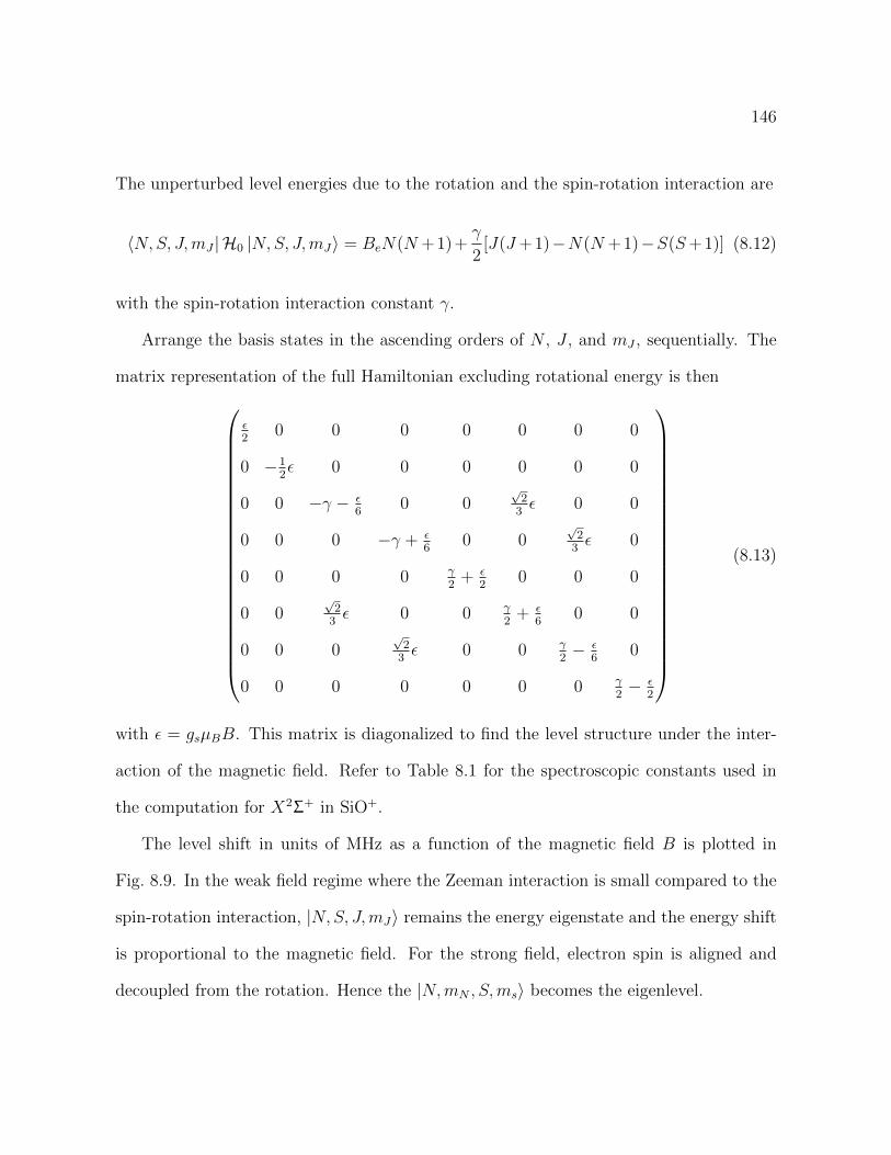
146
The unperturbed level energies due to the rotation and the spin-rotation interaction are
hN,S, J,mJ
|H0 |N,S, J,mJ
i = Be
N(N +1)+
2[J(J+1)N(N +1)S(S+1)] (8.12)
with the spin-rotation interaction constant .
Arrange the basis states in the ascending orders of N , J , and mJ
, sequentially. The
matrix representation of the full Hamiltonian excluding rotational energy is then
0
BBBBBBBBBBBBBBBBBBBBBB@
2 0 0 0 0 0 0 0
0 12 0 0 0 0 0 0
0 0
6 0 0p23 0 0
0 0 0 +
6 0 0p23 0
0 0 0 0
2 +
2 0 0 0
0 0p23 0 0
2 +
6 0 0
0 0 0p23 0 0
2
6 0
0 0 0 0 0 0 0
2
2
1
CCCCCCCCCCCCCCCCCCCCCCA
(8.13)
with = gs
µB
B. This matrix is diagonalized to find the level structure under the inter-
action of the magnetic field. Refer to Table 8.1 for the spectroscopic constants used in
the computation for X2+ in SiO+.
The level shift in units of MHz as a function of the magnetic field B is plotted in
Fig. 8.9. In the weak field regime where the Zeeman interaction is small compared to the
spin-rotation interaction, |N,S, J,mJ
i remains the energy eigenstate and the energy shift
is proportional to the magnetic field. For the strong field, electron spin is aligned and
decoupled from the rotation. Hence the |N,mN
, S,ms
i becomes the eigenlevel.

147
-500
-400
-300
-200
-100
0
100
200
300
400
0 100 200 300 400 500
Freq
uenc
y sh
ift (M
Hz)
Magnetic Field (G)
(N,J)=(1,3/2)
(1,1/2)
(0,1/2)
[mN,ms]=[1,1/2]
[1,-1/2]
[0,1/2]
[0,-1/2]
[-1,1/2]
[-1,-1/2]
[0,1/2]
[0,-1/2]
(a)
-0.4
-0.3
-0.2
-0.1
0
0.1
0.2
0.3
0.4
0 100 200 300 400 500
Sens
itivi
ty (M
Hz/
G)
Magnetic Field (G)
[0,1/2][1,1/2]
[1,-1/2]
[0,-1/2]
[0,1/2]
[0,-1/2]
[-1,-1/2][-1,1/2]
(b)
Figure 8.9. Zeeman e↵ect
Figure 8.9(b) plots the sensitivity, the derivative of the energy shift, as a function of
B. A field insensitivity transition, indicated by the red circle in the plot, can be found at
B = 214G. The corresponding transition is
0.986 |ai+ 0.169 |bi $ 0.169 |ai+ 0.986 |bi
where |ai = |N=1, J=1/2,mJ
=1/2i and |bi = |N=1, J=3/2,mJ
=1/2i. In this configu-
ration, both states have the same slope of energy shift and thus the dephasing is zero to
the first order. The second order dephasing, however, is nonzero.
Further discussion on this topic can be found in, for example, Crawford (1934).
8.5. On the Horizon
At the time this dissertation was written, the project of SiO+ was still ongoing. This
section collects some branches of this project that continue the research towards the single
ion precision spectroscopy experiment.

148
Branching Ratio / Spectroscopy
The branching times between |B, v=0i and various vibrational levels in X and A as
well as the relaxation times are crucial to the optical pumping scheme for state manipu-
lation of SiO+. While the preliminary measurement in Stollenwerk et al. (2016) provided
the fraction of the B, v0=0! X, v00=1 o↵-diagonal decay, the experiment was not sensitive
enough to measure other smaller branches such as the BA decays.
Patrick Stollenwerk is currently working on an upgraded dispersed fluorescence spec-
troscopy with trapped species. His apparatus will have a better signal-to-background
photon ratio than the previous experiment and hence will improve the detection sensitiv-
ity.
It is possible to study the time scales of the vibrational relaxation in X and the AXdecays with trapped SiO+. These measurements are usually dicult in a molecular beam
spectroscopy due to the short holding time.
Photo-dissociation
In the AlH+ cooling demonstration, the internal states are read out by REMPD.
The fidelity of the REMPD analysis is largely determined by the dissociation probability.
Recall that in the REMPD process, the molecule is first resonantly excited to an inter-
mediate state, and then subsequently photo-dissociated. However, if the dissociation step
fails (due to probability), the population is not guaranteed to decay back to its original
state. Thus, the population distribution is scrambled as REMPD is carried out with low
dissociation probability.
The dissociation probability can be calculated as the following. Let be the dissocia-
tion cross-section of a certain transition, driven by a pulsed laser with energy E per pulse

149
at wavelength . If the laser has a spot radius r, the photon number density per pulse is
E
r2hc(8.14)
where h is the Planck constant. The dissociation probability is then
P = 1 exp
E
r2hc
(8.15)
in each laser pulse.
For the AlH+ demonstration, is calculated to be 6 1018 cm2 for the dissociating
transition D2 to A2 (Seck et al., 2014). The dissociation laser, a 266 nm pulsed YAG,
has E = 2.2mJ in each pulse and the beam size is 1000 µm by 270µm. Therefore, the
dissociation probability is 99.6% per pulse, which is quite ecient.
However, for SiO+, several dissociation transitions we have considered have a low cross-
section. Figure 8.10(a) shows the REMPD cross-sections calculated by Dr. David Tabor in
his Ph.D. dissertation (Tabor, 2014). Based on the calculation, a pulsed laser with similar
energy would yield a 23% dissociation probability with a typical = 2 1019 cm2, which
is not as ecient as the case for AlH+. Figure 8.10(b) computes the single shot dissociation
probability as a function of pulse energy (in mJ) for 1mm (green), 0.5mm (orange), and
0.2mm (blue) beam radius.
If one wants to apply REMPD to SiO+, a possible solution would be applying the
laser multiple times to get a higher integrated dissociation probability. In such case, the
molecular ion is prepared in the ground rotational state, and the resonant transition in
REMPD is the quasi-closed N 0=1 ! N 00=0 transition in B-X. In principle, REMPD

150
(a) (b)
Figure 8.10. SiO+ dissociation cross-sections from B2 to (2)2 and (3)2.
may not be a useful tool for analyzing the internal state distribution, but the measured
REMPD spectrum will help improve the ab initio calculation.
Fluorescence Imaging
Direct fluorescence imaging of single isolated molecules has not yet been realized. The
challenge is mainly the low fluorescence due to the lack of closed transitions. With both
translationally and internally cold SiO+, imaging of single molecular ions may be possible
with proper repumping of the population from the X, v 6=0 and the A states. Since only a
small fraction of the fluorescence is captured, the imaging system needs to operate with
low optical aberration such that the limited amount of photons from a single ion can
focus onto one or a few pixels. Besides, the use of intensified CCD (iCCD) helps the
signal-to-noise ratio at low light level.
Precision Spectroscopy
The ultimate precision spectroscopy with single molecular ion is briefly introduced
here. The required techniques have been mostly developed in the laboratory and discussed
151
in this dissertation. The precision spectroscopy experiment will have several applications
such as testing the time-varying proton-to-electron mass ratio.
In short, a single SiO+ is co-loaded with a single Ba+ in the trap. Laser cooling of Ba+
also sympathetically cools the molecular ion to the motional ground state. The internal
state of SiO+ is cooled by the broadband rotational cooling scheme from Section 8.3. With
the population in the ground state, one can do the microwave rotational spectroscopy at
43GHz. The vibrational transition between v=0 and v=1 in X at 8 µm might be dicult
due to the laser. Next, the spectroscopy result can be read out by the motional seeding
technique from Chapter 5; the quantum logic spectroscopy technique can be performed
as well (Schmidt et al., 2005).

152
CHAPTER 9
Spectral Filtering
9.1. Introduction
The coherent broadband nature of ultrashort pulsed lasers greatly increases the band-
width of interaction between the laser and a subject. Ultrashort pulse shaping technology
further advances the degree of such interaction in many applications. For instance, in op-
tical communication, pulse shaping technology is used to encode information and perform
computation (Sardesai et al., 1998). It is also used to correct and optimize the phases of
the spectrum for generating high-quality ultrashort pulsed lasers (Pastirk et al., 2006).
In controlling chemistry, an ultrashort pulse laser with a programmed waveform provides
delicate control of molecules (Goswami, 2003; Sauer et al., 2007).
In our laboratory, we have been applying the pulse shaping technique to our molecular
rotational state cooling experiment (Lien et al., 2014, 2011). The principle of rotational
cooling is the optical pumping of transitions associated with losing rotational angular
momentum (P-branch) while avoiding those di↵using (Q-branch) or heating (R-branch)
the rotational population. This can be done by shaping a femtosecond laser’s spectrum
with a filter of which the P-branch is in the passband and the Q- and R-branch is in the
stopband, as illustrated in Fig. 9.1. The cuto↵ width of the filter determines how well
one can avoid driving an unwanted transition, and ultimately determines the molecular
cooling eciency.

153
P-branch Q-branchR-branch
Frequenc (cm–1)27,80027,70027,60027,50027,400
0
0.2
0.4
0.6
0.8
1N
orm
alize
d in
tens
ity
361363 362364360Wavelength (nm)
Figure 9.1. Rotational cooling with spectral-filtered broadband source. Inthis example, relevant transitions from A21/2, v
0=0 X21/2, v00=0 band
in the AlH+ are shown as vertical bars at the bottom. P-branch is therotational cooling transitions, while Q- and R-branch are the opposite. Anunfiltered UV femtosecond laser (spectrum shown as dashed line) drivesall transitions thus provides no cooling e↵ect. A filtered source (spectrumshown as solid line) drives only cooling transitions and hence slows downthe molecule’s rotation.
Ultrashort pulse shaping is the optical version of a waveform synthesizer. A typical
implementation is similar to an optical spectrometer. The setup first Fourier transforms
the input laser to obtain its optical spectrum with a dispersive element. Then, the an-
gularly dispersed light is focused by a lens (or a concave mirror) to map the dispersion
onto the focusing plane, where the spectrum is altered by a light modulator. Finally, the
inverse Fourier transform is performed with another set of lens and dispersive element to
form the output laser pulse with the desired spectrum or time-domain waveform.

154
High-resolution pulse shaping techniques have been the focus of ultrafast laser research
for over two decades. Usually, the pulse shaping frequency resolution is compared to
the bandwidth of the unshaped laser as the figure of merit; the ratio = / mea-
sures the number of pulse shaping control parameters. However, in our research where the
laser is used to drive transitions, it is necessary to compare to the molecular structure.
Therefore, we emphasize the absolute frequency resolution rather than the fractional. One
of the earliest pulse shaping implementations achieved 0.2 nm (51 GHz) resolution at
1064 nm (Thurston et al., 1986). For the Ti:Sapphire laser wavelength (800 nm), modu-
lation at around 0.1 nm (48 GHz) has been reported in (Monmayrant and Chatel, 2004;
Stobrawa et al., 2001). Recently, with the introduction of virtually imaged phase arrays
(VIPAs), pulse shaping reached a few GHz resolution at similar wavelength (Lee et al.,
2006; Supradeepa et al., 2008). In the UV regime, there was, however, slower progress
due to the lack of suitable light modulators. Yet, sub-nm resolution (>200 GHz) has been
demonstrated at some UV wavelengths (Weber et al., 2010). In all these experiments,
pulse shaping resolution does not necessarily include information about modulation ex-
tinction contrast. The cuto↵ feature of the amplitude modulation was seldom mentioned.
For cooling molecules with a pulse-shaped laser to work for heavier molecules such as
oxides or fluorides, resolution better than 100 GHz with high extinction ratio is required
and is the main goal of this work.
In this paper, we explore spectral filtering of a near UV femtosecond laser by providing
an introductory element-wise investigation of the setup. We first briefly review the theory
of ultrashort pulse shaping in the next section. Then, we investigate each component used
in our setup in Section 9.3. The evaluation and calibration of our spectral filtering are

155
in Section 9.4. In passing, this work is towards our molecular cooling experiment with
SiO+, for which some parameters are picked. Specifically, the relevant transitions are at
385 nm, and the rotational heating and the cooling transitions are simply separated by
an 84 GHz gap.
9.2. The Spectral Filtering Setup
Our broadband spectral filtering setup is shown in Fig. 9.2(a). The unfiltered laser
source is coupled into the setup by folding mirrors M1 and M2. Grating G1 and lens
L2 Fourier transform the light and produce the laser spectrum. Specifically, the grating
separates each spectral component into di↵erent angles. When focused by the lens, each
component becomes a spot at di↵erent locations on the focusing plane, which makes the
(optical) frequency plane. See Fig. 9.2(b). Filtering is achieved by masking the spectrum
at the plane. The filtered spectrum is recombined into a single beam by L3 and G2, which
performs the inverse Fourier transformation. The output beam is further reshaped with
a telescope (M4 and L4) to a proper size for future experiments.
The ultrashort pulse shaping technique has been greatly reviewed in several articles
including (Monmayrant et al., 2010; Weiner, 2011). Here we highlight the key results.
Consider a Gaussian input beam with 1/e2 beam radius wi
. A spectral component of
wavelength makes a focused spot with beam radius
wo
=cos
i
cos d
f
wi
(9.1)
at the frequency plane. In the above equation, f is the focal length of the lens; i
and d
are the incident and di↵raction angle at the grating, respectively. The dispersion at the

156
fs-laser WP L0 XTAL L1M1
M2
G1
G1
L2
L2
L3 Mask
G2
M3L4
h1
h1
h2
h2
h3h4
x
(a)
(b)
To Spectrometer
Figure 9.2. Schematic of our spectral filtering setup. fs-laser: mode-lockedfemtosecond laser; WP: half-wave plate; XTAL: BBO SHG crystal; L1-4:lens; M1-3: mirrors (M3 is concave). G1 and G2 are reflective di↵ractiongratings; C: fiber coupler. See text for detailed discussion.
frequency plane is
dx
d=
2f
cd cos d
(9.2)
where d is the pitch of the grating groves. The pulse shaping resolution is then the
frequency extent across the spot:
= wo
d
dx=
cd cos i
wi
. (9.3)
As a numerical example, we consider an input beam with = 385 nm and wi
= 5 mm.
We assume i
= d
10 = 49.1. With f = 500 mm lens and 2400 groves/mm grating,
the focus size is wo
= 15.6 µm and the frequency resolution is = 13.5 GHz. In this
example, the theoretical spectral filtering resolution will be sucient for the SiO+ cooling

157
experiment. The resolution is entirely set by the grating density and the input beam
size, independent to the imaging lens. However, the focus size and the dispersion are
proportional to the focal length f . If a lens with shorter f is used, the smaller spot
size becomes dicult to mask in terms of mechanical resolution. On the other hand,
using a longer f reduces the mechanical challenge but increases the setup’s footprint and
requires larger optics, which makes optical aberration become an issue. Our choice of
f = 500 mm represents a compromise between the above two concerns, along with other
matters discussed later.
The theoretical treatment of an ultrashort pulse system by the Wigner function is
a well-established method (Paye and Migus, 1995; Wefers and Nelson, 1996). On the
other hand, the response of the optics can be described by the optical transfer function
(OTF). The combination of these two thus provides the comprehensive theoretical study
of a real world pulse shaper. However, most of the previous works adopted the paraxial
approximation such that aberrations were not considered at all. Here, we only point out
but skip the theoretical investigation as it is outside the scope of our experimental work.
9.3. Setup
In this section, we introduce and comment on components in our spectral filtering
setup as well as the alignment procedure.

158
9.3.1. Light source
The input 385 nm broadband source is the second harmonic generation (SHG) of a mode-
locked femtosecond laser (Spectra Physics Mai-Tai). This is done by focusing the funda-
mental (770 nm) light with an f = 30 mm achromatic lens onto a thin (0.5 mm) BBO
crystal (Zhang et al., 1998; Ghotbi and Ebrahim-Zadeh, 2004; Ghotbi et al., 2004). The
UV beam from the crystal is collimated by a doublet lens with approximately 400 mm
e↵ective focal length. We found it is sucient to compare the beam size at near and
far fields to determine collimation. The collimated UV beam’s radius is 4.8 mm beam
horizontally and 5.7 mm vertically. The results were obtained by the knife edge beam
size measurement. The data presented an acceptable Gaussian intensity distribution.
We noticed that the UV beam acquires dispersion from the SHG process, most likely
due to the walk-o↵. We then set up the SHG such that the dispersion is aligned to the
grating’s dispersion direction, and accommodate such initial dispersion with the pulse
shaper. Further discussion continues in Section 9.3.5.
9.3.2. Grating
We use holographic gratings with 2400 groves/mm in our spectral filtering setup. These
gratings are set up in a close to Littrow configuration: the incident angle is i
= 47.1
and the di↵raction angle is d
= 40.9 at = 385 nm. While our choice of the grating
is due to component availability, a grating with higher density is of course preferred. We
would avoid ruled gratings as they are prone to periodic and irregular ruling errors that
result in ghosting and stray light and hurt the filtering resolution. However, blazed ruled

159
gratings can be more ecient; our holographic grating has about 1/2 di↵raction eciency
and is the least ecient component in the setup.
9.3.3. Focusing lens
A large aperture lens is used to accommodate the broadband light, which is a few cen-
timeters wide at L2. In such case, all types of optical aberration can be easily picked
up and makes the focus less tight. Spherical aberration is the dominant type. For tilted
incident, astigmatism is somewhat less problematic in one-dimensional pulse shaping.
Coma, on the other hand, produces a comet-like spot shape that indeed corrodes the
resolution in an asymmetric fashion. Lastly, we safely ignore chromatic aberration since
2 nm < = 385 nm. Although there is a quality spectrum of stocked optics
available from visible to IR wavelength, o↵-the-shelf optics for our application in UV is
quite limited. The option to be considered is the combining of spheric lenses into a dou-
blet lens to reduce all types of aberration mentioned above. Constructing a doublet lens
usually involves using two di↵erent glasses and optimizing the curvatures of each surface.
While we have access to only some 2” fused silica lenses, our doublet lens is constructed
by stacking a positive meniscus lens (Thorlabs LE4822) on a plano-convex lens (Thorlabs
LA4337). The e↵ective focal length of this doublet is around 500 mm.
9.3.4. Mask
The SiO+ rotational cooling requires a simple low-pass filtering mask, which is realized
by a razor blade. Installing the mask is straightforward as we place the mask at the
location where best resolution is obtained. That is, the longitudinal location of the blade

160
5 um
Sample 1
Sample 2
Sample 3
Figure 9.3. Microscope images of three samples of razor blades used inthis experiment. While we image the blades (gray area) in front of a darkbackground, the boundary between two areas is due to the blade edge. Itis easy to see the fuzziness of the blade edge is around 1 µm, smaller thanthe focal spot size ( 10 µm) in our setup.
is searched, while the transverse one is set to a specific cuto↵ frequency based on the
molecule. The knife edge is set vertically but a little tilt is not too critical as it will soften
the cuto↵ by 1/ cos , which is tiny for small tilt angle . We inspected the razor blades
under a microscope (see Fig. 9.3) and found typical edge roughness is of order 1 µm -
smaller than the focal spot size. Hence the quality of the blade edge is not yet the limiting
factor to our spectral filtering resolution. But we would avoid a used blade because of the
likely worn knife edge.
9.3.5. Dispersion compensation
The output beam acquires dispersion because the second grating G2 does not properly
recombine the filtered spectrum. The mathematical description follows. We start with

161
the grating di↵raction equation at G2:
d(sin i
+ sin d
) = . (9.4)
By expanding the above equation to the first order in i
, d
, and , we obtain the first
order dispersion:
d
=
1
d cos 0d
cos 0i
cos 0d
i
(9.5)
with
d(sin 0i
+ sin 0d
) = 0 (9.6)
being the di↵raction condition at the center wavelength 0. The term i
/ on the
right hand side of Eq. (9.5) is used to characterize the propagation of filtered spectral
components when they merge onto the grating. The output beam is dispersion-free when
d
/ = 0 and is fulfilled at a specific grating angle
0i
= cos1
1
d(
i
)1
. (9.7)
Qualitatively, Fig. 9.4 illustrates some possible scenarios. (a) is the flawless case where
the input beam has no dispersion and the optics are matched pairs. In this case, a sym-
metric 4-f line is aligned and can be reduced to a 2-f configuration by retro-reflecting the
filtered spectra at the frequency plane. In (b), the distance h1 is slightly o↵ f such that
each spectral component does not propagate in parallel between L2 and L3. This angular
error eventually results in the output beam’s dispersion if G2 is not adjusted correspond-
ingly. (c) shows the general situation where the source of error includes the input laser
already carrying dispersion and optical elements not being identical. As explained earlier,

162
G2
G2
h4G1
G1
G1
L3
L3
L3
L2
L2
L2
h=h2+h3 h1p1
(c)
(b)
h=h2+h3h4 h1
h=h2+h3h4 h1
(a)
Figure 9.4. Some possible scenarios regarding dispersion in the 4-f line.The red and the blue lines represent the propagation path of two di↵erentspectral components. (a) is an ideal case where the input beam is dispersion-free and G1=G2 and L2=L3. In (b), the alignment of some componentsis o↵, and hence the output beam derives dispersion. In general, as in (c),the source of dispersion can come from the input beam and errors fromcomponents and alignment. However, dispersion can be compensated byproperly aligning the location and the di↵raction angle of the grating G2.
the sum of all these errors is compensated by optimizing the location and the angle of the
recombining grating G2. It is worth mentioning that the input laser’s dispersion alone

163
can be corrected beforehand. Here, we simply delay that task as we can correct for some
other errors as well. Other than this aspect, the 4-f configuration is expected to have
equal performance as a 2-f configuration.
9.3.6. Alignment
We align elements in the 4-f line sequentially. After grating G1, the focusing lens L2 is
set approximately one focal length away without further optimization. The location of
L3 is adjusted such that the two lenses (L2 and L3) form a 1:1 Galilean telescope.
The recombining grating G2 should be placed where all spectral components merge; its
angle is tuned to di↵ract all components into the same direction. To check the alignment,
we use a mask with two tiny slits to select only components from both ends of the spec-
trum. We then optimize the grating until these spectral components form an overlapped
output. For example, if one sees two spots, the location of the grating needs adjustment.
Furthermore, when two spots travel at crossing paths, we know the di↵raction angle is
o↵. After G2 is optimized, the recombined output beam remains a single spot over a long
propagation distance.
9.4. Evaluation and Calibration
9.4.1. Spectrometer
In order to diagnose our spectral filtering, we also built a high-resolution spectrometer as
outlined in Fig. 9.5. The input light is coupled into the spectrometer by a single mode
fiber and is collimated to 6.8 mm beam radius. We use 3600 grooves/mm ruled grating
in our spectrometer. The focusing lens L5 is the same as the one in spectral filtering.

164
G3
L7
h5h6
CL5
L6
CCD
Figure 9.5. Schematic of our spectrometer. C: fiber output coupler; L5-6:collimation lens; G3: di↵raction grating; L7: focusing lens; CCD: linearcamera.
A linear camera is placed on the frequency plane to record the spectrum; it has 3648
pixels and each is 8 µm wide and 200 µm tall. Based on the data presented later, the
1/e2-full-width frequency resolution of this spectrometer is 28 GHz.
Our homebuilt spectrometer was also the test bed for the focusing lens. The evaluation
incorporated a narrowband CW laser to produce a single spectral component on the
frequency plane. We took this approach to check the performance of our homebuilt
doublet lens.
9.4.2. Permissible input beam size
In Fig. 9.6 we measure the profile of the focal spot for two di↵erent input beam sizes: wi
= 6.8 mm (left) and 12.1 mm (right). (The input beam size is controlled by the fiber
collimation lens.) In both cases, a compact Gaussian-like peak is observed. But the profile
due to the larger beam also has additional tails next to the central peak. As the extra

165
(a) (b)
Figure 9.6. Intensity profile on the focusing plane of a narrowband laser,recorded by a line camera. A large input beam size w
i
= 12.1 mm is usedin the right panel, and causes the focal spot to be less compact. While inthe left, a permissible beam size w
i
= 6.8 mm is used, and the focal spotprofile is fairly close to Gaussian.
feature contains non-negligible intensity, it significantly degrades the resolution even when
a larger beam is supposed to be more tightly focused. In spectral filtering, the tail results
in a low extinction cuto↵.
The origin of the tail is mostly from the transverse spherical aberration, which grows
rapidly as the cube of the aperture size. Spherical aberration limits the clear aperture
of an optics for tight focusing. From the above result, we learned that any input beam
with wi
< 6.8 mm should acquire only modest spherical aberration. Our homebuilt
doublet lens is then satisfactory in this project as the broadband UV beam size (refer to
Section 9.3.1) fits into its clear aperture.

166
9.4.3. Other aberrations
In this section, we exam the focusing behavior for spectral components that access the
lens o↵-center. A di↵erent narrowband spectral component can be obtained by changing
the wavelength of the CW laser. It, however, requires a fancy laser system to modulate
the laser wavelength over several nanometers. Therefore, to simulate tilted beams due to
di↵erent wavelengths, we rotated the grating instead. We measured the focal spot profile
for various di↵racted beam pointing in Fig. 9.7. For comparison, we performed the same
measurement with a singlet lens as well. In (a) we have the peak width on the camera
versus di↵erent tilt; in (b) some sample spot profiles at various tilts are presented. The
focal spot size stays around 16 µm over an approximately ±2 tilt with the doublet lens,
while it varies quite a lot with the singlet lens. The result shows us that we can expect
a relatively consistent resolution over the entire spectral range both in the spectrometer
and the spectral filtering setup.
From the same data we also calibrate the spectrometer’s linear dispersion. We first
read the peak locations for each tilt from Fig. 9.7(b) and fit to a straight line. Then
we computed the angular dispersion due to the grating in this spectrometer. With both
pieces of information, we obtained the calibration 7.2 GHz/pixel. In addition, the focal
spot size converts to a 14 GHz spectral resolution in our spectrometer.
9.4.4. spectral filtering
With the spectrometer and the focusing lens characterized, we now turn the attention to
the overall performance of our spectral filtering. We sent a few percent of the output light
power into our spectrometer for diagnosis. In Fig. 9.8 we see the output spectrum with

167
(a)
(b)
Figure 9.7. (a) Consistency of spectrometer resolution over its measurementrange. In this test, we simulate di↵erent narrowband laser wavelengths byrotating the grating, as if the di↵raction angle is changed due to anotherwavelength. (b) Spot profiles for data #1 (left-most), #5 (middle), and #9(right-most) from the data sequence in (a). The horizontal axis is the pixelnumber on the linear camera. The spots in the upper row are focused bythe doublet lens and those in the bottom row are focused by the singletlens. The width of each plot is 30 pixels.
(green line) and without (red line) masking. The unfiltered spectrum has a Gaussian-like
overall shape. The origin of the fringes on top of the profile is not yet clear to us. However,
we were able to see the same fringes right after the UV generation crystal, therefore our
best guess is it might come from the second harmonic generation process. Without further
168
knowledge of the fringes, we simply model the feature as a sinusoidal modulation to the
Gaussian function:
A exp
(
c
)2
1 + h sin
2( p
)
(9.8)
where c
is the broadband laser center frequency, is the laser bandwidth, is the
fringe period, p
is used to adjust the fringe’s o↵set, and h is the modulation index.
The unfiltered spectrum has = 7.1 THz full-width-half-maximum bandwidth, and the
period of the fringes is around = 150 GHz.
For the cuto↵, we model it with an error function
g(, 0) = g( 0) =1
2[erf(
0p2
) + 1] (9.9)
where 0 is the cuto↵ frequency and is the cuto↵ width. Positive represents a
high-pass mask and negative is low-pass. The error function is a natural choice in our
analysis as the edge of the mask partially blocks a Gaussian beam. Fig. 9.8(b) shows
a typical filtered spectrum near the cuto↵ with our model applied to the data. In this
demonstration, the cuto↵ width is 48 GHz. Compared to the expected di↵raction-
limited resolution, this result is 33% worse.
In Fig. 9.9 we measure the width for di↵erent mask longitudinal locations z. The
result is modeled by
(z) = 0
r1 + (
z z0zR
)2 (9.10)
which resembles the equation for Gaussian beam width evolution. The range zR
=
±11.2 mm is considered the alignement tolerance of the mask.
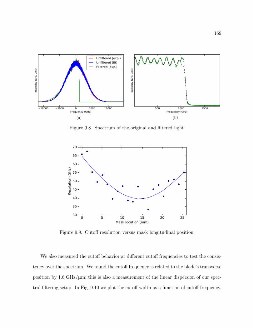
169
(a) (b)
Figure 9.8. Spectrum of the original and filtered light.
Figure 9.9. Cuto↵ resolution versus mask longitudinal position.
We also measured the cuto↵ behavior at di↵erent cuto↵ frequencies to test the consis-
tency over the spectrum. We found the cuto↵ frequency is related to the blade’s transverse
position by 1.6 GHz/µm; this is also a measurement of the linear dispersion of our spec-
tral filtering setup. In Fig. 9.10 we plot the cuto↵ width as a function of cuto↵ frequency.

170
Figure 9.10. cuto↵ resolution versus di↵erent cuto↵ frequency.
We notice that the cuto↵ width varies rapidly across the laser spectrum, and the varia-
tion coincides with the spectral fringes from the unfiltered light, shown in the gray line.
As we currently have no plausible explanation for the fringes, we cannot understand the
correlation either. Regardless, by eye-averaging the result, we find the cuto↵ resolution is
worsened by around 20% when away from the central wavelength, which can be attributed
to the optical aberration.
9.5. Improvement
We have demonstrated that the focusing lens is the key component in both the spec-
trometer and the spectral filtering setup. In this project, we used standard optics com-
ponents available from common vendors, which significantly limited the ability of aber-
ration correction. The immediate also less expensive solution is to build a doublet lens
with proper choices of lens materials and surface curvatures. By doing optical ray tracing

171
simulations, we, however, found that, for doublet lenses utilizing spherical surfaces, the
largest clear aperture diameter is somehow around 20 mm. The performance seems to be
limited by the number of tuning variables in lens design. That is, if one wants to work
with larger input beam size, it is necessary to use aspheric optics.
The input beam shape is another factor that might need more studying. While SHG of
a femtosecond laser is quite simple, we have observed evidence of beam shape degradation.
The obvious one is astigmatism where the UV beam presents an elliptical shape. In
addition, the UV beam is accompanied by a halo; it is not clear to us how this scattered
light behaves in the pulse shaping setup and a↵ects the filtering resolution.
To ultimately reach close to the di↵raction limit, wavefront distortion caused by, e.g.,
optics surface irregularity, is yet another obstacle to be studied and overcome.
Finally, regarding the mask, a razor blade serves as an adequate bandpass filter for our
molecular cooling experiment. For comprehensive modulation, a spatial light modulator
(SLM) is a better option. SLMs with good resolution and dynamic range have become
available in the UV band. Options to be considered for our future experiment include
liquid crystal (Tanigawa et al., 2009), acousto-optic modulator (Roth et al., 2005; Pearson
and Weinacht, 2007), and micro-mirror array (Rondi et al., 2009).

172
References
Agap’ev, B. D., M. B. Gornyı, B. G. Matisov, and Y. V. Rozhdestvenskiı (1993), Physics-Uspekhi 36 (9), 763.
Appelhans, A. D., and D. A. Dahl (2002), Int. J. Mass. Spectrom. 216 (3), 269.
Arnesen, A., A. Bengtsson, R. Hallin, S. Kandela, T. Noreland, and R. Lidholt (1975),Phys. Lett. A 53 (6), 459.
Arroe, O. (1950), Phys. Rev. 79 (5), 836.
Bahns, J., W. Stwalley, and P. Gould (1996), J. Chem. Phys. 104 (24), 9689.
Berkeland, D. J., J. D. Miller, J. C. Bergquist, W. M. Itano, and D. J. Wineland (1998),J. Appl. Phys. 83 (10), 5025.
Biercuk, M. J., H. Uys, J. W. Britton, A. P. VanDevender, and J. J. Bollinger (2010),Nat. Nanotechnol. 5 (9), 646.
Bohme, D. K. (1990), Int. J. Mass. Spectrom. 100, 719.
Brown, J. M., and A. Carrington (2003), Rotational Spectroscopy of Diatomic Molecules(Cambridge University Press).
Cai, Z. L., and J. P. Francois (1999), J. Mol. Spectrosc. 197 (1), 12.
Cameron, R., T. Scholl, L. Zhang, R. Holt, and S. Rosner (1995a), J. Mol. Spectrosc.169 (2), 352.
Cameron, R., T. J. Scholl, L. Zhang, R. A. Holt, and S. D. Rosner (1995b), J. Mol.Spectrosc. 169 (2), 364.
Chattopadhyaya, S., A. Chattopadhyay, and K. K. Das (2003), J. Mol. Struc.-Theochem639 (1), 177.
Chen, X., Y. Lin, and B. Odom (2015), New J. Phys. 17 (4), 043037.

173
Chieda, M., and E. Eyler (2011), Phys. Rev. A 84 (6), 063401.
Chou, C., D. Hume, J. Koelemeij, D. Wineland, and T. Rosenband (2010), Phys. Rev.Lett. 104 (7), 070802.
Clark, C. R., J. E. Goeders, Y. K. Dodia, C. R. Viteri, and K. R. Brown (2010), Phys.Rev. A 81 (4), 043428.
Colbourn, E., J. Dyke, E. Lee, A. Morris, and I. Trickle (1978), Mol. Phys. 35 (3), 873.
Crawford, F. (1934), Rev. Mod. Phys. 6 (2), 90.
Curry, J. (2004), J. Phys. Chem. Ref. Data 33 (3), 725.
Davidson, M., L. Snoek, H. Volten, and A. Donszelmann (1992), Astron. Astrophys. 255,457.
Ding, S., and D. Matsukevich (2012), New J. Phys. 14 (2), 023028.
Doroshenko, V. M., and R. J. Cotter (1997), J. Mass. Spectrom. 32 (6), 602.
Drewsen, M., A. Mortensen, R. Martinussen, P. Staanum, and J. L. Sørensen (2004),Phys. Rev. Lett. 93 (24), 243201.
Dzuba, V., and J. Ginges (2006), Phys. Rev. A 73 (3), 032503.
Fahey, D., F. Fehsenfeld, E. Ferguson, and L. Viehland (1981), J. Chem. Phys. 75 (2),669.
Flambaum, V., and A. Tedesco (2006), Phys. Rev. C 73 (5), 055501.
Ghosh, P. (1995), Ion traps (Clarendon Press; Oxford (United Kingdom)).
Ghosh, S., J. V. der Linde, and R. Verma (1979), J. Mol. Spectrosc. 75 (2), 169 .
Ghotbi, M., and M. Ebrahim-Zadeh (2004), Opt. Express. 12 (24), 6002.
Ghotbi, M., M. Ebrahim-Zadeh, A. Majchrowski, E. Michalski, and I. Kityk (2004), Opt.Lett. 29 (21), 2530.
Godun, R., P. Nisbet-Jones, J. Jones, S. King, L. Johnson, H. Margolis, K. Szymaniec,S. Lea, K. Bongs, and P. Gill (2014), Phys. Rev. Lett. 113 (21), 210801.
Goldfarb, R. B., and H. E. Bussey (1987), Rev. Sci. Instrum. 58 (4), 624.

174
Goswami, D. (2003), Phys. Rep. 374 (6), 385.
Grimm, R., Y. B. Ovchinnikov, A. I. Sidorov, and V. S. Letokhov (1990), Phys. Rev.Lett. 65 (12), 1415.
Gurell, J., E. Biemont, K. Blagoev, V. Fivet, P. Lundin, S. Mannervik, L.-O. Norlin,P. Quinet, D. Rostohar, P. Royen, et al. (2007), Phys. Rev. A 75 (5), 052506.
Horowitz, P., W. Hill, and I. Robinson (1980), The art of electronics, Vol. 1989 (Cam-bridge university press Cambridge).
Hume, D. B., C. W. Chou, D. R. Leibrandt, M. J. Thorpe, D. J. Wineland, and T. Rosen-band (2011), Phys. Rev. Lett. 107 (24), 10.1103/PhysRevLett.107.243902.
Hunt, F. J. (1976), J. Phys. E 9 (11), 921.
Ibaraki, Y., U. Tanaka, and S. Urabe (2011), Appl. Phys. B 105 (2), 219.
Jadraque, M., M. Santos, L. Dıaz, J. Alvarez-Ruiz, and M. Martın (2009), J. Phys. Chem.A 113 (41), 10880.
Kaplan, A. E. (2009), Opt. Express. 17 (12), 10035.
Knunz, S., M. Herrmann, V. Batteiger, G. Saatho↵, T. Hansch, K. Vahala, and T. Udem(2010), Phys. Rev. Lett. 105 (1), 013004.
Kokish, M., M. Dietrich, and B. Odom (2016), J. Phys. B 49 (3), 035301.
Lagerqvist, A., and I. Renhorn (1974), J. Mol. Spectrosc. 49 (1), 157.
Latawiec, A., and G. Lockwood (1966), “Method of electropolishing tungsten wire,” USPatent 3,287,238.
Lee, G.-H., S. Xiao, and A. M. Weiner (2006), IEEE Photonic Tech. L. 18 (17), 1819.
Leibfried, D. (2012), New J. Phys. 14 (2), 023029.
Leibfried, D., R. Blatt, C. Monroe, and D. Wineland (2003), Rev. Mod. Phys. 75 (1),281.
Lien, C.-Y., C. M. Seck, Y.-W. Lin, J. H. V. Nguyen, D. A. Tabor, and B. C. Odom(2014), Nat. Commun. 5.

175
Lien, C.-Y., S. R. Williams, and B. Odom (2011), J. Chem. Phys. 13 (42), 18825.
Lin, Y.-W., S. Williams, and B. Odom (2013), Phys. Rev. A 87 (1), 011402.
Lindberg, M., and J. Javanainen (1986), JOSA B 3 (7), 1008.
Macalpine, W., and R. Schildknecht (1959), Proceedings of the IRE 47 (12), 2099.
Marzoli, I., J. Cirac, R. Blatt, and P. Zoller (1994), Phys. Rev. A 49 (4), 2771.
Matsuo, Y., T. Nakajima, T. Kobayashi, and M. Takami (1997), Appl. Phys. Lett. 71,996.
Mogi, T., Y. Fukuyama, T. Kobayashi, I. Tanihata, K. Uehara, and Y. Matsuo (2002),Appl. Surf. Sci. 197, 202.
Monmayrant, A., and B. Chatel (2004), Rev. Sci. Instrum. 75, 2668.
Monmayrant, A., S. Weber, and B. Chatel (2010), J. Phys. B 43 (10), 103001.
Muller, B., and C. Ottinger (1986), J. Chem. Phys. 85 (1), 232.
Mur-Petit, J., J. J. Garcıa-Ripoll, J. Perez-Rıos, J. Campos-Martınez, M. I. Hernandez,and S. Willitsch (2012), Phys. Rev. A 85 (2), 022308.
Nakamura, K. G., I. Kamioka, and M. Kitajima (1996), J. Chem. Phys. 104 (9), 3403.
Nakamura, K. G., and M. Kitajima (1994), Appl. Phys. Lett. 65 (19), 2445.
Nakamura, K. G., and M. Kitajima (1995), J. Chem. Phys. 102 (21), 8569.
Nguyen, J., and B. Odom (2011), Phys. Rev. A 83 (5), 053404.
Nguyen, J. H., C. R. Viteri, E. G. Hohenstein, C. D. Sherrill, K. R. Brown, and B. Odom(2011), New J. Phys. 13 (6), 063023.
Oddershede, J., and N. Elander (1976), J. Chem. Phys. 65 (9), 3495.
Ott, G., J. Wrba, and R. Lucke (2003), J. Magn. Magn. Mater. 254, 535.
Pankhurst, R. (1940), P. Phys. Soc. 52 (5), 707.
Pastirk, I., B. Resan, A. Fry, J. MacKay, and M. Dantus (2006), Opt. Express. 14 (20),9537.

176
Paye, J., and A. Migus (1995), JOSA B 12 (8), 1480.
Pearson, B. J., and T. C. Weinacht (2007), Opt. Express. 15 (7), 4385.
Rondi, A., J. Extermann, L. Bonacina, S. Weber, and J.-P. Wolf (2009), Appl. Phys. B96 (4), 757.
Rosenband, T., D. Hume, P. Schmidt, C. Chou, A. Brusch, L. Lorini, W. Oskay,R. Drullinger, T. Fortier, J. Stalnaker, et al. (2008), Science 319 (5871), 1808.
Rosner, S., R. Cameron, T. Scholl, and R. Holt (1998), J. Mol. Spectrosc. 189 (1), 83.
Roth, M., M. Mehendale, A. Bartelt, and H. Rabitz (2005), Appl. Phys. B 80 (4-5), 441.
Sardesai, H., C.-C. Chang, and A. Weiner (1998), Journal of Lightwave Technology16 (11), 1953.
Sauer, F., A. Merli, L. Woste, and A. Lindinger (2007), J. Chem. Phys. 334 (1), 138.
Schmidt, P. O., T. Rosenband, J. C. J. Koelemeij, D. B. Hume, W. M. Itano, J. C.Bergquist, and D. J. Wineland (2006), Non-Neutral Plasma Physics VI, Aip Confer-ence Proceedings, 862, 305.
Schmidt, P. O., T. Rosenband, C. Langer, W. M. Itano, J. C. Bergquist, and D. J.Wineland (2005), Science 309 (5735), 749.
Scholl, T., R. Cameron, S. Rosner, and R. Holt (1995), Phys. Rev. A 51 (3), 2014.
Schuessler, H. A., and O. Chun-Sing (1981), Nucl. Instrum. Methods 186 (1), 219.
Schwartz, J. C., M. W. Senko, and J. E. Syka (2002), J. Am. Soc. Mass. Spectr. 13 (6),659.
Seck, C. M., E. G. Hohenstein, C.-Y. Lien, P. R. Stollenwerk, and B. C. Odom (2014),J. Mol. Spectrosc. 300, 108.
Seck, C. M., M. G. Kokish, M. R. Dietrich, and B. C. Odom (2016), Phys. Rev. A 93 (5),053415.
Shelkovnikov, A., R. J. Butcher, C. Chardonnet, and A. Amy-Klein (2008), Phys. Rev.Lett. 100 (15), 150801.
Sheridan, K., and M. Keller (2011), New J. Phys. 13 (12), 123002.

177
Sheridan, K., N. Seymour-Smith, A. Gardner, and M. Keller (2012), Eur. Phys. J. D66 (11), 1.
Shi, D., W. Li, W. Xing, J. Sun, Z. Zhu, and Y. Liu (2012), Computational and Theo-retical Chemistry 980, 73.
Shu, G., N. Kurz, M. Dietrich, and B. Blinov (2010), Phys. Rev. A 81 (4), 042321.
Siverns, J., L. Simkins, S. Weidt, and W. Hensinger (2012), Appl. Phys. B 107 (4), 921.
Staanum, P. F., K. Højbjerre, P. S. Skyt, A. K. Hansen, and M. Drewsen (2010), Nat.Phys. 6 (4), 271.
Steele, A., L. Churchill, P. Grin, and M. Chapman (2007), Phys. Rev. A 75 (5), 053404.
Stenholm, S. (1986), Rev. Mod. Phys. 58 (3), 699.
Stobrawa, G., M. Hacker, T. Feurer, D. Zeidler, M. Motzkus, and F. Reichel (2001),Appl. Phys. B 72 (5), 627.
Stollenwerk, P. R., B. C. Odom, D. L. Kokkin, and T. Steimle (2016), J. Mol. Spectrosc..
Streed, E. W., B. G. Norton, A. Jechow, T. J. Weinhold, and D. Kielpinski (2011), Phys.Rev. Lett. 106 (1), 010502.
Sturm, S., F. Kohler, J. Zatorski, A. Wagner, Z. Harman, G. Werth, W. Quint, C. H.Keitel, and K. Blaum (2014), Nature 506 (7489), 467.
Supradeepa, V., C.-B. Huang, D. E. Leaird, and A. M. Weiner (2008), Opt. Express16 (16), 11878.
Tabor, D. (2014), Toward Rotational Cooling of Trapped SiO+ by Optical Pumping, Ph.D.thesis (Northwestern University).
Tabor, D., V. Rajagopal, Y.-W. Lin, and B. Odom (2012), Appl. Phys. B 107 (4), 1097.
Tanigawa, T., Y. Sakakibara, S. Fang, T. Sekikawa, and M. Yamashita (2009), Opt. Lett.34 (11), 1696.
Thurston, R., J. Heritage, A. Weiner, and W. Tomlinson (1986), IEEE J. Quantum Elect.22 (5), 682.

178
Torres, R., M. Jadraque, and M. Martin (2005), Appl. Phys. A 80 (8), 1671.
Ubachs, W., J. Bagdonaite, E. J. Salumbides, M. T. Murphy, and L. Kaper (2016), Rev.Mod. Phys. 88, 021003.
Uzan, J.-P. (2011), Living Rev. Relativity 14 (2).
Vahala, K., M. Herrmann, S. Knuenz, V. Batteiger, G. Saatho↵, T. W. Haensch, andT. Udem (2009), Nat. Phys. 5 (9), 682.
Vanhaecke, N., and O. Dulieu (2007), Mol. Phys. 105 (11-12), 1723.
Villemoes, P., A. Arnesen, F. Heijkenskjold, and A. Wannstrom (1993), J. Phys. B26 (22), 4289.
Viteau, M., A. Chotia, M. Allegrini, N. Bouloufa, O. Dulieu, D. Comparat, and P. Pillet(2008), Science 321 (5886), 232.
Vizmuller, P. (1995), RF design guide: systems, circuits, and equations, Vol. 1 (ArtechHouse).
Voitsekhovich, V. S., M. V. Danileiko, A. M. Negriiko, V. I. Romanenko, and L. P.Yatsenko (1989), JETP Lett. 49 (3), 161.
Wang, B., J. Zhang, C. Gao, and L. Wang (2011), Opt. Express. 19 (17), 16438.
Watson, J. K. (2008), J. Mol. Spectrosc. 252 (1), 5.
Weber, S., M. Barthelemy, and B. Chatel (2010), Appl. Phys. B 98 (2-3), 323.
Wefers, M. M., and K. A. Nelson (1996), IEEE J. Quantum Elect. 32 (1), 161.
Weiner, A. M. (2011), Opt. Commun. 284 (15), 3669 , special Issue on Optical PulseShaping, Arbitrary Waveform Generation, and Pulse Characterization.
Welling, M., H. Schuessler, R. Thompson, and H. Walther (1998), Int. J. Mass. Spectrom.172 (1), 95.
Wendt, K., S. Ahmad, F. Buchinger, A. Mueller, R. Neugart, and E.-W. Otten (1984),Zeitschrift fur Physik A Atoms and Nuclei 318 (2), 125.
Wineland, D., W. M. Itano, J. Bergquist, and R. G. Hulet (1987), Phys. Rev. A 36 (5),2220.

179
Wineland, D. J., and W. M. Itano (1979), Phys. Rev. A 20 (4), 1521.
Wineland, D. J., C. Monroe, W. M. Itano, D. Leibfried, B. E. King, and D. M. Meekhof(1997), arXiv preprint quant-ph/9710025 .
Woods, L. (1943), Phys. Rev. 63 (11-12), 426.
Zhang, C. B., D. O↵enberg, B. Roth, M. Wilson, and S. Schiller (2007), Phys. Rev. A76 (1), 012719.
Zhang, J.-y., J. Y. Huang, H. Wang, K. Wong, and G. Wong (1998), JOSA B 15 (1),200.
Zverev, A. I. (1967), Handbook of filter synthesis (Wiley-Blackwell).
addtocontentslof

180
APPENDIX A
Fluorescence from a Three-level System
Here I consider the population cycling in a three-level system: a is the excitation, b
and c are the two ground states. The a!c decay is assumed to to weaker than a!b;
therefore a! b is the fluorescing transition and a! c is the repumping transition. The
Optical Bloch equation of the system is:
0ab
= (b
+ c
2 i
b
)ab
+ i
b
2(
a
b
) i
c
2cb
(A.1a)
0ba
= (b
+ c
2+ i
b
)ba
i
b
2(
a
b
) + i
c
2bc
(A.1b)
0ac
= (b
+ c
2 i
c
)ac
+ i
c
2(
a
c
) i
b
2bc
(A.1c)
0ca
= (b
+ c
2+ i
c
)ca
i
c
2(
a
c
) + i
b
2cb
(A.1d)
0cb
= i(c
b
)cb
+ i
b
2ca
i
c
2ab
(A.1e)
0bc
= i(b
c
)bc
i
b
2ac
+ i
c
2ba
(A.1f)
0b
= ib
2(
ab
ba
) + b
a
(A.1g)
0c
= ic
2(
ac
ca
) + c
a
(A.1h)
a
+ b
+ c
= 1. (A.1i)
In these equations, b,c
, b,c
, and b,c
are the spontaneous emission rates, Rabi frequen-
cies, and the detunings for the a$ b and a$ c transitions, respectively. Because the two
181
light sources are incoherent, coherence between b and c vanishes. By taking bc
= cb
= 0,
we obtain the following equations for steady state:
(b
+ c
2 i
b
)ab
+ i
b
2(
a
b
) = 0 (A.2a)
(b
+ c
2+ i
b
)ba
i
b
2(
a
b
) = 0 (A.2b)
(b
+ c
2 i
c
)ac
+ i
c
2(
a
c
) = 0 (A.2c)
(b
+ c
2+ i
c
)ca
i
c
2(
a
c
) = 0 (A.2d)
ib
2(
ab
ba
) + b
a
= 0 (A.2e)
ic
2(
ac
ca
) + c
a
= 0 (A.2f)
a
+ b
+ c
= 1. (A.2g)
To simplify the expression, introduce
Fb,c
=(
b,c
/)2
(b,c
/)[1 + (2b,c
/)2] + (b,c
/)2(A.3)
where = b
+ c
is the total spontaneous emission rate. Note that the value of Fb,c
takes place between 0 and 1. The solution of the population terms is
a
= Fb
Fc
/(Fb
Fc
+ Fc
+ Fb
) (A.4a)
b
= Fc
/(Fb
Fc
+ Fc
+ Fb
) (A.4b)
c
= Fb
/(Fb
Fc
+ Fc
+ Fb
) (A.4c)

182
and the solution of the coherence terms is
ab
=i(1 + 2i
b
/)(b
/)
(b
/)[1 + (2b
/)2] + (b
/)2
b
(A.4d)
ac
=i(1 + 2i
c
/)(c
/)
(c
/)[1 + (2c
/)2] + (c
/)2
c
. (A.4e)
The fluorescence rate is proportional to the excitation state population a
. It is easy
to see that a
is monotonic in both Fb
and Fc
once we rearrange Eq. A.4b as
a
=Fb
Fc
Fb
+ Fc
+ Fb
Fc
=1
1 + 1/Fb
+ 1/Fc
. (A.5)
The maximum value of a
is 1/3 when Fb
= Fc
= 1. Fig. A.1 upper plot shows Fc
as a
function of c
/c
for various c
/b
. The lower plot shows the dependence between the
excitation state population a
and the repumping intensity. For a weaker transition, we
will need much stronger intensity to provide sucient repumping.
Einstein’s Rate Equation
It is interesting to study the rate equation formulation to model the population dy-
namics in the same three-level system as well:
0a
= (b
+ c
)a
+ ub
Bb
b
ub
Bb
a
+ uc
Bc
c
uc
Bc
a
(A.6a)
0b
= b
a
ub
Bb
b
+ ub
Bb
a
(A.6b)
0c
= c
a
uc
Bc
c
+ uc
Bc
a
(A.6c)
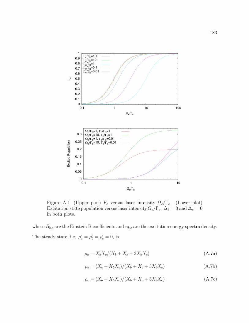
183
0 0.1 0.2 0.3 0.4 0.5 0.6 0.7 0.8 0.9
1
0.1 1 10 100
F c
Ωc/Γc
Γc/Γb=100Γc/Γb=10Γc/Γb=1Γc/Γb=0.1Γc/Γb=0.01
0
0.05
0.1
0.15
0.2
0.25
0.3
0.1 1 10
Exci
ted
Popu
latio
n
Ωc/Γc
Ωb/Γb=1, Γc/Γb=1Ωb/Γb=10, Γc/Γb=1Ωb/Γb=1, Γc/Γb=0.01Ωb/Γb=10, Γc/Γb=0.01
Figure A.1. (Upper plot) Fc
versus laser intensity c
/c
. (Lower plot)Excitation state population versus laser intensity
c
/c
. b
= 0 andc
= 0in both plots.
where Bb,c
are the Einstein B coecients and ub,c
are the excitation energy spectra density.
The steady state, i.e. 0a
= 0b
= 0c
= 0, is
a
= Xb
Xc
/(Xb
+Xc
+ 3Xb
Xc
) (A.7a)
b
= (Xc
+Xb
Xc
)/(Xb
+Xc
+ 3Xb
Xc
) (A.7b)
c
= (Xb
+Xb
Xc
)/(Xb
+Xc
+ 3Xb
Xc
) (A.7c)

184
with Xb,c
= ub,c
Bb,c
/b,c
. To relate the Einstein rate equation to Optical Bloch equation,
we compare Eq. A.1g and A.1h to Eq. A.6b and A.6c. The A coecients are just
the spontaneous emission rate: Ab,c
= b,c
. The stimulated absorption/emission terms
between state a and b (or c) in the Optical Bloch equations can be written as
ib,c
2(
ab,c b,ca) =1
1 + (2b,c
/)22
b,c
(
a
b,c
). (A.8)
Compare to the corresponding terms in the rate equation we find the expression for
stimulated transition rate with monochromatic drive to be
ub,c
Bb,c
=1
1 + (2b,c
/)22
b,c
. (A.9)
Furthermore, we find
Fb,c
=X
b,c
1 +Xb,c
(A.10)
and Eq. A.7a becomes
a
=X
b
Xc
Xb
+Xc
+ 3Xb
Xc
(A.11)
=1
1/Xb
+ 1/Xc
+ 3
=1
1 + 1/Fb
+ 1/Fc
,
which is identical to Eq. A.5.

185
How About the Broadband Source?
The expression in Eq. A.9 is for a monochromatic light source. The result can be
rewritten as a function of laser intensity:
uc
Bc
=1
1 + (2c
/)22c
I
2Is
(A.12)
where Is
= hcc
/33 is the saturation intensity. We describe a broadband source with
a normalized spectra function g(!):
I()! P
Ag()d
where P is the total power and A is the beam size. The stimulated transition rate is then
generalized as
uc
Bc
=
Z1
1 + (2c
/)22c
P/A
2Is
g(c
)dc
. (A.13)
As an example, we consider a source with constant spectra density g() = 1/w over a
bandwidth w. We then have
uc
Bc
=2c
P/Aw
2Is
Zw/2
w/2
dc
1 + (2c
/)2=
2c
P
2AIs
tan1(w/)
w. (A.14)
The case of w ! 0 gives the result for a resonant monochromatic source. When w
the rate becomes
uc
Bc
=c
2Is
Pc
2Aw=
c
3P3
4hcAw. (A.15)

186
APPENDIX B
Finite Element Analysis of the Trap Potential
The appendix provides the technical supplementary to Section 2.2 by listing the sim-
ulation scripts.
Set up the Mesh
First, the geometry of the trap is scripted in a ”.geo” file. Then Gmsh discretizes the
geometry and creates a ”.msh” mesh file by the following command.
gmsh 3 <input . geo> o <output .msh>
FreeFem++
To solve the di↵erential equation by FreeFem++, another script ”.edp” files is created
with information of the equation, boundaries, and solver options. A sample script is
attached below.
1 // Load nece s sa ry packagesload ”gmsh”load ”medit”load ”MUMPS”
5
// Load mesh f i l emesh3 Th = gmshload3 (” t r a p s i n g l e .msh”) ;
// Create the f i n i t e element space10 f e spac e Vh(Th, P13d ) ;
Vh uh=x+y+z , vh ;

187
// Def ine g rad i en tmacro Grad (u) [ dx (u) , dy (u) , dz (u) ] //
15 // A l l o ca t e an array f o r boundary va lue sr e a l [ i n t ] bc (4 ) ;
// Set up the Laplace equat ion as we l l as the boundary,! cond i t i on s
problem Lap(uh , vh ) = int3d (Th) (Grad (uh) ’Grad (vh ) )20 + on (800 , uh=bc [ 0 ] ) // conta ine r
+ on (801 , uh=bc [ 1 ] ) + on (802 , uh=bc [ 2 ] ) // r f,! rods
+ on (803 , uh=bc [ 3 ] ) ; // end caps
// Solve the problem and save the answer to a f i l e25 cout << ”1 : 801” << endl ;
// One o f the boundar ies va lue i s s e t to 1bc = 0 ;bc [ 1 ] = 1 ;// Solve
30 Lap ;// Output to f i l e
ofstream f f (” ans 801 . txt ”) ;f o r ( i n t i =0; i<Vh. ndof ; i++)
35 f f << Th( i ) . x << ” ” << Th( i ) . y << ” ” << Th,! ( i ) . z << ” ” << uh [ ] [ i ] << endl ;
To solve the problem, execute the following command.
FreeFem++ <s c r i p t . edp>
Note that both Gmsh and FreeFem++ have a GUI interface and the job can certainly
be done by using the GUI. However, be careful that the computer eciency may quite
reduced as visualization of the complex geometry would use lots of resource. Therefore,
using GUI is not recommended.

188
Post-processing
A sample python script for the multipole expansion fitting is attached below.
1 import numpy as npimport s c ipy . s p e c i a l
import matp lo t l i b5 import matp lo t l i b . mlab as mlabimport matp lo t l i b . cm as cmimport matp lo t l i b . pyplot as p l t
de f yLegSphHarm( l , m) :10 q = np . power ( r2 , l /2) s c ipy . s p e c i a l . lpmv (m, l , c t )
i f m==0:re turn q
e l i f m>0:r e turn qnp . cos (mphi )
15 e l s e :r e turn qnp . s i n (mphi )
de f makeAMatrix ( lmax ) :20 A = np . ones ( l en (x ) )
f o r l in range (2 , lmax+1 ,2) :A = np . c [A, yLegSphHarm( l , 0 ) ]f o r m in range (2 , l +1 ,2) :
A = np . c [A, yLegSphHarm( l ,m) ,,! yLegSphHarm( l ,m) ]
25 r e turn A
data = np . l oadtx t ( ’ a n s s i n g l e 8 0 1 . txt ’ )x = data [ : , 0 ]
30 y = data [ : , 1 ]z = data [ : , 2 ]v = data [ : , 3 ]
pIdx = np . f l a t non z e r o ( ( ( xx+yy ) <0.22)&(abs ( z ) <0.8) )35
x = x [ pIdx ]

189
y = y [ pIdx ]z = z [ pIdx ]v = v [ pIdx ]
40
r2 = xx+yy+zzr = np . sq r t ( r2 )ct = [ z1/ r1 i f r1>0 e l s e 0 . 0 f o r z1 , r1 in z ip ( z , r ) ]
45 phi = np . arctan2 (y , x )
A = makeAMatrix (8 )(U, w, V) = np . l i n a l g . svd (A, f u l l m a t r i c e s=Fal se )
50 b = np . dot ( ( np . dot (U.T, v ) /w) , V)s = np . sq r t (np . dot (V.T2 ,1/w2) )
b1 = [ ’%.2 e ’ % e l e f o r e l e in b ]
55
# pr in t (np . l i n a l g . norm(A. dot (b)v ) )
de f legSphHarm ( l , m, x , y , z ) :r2 = xx+yy+zz
60 ct = z/np . s q r t ( r2 ) i f r2 !=0 e l s e 0 . 0q = np . power ( r2 , l /2) s c ipy . s p e c i a l . lpmv (m, l , c t )i f m==0:
re turn qe l i f m>0:
65 r e turn qnp . cos (mnp . arctan2 (y , x ) )e l s e :
r e turn qnp . s i n (mnp . arctan2 (y , x ) )
de f comp( lMax , x , y , z ) :70 p = np . array ( [ 1 ] )
f o r l in range (2 , lMax+1 ,2) :p = np . append (p , legSphHarm ( l , 0 , x , y , z ) )f o r m in range (2 , l +1 ,2) :
p = np . append (p , [ legSphHarm ( l , m, x,! , y , z ) , legSphHarm ( l , m, x ,,! y , z ) ] )
75 r e turn p

190
# np . dot (b , comp ( ) ) g i v e s the f i t t i n g r e s u l t
B.1. Single Ion Trap
Trap Geometry
1 Mesh . VolumeEdges = 0 ;
Macro yC i r c l ep0 = newp ; Point ( p0 ) = x0 , y0 , z0 ;
5 p1 = newp ; Point ( p1 ) = x0+r , y0 , z0 ;p2 = newp ; Point ( p2 ) = x0 , y0+r , z0 ;p3 = newp ; Point ( p3 ) = x0r , y0 , z0 ;p4 = newp ; Point ( p4 ) = x0 , y0r , z0 ;Cha r a c t e r i s t i c Length p1 , p2 , p3 , p4 = l c ;
10 c1 = newreg ; C i r c l e ( c1 ) = p1 , p0 , p2 ;c2 = newreg ; C i r c l e ( c2 ) = p2 , p0 , p3 ;c3 = newreg ; C i r c l e ( c3 ) = p3 , p0 , p4 ;c4 = newreg ; C i r c l e ( c4 ) = p4 , p0 , p1 ;l l = newreg ; Line Loop ( l l ) = c1 , c2 , c3 , c4 ;
15 Return
Macro Cyl inderCa l l yC i r c l e ;s1 = newreg ; Plane Sur face ( s1 ) = l l ;
20 out [ ] = Extrude 0 , 0 , L Sur face s1 ; ;De lete Volumeout [ 1 ] ; out [ 1 ] = out [ 0 ] ; out [ 0 ] = s1 ;
Return
25
// parametersinch = 25 . 4 ;
// Container30 x0 = 0 ; y0 = 0 ; z0 = 2.2;
r = 2 ; L = 4 . 4 ; l c = 0 . 2 ;Ca l l Cyl inder ;
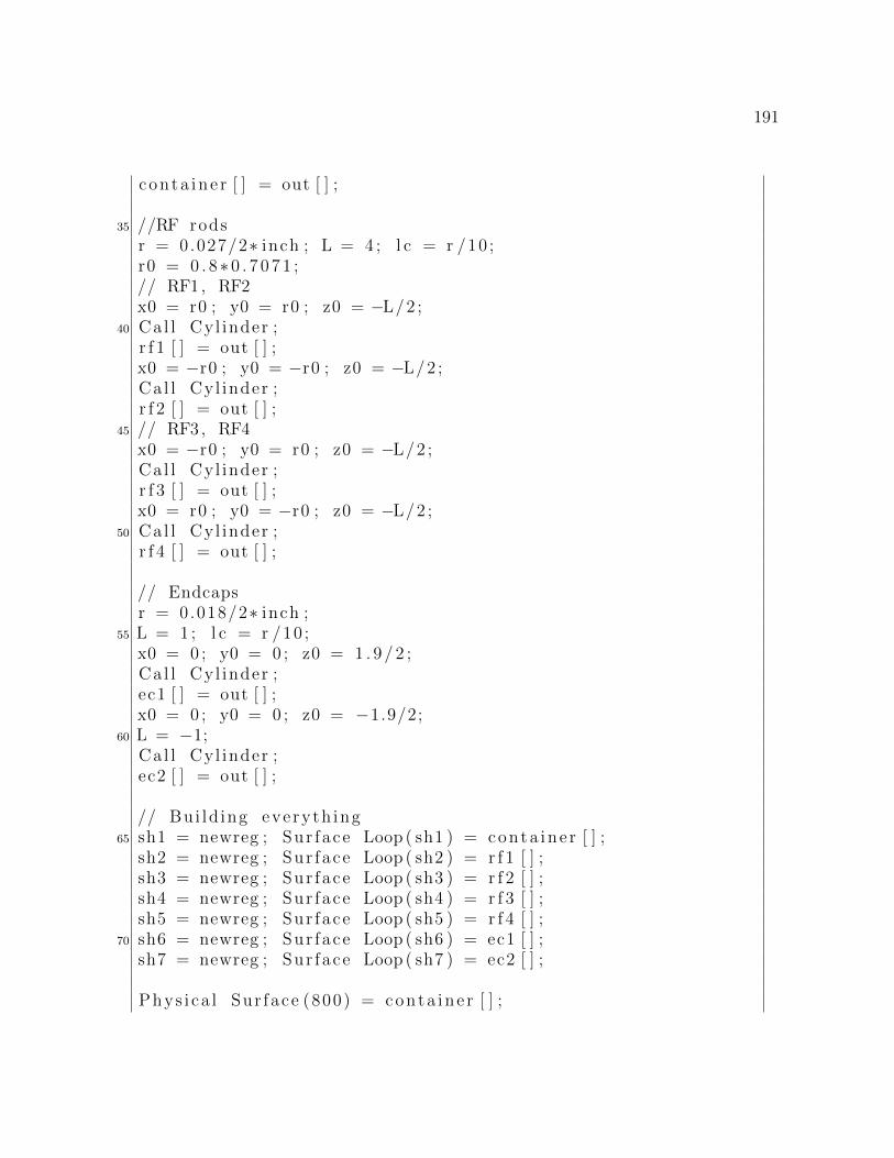
191
conta ine r [ ] = out [ ] ;
35 //RF rodsr = 0.027/2 inch ; L = 4 ; l c = r /10 ;r0 = 0 . 80 . 7 0 71 ;// RF1 , RF2x0 = r0 ; y0 = r0 ; z0 = L/2 ;
40 Cal l Cyl inder ;r f 1 [ ] = out [ ] ;x0 = r0 ; y0 = r0 ; z0 = L/2 ;Ca l l Cyl inder ;r f 2 [ ] = out [ ] ;
45 // RF3, RF4x0 = r0 ; y0 = r0 ; z0 = L/2 ;Ca l l Cyl inder ;r f 3 [ ] = out [ ] ;x0 = r0 ; y0 = r0 ; z0 = L/2 ;
50 Cal l Cyl inder ;r f 4 [ ] = out [ ] ;
// Endcapsr = 0.018/2 inch ;
55 L = 1 ; l c = r /10 ;x0 = 0 ; y0 = 0 ; z0 = 1 . 9 / 2 ;Ca l l Cyl inder ;ec1 [ ] = out [ ] ;x0 = 0 ; y0 = 0 ; z0 = 1.9/2;
60 L = 1;Ca l l Cyl inder ;ec2 [ ] = out [ ] ;
// Bui ld ing everyth ing65 sh1 = newreg ; Sur face Loop ( sh1 ) = conta ine r [ ] ;
sh2 = newreg ; Sur face Loop ( sh2 ) = r f 1 [ ] ;sh3 = newreg ; Sur face Loop ( sh3 ) = r f 2 [ ] ;sh4 = newreg ; Sur face Loop ( sh4 ) = r f 3 [ ] ;sh5 = newreg ; Sur face Loop ( sh5 ) = r f 4 [ ] ;
70 sh6 = newreg ; Sur face Loop ( sh6 ) = ec1 [ ] ;sh7 = newreg ; Sur face Loop ( sh7 ) = ec2 [ ] ;
Phys i ca l Sur face (800) = conta ine r [ ] ;

192
Phys i ca l Sur face (801) = r f 1 [ ] , r f 2 [ ] ;75 Phys i ca l Sur face (802) = r f 3 [ ] , r f 4 [ ] ;
Phys i ca l Sur face (803) = ec1 [ ] , ec2 [ ] ;
Volume (900) = sh1 , sh2 , sh3 , sh4 , sh5 , sh6 , sh7 ;Phys i ca l Volume (900) = 900 ;
See Sections 2.2 and 3.1 for the result.
B.2. SiO+ trap
Trap Geometry
1 Mesh . VolumeEdges = 0 ;
Macro yC i r c l ep0 = newp ; Point ( p0 ) = x0 , y0 , z0 ;
5 p1 = newp ; Point ( p1 ) = x0+r , y0 , z0 ;p2 = newp ; Point ( p2 ) = x0 , y0+r , z0 ;p3 = newp ; Point ( p3 ) = x0r , y0 , z0 ;p4 = newp ; Point ( p4 ) = x0 , y0r , z0 ;Cha r a c t e r i s t i c Length p1 , p2 , p3 , p4 = l c ;
10 c1 = newreg ; C i r c l e ( c1 ) = p1 , p0 , p2 ;c2 = newreg ; C i r c l e ( c2 ) = p2 , p0 , p3 ;c3 = newreg ; C i r c l e ( c3 ) = p3 , p0 , p4 ;c4 = newreg ; C i r c l e ( c4 ) = p4 , p0 , p1 ;l l = newreg ; Line Loop ( l l ) = c1 , c2 , c3 , c4 ;
15 Return
Macro Cyl inderCa l l yC i r c l e ;s1 = newreg ; Plane Sur face ( s1 ) = l l ;
20 out [ ] = Extrude 0 , 0 , L Sur face s1 ; ;De lete Volumeout [ 1 ] ; out [ 1 ] = out [ 0 ] ; out [ 0 ] = s1 ;
Return
25
// ground can

193
x0 = 0 ; y0 = 0 ; z0 = 60;r = 25 ; L = 120 ; l c = 2 ;Ca l l Cyl inder ;
30 con ta ine r [ ] = out [ ] ;
// RF rodsr = 3 . 4 3 ; L = 101 . 6 ; l c = 0 . 5 ;// RF1 , RF2
35 x0 = 4 . 5 4 ; y0 = 4 . 5 4 ; z0 = L/2 ;Ca l l Cyl inder ;r f 1 [ ] = out [ ] ;x0 = 4.54; y0 = 4.54; z0 = L/2 ;Ca l l Cyl inder ;
40 r f 2 [ ] = out [ ] ;// RF3 , RF4x0 = 4.54; y0 = 4 . 5 4 ; z0 = L/2 ;Ca l l Cyl inder ;r f 3 [ ] = out [ ] ;
45 x0 = 4 . 5 4 ; y0 = 4.54; z0 = L/2 ;Ca l l Cyl inder ;r f 4 [ ] = out [ ] ;
// End cap p l a t e 150 x0 = 0 ; y0 = 0 ; z0 = 14.6; l c = 2 ;
p1 = newp ; Point ( p1 ) = 11 .4 , 11 . 4 , z0 ;p2 = newp ; Point ( p2 ) = 11.4 , 11 . 4 , z0 ;p3 = newp ; Point ( p3 ) = 11.4 , 11.4 , z0 ;p4 = newp ; Point ( p4 ) = 11 .4 , 11.4 , z0 ;
55 Cha r a c t e r i s t i c Length p1 , p2 , p3 , p4 = l c ;l 1 = newl ; Line ( l 1 ) = p1 , p2 ;l 2 = newl ; Line ( l 2 ) = p2 , p3 ;l 3 = newl ; Line ( l 3 ) = p3 , p4 ;l 4 = newl ; Line ( l 4 ) = p4 , p1 ;
60 l l 0 = newreg ; Line Loop ( l l 0 ) = l1 , l2 , l3 , l 4 ;
r = 3 . 8 ; l c = 0 . 5 ;x0 = 4 . 5 4 ; y0 = 4 . 5 4 ;Ca l l yC i r c l e ;
65 l l 1 = l l ;x0 = 4 . 5 4 ; y0 = 4.54;Ca l l yC i r c l e ;

194
l l 2 = l l ;x0 = 4.54; y0 = 4.54;
70 Cal l yC i r c l e ;l l 3 = l l ;x0 = 4.54; y0 = 4 . 5 4 ;Ca l l yC i r c l e ;l l 4 = l l ;
75 r = 1 . 2 7 ;x0 = 0 ; y0 = 0 ;Ca l l yC i r c l e ;l l 5 = l l ;s1 = newreg ; Plane Sur face ( s1 ) = l l 0 , l l 1 , l l 2 , l l 3 , l l 4 ,
,! l l 5 ;80 out [ ] = Extrude 0 , 0 , 2.5 Sur face s1 ; ;
De lete Volumeout [ 1 ] ; out [ 1 ] = out [ 0 ] ; out [ 0 ] = s1 ;ec11 [ ] = out [ ] ;
85 // End cap tube 1x0 = 0 ; y0 = 0 ; z0 += 0 . 1 ; l c = 0 . 5 ;r = 1 . 2 7 ;Ca l l yC i r c l e ;l l 6 = l l ;
90 r = 2 . 0 8 ;Ca l l yC i r c l e ;l l 7 = l l ;s1 = newreg ; Plane Sur face ( s1 ) = l l 7 , l l 6 ;out [ ] = Extrude 0 , 0 , 4.40.1 Sur face s1 ; ;
95 Delete Volumeout [ 1 ] ; out [ 1 ] = out [ 0 ] ; out [ 0 ] = s1 ;ec12 [ ] = out [ ] ;
100 // End cap p l a t e 2x0 = 0 ; y0 = 0 ; z0 = 14 . 6 ; l c = 2 ;p1 = newp ; Point ( p1 ) = 11 .4 , 11 . 4 , z0 ;p2 = newp ; Point ( p2 ) = 11.4 , 11 . 4 , z0 ;p3 = newp ; Point ( p3 ) = 11.4 , 11.4 , z0 ;
105 p4 = newp ; Point ( p4 ) = 11 .4 , 11.4 , z0 ;Cha r a c t e r i s t i c Length p1 , p2 , p3 , p4 = l c ;l 1 = newl ; Line ( l 1 ) = p1 , p2 ;
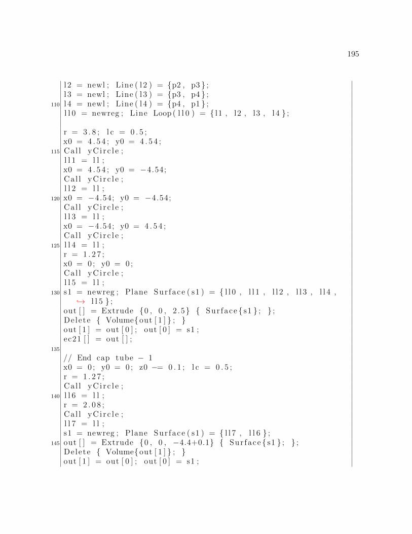
195
l 2 = newl ; Line ( l 2 ) = p2 , p3 ;l 3 = newl ; Line ( l 3 ) = p3 , p4 ;
110 l 4 = newl ; Line ( l 4 ) = p4 , p1 ;l l 0 = newreg ; Line Loop ( l l 0 ) = l1 , l2 , l3 , l 4 ;
r = 3 . 8 ; l c = 0 . 5 ;x0 = 4 . 5 4 ; y0 = 4 . 5 4 ;
115 Cal l yC i r c l e ;l l 1 = l l ;x0 = 4 . 5 4 ; y0 = 4.54;Ca l l yC i r c l e ;l l 2 = l l ;
120 x0 = 4.54; y0 = 4.54;Ca l l yC i r c l e ;l l 3 = l l ;x0 = 4.54; y0 = 4 . 5 4 ;Ca l l yC i r c l e ;
125 l l 4 = l l ;r = 1 . 2 7 ;x0 = 0 ; y0 = 0 ;Ca l l yC i r c l e ;l l 5 = l l ;
130 s1 = newreg ; Plane Sur face ( s1 ) = l l 0 , l l 1 , l l 2 , l l 3 , l l 4 ,,! l l 5 ;
out [ ] = Extrude 0 , 0 , 2 .5 Sur face s1 ; ;De lete Volumeout [ 1 ] ; out [ 1 ] = out [ 0 ] ; out [ 0 ] = s1 ;ec21 [ ] = out [ ] ;
135
// End cap tube 1x0 = 0 ; y0 = 0 ; z0 = 0 . 1 ; l c = 0 . 5 ;r = 1 . 2 7 ;Ca l l yC i r c l e ;
140 l l 6 = l l ;r = 2 . 0 8 ;Ca l l yC i r c l e ;l l 7 = l l ;s1 = newreg ; Plane Sur face ( s1 ) = l l 7 , l l 6 ;
145 out [ ] = Extrude 0 , 0 , 4.4+0.1 Sur face s1 ; ;De lete Volumeout [ 1 ] ; out [ 1 ] = out [ 0 ] ; out [ 0 ] = s1 ;

196
ec22 [ ] = out [ ] ;
150
// bu i ld everyth ingsh1 = newreg ; Sur face Loop ( sh1 ) = conta ine r [ ] ;sh2 = newreg ; Sur face Loop ( sh2 ) = r f 1 [ ] ;sh3 = newreg ; Sur face Loop ( sh3 ) = r f 2 [ ] ;
155 sh4 = newreg ; Sur face Loop ( sh4 ) = r f 3 [ ] ;sh5 = newreg ; Sur face Loop ( sh5 ) = r f 4 [ ] ;sh6 = newreg ; Sur face Loop ( sh6 ) = ec11 [ ] ;sh7 = newreg ; Sur face Loop ( sh7 ) = ec12 [ ] ;sh8 = newreg ; Sur face Loop ( sh8 ) = ec21 [ ] ;
160 sh9 = newreg ; Sur face Loop ( sh9 ) = ec22 [ ] ;
Phys i ca l Sur face (800) = conta ine r [ ] ;Phys i ca l Sur face (801) = r f 1 [ ] , r f 2 [ ] ;
165 Phys i ca l Sur face (802) = r f 3 [ ] , r f 4 [ ] ;Phys i ca l Sur face (803) = ec11 [ ] , ec12 [ ] ;Phys i ca l Sur face (804) = ec21 [ ] , ec22 [ ] ;
170 Volume (900) = sh1 , sh2 , sh3 , sh4 , sh5 , sh6 , sh7 , sh8 , sh9 ;Phys i ca l Volume (900) = 900 ;

197
Table B.1. Fitting region (x, y, z) | px2 + y2 < 1.5, |z| < 5
l m RF-1 RF-2 Endcap
0 0 4.92 101 4.92 101 1.59 102
2 0 2.00 103 2.18 103 3.97 103
2 2 1.12 104 7.65 105 3.28 105
2 -2 4.50 101 4.50 101 1.61 104
4 0 6.51 105 4.62 105 1.47 104
4 2 5.12 106 3.15 106 1.34 106
4 -2 2.02 104 2.89 104 1.32 104
4 4 1.13 106 3.74 107 4.19 107
4 -4 1.65 102 4.56 102 5.96 103
6 0 2.49 106 3.25 106 3.84 106
6 2 1.17 107 5.61 108 2.45 108
6 -2 2.97 105 2.89 105 2.06 105
6 4 3.17 109 7.82 1010 5.50 1010
6 -4 1.03 102 5.97 103 2.04 103
6 6 4.61 109 6.11 109 1.39 109
6 -6 1.65 1.20 8.79 102
8 0 2.02 108 3.35 108 2.38 108
8 2 1.14 109 4.08 1010 1.74 1010
8 -2 2.91 106 3.04 106 1.03 106
8 4 9.61 1012 1.84 1011 9.08 1012
8 -4 3.35 104 3.29 104 6.98 105
8 6 2.30 1013 7.19 1013 3.11 1012
8 -6 3.78 101 2.70 101 3.58 102
8 8 1.09 1011 6.40 1012 3.04 1013
8 -8 1.75 102 3.37 102 3.25 101

198
B.3. AlH+ trap
Trap Geometry
1 Mesh . VolumeEdges = 0 ;
Macro yC i r c l ep0 = newp ; Point ( p0 ) = x0 , y0 , z0 ;
5 p1 = newp ; Point ( p1 ) = x0+r , y0 , z0 ;p2 = newp ; Point ( p2 ) = x0 , y0+r , z0 ;p3 = newp ; Point ( p3 ) = x0r , y0 , z0 ;p4 = newp ; Point ( p4 ) = x0 , y0r , z0 ;Cha r a c t e r i s t i c Length p1 , p2 , p3 , p4 = l c ;
10 c1 = newreg ; C i r c l e ( c1 ) = p1 , p0 , p2 ;c2 = newreg ; C i r c l e ( c2 ) = p2 , p0 , p3 ;c3 = newreg ; C i r c l e ( c3 ) = p3 , p0 , p4 ;c4 = newreg ; C i r c l e ( c4 ) = p4 , p0 , p1 ;l l = newreg ; Line Loop ( l l ) = c1 , c2 , c3 , c4 ;
15 Return
Macro Cyl inderCa l l yC i r c l e ;s1 = newreg ; Plane Sur face ( s1 ) = l l ;
20 out [ ] = Extrude 0 , 0 , L Sur face s1 ; ;De lete Volumeout [ 1 ] ; out [ 1 ] = out [ 0 ] ; out [ 0 ] = s1 ;
Return
25
// ground canx0 = 0 ; y0 = 0 ; z0 = 40;r = 20 ; L = 70 ; l c = 2 ;Ca l l Cyl inder ;
30 con ta ine r [ ] = out [ ] ;
// RF rodsr = 3 . 4 3 ; L = 51.6; l c = 0 . 5 ; z0 = 17 . 1 ;// RF1 , RF2
35 x0 = 4 . 5 4 ; y0 = 4 . 5 4 ;Ca l l Cyl inder ;
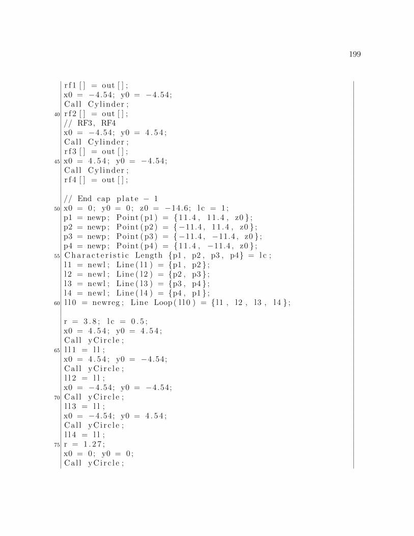
199
r f 1 [ ] = out [ ] ;x0 = 4.54; y0 = 4.54;Ca l l Cyl inder ;
40 r f 2 [ ] = out [ ] ;// RF3 , RF4x0 = 4.54; y0 = 4 . 5 4 ;Ca l l Cyl inder ;r f 3 [ ] = out [ ] ;
45 x0 = 4 . 5 4 ; y0 = 4.54;Ca l l Cyl inder ;r f 4 [ ] = out [ ] ;
// End cap p l a t e 150 x0 = 0 ; y0 = 0 ; z0 = 14.6; l c = 1 ;
p1 = newp ; Point ( p1 ) = 11 .4 , 11 . 4 , z0 ;p2 = newp ; Point ( p2 ) = 11.4 , 11 . 4 , z0 ;p3 = newp ; Point ( p3 ) = 11.4 , 11.4 , z0 ;p4 = newp ; Point ( p4 ) = 11 .4 , 11.4 , z0 ;
55 Cha r a c t e r i s t i c Length p1 , p2 , p3 , p4 = l c ;l 1 = newl ; Line ( l 1 ) = p1 , p2 ;l 2 = newl ; Line ( l 2 ) = p2 , p3 ;l 3 = newl ; Line ( l 3 ) = p3 , p4 ;l 4 = newl ; Line ( l 4 ) = p4 , p1 ;
60 l l 0 = newreg ; Line Loop ( l l 0 ) = l1 , l2 , l3 , l 4 ;
r = 3 . 8 ; l c = 0 . 5 ;x0 = 4 . 5 4 ; y0 = 4 . 5 4 ;Ca l l yC i r c l e ;
65 l l 1 = l l ;x0 = 4 . 5 4 ; y0 = 4.54;Ca l l yC i r c l e ;l l 2 = l l ;x0 = 4.54; y0 = 4.54;
70 Cal l yC i r c l e ;l l 3 = l l ;x0 = 4.54; y0 = 4 . 5 4 ;Ca l l yC i r c l e ;l l 4 = l l ;
75 r = 1 . 2 7 ;x0 = 0 ; y0 = 0 ;Ca l l yC i r c l e ;

200
l l 5 = l l ;s1 = newreg ; Plane Sur face ( s1 ) = l l 0 , l l 1 , l l 2 , l l 3 , l l 4 ,
,! l l 5 ;80 out [ ] = Extrude 0 , 0 , 2.5 Sur face s1 ; ;
De lete Volumeout [ 1 ] ; out [ 1 ] = out [ 0 ] ; out [ 0 ] = s1 ;ec1 [ ] = out [ ] ;
85 // End cap p l a t e 2x0 = 0 ; y0 = 0 ; z0 = 14 . 6 ; l c = 1 ;p1 = newp ; Point ( p1 ) = 11 .4 , 11 . 4 , z0 ;p2 = newp ; Point ( p2 ) = 11.4 , 11 . 4 , z0 ;p3 = newp ; Point ( p3 ) = 11.4 , 11.4 , z0 ;
90 p4 = newp ; Point ( p4 ) = 11 .4 , 11.4 , z0 ;Cha r a c t e r i s t i c Length p1 , p2 , p3 , p4 = l c ;l 1 = newl ; Line ( l 1 ) = p1 , p2 ;l 2 = newl ; Line ( l 2 ) = p2 , p3 ;l 3 = newl ; Line ( l 3 ) = p3 , p4 ;
95 l 4 = newl ; Line ( l 4 ) = p4 , p1 ;l l 0 = newreg ; Line Loop ( l l 0 ) = l1 , l2 , l3 , l 4 ;
r = 3 . 8 ; l c = 0 . 5 ;x0 = 4 . 5 4 ; y0 = 4 . 5 4 ;
100 Cal l yC i r c l e ;l l 1 = l l ;x0 = 4 . 5 4 ; y0 = 4.54;Ca l l yC i r c l e ;l l 2 = l l ;
105 x0 = 4.54; y0 = 4.54;Ca l l yC i r c l e ;l l 3 = l l ;x0 = 4.54; y0 = 4 . 5 4 ;Ca l l yC i r c l e ;
110 l l 4 = l l ;r = 1 . 2 7 ;x0 = 0 ; y0 = 0 ;Ca l l yC i r c l e ;l l 5 = l l ;
115 s1 = newreg ; Plane Sur face ( s1 ) = l l 0 , l l 1 , l l 2 , l l 3 , l l 4 ,,! l l 5 ;
out [ ] = Extrude 0 , 0 , 2 .5 Sur face s1 ; ;

201
Delete Volumeout [ 1 ] ; out [ 1 ] = out [ 0 ] ; out [ 0 ] = s1 ;ec2 [ ] = out [ ] ;
120
// bu i ld everyth ingsh1 = newreg ; Sur face Loop ( sh1 ) = conta ine r [ ] ;
125 sh2 = newreg ; Sur face Loop ( sh2 ) = r f 1 [ ] ;sh3 = newreg ; Sur face Loop ( sh3 ) = r f 2 [ ] ;sh4 = newreg ; Sur face Loop ( sh4 ) = r f 3 [ ] ;sh5 = newreg ; Sur face Loop ( sh5 ) = r f 4 [ ] ;sh6 = newreg ; Sur face Loop ( sh6 ) = ec1 [ ] ;
130 sh7 = newreg ; Sur face Loop ( sh7 ) = ec2 [ ] ;
Phys i ca l Sur face (800) = conta ine r [ ] ;Phys i ca l Sur face (801) = r f 1 [ ] , r f 2 [ ] ;
135 Phys i ca l Sur face (802) = r f 3 [ ] , r f 4 [ ] ;Phys i ca l Sur face (803) = ec1 [ ] , ec2 [ ] ;
Volume (900) = sh1 , sh2 , sh3 , sh4 , sh5 , sh6 , sh7 ;Phys i ca l Volume (900) = 900 ;
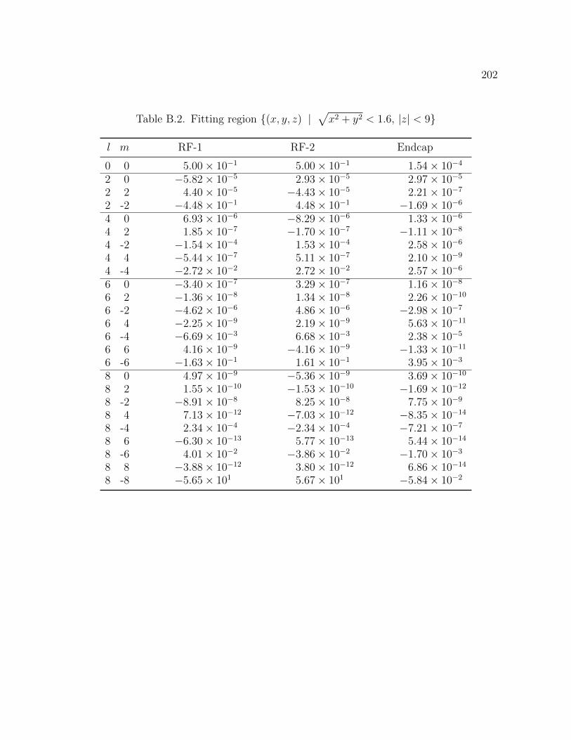
202
Table B.2. Fitting region (x, y, z) | px2 + y2 < 1.6, |z| < 9
l m RF-1 RF-2 Endcap
0 0 5.00 101 5.00 101 1.54 104
2 0 5.82 105 2.93 105 2.97 105
2 2 4.40 105 4.43 105 2.21 107
2 -2 4.48 101 4.48 101 1.69 106
4 0 6.93 106 8.29 106 1.33 106
4 2 1.85 107 1.70 107 1.11 108
4 -2 1.54 104 1.53 104 2.58 106
4 4 5.44 107 5.11 107 2.10 109
4 -4 2.72 102 2.72 102 2.57 106
6 0 3.40 107 3.29 107 1.16 108
6 2 1.36 108 1.34 108 2.26 1010
6 -2 4.62 106 4.86 106 2.98 107
6 4 2.25 109 2.19 109 5.63 1011
6 -4 6.69 103 6.68 103 2.38 105
6 6 4.16 109 4.16 109 1.33 1011
6 -6 1.63 101 1.61 101 3.95 103
8 0 4.97 109 5.36 109 3.69 1010
8 2 1.55 1010 1.53 1010 1.69 1012
8 -2 8.91 108 8.25 108 7.75 109
8 4 7.13 1012 7.03 1012 8.35 1014
8 -4 2.34 104 2.34 104 7.21 107
8 6 6.30 1013 5.77 1013 5.44 1014
8 -6 4.01 102 3.86 102 1.70 103
8 8 3.88 1012 3.80 1012 6.86 1014
8 -8 5.65 101 5.67 101 5.84 102

203
APPENDIX C
Drawings

204
Figure C.1. Macro stand for RF electrodes - sheet 1
Units: inches/degree. Tolerance: ±0.005”. Material: Macro

205
Figure C.2. Macro stand - sheet 2

206
Figure C.3. Macro stand for endcap electrodes
Units: inches/degree. Tolerance: ±0.005”. Material: Macro

207
Figure C.4. Trap base plate
Units: inches/degree. Tolerance: ±0.01”. Material: stainless steel 316

208
Figure C.5. Single ion trap assembly - sheet 1

209
Figure C.6. Single ion trap assembly - sheet 2

210
Figure C.7. Single ion trap assembly - sheet 3
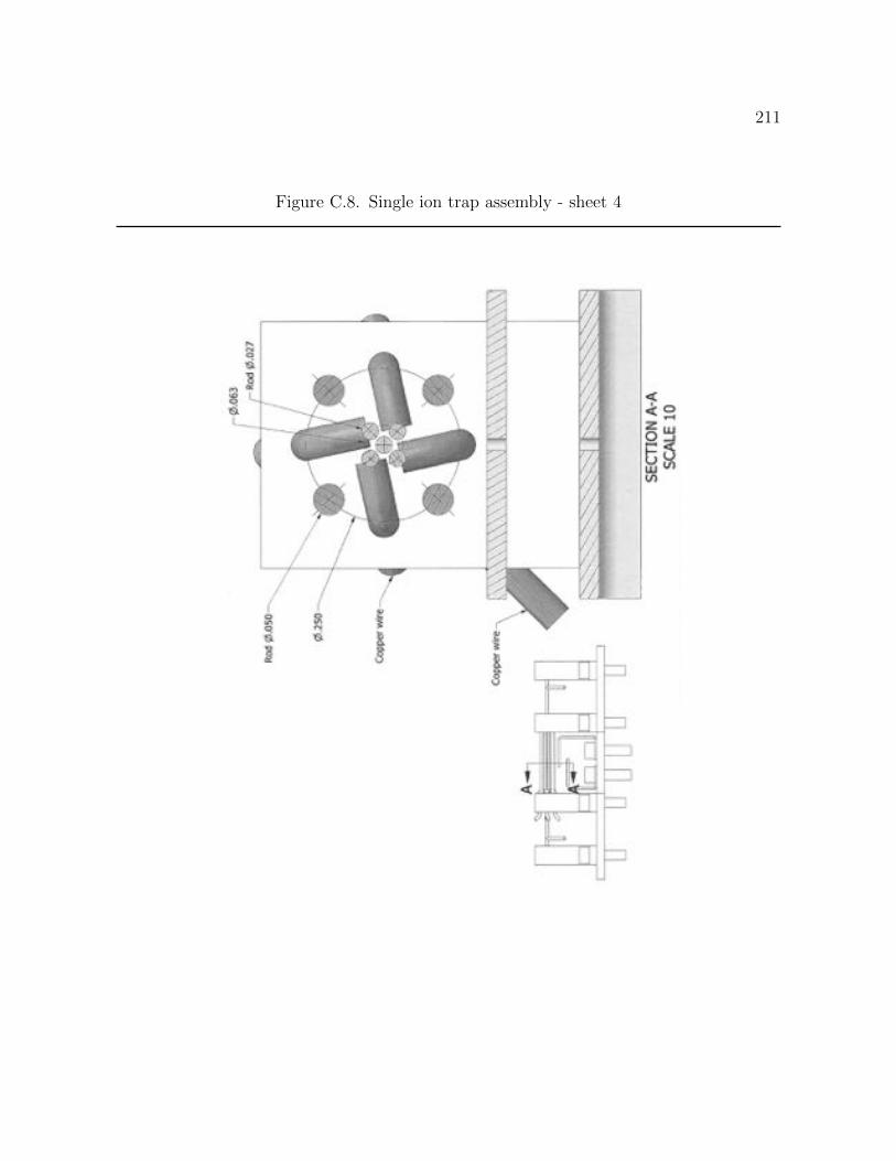
211
Figure C.8. Single ion trap assembly - sheet 4

212
Figure C.9. Trap stand
Units: inches/degree. Tolerance: ±0.01”. Material: stainless steel 316

213
Figure C.10. 6CF flange
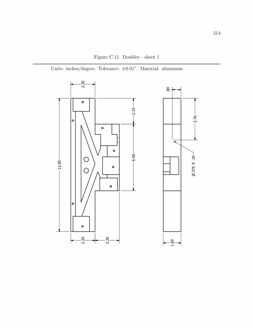
214
Figure C.11. Doubler - sheet 1
Units: inches/degree. Tolerance: ±0.01”. Material: aluminum
PR
OD
UC
ED B
Y AN
AU
TOD
ESK
ED
UC
ATIO
NA
L PR
OD
UC
T
PR
OD
UC
ED B
Y AN
AU
TOD
ESK
ED
UC
ATIO
NA
L PR
OD
UC
T
PRODUCED BY AN AUTODESK EDUCATIONAL PRODUCTPRODUCED BY AN AUTODESK EDUCATIONAL PRODUCT
doub
ler
Qua
ntity
:M
ater
ial:
Uni
ts:
inch
es/d
egre
eTo
lera
nces
:
File
nam
e: p
latf
orm
.ipt
Dat
e:
Yen-
Wei
Lin
610-
4011
500-
6003
3743
Tech
FB3
1 /
7-19
591 al
umin
um
y-lin
@u.
nort
hwes
tern
.edu
Pa
ge:
1 /
4
+/-
0.01
12.0
0
2.20
2.20
2.20
2.33
6.00
1.60
3.76
.80
P.3
75 Z
.20

215
Figure C.12. Doubler - sheet 2
Units: inches/degree. Tolerance: ±0.01”. Material: aluminum
PR
OD
UC
ED B
Y AN
AU
TOD
ESK
ED
UC
ATIO
NA
L PR
OD
UC
T
PR
OD
UC
ED B
Y AN
AU
TOD
ESK
ED
UC
ATIO
NA
L PR
OD
UC
T
PRODUCED BY AN AUTODESK EDUCATIONAL PRODUCTPRODUCED BY AN AUTODESK EDUCATIONAL PRODUCT
Qua
ntity
:M
ater
ial:
Uni
ts:
inch
es/d
egre
eTo
lera
nces
:
File
nam
e: p
latf
orm
.ipt
Dat
e:
Te
ch F
B31
/ 7-
1959
Pa
ge:
2 /
4
1.38
1.50.20
1.19
1.50.20
1.50
.50
1.50
1.00
.92
1.60
1.16
1.47
1.54
1.60
.42
1.40
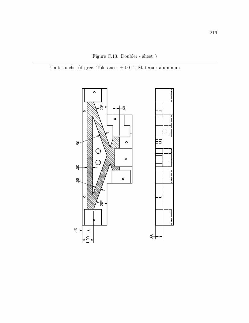
216
Figure C.13. Doubler - sheet 3
Units: inches/degree. Tolerance: ±0.01”. Material: aluminum
PR
OD
UC
ED B
Y AN
AU
TOD
ESK
ED
UC
ATIO
NA
L PR
OD
UC
T
PR
OD
UC
ED B
Y AN
AU
TOD
ESK
ED
UC
ATIO
NA
L PR
OD
UC
T
PRODUCED BY AN AUTODESK EDUCATIONAL PRODUCT
PRODUCED BY AN AUTODESK EDUCATIONAL PRODUCT
Qua
ntity
:M
ater
ial:
Uni
ts:
inch
es/d
egre
eTo
lera
nces
:
File
nam
e: p
latf
orm
.ipt
Dat
e:
Te
ch F
B31
/ 7-
1959
Pa
ge:
3 /
4
.50
.50
.50
.60
.43
1.00
20°
20°
.60

217
Figure C.14. Doubler - sheet 4
Units: inches/degree. Tolerance: ±0.01”. Material: aluminum
PR
OD
UC
ED B
Y AN
AU
TOD
ESK
ED
UC
ATIO
NA
L PR
OD
UC
T
PR
OD
UC
ED B
Y AN
AU
TOD
ESK
ED
UC
ATIO
NA
L PR
OD
UC
T
PRODUCED BY AN AUTODESK EDUCATIONAL PRODUCT
PRODUCED BY AN AUTODESK EDUCATIONAL PRODUCT
Qua
ntity
:M
ater
ial:
Uni
ts:
inch
es/d
egre
eTo
lera
nces
:
File
nam
e: p
latf
orm
.ipt
Dat
e:
Te
ch F
B31
/ 7-
1959
Pa
ge:
4 /
4
A2A1
A3
A4A5
B2B3
B1
C1C3
HO
LE T
ABLE
HO
LEXD
IMYD
IMD
ESCR
IPTI
ON
A12.
14-1
.63
8-32
UN
C -
2BA2
.40
-1.4
28-
32 U
NC
- 2B
A35.
65-.
668-
32 U
NC
- 2B
A47.
991.
118-
32 U
NC
- 2B
A5-3
.20
1.14
8-32
UN
C -
2BB1
3.60
-1.7
08-
32 U
NC
- 2B
Z .5
0B3
-1.1
72.
008-
32 U
NC
- 2B
Z .5
0B2
6.33
2.00
8-32
UN
C -
2B Z
.50
C11.
83.7
9P
.27
THRU
X P
.44 Z
1.4
0
C32.
83.7
9P
.27
THRU
X P
.44 Z
1.4
0

218
Figure C.15. Cover for the doubler
Units: inches/degree. Tolerance: ±0.01”. Material: aluminum
PR
OD
UC
ED B
Y AN
AU
TOD
ESK
ED
UC
ATIO
NA
L PR
OD
UC
T
PR
OD
UC
ED B
Y AN
AU
TOD
ESK
ED
UC
ATIO
NA
L PR
OD
UC
T
PRODUCED BY AN AUTODESK EDUCATIONAL PRODUCTPRODUCED BY AN AUTODESK EDUCATIONAL PRODUCT
cove
r
Qua
ntity
:M
ater
ial:
Uni
ts:
inch
es/d
egre
eTo
lera
nces
:
File
nam
e: li
d.ip
t
Dat
e:
Yen-
Wei
Lin
610-
4011
500-
6003
3743
Tech
FB3
1 /
7-19
591 al
umin
um
y-lin
@u.
nort
hwes
tern
.edu
Pa
ge:
1 /
1
+/-
0.01
12.0
0
2.20
2.20
2.20
6.00
2.33
A1A2
A3 HO
LE T
ABLE
HO
LEXD
IMYD
IMD
ESCR
IPTI
ON
A1-1
.17
2.00
P.1
8 TH
RUA2
6.33
2.00
P.1
8 TH
RUA3
3.60
-1.7
0P
.18
THRU
plat
e th
ickn
ess:
1/8

219
Figure C.16. Crystal holder
Units: inches/degree. Tolerance: ±0.01”. Material: aluminum
PRODUCED BY AN AUTODESK EDUCATIONAL PRODUCT
PRODUCED BY AN AUTODESK EDUCATIONAL PRODUCT
PR
OD
UC
ED B
Y AN
AU
TOD
ESK
ED
UC
ATIO
NA
L PR
OD
UC
T PR
OD
UC
ED BY AN
AUTO
DESK
EDU
CATIO
NA
L PRO
DU
CT
crystal holder
Quantity:Material:
Units: inches/degree Tolerances:
Filename: xtal holder.ipt
Date:
Yen-Wei Lin
610-4011500-60033743Tech FB31 / 7-1959
1aluminum
Page: 1 / 1
+/-0.01
P.50
.25
.30 .10
.20.35
.10
.15
8-32 UNC - 2B