
Towards the assessment of a residential electric storage ...
134
Towards the assessment of a residential electric storage system: analysis of Canadian residential electricity use and the development of a lithium-ion battery model by Neil Saldanha, B.Sc., Mechanical Engineering Queen’s University A thesis submitted to the Faculty of Graduate and Postdoctoral Affairs in partial fulfillment of the requirements for the degree of Master of Applied Science in Mechanical Engineering Ottawa-Carleton Institute for Mechanical and Aerospace Engineering Department of Mechanical and Aerospace Engineering Carleton University Ottawa, Ontario August, 2010 c Copyright Neil Saldanha, 2010
Transcript of Towards the assessment of a residential electric storage ...
Towards the assessment of a residential electricstorage system: analysis of Canadian residential
electricity use and the development of alithium-ion battery model
by
Neil Saldanha, B.Sc., Mechanical Engineering
Queen’s University
A thesis submitted to the
Faculty of Graduate and Postdoctoral Affairs
in partial fulfillment of the requirements for the degree of
Master of Applied Science in Mechanical Engineering
Ottawa-Carleton Institute for Mechanical and Aerospace Engineering
Department of Mechanical and Aerospace Engineering
Carleton University
Ottawa, Ontario
August, 2010
c©Copyright
Neil Saldanha, 2010

The undersigned hereby recommends to the
Faculty of Graduate and Postdoctoral Affairs
acceptance of the thesis
Towards the assessment of a residential electric storagesystem: analysis of Canadian residential electricity use and
the development of a lithium-ion battery model
submitted by Neil Saldanha, B.Sc., Mechanical Engineering
Queen’s University
in partial fulfillment of the requirements for the degree of
Master of Applied Science in Mechanical Engineering
ii

Professor Ian Beausoleil-Morrison, Thesis Supervisor
Professor Cynthia Cruickshank
Professor Steven McGarry
Professor Atef Fahim
Dr. Ken Darcovich
Professor Metin Yaras, Chair,Department of Mechanical and Aerospace Engineering
Ottawa-Carleton Institute for Mechanical and Aerospace Engineering
Department of Mechanical and Aerospace Engineering
Carleton University
August, 2010
iii

Abstract
Peak electricity demand from residential houses leads to increased greenhouse gas
emissions from inefficient electricity production. The coincidental use of household
appliances and lighting, known as non-HVAC loads, and air-conditioners creates pe-
riods of increased electricity demand on utility providers in Ontario. This leads to
electricity production from fuels such as coal that produce excessive greenhouse gas
emissions.
To assess the potential of a micro-cogeneration device coupled with lithium-ion
battery electricity storage to reduce peak electricity demand using building simula-
tion, residential electricity use of Canadian houses must be accurately represented.
Thus, electricity use from twelve houses in the Ottawa, Ontario area was collected
over a one year period, beginning in the summer of 2009. The project measured
and analyzed non-HVAC and space cooling electricity use at one-minute intervals.
The daily non-HVAC electricity profiles measured in this study show more variation
and higher occurrences of peak loads compared to previously developed synthetically
generated profiles. Both non-HVAC and space cooling profiles show large variations
in electricity consumption between households. The relationship between daily space
cooling electricity consumption and outdoor temperature is shown.
A lithium-ion battery model was then developed in the building simulation pro-
gram ESP-r. The model accounts for changes in performance due to varying temper-
ature and current, and addresses long-term degradation over a battery’s life cycle.
The model was calibrated and validated using simulated data from the National
Research Council’s Institute for Chemical Process and Environmental Technology.
The functionality of the lithium-ion model simulated in a household and coupled
with a Stirling engine micro-cogeneration model is demonstrated.
Following the implementation of an optimized controller, a lithium-ion battery
simulated with a micro-cogeneration device can be sized and fully assessed. The
research in this document provides the foundation for this assessment.
iv

To my family for keeping me grounded, and my friends for keeping me up late...
v

Acknowledgments
First and foremost I would like to acknowledge my supervisor, Dr. Ian Beausoleil-
Morrison. Not only would this work had not been possible without his academic
guidance, but his personal mentorship and approach to life will be something that I
will never forget.
I would like to acknowledge Dr. Ken Darcovich, Dr. Isobel Davidson and Dr.
Eduardo Henquin at the National Research Council’s Institute for Chemical Process
and Environmental Technology. Their support and guidance helped me to branch
into a new area of science.
Special thanks also goes to Dave Kuhnle and Steve Kuhnle of Nepean Electric.
Not only did they help me in getting this project off its feet, but their expertise and
patience went beyond the call of professionalism.
Thanks as well to Dr. Guy Newsham at the National Research Council’s Institute
for Research in Construction. Their support and funding allowed the results from
this project to exceed further.
Lastly, a very special thank you to my colleagues and friends in The Sustainable
Building Energy Systems Laboratory at Carleton University. I came to this school
not knowing what to expect, but your support throughout this project made it, and
I, succeed.
vi

Table of Contents
Abstract iv
Acknowledgments vi
Table of Contents vii
List of Tables ix
List of Figures x
Nomenclature xv
1 Introduction and literature review 1
1.1 Introduction . . . . . . . . . . . . . . . . . . . . . . . . . . . . . . . . 1
1.2 Literature review . . . . . . . . . . . . . . . . . . . . . . . . . . . . . 2
1.2.1 Canadian residential energy use and the electric grid . . . . . 2
1.2.2 Micro-cogeneration . . . . . . . . . . . . . . . . . . . . . . . . 5
1.2.3 Electricity storage and lithium ion batteries . . . . . . . . . . 6
1.2.4 RES modelling . . . . . . . . . . . . . . . . . . . . . . . . . . 8
1.2.5 Residential load monitoring . . . . . . . . . . . . . . . . . . . 9
1.3 Research objectives . . . . . . . . . . . . . . . . . . . . . . . . . . . . 10
1.4 Thesis outline . . . . . . . . . . . . . . . . . . . . . . . . . . . . . . . 11
2 ESP-r simulation methods 12
2.1 The ESP-r thermal, air flow and plant networks . . . . . . . . . . . . 12
2.2 Electrical power flow network in ESP-r . . . . . . . . . . . . . . . . . 17
3 Non-HVAC and Space Cooling Electric Loads 21
3.1 Previous work and synthetically generated profiles . . . . . . . . . . . 21
vii

3.2 Electrical measurement project . . . . . . . . . . . . . . . . . . . . . 24
3.2.1 Measurement methods and data analysis . . . . . . . . . . . . 26
3.3 Non-HVAC data results . . . . . . . . . . . . . . . . . . . . . . . . . 32
3.4 Space cooling data analysis . . . . . . . . . . . . . . . . . . . . . . . . 42
4 Lithium-ion battery model 47
4.1 Lithium-ion battery chemistry . . . . . . . . . . . . . . . . . . . . . . 47
4.2 Lithium-ion battery modelling . . . . . . . . . . . . . . . . . . . . . . 53
4.3 Li-ion modelling approach for present work . . . . . . . . . . . . . . . 56
4.4 Implementation in ESP-r battery subroutine . . . . . . . . . . . . . . 59
5 Calibration of the Battery Model 65
5.1 Calibrated source data . . . . . . . . . . . . . . . . . . . . . . . . . . 65
5.2 Calibration parameters . . . . . . . . . . . . . . . . . . . . . . . . . . 67
5.2.1 Geometric parameters . . . . . . . . . . . . . . . . . . . . . . 68
5.2.2 Current and temperature parameters . . . . . . . . . . . . . . 74
6 Demonstration of new modelling capabilities 84
6.1 Li-ion battery model debugging . . . . . . . . . . . . . . . . . . . . . 84
6.2 Validation with simulated data from ICPET . . . . . . . . . . . . . . 85
6.3 Demonstration of integrated system . . . . . . . . . . . . . . . . . . . 88
6.3.1 ESP-r model description . . . . . . . . . . . . . . . . . . . . . 88
6.3.2 Simulation results . . . . . . . . . . . . . . . . . . . . . . . . . 90
7 Conclusions & Future Work 95
7.1 Conclusions . . . . . . . . . . . . . . . . . . . . . . . . . . . . . . . . 95
7.2 Future Work: Non-HVAC and space cooling . . . . . . . . . . . . . . 97
7.3 Future Work: Li-ion battery model . . . . . . . . . . . . . . . . . . . 100
List of References 105
Appendix A Example of calibration data provided from NRC-ICPET
(0.01 A ·m−2 and 25oC) 112
Appendix B Calibration parameters for the Li-ion battery model 114
viii

List of Tables
3.1 Annual electric consumption of the participating households in kWh ·yr−1. Note that bias exists due to the lack of a complete year of
collected data. . . . . . . . . . . . . . . . . . . . . . . . . . . . . . . 25
3.2 Watt-hours per pulse resolution in logging equipment in the measure-
ment project. . . . . . . . . . . . . . . . . . . . . . . . . . . . . . . . 27
3.3 Bias errors of measuring devices. . . . . . . . . . . . . . . . . . . . . 28
3.4 95th percentile non-HVAC electrical power draw of the households in
the measurement project sorted by annual energy consumption level
at one minute intervals. . . . . . . . . . . . . . . . . . . . . . . . . . . 34
3.5 95th percentile non-HVAC electrical power draw of the synthetically
generated profiles sorted by annual energy consumption level. . . . . 34
5.1 List of data sets provided by NRC-ICPET. 16 data sets of discharge
curves were provided, each one at either constant current or constant
temperature. . . . . . . . . . . . . . . . . . . . . . . . . . . . . . . . . 66
5.2 Internal resistance coefficients used for the model calibration. . . . . 78
5.3 Internal resistance coefficients used for model calibration. . . . . . . 80
5.4 ∆V (T ) values to calibrate li-ion battery model. . . . . . . . . . . . . 83
6.1 Current and temperature statistics for annual simulation. . . . . . . 92
ix

List of Figures
1.1 Simulation of electricity used for space cooling in a typical Canadian
dwelling in Ottawa, Ontario on June 7th, 2008. . . . . . . . . . . . . 3
1.2 Market electricity demand and supply by generation source in Ontario
on June 7th, 2008. Note: “Other” indicates gas fired and wood waste
sources. . . . . . . . . . . . . . . . . . . . . . . . . . . . . . . . . . . 4
1.3 Schematic of lithium ion battery. . . . . . . . . . . . . . . . . . . . . 7
1.4 Schematic of Li-ion micro-cogeneration model. . . . . . . . . . . . . . 9
2.1 Energy flow paths and energy generation at an air point node in ESP-r. 14
2.2 Energy flow paths and energy generation at construction nodes in ESP-r. 14
2.3 Schematic of example HVAC system in ESP-r. . . . . . . . . . . . . 16
2.4 Matrix equations for thermal domain at ith node with plant injection. 18
2.5 Example of electrical network schematic in ESP-r. . . . . . . . . . . 19
3.1 Comparison of typical electricity profile taken at one minute intervals
and averaged over one hour intervals. . . . . . . . . . . . . . . . . . 23
3.2 Measuring devices installed at the electric panel of a participant in the
electric measurement project. . . . . . . . . . . . . . . . . . . . . . . 25
3.3 Bias error as a function of average power drawn by the entire household
over one minute. Note that this is for a 240 V circuit with a 50 A CT
attached, and is assumed to be working within an acceptable current
range and with a phase angle of zero. . . . . . . . . . . . . . . . . . . 29
3.4 95th percentile illustration from a cumulative histogram from the data
project. . . . . . . . . . . . . . . . . . . . . . . . . . . . . . . . . . . 31
3.5 Example of data “smoothing” as a result of too coarse of a measuring
resolution for a one minute logging interval. . . . . . . . . . . . . . . 33
3.6 Household H12’s electricity use at one minute intervals on Aug. 11,
2009. . . . . . . . . . . . . . . . . . . . . . . . . . . . . . . . . . . . . 35
x
3.7 Household H10’s electricity use at one minute intervals on Aug. 11,
2009. . . . . . . . . . . . . . . . . . . . . . . . . . . . . . . . . . . . . 36
3.8 Daily average non-HVAC electricity power draw of all the households
in the project, separated by their energy category, by season in kW at
one minute intervals. . . . . . . . . . . . . . . . . . . . . . . . . . . . 37
3.9 Household H1’s average non-HVAC household daily electricity draw
plotted with two randomly selected days. . . . . . . . . . . . . . . . . 38
3.10 Daily household non-HVAC electricity power draw standard deviation
using all the collected data for each house, separated by energy cate-
gory. . . . . . . . . . . . . . . . . . . . . . . . . . . . . . . . . . . . 39
3.11 Probability distribution of household H6’s summer weekday non-HVAC
electrical power draw between 0:00 and 0:05 in the morning. . . . . . 40
3.12 Comparison of normalized histograms of measured non-HVAC electric
power draws of three medium houses in the measurement project with
synthetically generated profiles over the year. The three bands from
left to right on the top represent H5, H6 and H7 medium energy house-
holds from the project compared with the three bands from left to right
on the bottom representing the three medium energy synthetically gen-
erated annual profiles. . . . . . . . . . . . . . . . . . . . . . . . . . . 41
3.13 Comparison of normalized histograms of measured non-HVAC electric
power draws of three medium houses in the measurement project with
synthetically generated profiles at higher fractions of the household
95th percentile. The three bands from left to right on the top represent
H5, H6 and H7 medium energy households from the project compared
with the three bands from left to right on the bottom representing the
three medium energy synthetically generated annual profiles. . . . . . 42
3.14 Example of air-conditioning variation between households on August
17th, 2009 with a mean outdoor temperature of 25.6oC. . . . . . . . . 43
3.15 Example of monthly electricity consumption of one of the houses in
the project, H6. . . . . . . . . . . . . . . . . . . . . . . . . . . . . . . 44
3.16 Household air-conditioning unit daily electrical consumption as a func-
tion of maximum and mean daily temperature. Note: Circulation fan
electricity consumption is not included in this plot. . . . . . . . . . . 45
xi

4.1 Open circuit voltage (OCV) as a function of DOD (1-SOC) for a
lithium ion cell at 25oC. . . . . . . . . . . . . . . . . . . . . . . . . . 50
4.2 Voltage as a function of DOD (1-SOC) for a lithium ion cell with
increasing current. . . . . . . . . . . . . . . . . . . . . . . . . . . . . 51
4.3 Voltage as a function of DOD (1-SOC) for a lithium ion cell with
increasing temperature. . . . . . . . . . . . . . . . . . . . . . . . . . . 52
4.4 Diagram of remaining battery capacity as a function of cycle life. . . 53
4.5 RC network schematic used in lumped capacitance modelling of li-ion
battery. . . . . . . . . . . . . . . . . . . . . . . . . . . . . . . . . . . 55
4.6 Transformation of voltage as a function of DOD curve due to an im-
posed current. . . . . . . . . . . . . . . . . . . . . . . . . . . . . . . . 57
4.7 Transformation of voltage as a function of DOD curve due to a change
in temperature. . . . . . . . . . . . . . . . . . . . . . . . . . . . . . . 58
4.8 Battery management system used in li-ion battery subroutine. . . . . 64
5.1 Schematic of heat loss to surroundings from battery pack. . . . . . . 70
5.2 Schematic of cell resistors in series and parallel making up an overall
battery resistance. . . . . . . . . . . . . . . . . . . . . . . . . . . . . 72
5.3 OCV polynomial fit using a least squares method to original simulated
data from ICPET. . . . . . . . . . . . . . . . . . . . . . . . . . . . . 74
5.4 Voltage as a function of DOD over a range of currents. . . . . . . . . 75
5.5 Internal resistance as a function of DOD over a range of currents. . . 76
5.6 Plot of polynomial fit of original data from ICPET, shown as dashed
lines, compared with an OCV curve scaled by an internal resistance
curve, shown as “x”s. . . . . . . . . . . . . . . . . . . . . . . . . . . . 77
5.7 Voltage as a function of DOD over a range of currents. . . . . . . . . 79
5.8 Change in voltage as a function of DOD due to cell temperature with
respect to the 25oC reference curve. . . . . . . . . . . . . . . . . . . 81
5.9 Change in voltage as a function of DOD due to cell temperature with
respect to the 25oC reference curve. . . . . . . . . . . . . . . . . . . 82
6.1 Example of coding error discovered during debugging. . . . . . . . . 85
6.2 Comparison of li-ion simulation run in ESP-r with simulated data from
ICPET. . . . . . . . . . . . . . . . . . . . . . . . . . . . . . . . . . . 86
6.3 Comparison of same simulation in ESP-r with different time-steps to
illustrate sensitivity. . . . . . . . . . . . . . . . . . . . . . . . . . . . 87
xii

6.4 Plant system schematic for application demonstration. . . . . . . . . 89
6.5 Household electricity demand, battery load and battery DOD over two
days of simulation beginning August 4th, 2008. By convention, a posi-
tive battery load indicates a battery discharge and a negative indicates
charging. . . . . . . . . . . . . . . . . . . . . . . . . . . . . . . . . . 90
6.6 Battery voltage, current and temperature over two days of simulation
beginning August 4th, 2008. By convention, a positive current indi-
cates a battery discharge and a negative indicates charging. . . . . . 91
6.7 Total monthly heat dump from the SE to the ambient surroundings. 93
6.8 Simulation comparison with and without use of li-ion battery. The
total monthly electric grid imports and exports are shown for both
scenarios. . . . . . . . . . . . . . . . . . . . . . . . . . . . . . . . . . 94
7.1 Auto-correlation as a function of lag k time-steps during on-peak hours
for a randomly selected day of a randomly selected household in the
project. . . . . . . . . . . . . . . . . . . . . . . . . . . . . . . . . . . 98
7.2 Auto-correlation as a function of lag k timesteps during off-peak hours
for a randomly selected day of a randomly selected household in the
project. . . . . . . . . . . . . . . . . . . . . . . . . . . . . . . . . . . 99
7.3 Example of custom controller flowchart for RES. . . . . . . . . . . . 104
xiii

xiv

Nomenclature
DOD Depth of discharge (-)
SOC State of charge (-)
OCV Open circuit voltage V
Li+ Percentage of lithium ion content (-)
m Mass kg
m Mass flow rate kg · s−1
Cp Specific heat J · kg−1 ·K−1
T Battery temperature oC
t Time s
∆t Time interval s
SA Surface area m2
A Area m2
I Current I
V Voltage V
R Resistance Ω
I Phasor current I
V Phasor voltage V
Z Complex impedance Ω
h Heat transfer coefficient W ·m−2 · C−1
L Characteristic vertical length m
xv

n Number of cells (-)
Cap Battery capacity W · h
σ Stefan-Boltzmann constant W ·m−2 ·K−4
ε Emissivity (-)
SD Self discharge current A
ko Self discharge constant A
Eas Activation energy of the battery kJ · kmol−1
α Capacity factor to account for battery current (-)
β Capacity factor to account for battery temperature (-)
∆V (T ) Voltage change to account for battery temperature V
∆P Pressure gradient kPa
q Rate of energy with respect to time W
Rg Gas constant kJ · kmol−1 ·K−1
~D Proportionality diffusion coefficient m2 · s−1
CA Mass concentration kg ·m−3
ACF Auto-correlation factor (-)
k Auto-correlation lag min
x Statistical variable (−)
x Statistical variable (−)
x Statistical variable (−)
x Statistical variable (−)
RES Residential electric storage
TOU Time of use
DHW Domestic hot water
BMS Battery management system
xvi

Chapter 1
Introduction and literature review
1.1 Introduction
Peak electricity demand from residential houses leads to increased greenhouse gas
(GHG) emissions from inefficient electricity production. The electricity used for
household appliances and lighting is known as non-heating, non-ventilation and
non-air-conditioning (non-HVAC) electrical loads. During summer months, air-
conditioners use electricity to cool households. The coincidence of non-HVAC and
space cooling electricity use creates periods of peak electricity demand on utility
providers in Ontario. Peak electricity demand leads to electricity production from
fuels such as coal that produce excessive GHG emissions, compared to base demand
sources such as hydro and nuclear.
Micro-cogeneration devices have been assessed for reducing peak household electric
demand using building simulation software. The results from this assessment were
less than ideal [1]. It was found that these devices lack the transient production
capabilities to satisfy highly varying household electric demands.
The addition of electric storage may improve a micro-cogeneration device’s ability
to reduce peak electric demand by improving transient performance. Lithium-ion
(li-ion) chemistry is becoming the leader in electric storage batteries for its suitable
characteristics. Building simulation can assess a micro-cogeneration device coupled
with a li-ion battery to reduce peak demand in a Canadian residential context.
To do this, a li-ion battery model would need to be developed and coupled to
an existing micro-cogeneration model in a building simulation. The inputs to such a
simulation need to be as accurate as possible for the results to be credible, similar to
any computer simulation. One of these inputs are household electricity use profiles.
1

CHAPTER 1. INTRODUCTION AND LITERATURE REVIEW 2
At present, accurate profiles representing non-HVAC and space cooling electricity
use, at a fine time resolution, for a wide spectrum of Canadian households is lacking.
Representing these profiles is a non-trivial task and yet necessary for accurate building
simulations. A better understanding of household electricity use from acquired data
would improve the accuracy of a simulation-based assessment of a micro-cogeneration
device coupled with a li-ion battery.
The following reviews in further detail the points discussed above. The end of this
chapter states the objectives of this research and the outline to achieve them.
1.2 Literature review
1.2.1 Canadian residential energy use and the electric grid
Canada’s ratification of the Kyoto Protocol seeks to reduce its GHG emissions by 6%
relative to 1990 levels. Total end use GHG emissions have increased 18.5% from 1990
to 2006 [2]. The following analysis of Canadian residential energy usage illustrates
inefficiencies in power production and consumption.
Canadian residential energy use accounted for 16.3% of the overall secondary
energy use by sector in 2007. Electricity accounted for 38.5% of this energy by source
[2]. Residential use of electricity has grown 19.2% from 1990 to 2007 [2]. This indicates
that residential electricity use is a significant portion of the total residential energy
use, which is a significant portion of Canada’s overall energy use, and is steadily
increasing. A daily electric load profile is a plot of the power drawn by a building
over the course of a day. Typical residential load profiles have small base loads with
short periods of high demand due to the use of space cooling air-conditioners and
other household appliances [1].
The occurrence of electric-powered air-conditioning units in residential homes has
also increased in recent years. Between 1990 and 2007, the stock of central air-
conditioning units and room air-conditioning units in Canadian households grew by
nearly 180% and 129%, respectively [2]. Almost 45% of Canadian households had
some type of air-conditioning equipment in 2003 and the province of Ontario had the
highest penetration rate with 74% of households [3]. During the midday hours of
the summer months, air-conditioners are operated by many households, creating an
increase of electricity demand on the power supply grid.
A report for the Ontario Power Authority noted that air-conditioners had a high
CHAPTER 1. INTRODUCTION AND LITERATURE REVIEW 3
coincidence with grid peak and a low annual load factor [4]. An annual load factor
is the average power draw of a device divided by its peak power draw. This report
indicates that while energy use for space cooling does not account for a significant
portion of the overall residential energy use, 1.93% by total end use in 2007 [2], it
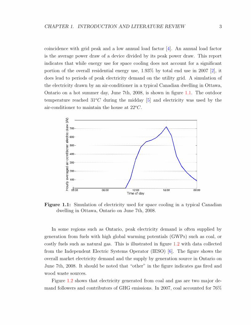
does lead to periods of peak electricity demand on the utility grid. A simulation of
the electricity drawn by an air-conditioner in a typical Canadian dwelling in Ottawa,
Ontario on a hot summer day, June 7th, 2008, is shown in figure 1.1. The outdoor
temperature reached 31oC during the midday [5] and electricity was used by the
air-conditioner to maintain the house at 22oC.
Figure 1.1: Simulation of electricity used for space cooling in a typical Canadiandwelling in Ottawa, Ontario on June 7th, 2008.
In some regions such as Ontario, peak electricity demand is often supplied by
generation from fuels with high global warming potentials (GWPs) such as coal, or
costly fuels such as natural gas. This is illustrated in figure 1.2 with data collected
from the Independent Electric Systems Operator (IESO) [6]. The figure shows the
overall market electricity demand and the supply by generation source in Ontario on
June 7th, 2008. It should be noted that “other” in the figure indicates gas fired and
wood waste sources.
Figure 1.2 shows that electricity generated from coal and gas are two major de-
mand followers and contributors of GHG emissions. In 2007, coal accounted for 76%

CHAPTER 1. INTRODUCTION AND LITERATURE REVIEW 4
Figure 1.2: Market electricity demand and supply by generation source in Ontarioon June 7th, 2008 (data sourced from IESO [6]). Note: “Other” indicates gasfired and wood waste sources.
of all fossil fuels used to generate electricity in Canada [7]. Residential space cooling
and appliance usage are significant causes of the peak electric demands that resort to
the use of these fuels. Note also that the electricity used for space cooling simulated
in figure 1.1 follows the market electricity demand and supply of the same day in
figure 1.2. Increases of up to 200% in transmission losses during peak demand [8]
compared to base level demand result in further network inefficiencies. Strategies to
reduce residential peak demand need to be explored.
One strategy to reduce peak electricity is demand side management (DSM). DSM
attempts to shift non-essential appliance activities, such as clothes washing and dry-
ing, from on-peak periods to off-peak periods. Ontario intends to implement a time of
use (TOU) program as a form of DSM. When implemented province-wide, occupants
will pay more for electricity during on-peak hours than during off-peak hours.
A pilot of the TOU program in Ontario showed an average household utility bill
savings of 3% on the program, compared to the two-tiered pricing scheme currently
in place [9]. These savings indicate that users responded to financial incentives and

CHAPTER 1. INTRODUCTION AND LITERATURE REVIEW 5
shifted a portion of their demand to off-peak times. The only month to show an
average household utility bill increase was August. It could be argued that this
increase was from air-conditioning use during on-peak times that could not be shifted
to off-peak times. This increase shows a flaw in DSM strategies. Appliances such
as ovens that cannot be shifted to off-peak times and air-conditioners that are only
effective when the outside temperature is high, coincidental with on-peak periods,
cannot be influenced by DSM. If the electricity consumed by air-conditioners and
appliances that are required during on-peak times could be produced off-peak, stored,
and used later, the objective of DSM could be realized. A study by Shaw [10] of load-
shifting in the UK showed modest network savings of 0.02%. This study, however, only
explored savings in transmission losses during peak periods by theoretically shifting
a portion of the on-peak loads to off-peak.
In order to reduce GHG emissions from peak electricity demand at the residential
level, other strategies of power production and transmission need to be explored.
Micro-cogeneration and electric storage are potential solutions.
1.2.2 Micro-cogeneration
Micro-cogeneration devices are showing promising developments for electricity gener-
ation at the residential level. These devices are generally either internal combustion
engines, solid oxide fuel cells, proton exchange membrane fuel cells, or Stirling en-
gines (SEs). They typically generate less than 10-15kW of electricity and are located
within the household. Micro-cogeneration devices may defer demand from the utility
grid.
When producing electricity alone, micro-cogeneration devices yield poor efficien-
cies, as low as 5% in net AC power with reference to the source fuel’s lower heating
value [1]. However, by using the thermal energy lost in the electrical conversion pro-
cess for domestic hot water (DHW) and space heating within the home, known as
cogeneration, the device’s efficiency improves. If done effectively, the efficiency of
these devices may be improved from 30-35% to over 80%, referenced to the source
fuel’s higher heating value [11].
Micro-cogeneration devices are being implemented worldwide. Although relatively
new, SE micro-cogeneration units in France, in 2003, yielded a primary energy savings
of 13%. Similar technologies in the UK have yielded primary energy and emissions
savings of 28% [11].

CHAPTER 1. INTRODUCTION AND LITERATURE REVIEW 6
The potential of reducing residential electric demand using micro-cogeneration
devices was assessed using whole-building computer simulation software. This as-
sessment was Annex 42 of the International Energy Agency’s Programme on Energy
Conservation in Building and Community Systems (IEA/ECBCS) [1]. It concluded
that engine start-up time, high operating temperatures, large thermal inertia, and in-
ternal controls preventing high thermal stresses, resulted in poor response to transient
electrical loading. Micro-cogeneration transient performance needs improvement to
be applied at the residential level, where electricity demand fluctuates rapidly.
A micro-cogeneration device connected to a utility grid can use the grid as an
infinite storage source. When the device is generating less electricity than is being
demanded from the household, it can import electricity from the grid to make up
the difference. The device can also export excess electricity to the grid when its
production exceeds the household demand. The excess electricity produced by a few
residential cogeneration units can be easily re-distributed through the network. How-
ever, for a high penetration rate of micro-cogeneration devices in households, the grid
can no longer be used as an infinite storage source. Consequently, storage techniques
within the household need to be explored, defined here as residential electric storage
(RES).
1.2.3 Electricity storage and lithium ion batteries
Many benefits may be achieved from the addition of electric storage. Ibrahim et
al. argue that storage could alleviate periods of peak demand, relieve grid conges-
tion, improve infrastructure and prevent power outages on catastrophic scales such
as blackouts [12].
Many energy storage techniques exist and can be classified by their type of storage:
mechanical, electrical, electrochemical, thermal and potential. Specific techniques
such as pumped hydro storage, compressed air storage, flywheel energy storage, ther-
mal energy storage, super capacitors and superconducting magnetic energy storage
have been discussed [12, 13].
Electrochemical storage using batteries has been in practice for many years, in
different forms. Primary batteries are not capable of recharging and have limited ap-
plication. Although, due to their simplicities and reliabilities, these are the most com-
mon form of battery. Secondary batteries, capable of recharging, have been present

CHAPTER 1. INTRODUCTION AND LITERATURE REVIEW 7
in vehicles in the form of lead acid (PbA) batteries. PbA battery technology is read-
ily available at low cost, and is ideal in vehicles for low power demand applications
such as starting, lighting and ignition sequences. New secondary battery technologies
such as nickel cadmium (NiCd), and nickel metal hybrides (NiMH), have been im-
plemented in electric vehicles and hybrid vehicles [14]. These batteries exhibit higher
energy and power densities than PbA batteries. These advantages have lead to the
commercialization of all these new battery types.
Another secondary battery chemistry is lithium-ion. The process of energy stor-
age in a li-ion battery can be briefly described using the schematic shown in figure
1.3. During discharging, lithium ions diffuse from the anode to the cathode across
an electrolyte separator, while releasing an electron across an external electric cir-
cuit. During charging, the process is reversed. This will be elaborated in chapter
4. Research is ongoing to improve the electrochemistry of li-ion batteries and their
performance [15, 16].
Figure 1.3: Schematic of lithium ion battery.
Li-ion batteries exhibit better characteristics compared to other secondary bat-
teries [17]. They currently exhibit capacity retention after more than 3000 cycles at
a discharge depth of 80 % [18]. This value is optimistic and is contested by some
[19]; it depends highly on the treatment, control and discharge depth of the battery.
Li-ion batteries also have low self-discharge rates of 2% to 8% per month [20]. Even at

CHAPTER 1. INTRODUCTION AND LITERATURE REVIEW 8
low states of charge (SOC), li-ion batteries can be left for extended periods without
recharging [14]. Li-ion batteries also have higher energy and power densities than
other secondary batteries [17].
Ibrahim et al. [21] uses a performance index, including cost, to determine the
optimal storage technique for a permanent application, similar to the criteria for
RES. He concludes that while li-ion batteries exhibit better performance than other
secondary batteries, they are currently too expensive. Li-ion batteries are currently
available at around $1000 USD per kWh of storage capacity [22]. Cost effectiveness
will be achieved with further development, production in mass quantities and an
increase in market competition. The United States Council for Automotive Research
LLC has set near and longterm goals for li-ion costs at $150 USD/kWh and $100
USD/kWh, respectively [23].
Along with cost, a relatively complex battery management system (BMS), in-
volving a sophisticated control must be implemented to safely modulate the battery.
Proper control of a li-ion battery is crucial to ensure high capacity retention, while
avoiding physical dangers such as fire or explosion.
Storing electricity in a rechargeable battery facilitates a quick transient response
to a varying imposed electric load. This makes micro-cogeneration systems with RES
a potential solution for small-scale power generation, at a large rate of penetration.
1.2.4 RES modelling
Micro-cogeneration models using battery storage for load levelling applications have
been developed using PbA batteries [24]. An electric storage model in the build-
ing simulation program ESP-r [25], using PbA and vanadium redox flow batteries
(VRFB) has also been developed. This model, developed by Ribberink and Wang
[26], incorporates a PbA and VRFB storage system, coupled with photo-voltaic (PV)
renewable generation, within the power modelling domain of ESP-r, described by
Clarke [27].
From the results of Annex 42 of IEA/ECBCS [1] and in conjunction with National
Research Council’s Institute for Chemical Process and Environmental Technology
(NRC-ICPET), a li-ion battery model based on the literature and previous work was
developed. This model was coupled with existing micro-cogeneration models in ESP-r
[25]. The RES model developed in this work used a “grey box approach”, practiced
extensively in engineering fields [1, 27]. This approach treats each sub-system as

CHAPTER 1. INTRODUCTION AND LITERATURE REVIEW 9
control volumes for energy transfer, and where conservation of mass and energy laws
apply. A schematic of the RES model using this control volume method is shown as
figure 1.4.
Figure 1.4: Schematic of Li-ion micro-cogeneration model.
For any simulation result to be valid, not only should the physics of the real life
system be captured, but the simulation inputs also must be accurate. In the context
of RES, one of these inputs are the electrical demands of the household.
1.2.5 Residential load monitoring
Whole building simulation software has been developed to accurately assess thermal
and electrical demands of a building. This assumes that accurate inputs for occupant
activities, such as appliance usage and lighting, have been provided. These activities
contribute to the household’s non-HVAC loads. These loads, typically applied in
simulation software as energy profiles, can have large effects on the building’s thermal
and electrical demands. Non-HVAC loads vary widely between households, depending
not only on the size and location, but on the habits, lifestyle and social status of the
occupants [28].

CHAPTER 1. INTRODUCTION AND LITERATURE REVIEW 10
Accurate data to represent typical non-HVAC loads for a wide spectrum of Cana-
dian dwellings is unavailable [1]. This makes it difficult to assess electric demands in
building simulation software. The results from Annex 42 of the IEA/ECBCS showed
that the potential for residential cogeneration is reliant on these non-HVAC loads [1].
Previous work in producing synthetically generated non-HVAC profiles for Canadian
houses using a bottom-up approach was performed by Armstrong et. al [29]. These
profiles did not include air-conditioning usage and will be discussed in further detail
in chapter 3.
Beausoleil-Morrison [30] observed that occupant intervention can have significant
impacts on space cooling. Space heating in the winter is easy to predict in building
simulation, as occupant intervention has little effect. However during the summer,
occupant intervention from opening and closing windows, blinds and shutters have
significant impacts on cooling loads by bringing in outdoor air and reducing passive
solar gains. Thermostat control strategies, chosen by the occupants, also affect space
cooling. These occupant interventions make space cooling predictions in building
simulation difficult. Further data regarding electrical usage and occupant intervention
of typical Canadian dwellings is needed to assess a RES system.
1.3 Research objectives
Canadian residential electricity usage from appliances and air-conditioners, i.e., peak
demand, leads to inefficient electricity production from increased GHG emissions.
New strategies in micro-cogeneration and electrical storage may be a solution to
reducing peak demand. These solutions, that can be assessed via building simulation,
require accurate representation of non-HVAC and air-conditioning loads for valid
results. This thesis will attempt to address the above with the following research
objectives:
• Improvement of non-HVAC electrical load profiles for Canadian households;
• Improvement of space cooling electrical profiles and their dependency on occu-
pant habits for Canadian households;
• Development of a quasi-steady-state li-ion battery model in ESP-r;
• Calibration of the li-ion model parameters with external data;

CHAPTER 1. INTRODUCTION AND LITERATURE REVIEW 11
• Demonstration of new modelling capabilities of the li-ion model coupled with a
cogeneration model within a residential house with non-HVAC and space cooling
loads; and
• Recommendations toward a full assessment and optimization of such a system,
and the metrics to measure its performance.
1.4 Thesis outline
To meet the objectives listed in the previous section, the remaining thesis will be
organized in the following fashion:
• Chapter 2 reviews the ESP-r methods used to simulate the thermal and electric
demands of a building.
• Chapter 3 reviews the non-HVAC electrical consumption data collected in a
measurement project of residential dwellings in the Ottawa area. This data will
be compared to previous methods of representing non-HVAC loads in a Cana-
dian context. The chapter also reviews the space cooling electrical consumption
data collected in the same project.
• Chapter 4 briefly reviews li-ion battery chemistry and the different approaches
in modelling this behaviour. The chapter proceeds with the development and
implementation of a li-ion battery model within ESP-r.
• Chapter 5 outlines the procedure to calibrate a li-ion battery model in ESP-r
based on specific battery chemistry, configuration, etc.
• Chapter 6 reviews the summation of the previous chapters by demonstrating
the li-ion model coupled with a micro-cogeneration model within a residential
house with non-HVAC and space cooling loads.
• Chapter 7 summarizes the results of this research and recommends future work
needed to assess a RES system.

Chapter 2
ESP-r simulation methods
The li-ion modelling research objectives could be completed using many simulation
tools. The use of numerical method software such as C++ or Matlab would first
require the modelling of the thermal, air flow, plant and electrical interactions that
occur within a dwelling. The use of building simulation software, where these inter-
actions have been previously modelled, would eliminate this problem. While other
building simulation software such as TRNSYS or EnergyPlus could have been used,
ESP-r [25] has been chosen for this work because it is a non-proprietary, open source
development software and has been extensively validated [31].
The development of ESP-r and its ability to simulate the thermal demands of
a building began in the 1970’s. Since then it has been continuously expanded and
refined by developers around the world. More facets of building simulation such as
air flow, electrical networks and plant networks have been implemented. [27].
Understanding the methods used to simulate in ESP-r is necessary for interpret-
ing its outputs, and for designing and implementing a li-ion model. The following
description of ESP-r’s methodologies are adapted from previous works that are cited
in the individual sections. Section 2.1 briefly outlines the thermal, air flow and plant
networks, while the power flow network is discussed in section 2.2.
2.1 The ESP-r thermal, air flow and plant net-
works
The following description of ESP-r’s thermal, air flow and plant networks is adapted
from Clarke [27]. ESP-r uses a finite difference approach to discretize a building into
12

CHAPTER 2. ESP-R SIMULATION METHODS 13
sections, known as zones. A zone can be a single room of a building, or several rooms
if their thermal states are assumed to be similar enough that they can be lumped
together for computational ease.
The zones are discretized into nodes. By default, each zone is discretized into
one air point node. The zone is bounded by opaque and non-opaque constructions,
i.e., walls and windows, respectively, which are also discretized into nodes. Any
homogeneous construction is discretized into three nodes: one at either surface and
one interior node. A wall made of n layers, e.g., gypsum, air gaps, brick etc., will be
discretized into 2n + 1 construction nodes.
Each node is treated as a control volume and has the laws of conservation of energy
and momentum applied over it to determine its thermal state at any time-step. In
general, the thermal storage capacity of the node with respect to time must equal the
net energy flow paths to the node and the net energy generation at the node:
mCpdT
dt= qpath net + qgen net (2.1)
where m is the mass of the wall construction or the air in the zone in kg, Cp is the
heat capacity of the wall construction or the air in the zone, in J ·kg−1 ·K−1, T is the
temperature of the wall construction or the air in the zone in Kelvin, and q is energy
transferred to the node with respect to time in Watts. Figures 2.1 and 2.2 illustrate
the energy flow paths and the energy generation considered at an air point node and
at a construction node, respectively.
For an air point node, the net energy flow paths are made up of several contri-
butions. The contribution from advective mass transfer, i.e., conservation of momen-
tum, is the infiltration from other zones, and the infiltration with the exterior through
cracks and openings. This contribution is proportional to the mass flow rate and the
temperature gradient between the zones and the exterior. For example, the advective
mass transfer contribution to air point node i of a zone, in a building model with n
zones and no connection to the exterior would be:
qnet advection =n−1∑j=1
(mj→iCp(Tj − Ti))j 6=i (2.2)
where mj→i is the mass flow rate between zone j and i, in kg · s−1. The mass flow

CHAPTER 2. ESP-R SIMULATION METHODS 14
Figure 2.1: Energy flow paths and energy generation at an air point node in ESP-r.
Figure 2.2: Energy flow paths and energy generation at construction nodes in ESP-r.

CHAPTER 2. ESP-R SIMULATION METHODS 15
rate is governed by the pressure gradient between the zones or exterior, scaled by an
advection coefficient. From the conservation of mass law, the sum of the mass flows
in a building with n zones must be zero (see eq. 2.3).
n∑j=1
mij =n∑
j=1
f(∆Pij) = 0 (2.3)
where ∆Pij is the pressure gradient between zone j and i, in kPa. The infiltration
from outside the building is specified using a schedule, either in rate of volume with
respect to time, or in air changes per hour (ACH). Recent work has introduced the
Alberta Infiltration Model (AIM) which calculates the infiltration based on pressure
gradients and wind speeds from an imposed weather file [32].
The contribution from heat transfer, i.e., conservation of energy, is the convection
from the bounded surfaces of the zone. This contribution is proportional to the
temperature gradient between the surface node and the air point node. For example,
the convective heat transfer contribution to air point node i of a zone in a building
model, bounded by m surfaces would be:
qnet convection =m∑
s=1
Ashs→i(Ts − Ti) (2.4)
where As is the surface area of surface s, in m2, and hs→i is a convection coefficient
between surface s and air point node i, in W ·m−2·K−1. There is no radiation exchange
and insignificant conduction exchange at an air point, hence, these contributions are
negligible. The net energy generation terms in equation 2.1 include any contributions
from the HVAC plant system and casual gains from occupants and appliances in
Watts. The advection and convection correlations used in the above equations are
determined from empirical observations.
Construction nodes follow the same form of equation 2.1 above. The net energy
flow paths of internal construction nodes, i.e., nodes that are not on the inner or
outer surface of a wall, are only made up of conduction from adjacent nodes. In
the case of air gaps in the wall, convection will exist as well. The net energy flow
paths of external construction nodes are made up of conduction from adjacent inner
nodes, convection from air point nodes or from the exterior, and long wave radiation
exchange with other surfaces or radiation exchange with the exterior. The conduction
through a construction, in Watts, is proportional to the temperature gradient over the
CHAPTER 2. ESP-R SIMULATION METHODS 16
construction and its material conductivity, in W ·m−1 ·K−1. A linearized radiation
coefficient hr, in W · m−2 · K−1, is used to treat the radiation exchange between a
surface s and the other surfaces in the zone:
qnet radiation =
(m−1∑i=1
Ashrs→i(Ts − Ti)
)i6=s
(2.5)
The net energy generation term in equation 2.1 for the construction nodes include
any contributions from an HVAC plant system injected into the construction in Watts.
Non-opaque surfaces, i.e., windows, are discretized in the same fashion as opaque
ones. However, in the presence of incoming solar radiation, ESP-r calculates the
amount of radiation transmitted into the zone and absorbed by the surface itself.
This is specified over several angles relative to the window. Recent work has advanced
the non-opaque surface treatment to include the effects of convection and diffusion of
thermal heat to the surface from absorbed radiation [33].
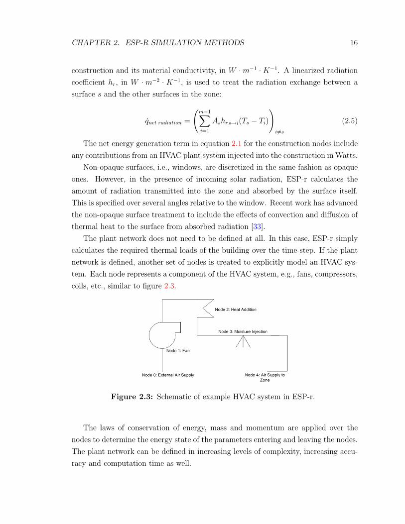
The plant network does not need to be defined at all. In this case, ESP-r simply
calculates the required thermal loads of the building over the time-step. If the plant
network is defined, another set of nodes is created to explicitly model an HVAC sys-
tem. Each node represents a component of the HVAC system, e.g., fans, compressors,
coils, etc., similar to figure 2.3.
Figure 2.3: Schematic of example HVAC system in ESP-r.
The laws of conservation of energy, mass and momentum are applied over the
nodes to determine the energy state of the parameters entering and leaving the nodes.
The plant network can be defined in increasing levels of complexity, increasing accu-
racy and computation time as well.

CHAPTER 2. ESP-R SIMULATION METHODS 17
The above equations are expanded using a first order Taylor series expansion.
This may be done using an explicit or implicit scheme, i.e., if the equations use the
previous and current time-step values (explicit), or the future and current time-step
values (implicit). Each scheme has draw backs; explicit schemes are stable but heavily
dependant on the time-step resolution, and implicit schemes tend to be unstable.
ESP-r employs a Crank-Nicolson approach which is a 50:50 weighted average of both
schemes to solve the system of equations.
Each nodal equation is arranged to create three arrays in the form A · T = B.
The matrix is closed with the boundary conditions imposed on the system, i.e., the
temperature control set-points of the zone and/or control set-points on the plant. The
A matrix contains the conduction/convection/radiation coefficients between nodes,
and the B matrix contains the boundary condition terms. The T matrix is a linear
vector of nodal temperatures and, if applicable, a net plant heat injection/removal
term. Figure 2.4 shows a thermal network set of arrays and focuses on node i, an
interior construction node with the plant contributing to its thermal state. Using
Gaussian elimination, the T vector is solved to determine the nodal temperatures
and plant contribution for the time-step.
To obtain a global solution of the nodal temperatures and plant contribution,
the different networks must be solved simultaneously. This is because several of the
parameters are needed in more than one set of equations. For example, a micro-
cogeneration device would affect the thermal, plant and power flow networks. Conse-
quently, the networks are highly coupled and various parameters are passed between.
The solution process occurs using an iterative method until all the network solutions
have converged. The interested reader is referred to Clarke [27] for more information
on the development of the networks in this section.
2.2 Electrical power flow network in ESP-r
The previous section briefly described the basic domains that ESP-r implements to
calculate the energy performance of a building. The electrical power flow network of
ESP-r need not be defined to calculate the thermal loads of the building. However,
the objectives of this research require the implementation of this network, so it is
necessary to outline its development. The following is a brief overview of the power
flow network derived by Kelly [34]. The interested reader is referred to Kelly’s thesis

CHAPTER 2. ESP-R SIMULATION METHODS 18
Figure 2.4: Matrix equations for thermal domain at ith node with plant injection.
[34] or a paper by Clarke [35] for further description of the power flow network.
The power flow network in ESP-r uses a series of nodes to represent electrical
components in a building. The network must be capable of expressing alternating
current (AC) and direct current (DC). As such, the following derivation will be in
terms of phasor values. In other words, the current and voltage are changing direction
sinusoidally with respect to time. The impedances in a network can be real (resistors),
imaginary (capacitors and inductors), or a combination of both.
Each node represents the electrical current contribution of a component over a
time-step. Kirchoff’s law that states that the sum of the currents at any node in an
electric network must be zero. Hence at node i in a network of n nodes, it follows
that: (n∑j
Iij
)j 6=i
= 0 (2.6)
where Iij is the phasor current between nodes i and j over the time-step in Ampere.

CHAPTER 2. ESP-R SIMULATION METHODS 19
An example of an electric power flow network defined in ESP-r is shown in figure
2.5.
Figure 2.5: Example of electrical network schematic in ESP-r.
In the network, components can take on one of three roles: electricity consumers,
electricity generators, and electricity transmitters. From the three types of compo-
nents above, Kirchoff’s current law in equation 2.6 still holds :(Cn∑j=1
ICij
)j 6=i
+
(Gn∑j=1
IGij
)j 6=i
+
(Tn∑j=1
ITij
)j 6=i
= 0 (2.7)
For example, figure 2.5 has two nodes defined: a node representing the grid con-
tribution and a node representing electrical interactions to the house. The grid node
has one source component, the grid itself, and one transmission component, the elec-
tricity transmitted to and from the house. From equation 2.7 above, the grid node
would reduce to:
IGgrid + IT→house = 0 (2.8)
Likewise for the house node, the generating component is the micro-cogeneration
device, the consuming component is the house’s electrical loads, and the transmitted
component is the interaction between the grid. The battery at the house node can
act as a generator or consumer depending on if the battery is charging or discharging:
IGcogen + IChouse + IC/Gbattery + IT→grid = 0 (2.9)
All the generating and consuming terms are moved to the right hand side of the
equation and Ohm’s law is substituted in the transmission terms. Ohm’s law states
that the ratio between the voltage and current, in magnitude and phase, is known as
CHAPTER 2. ESP-R SIMULATION METHODS 20
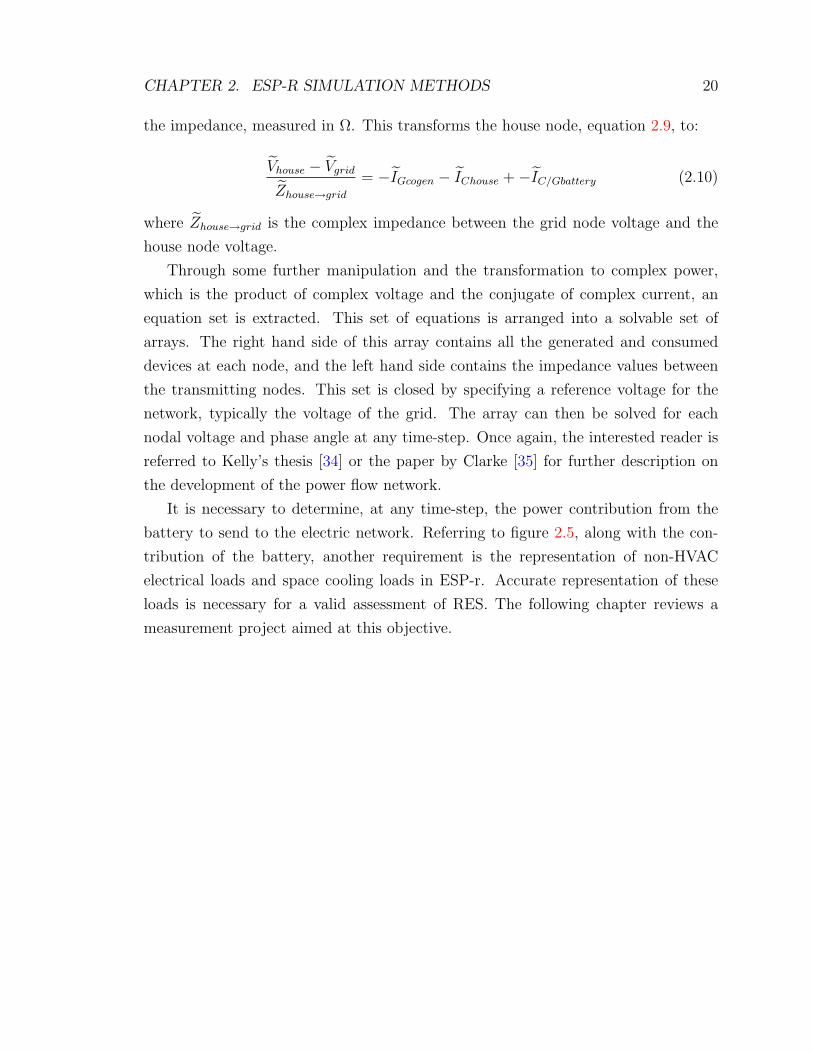
the impedance, measured in Ω. This transforms the house node, equation 2.9, to:
Vhouse − Vgrid
Zhouse→grid
= −IGcogen − IChouse +−IC/Gbattery (2.10)
where Zhouse→grid is the complex impedance between the grid node voltage and the
house node voltage.
Through some further manipulation and the transformation to complex power,
which is the product of complex voltage and the conjugate of complex current, an
equation set is extracted. This set of equations is arranged into a solvable set of
arrays. The right hand side of this array contains all the generated and consumed
devices at each node, and the left hand side contains the impedance values between
the transmitting nodes. This set is closed by specifying a reference voltage for the
network, typically the voltage of the grid. The array can then be solved for each
nodal voltage and phase angle at any time-step. Once again, the interested reader is
referred to Kelly’s thesis [34] or the paper by Clarke [35] for further description on
the development of the power flow network.
It is necessary to determine, at any time-step, the power contribution from the
battery to send to the electric network. Referring to figure 2.5, along with the con-
tribution of the battery, another requirement is the representation of non-HVAC
electrical loads and space cooling loads in ESP-r. Accurate representation of these
loads is necessary for a valid assessment of RES. The following chapter reviews a
measurement project aimed at this objective.

Chapter 3
Non-HVAC and Space Cooling Electric
Loads
Chapter 2 briefly reviewed the methods applied in ESP-r to solve the energy interac-
tions that take place in a building. The electrical network, explained in section 2.2,
will be used to assess a RES system. The validity of this assessment requires accu-
rate representation of residential electric loads in building simulation. This chapter
reviews an ongoing project in representing these loads in a Canadian context. Sec-
tions 3.2, 3.3 and 3.4 represent the contributions of this research in the gathering and
analysis of Canadian residential electricity usage.
3.1 Previous work and synthetically generated
profiles
Representing non-HVAC electrical residential loads for different countries and cli-
mates has been previously performed. The approach used to represent them generally
falls into two categories: empirical data collection at the end user level or a bottom-up
approach.
The following are some examples of empirical data collection projects occurring
worldwide. A study by Isaacs et al. at the BRANZ Group monitored 400 randomly
selected houses in New Zealand from 1997 to 2005 [36]. Each house, monitored for at
least 11 months, had the rate of each type of fuel (e.g., natural gas, electricity etc.)
entering the house recorded at 10 minute intervals. The temperature of each room
in the household was also measured. Information of the occupants’ social status and
physical properties of the house were also recorded.
21

CHAPTER 3. NON-HVAC AND SPACE COOLING ELECTRIC LOADS 22
Another study by Parker at the Florida Solar Energy Center monitored 204 res-
idences in Central Florida in 1999 [37]. This study monitored total electricity con-
sumption at 15 minute intervals, broken down into space heating, space cooling, water
heating, dryers, cooking and pool energy use.
Subtask A of Annex 42 of IEA/ECBCS [28] reviewed residential non-HVAC elec-
tricity profiles gathered around European and North American nations. Most notedly,
was the monitoring of non-HVAC profiles of 90 homes around the United Kingdom
at 5 minute intervals between 2002 and 2005. Other collaborating nations included
Switzerland, Finland, Belgium, Germany and Portugal.
Within Canada, a study by Hydro-Quebec from 1994 to 1996, measured non-
HVAC electricity demand from 57 single detached homes at 15 minute intervals [28].
Another study by Newsham at the National Research Council’s Institute for Research
in Construction (NRC-IRC) and Rowlands at the University of Waterloo [38] recorded
hourly electrical utility consumption at the household meter. It included 1297 houses
in Southeastern Ontario from 2006 to 2008, of which detailed information of the
household and occupants for 365 houses is known, 498 houses from Eastern Ontario
from 2006 to 2007, and 150 houses from Northwestern USA from 2005 to 2008.
Empirical data collection projects are the most effective way of representing non-
HVAC electric loads. However, they are often expensive and intrusive to the occupant,
making it difficult to achieve large sample populations. None of the projects above
measured non-HVAC or space cooling electricity consumption of Canadian residences
at a time resolution finer than 15 minutes.
Subtask A of Annex 42 of IEA/ECBCS [28] noted that a coarse time resolution
may fail in effectively capturing electric loads. Figure 3.1 illustrates the necessity
of having electricity usage data at a fine time resolution. The data in the figure
was collected in this work, explained in section 3.2. The figure shows the average
power drawn by the household of each minute in the day, and the same data using
hourly averaged values in the day. If the hourly curve was used for a simulation
of a cogeneration device, the device would only have to satisfy a maximum load
of 1.5 kW . If the one minute curve was used for the same simulation, the device
would have to meet several periods approaching 4 kW of electricity demand, much
closer to the household’s instantaneous electricity demand. For the assessment of a
micro-cogeneration device with RES, a temporal resolution of five minutes or less
would allow the physics of such a system to take place with sufficient resolution,

CHAPTER 3. NON-HVAC AND SPACE COOLING ELECTRIC LOADS 23
Figure 3.1: Comparison of typical electricity profile taken at one minute intervalsand averaged over one hour intervals.
whilst conserving quasi-steady-state assumptions used in modelling transient plant
performance as described by Beausoleil-Morrison [39].
The bottom-up approach is the second method for representing residential elec-
tricity usage. This approach uses statistical data of annual household electricity use
and household appliance penetration rates as inputs to an algorithm. Using stochas-
tic random number generation, electricity usage profiles are created based on the
probabilities of appliance usage applied in the algorithm.
The bottom-up approach obtains data relatively easily from energy production
by source data and census information. However, the approach relies heavily on the
accuracy of the algorithm implemented for generation. Examples of the bottom-up
approach include the works by Widen et al. in Sweden [40], Capasso et al. in Italy
[41] and Paataro and Lund in Finland [42].
As discussed in section 1.2.5, synthetically generated electricity profiles, represent-
ing the stock of Canadian households, using a bottom-up approach were developed
by Armstrong et. al [29]. The non-HVAC profiles, created at five minute intervals,
targeted three levels of annual electricity consumption: low, medium and high. These
targets were based on statistics of Canadian residential electricity use [2, 3]. Each

CHAPTER 3. NON-HVAC AND SPACE COOLING ELECTRIC LOADS 24
consumption category had three years of non-HVAC profiles produced. This work did
not include air-conditioning usage in its development. The profiles produced in this
work were validated with the dataset collected by Hydro-Quebec from 1994 to 1996
[28].
Both approaches, empirical and bottom-up, generally result in attempts to create
new profiles based on original data and the use of stochastic randomly generated
numbers. This requires the implementation of some algorithm to mimic occupant
behaviour and appliance usage. Earlier methods in this began with works by Walker
and Pokoski [43], and Gross and Galiana [44], and have recently developed into more
sophisticated algorithms using fuzzy logic, genetic algorithms and neural networks
[45]. Paatero and Lund [42] noted that these new algorithms may improve profile
accuracy where detailed statistical data is unavailable.
3.2 Electrical measurement project
To better understand Canadian residential non-HVAC and space cooling electricity
use at a fine time resolution, electric consumption data was measured in several houses
throughout Ottawa, Ontario for one year beginning in July, 2009. Measuring devices
were installed at the electric panels of twelve houses similar to the images shown
in figure 3.2. These devices individually measured the household’s overall electricity
consumption, air-conditioning consumption and furnace air circulation fan consump-
tion at one minute intervals. The households in the project obtained space heating
and DHW by other means than electricity. Thus, by subtracting the air-conditioning
and furnace fan consumption from the overall house electrical consumption, the non-
HVAC electrical consumption was known.
The households were selected in an effort to represent the wide spectrum of Cana-
dian dwellings. They were chosen to fit in one of the following annual energy con-
sumption categories: low, medium and high. These categories were taken from the
annual consumption targets used by Armstrong et. al [29] in her development of
synthetically generated profiles.
Periods of data are missing from the households throughout the year, elaborated
upon further. To determine the approximate annual non-HVAC electricity consump-
tion of a household, in kWh · yr−1, the average household electric draw from the

CHAPTER 3. NON-HVAC AND SPACE COOLING ELECTRIC LOADS 25
Figure 3.2: Measuring devices installed at the electric panel of a participant in theelectric measurement project.
available data was determined, in kW , and was assumed to have been drawn con-
stantly by the household for one year. Additionally, at the time of analysis, a full
year of data was not yet collected. More than one month of data, beginning near
the end of May 2010, was missing for each household. The approximate annual non-
HVAC electricity consumption of each house, sorted by energy consumption category,
is summarized in table 3.1.
Label Low Label Medium Label High
H1 4870 H5 5557 H9 10120
H2 2641 H6 6373 H10 8877
H3 4669 H7 5155 H11 8847
H4 5044 H8 9328 H12 11257
Table 3.1: Annual electric consumption of the participating households in kWh ·yr−1. Note that bias exists due to the lack of a complete year of collected data.

CHAPTER 3. NON-HVAC AND SPACE COOLING ELECTRIC LOADS 26
Three households, H1, H10 and H12, each had an additional three electric appli-
ances measured. These were the stove, dryer and dishwasher. This was in collab-
oration with NRC-IRC to gain a better understanding of high energy consumption
appliances in households. H10 used electricity for DHW and had this circuit moni-
tored instead of their dishwasher. All of the occupants in the project also completed
a brief survey prior to the project’s commencement. This survey included questions
about the number of occupants, their typical physical presence over the day, their
thermostat control, and their willingness to use shading and window openings to
mitigate cooling loads throughout the day.
In an oversight, one of the medium houses, labelled H8 in table 3.1, obtained
DHW from an electric heater that was not being measured. While this is still an
interesting case to study in building simulation and reducing peak electrical loads, for
the non-HVAC analysis in this chapter, this house is removed. The annual electricity
consumption reported for H8 in table 3.1 includes electricity consumed for DHW
heating.
3.2.1 Measurement methods and data analysis
Measurement methodology
Energy transducers (ETs) monitored multiple circuit phases, at a rate of four hertz,
and logged the electricity consumed by the circuit each minute. Current transformers
(CTs) were attached to a desired circuit at the electric panel. If an AC current existed
in the circuit that the CT was wrapped around, a current from the circuit’s magnetic
field would be induced in the CT. The voltage of the desired circuit, and phase angle
between the voltage and current, were also sampled. Using the current induced in
the CT, and the voltage and phase angle of the circuit, the energy consumed by the
electric circuit, in W · h, was determined by the ET using equation 3.1.
E = V Icosθ∆t (3.1)
where V and I in this equation are the root mean square of their phasor counterparts,
θ is the phase angle, and ∆t is the logging interval (1 minute).
Each CT, classified by their rating, had a specific threshold of energy consumption,
shown in table 3.2.

CHAPTER 3. NON-HVAC AND SPACE COOLING ELECTRIC LOADS 27
Rated CT Size(Amps) Watt-hours per pulse
30 0.750
50 1.250
100 2.5
Table 3.2: Watt-hours per pulse resolution in logging equipment in the measurementproject.
The rated current of the CTs on the overall household circuit was 50 A, and 30
A for the individual circuits. Household H4 in table 3.1 had 100 A CTs on its overall
circuit and 50 A CTs on its individual circuits.
If the circuit being monitored consumed this threshold of energy, a relay switch
would open in the ET. Using the sample rate of four hertz, if the relay was open over
the last sampling cycle, the logger would increase its count of open relay occurrences,
also known as “pulses”, by one. At the end of each logging interval, the total number
of pulses was registered by a data logger. Thus for a logging interval of one minute
and a sample rate of four hertz, a maximum of 240 pulses per logging interval could
be registered by the data logger. The pulses could be converted to average electricity
drawn over the last logging interval of one minute using equation 3.2.
Power(kW ) = 0.06 ·WattHoursPerPulse · PulseCounts (3.2)
Measurement uncertainty
The error on the data needs to be addressed prior to any interpretation. Using a root
sum method accepted by the American Society of Mechanical Engineers [46, 47], the
bias error on the energy measured can be determined. The equipment manufacturer
reported bias errors on the CTs, phase angle θ, and the ET. These are listed in table
3.3. The bias error reported on the ET by the manufacturer was independent of the
bias error on the CT. Hence, the root sum method was assumed to be able to assess
the error in the energy consumed by the circuit.
It should be noted that these values were for normal operation. The error increased
if the current in the circuit was out of the rated range of the CT, or if the phase angle
was too large. The acceptable current range was 10% to 130% of the rated current

CHAPTER 3. NON-HVAC AND SPACE COOLING ELECTRIC LOADS 28
Device Bias Error β
CT ± 1 % of full scale
θ ± 2 o
ET ± 0.5 % of reading
Table 3.3: Bias errors of measuring devices.
of the CT, and the acceptable phase angle was less than 60o.
According to the manufacturer, the error on the voltage, βV , was accounted for
in the error on the ET, βET . The term βET also represents error beyond bias in
the measured quantities (current, voltage and phase angle), i.e., it accounts for error
on the relay in the ET. Referring to equation 3.1, the root sum square method to
determine the overall error in the measurements is then:
βTOTAL =
[(βET )2 +
(∂E
∂IβI
)2
+
(∂E
∂θβθ
)2]1/2
(3.3)
βTOTAL =[(βET )2 + (V cosθ∆tβI)
2 + (−IV sin(βθ)∆t)2]1/2(3.4)
Thus, by taking the reading of the energy consumed over the last minute, the full
rated scale of the current, which is 50 A for the overall circuit and 30 A for individual
circuits, and the phase angle, the error on any measurement is known. Unfortunately,
the phase angle was not recorded and is difficult to assess. For typical house loads
which are purely resistive, this would be close to zero degrees, making the last term’s
contribution in equation 3.4 negligible. For complex inductive loads such as a dryer
or compressor in the air-conditioning circuit, this value would play a larger role. More
analysis into the accuracy of the equipment outside acceptable current ranges and at
high phase angles is necessary.
To illustrate, a plot of bias error as a function of power consumed is shown in
figure 3.3. This plot is for an overall household circuit, with a voltage of 240 V and a
CT with a 50 A rating attached to the circuit. The phase angle is assumed to be zero
and the CT is assumed to be measuring within its rated range. Equation 3.4 is used
to calculate the bias error on the consumed energy, in W · h, which is converted to
bias error on an assumed constant power drawn over the one minute logging interval,

CHAPTER 3. NON-HVAC AND SPACE COOLING ELECTRIC LOADS 29
in kW . Bias errors on power drawn below 1.2 kW or above 15.6 kW would be higher
than the values shown in the figure, because this would be outside the acceptable
range of the 50 A CT attached to the circuit. Again, more work in equating this
error is necessary.
Figure 3.3: Bias error as a function of average power drawn by the entire householdover one minute. Note that this is for a 240 V circuit with a 50 A CT attached,and is assumed to be working within an acceptable current range and with aphase angle of zero.
The logger also reported a bias error with respect to reported logged time. Under
normal operation of an environment temperature of 25oC, this was ± 5 seconds per
week. For the houses that needed downloading once a month (discussed further on),
this equated to a maximum bias error of ± 22.5 seconds. For the houses that were
downloaded once every two months, the bias error was ± 45 seconds. This logging
time error grew with decreasing temperature, up to ± 21 seconds per week at -20oC.
Because the majority of the houses’ electrical panels were located inside the home,
this larger bias error was not a factor.
Household H3 shown in table 3.1 had its electrical panel located in its garage.
Consequently, its bias error on the reported logged time may be larger. The reported
time stamp was truncated to the nearest minute, creating a resolution error of ± 30
seconds. Hence, the resolution error should account for the majority of the bias error
with respect to time.

CHAPTER 3. NON-HVAC AND SPACE COOLING ELECTRIC LOADS 30
Data normalization
To compare household data sets to each other, a method of expressing the data in
terms of a datum or percentage was necessary. It was thought that expressing a
household’s data as a percentage of its maximum power draw from the entire study
period would accomplish this. Upon discussion, using the household’s maximum
electrical draw was abandoned. The maximum power draw may have been too random
for a realistic datum, i.e., it occurred during a power surge or blackout.
Instead, every household power draw, in kW and at one minute intervals, was
divided by the power draw representing its 95th percentile. This was accomplished
by creating a cumulative histogram of a single household over the entire study period,
showing the frequency of the electrical draws divided into increasing bins. A cumu-
lative histogram differs from a conventional one, because each bin is the frequency of
occurrences in that bin’s range, plus the summation of occurrences below that bin.
In other words, if the frequencies are expressed as percentages of all the electrical
draws, the final bin would have a value of one, because all the draws are either in this
bin or below. An example of this is shown in figure 3.4, illustrating a household from
the project. The 95th percentile, the kW value below which 95% of all the power
draws would lie, is also shown in the figure. This percentile was selected over the
maximum power draw, i.e., the 100th percentile, because it is a high power draw of
the household that occurred repeatedly.
Data division by day type and treatment of missing data
The measured data was organized by day type, i.e., weekdays and weekends, of every
season, i.e., winter, spring, summer and fall. This way, seasonal occupant driven
trends could be noticed. The weekends were considered to be Saturdays and Sundays
and the weekdays were from Monday to Friday. The beginning of spring, summer,
fall and winter was considered to be March 21st, June 21st, September 21st and
December 21st, respectively.
The data from the houses that were only measuring the overall, air-conditioning
and furnace fan circuits needed to be downloaded every two months. The data from
the houses measuring the additional appliances needed to be downloaded every month.
During this downloading period of several minutes, the equipment did not log any
data, creating a gap in the data sets. Rather than removing these days of useful

CHAPTER 3. NON-HVAC AND SPACE COOLING ELECTRIC LOADS 31
Figure 3.4: 95th percentile illustration from a cumulative histogram from the dataproject.
data, the several missing minutes were replaced with the same minutes from another,
randomly selected, similar day type, e.g. winter weekday.
Periods of malfunctioning equipment and/or maintenance also existed creating
larger gaps in the data sets. In these instances, the affected days were removed from
the data set for analysis.
Measurement resolution and data smoothing
Each CT, classified by its rating, had to be sized to the circuit that it was measuring.
If the circuit was consuming enough electricity that the relay in the ET was constantly
open, the CT rating was too small and could potentially miss consumed electricity.
On the other hand, if a circuit was not consuming enough electricity for the rated size
of the CT, it would not produce a magnetic field large enough to induce a current in
the CT.
This introduced an issue for measuring circuits of devices that had large variations
in power draws. This was seen in air-conditioners and furnace fans not in full oper-
ation. During the periods of low power draw, the logger would show several minutes
of no power drawn by the device. Eventually, enough energy would be consumed by
the device to open the relay in the ET, and it would seem that a sudden increase of
power was drawn by the device in that minute.
CHAPTER 3. NON-HVAC AND SPACE COOLING ELECTRIC LOADS 32
When subtracting the air-conditioners and furnace fans from the overall circuit
to produce non-HVAC profiles, this resolution issue occasionally produced slightly
negative electrical draws. These occurred when the overall household power draw
was low, and the ET relays on the smaller devices were not opening in the same
minute as the ET relay on the overall household.
To represent a more realistic power draw of devices in low power operation, the
periods of coarse resolution were treated using a special algorithm. This algorithm
searched through the original data sets, in terms of pulses, for minutes that recorded
a value of zero followed by minutes with more zeros or a single minute with a value
of one, to determine periods of coarse resolution. The number of minutes in a period
that had a value of one occur was divided by the number of minutes in the entire
period, to arrive at the average electricity drawn by the device. This is shown graph-
ically in figure 3.5. This figure shows a furnace fan not in operation throughout the
day except for a small period past 18:00. The furnace fan draws around 5 W after
being “smoothed”, compared to the original data which seemed to indicate that it
sporadically drew 44 W in one minute after several minutes of drawing no power.
This 5 W could be attributed to the furnace fan control system’s quiescent power
consumption which is the power drawn by the device when in standby. However, at
this low of current the accuracy on the measurement makes this inconclusive. The
purpose of the smoothing was to obtain realistic non-HVAC electric power draws
when subtracting the air-conditioning and furnace power draws from the household’s
overall power draw.
Data aggregation
The data was aggregated in several different time-steps, namely: five, fifteen and one
hour. This was done by averaging the power draws over the desired time-step. The
purpose of this was for further validation with previously developed work, and to
present the data, where needed, more concisely.
3.3 Non-HVAC data results
As discussed earlier, the household labelled H8 was removed from the analysis because
their DHW was electrically heated and not monitored so their true non-HVAC loads

CHAPTER 3. NON-HVAC AND SPACE COOLING ELECTRIC LOADS 33
Figure 3.5: Example of data “smoothing” as a result of too coarse of a measuringresolution for a one minute logging interval.
were unknown. It should be noted again that at the time of analysis, a full year’s
worth of data was not available and the following lacks detailed data for more than
a month beginning slightly after May 2010. All the data presented is in local time of
the household, i.e., the time shown includes daylight savings time.
The 95th percentile non-HVAC electrical power draw of the households are sum-
marized in table 3.4. These are compared with the 95th percentile non-HVAC elec-
trical power draw of the synthetically generated profiles from Armstrong et. al [29]
shown in table 3.5. It should be noted that the houses that are labelled in 3.4 are ac-
tual households in the Ottawa area and in no way relate to the synthetically generated
profiles that are labelled in table 3.5.
Table 3.4 illustrates that the 95th percentiles of the households from this measure-
ment project are not close to eachother. However, the generated profiles’ values in
table 3.5 are close to each other because they were derived using the same algorithm
with the same target annual consumption. It should be noted that the houses from
the measurement project in no way relate to the generated profiles.
The 95th percentiles from the houses monitored in the project do not increase with
the increasing energy categories shown in table 3.4; e.g., some of the 95th percentiles
of the houses in the low energy category are higher than the 95th percentiles in the

CHAPTER 3. NON-HVAC AND SPACE COOLING ELECTRIC LOADS 34
House Label Low (kW) House Label Medium (kW) House Label High (kW)
H1 2.168 H5 1.416 H9 5.356
H2 0.945 H6 1.791 H10 2.8650
H3 1.567 H7 1.327 H11 2.3936
H4 2.388 H12 3.435
Table 3.4: 95th percentile non-HVAC electrical power draw of the households in themeasurement project sorted by annual energy consumption level at one minuteintervals.
House Label Low (kW) House Label Medium (kW) House Label High (kW)
S1 1.92 S4 2.96 S7 4.67
S2 1.91 S5 2.95 S8 4.68
S3 1.93 S6 2.92 S9 4.67
Table 3.5: 95th percentile non-HVAC electrical power draw of the syntheticallygenerated profiles by Armstrong et. al [29] sorted by annual energy consumptionlevel.
medium energy category. This indicates that houses reach the electric power draw
representing their 95th percentiles in a manner that is not proportional to their total
electricity consumption.
Figures 3.6 and 3.7 show households H12 and H10’s electricity consumption on
a randomly selected hot day, Aug 11, 2009, respectively. The figures show the over-
all electricity power draw, labelled mains, the air-conditioner electricity power draw
and the dryer electricity power draw. These two devices are the largest electricity
consumers within the household.
These figures show the variance in daily electricity power draw between houses.
H10 had a baseload two to three times larger than H12 over the day. Also, there
is a significant increase of overall electricity draw in both households when the air-
conditioner and dryer are in operation. When both of these devices were in use, along
with the other household appliances, the overall house electricity draw grew from a

CHAPTER 3. NON-HVAC AND SPACE COOLING ELECTRIC LOADS 35
Figure 3.6: Household H12’s electricity use at one minute intervals on Aug. 11,2009.
baseload of approximately 0.7 kW to 9 kW in H12 and 1.8 kW to 13 kW in H10.
These are clear examples of peak power electricity draw in residential houses.
Figure 3.8 show the seasonal variation of average electrical load between houses.
Each plot shows the average daily non-HVAC electricity power draw of all the house-
holds in the project, separated by their energy category. These averages were pro-
duced by taking the data from every day in the season, including both weekends and
weekdays. Overlayed on the summer and winter plots is the OPA’s weekday TOU
periods of low, medium and high electricity demand [9]. While the winter on-peaks
coincide well with this sample population’s household demand, the summer does not
seem to. Note though that these plots do not include the space cooling electrical
power draw which would increase household electricity consumption in the midday of
the summer plot.
Figure 3.9 shows household H1’s average daily non-HVAC electrical power draw
over every summer weekday, plotted with two randomly selected summer weekdays.
This figure illustrates the detail that would be lost in averaging multiple days of
data. When averaged, the electricity peaks and lows tend to cancel each other out
and produce a trend with little variation with respect to its previous time-step. The
average curve’s peak power draw does not exceed 3 kW , whereas the daily maximum

CHAPTER 3. NON-HVAC AND SPACE COOLING ELECTRIC LOADS 36
Figure 3.7: Household H10’s electricity use at one minute intervals on Aug. 11,2009.
peaks were more than 7 kW and 10 kW for days one and two, respectively. Aver-
aging inherently defeats the purpose of analyzing peak residential loads and is not a
good statistical peak demand estimator. However, averaging is effective in identify-
ing trends of general energy consumption, i.e., baseloads and other periods for TOU
schemes.
Plotting the standard deviation of electrical loads throughout the day may effec-
tively illustrate the variation in residential loads. An illustration of this is shown in
figure 3.10. This figure shows the daily household non-HVAC electricity power draw
standard deviation using all the collected data for each house, separated by energy
category. It illustrates that the variation of electrical loads of all the households is
relatively low overnight and increases throughout the day, reaching a peak at around
suppertime. The magnitude of the deviation scales by the energy consumption of the
household, i.e., high, medium or low.
Another approach to analyze the distribution of electrical draws throughout the
day may be to produce histograms. The data was aggregated to five minute intervals
and normalized by the household’s 95th percentile as described in section 3.2.1. A
normalized histogram of each five minute interval of the day, from all the collected
data, would express the percentage of days that the household electric draw occurred

CHAPTER 3. NON-HVAC AND SPACE COOLING ELECTRIC LOADS 37
Figure 3.8: Daily average non-HVAC electricity power draw of all the households inthe project, separated by their energy category, by season in kW at one minuteintervals.

CHAPTER 3. NON-HVAC AND SPACE COOLING ELECTRIC LOADS 38
Figure 3.9: Household H1’s average non-HVAC household daily electricity drawplotted with two randomly selected days.
in a given bin. This is also the probability distribution of the magnitude of electrical
loads for that five minute interval. This is illustrated in figure 3.11 showing the
normalized histogram of household H6’s summer weekday non-HVAC electrical power
draw between 0:00 and 0:05 in the morning. Referring to the figure, from the data
collected for this household on a summer weekday between 0:00 and 0:05 in the
morning, 19% of the days had a non-HVAC electrical draw occur around 0.1 or below
of the household’s 95th percentile and 27% of the days had a non-HVAC electrical
draw occur around 0.2 of the household’s 95th percentile, etc.
The normalized histogram of each five minute interval from all the collected data
for one household was separated by bin value. A new plot was created showing each
bin with 288 bars beside each other, one bar from each of the five minute interval
histograms that corresponded to the bin. The 288 bars, making up an entire band
for one bin, represents the number of days, in percentage, that the household drew
the amount of electricity represented by that bin at every five minute interval.
A plot comparing the three medium households from the project compared to the
three medium synthetically generated profiles from Armstrong et. al [29] using the
normalized histogram approach above is shown in figure 3.12. The plot shows the
distribution of household non-HVAC electrical power draws at any five minute interval

CHAPTER 3. NON-HVAC AND SPACE COOLING ELECTRIC LOADS 39
Figure 3.10: Daily household non-HVAC electricity power draw standard deviationusing all the collected data for each house, separated by energy category.
on summer weekdays. The bins are fractions of the household’s 95th percentile,
ranging from 0.5 to 3.0. To clarify, for household H5 of the project between 0:00 and
0:05 in the morning (represented by the colour band on the top-left of the figure),
88% of the days had a non-HVAC electric draw occur around 0.5 and below of its
95th percentile, 10% of the days had a non-HVAC electric draw occur around 1.0 of
its 95th percentile and 1.2% of the days had a non-HVAC electric draw occur around
1.5 of its 95th percentile, etc.
The bands provide an intuitive validation of household loads throughout the day.
In the night time, a household typically has no appliances in operation, so the majority
of household electric power draws at these five minute intervals will occur at low
bins. In the morning, and throughout the day, non-HVAC activity increases, so the
occurrence of electrical draws in the low bins decrease, and shift to higher bins. Over
supper time, non-HVAC activity is at its highest and the occurrence of electrical
draws is at higher fractions of the household’s 95th percentile. In other words, the
shape of the bands at the higher bins should be the inverse to the shape at the lower
bins.
In comparing the data from the measurement project (shown on the top of figure
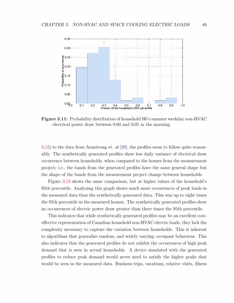
CHAPTER 3. NON-HVAC AND SPACE COOLING ELECTRIC LOADS 40
Figure 3.11: Probability distribution of household H6’s summer weekday non-HVACelectrical power draw between 0:00 and 0:05 in the morning.
3.12) to the data from Armstrong et. al [29], the profiles seem to follow quite reason-
ably. The synthetically generated profiles show less daily variance of electrical draw
occurrence between households, when compared to the houses from the measurement
project; i.e., the bands from the generated profiles have the same general shape but
the shape of the bands from the measurement project change between households.
Figure 3.13 shows the same comparison, but at higher values of the household’s
95th percentile. Analyzing this graph shows much more occurrences of peak loads in
the measured data than the synthetically generated data. This was up to eight times
the 95th percentile in the measured houses. The synthetically generated profiles show
no occurrences of electric power draw greater than three times the 95th percentile.
This indicates that while synthetically generated profiles may be an excellent cost-
effective representation of Canadian household non-HVAC electric loads, they lack the
complexity necessary to capture the variation between households. This is inherent
to algorithms that generalize random, and widely varying, occupant behaviour. This
also indicates that the generated profiles do not exhibit the occurrences of high peak
demand that is seen in actual households. A device simulated with the generated
profiles to reduce peak demand would never need to satisfy the higher peaks that
would be seen in the measured data. Business trips, vacations, relative visits, illness
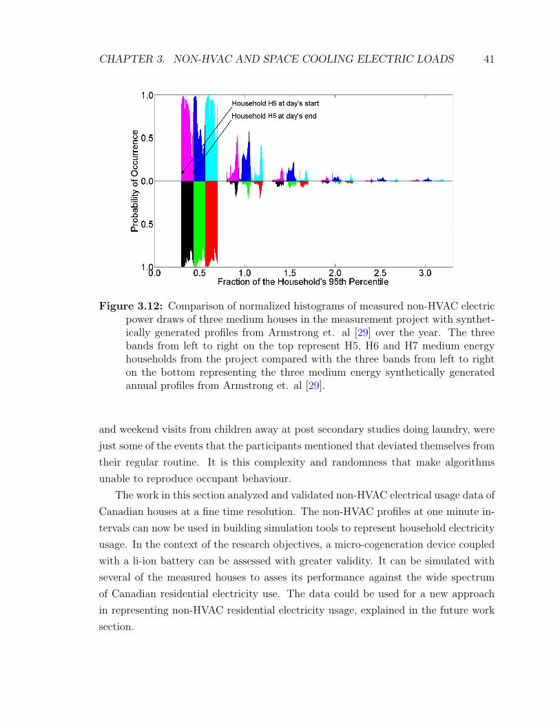
CHAPTER 3. NON-HVAC AND SPACE COOLING ELECTRIC LOADS 41
Figure 3.12: Comparison of normalized histograms of measured non-HVAC electricpower draws of three medium houses in the measurement project with synthet-ically generated profiles from Armstrong et. al [29] over the year. The threebands from left to right on the top represent H5, H6 and H7 medium energyhouseholds from the project compared with the three bands from left to righton the bottom representing the three medium energy synthetically generatedannual profiles from Armstrong et. al [29].
and weekend visits from children away at post secondary studies doing laundry, were
just some of the events that the participants mentioned that deviated themselves from
their regular routine. It is this complexity and randomness that make algorithms
unable to reproduce occupant behaviour.
The work in this section analyzed and validated non-HVAC electrical usage data of
Canadian houses at a fine time resolution. The non-HVAC profiles at one minute in-
tervals can now be used in building simulation tools to represent household electricity
usage. In the context of the research objectives, a micro-cogeneration device coupled
with a li-ion battery can be assessed with greater validity. It can be simulated with
several of the measured houses to asses its performance against the wide spectrum
of Canadian residential electricity use. The data could be used for a new approach
in representing non-HVAC residential electricity usage, explained in the future work
section.

CHAPTER 3. NON-HVAC AND SPACE COOLING ELECTRIC LOADS 42
Figure 3.13: Comparison of normalized histograms of measured non-HVAC electricpower draws of three medium houses in the measurement project with synthet-ically generated profiles from Armstrong et. al [29] at higher fractions of thehousehold 95th percentile. The three bands from left to right on the top rep-resent H5, H6 and H7 medium energy households from the project comparedwith the three bands from left to right on the bottom representing the threemedium energy synthetically generated annual profiles from Armstrong et. al[29].
3.4 Space cooling data analysis
Space cooling, while technically an HVAC electrical load, shares many similarities
with non-HVAC electric loads. Particularly, the use of air-conditioners is highly
dependant on the habits and lifestyles of the household’s occupants. As discussed
in section 1.2.5, Beausoleil-Morrison [30] observed that occupant interventions to
control the household temperature through openings and shading within the home
have significant impacts on space cooling. Occupants can program their thermostats
with different strategies throughout the day to alter these loads further. This concept
is illustrated in figure 3.14, showing the air-conditioning electricity use over the day of
three of the participants in the project on August 17th, 2009. These three households
were chosen to show the difference in air-conditioning usage between households.

CHAPTER 3. NON-HVAC AND SPACE COOLING ELECTRIC LOADS 43
The mean temperature in Ottawa that day was 25.6oC as reported by Environment
Canada’s Weather Office [5].
Figure 3.14: Example of air-conditioning variation between households on August17th, 2009 with a mean outdoor temperature of 25.6oC [5].
What this figure shows is that despite being subjected to the same conditions,
all three houses were cooled in different ways. Household H3 was cooled throughout
the day and overnight, H9 was only cooled overnight and H1 did not use their air-
conditioner this day at all. In this sense, space cooling resembles more of a non-HVAC
load, in that it relies on the complexity of its users for its function and thus, is difficult
to predict in building simulation. It is important to understand space cooling end
use, beyond penetration rates of air-conditioners, in order to determine their impact
on peak electric demand on the grid. By penetration rates, it would seem that all
the three houses in figure 3.14 would contribute to the peak electric demand on that
day. However, by collecting end user data, it is shown that each of the houses used
their air-conditioners in unique ways.
Figure 3.15 shows the increase in household electricity consumption during the
summer months due to air-conditioning of one of the houses in the project, H6. Each
bar represents the overall electricity consumption (non-HVAC and space cooling), in
kW · h, in each month. The months of July and August see noticeable increases of

CHAPTER 3. NON-HVAC AND SPACE COOLING ELECTRIC LOADS 44
total household electricity consumption. Note that some data from June was not
available and these days were replaced with available data from around this time.
Figure 3.15: Example of monthly electricity consumption of one of the houses inthe project, H6.
To explore the relationship between space cooling and outdoor temperature, scat-
ter plots were generated from the collected data. The daily electricity consumed by
each household’s air-conditioner was plotted as a function of maximum daily tem-
perature and mean daily temperature gathered from Environment Canada’s Weather
Office [5]. This plot is shown as figure 3.16. Note that the furnace circulation fan’s
electricity consumption was not included in this plot.
From this figure, there is a clear relationship between outdoor temperature and
space cooling energy consumed over the day. At hourly temperature values over the
day, this relationship would be lost. Figure 3.14 showed that occupants used their
air-conditioners at different times throughout the day, sometimes even at night.
From the plot of air-conditioning consumption (see fig. 3.16), there is a differ-
ence in air-conditioning usage between energy categories. The low energy households
tended to have lower daily space cooling electricity consumption than other house-
holds. In fact, it appears that even on some of the days with the highest maximum

CHAPTER 3. NON-HVAC AND SPACE COOLING ELECTRIC LOADS 45
Figure 3.16: Household air-conditioning unit daily electrical consumption as a func-tion of maximum and mean daily temperature. Note: Circulation fan electricityconsumption is not included in this plot.

CHAPTER 3. NON-HVAC AND SPACE COOLING ELECTRIC LOADS 46
daily temperatures, H4 resisted space cooling. This household compared to H10, for
instance, shows significant differences in air-conditioning usage.
Building simulation tools, given proper inputs such as non-HVAC loads, should
be able to accurately predict a household’s heating and cooling demands; however as
described, this becomes complicated in the cooling season with occupant mitigation
via openings and shading. The household occupants in the project also filled out a
brief survey of their willingness to open windows or use shadings to reduce their space
cooling demand, as well as their thermostat setpoints throughout the seasons. The
data collected and survey information provides excellent validation data to compare
simulation results with. By incorporating probabilities and random number genera-
tion into building simulation to mimic occupant behaviour, space cooling prediction
accuracy with building simulation may increase. This concept will be elaborated in
the future work section.
The non-HVAC data collected in this project provides excellent input data for
building simulation tools of Canadian residential electric loads. Using this data,
HVAC systems designed to meet a household’s energy demands can be more ac-
curately assessed. The space cooling data represents real information of the wide
spectrum of space cooling usage in Canadian residential homes during the summer.
Using more sophisticated algorithms to mimic occupants’ use of openings and shading
may more accurately represent true occupant behaviour in building simulation. The
space cooling data provides excellent validation for future work in this area. All the
data collected in this project will be presented using Microsoft Excel sheets, providing
specific details of each household and information about treatment of data, e.g., miss-
ing data, smoothing, etc. The gap of accurately representing residential electricity
use in building simulation to assess a micro-cogeneration device with RES has been
treated. The next research objective in this work, the development of a li-ion battery
model in ESP-r, can proceed and is discussed in the following chapter.
Chapter 4
Lithium-ion battery model
Following the adequate treatment of residential non-HVAC and space cooling electric
loads in the previous chapter, a household can be successfully modelled in ESP-r.
This model can now accurately simulate the thermal and electric demands of the
household, and can assess an HVAC plant system designed to meet these demands in
an efficient manner. This chapter discusses the next research objective of developing
a li-ion battery model in ESP-r.
4.1 Lithium-ion battery chemistry
The chemical process in a li-ion battery is known as reduction oxidation (redox).
Redox is a term given to any chemical process where atoms change oxidation states,
i.e., they lose or gain an electron. This term covers many processes including all
battery types, fuel cells, corrosion, etc.
The redox process in a li-ion battery involves the diffusion of lithium ions across
an electrolyte when an external electric load is applied to its terminals [48]. These
ions, originating from the anode with a high chemical potential, diffuse across the
electrolyte towards the cathode with a low chemical potential. In doing so, an electron
is passed not through the electrolyte, but via the external circuit to satisfy the imposed
electric load. The diffusion process is driven by the difference in chemical potential
between the anode and the cathode. This difference is the open circuit voltage (OCV)
of the battery, or the maximum potential that the battery can deliver. It is the voltage
measured across the terminal when no load is applied, i.e., when an open circuit exists
(see eq. 4.1).
47
CHAPTER 4. LITHIUM-ION BATTERY MODEL 48
OCV = µanode − µcathode (4.1)
where µanode and µcathode are the chemical potentials of the anode and cathode, re-
spectively, in Volts. The cathode of a li-ion battery is typically lithium intercalated
with a metallic oxide. These metallic oxides include nickel, cobalt and manganese.
The anode is typically a composition of lithium with carbon or graphite. During
a discharge or charge, two half-reactions take place at the cathode and anode. For
example, a li-ion battery with carbon at the anode and cobalt at the cathode would
take on the following chemical half-reactions in discharge:
Li0.45C6 → 6C + 0.45Li+ + 0.45e− (4.2)
Li0.55CoO2 + 0.45Li+ + 0.45e− → LiCoO2 (4.3)
The electrolyte needs to facilitate the diffusion of ions, but be electrically insulated,
as to not allow a short circuit or self-discharge. For PbA and NiMH, the electrolyte
has typically been an aqueous salt. However, due to the high reactivity of lithium to
moisture, the use of an aqueous electrolyte is not possible. Hence the electrolyte is
made up of a non-aqueous compound, typically lithium hexafluorophosphate, LiPF6.
Recent progress has investigated the use of a solid electrolyte polymer and the creation
of a new battery type: the lithium polymer. The interested reader is referred to Dell
[49] for more information on li-ion components and their evolution.
A large scale battery is made up of individual cells that are connected in series
or parallel. Each cell has its own chemical potential difference and capacity, which
is its available energy in W · h. When cells are connected in series, their potentials
are summed together, i.e., the overall voltage of the battery is the summation of the
individual cell potentials; but the capacity remains that of a single cell. When cells
are connected in parallel, the voltage remains the same as the lowest cell potential,
but the capacity of the battery becomes the summation of each cell capacity. This
introduces another consideration of cell balancing in the battery management system
(BMS) of a li-ion battery. Each cell potential and capacity must stay balanced with
the other cells in the pack. If one cell passes out of a safe operating range, the entire
battery pack must be shut off by the BMS, losing the remaining available capacity.
The BMS may continue operation, and risk damaging the cells that are out of safe
CHAPTER 4. LITHIUM-ION BATTERY MODEL 49
operating range which could cause harm to the battery’s environment.
State of charge (SOC) is the amount of capacity remaining in the battery, relative
to a full battery. A SOC of 100% is thus a full battery. Depth of discharge (DOD)
is the opposite of SOC, and the percentage of the battery capacity that has been
discharged. The values of SOC and DOD describe the amount of lithium that has
diffused from the anode to the cathode and depending on the manufacturer’s defini-
tion, may not account for all of the lithium in the cells of a battery. Consequently,
a cell, and hence a battery, may be able to be charged beyond a DOD of 0% (SOC
of 100%), and discharged beyond a DOD of 100% (SOC of 0%). However, this may
indicate unsafe ranges of operation to the manufacturer. Typically, the region of safe
operation of a cell exists between a DOD of 0% to 80% [49].
As more lithium ions diffuse through the electrolyte from the half reactions in
equations 4.2 and 4.3, the chemical potential rises in the anode and drops in the
cathode causing the difference between the two to dwindle. At this point, the potential
difference cannot drive the diffusion process; the cell’s capacity has been exhausted
and can no longer satisfy an imposed electric load. The OCV of a cell gradually
decreases due to changing chemical potentials, making the OCV a good measurement
of a cell’s SOC. Typical OCV for a lithium ion cell begins at 4.0 V, for a fully charged
cell, and drops to 3.0 V, for an empty one [49]. Any higher or lower and the cell risks
being in dangerous operating ranges. These values vary slightly for different li-ion
chemistries. A plot of the OCV as a function of DOD is important in the modelling
of any battery chemistry, and each chemistry has a unique shape. A li-ion cell takes
on the characteristic shape shown in figure 4.1. By accurately measuring the OCV of
a battery, or its individual cells, it is possible to obtain its remaining capacity.
The rate at which the lithium ions diffuse is governed by the magnitude of the
external load applied. The rate, in Ampere, that a cell will discharge at, is the
power demanded, in Watts, divided by the cell potential, in Volts. Cells are typically
charged and discharged at either constant power or current. To remain at a constant
power during discharge, the current must be continuously increasing because the cell
potential decreases as battery capacity decreases. Likewise, for a constant current
discharge, the imposed load continuously decreases, directly proportional to the cell
potential.
When the cell undergoes charging, an external power source is applied across the
terminals, driving the lithium ions back from the cathode to the anode. Because by

CHAPTER 4. LITHIUM-ION BATTERY MODEL 50
Figure 4.1: Open circuit voltage (OCV) as a function of DOD (1-SOC) for a lithiumion cell at 25oC. [48]
definition, an anode is the component losing ions and electrons and a cathode is the
one receiving, in a charging process the components switch and the anode becomes
the cathode and vice versa.
The internal losses of a battery or cell constitute energy capacity lost during dis-
charging, or excess energy needed during charging. They are affected by the rate
of charge/discharge and the battery temperature [50]. Losses exist in two forms:
electronic resistance and ionic resistance. Electronic resistance encompasses material
resistances of the cell’s metal components and terminal contact points. Ionic resis-
tances occur due to complex reactions at the electrochemical level. They include
electrolyte conductivity, ion mobility and electrode surface area [51]. Worth noting
in electrolyte conductivity, is the formation of the solid-electrolyte interphase. This
is the creation of a solid film on the surfaces of the electrodes in contact with the
anode and cathode during the redox process. This represents a loss of original battery
capacity and an increase in resistance [52].
While the OCV of a cell is the maximum voltage that could be delivered during
discharge, the actual voltage that is delivered to the load is always lower and decreases
linearly with current. These losses occur due to increases in kinetic reactions at the
electrochemical level. The cell is limited to a maximum current that it can charge
or discharge at without causing irreparable damage. The capacity of the cell also
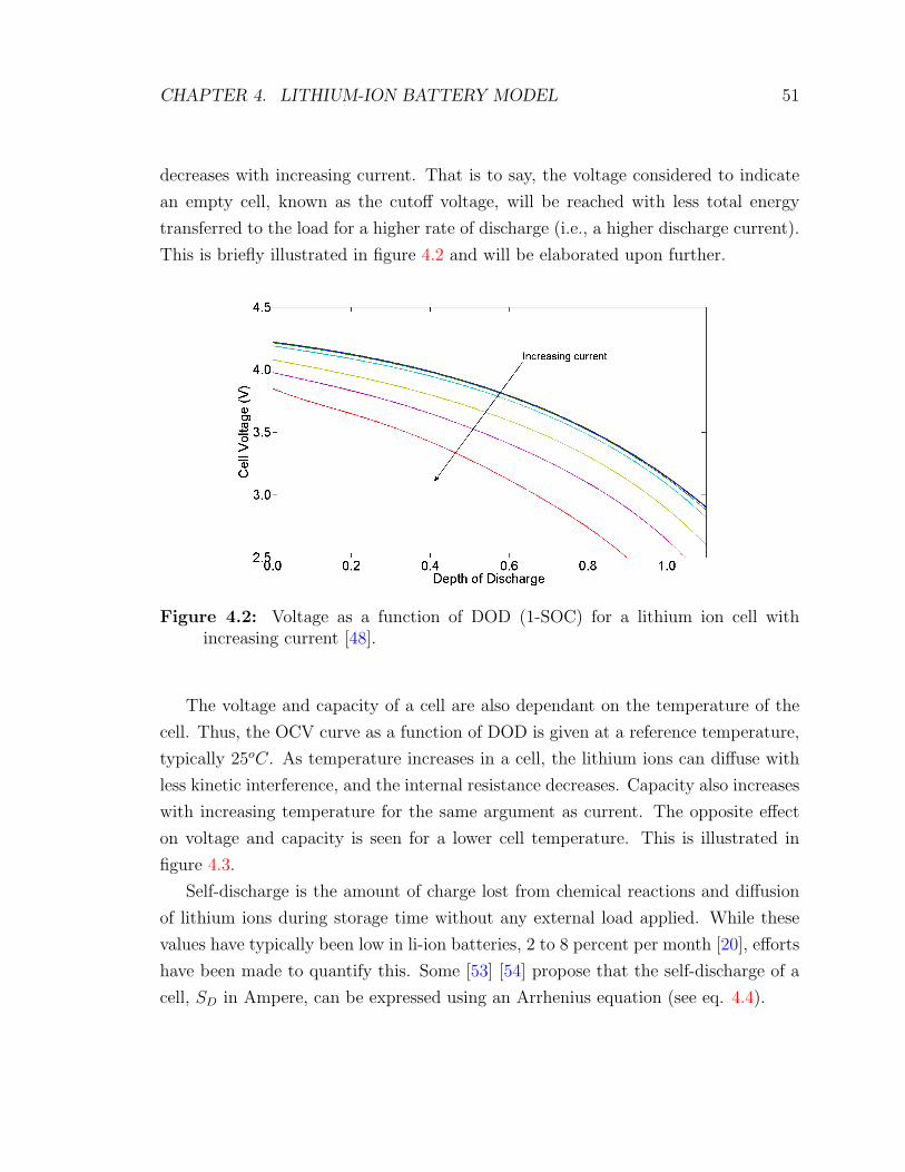
CHAPTER 4. LITHIUM-ION BATTERY MODEL 51
decreases with increasing current. That is to say, the voltage considered to indicate
an empty cell, known as the cutoff voltage, will be reached with less total energy
transferred to the load for a higher rate of discharge (i.e., a higher discharge current).
This is briefly illustrated in figure 4.2 and will be elaborated upon further.
Figure 4.2: Voltage as a function of DOD (1-SOC) for a lithium ion cell withincreasing current [48].
The voltage and capacity of a cell are also dependant on the temperature of the
cell. Thus, the OCV curve as a function of DOD is given at a reference temperature,
typically 25oC. As temperature increases in a cell, the lithium ions can diffuse with
less kinetic interference, and the internal resistance decreases. Capacity also increases
with increasing temperature for the same argument as current. The opposite effect
on voltage and capacity is seen for a lower cell temperature. This is illustrated in
figure 4.3.
Self-discharge is the amount of charge lost from chemical reactions and diffusion
of lithium ions during storage time without any external load applied. While these
values have typically been low in li-ion batteries, 2 to 8 percent per month [20], efforts
have been made to quantify this. Some [53] [54] propose that the self-discharge of a
cell, SD in Ampere, can be expressed using an Arrhenius equation (see eq. 4.4).

CHAPTER 4. LITHIUM-ION BATTERY MODEL 52
Figure 4.3: Voltage as a function of DOD (1-SOC) for a lithium ion cell withincreasing temperature [48].
SD = k0e−EASRgT (4.4)
where EAS is the activation energy of the reaction in kJ · kmol−1, Rg is the gas
constant in kJ · kmol−1K−1, T is the temperature of the cell in Kelvin and k0 is a
constant in Ampere.
Battery degradation due to cycling is the loss of initial capacity over time with
repeated charging and discharging. This is a complex quantity to define that depends
on how far the battery has been discharged, how far the battery has been recharged,
the rate at which this is done and the battery temperature [54]. Spotnitz [55] describes
this loosely using a diagram of battery capacity as a function of the number of cycles
used, shown as the left plot in figure 4.4.
In this figure, battery capacity decreases sharply over the beginning of the bat-
tery’s life (region A) and tapers off as the number of cycles increase until the end of
region C. At this point, the battery’s capacity has been reduced to about 80% of its
original, and the battery is considered to be at the end of its operable life. After this
point, the capacity will decrease at an increasing rate (region D). Spotnitz [55] states
that data on region D is hard to find as manufacturers tend to suppress this informa-
tion. This relationship between capacity and cycle life can be linearly approximated

CHAPTER 4. LITHIUM-ION BATTERY MODEL 53
Figure 4.4: Diagram of remaining battery capacity as a function of cycle life asdescribed by Spotnitz [55] (left) and approach used later in li-ion model (right).
as shown in the second plot of figure 4.4. This will be revisited in later chapters.
The development of an accurate li-ion battery model requires the modelling of all
the points discussed above. That is, the ability to capture internal resistance as a
function of current and temperature, self-discharge of a battery and long term battery
degradation while keeping the battery balanced and in safe operating limits.
4.2 Lithium-ion battery modelling
Finite difference approach
There are several different approaches to battery modelling, each having their own
benefits and limitations. The finite difference approach is the highest level of resolu-
tion. This approach involves the discretization of the anode, cathode and electrolyte
of a li-ion cell. By applying the laws of conservation of mass, momentum and energy,
the diffusion of lithium ions through these discretized nodes, driven by the chemical
potential gradient between the anode and cathode, is modelled. The model can be
specified in all spatial coordinates and unsteady temporal frames. This approach is
closely based on Fick’s law of diffusion [56]:
mA
A= − ~D · ∇CA (4.5)
where mA
Ais the mass flow rate with respect to time per area, D is a proportionality
diffusion coefficient in area per time, and CA is a mass concentration per volume.

CHAPTER 4. LITHIUM-ION BATTERY MODEL 54
The largest advantage to this approach is the ability to accurately capture the
true behaviour of a battery’s internal resistance, essentially its efficiency, by apply-
ing different boundary conditions. This includes the relationship of resistance with
current and temperature, other phenomena such as impurities in the manufacturing
process, which may lead to ion concentrations on the electrode surfaces, and realistic
long-term battery degradation. Limitations to this approach are the same experi-
enced in conventional computational fluid dynamics. These include the truncation
of higher order terms in Taylor series expansion, etc. Another limitation is the lack
of empirical data, specifically in terms of life cycle degradation, to apply realistic
boundary conditions to the model. A drawback limiting an implementation of such
a model in this work is the integration of this solver with the rest of a whole building
simulation program such as ESP-r [25]. Examples of this modelling approach include
that of Darcovich [48] and the VRFB work by Ribberink and Wang [26].
Equivalent resistive network approach
The equivalent resistive network approach is the next level of resolution for battery
modelling. This model uses a lumped capacitance approach with state parameters
such as DOD and OCV. It characterizes the internal resistance of a battery which,
neglecting manufacturing impurities, is a function of current and temperature. Typ-
ically, this results in the use of a resistor-capacitor (RC) network to capture the
real internal resistance component, from constant current draw, and the imaginary
impedance component, from changes in current rates with respect to time, of a bat-
tery (see fig. 4.5). This relationship between resistance, current and temperature,
while non-linear, has been approached in several ways. Some use polynomial fits to
empirical data of charge and discharge curves [57]. This method tends to neglect the
complexity of the resistance and still requires significant data and effort to extract
the polynomial coefficients. Others attempt to quantify the value of the equivalent
RC network using Nyquist plots [53, 58]. The limitations to the equivalent resistive
network model is the lumped capacitance assumption. This assumption does not
capture realistic occurrences such as battery degradation due to ion concentrations
from impurities in the manufacturing process, and long-term reduction in battery
capacity from cycling; although work has been done to include this phenomena as
well [26]. Its advantage in the context of this work is that its use of state functions

CHAPTER 4. LITHIUM-ION BATTERY MODEL 55
Figure 4.5: RC network schematic used in lumped capacitance modelling of li-ionbattery.
can be integrated within ESP-r’s power flow network (see section 2.2) with ease.
Gao approach
Recent work by Gao et al. [50], has introduced a new approach based on a lumped
capacitance assumption and state variables. This approach uses a reference curve,
based on a polynomial curve fit to empirical data, to determine the battery’s DOD
as a function of OCV. Rather than attempting to derive relationships between cur-
rent and internal resistance, and temperature and internal resistance, this approach
simply scales the reference curve by factors depending on the battery’s current and
temperature. These factors are measured empirically and are unique to each battery,
making this approach potentially general to all battery types. Validation by Gao et
al. [50] has shown adequate accuracy using this technique; however, verification and
calibration would be necessary in the implementation of such a model.
Approach analysis
In analyzing the different battery modelling approaches above, the approach by Gao
et al. [50] seems most suitable for an application within ESP-r. The finite difference
approach may be the most realistic in capturing true battery behaviour; however,
it would require the definition of several quantities and boundary conditions on the
electrochemical level. A model using this approach for a VRFB has been somewhat
implemented in ESP-r [26].
The second approach of lumped capacitance parameters is the basis of the ap-
proach used by Gao et al. [50]. Where the Gao approach differs is in capturing the
relationship between internal resistance, current and temperature. In the lumped

CHAPTER 4. LITHIUM-ION BATTERY MODEL 56
capacitance approach, the internal resistance and battery capacity is calculated us-
ing long empirically-fit polynomials, with coefficients relating to both current and
temperature. Extracting the coefficients to properly calibrate a battery would be
difficult. Calibrating a model using the Gao approach would only require a set of
charge/discharge curves at various currents and temperatures. By this argument, the
Gao approach will be used for this work’s development of a li-ion battery model.
4.3 Li-ion modelling approach for present work
The model chosen for this work is based on a lumped-capacitance approach to evaluate
the true voltage of the battery, given an applied electric load based on the current
and temperature. This approach involves the use of an RC network as shown in figure
4.5.
In an RC network, a portion of the OCV is dropped across a real resistor (labeled
R1 in figure 4.5), and a complex resistor/capacitor (labeled R2 and C in figure 4.5)
before arriving at the load. The OCV as a function of DOD is expressed as a 5th
order polynomial fit to measured data, at a reference temperature:
OCV (DOD) =5∑
i=1
EiDODi (4.6)
The real resistor accounts for the resistance due to the magnitude of current and
increases linearly with current. The voltage during discharging is then:
V (t,DOD, I(t)) = OCV (DOD)− I(t)Rint(DOD) (4.7)
where the OCV is measured in Volts, I(t) is the current in Ampere and Rint is the
internal resistance in Ω. This results in a vertical shift of the voltage as a function of
DOD curve, equal to the internal resistance multiplied by the current, as illustrated
in figure 4.6.
An RC network is able to capture the impedance of any device, real or complex, by
equating the device’s real impedance into a resistive load and its complex impedance
into a resistor/capacitor load. The resistor/capacitor impedance accounts for internal
resistances due to changes in current with respect to time. In general, this impedance
captures losses in batteries in a continuous time frame from highly transient currents

CHAPTER 4. LITHIUM-ION BATTERY MODEL 57
Figure 4.6: Transformation of voltage as a function of DOD curve due to an imposedcurrent.
imposed. This is significant in electric vehicle applications, for example, where “pulse”
current or power might be required from the battery on the magnitude of seconds or
less. Simulations in ESP-r occur at discrete time-steps in a quasi-steady-state fashion
within the time interval. The battery current during the time-step is considered
uniform and steps instantly with respect to the next time-step. Although, in reality
this is false because the load is continuously changing. As such, the impedance
term in figure 4.5 is removed in this model formulation. Future work should include
exploration into the complex impedance contribution from a li-ion battery under
changing current with respect to time, if any exists.
Battery capacity also decreases with increasing current. Where other approaches
try to capture this capacity change using another polynomial fit, Gao et al. [50] treats
this by measuring the difference in battery capacity between the OCV curve and the
voltage curve representing the desired current. This is done at the same reference
temperature and is illustrated in figure 4.6. The OCV battery capacity, labelled “a”
in figure 4.6, is the reference capacity, in A ·h (if the voltage is assumed to be nominal
over the entire discharge). The capacity for the curve at the higher current is labeled
“b”. Gao et al. [50] defines a current factor, α, as the ratio of these values.
α =b
a(4.8)

CHAPTER 4. LITHIUM-ION BATTERY MODEL 58
Battery temperature plays a similar role as current in the transformation of OCV
with respect to DOD. For a charge or discharge at a battery temperature different
than the reference, the voltage at the load will be different than the OCV. Gao et al.
[50] defines this simply as a ∆V (T ) (see fig. 4.7).
V (t, T ) = OCV (DOD) + ∆V (T ) (4.9)
Figure 4.7: Transformation of voltage as a function of DOD curve due to a changein temperature.
The battery capacity also increases or decreases with increasing or decreasing
temperature from the reference temperature, respectively. Gao et al. [50] defines this
as a temperature factor, β, which is the ratio of the battery capacity at its reference
temperature, “c”, and the capacity at the battery’s actual temperature, “d”.
β =d
c(4.10)
The change in DOD of a cell is the change, in percentage, of its capacity. Thus,
the DOD at the end of a time-step of a cell discharging at constant current, taking
into account effects of current and temperature is then:
DODend = DODinitial −I∆t
αβCapref
(4.11)

CHAPTER 4. LITHIUM-ION BATTERY MODEL 59
where Capref is the reference capacity of a single cell in A · s, I is the discharge
current in Ampere, and ∆t is the time-step in s. In charging mode, the second term
on the right side of equation 4.11 would be positive. The cell’s capacity, Capref will
also vary with the amount of cycles the cell has undergone, as previously discussed.
This will occur in a linear fashion as shown in the second plot of figure 4.4. At the
end of every time-step, the model will take the absolute value of the change in DOD,
∆DOD and add this to the number of cycles already spent. This will be elaborated
further.
The final temperature of the battery at the end of a time-step is found by applying
a transient conservation of thermal energy over the battery:
mCpdT
dt= I2R− hA(T − Tamb) (4.12)
where m is the battery’s mass in kg, Cp is the battery’s specific heat in J · kg−1 ·K−1, hA is a heat transfer coefficient, including convection and long wave radiation
exchange with the battery’s environment, times the battery surface area in W ·C−1,
T and Tamb are the battery temperature and ambient room temperature, respectively,
in K, and I2R is the internally generated heat of the battery which is equal to the
square of the current times the internal resistance, in Watts. This method assumes
a lumped capacitance approach and that conduction heat transfer is insignificant
compared to convection and radiation.
The first order ordinary differential equation shown in equation 4.12, with the
boundary condition T (t) = Tinit, has the following unique solution:
Tf =
(I2Rint
hA+ Tamb
)(1− e
− hAmCp
∆t)
+ Tinite− hA
mCp∆t
(4.13)
With approaches to model the electrical and thermal performance of a battery as
shown above, a li-ion model can be implemented into ESP-r. By having data sets
representing charge/discharge curves at various currents and temperatures, values for
α, β, ∆V (T ) and Rint can be extracted to calibrate the model.
4.4 Implementation in ESP-r battery subroutine
As mentioned, an electric storage model existed in ESP-r prior to the current work.
It was developed in a subroutine that is capable of having additional storage models

CHAPTER 4. LITHIUM-ION BATTERY MODEL 60
appended to it. A PbA model, using a lumped-capacitance RC approach, and a
VRFB, using a basic finite difference approach, exists in this subroutine [26]. The
li-ion battery model developed in this work, using the approach by Gao et al. [50], is
appended to this subroutine. At each time-step, the subroutine must calculate if the
li-ion battery will inject or draw electricity into the electrical network node where it
is defined, or remain idle.
To determine the battery’s contribution, the subroutine begins the simulation by
initializing monitoring flags to zero and retrieving the battery’s initial state values.
The monitoring flags developed in this work for the li-ion model are over/under voltage
flags and over/under temperature flags. These flags are part of the li-ion BMS to
ensure that the voltages and temperatures of the battery remain within safe limits.
The initial state values for the li-ion model are the battery’s temperature and DOD.
At subsequent time-steps, the monitoring flags are re-assessed. If the temperature
and/or voltage is higher or lower than the allowed operating range, the appropriate
monitoring flag is turned on. These flags are revisited later in the subroutine.
Next, the subroutine retrieves the power demanded from the battery, assigned
from outside the subroutine. If this value is positive, by convention, power is required
from the battery, and it is placed in discharge mode. If the power demanded is
negative or zero, the battery is placed in charge or idle mode, respectively. In charge
mode, the power demanded is made positive for the remainder of the subroutine.
Where and how the power demanded to the battery is assigned will be discussed in
chapter 6.
The maximum current that the battery can deliver or receive over the next time-
step is then calculated. This uses an existing subroutine in ESP-r [26]. This current
is limited by the minimum allowable DOD (or voltage) in charge mode, and the
maximum allowable DOD (or voltage) in discharge mode. The subroutine calculates
the current that would reach these charge/discharge limits using the following:
Vmax = Vend + (RintI) (4.14)
Vmin = Vend − (RintI) (4.15)
where Vmax and Vmin are the upper and lower cutoff voltages of the battery and Vend
is the final voltage of the battery at the end of the time-step. The end voltages and
internal resistance of the battery are dependant on the current and the final DOD at

CHAPTER 4. LITHIUM-ION BATTERY MODEL 61
the end of the time-step. These values for the PbA and VRFB models are calculated
using specific approaches in existing subroutines. New subroutines, calculating these
values using the approach by Gao et al. [50] explained above, have been added to
include the function of a li-ion battery. These subroutines are continuously accessed
throughout the model’s function at different points. Other subroutines to calculate
values such as final current, final power, final temperature and internal heat have
also been previously developed for the other storage models. They are also accessed
throughout the main subroutine. Once again, new subroutines performing these same
functions, but for the li-ion modelling in this work, have been developed.
Returning to the maximum current subroutine, because the final voltage and
internal resistance are dependant on the current, the subroutine uses an iteration
technique to converge to a final solution. After the maximum current for this time-
step is determined, the corresponding maximum power is found. Again this takes into
account internal resistance and temperature effects in its calculations. The maximum
current and power are limits on the battery’s capabilities for the time-step. The
interested reader is referred to the paper by Ribberink and Wang [26] on how this
occurs in more detail.
The li-ion model then enters its BMS subroutine, developed in this work, to con-
trol the battery, and revisit its flags. Given the present state of the battery (i.e.,
DOD and temperature), the external power demanded or received, and the maxi-
mum power/current available, the BMS assesses the appropriate action to take over
the next time-step. This is explained in the BMS flowchart show in figure 4.8.
If the over/under voltage flags were set, the model calculates the amount of power,
in Watts, needed to be discharged/charged in the next time-step in order to return
the battery into a safe range using the following equation:
NeededPower = ∆DODCapVavg
∆t(4.16)
where ∆DOD is the change in DOD that the battery must go through to return
to safe limits. The battery capacity (accounting for current and temperature), Cap
in A · s, and the voltage over the time-step, Vavg, is a function of current which is
initially unknown. Thus, the current is initialized to zero and the process iterates
until convergence.
Once the power needed to discharge/charge the battery back to its safe limits has

CHAPTER 4. LITHIUM-ION BATTERY MODEL 62
been found, the BMS subroutine decides from where it will come. From figure 4.8, if
the battery mode coincides with what is necessary to return to its safe limits, e.g., if
the battery is already in discharge mode and an over voltage flag is set, the routine
will see if the demanded power can be met. For example, if 100 W is demanded from
the battery, and it needs to discharge 50 W to return within a safe range, it can easily
do both. If it cannot still satisfy the demand, excess electricity will be needed for this
time-step. Any surplus or deficit of electricity needed over a time-step will be met by
the electric grid. This will be discussed in further detail in chapter 6.
If the battery mode does not coincide with what is necessary to return the battery
to safe limits, e.g., if the battery is already in discharge mode and an under voltage
flag is set, the battery mode is changed from discharge to charge. In this case, the
maximum current and power requirements are re-assessed for charging the battery
over the next time-step rather than discharge. The battery will be assigned, in this
case, to charge at the necessary power without exceeding the maximum current and
power limits. This case will always result in an unbalance between the battery power
demanded and the battery power delivered, ultimately relying on the grid to return
to safe limits.
In the case of an over temperature, the battery will be assigned to idle over the
time-step. This continues for subsequent time-steps until enough heat has dissipated
from the battery to its surroundings, using equation 4.13, to bring it back into a safe
temperature range.
In the case of an under temperature, the battery is equipped with an electric
resistance heater. While this function is based on the work by Ribberink and Wang
[26], it has been modified and appended in this work. The BMS will divert a portion
of its charge to heat the battery to a safe operating range. The amount of power
available for heating the battery over the time-step, in Watts, is:
AvailableHeat =V 2
avg
Rbattery
(4.17)
where Vavg is the average battery voltage over the time-step and Rbattery is the bat-
tery’s heater resistance in Ω. The power required to heat the battery to a safe
temperature, in Watts, is found by re-arranging equation 4.13:
NeededHeat =
(Tmin − Tinite
− hAmCp
∆T
[1− e− hA
mCp∆T
]− Tamb
)hA− I2R (4.18)

CHAPTER 4. LITHIUM-ION BATTERY MODEL 63
The routine then assigns power to heat the battery over the next time-step as long
as it does not exceed the maximum available power based on the battery voltage and
heater resistors (eq. 4.17). If the needed heat is less than the originally demanded
power, the difference between will still be devoted to charging or discharging the
battery, and the electric grid will make up any deficit. If the needed heat is greater,
the battery load will be set to zero and the demand will be satisfied by the electric
grid.
If none of the battery safety flags have been turned on, the battery will enter its
normal operation as shown in figure 4.8. The battery will be assigned to discharge
or charge, depending on the battery mode, to meet the demanded power. This will
be limited to the maximum current and power discussed earlier. If the battery is in
idle, the routine calculates the self-discharge using equation 4.4.
The BMS subroutine completes and returns the state values of battery DOD,
final temperature, current, voltage and internal heat to the main subroutine. It
also calculates the amount of cycles used in this time-step, by taking the absolute
difference between the final DOD and the beginning DOD. This is to account for
battery degradation, as explained above, which will be elaborated in more detail in
the following chapter. If the battery was assigned to charge over the time-step by
the BMS, the power and current is made negative to follow convention. The main
subroutine records the values in an XML output, and writes the voltage and phase
angle (for the case of a DC current this is zero) to the power flow node where the
battery is assigned.
For a user to successfully make use of the li-ion battery model in ESP-r, a proper
calibration file and control file must be created and implemented. These are necessary
to properly define the parameters of a specific li-ion battery and to assess how and
where power is sent to the battery with respect to the entire household plant system.
Chapters 5 and 6 outlines this procedure.

CHAPTER 4. LITHIUM-ION BATTERY MODEL 64
High voltage flag is on?
Low voltage flag is on?
High temp flag is on?
Low temp flag is on?
No
No
No
No
Battery
Safety
Flags
Begin BMS
Yes
Yes
Yes
Calculate power needed to discharge to return to safe limits in this time step
Let battery idle over next time step to cool off to its surroundings, calculate self discharge
In charge mode?
Yes
No
Cannot happen, change battery mode and dump charge at necessary power as long as it doesn’t exceed power/current limits
Calculate portion of load that can still be met, if any, as long as it does not exceed
power/current limits
Yes Calculate power needed to charge to return to safe limits in this time step
In discharge mode?
Yes
No Calculate portion of load that can still be met, if any, as long as it does not exceed
power/current limits
Evaluate final DOD, battery temperature and requested/delivered power that is met
End BMS
Normal
Operation
Get self discharge
Assign battery to charge at demanded load or the max charge power, whichever is lower
Idle Mode?
Charge Mode?
Discharge Mode
No
No
Yes
Yes
Yes
Assign battery to charge at demanded load or the max charge power, whichever is lower
Cannot happen, change battery mode to charge at necessary power as long as it doesn’t exceed power/current limits
Calculate power needed over next time step to raise temp to safe limits & max power that can be drawn from the heater resistance
If the available heat can meet what is needed and still meet some of the load do so. Otherwise use the grid to make it up
Figure 4.8: Battery management system used in li-ion battery subroutine.

Chapter 5
Calibration of the Battery Model
Following the development of the li-ion battery model in ESP-r [25] in the previous
chapter, this chapter demonstrates how the model can be calibrated to represent a
RES system. Section 5.1 reviews the data provided in this work to calibrate the
default li-ion parameters, and section 5.2 reviews these parameters and how to deter-
mine them.
5.1 Calibrated source data
To invoke the use of the li-ion battery model, an electric network must be defined
for a building model in ESP-r. Through ESP-r’s graphical user interface, known
as the Project Manager, the user can add components to the electric network. All
the components must be connected to nodes as discussed in section 2.2. Nodes are
connected via conductors previously created in ESP-r.
Upon adding the li-ion battery to the electric network, ESP-r will prompt the user
to apply new parameter values or accept default ones. The default parameters have
been assigned in this work, and have been calibrated to simulated data from a model
created by NRC-ICPET [48]. The ICPET model is a one-dimensional discretization
of a li-ion cell, into 100 partitions, using a finite difference approach as described
in section 4.2. The model uses LiC6 and LiMn2O4 as the active material in the
anode and the cathode, respectively. The simulations required the solution of four,
highly coupled, partial differential equations driven by the flux of lithium ions. These
equations are the electrolyte phase lithium ion concentration and electrical potential,
solid phase potential solved in independent anode and cathode sub-domains, and the
solid phase lithium ion concentrations, representing the interior of spherical particles
65

CHAPTER 5. CALIBRATION OF THE BATTERY MODEL 66
Current density A ·m−2 at 25oC Temperature oC at 7 A ·m−2
0.35 -40
0.70 -20
1.40 0
7.00 10
35.0 20
70.0 30
140. 40
OCV 60
Table 5.1: List of data sets provided by NRC-ICPET. 16 data sets of discharge curveswere provided, each one at either constant current or constant temperature. [48]
distributed spatially in the anode and cathode regions of the battery. The interested
reader is referred to the report by Darcovich et al. [48] for more information on this
model’s formulation.
The provided data was in sets of discharge curves of a single cell over several
current densities, in A · m−2, and temperatures, in oC. The 16 data sets, each at
a specific constant current density or constant temperature, are tabulated in table
5.1. Each of the constant current density data sets was simulated at a temperature of
25oC. Each of the constant temperature data sets was simulated at a current density
of 7 A ·m−2. Current density is the amount of current discharged per surface area
between the cathode and the anode, separated by the electrolyte. Manufactured cells
vary in size from wrist watch “coin” shape cells, with the surface area of the coin itself,
to high power “accordion” cells. These accordion cells are large sheets that have been
folded into a compact rectangular pouch. The surface area for current density is the
summation of the surface area of all the folds in the pouch. The number of these
folds are limited by heat generation issues from concentrations of lithium ions.
It should be noted that the OCV curve was actually a simulation with a current
density of 0.01 A · m−2. The nature of the simulations required that a current be
declared, and it was assumed that an extremely low current such as 0.01 A · m−2
would have negligible losses and mimic the OCV. This assumption will be revisited
CHAPTER 5. CALIBRATION OF THE BATTERY MODEL 67
later.
Each discharge set provided had the following columns of data: the time of the
simulation in seconds, the cell voltage, the percentage of lithium content in the anode
and the percentage of lithium content in the cathode. An example of these data sets
is tabulated in Appendix A. Each simulation began with a typical lithium content of
around 56% in the anode, chosen by Darcovich et al. [59], and ran until this depleted
to 10%. These simulation limits could be put into a context of DOD by assuming that
a lithium content of 56% in the anode indicated a fully charged cell and a content of
0% indicated a fully empty one. Thus, the DOD of the cell at any time during the
simulation could be expressed using the following:
DOD = 1− Li+anode(Li+anode
)0
(5.1)
where Li+anode is the percentage of lithium ion content in the anode at any time during
the simulation and(Li+anode
)0
is the initial percentage of lithium content in the anode
(56%). This meant that the simulations went from a DOD of 0 to around 0.82. For
more information on the simulated data from ICPET, the reader is referred to a
report by Darcovich et al. [59].
The data was used to calibrate a default theoretical battery with a 6 kW · hcapacity and a nominal voltage of 120 V . These parameters come from an initial
estimation of the capacity required for RES, based closely to the capacity required in
electric vehicles. The battery in this work will be made up of accordion style cells,
each having 18 folds, and measuring 8 cm by 12 cm, or a total active material surface
area of 0.1728 m2. These dimensions mimic a typical li-ion cell for a high power
application. The following section describes how the data from ICPET [59] was used
to calibrate the li-ion model.
5.2 Calibration parameters
The complete list of calibration parameters is shown in Appendix B. The values of
these parameters can be altered through the Project Manager, or through editing the
electric network file of the model. Section 5.2.1 describes the geometric parameters
of the battery, and the set points to keep it within safe limits, and section 5.2.2
describes the parameters expressing the battery’s performance with respect to current

CHAPTER 5. CALIBRATION OF THE BATTERY MODEL 68
and temperature. It should be noted that the calibration in this work was with
simulated data, and not a real cell (see section 5.1). Consequently, many of the
parameters to describe the safe limits of the battery that would have been provided
by a manufacturer are not available. Certain assumptions will be made throughout
the following sections towards applying realistic values on these limits.
5.2.1 Geometric parameters
Parameters one and two in Appendix B are the number of cells in parallel and in
series that make up the battery, respectively. Cells in series increase the overall
battery voltage and cells in parallel increase the overall battery capacity, as described
in section 4.1. If each cell has a typical nominal voltage found in the literature of
3.5 V [49], at least 35 cells are needed in series to achieve an overall nominal battery
voltage of 120 V . Dividing the desired overall battery capacity of 6 kW · h by the
nominal battery voltage of 120 V expresses the capacity in A ·h. Hence, for a desired
overall battery capacity of 50 A · h, 34 cells will need to be placed in parallel, if each
cell has a reference capacity of 1.5 A · h (elaborated on further). If this were a real
battery made up of a total of almost 1200 cells (34 by 35), special attention would
have to be made by the BMS for cell balancing and identifying damaged cells.
Parameters three and four in Appendix B are the reference capacity and tem-
perature for a single cell. The reference capacity is the energy gained from a cell in
discharge with theoretically zero losses, in A · h, at the reference temperature. The
capacity assumes a constant nominal voltage, although in reality the voltage decreases
over discharge. The reference temperature is the nominal temperature that the bat-
tery should operate at, in oC. The values for both parameters should be available
from the manufacturer’s data for a commercial cell. The cell used in this work has
a reference capacity of 1.5 A · hr and a reference temperature of 25oC. The capacity
was determined using the lower current density data sets from ICPET [59], where
internal losses were minimal, and the following equation:
Capref =SA× I × tfinal
DODfinal
(5.2)
where SA is the surface area (0.1728 m2), I is the current density of the data set in
A ·m−2, tfinal is the total simulation time of the data set and DODfinal is the final
DOD of the data set.

CHAPTER 5. CALIBRATION OF THE BATTERY MODEL 69
Parameters five and six in Appendix B are the upper and lower allowable voltages
for a cell, respectively. Using a polynomial fit to the OCV (elaborated further), this
corresponded to an upper cell voltage of 4.20 V and a lower cell voltage 3.15 V for a
DOD of 0 and a DOD of 1, respectively.
Parameters seven and eight in Appendix B are the maximum allowable current
and voltage of a single cell. Manufacturers often limit the current to a maximum value
before irreparable damage occurs due to overheating, and the voltage to a maximum
value before its SOC becomes dangerous at the electrochemical level. For this work,
the maximum cell current in charge or discharge allowed is 24.2 A, and the maximum
cell voltage allowed is 4.3 V . The current is taken from the maximum current given
in the data from ICPET [59], and the voltage is just beyond a corresponding DOD
of 1. For 34 cells in parallel, this would result in an overall maximum current of
over 800 A and for a real battery may cause safety concerns. It is re-iterated that
this calibration is for a theoretical battery and that manufacturers would have values
based on safety through experimentation.
Parameters nine and ten in Appendix B are the initial temperature and DOD of
the battery. These are the values that the simulation is initialized with. Typically,
the initial temperature would be the reference temperature of the battery, in our work
25oC. This work, by default, will also assume that the battery begins fully charged,
so the initial DOD is 0.
Parameter 11 in Appendix B is the thermal mass of a single cell. The thermal
mass is the mass, m, of a single cell multiplied by its specific heat, Cp. While in
reality, this value would vary over temperature and voltage because the Cp varies
with these properties, the model assumes that this is constant. Hassoun [16] reports
that typical energy densities for li-ion cells range from 150 Wh ·kg−1 to 250 Wh ·kg−1
at a nominal voltage of 3.5 V . Considering that the cells in this work have a reference
capacity of 1.5 A ·h, or 5.25 W ·h when multiplied by their nominal voltage, the mass
of a single cell can be determined by dividing this capacity by the energy density.
Taking an average energy density of 200 Wh ·kg−1, the mass of a single cell would be
26.25 g. Maleki [60] reports a Cp of 1.04 ± 0.02 J · g−1 ·K−1 at an OCV of 3.75 V .
For the calibration of an actual cell, the manufacturer would report the mass. The
Cp would ideally be given as well, however, the value reported here would provide a
reasonable assumption. Using the reported energy density from Hassoun [16] and the
reported Cp from Maleki [60], the thermal mass of the cell in this work is:

CHAPTER 5. CALIBRATION OF THE BATTERY MODEL 70
m · Cp = 27.3J · C−1 (5.3)
Parameter 12 in Appendix B is the heat loss factor for the battery, hA, as described
in section 4.3. A is the surface area of the battery, in m2, which in this case is made
up of 34 cells in parallel and 35 in series. Each cell is 8 cm by 12 cm, with a thickness
of 2 cm for 18 folds, corresponding to an overall battery dimension of 272 cm by 12
cm by 70 cm. This corresponds to an outer battery surface area, A, of 4.63 m2 (see
fig. 5.1).
Figure 5.1: Schematic of heat loss to surroundings from battery pack.
The heat transfer coefficient between the battery and its surroundings, h, is in
W · m−2 · C−1. This linear coefficient can encompass all, or any forms of heat
transfer, i.e., conductive, convective and radiative, and is assumed constant over
all temperatures. In this work, it is assumed that only convection and radiation
contribute to heat transfer. Assuming that convection is treated as laminar and over
all the surfaces of the battery, Holman [56] uses the following empirical equation for
free convection of air at atmospheric pressure over a horizontal plane:
hc = 1.32
(∆T
L
)1/4
(5.4)
where hc is the convective heat transfer coefficient, in W · m−2 · C−1, ∆T is the
difference in temperature between the surface and the ambient, and L is a vertical
CHAPTER 5. CALIBRATION OF THE BATTERY MODEL 71
dimension in m. Thus, using a gradient of 35 C, the gradient for the maximum
allowable battery temperature and an ambient temperature of 25 C, and an L value
of 2.72 m for the width of the battery, the convective heat transfer coefficient is 2.50
W ·m−2 · C−1.
The longwave radiative exchange between the battery and its environment is ex-
pressed by the following:
qrad = Aσε(T 4
b − T 4a
)(5.5)
where qrad is the radiative exchange in W , A is the same surface area reported above,
σ is the Stefan-Boltzmann constant, equal to 5.669×10⁻⁸W ·m−2 ·K−4 [56], ε is the
emissivity of the battery relative to that of a blackbody, and Tb and Ta are the battery
and room temperatures, in K, respectively.
Assuming that the battery enclosure is electrically insulated with a material such
as rubber, an ε value of 0.94 taken from Holman [56] is used. The entire equation is
made linear using an equivalent radiative coefficient, hr in W ·m−2 · C−1:
Ahr (Tb − Ta) = Aσε(T 4
b − T 4a
)(5.6)
By re-arranging this equation, and using a battery temperature of 60C (333 K)
and a zone temperature of 25 C (298 K), hr is 6.71 W ·m−2 · C−1.
When the convective and radiative terms are summed together, and multiplied by
the surface area above, the heat loss factor in this work is:
h · A = 42.64W · C−1 (5.7)
Many assumptions have been made to describe the heat transfer process of the
battery for this work. More analysis into the sensitivity of these parameters may be
necessary. This will be elaborated in the future work section in chapter 7.
Parameter 13 in Appendix B is the built in resistance heater of each cell in Ω. This
resistance heater is used by the battery if its temperature drops below an acceptable
value, as discussed in section 4.4. Because the battery is made up of several cells in
series and parallel, this value must be selected per cell to give a realistic overall heater
resistance (see fig 5.2).
The overall resistance of a string of resistors in series is their sum, and the inverse

CHAPTER 5. CALIBRATION OF THE BATTERY MODEL 72
Figure 5.2: Schematic of cell resistors in series and parallel making up an overallbattery resistance.
of the overall resistance of a string of resistors in parallel is the summation of the
inverse of each string. Thus, the overall resistance is given by the following equation:
Rbattery =nseries
nparallel
Rcell (5.8)
In this work, an overall resistance of 600 Ω is sought. This would equate to a
battery heating of 24 W at a nominal voltage of 120 V (see eq. 4.17). Thus, each
cell must have a resistance of 582.86 Ω. This value of 24 W may need to change with
further testing.
Parameters 14 and 15 in Appendix B are the upper and lower DOD limits of the
battery. These are used in the BMS to ensure that the battery stays within safe limits
and should correspond to the upper and lower voltages given in parameters five and
six. Typical battery DOD limits for a commercial cell would be between 0 and 0.8.
If an empty battery DOD limit of 0.8 was chosen for this work, the final cell voltage
would be 3.52 V . However, because a nominal cell voltage of 3.5 V is desired for this
work, a DOD range from 0 to 1 is chosen. This places the lower cutoff voltage at
3.15V and the nominal voltage close to the desired.
Parameters 16 and 17 in Appendix B are the upper and lower temperature limits
of the battery. These are used in the BMS to ensure that the battery stays within safe
limits. For this work, the upper and lower limits are 60oC and -40oC, respectively.
These limits should be available from the manufacturer for a commercially available
cell.
Parameters 70 and 71 in Appendix B describe the self-discharge parameters for a

CHAPTER 5. CALIBRATION OF THE BATTERY MODEL 73
single cell of the battery, described in section 4.1. Parameter 70 is the self-discharge
constant of a cell, ko in Ampere, and parameter 71 is the self-discharge activation
energy of a cell, Eas in kJ · kmol−1 (see eq. 4.4). These values are difficult to de-
termine and may have to be done through experimentation. Although self-discharge
has been reported to be typically very low (see section 1.2.3), this functionality was
included in the model. In this work, and by default, these values will be zero and
hence self-discharge will be ignored. Any simulations with extended periods of bat-
tery idling, however, may require an accurate treatment of these parameters through
experimentation.
Parameter 72 in Appendix B is the zone in the house model where the li-ion
battery is contained. This is the zone that the battery does its thermal exchange
with. By default this value will be 1 to indicate that the battery is in the first zone
of the ESP-r model.
Parameter 73 in Appendix B is the parasitic power of the entire battery in Watts.
This is the power required from the BMS circuitry to run its functions. Published
values for the consumption of a typical BMS are hard to come by, because it is a
relatively new technology. In this work, the parasitic power will be assigned a value
of zero, however, future work might determine a more realistic value.
Parameter 81 in Appendix B is the number of cycles indicating a full battery life.
As described in section 4.3, the model has been implemented with degradation. At
the end of every time-step, the absolute value of the change in DOD is recorded.
These are summed up over the simulation to determine the number of cycles that the
battery has used towards its lifetime. The battery’s capacity will linearly decrease to
80% of its original capacity at the cycle value given in parameter 81. After this, the
battery’s capacity will diminish to zero over the next 10% of the cycle amount given
in parameter 81. From the literature, a value of 3000 cycles [18] will be used as the
default for parameter 81. It should be noted that this value is optimistic compared
to other values found [19].
Now that the geometric parameters have been defined, it is necessary to describe
the relationship of the battery’s performance with current and temperature. The
following section explains this procedure.

CHAPTER 5. CALIBRATION OF THE BATTERY MODEL 74
5.2.2 Current and temperature parameters
Parameters 18 to 23 in Appendix B are the five coefficients used to describe the OCV
of a cell as a function of DOD using a 5th order polynomial fit as shown in equation
5.9 below.
OCV (DOD) = E5·DOD5+E4·DOD4+E3·DOD3+E2·DOD2+E1·DOD+E0 (5.9)
Figure 5.3 shows the plot of a 5th order polynomial fit to the OCV data provided
from ICPET [59]. This was done using a method of least squares. The figure also
shows the coefficients used in the 5th order polynomial. A commercially available cell
would have a similar plot to determine the OCV coefficients.
Figure 5.3: OCV polynomial fit using a least squares method to original simulateddata from ICPET [59].
This polynomial equation was used in the work above to determine certain pa-
rameters, e.g., the cutoff voltage at a DOD of 1, because the original simulations from
ICPET [59] were not run to this point. It is this reference OCV curve that will be
translated and transformed to describe the performance of the battery over a range

CHAPTER 5. CALIBRATION OF THE BATTERY MODEL 75
of temperatures and currents.
It should be noted again that this was in actuality not the true OCV curve. The
nature of the simulations from ICPET [59] required that a current be given; so a low
current density of 0.01 A ·m−2 was used, corresponding to a current of 0.0017 A for
the theoretical cell used in this work.
To justify this assumption, a plot of the polynomial fits to all of the constant
current data sets from ICPET [59] (see table 5.1) is shown in figure 5.4. In this plot,
the low current curves seem to have negligible voltage drops and capacity reductions,
indicating that the internal losses at these currents are insignificant. The 0.0017 A
curve seems to be acceptable in representing the OCV of this cell.
Figure 5.4: Voltage as a function of DOD over a range of currents (data sourcedfrom ICPET [59]).
Parameters 24 to 29 in Appendix B are the five coefficients used to describe the
cell’s internal resistance as a function of DOD using a 5th order polynomial fit as
shown in equation 5.10 below.
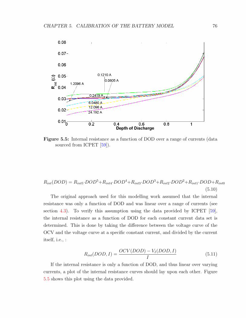
CHAPTER 5. CALIBRATION OF THE BATTERY MODEL 76
Figure 5.5: Internal resistance as a function of DOD over a range of currents (datasourced from ICPET [59]).
Rint(DOD) = Rint5·DOD5+Rint4·DOD4+Rint3·DOD3+Rint2·DOD2+Rint1·DOD+Rint0
(5.10)
The original approach used for this modelling work assumed that the internal
resistance was only a function of DOD and was linear over a range of currents (see
section 4.3). To verify this assumption using the data provided by ICPET [59],
the internal resistance as a function of DOD for each constant current data set is
determined. This is done by taking the difference between the voltage curve of the
OCV and the voltage curve at a specific constant current, and divided by the current
itself, i.e., :
Rint(DOD, I) =OCV (DOD)− VI(DOD, I)
I(5.11)
If the internal resistance is only a function of DOD, and thus linear over varying
currents, a plot of the internal resistance curves should lay upon each other. Figure
5.5 shows this plot using the data provided.

CHAPTER 5. CALIBRATION OF THE BATTERY MODEL 77
Figure 5.6: Plot of polynomial fit of original data from ICPET [59], shown asdashed lines, compared with an OCV curve scaled by an internal resistancecurve, shown as “x”s.
From this plot, it seems that the assumption holds quite well, specifically at lower
currents. As the current increases however, the internal resistance does not remain
constant, indicating that the linear assumption does not hold. It is necessary to
choose an internal resistance curve to represent the internal resistance of the cell over
a range of currents.
Two plots are compared in figure 5.6. The plot on the left shows the polynomial
fits to the original data from ICPET [59] compared with a scaled OCV curve using
the 24.192 A internal resistance curve. The plot on the right shows the polynomial
fits to the original data from ICPET [59] compared with a scaled OCV curve using
the 12.096 A internal resistance curve. Both fits seem to represent the low current
values reasonably. This is because regardless of the subtle changes in internal resis-
tance, when multiplied by small currents they become negligible. The plot on the left
obviously fits the 24.192 A data well, but not so much the other high currents. The
plot on the right fits the high currents quite well, obviously the 12.096 A the best,
however, it does not fit the 24.192 A curve well. This implies that internal resistance
is a function of DOD and current, varying due to changes at the electrochemical level,
and that the modelling assumptions made in section 4.3 are not valid.
To compensate for the change in internal resistance at high currents, an additional

CHAPTER 5. CALIBRATION OF THE BATTERY MODEL 78
Symbol Value if below 16 A Value if above or equal to 16 A
R5 0.1152 0.1972
R4 -0.2556 -0.4749
R3 0.2007 0.4118
R2 -0.0651 -0.1472
R1 0.0265 0.0380
R0 0.0202 0.0154
Table 5.2: Internal resistance coefficients used for the model calibration.
set of internal resistance parameters have been included in the model. They are listed
as parameters 74 to 79 in Appendix B, and are a second set of internal resistance
coefficients to be used in the case of high discrepancies in internal resistance between
discharge curves. Parameter 80 is a current value. If invoked, the model will use
the original internal resistance coefficients (parameters 24-29) for battery currents
less than the current specified in parameter 80, and use the second set of coefficients
(parameters 74-79) for higher battery currents. If the user chooses to only use one
set of coefficients, they need to enter a value of (999.) as any value for parameters 74
to 80, and the model will not make use of them. In which case only the original set
will be used.
Table 5.2 shows the coefficients used in this work. The current limit chosen, i.e.,
parameter 80, is 16 A. In other words, if the current imposed is less than 16 A, the
model will use the first column of coefficients to calculate internal resistance, entered
as parameters 24-29; otherwise, it will use the second column for higher currents
(parameters 74-79).
Parameters 30 to 45 in Appendix B are used to adjust the reference capacity of
the battery to account for changing current, using the α factors discussed in section
4.3 (see eq. 4.8). The model was developed to accept eight different discharge/charge
curves at eight different currents. For each current specified, there should be an
accompanying α factor. In other words, the lowest discharge current will be entered
as parameter 30 and its α factor will be 31, then the next current will be entered as
parameter 32 and its α factor will be 33, etc.

CHAPTER 5. CALIBRATION OF THE BATTERY MODEL 79
Figure 5.7: Voltage as a function of DOD over a range of currents.
To obtain these values, a plot must be made of the cell voltage as a function of
DOD for all the curves similar to figure 5.7. This plot should be limited in the y-axis
range to the lower cutoff voltage, in this work, 3.15 V . The α factors can be found
by measuring the difference in cell capacity relative to the OCV curve as discussed in
section 4.3 (see fig. 4.6).
Table 5.3 shows the α factors used in the model calibration for this work. These
factors will be used and the model will linearly interpolate between them to size the
cell capacity for a varying imposed current. It should be noted that there were only
seven discharge sets provided by ICPET [59], although the model requests eight. In
this case, the user needs to input a value of (999.) as the parameter to describe
the unavailable current, and keep the same α value used for the the previously given
current, to override this last curve. A different user wishing to calibrate a new cell,
can then have as few discharge sets of data, at the sake of losing accuracy, or as many
as eight.
Similar transformations performed to the OCV curve are done to account for
temperature. These temperature variations are applied to the model using parameters

CHAPTER 5. CALIBRATION OF THE BATTERY MODEL 80
Current (A) α
0.0605 1.00
0.1210 1.00
0.2419 1.00
1.2096 0.985
6.0480 0.895
12.096 0.775
24.192 0.593
Table 5.3: Internal resistance coefficients used for model calibration.
46 to 69 in Appendix B. The model allots for eight different temperature curves, and
as discussed in section 4.3, requires that for each temperature, in oC, a β factor (see
eq. 4.10) and a ∆V (T ) drop in voltage value (see eq. 4.9) be declared. In other
words, the lowest temperature will be entered as parameter 46, its β factor will be 47
and its ∆V (T ) will be 48. The next temperature will be entered as parameter 49, its
β factor will be 50 and its ∆V (T ) will be 51, etc.
The original discharge curves for varying temperature data provided from ICPET
[59] were performed at a current density of 7 A·m−2. This was because the simulation
time to run at 0.01 A ·m−2 would have been too long. Thus, to shift the provided
data to simulate OCV curves at various temperatures, the internal resistance effects
due to current had to be removed:
OCV (T, DOD) = V (T, DOD) + I ·Rint (5.12)
where OCV (T, DOD) is the OCV curve at a given temperature T , V (T, DOD) is
the original cell voltage provided, and I ·Rint is the internal resistance due to current
multiplied by the current itself, or in this case 1.2096 A (7 A ·m−2).
Assuming that these curves represent the true OCV curves at these temperatures,
it is now possible to measure the difference in voltage, as temperature changes, with
respect to the 25oC reference curve. This plot is shown below for each temperature
curve as figure 5.8.
From this figure, each voltage curve seems to have a reasonable constant voltage

CHAPTER 5. CALIBRATION OF THE BATTERY MODEL 81
Figure 5.8: Change in voltage as a function of DOD due to cell temperature withrespect to the 25oC reference curve.
difference, with the exception of the -40oC case. In all the other cases, the change
in temperature does not seem to affect voltage with respect to DOD. At extremely
low temperatures however, the cell voltage is adversely affected with respect to DOD
due to changes in the electrochemistry of the cell. Consequently, the average voltage
drop over the entire DOD was taken, and it is assumed that this applied to the -40oC
case. Although this may not be accurate, it is assumed sufficient to model actual cell
behaviour in rare occurrences when the battery would be at those temperatures.
The β factors for temperature are found in the same way as the α factors, relating
to current above. Figure 5.9 shows the temperature curves limited to the cutoff
voltage of 3.15 V , in order to determine the β factors. Table 5.4 shows the average
voltage drop, ∆V (T ), and the β factor, for each temperature. The model will linearly
interpolate between these values to determine a suitable ∆V (T ) and β, for a given
cell temperature.
This chapter discussed all the parameters necessary to calibrate the li-ion model
developed in this work. Its default calibration was performed with simulated data
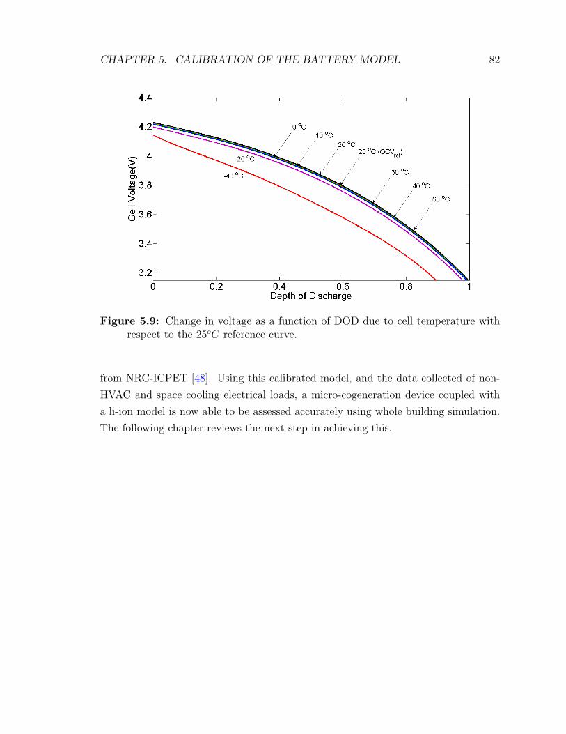
CHAPTER 5. CALIBRATION OF THE BATTERY MODEL 82
Figure 5.9: Change in voltage as a function of DOD due to cell temperature withrespect to the 25oC reference curve.
from NRC-ICPET [48]. Using this calibrated model, and the data collected of non-
HVAC and space cooling electrical loads, a micro-cogeneration device coupled with
a li-ion model is now able to be assessed accurately using whole building simulation.
The following chapter reviews the next step in achieving this.

CHAPTER 5. CALIBRATION OF THE BATTERY MODEL 83
Temperature(oC) ∆V (T )(V ) β
-40 0.1870 0.905
-20 0.0366 0.985
0 0.0123 1.00
10 0.0062 1.00
20 0.0024 1.00
30 -1.4449 ×10⁻⁵ 1.00
40 -0.0012 1.00
60 -0.0012 1.00
Table 5.4: ∆V (T ) values to calibrate li-ion battery model.
Chapter 6
Demonstration of new modelling
capabilities
Chapter 3 reviewed the collection and analysis of Canadian residential non-HVAC
and space cooling electric data. Chapters 4 and 5 reviewed the development and
calibration a li-ion battery model in ESP-r. With the completion of these research
objectives, this chapter demonstrates the new modelling capabilities developed in this
work.
6.1 Li-ion battery model debugging
Inaccuracies in a model can take on many forms, preventing it from exhibiting the
true characteristics of its physical counterpart. These errors can range from misin-
terpretation or simplification of the physical phenomena in the modelling approach,
to errors in the code used to represent the model. Regarding the former of these
errors, they have been continuously addressed throughout sections 4 and 5. Many
simplifications and assumptions have been made throughout the development of the
li-ion model, such as the lumped capacitance approach and the treatment of the heat
transfer process. The validity of these assumptions have been individually addressed
in an effort to simplify the complexity of the physics of a battery, while obtaining a
model with the necessary resolution for use in building simulation.
Finding syntax errors in the source code is a lengthy and ongoing process known
as debugging. Using a pragmatic approach, the six basic battery operating modes
were verified for functionality. These operating modes were normal battery charge
and discharge, over battery charge and discharge, and over battery temperature and
84
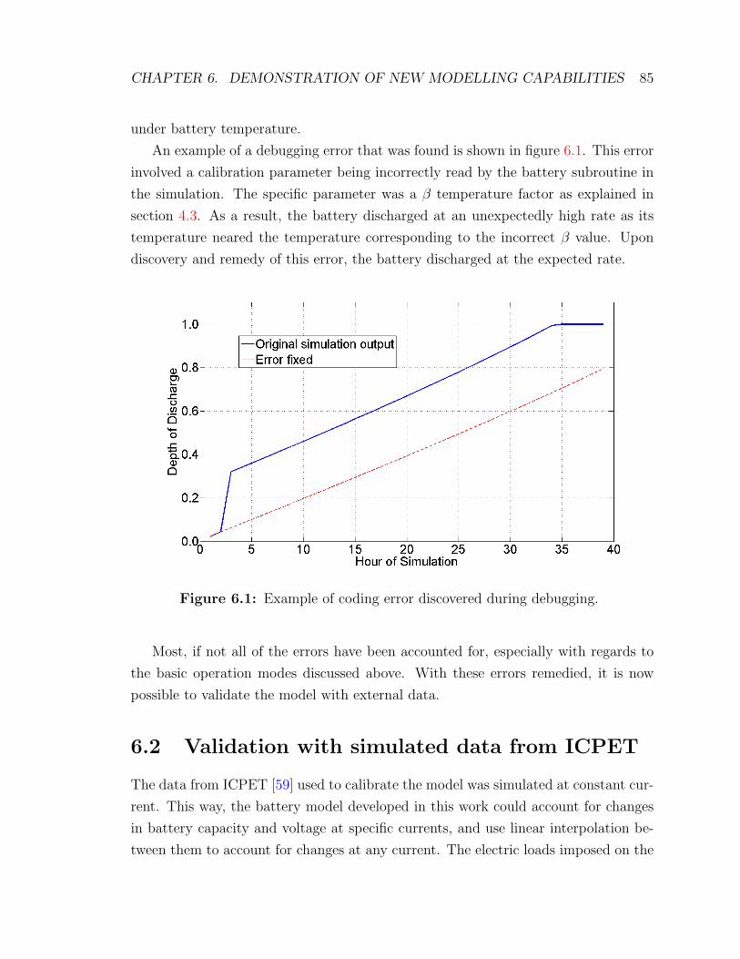
CHAPTER 6. DEMONSTRATION OF NEW MODELLING CAPABILITIES 85
under battery temperature.
An example of a debugging error that was found is shown in figure 6.1. This error
involved a calibration parameter being incorrectly read by the battery subroutine in
the simulation. The specific parameter was a β temperature factor as explained in
section 4.3. As a result, the battery discharged at an unexpectedly high rate as its
temperature neared the temperature corresponding to the incorrect β value. Upon
discovery and remedy of this error, the battery discharged at the expected rate.
Figure 6.1: Example of coding error discovered during debugging.
Most, if not all of the errors have been accounted for, especially with regards to
the basic operation modes discussed above. With these errors remedied, it is now
possible to validate the model with external data.
6.2 Validation with simulated data from ICPET
The data from ICPET [59] used to calibrate the model was simulated at constant cur-
rent. This way, the battery model developed in this work could account for changes
in battery capacity and voltage at specific currents, and use linear interpolation be-
tween them to account for changes at any current. The electric loads imposed on the

CHAPTER 6. DEMONSTRATION OF NEW MODELLING CAPABILITIES 86
battery in ESP-r, however, are specified as a constant power draw over the time-step.
To validate the model developed in this work, a new simulation was requested of
ICPET for a cell discharging at constant power. The new simulation was a cell at
25oC, discharging at a rate of 4.3 W . The li-ion model developed in this work was
modified to be a single cell with the same fixed temperature and the same imposed
electric load. The results are shown in figure 6.2
Figure 6.2: Comparison of li-ion simulation run in ESP-r with simulated data fromICPET [48].
It appears from this figure that the current calculated by ESP-r is lower than the
simulated data from ICPET [48]. This discrepancy could be due to the sensitivity
of the time-step chosen in ESP-r. In ESP-r, the current that the battery charges or
discharges at cannot change within a time-step. However, because the electric load
imposed on the battery over a time-step in ESP-r is constant, the current should
vary because the voltage should vary. Because the voltage does not change within a
time-step either, the subroutine in ESP-r uses an average voltage over the time-step
based on the initial DOD and the predicted final DOD. The current calculated for
the time-step is based on this average voltage.
This indicates that the longer the chosen time-step in a simulation is, the lower the

CHAPTER 6. DEMONSTRATION OF NEW MODELLING CAPABILITIES 87
average voltage is in a discharge scenario and vice versa in a charge scenario. Thus,
for a longer time-step, the current will be lower in discharge and higher in charge.
This is illustrated in figure 6.3. In this figure, the same simulation was performed
with a discharging cell, but with increasing time-steps.
Figure 6.3: Comparison of same simulation in ESP-r with different time-steps toillustrate sensitivity.
As the battery approaches a DOD of one, the BMS reduces the current to zero,
reducing the battery load to zero Watts to prevent over discharging. The time-step
sensitivity is most apparent when the battery load changes. The 60 minute time-step
simulation in figure 6.3 seems illogical because it has no current value below a DOD
of around 0.75. This is because its first current solved was after the first hour of the
simulation, and by this time the cell had already discharged to this DOD. It appears
that an acceptable time-step resolution would be between one and five minutes. If
the battery load varies significantly, a time-step resolution closer to one minute may
be necessary.
Returning to the initial comparison with ICPET, shown in figure 6.2, the voltage
curves compare reasonably as well. There is, however, a consistently lower voltage
in the data from ICPET. The discrepancy of around 0.01 V can be attributed to a

CHAPTER 6. DEMONSTRATION OF NEW MODELLING CAPABILITIES 88
consistently higher current in the ICPET data, resulting in a higher internal resis-
tance, and a larger voltage drop away from the OCV. With the model performing as
expected, when compared with data from ICPET [48], it can now be integrated with
a cogeneration device to simulate satisfying the electrical and thermal demands of a
household.
6.3 Demonstration of integrated system
6.3.1 ESP-r model description
To demonstrate the capability of the li-ion model developed in this work, a model of
a house was created in ESP-r for an annual simulation. The geometry of the house
was basic: a single-zone, rectangular house located in Ottawa, ON. The model used
typical constructions to represent the house’s walls, ceiling and floor. It had a floor
space of 132 m2 and a volume of 528 m3. These values were chosen to be close to
those in a typical Canadian single family detached dwelling [2]. Because the objective
here was to observe the functionality of a RES plant system using accurate household
electricity usage data (elaborated further), emphasis was not placed on the detail
of the house’s geometry. A weather file of Ottawa, ON from 2008, collected from
Environment Canada’s Weather Office [5], was used for the simulation.
A schematic of the plant configuration used in the simulation is shown in figure 6.4.
A SE model, developed by Ferguson [61] for IEA/ECBCS’s Annex 42 [1], was used
as the cogeneration device in the simulation. The SE was configured to constantly
produce 900 W of electricity for the house throughout the year. The engine had a
constant electrical efficiency of 9.29%, and a constant thermal efficiency of 90.71%.
Some of the recovered heat was lost to the SE’s surroundings as described by Ferguson
[61]. For this example, the engine was placed outside of the house, exposed to ambient
temperatures.
The useful heat recovered by the engine was circulated via a pump to an air-to-
water heat exchanger. The air-to-water heat exchanger, driven by a fan, supplied
warm air to the household. The pump and the fan consumed 50 W and 25 W of
electricity, each, in the simulation. Refer to figure 6.4 for this schematic.
The electric household demands were input as combined non-HVAC and space
cooling demands on a five minute basis. One of the medium energy houses from the

CHAPTER 6. DEMONSTRATION OF NEW MODELLING CAPABILITIES 89
Figure 6.4: Plant system schematic for application demonstration.
data collection project, labelled H6 in section 3, was used for these demands. A SE in
reality produces DC power and the battery stores DC power. A power conditioning
unit (PCU) would traditionally transform this power to AC before sending it to the
house. Because the data collected in the measurement project from this work (see
section 3) recorded real power, i.e., DC, after taking into account the power factor,
there is no need to condition the DC power to AC. Essentially, it is similar to having
a PCU unit between the battery and the house with an assumed efficiency of 100%.
While this assumption may not be accurate in reality, it is sufficient to demonstrate
this work’s new modelling capabilities.
A control law needs to be implemented to dictate the function of each device
in the plant system on how they will satisfy the household’s energy demands. For
this example, a simple control law was implemented to treat the house’s electric and
thermal demands. If the combined electricity demand from the household, pump and
fan exceeded the 900 W produced by the SE, the battery would discharge, within safe
limits, to meet the excess. If the combined electricity demand from the household,
pump and fan was less than the SE’s production, the battery would charge with
the excess electricity produced. If the SE and battery could not meet the combined
electric demand, electricity would be imported from the grid. Likewise, if the SE’s
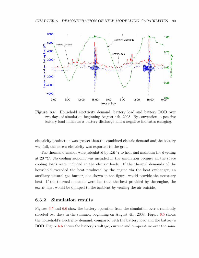
CHAPTER 6. DEMONSTRATION OF NEW MODELLING CAPABILITIES 90
Figure 6.5: Household electricity demand, battery load and battery DOD overtwo days of simulation beginning August 4th, 2008. By convention, a positivebattery load indicates a battery discharge and a negative indicates charging.
electricity production was greater than the combined electric demand and the battery
was full, the excess electricity was exported to the grid.
The thermal demands were calculated by ESP-r to heat and maintain the dwelling
at 20 oC. No cooling setpoint was included in the simulation because all the space
cooling loads were included in the electric loads. If the thermal demands of the
household exceeded the heat produced by the engine via the heat exchanger, an
auxiliary natural gas burner, not shown in the figure, would provide the necessary
heat. If the thermal demands were less than the heat provided by the engine, the
excess heat would be dumped to the ambient by venting the air outside.
6.3.2 Simulation results
Figures 6.5 and 6.6 show the battery operation from the simulation over a randomly
selected two days in the summer, beginning on August 4th, 2008. Figure 6.5 shows
the household’s electricity demand, compared with the battery load and the battery’s
DOD. Figure 6.6 shows the battery’s voltage, current and temperature over the same

CHAPTER 6. DEMONSTRATION OF NEW MODELLING CAPABILITIES 91
time frame.
Figure 6.6: Battery voltage, current and temperature over two days of simulationbeginning August 4th, 2008. By convention, a positive current indicates abattery discharge and a negative indicates charging.
By convention in these figures, a positive power and current value indicated that
the battery was discharging while a negative value indicated charging. Over the
nighttime of both days, the electric demand of the household was less than the pro-
duction of the SE (see fig. 6.5). During these periods, the SE was able to satisfy the
household demand and charge the battery with its excess electricity production. Over
the daytime, the household electricity demand increased above the production of the
SE and the battery began to discharge to satisfy it. Towards 18:00 on both days,
the battery discharged too far while the demand was still too high. Here, electricity
had to be imported from the grid to satisfy the demand. As the household activity
dropped below the production of the SE in both evenings, the battery charged with
the SE’s excess electricity production.
The battery voltage, current and temperature seem to perform as expected (see
fig. 6.6). As the battery discharged too far, it needed to charge itself back into a safe
operating range. This is the reason for the rapid fluctuations in current at 18:00 on

CHAPTER 6. DEMONSTRATION OF NEW MODELLING CAPABILITIES 92
Discharge Current (A) Charge Current (A) Temperature oC
Mean 4.67 3.56 20.75
St. Dev 7.79 3.75 1.80
Max. 101.8 101.8 60.66
Min. 0 0 20.00
Table 6.1: Current and temperature statistics for annual simulation.
both days; the battery tried to meet the household demand, while the BMS tried to
keep the battery in safe limits. This resulted in charging and discharging currents
as high as 63 A. The internal resistance resulting from the high current caused the
battery temperature to rise from 20 oC to 34.8 oC (on the first day). The fluctuations
of current at 18:00 on both days represents a flaw in the overall control strategy of
the HVAC system. These current fluctuations would result in a loss of energy due
to high internal resistances and would inflict damage on the battery. With a more
sophisticated control on the HVAC system, these fluctuations could be avoided. This
HVAC control strategy will be discussed in the future work section.
Table 6.1 lists information about the battery’s charge current, discharge current
and temperature over the entire year. It provides their means, standard deviations,
maximum and minimum values. Using the battery degradation model developed in
this work (see sect. 5.2.1), the battery used approximately 798 cycles over the year.
This would equate to a lifespan of 3.76 years for a 3000 cycle battery life. If the
long-term industry goal of a 10,000 cycle life span can be realized [62] this would
equate to a lifetime of more than 12 years.
The values of table 6.1 show that the battery model behaves as expected over
the entire simulation. Both discharge and charge currents have the same maximum
value. These were for an empty battery or a full battery trying to charge or discharge
at the maximum possible rate, respectively. The mean and standard deviation show
higher values in discharge than in charge. This would seem appropriate because the
charge was coming from a constant steady rate, when the house loads were low with
no appliances. Whereas, the discharge was dictated by the highly varying household
demand from appliances and space cooling. The battery temperature stayed close to
the controlled temperature of the zone, shown by the mean and standard deviation.

CHAPTER 6. DEMONSTRATION OF NEW MODELLING CAPABILITIES 93
In periods of high charge and discharge, the temperature reached values greater than
60 oC before the BMS prevented further heating.
Another annual simulation was performed for comparison. This simulation was
identical to the previous, except that the battery was removed from the plant system.
Figures 6.7 and 6.8 shows the comparison of these two simulations.
Figure 6.7: Total monthly heat dump from the SE to the ambient surroundings.
Figure 6.7 shows the monthly heat dumped by the SE, equal in both simulation
scenarios. The heat generated by the SE was ample all year around to meet the
thermal demands of the dwelling, and no auxiliary burner was required. This would
indicate that this system was oversized in a thermal sense to meet the household
demands. Note, however, that the thermal demands of the household were not the
emphasis of this example. Proper treatment of infiltration with the exterior, windows
and DHW considerations would change these results.
Figure 6.8 compares the total grid imports and exports of electricity on a monthly
basis between the two scenarios. This figure shows that the coupling of a li-ion battery
to a SE cogeneration device improved the performance of the system by reducing the
grid interaction. In every month, the amount of electricity either imported from the

CHAPTER 6. DEMONSTRATION OF NEW MODELLING CAPABILITIES 94
Figure 6.8: Simulation comparison with and without use of li-ion battery. The totalmonthly electric grid imports and exports are shown for both scenarios.
grid, or exported to the grid, was reduced. In general, the amount of electricity
exported to the grid exceeded the amount of electricity imported. Once again this,
indicates that the SE was oversized in this example.
The control law implemented in this example was quite simple; the battery acted
essentially as a buffer between the electric demands of the household and the gener-
ation by the SE. More sophisticated controllers could significantly improve the per-
formance of this system and reduce grid interaction further. The optimization of a
custom controller developed for a RES system is complex, yet crucial to assess its full
potential. The implementation of such a controller and a full assessment of a RES
system are beyond the scope of this work. The future work section will elaborate on
this further.
This chapter covered the testing and validation of the calibrated li-ion battery
model developed in this work. It also demonstrated the new modelling capabilities of
the li-ion model coupled with a SE using the residential electric usage data collected in
this work. With this, an entire RES system model is ready to be optimally controlled
and assessed to reduce household electricity consumption and peak demand.

Chapter 7
Conclusions & Future Work
7.1 Conclusions
Peak electricity demand in residential dwellings is a significant contributor of GHG
emissions and inefficient electricity production. Preliminary assessments of micro-
cogeneration devices, as a solution to peak power demand, recommended that electric
storage may improve their ability to meet highly varying residential electric demand.
Certain gaps existed to accurately assess a micro-cogeneration device coupled with
battery storage using building simulation. Addressing these gaps were the objectives
of this research.
One objective of this research was to gain a better understanding of residential
electricity usage at a fine time resolution to improve the validity of building simula-
tions. Non-HVAC and space cooling electricity usage of twelve homes in the Ottawa,
Ontario area were gathered at one-minute intervals for a study period of one year
beginning in the summer of 2009.
The analysis of the non-HVAC data collected in the project showed that electricity
usage varied significantly between households. The results showed that averaging
data over a large number of days eliminated many of the peaks that occurred in the
household, and was not a good method of analyzing peak power demand. Histograms,
however, were able to show the distribution of electric draws, over many days, while
still retaining the largest occurrences of electric draws. The analysis also showed,
when compared to synthetically generated profiles, that residential electric loads may
be too complex to capture in algorithms used for profile generation. A new technique,
discussed in the future work section below, may offer a new approach in generating
95

CHAPTER 7. CONCLUSIONS & FUTURE WORK 96
profiles. The data collected provides excellent simulation inputs for representing non-
HVAC electricity use of Canadian households in building simulation.
The analysis of the space cooling data gathered in the project showed that air-
conditioning consumption varied between households. This was not only in total
electricity consumed, but at what time of day as well. A scatter plot of the daily air-
conditioning electricity consumption with the maximum daily temperature and mean
daily temperature showed a strong relationship that also varied between households.
The data collected provides excellent validation of new algorithms in building simu-
lation to capture the complexities of occupant habits with respect to space cooling;
this is elaborated in the future work section below.
Another objective of this research was to develop a li-ion battery model and couple
it with an existing cogeneration device in ESP-r. The model developed, based on an
approach by Gao et al. [50], is able to account for variations in imposed current and
battery temperature on performance. The model functionality includes long-term
degradation, self-discharge, and thermal interaction with its surroundings, and can
be sized to different capacities depending on its application.
Default calibration of the model was done with simulated data from NRC-ICPET
[59] in chapter 5. The data provided was the cell voltage and DOD relationship
of a simulated cell at different currents and temperatures. The model developed in
this work was calibrated for a 6 kW · h battery with a nominal voltage of 120 V ,
using the data from ICPET and other data found in the literature review. Chapter 5
also explained the steps in calibrating different li-ion chemistries to the model. The
model was validated with a different data set of a cell discharging at constant power,
provided by ICPET, as well.
The new modelling capabilities, developed in this work, was demonstrated in
Chapter 6. This was an annual simulation of the thermal and electric demands of a
household being satisfied by a SE coupled with a li-ion battery. The electricity use
data gathered in this work was used for the household’s electric demands. While the
example was quite simple in control, the implementation of electric storage saw the
reduction of grid interaction with the house in every month. The model behaved as
expected, consuming 27% of its useable life over the year, according to the battery
degradation model implemented. The battery management system (BMS) kept the
battery in safe charging and temperature ranges. The implementation of a custom
optimized controller on the entire plant system would improve performance. This is

CHAPTER 7. CONCLUSIONS & FUTURE WORK 97
discussed in the future work section below.
The objectives that were set out in this research have been successfully met. Rec-
ommendations for future work in this area is discussed below. With a full assessment
of the potential of li-ion storage, coupled with micro-cogeneration, residential peak
electricity demand and GHG emissions may be significantly reduced.
7.2 Future Work: Non-HVAC and space cooling
Residential non-HVAC electricity future work
Chapter 3 reviewed the electric measurement project, performed in this work, of
Canadian houses. It showed the analysis of non-HVAC and space cooling electricity
usage of twelve houses, in the Ottawa, ON area, at one minute intervals over one
year.
As discussed in the literature review of non-HVAC electricity use (see section
3.1), similar projects aimed at producing randomly generated non-HVAC profiles,
for use in building simulation, tend to use the data collected to develop algorithms.
These algorithms are then used to produce new profiles. However, as seen in the
results from this work on non-HVAC electricity use (see section 3.3), these algorithms
generalize occupant activities into routines, and lack the complexity to truly represent
the occupants’ constantly changing lives.
To represent the stock of Canadian households with randomly generated profiles,
a new technique discussed by Hill [63] may provide an interesting approach. This
technique would use empirically measured data, similar to the work done in this
research, to statistically analyze the distribution of electricity use. The analysis would
be for not only means and variances, but also the correlations factors with respect to
future time-steps, known as autocorrelation. An autocorrelation factor (ACF) reflects
the relationship between a variable, x, at a present time-step, and the same variable
k time-steps later. The value k is known as the lag.
ACF =
∑n−ki=1 (xi − x)(xi+k − x)∑n
i=1(xi − x)2(7.1)
An ACF of one, for a given time-step and lag k, indicates a strong relationship
between the variable at this time-step, and the variable at k time-steps later. A value
of negative one indicates a strong inverse relationship, and a value of zero indicates
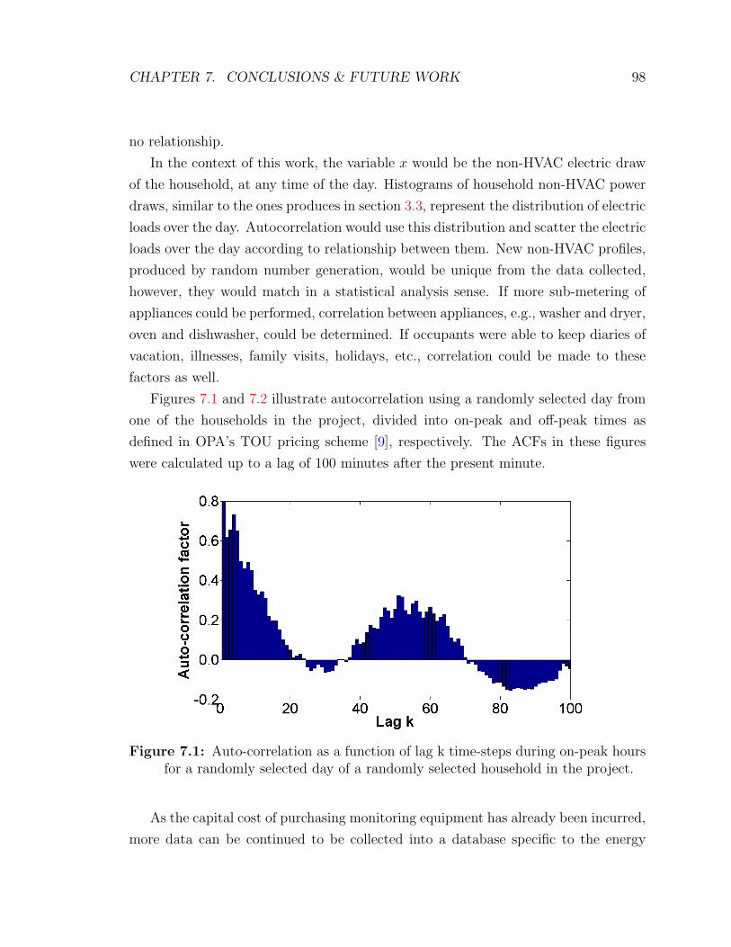
CHAPTER 7. CONCLUSIONS & FUTURE WORK 98
no relationship.
In the context of this work, the variable x would be the non-HVAC electric draw
of the household, at any time of the day. Histograms of household non-HVAC power
draws, similar to the ones produces in section 3.3, represent the distribution of electric
loads over the day. Autocorrelation would use this distribution and scatter the electric
loads over the day according to relationship between them. New non-HVAC profiles,
produced by random number generation, would be unique from the data collected,
however, they would match in a statistical analysis sense. If more sub-metering of
appliances could be performed, correlation between appliances, e.g., washer and dryer,
oven and dishwasher, could be determined. If occupants were able to keep diaries of
vacation, illnesses, family visits, holidays, etc., correlation could be made to these
factors as well.
Figures 7.1 and 7.2 illustrate autocorrelation using a randomly selected day from
one of the households in the project, divided into on-peak and off-peak times as
defined in OPA’s TOU pricing scheme [9], respectively. The ACFs in these figures
were calculated up to a lag of 100 minutes after the present minute.
Figure 7.1: Auto-correlation as a function of lag k time-steps during on-peak hoursfor a randomly selected day of a randomly selected household in the project.
As the capital cost of purchasing monitoring equipment has already been incurred,
more data can be continued to be collected into a database specific to the energy

CHAPTER 7. CONCLUSIONS & FUTURE WORK 99
Figure 7.2: Auto-correlation as a function of lag k timesteps during off-peak hoursfor a randomly selected day of a randomly selected household in the project.
consumption, location, size, number of occupants, etc. This database could be used to
generate random statistically significant electricity use profiles of a specific household,
if desired, or general profiles based on the entire database.
New strategies such as DSM, storage and micro-cogeneration could be simulated
with the general database, with sensitivity analysis on specific houses, to observe the
potential in specific cases. If the database could be randomly selected without bias,
new strategy potentials could not only be assessed, but at what level of penetration
they could occur. This could have residual effects on pricing schemes and costs of
implementation.
Residential space cooling electricity future work
The space cooling data collected in this work provided excellent information on
air-conditioning usage of Canadian houses. It was shown, in section 3.4, that air-
conditioning usage varied significantly between households. This can be attributed
to several factors, as discussed, including window openings and shading.
A simulation of cooling loads, using only a temperature set-point to control air-
conditioning usage, would typically show different space cooling usage than the data
collected in this work. This is because of occupant intervention in reality. Beausoleil-
Morrison’s [30] work on implementing opening and shading algorithms in building

CHAPTER 7. CONCLUSIONS & FUTURE WORK 100
simulation tries to realistically predict space cooling usage by simulating an occupant’s
intervention to mitigate it. With the information gathered in the survey that the
occupants in the project filled out on openings, shading and their thermostat set-
points, new algorithms using random number generation can be implemented. These
would based on the probabilities of occupant intervention with openings and shading.
These algorithms could also incorporate more sophisticated thermostat control set-
points, in an effort to match the data collected in this project. New work in this area
can use the space cooling usage data collected in this research for validation of these
algorithms.
7.3 Future Work: Li-ion battery model
Calibration of model with an actual cell
The li-ion battery model developed in this work provides a novel method of incorpo-
rating an electric storage device in the building simulation tool ESP-r. The next step
in this work is the calibration of the model with a commercially available li-ion cell.
This would include charge and discharge curves of the cell at various constant currents
and temperatures. This calibration would provide extensive validation in the mod-
elling approaches used in this work, and provide new information of the complexities
of real cells.
Verification and improvements to the li-ion model
Specific aspects of the li-ion model may need to be revisited, namely: the assump-
tions made in the heat transfer between the battery and its environment, battery
degradation treatment, self-discharge parameters and parasitic power draws of the
BMS. The realistic treatment of cell balancing in a battery would also need accurate
treatment in the future. This could involve research into typical ways that cells be-
come imbalanced in a battery pack. The implementation in the BMS of individual
cell voltage monitoring and in the case of imbalances, discharging to keep the battery
pack balanced, would approach a more realistic model.

CHAPTER 7. CONCLUSIONS & FUTURE WORK 101
RES control future work
As discussed, the control of a plant system dictates the function of each component
within, and is the most important factor in its performance. Simple controls of single-
component plant systems occur in a general way:
• Sense - A property is sensed in the model. This can be any property e.g.,
temperature, relative humidity, flow rates of plant systems and household energy
demand.
• Control law - A control law is implemented to meet the sensed property. This
can be as simple as an on/off switch control, or towards more sophisticated
controllers such as proportional, differential, integrated (PID) controllers.
• Actuate - The device under the control law is actuated. This can be anything
from the opening of valves, to increases of flow rates, to diversions of electricity
flows like in the context of this work.
While these steps have been implemented in ESP-r and work well for single com-
ponent systems, an integrated system with many components may require a custom
sophisticated controller. These custom controllers are unique subroutines in the sim-
ulation program that dictate the function of all the components in the plant. Similar
controllers have already been implemented in ESP-r [64].
A controller for RES should consider the energy sources and sinks of the model.
In a thermal context, the sources are the cogeneration device and the sinks are the
thermal demands of the house and DHW. In an electrical context, the sources are
the cogeneration device and the sinks are the house’s non-HVAC and space cooling
electrical loads.
The storage device may act as a source or a sink. In an electrical context, this is
the li-ion battery. Even in a thermal context, a hot water tank may be introduced
for storage to improve performance.
A custom controller for RES could exist on many levels of resolution. The lowest
level of controllers can involve the constant operation of the cogeneration device with
the storage devices acting as buffers between the production and the demand. This
is similar to the control implemented in the demonstration in section 6.3.
The next level of controller would involve either thermal load following or electric
load following. In other words, the function of the cogeneration device would depend

CHAPTER 7. CONCLUSIONS & FUTURE WORK 102
on either the household electric demand, or the household thermal demand. In this
case, barring transient effects, the storage devices would be most effective at satisfying
the demand of the load that is not being followed. In other words, a battery would
be most effective in a thermal load following scenario, and a hot water storage tank
would be most effective in an electric load following scenario.
Intermediate levels of controllers would involve assessing the state of energy of the
storage devices for the operation of the cogeneration device. In other words, if the
battery’s SOC or the storage tank’s temperature is too low, the cogeneration device
would turn on. The cogeneration device would turn off once the battery’s SOC or
storage tank temperature reached a high value. This, however, still neglects transient
warm up times of the cogeneration device. The control developed by Beausoleil-
Morrison et al. [64] works in this fashion.
High level controllers incorporate a broad range of definitions and can quickly
become complicated. They can include consideration for transient operation, TOU
pricing schemes, fuel and electricity costs, present household energy demand, and
with the advantage of building simulation and weather forecasting, future household
energy demand.
It is necessary to determine which parameter is being optimized in a high level
controller. This could be GHG emissions, utility cost (to the user and/or to the
utility provider), grid interaction minimization, or peak demand reduction, to name
a few. These parameters are not necessarily mutually exclusive, and significant work
should be done in this area to determine which parameter to maximize for system
optimization.
Figure 7.3 is a brief, general, flow chart of a more sophisticated controller for a
RES system. It attempts to reduce cost of electricity, specifically in peak demand
periods. Because it follows an electric demand, adequate thermal storage would likely
improve the thermal aspect of the system.
The sensing action compares the cost of producing electricity from the cogenera-
tion device, compared to that of purchasing from the grid. This would consider the
electrical efficiency of the device, and maybe the transmission losses from the grid. It
could also consider the thermal demands of the house, and the cost of producing aux-
iliary heat. In this way, the device can include its thermal efficiency as an incentive to
produce onsite. Another sensing option shown in figure 7.3 is to use the household’s
electric demand to govern the function of the system. This critical value can be the

CHAPTER 7. CONCLUSIONS & FUTURE WORK 103
baseload, in an effort to reduce peak demand, or any demand, if the system is to meet
all the household electric loads. The remainder of the control dictates the interaction
between the power produced by the cogeneration device and the battery’s SOC. The
controller aims to use the battery as a buffer between the cogeneration device and the
household in transient warm-up times, while the device’s off-performance efficiency
is poor.
This is just an example of the future work necessary in the control of a RES system.
The next step, after an accurate assessment of a RES system being controlled in an
optimized manner, would be the development of a battery prototype. This prototype
would be based on the size and parameters recommended by the assessment. If
feasible from the assessment, the prototype would provide the framework for the
implementation of a li-ion battery coupled with a cogeneration device in residential
households to reduce peak residential electricity demand.

CHAPTER 7. CONCLUSIONS & FUTURE WORK 104
Actuate Turn off cogen (if on), use grid
electricity for demand and proceed to next time step
Keep battery charged: SOCbatt > SOChigh
Actuate Turn on cogen (if off) and assess its electric output
(Pcogen)elec
Yes
Yes Is (Pcogen)elec < (PHouseDemand)elec
and (SOCbatt)t+Δt < SOClow
(PHouseDemand)elec = (Pcogen)elec + Pbatt + Pgrid
(PHouseDemand)elec = (Pcogen)elec
Charge battery: Pbatt = (Pcogen)elec –
(PHouseDemand)elec (PHouseDemand)elec = (Pcogen)elec –
Pbatt
Is (Pcogen)elec > (PHouseDemand)elec Yes
Next timestep
No
Sensor criteria Is ($/kWh)cogen ≤($/kWh)grid
or (PHouseDemand)elec > critical
No
No
Is (Pcogen)elec = (PHouseDemand)elec Yes
Begin timestep
Figure 7.3: Example of custom controller flowchart for RES.

References
[1] I. Beausoleil-Morrison, ed., An Experimental and Simulation-Based Investigation
of the Performance of Small-Scale Fuel Cell and Combustion-Based Cogeneration
Devices Serving Residential Buildings. IEA/ECBCS Annex 42 Report, 2008.
[2] “Energy use data handbook 1990 to 2007,” tech. rep.,
Natural Resources Canada, 2009. Accessible online at
http://oee.nrcan.gc.ca/publications/statistics/handbook08/index.cfm?attr=0.
[3] “Survey of household energy use 2003,” tech. rep., Office of En-
ergy Efficiency, Natural Resources Canada, 2005. Accessible online at
http://oee.nrcan.gc.ca/Publications/statistics/sheu-summary/index.cfm.
[4] “Factor analysis of ontario electricity use - 1990-2003,” tech. rep., ICF Consult-
ing, Chief Conservation Officer-Ontario Power Authority, 2005.
[5] “Daily data report Ottawa, Ontario,” tech. rep., Evironment Canada: Weather
Office, 2010. Accessible online at http://climate.weatheroffice.gc.ca/.
[6] “Hourly generator output capability and demand for June 7th, 2008,” tech.
rep., Independent Electricity Service Operator, 2009. Accessible online at
http://www.ieso.ca/imoweb/marketdata/genEnergy.asp.
[7] “Electric power generation, transmission and distribution,” tech. rep., Statistics
Canada, 2007. Accessible online at http://www.statcan.gc.ca/.
[8] “Ontario’s integrated power system plan,” tech. rep., Ontario Power Authority,
2007. Accessible online at http://www.powerauthority.on.ca/ipsp/.
[9] “Ontario energy board smart price pilot,” tech. rep., IBM Global Busi-
ness Services and eMeter Strategic Consulting for the Ontario Energy Board,
105

REFERENCES 106
2007. Accessible online at http://www.oeb.gov.on.ca/documents/cases/EB-
2004-0205/smartpricepilot/OSPP0Final
[10] R. Shaw, “The value of reducing distribution losses by domestic load-shifting: a
network perspective,” Energy Policy, vol. 37, no. 8, p. 3159, 2009.
[11] I. Knight and I. Ugursal, “Residential cogeneration systems: A review of the
current technologies,” tech. rep., Subtask A of FC+COGEN-SIM The Simula-
tion of Building-Integrated Fuel Cell and Other Cogenearation Systems. Annex
42 of the International Energy Agency Energy Conservation in Buildings and
Community Systems Programme, 2005.
[12] H. Ibrahim, “Energy storage systems - characteristics and comparisons,” Renew-
able sustainable energy reviews, vol. 12, no. 5, pp. 1221–50, 2008.
[13] I. Hadjipaschalis, “Overview of current and future energy storage technologies
for electric power applications,” Renewable sustainable energy reviews, vol. 13,
no. 6, p. 1513, 2009.
[14] G. Nazri and G. Pistoia, Lithium batteries: science and technology. Boston:
Kluwer Academic Publishers, 2004.
[15] P. G. Bruce, “Energy storage beyond the horizon: Rechargeable lithium batter-
ies,” Solid State Ionics, vol. 179, no. 21, p. 752, 2008.
[16] J. Hassoun, “Recent advances in liquid and polymer lithium-ion batteries,” Jour-
nal of materials chemistry, vol. 17, no. 35, p. 3668, 2007.
[17] G. Hunt, “The great battery search,” IEEE Spectrum, vol. 35, no. 11, pp. 21 –
8, 1998.
[18] J. McDowall, Battery life considerations in energy storage applications and their
effect on life cycle costing. Saft America at Power Engineering Society Summer
Meeting, 2001.
[19] S. McGarry, “Lithium-ion battery life cycle.” email correspondance, Department
of Electronics, Carleton University, Ontario, Canada.
[20] D. Linden and T. B. Reddy, Linden’s handbook of batteries. New York: McGraw-
Hill,, 2001.

REFERENCES 107
[21] H. Ibrahim, “Comparison and analysis of different energy storage techniques
based on their performance index,” 2007 IEEE Canada Electrical Power Con-
ference (EPC ’07), p. 393, 2007.
[22] I. Davidson, “Lithium ion market costs.” email correspondance, Institute for
Chemical Process and Environmental Technology, National Research Council
Canada, 2009.
[23] “USABC goals for advanced batteries for EVs,” tech. rep., United States Council
for Automotive Research LLC, 2009.
[24] D. P. Jenkins, “Model for evaluating impact of battery storage on microgenera-
tion systems in dwellings,” Energy conversion and management, vol. 49, no. 8,
p. 2413, 2008.
[25] Glasgow: University of Strathclyde, The ESP-r system for building energy sim-
ulations: user guide version 9 series, ESRU Manual U00/1, 2000.
[26] H. Ribberink and W. Wang, “Improving ESP-r’s battery model with active bat-
tery life control and coverage of vanadium redox flow batteries,” Proceedings
eSim2008 Conference, 2008.
[27] J. A. Clarke, Energy Simulation in Building Design. Butterworth-Heinemann,
2nd ed., 2001.
[28] I. Knight, N. Kreutzer, M. Manning, M. Swinton, and H. Ribberink, “European
and Canadian non-HVAC electric and dhw load profiles for use in simulating
the performance of residential cogeneration systems,” tech. rep., Subtask A of
FC+COGEN-SIM The Simulation of Building-Integrated Fuel Cell and Other
Cogenearation Systems. Annex 42 of the International Energy Agency Energy
Conservation in Buildings and Community Systems Programme, 2007.
[29] M. Armstrong, M. Swinton, H. Ribberink, I. Beausoleil-Morrison, and J. Millete,
“Synthetically derived profiles for representing occupant-driven electric loads in
Canadian housing,” Journal of Building Performance Simulation, vol. 2, no. 1,
pp. 1–41, 2009.

REFERENCES 108
[30] I. Beausoleil-Morrison, “On predicting the magnitude and temporal variation
of cooling loads in detached residential buildings,” Building Simulation 2009
Conference Proceedings, 2009.
[31] P. A. Strachan, “History and development of validation with the ESP-r simula-
tion program,” Building and Environment, vol. 43, no. 4, p. 601, 2008.
[32] W. Wang, “Evaluation of the Alberta air infiltration model using measurements
and inter-model comparisons,” Building and Environment, vol. 44, no. 2, p. 309,
2009.
[33] B. Lomanowski, “Implementation of window shading models into dynamic whole-
building simulation,” Master’s thesis, University of Waterloo, Waterloo, Ontario,
2008.
[34] N. Kelly, Towards a design environment for building integrated energy systems:
The integration of electrical power flow modelling with building simulation. PhD
thesis, University of Strathclyde, Glasgow, UK, 1998.
[35] J. A. Clarke, “Integrating power flow modelling with building simulation,” En-
ergy and Buildings, vol. 33, no. 4, p. 333, 2001.
[36] N. Isaacs, M. Camilleri, L. French, A. Pollard, K. Savill-Smith, R. Fraser,
P. Rossouw, and J. Jowett, “Energy use in New Zealand households - HEEP
year 10 report,” tech. rep., BRANZ Group, New Zealand, 2006. Accessible on-
line at http://www.branz.co.nz/.
[37] D. Parker, “Research highlights from a large scale residential moni-
toring study in a hot climate, FSEC-PF369-02,” tech. rep., Florida
Solar Energy Center, Cocoa, Florida, 2002. Accessible online at
http://www.fsec.ucf.edu/en/publications/html/FSEC-PF-369-02/.
[38] G. Newsham, “Electrical load study of Ontario households.” email corre-
spondance, Institute for Research in Construction, National Research Council
Canada, 2010.
[39] I. Beausoleil-Morrison, “A model for simulating the thermal and electrical pro-
duction of small-scale solid-oxide fuel cell cogeneration systems within building
simulation programs,” HVAC R Research, vol. 12, no. 3, p. 641, 2006.
REFERENCES 109
[40] J. Widen, M. Lundh, I. Vassileva, E. Dahlquist, K. Ellegard, and E. Wackelgard,
“Constructing load profiles for household electricity and hot water from time-
use data. Modelling approach and validation,” Energy and Buildings, vol. 41,
pp. 753–768, 07 2009.
[41] A. Capasso, W. Grattieri, R. Lamedica, and A. Prudenzi, “A bottom-up ap-
proach to residential load modeling,” Power Systems, IEEE Transactions on,
vol. 9, no. 2, pp. 957–964, 1994.
[42] J. V. Paatero and P. D. Lund, “A model for generating household electricity load
profiles,” International Journal of Energy Research, vol. 30, no. 5, pp. 273–290,
2006.
[43] C. F. Walker and J. L. Pokoski, “Residential load shape modelling based
on customer behavior,” IEEE Transactions on Power Apparatus and Systems,
vol. PAS-104, pp. 1703–1711, 1985 JULY 1985.
[44] G. Gross and F. D. Galiana, “Short-term load forecasting,” Proceedings of the
IEEE, vol. 75, no. 12, pp. 1558–1573, 1986.
[45] H. K. Alfares and M. Nazeeruddin, “Electric load forecasting: literature survey
and classification of methods,” International Journal of Systems Science, vol. 33,
pp. 23 – 34, 2002.
[46] R. Abernethey, R. Benedict, and R. Dowdell, “ASME measurement uncertainty,”
Journal of fluids engineering, vol. 107, pp. 161–164, 1985.
[47] R. Moffat, “Describing the uncertainties in experimental results,” Experimental
Thermal and Fluid Science, vol. 1, no. 1, pp. 3–17, 1988.
[48] K. Darcovich, “Residential electrical power storage scenario simulations with a
large-scale lithium ion battery,” Journal of Applied Electrochemistry, vol. 40,
no. 4, pp. 749–755, 2010.
[49] R. Dell and D. A. J. Rand, Understanding batteries. Cambridge: Royal Society
of Chemistry, 2001.
[50] L. Gao, S. Liu, and R. Dougal, “Dynamic lithium-ion battery model for system
simulation,” IEEE Transactions on Components and Packaging Technologies,
vol. 25, no. 3, pp. 495 – 505, 2002.

REFERENCES 110
[51] “Energizer technical bulletin: Battery internal resistance,” tech.
rep., Energizer Holdings, Inc., 2005. Accessible online at
http://data.energizer.com/PDFs/BatteryIR.pdf.
[52] P. B. Balbuena and Y. Wang, Lithium-ion batteries : solid-electrolyte interphase.
London: Imperial College Press, 2004.
[53] M. W. Verbrugge, “Electrochemical and thermal characterization of battery
modules commensurate with electric vehicle integration,” Journal of the Elec-
trochemical Society, vol. 149, no. 1, p. A45, 2002.
[54] S. Soo, “Factors that affect cycle-life and possible degradation mechanisms of a
Li-ion cell based on LiCoO2,” Journal of Power Sources, vol. 111, no. 1, p. 130,
2002.
[55] R. Spotnitz, “Simulation of capacity fade in lithium-ion batteries,” Journal of
Power Sources, vol. 113, no. 1, pp. 72–80, 2003.
[56] J. P. Holman, Heat tansfer. New York: McGraw-Hill Companies, 1997.
[57] P. Pinel, “Immosolars battery model: Battery and thermal management system,”
tech. rep., Immosolar ABT, Santa Ponsa, Spain, 2006.
[58] B. Y. Liaw, “Modeling of lithium ion cells - a simple equivalent-circuit model
approach,” Solid State Ionics, vol. 175, no. 1, pp. 835–9, 2004.
[59] K. Darcovich, E. Henquin, and I. Davidson, “Simulation of Li-ion battery dis-
charge over a range of currents and operating temperatures,” tech. rep., Natural
Research Council of Canada Institute for Chemical Process and Environmental
Technology, 2010.
[60] Maleki, “Thermal properties of lithium-ion battery and components,” Journal
of the Electrochemical Society, vol. 146, no. 3, p. 947, 1999.
[61] A. Ferguson, “Modelling residential-scale combustion-based cogeneration in
building simulation,” Journal of building performance simulation, vol. 2, no. 1,
pp. 1–14, 2009.

REFERENCES 111
[62] K. Darcovich, “Lithium-ion long-term battery goals.” email correspondance, Nat-
ural Research Council of Canada Institute for Chemical Process and Environ-
mental Technology, 2010.
[63] J. Hill and B. Melamed, “TEStool: a visual interactive environment for modeling
autocorrelated time series,” Performance Evaluation, vol. 24, no. 1-2, pp. 3 – 22,
1995.
[64] I. Beausoleil-Morrison, M. Mottillo, A. Ferguson, H. Ribberink, L. Yang, and
K. Haddad, “The simulation of a renewable-energy-powered hydrogen-based res-
idential electricity system,” Proceedings of simBuild 2006, 2006.

112
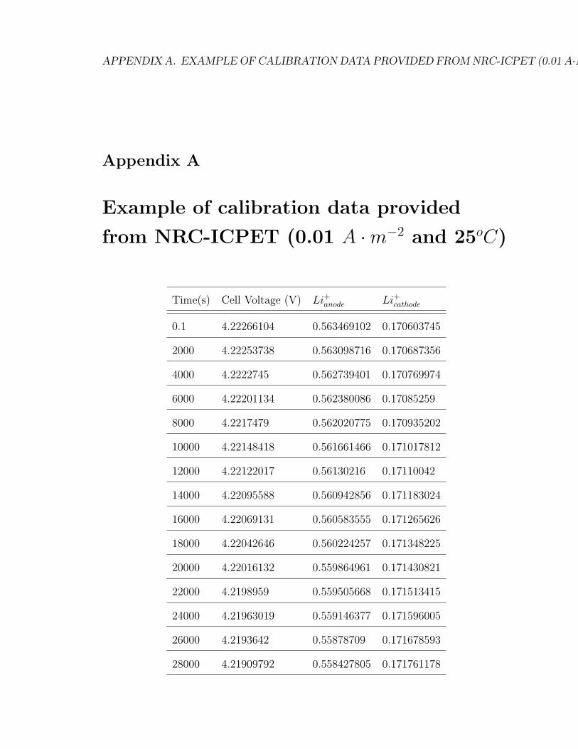
APPENDIX A. EXAMPLE OF CALIBRATION DATA PROVIDED FROM NRC-ICPET (0.01 A·M−2 AND 25OC)113
Appendix A
Example of calibration data provided
from NRC-ICPET (0.01 A ·m−2 and 25oC)
Time(s) Cell Voltage (V) Li+anode Li+cathode
0.1 4.22266104 0.563469102 0.170603745
2000 4.22253738 0.563098716 0.170687356
4000 4.2222745 0.562739401 0.170769974
6000 4.22201134 0.562380086 0.17085259
8000 4.2217479 0.562020775 0.170935202
10000 4.22148418 0.561661466 0.171017812
12000 4.22122017 0.56130216 0.17110042
14000 4.22095588 0.560942856 0.171183024
16000 4.22069131 0.560583555 0.171265626
18000 4.22042646 0.560224257 0.171348225
20000 4.22016132 0.559864961 0.171430821
22000 4.2198959 0.559505668 0.171513415
24000 4.21963019 0.559146377 0.171596005
26000 4.2193642 0.55878709 0.171678593
28000 4.21909792 0.558427805 0.171761178
Appendix B
Calibration parameters for the Li-ion
battery model
114

APPENDIX B. CALIBRATION PARAMETERS FOR THE LI-ION BATTERY MODEL115
IDSym
bol
Des
crip
tion
Units
1nPar
alnum
ber
ofce
lls
connec
ted
inpar
rallel
(−)
2nSer
ies
num
ber
ofce
lls
connec
ted
inse
ries
(−)
3ce
llC
apR
efre
fere
nce
capac
ity
for
aunit
cell
(Am
ph)
(Am
p.h)
4te
mpR
efbat
tery
refe
rence
oper
atin
gte
mper
ature
(oC
)
5m
axV
olt
DO
D=
0of
asi
ngl
ece
ll(V
)
6m
inVol
tD
OD
=10
0%
ofa
singl
ece
ll(V
)
7cu
rren
tMax
max
imum
char
ge/d
isch
arge
curr
ent
ofon
ece
ll(A
mps
)
8vo
ltM
axm
axim
um
char
ge/d
isch
arge
volt
age
ofon
ece
ll(V
)
9bat
Tem
pIn
itin
itia
lbat
tery
tem
per
ature
(%)
10bat
init
DO
Din
itia
lD
OD
(%)
11th
erm
alM
ass
ther
mal
mas
sof
asi
ngl
ece
llm
.Cp
(J.oC−
1)
12hea
tLos
sFac
thea
tlo
ssfa
ctor
h*A
(W.oC−
1)
13hea
ters
Res
resi
stan
ceof
the
hea
ters
(Ω)
14upper
Bou
ndD
OD
max
imum
DO
Dof
bat
tery
(%)
15lo
wer
Bou
ndD
OD
min
imum
DO
Dof
bat
tery
(%)
16te
mpM
axm
axim
um
bat
tery
tem
per
ature
(oC
)
17te
mpM
inm
inim
um
bat
tery
tem
per
ature
(oC
)
18E
5
19E
4**
****
****
****
*
20E
3O
CV
volt
age
asa
funct
ion
ofD
OD
ofa
singl
ece
ll
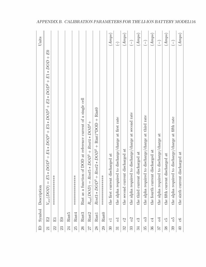
APPENDIX B. CALIBRATION PARAMETERS FOR THE LI-ION BATTERY MODEL116
IDSym
bol
Des
crip
tion
Unit
s
21E
2V
ocv
(DO
D)
=E
5∗
DO
D5+
E4∗
DO
D4+
E3∗
DO
D3+
E2∗
DO
D2+
E1∗
DO
D+
E0
22E
1**
****
****
****
*
23E
0
24R
int5
25R
int4
****
****
****
***
26R
int3
Rin
tas
afu
nct
ion
ofD
OD
atre
fere
nce
curr
ent
ofa
singl
ece
ll
27R
int2
Rin
t(D
OD
)=
Rin
t5∗
DO
D5+
Rin
t4∗
DO
D4+
28R
int1
Rin
t3∗
DO
D3+
Rin
t2∗
DO
D2
+R
int1
*DO
D+
Rin
t0
29R
int0
****
****
****
***
30c1
the
firs
tcu
rren
tdis
char
ged
at(A
mps
)
31α1
the
alpha
required
todis
char
ge/c
har
geat
firs
tra
te(-
)
32c2
the
seco
nd
curr
ent
dis
char
ged
at(A
mps
)
33α2
the
alpha
required
todis
char
ge/c
har
geat
seco
nd
rate
(−)
34c3
the
thir
dcu
rren
tdis
char
ged
at(A
mps
)
35α3
the
alpha
required
todis
char
ge/c
har
geat
thir
dra
te(−
)
36c4
the
fourt
hcu
rren
tdis
char
ged
at(A
mps
)
37α4
the
alpha
required
todis
char
ge/c
har
geat
(−)
38c5
the
fift
hcu
rren
tdis
char
ged
at(A
mps
)
39α5
the
alpha
required
todis
char
ge/c
har
geat
fift
hra
te(−
)
40c6
the
sixth
curr
ent
dis
char
ged
at(A
mps
)

APPENDIX B. CALIBRATION PARAMETERS FOR THE LI-ION BATTERY MODEL117
IDSym
bol
Des
crip
tion
Units
41α6
the
alpha
requir
edto
dis
char
ge/c
har
geat
sixth
rate
(−)
42c7
the
seve
nth
curr
ent
dis
char
ged
at(A
mps
)
43α7
the
alpha
requir
edto
dis
char
ge/c
har
geat
seve
nth
rate
(−)
44c8
the
eigh
thcu
rren
tdis
char
ged
at(A
mps
)
45α8
the
alpha
requir
edto
dis
char
ge/c
har
geat
eigh
thra
te(−
)
46T
1th
efirs
tte
mper
ature
dis
char
ged/c
har
ged
at(o
C)
47β1
the
bet
are
quir
edto
dis
char
ge/c
har
geat
the
firs
tte
mper
ature
(−)
48∆
V(T
)1th
evo
ltag
eoff
set
requir
edto
dis
char
ge/c
har
geat
the
firs
tte
mper
ature
(V)
49T
2th
ese
cond
tem
per
ature
dis
char
ged/c
har
ged
at(o
C)
50β2
the
bet
are
quir
edto
dis
char
ge/c
har
geat
the
seco
nd
tem
per
ature
(−)
51∆
V(T
)2th
evo
ltag
eoff
set
requir
edto
dis
char
ge/c
har
geat
the
seco
nd
tem
per
ature
(V)
52T
3th
eth
ird
tem
per
ature
dis
char
ged/c
har
ged
at(o
C)
53β3
the
bet
are
quir
edto
dis
char
ge/c
har
geat
the
thir
dte
mper
ature
(−)
54∆
V(T
)3th
evo
ltag
eoff
set
requir
edto
dis
char
ge/c
har
geat
the
third
tem
per
ature
(V)
55T
4th
efo
urt
hte
mper
ature
dis
char
ged/c
har
ged
at(o
C)
56β4
the
bet
are
quir
edto
dis
char
ge/c
har
geat
the
fourt
hte
mper
ature
(−)
57∆
V(T
)4th
evo
ltag
eoff
set
requir
edto
dis
char
ge/c
har
geat
the
fourt
hte
mper
ature
(V)
58T
5th
efift
hte
mper
ature
dis
char
ged/c
har
ged
atin
(oC
)
59β5
the
bet
are
quir
edto
dis
char
ge/c
har
geat
the
fift
hte
mper
ature
(−)
60∆
V(T
)5th
evo
ltag
eoff
set
requir
edto
dis
char
ge/c
har
geat
the
fift
hte
mper
ature
(V)

APPENDIX B. CALIBRATION PARAMETERS FOR THE LI-ION BATTERY MODEL118
IDSym
bol
Des
crip
tion
Unit
s
61T
6th
esi
xth
tem
per
ature
dis
char
ged/c
har
ged
at(o
C)
62β6
the
bet
are
quir
edto
dis
char
ge/c
har
geat
the
sixth
tem
per
ature
(−)
63∆
V(T
)6th
evo
ltag
eoff
set
requir
edto
dis
char
ge/c
har
geat
the
sixth
tem
per
ature
(V)
64T
7th
ese
venth
tem
per
ature
dis
char
ged/c
har
ged
at(o
C)
65β7
the
bet
are
quir
edto
dis
char
ge/c
har
geat
the
seve
nth
tem
per
ature
(−)
66∆
V(T
)7th
evo
ltag
eoff
set
requir
edto
dis
char
ge/c
har
geat
the
seve
nth
tem
per
ature
(V)
67T
8th
eei
ghth
tem
per
ature
dis
char
ged/c
har
ged
at(o
C)
68β8
the
bet
are
quir
edto
dis
char
ge/c
har
geat
the
eigh
thte
mper
ature
(−)
69∆
V(T
)8th
evo
ltag
eoff
set
requir
edto
dis
char
ge/c
har
geat
the
eigh
thte
mper
ature
(V)
70k
ose
lfdis
char
geco
nst
ant
(A)
71E
as
acti
vati
onen
ergy
for
self-d
isch
arge
(kJ).
(km
ol)−
1
72iZ
oneI
ndex
the
index
ofth
ezo
ne
wher
eth
ebat
tery
islo
cate
d(−
)
73pPar
asit
icth
epow
erre
quir
edto
run
the
li-ion
BM
Sci
rcuit
ry(W
)
74R
intH
i5**
****
****
****
*
75R
intH
i4SE
CO
ND
OP
TIO
NA
LR
int
asa
funct
ion
ofD
OD
atre
fere
nce
curr
ent
ofa
singl
ece
ll
76R
intH
i3R
int(
DO
D)
=R
int5∗
DO
D5+
Rin
t4∗
DO
D4+
Rin
t3∗
DO
D3
77R
intH
i2+
Rin
t2∗
DO
D2+
Rin
t1∗
DO
D+
Rin
t0
78R
intH
i1if
any
ofth
ese
equal
999.
they
willbe
over
riden
and
only
the
firs
tse
t(2
4-29
)w
illbe
use
d
79R
intH
i0ot
her
wis
eth
isw
illbe
use
dfo
rI
gtIfl
agan
d(2
4-29
)w
illbe
use
dfo
rI
ltIfl
ag
80Ifl
agC
urr
ent
valu
efo
rif
the
curr
ent
ishig
her
the
seco
nd
set
ofR
int
willbe
use
d(A
)
81C
ycl
e cruc
The
cruci
alcy
cle
toin
dic
ate
the
end
ofth
ece
ll’s
life


