Towards Region Discovery in Spatial Datasets

Wei Ding1??, Rachsuda Jiamthapthaksin1, Rachana Parmar1, Dan Jiang1,Tomasz F. Stepinski2, and Christoph F. Eick1

1 University of Houston, Houston TX 77204-3010, USA{wding,rachsuda,rparmar,djiang,ceick}@uh.edu

2 Lunar and Planetary Institute, Houston, TX 77058, USAtstepinski@lpi.usra.edu

Abstract. This paper presents a novel region discovery framework gearedtowards finding scientifically interesting places in spatial datasets. Weview region discovery as a clustering problem in which an externallygiven fitness function has to be maximized. The framework adapts fourrepresentative clustering algorithms, exemplifying prototype-based, grid-based, density-based, and agglomerative clustering algorithms, and thenwe systematically evaluated the four algorithms in a real-world casestudy. The task is to find feature-based hotspots where extreme den-sities of deep ice and shallow ice co-locate on Mars. The results revealthat the density-based algorithm outperforms other algorithms inasmuchas it discovers more regions with higher interestingness, the grid-basedalgorithm can provide acceptable solutions quickly, while the agglom-erative clustering algorithm performs best to identify larger regions ofarbitrary shape. Moreover, the results indicate that there are only a fewregions on Mars where shallow and deep ground ice co-locate, suggestingthat they have been deposited at different geological times.

Key words: Region Discovery, Clustering, Hotspot Discovery, SpatialData Mining

1 Introduction

The goal of spatial data mining [1–3] is to automate the extraction of interest-ing and useful patterns that are not explicitly represented in spatial datasets.Of particular interests to scientists are the techniques capable of finding sci-entifically meaningful regions as they have many immediate applications ingeoscience, medical science, and social science; e.g., detection of earthquakehotspots, disease zones, and criminal locations. An ultimate goal for regiondiscovery is to provide search-engine-style capabilities to scientists in a highlyautomated fashion. Developing such a system faces the following challenges.First, the system must be able to find regions of arbitrary shape at differ-ent levels of resolution. Second, the system needs to provide suitable, plug-inmeasures of interestingness to instruct discovery algorithms what they shouldseek for. Third, the identified regions should be properly ranked by relevance.

?? Also, Computer Science Department, University of Houston-Clear Lake.

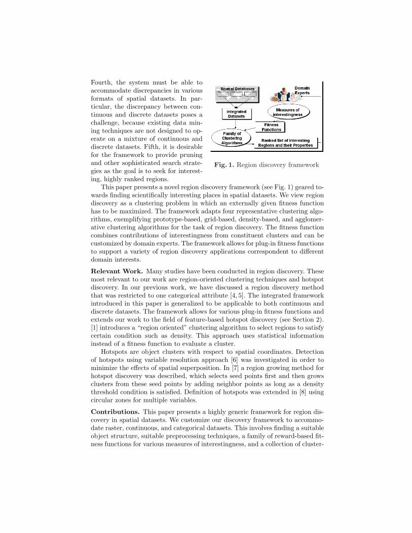
Fig. 1. Region discovery framework

Fourth, the system must be able toaccommodate discrepancies in variousformats of spatial datasets. In par-ticular, the discrepancy between con-tinuous and discrete datasets poses achallenge, because existing data min-ing techniques are not designed to op-erate on a mixture of continuous anddiscrete datasets. Fifth, it is desirablefor the framework to provide pruningand other sophisticated search strate-gies as the goal is to seek for interest-ing, highly ranked regions.

This paper presents a novel region discovery framework (see Fig. 1) geared to-wards finding scientifically interesting places in spatial datasets. We view regiondiscovery as a clustering problem in which an externally given fitness functionhas to be maximized. The framework adapts four representative clustering algo-rithms, exemplifying prototype-based, grid-based, density-based, and agglomer-ative clustering algorithms for the task of region discovery. The fitness functioncombines contributions of interestingness from constituent clusters and can becustomized by domain experts. The framework allows for plug-in fitness functionsto support a variety of region discovery applications correspondent to differentdomain interests.

Relevant Work. Many studies have been conducted in region discovery. Thesemost relevant to our work are region-oriented clustering techniques and hotspotdiscovery. In our previous work, we have discussed a region discovery methodthat was restricted to one categorical attribute [4, 5]. The integrated frameworkintroduced in this paper is generalized to be applicable to both continuous anddiscrete datasets. The framework allows for various plug-in fitness functions andextends our work to the field of feature-based hotspot discovery (see Section 2).[1] introduces a “region oriented” clustering algorithm to select regions to satisfycertain condition such as density. This approach uses statistical informationinstead of a fitness function to evaluate a cluster.

Hotspots are object clusters with respect to spatial coordinates. Detectionof hotspots using variable resolution approach [6] was investigated in order tominimize the effects of spatial superposition. In [7] a region growing method forhotspot discovery was described, which selects seed points first and then growsclusters from these seed points by adding neighbor points as long as a densitythreshold condition is satisfied. Definition of hotspots was extended in [8] usingcircular zones for multiple variables.

Contributions. This paper presents a highly generic framework for region dis-covery in spatial datasets. We customize our discovery framework to accommo-date raster, continuous, and categorical datasets. This involves finding a suitableobject structure, suitable preprocessing techniques, a family of reward-based fit-ness functions for various measures of interestingness, and a collection of cluster-

ing algorithms. We systematically evaluate a wide range of representative clus-tering algorithms to determine when and which type of clustering techniquesare more suitable for region discovery. We apply our framework to a real-worldcase study concerning ground ice on Mars and successfully find scientificallyinteresting places.

2 Methodology

Region Discovery Framework. Our region discovery method employs a reward-based evaluation scheme that evaluates the quality of the discovered regions.Given a set of regions R = {r1, . . . , rk} identified from a spatial dataset O ={o1, . . . , on}, the fitness of R is defined as the sum of the rewards obtained fromeach region rj (j = 1 . . . k):

q(R) =k∑

j=1

(i(rj)× size(rj)β) (1)

where i(rj) is the interestingness measure of region rj – a quantity based ondomain interest to reflect the degree to which the region is “newsworthy”. Theframework seeks for a set of regions R such that the sum of rewards over all of itsconstituent regions is maximized. size(rj)β (β > 1) in q(R) increases the valueof the fitness nonlinearly with respect to the number of objects in O belongingto the region rj . A region reward is proportional to its interestingness, but giventwo regions with the same value of interestingness, a larger region receives ahigher reward to reflect a preference given to larger regions.

We employ clustering algorithms for region discovery. A region is a contiguoussubspace that contains a set of spatial objects: for each pair of objects belongingto the same region, there always exists a path within this region that connectsthem. We search for regions r1, . . . , rk such that:

1. ri ∩ rj = ∅, i 6= j. The regions are disjoint.2. R = {r1, . . . , rk} maximizes q(R).3. r1 ∪ . . . ∪ rk ⊆ O. The generated regions are not required to be exhaustive

with respect to the global dataset O.4. r1, . . . , rk are ranked based on their reward values. Regions that receive no

reward are discarded as outliers.

Preprocessing. Preprocessing techniques are introduced to facilitate the appli-cation of the framework to heterogeneous datasets. Given a collection of raster,categorical, and continuous datasets with a common spatial extent, the rasterdatasets are represented as (<pixel>, <continuous variables>), the categoricaldataset as (<point>, <category variables>)3, and the continuous datasets as(<point>, <continuous variables>). Fig. 2 depicts our preprocessing procedure:

3 To deal with multiple categorical datasets a single dataset can be constructed bytaking the union of multiple categorical datasets.

Fig. 2. Preprocessing for heterogeneous spatial datasets

Step 1. Dataset Integration Categorical datasets are converted into a con-tinuous density dataset (<point>, <density variables>), where a densityvariable describes the density of a class for a given point. Classical densityestimation techniques [9], such as Gaussian kernel functions, can be used forsuch transformation. Raster datasets are mapped into point datasets usinginterpolation functions that compute point values based on the raster values.

Step 2. Dataset Unification A single unified spatial dataset is created bytaking a natural join on the spatial attributes of each dataset. Notice thatthe datasets have to be made “join compatible” in Step 1. This can beaccomplished by using the same set of points in each individual dataset.

Step 3. Dataset Normalization Finally, continuous variables are normalizedinto z-scores to produce a generic dataset O=(<point>, <z-scores>), wherez-score is the number of standard deviations that a given value is above orbelow the mean.

Measure of Interestingness. The fitness function q(R) (Eqn. 1) allows afunction of interestingness to be defined based on different domain interests.In our previous work, we have defined fitness functions to search risk zones ofearthquakes [4] and volcanoes [5] with respect to a single categorical attribute.In this paper, we define feature-based hotspots as localized regions where contin-uous non-spatial features of objects attain together the values from the wingsof their respective distributions. Hence our feature-based hotspots are placeswhere multiple, potentially globally uncorrelated attributes happen to attainextreme values. We then introduce a new interestingness function i on the topof the generic dataset O: given set of continuous features A = {A1, ..., Aq} theinterestingness of an object o ∈ O is measured as follows:

i(A, o) =q∏

j=1

zAj (o) (2)

where zAj(o) is the z-score of the continuous feature Aj . Objects with |i(A, o)| À

0 are clustered in feature-based hotspots where the features in A happen to attainextreme values—measured as products of z-scores.

We then extend the definition of interestingness to regions: the interestingnessof a region r is the absolute value of the average interestingness of the objectsbelonging to it:

i(A, r) =

{( |Σo∈r i(A,o)|

size(r) − zth) if |Σo∈r i(A,o)|size(r) > zth

0 otherwise.(3)

In Eqn. 3 the interestingness threshold zth is introduced to weed out regionswith i(r) close to 0, which prevents clustering solutions from containing onlylarge clusters of low interestingness.

Clustering Algorithms. Our regional discovery framework relies on reward-based fitness functions. Consequently, clustering algorithms embedded in theframework, have to allow for plug-in fitness functions. However, the use of fitnessfunction is quite uncommon in clustering, although a few exceptions exist, e.g.,CHAMELEON [10]. Furthermore, region discovery is different from traditionalclustering as it gears to find interesting places with respect to a given measureof interestingness. Consequently, existing clustering techniques need to be mod-ified extensively for the task of region discovery. The proposed region discoveryframework adapts a family of prototype-based, agglomerative, density-based,and grid-based clustering approaches. We give a brief survey of these algorithmsin this section.

Prototype-based Clustering Algorithms. Prototype-based clustering al-gorithms first seek for a set of representatives; clusters are then created by as-signing objects in the dataset to the closest representatives. We introduce amodification of the PAM algorithm [11] which we call SPAM (Supervised PAM).SPAM starts its search with a random set of k representatives, and then greed-ily replaces representatives with non-representatives as long as q(R) improves.SPAM requires the number of clusters, k, as an input parameter. Fig. 3a illus-trates the application of SPAM to a supervised clustering task in which purity ofclusters with respect to the instances of two classes has to be maximized. SPAMcorrectly separates cluster A from cluster B because the fitness value would bedecreased if the two clusters were merged, while the traditional PAM algorithmwill merge the two clusters because they are in close proximity.

Agglomerative Algorithms. Due to the fact that prototype-based algo-rithms construct clusters using nearest neighbor queries, the shape of clustersidentified are limited to convex polygons (Voronoi cells). Interesting regions, andin particular, hotspots, may not be restricted to convex shapes. Agglomerativeclustering algorithms are capable of yielding solutions with clusters of arbitraryshape by constructing unions of small convex polygons. We adapt the MOSAICalgorithm [5] that takes a set of small convex clusters as its input and greed-ily merges neighboring clusters as long as q(R) improves. In our experimentsthe inputs are generated by the SPAM algorithm. Gabriel graphs [12] are used

Fig. 3. Clustering algorithms

to determine which clusters are neighbors. The number of clusters, k, is thenimplicitly determined by the clustering algorithm itself. Fig. 3b illustrates thatMOSAIC identifies 9 clusters (4 of them are in non-convex shape) from the 95small convex clusters generated by SPAM.

Density-Based Algorithms. Density-based algorithms construct clustersfrom an overall density function. We adapt the SCDE (Supervised ClusteringUsing Density Estimation) algorithm [13] to search feature-based hotspots. Eachobject o in O is assigned a value of i(A, o) (see Eqn. 2). The influence function ofobject o, fGauss(p, o), is defined as the product of i(A, o) and a Gaussian kernel:

fGauss(p, o) = i(A, o)× e−d(p,o)2

2σ2 . (4)

The parameter σ determines how quickly the influence of o on p decreases asthe distance between o and p increases. The density function, Ψ(p) at point p isthen computed as:

Ψ(p) =∑

o∈O

fGauss(p, o). (5)

Unlike traditional density estimation techniques, which only consider the spa-tial distance between data points, our density estimation approach additionallyconsiders the influence of the interestingness i(A, o). SCDE uses a hill climbingapproach to compute local maxima and local minima of the density function Ψ .These locales act as cluster attractors; clusters are formed by associating objectsin O with the attractors. The number of clusters, k, is implicitly determined bythe parameter σ. Fig. 3c illustrates an example in which SCDE identifies 9 re-gions that are associated with maxima (in red) and minima (in blue) of thedepicted density function on the right.

Grid-based Algorithms. SCMRG (Supervised Clustering using Multi-Resolution Grids) [4] is a hierarchical, grid-based method that utilizes a divisive,top-down search. The spatial space of the dataset is partitioned into grid cells.

Each grid cell at a higher level is partitioned further into smaller cells at thelower level, and this process continues as long as the sum of the rewards of thelower level cells q(R) is not decreased. The regions returned by SCMRG arecombination of grid cells obtained at different level of resolution. The number ofclusters, k, is calculated by the algorithm itself. Fig. 3d illustrates that SCMRGdrills down 3 levels and identifies 2 clusters (the rest of cells are discarded asoutliers due to low interestingness).

3 A Real-World Case Study: Ground Ice on Mars

Dataset Description and Preprocessing. We systematically evaluate ourregion discovery framework on spatial distribution of ground ice on Mars. Marsis at the center of the solar system exploration efforts. Finding scientificallyinteresting places where shallow and deep ice abundances coincide provides im-portant insight into the history of water on Mars. Shallow ice located in theshallow subsurface of Mars, within an upper 1 meter, is obtained remotely fromorbit by the gamma-ray spectrometer [14] (see Fig. 4a, shallow ice in 5o × 5o

resolution). A spatial distribution of deep ice, up to the depth of a few kilo-meters, can be inferred from spatial distribution of rampart craters [15] (seeFig. 4b, distribution of 7559 rampart craters restricted to the spatial extent de-fined by the shallow ice raster). Rampart craters, which constitute about 20%of all the 35927 craters on Mars, are surrounded by ejecta that have patternslike splashes and are thought to form in locations once rich in subsurface ice.Locally-defined relative abundance of rampart craters can be considered a proxyfor the abundance of deep ice.

Using the preprocessing procedure outlined in Section 2 we construct ageneric dataset (<longitude, latitude>, zdi, zsi) where <longitude, latitude>is the coordinate of each rampart crater, zdi denotes the z-score of deep ice andzsi denotes the z-score of shallow ice. The values of these two features at locationp are computed using a 5o × 5o moving window wrapped around p. The shallowice feature is an average of shallow-ice abundances as measured at locations ofobjects within the window, and the deep-ice feature is a ratio of rampart to allthe craters located within the window.

Region Discovery Results. SPAM, MOSAIC, SCDE, and SCMRG clusteringalgorithms are used to find feature-based hotspots where extreme values of deepice and shallow ice co-locate on Mars. The algorithms have been developed inour open source project Cougar2 Java Library for Machine Learning and DataMining Algorithms [16]. In the experiments, the clustering algorithms maximizethe following fitness function q(R) — see also Eqn 1:

q(R) =∑

r∈R

(i({zdi, zsi}, r)× size(r)β) (6)

For the purpose of simplification, we will use z for i({zdi, zsi}, r) in the rest of thepaper. In the experiments, the interestingness threshold is set to be zth = 0.15and two different β values are used: β = 1.01 is used for finding stronger hotspots

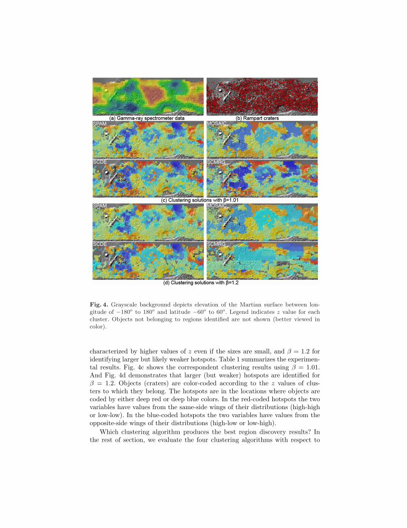
Fig. 4. Grayscale background depicts elevation of the Martian surface between lon-gitude of −180o to 180o and latitude −60o to 60o. Legend indicates z value for eachcluster. Objects not belonging to regions identified are not shown (better viewed incolor).

characterized by higher values of z even if the sizes are small, and β = 1.2 foridentifying larger but likely weaker hotspots. Table 1 summarizes the experimen-tal results. Fig. 4c shows the correspondent clustering results using β = 1.01.And Fig. 4d demonstrates that larger (but weaker) hotspots are identified forβ = 1.2. Objects (craters) are color-coded according to the z values of clus-ters to which they belong. The hotspots are in the locations where objects arecoded by either deep red or deep blue colors. In the red-coded hotspots the twovariables have values from the same-side wings of their distributions (high-highor low-low). In the blue-coded hotspots the two variables have values from theopposite-side wings of their distributions (high-low or low-high).

Which clustering algorithm produces the best region discovery results? Inthe rest of section, we evaluate the four clustering algorithms with respect to

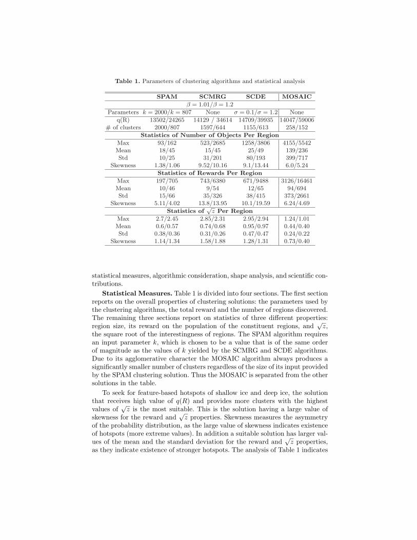
Table 1. Parameters of clustering algorithms and statistical analysis

SPAM SCMRG SCDE MOSAIC

β = 1.01/β = 1.2

Parameters k = 2000/k = 807 None σ = 0.1/σ = 1.2 None

q(R) 13502/24265 14129 / 34614 14709/39935 14047/59006# of clusters 2000/807 1597/644 1155/613 258/152

Statistics of Number of Objects Per Region

Max 93/162 523/2685 1258/3806 4155/5542Mean 18/45 15/45 25/49 139/236Std 10/25 31/201 80/193 399/717

Skewness 1.38/1.06 9.52/10.16 9.1/13.44 6.0/5.24

Statistics of Rewards Per Region

Max 197/705 743/6380 671/9488 3126/16461Mean 10/46 9/54 12/65 94/694Std 15/66 35/326 38/415 373/2661

Skewness 5.11/4.02 13.8/13.95 10.1/19.59 6.24/4.69

Statistics of√

z Per Region

Max 2.7/2.45 2.85/2.31 2.95/2.94 1.24/1.01Mean 0.6/0.57 0.74/0.68 0.95/0.97 0.44/0.40Std 0.38/0.36 0.31/0.26 0.47/0.47 0.24/0.22

Skewness 1.14/1.34 1.58/1.88 1.28/1.31 0.73/0.40

statistical measures, algorithmic consideration, shape analysis, and scientific con-tributions.

Statistical Measures. Table 1 is divided into four sections. The first sectionreports on the overall properties of clustering solutions: the parameters used bythe clustering algorithms, the total reward and the number of regions discovered.The remaining three sections report on statistics of three different properties:region size, its reward on the population of the constituent regions, and

√z,

the square root of the interestingness of regions. The SPAM algorithm requiresan input parameter k, which is chosen to be a value that is of the same orderof magnitude as the values of k yielded by the SCMRG and SCDE algorithms.Due to its agglomerative character the MOSAIC algorithm always produces asignificantly smaller number of clusters regardless of the size of its input providedby the SPAM clustering solution. Thus the MOSAIC is separated from the othersolutions in the table.

To seek for feature-based hotspots of shallow ice and deep ice, the solutionthat receives high value of q(R) and provides more clusters with the highestvalues of

√z is the most suitable. This is the solution having a large value of

skewness for the reward and√

z properties. Skewness measures the asymmetryof the probability distribution, as the large value of skewness indicates existenceof hotspots (more extreme values). In addition a suitable solution has larger val-ues of the mean and the standard deviation for the reward and

√z properties,

as they indicate existence of stronger hotspots. The analysis of Table 1 indicates

that SCDE and SCMRG algorithms are more suitable to discovery hotspots withhigher values in z. Furthermore, we are interested in evaluating the search capa-bility, how the top n regions are selected by the four algorithms. Fig. 5a illustratesthe average region size with respect to the top 99th, 97th, 94th, 90th, 80th, 60th

percentile for the value of interetingness z. Fig. 5b depicts the average value ofinterestingness per cluster with respect to the top 10 largest regions. We ob-serve that SCDE can pinpoint stronger hotspots in smaller size (e.g., size = 4and z = 5.95), while MOSAIC is the better algorithm for larger hotspots withrelatively higher value of interestingness (e.g., size = 2096 and z = 1.38).

Algorithmic Considerations. As determined by the nature of the algo-rithm, SCDE and SCMRG algorithms support the notion of outliers – bothalgorithms evaluate and prune low-interest regions (outliers) dynamically dur-ing the search procedure. Outliers create an overhead for MOSAIC and SPAMbecause both algorithms are forced to create clusters to separate non-rewardregions (outliers) from reward regions. Assigning outliers to a reward region inproximity is not an alternative because this would lead to a significant drop inthe interestingness value and therefore to a significant drop in total rewards.

The computer used in our experiments is Intel(R) Xeon, CPU 3.2GHz, 1GBof RAM. In the experiments of β = 1.01 the SCDE algorithm takes ∼ 500s tocomplete, whereas the SCMRG takes ∼ 3.5s, the SPAM takes ∼ 50000s, and theMOSAIC took ∼ 155000s. Thus, the SCMRG algorithm is significantly fasterthan the other clustering algorithms and, on this basis, it could be a suitablecandidate to searching for hotspots in a very large dataset with limited time.

Shape Analysis. As depicted in Fig. 4, in con-trast to SPAM whose shapes are limited to convexpolygons, and SCMRG whose shapes are limited tounions of grid-cells, MOSAIC and SCDE can findarbitrary-shaped clusters. The SCMRG algorithmonly produces good solutions for small values of β,as larger values of β lead to the formation of large,boxy segments that are not effective in isolating thehotspots. In addition, the figure on the right depictsthe area of Acidalia Plantia on Mars (centered at ∼ −15o longitude, −40o lati-tude). MOSAIC and SCDE have done a good job in finding non-convex shapeclusters. Moveover, notice that both algorithms can discover interesting regionsinside other regions – red-coded regions (high-high or low-low) are successfullyidentified inside the blue-coded regions (low-high or high-low). It thus makes thehotspots even “hotter” when excluding inside regions from an outside region.

Scientific Contributions. Although the global correlation between theshallow ice and deep ice variables is only −0.14434 — suggesting the absence of aglobal linear relationship — our region discovery framework has found a numberof local regions where extreme values of both variables co-locate. Our results in-dicate that there are several regions on Mars that show a strong anti-collocationbetween shallow and deep ice (in blue), but there are only few regions on Marswhere shallow and deep ground ice co-locate (in red). This suggests that shallow

Fig. 5. Search capability evaluation.

ice and deep ice have been deposited at different geological times on Mars. Theseplaces need to be further studied by the domain experts to find what particularset of geological circumstances led to their existence.

4 Conclusion

This paper presents a novel region discovery framework for identifying the feature-based hotspots in spatial datasets. We have evaluated the framework with areal-world case study of spatial distribution of ground ice on Mar. Empiricalstatistical evaluation was developed to compare the different clustering solutionsfor their effectiveness in locating hotspots. The results reveal that the density-based SCDE algorithm outperforms other algorithms inasmuch as it discoversmore regions with higher interestingness, the grid-based SCMRG algorithm canprovide acceptable solutions within limited time, while the agglomerative MO-SAIC clustering algorithm performs best on larger hotspots of arbitrary shape.Furthermore, our region discovery algorithms have identified several interestingplaces on Mars that will be further studied in the application domain.

5 Acknowledgments

The work is supported in part by the National Science Foundation under GrantIIS-0430208. A portion of this research was conducted at the Lunar and Plane-tary Institute, which is operated by the USRA under contract CAN-NCC5-679with NASA.

References

1. Wang, W., Yang, J., Muntz, R.R.: STING: A statistical information grid approachto spatial data mining. In: 23rd Intl. Conf. on Very Large Data Bases. (1997)

2. Koperski, K., Han, J.: Discovery of spatial association rules in geographic infor-mation databases. In Egenhofer, M.J., Herring, J.R., eds.: Procs. of the 4th Intl.Symp. Advances in Spatial Databases. Volume 951. (6–9 1995) 47–66

3. Shekhar, S., Huang, Y.: Discovering spatial co-location patterns: A summary ofresults. Lecture Notes in Computer Science 2121 (2001)

4. Eick, C.F., Vaezian, B., Jiang, D., Wang, J.: Discovering of interesting regionsin spatial data sets using supervised clustering. In: The 10th European Conf. onPrinciples and Practice of Knowledge Discovery in Databases (PKDD’06). (2006)

5. Choo, J., Jiamthapthaksin, R., sheng Chen, C., Celepcikay, O.U., Giusti, C., Eick,C.F.: MOSAIC: A proximity graph approach for agglomerative clustering. In: The9th Intl. Conf. on Data Warehousing and Knowledge Discovery. (2007)

6. Brimicombe, A.J.: Cluster detection in point event data having tendency towardsspatially repetitive events. In: the 8th Intl. Conf. on GeoComputation. (2005)

7. Tay, S.C., Hsu, W., Lim., K.H.: Spatial data mining: Clustering of hot spots andpattern recognition. In: the Intl. Geoscience & Remote Sensing Symposium. (2003)

8. Kulldorff, M.: Prospective time periodic geographical disease surveillance using ascan statistic. Journal Of The Royal Statistical Society Series A 164 (2001) 61–72

9. Silverman, B.: Density Estimation for Statistics and Data Analysis. Chapman &Hall (1986)

10. Karypis, G., Han, E.H.S., Kumar, V.: Chameleon: Hierarchical clustering usingdynamic modeling. IEEE Computer 32(8) (1999) 68–75

11. Kaufman, L., Rousseeuw, P.J.: Finding Groups in Data: An Introduction to ClusterAnalysis. John Wiley & Sons (1990)

12. Gabriel, K.R., Sokal, R.R.: A new statistical approach to geographic variationanalysis. Systematic Zoology 18 (1969) 259–278

13. Jiang, D., Eick, C.F., Chen, C.: On supervised density estimation techniques andtheir application to clustering. In: Procs. of the 15th ACM Intl. Symposium onAdvances in Geographic Information Systems. (2007)

14. Feldman, W.C.: Global distribution of near-surface hydrogen on mars. J. Geophys.Res. 109 E09006 (2004)

15. Barlow, N.G.: Crater size-distribution and a revised martian relative chronology.Icarus 75(20) (1988) 285–305

16. Data Mining and Machine Learning Group, University of Houston:https://cougarsquared.dev.java.net/, CougarSquared Data Mining and Ma-chine Learning Framework. (2007)