Towards Reducing Taxicab Cruising Time UsingSpatio-Temporal Profitability Maps

Jason W. Powell1, Yan Huang1, Favyen Bastani1, and Minhe Ji2

1 University of North Texas{jason.powell, huangyan??}@unt.edu, FavyenBastani@my.unt.edu

2 East China Normal Universitymhji@geo.ecnu.edu.cn

Abstract. Taxicab service plays a vital role in public transportationby offering passengers quick personalized destination service in a semi-private and secure manner. Taxicabs cruise the road network looking fora fare at designated taxi stands or alongside the streets. However, thisservice is often inefficient due to a low ratio of live miles (miles with afare) to cruising miles (miles without a fare). The unpredictable natureof passengers and destinations make efficient systematic routing a chal-lenge. With higher fuel costs and decreasing budgets, pressure mountson taxicab drivers who directly derive their income from fares and spendanywhere from 35-60 percent of their time cruising the road network forthese fares. Therefore, the goal of this paper is to reduce the number ofcruising miles while increasing the number of live miles, thus increasingprofitability, without systematic routing. This paper presents a simpleyet practical method for reducing cruising miles by suggesting profitablelocations to taxicab drivers. The concept uses the same principle that ataxicab driver uses: follow your experience. In our approach, historicaldata serves as experience and a derived Spatio-Temporal Profitability(STP) map guides cruising taxicabs. We claim that the STP map isuseful in guiding for better profitability and validate this by showing apositive correlation between the cruising profitability score based on theSTP map and the actual profitability of the taxicab drivers. Experimentsusing a large Shanghai taxi GPS data set demonstrate the effectivenessof the proposed method.

Key words: Profitability, Spatial, Temporal, Spatio-temporal, Taxi, Taxicabs

1 Introduction

Taxicab service plays a vital role in public transportation by offering passengersquick personalized destination service in a semi-private and secure manner. A2006 study reported that 241 million people rode New York City Yellow Medal-lion taxicabs and taxis performed approximately 470,000 trips per day, gener-ating $1.82 billion in revenue. This accounted for 11% of total passengers, an?? This work was partially supported by the National Science Foundation under Grant

No. IIS-1017926.

2

estimated 30% of total public transportation fares, and yielded average driverincome per shift of $158 dollars [1]. Taxicab drivers earn this by cruising theroad network looking for a passenger at designated taxi stands or alongside thestreets. However, this service is often inefficient from expensive vehicles with lowcapacity utilization, high fuel costs, heavily congested traffic, and a low ratio oflive miles (miles with a fare) to cruising miles (miles without a fare).

With higher fuel costs and decreasing budgets, pressure mounts on taxicabdrivers who directly derive their income from fares yet spend anywhere from35-60 percent of their time cruising the road network for fares [1]. The unpre-dictable nature of passengers and destinations make efficient systematic routinga challenge. Therefore, the goal is simultaneously reducing cruising miles whileincreasing live miles, thus increasing profitability, without systematic routing.

This paper presents a simple yet practical method for suggesting profitablelocations that enable taxicab drivers to reduce cruising miles. The concept usesthe same principle that a taxicab driver uses: follow your experience. We proposea framework to guide taxi drivers in locating fares. Specifically, this paper makesthree contributions. First, the proposed framework uses historical GPS datato model the potential profitability of locations given the current location andtime of a taxi driver. This model considers the main factors contributing to theprofitability: time and the profit loss associated with reaching a location. Second,this framework makes personalized suggestions to a taxi driver based on locationand time. This avoids the problem of communicating the same information to alldrivers, which may result in non-equilibrium in supply and demand. Third, wedemonstrate the effectiveness of the proposed framework using a large datasetof Shanghai taxicab GPS traces and use correlation to compare the suggestedlocations with actual driver behavior.

2 Related Work

Taxicab service falls into two general categories and research follows this, oc-casionally attempting to bridge them. The first category is dispatching wherecompanies dispatch taxicabs to customer requested specific locations. A requestmay be short-term (e.g., a customer requests a taxi for pickup within the next20 minutes) or long-term (e.g., arrangements come hours or days in advance).Logic dictates that the farther in advance the request, the easier it is to planefficient taxi service because routing algorithms already exist (mostly based onDijkstra’s work); the shorter the request time, the more challenging the routingproblem. The second category is cruising. The taxicab driver cruises the roadnetwork looking for a fare at designated taxi stands or alongside the streets, us-ing experience as a guide. This leads to an inefficient system where taxi driversspend significant time without a fare and often serve hot spots, leading to a sup-ply and demand imbalance. Since cruising is a profit loss, this paper will referto non-live miles as a cruising trip and live miles as a live trip. The followinghighlights some recent research in this area.

3

Yamamoto et al. propose a fuzzy clustering based dynamic routing algorithmin [2]. Using a taxicab driver’s daily logs, the algorithm creates an optimal routesolution based on passenger frequency on links (i.e., paths). The routes, notintended to be used directly by the taxi driver, are shared among taxis throughmutual exchanges (i.e., path sharing) that assigns the most efficient path toa taxi as they cruise. This potentially reduces the competition for a potentialfare, excessive supply to popular areas, and traffic congestion while increasingprofitability. Similarly, Li et al. present an algorithm using taxi GPS tracesto create a usage based road segment hierarchy from the frequency of taxistraversing a road segment [3]. This hierarchy inherently captures the taxi driverexperience and is usable in route planning. In these two examples, the focus ison routing but trip profitability—a key factor in the driver’s decision—is notexplicitly addressed.

Another example of taxicab routing is T-Drive, developed by Yuan et al.to determine the fastest route to a destination at a given departure time [16].T-Drive uses historical GPS trajectories to create a time-dependent landmarkgraph in which the nodes are road segments frequently traversed by taxis and avariance-entropy-based clustering approach determines the travel time distribu-tion between two landmarks for a given period. A novel routing algorithm thenuses this graph to find the fastest practical route in two stages. The first stage,rough routing, searches the graph for the fastest route for a sequence of land-marks; the second stage, refined routing, creates the real network route using therough route. Similar to the previous example, this system does inherently cap-ture taxi driver experience and suggests faster routes than alternative methods;however, this method does not suggest profitable locations for taxicabs.

A thesis by Han Wang proposes a methodology for combining short-term andlong-term dispatching [4]. If a customer’s starting and ending locations followthe path of a taxi as it heads to a different dispatch call, the taxi can pick upthe fare. This allows a reduction in cruising and an increase in profitability. Thecatch is that it may not be common for passenger routes to align exactly. There-fore, Wang proposes the Shift Match Algorithms that suggest drivers and/orcustomers to adjust locations, creating a reasonable short delay in service butan improvement overall. In this study, the cruise trips are different from thosein the aforementioned cruising category because they result from dispatching,not from intent to cruise. This method is practical for dispatching but not forgeneral cruising.

Another approach, given by Cheng et al., focuses on customer queuing at taxistands and taxis switching between serving stands and cruising [5]. Phithakkit-nukoon et al. developed an inference engine with error based learning to predictvacant taxis [6] while Hong-Cheng et al. studied travel time variability on driverroute choices in Shanghai taxi service [7]. Additional research covers a variety ofissues from demand versus supply to pricing issues [8–12]; however, these studiesdo not consider location profitability, which is inherent to the driver’s decision.

The work most similar to ours is by Ge et al., who provide a novel techniquein extracting energy-efficient transportation patterns from taxi trajectory traces

4

and a mobile recommender system for taxis [17]. The technique extracts a groupof successful taxi drivers and clusters their pick-up points into centroids withan assigned probability of successful pick-up. The resulting centroids becomethe basis for pick-up probability routes that the system distributes among taxisto improve overall business success. The major contribution is how the systemevaluates candidate routes using a monotonic Potential Travel Distance (PTD)function that their novel route-recommendation algorithm exploits to prune thesearch space. They also provide the SkyRoute algorithm that reduces the com-putational costs associated with skyline routes, which dominate the candidateroute set. This recommender system potentially improves success by using prob-abilities; however, probabilities can be misleading in relation to the profitabilitysince high probabilities do not necessarily translate into highly profitable livetrips. In addition, the algorithm clusters locations using fix periods regardlessof when the taxicab actually arrives at a location. Furthermore, our frameworksuggests a customized map of locations based on the taxicab’s current location toeliminate route creation cost and taxi-route assignment distribution issues; how-ever, their algorithms could enhance our framework by suggesting customizedpaths for the taxi driver using a time series of STP maps.

3 Methodology

The taxicab driver is not concerned with finding profitable locations during alive trip. Once the live trip is complete, assuming there is not a new passengeravailable at the location, the driver must decide where to go. They may stay inthat general vicinity for a time in hopes of a passenger or, more likely, head toanother location based on experience. At this moment, the driver considers twovariables: profitable locations and reasonable driving distances. However, a drivermight be unaware of both variables. For example, a driver may be unreasonablyfar from a highly profitable airport but unsure of closer profitable locations lessoften visited. Given a map identifying these locations, the driver can make aninformed decision quickly and reduce cruising time.

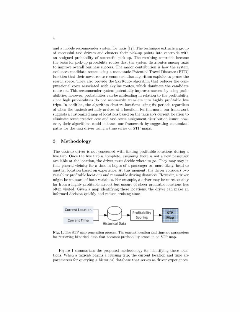
Fig. 1. The STP map generation process. The current location and time are parametersfor retrieving historical data that becomes profitability scores in an STP map.

Figure 1 summarizes the proposed methodology for identifying these loca-tions. When a taxicab begins a cruising trip, the current location and time areparameters for querying a historical database that serves as driver experiences.

5

The experience information coincides with locations and becomes a location-based profitability score. The process assembles these scores into an STP mapthat suggests potentially profitable locations to the taxicab driver. By followingthe suggestions, the driver can reduce cruising time thus increase profitability.

STP map generation occurs when a taxicab is ready for a new fare, i.e. whenthe driver begins a cruising trip. At this moment, and based on the currentlocation, the map encompasses a region of interest within a reasonable drivingdistance and uses historical data to determine the profitability of locations withinthis region. The map is personalized to the driver since each driver is at a differentlocation. This mechanism can prevent sending the same information to multipledrivers, which could result in localized competition and a non-equilibrium state.It is possible for multiple drivers to receive the same STP map if their closenessis within error bounds of the distance calculations, but this occurs infrequently.

This region can be large enough to encompass all the historical data, butsince the taxicab moves spatially and temporally, it is not necessary to modelthe entire region. The first step in generating this map is to define a sub-regionM around the taxicab’s current location in region R such that M ⊆ R. Inother words, region M is for short-term planning, the taxicab driver’s inherentprocess—the driver moves towards locations of high live trip probability andprofitability. Figure 2 demonstrates this concept. At time t1, the taxi driverdrops off the passenger at the end of a live trip and receives STP map M1 ofthe surrounding location. The driver chooses a profitable location within theregion, moves to that location, and picks up a passenger. This new live tripcontinues until t2 when the passenger is dropped off and the driver receives anew STP map. This process continues until the taxi goes out of service. Withthis knowledge, the driver can reduce overall cruising time.

Fig. 2. A taxicab moving through region R. Ateach time ti, the driver receives a new STP mapM customized to that location and time withthe taxicab located at the center.

Fig. 3. An example sub-region Mcomposed of n cells with the taxilocated at xc. Each xi represents alocation with a profitability score.

6

This method defines locations within M and determines a profitability scorefor each location. The simplest implementation is to divide M into a grid ofequally sized cells such that M = {x1, x2, ..., xn}, with the taxicab located atcenter cell xc (see Figure 3). The grid granularity is important. The cell sizesshould be large enough to represent a small immediate serviceable area and toprovide enough meaningful historical information to determine potential prof-itability. For instance, if the cell of interest xi has little or no associated historicalinformation, but the cells surrounding it do, it may be beneficial to increase thegranularity. On the other hand, it should also not be too large as to becomemeaningless and distorted in terms of profitability. For instance, a cell the sizeof a square kilometer may be unrepresentative of a location.

As mentioned previously, the historical data determines the cell profitabil-ity since it captures the taxi drivers’ experiences in terms of trips. The naturalinclination is to use the count of live trips originating from the cell as the prof-itability indicator; however, this can be misleading since it does not consider theprobability of getting a live trip and because a trip fare calculation, which de-termines profitability, uses distance and time, implying that the average of somedistance to time ratio for a location’s trips may be more appropriate. This ratiostill would not capture true profitability because trip fares are not a direct ratioof distant to time. It is common practice to charge a given rate per distant unitwhile the taxi is moving and a different rate when idling. Therefore, a location’sprofitability is a factor of trip counts (cruising and live), trip distances, and triptimes (idling and moving).

Table 1. A summary of the variables used to determine profitability.

Variable Description

dl Total distance of a live tripD(x1, x2) Distance between locations x1 and x2

F (j) The fare of trip jnc Number of cruise tripsnl Number of live trips

P (xc, j) Profitability of trip jP (xc, xi) Profitability of an STP map location

rl Charge rate per unit of distanceri Charge rate per unit of idle times Taxicab speedt Total time of a triptc Time of a cruise tripti Time of taxi idlingtl Time of a live tripxc The taxicab location, which is the center of Mxi Location of interest within Mθ Proportion relating unit costε Adjustment for low trip counts

7

The formula for calculating the fare for live trip j, F (j), at starting locationxi is the amount of idle time ti(j) charged at rate ri, plus the distanced traveleddl(j) charged at rl

3 (see Eq. 1). If unknown, one can estimate idle time ti usingthe total trip time t and the taxicab speed s as t − dl/s. The cost of reachingthe starting point of trip j is the distance traveled between xc and xi, D(xc, xi),times some proportion θ of rl since the rate charged has the cost factored intoit. Therefore the profitability of trip j with the taxi currently located at xc,P (xc, j), is F (j) minus the cost associated with reaching xi from xc (see Eq. 2).The profitability of location xi with respect to current location xc, P (xc, xi), isthe sum of all historical live trip fares from that location divided by the totalcount of trips, both live nl and cruising nc, minus the cost between xc and xi (seeEq. 3). Eq. 1 is actually a simplification of the fare pricing structure which canvary for different cities, different locations within the city, and different times ofday. The fare price may be fixed; for example, the price from JFK airport in NewYork is fixed, or more commonly, there is a fixed charged for a given distance,a different charge per distance unit for a bounded additional distance, and athird charge after exceeding a given distance. As an example, Table 2 gives theShanghai taxi price structure.

F (j) = (ti(j) ∗ ri) + (dl(j) ∗ rl) (1)

P (xc, j) = F (j)− (D(xc, xi) ∗ rl ∗ θ) (2)

P (xc, xi) = (nl∑

j=1

F (j))/(nl + nc)− (D(xc, xi) ∗ rl ∗ θ) (3)

Table 2. The Shanghai taxicab service price structure [15]. Taxi drivers charge a flatrate of 12 Yuan for the first 3 kilometers plus a charge for each additional kilometer.

Trip Description 5am - 11pm 11pm - 5am

0 to 3 km 12.00 Total 16.00 Total3 to 10 km 12.00 + 2.40/km 16.00 + 3.10/kmOver 10 km 12.00 + 3.60/km 16.00 + 4.70/km

Idling 2.40/5 minutes 5.10/5 minutes

It is difficult to use these equations without detailed historical information;however, there is an exploitable relationship. Time can represent the profitabilityby converting each variable to time; distance converts to time by dividing bythe speed and the rate charged for idle time is proportional to the rate chargefor movement time. Furthermore, the profit earned by a taxi driver is directlyproportional to the ratio of live time tl to cruising time tc. The average of all

3 Note that rl is some proportion of ri.

8

live trip times originating from xi, minus the cost in time to get to xi from xc,can represent the profitability score of cell xi (see Eq. 4). The ε ensures that theprofitability reflects true trip probability when trip counts are low.

P (xi) = (nl∑

j=1

tl)/(nl + nc + ε)− (D(xc, xi) ∗ rl ∗ θ)/s (4)

Each of these variables is derivable from GPS records. Given a set of recordswith an indication of the taxicab’s occupancy status, the time stamps and statuscan determine the live and cruising times, the GPS coordinates determine thedistances, and the distances and times determine speeds.

It is not a requirement to use all the historical data from the GPS recordsto determine the location profitability used in the STP map; in fact, using allthe data may be misleading due to the changing conditions throughout the day.For example, profitability for a specific location may be significantly differentduring rush hour than during night traffic. Since the taxicab driver is lookingfor a fare in the here and now, a small data window will better represent thedriver’s experience for this period. For each location, the data selected shouldrepresent what the conditions will be when the driver reaches that location.For example, if it is 1:00pm and takes 10 minutes to reach the location, thehistorical data should begin at 1:10pm for the location. The size of this DelayedExperience Window (DEW) may be fixed or variable as necessary, but the sizeis important. If the DEW is too large, it may include data not representativeof the profitability; if too small, it may not include enough data. The followingcase study gives an example of the proposed methodology applied to Shanghaitaxicab service.

4 Case Study - Shanghai Taxi Service

Shanghai is a large metropolitan area in eastern China with over 23 milliondenizens [13] and a large taxicab service industry with approximately 45 thou-sand taxis operated by over 150 companies [14]. To demonstrate our method, weuse a collection of GPS traces for May 29, 2009. The data set contains over 48.1million GPS records (WGS84 geodetic system) for three companies between thehours of 12am and 6pm and over 468,000 predefined live trips of 17,139 taxi-cabs. We divided the data into the three companies and focused on the firstcompany, which yielded data for 7,226 taxis. The region R was limited to 31.0◦-31.5◦ N, 121.0◦-122.0◦ E to remove extreme outliers and limit trips to the greatermetropolitan area. Furthermore, only trips greater than five minutes are includedsince erratic behavior occurred more often in those below that threshold. Similarerratic behavior occurred with trips above three hours, often the result of thetaxi going out of service, parking, and showing minute but noticeable movementfrom GPS satellite drift. The three-hour threshold is partially arbitrary and par-tially based on the distribution of trips times. While relatively rare, there aretimes when taxis spend over an hour on a cruising trip, but cruising trips overthree hours occur much less frequently.

9

These reductions left 144 thousand live trips remaining for the first com-pany from which we constructed cruising trips. For each taxicab, we definedthe cruising trips as the time and distance between the ending of one live tripand the beginning another. We assumed there is a cruising trip before the firstchronological live trip if there is at least one GPS record before the live tripstarting time that indicated no passenger in the vehicle. We also assumed, thatthe end of the taxi’s last live trip indicated that the taxicab was out of serviceand did not incur any additional cruising trips. For example, if the taxicab firstappears at 12:04am, but its first live trip is at 12:10am, 12:04-12:10am becamea cruising trip. If the taxicab’s last live trip ended at 3:07pm, this became thelast trip considered. This resulted in 948 fewer cruise trips than live trips, butdid eliminate all outlier trips outside the period.

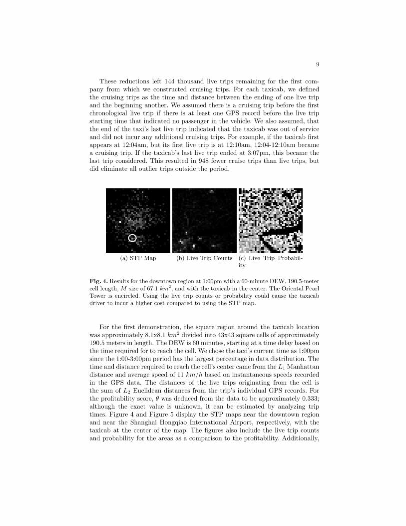
(a) STP Map (b) Live Trip Counts (c) Live Trip Probabil-ity

Fig. 4. Results for the downtown region at 1:00pm with a 60-minute DEW, 190.5-metercell length, M size of 67.1 km2, and with the taxicab in the center. The Oriental PearlTower is encircled. Using the live trip counts or probability could cause the taxicabdriver to incur a higher cost compared to using the STP map.

For the first demonstration, the square region around the taxicab locationwas approximately 8.1x8.1 km2 divided into 43x43 square cells of approximately190.5 meters in length. The DEW is 60 minutes, starting at a time delay based onthe time required for to reach the cell. We chose the taxi’s current time as 1:00pmsince the 1:00-3:00pm period has the largest percentage in data distribution. Thetime and distance required to reach the cell’s center came from the L1 Manhattandistance and average speed of 11 km/h based on instantaneous speeds recordedin the GPS data. The distances of the live trips originating from the cell isthe sum of L2 Euclidean distances from the trip’s individual GPS records. Forthe profitability score, θ was deduced from the data to be approximately 0.333;although the exact value is unknown, it can be estimated by analyzing triptimes. Figure 4 and Figure 5 display the STP maps near the downtown regionand near the Shanghai Hongqiao International Airport, respectively, with thetaxicab at the center of the map. The figures also include the live trip countsand probability for the areas as a comparison to the profitability. Additionally,

10

(a) STP Map (b) Live Trip Counts (c) Live Trip Probabil-ity

Fig. 5. Results for the Shanghai International Airport region at 1:00pm with a 60-minute DEW, 190.5-meter cell length, M size of 67.1 km2, and with the taxicab in thecenter. The airport terminal is encircled. The high count of live trips from the terminalshadows the other locations, hiding other potentially profitable locations that our STPmap captures.

(a) STP Map 1 (b) STP Map 2

Fig. 6. Results for overlapping downtown regions at 1:00pm with a 60-minute DEW,90.5-meter cell length, M size of 67.1 km2, and with the taxicab in the center. Thetop-right quadrant of STP Map 1 overlaps the bottom-left quadrant of STP Map 2.There is a clear difference between the overlapped regions as lower profitability areasin one are often higher profitability areas in the other.

Fig. 7. Color scale from low to high values for Figures 4, 5, and 6.

to show that two taxicabs at the same time get two distinct STP maps, Figure6 shows two overlapping regions in which the top-right quadrant of Figure 6(a)overlaps the bottom-left quadrant of Figure 6(b). For visualization purposes,negative profitability areas are set to zero to highlight the profitable regions,which are of interest to the taxi driver.

Figure 8 overlays the STP map in Figure 4(a) with the downtown area usingGoogle Earth and one-hour DEW. The results show a correlation with office

11

Fig. 8. Results for the downtown region STP map over laid with the Google Earth’ssatellite image at 1:00pm, a 60-minute DEW, 190.5 meters cell length, and M size of67.1 km2. Lighter areas represent higher profitability scores and often correlate withareas expected to be profitable, such as the Shanghai International Convention Center.

buildings and the STP map. There are two issues to note. First, Google Earthdistorts the cell edges in an effort to stretch the image over the area, leading topotential misinterpretation, although minor. Second, the cell granularity playsan important role in the results. Near the image center, the construction areanear the Grand Hyatt Hotel shows high profitability while the Grand Hyattitself does not show as high profitability as would be expected. This is becausethe cell boundary between these locations is splitting the trips between them.While this is an issue, it is more typical for a group of close cells to have similarprofitability scores. From the viewpoint of a taxicab driver, this is not an issuebecause the goal to find general locations of high profitability, not necessarilythe specific 190.5 by 190.5 square meters. Figure 9 similarly shows an STP mapoverlaying the airport. The airport is one of the hottest locations, producingnumerous profitable trips that make it a favorite location among taxi drivers. Inthis case, the entire terminal area has similar profitability even though the cellsmaybe splitting the activity among them. A graphical glitch is preventing thered cell from completely showing near the image center.

5 Validation

To validate this method, we must show that the STP maps correlate with actualprofitability. If assumed that taxicab drivers move towards high profitable areaswhen cruising, then it is logical that the ending location of a cruising trip (i.e.,

12

Fig. 9. Results for the Shanghai International Airport region STP map over laid withthe Google Earth’s satellite image at 1:00pm, a 60-minute DEW, 190.5 meters celllength, and M size of 67.1 km2. Lighter areas represent higher profitability scores andcorrelates with airport terminal and surrounding area. Note that a graphical glitch iscausing the red center cell to be distorted.

the beginning location of a live trip) is a profitable location. If these endinglocations correlate to the higher profitable areas in the STP maps generated forthe taxicab throughout the day, and this correlates with known taxi profitability,then the STP map correctly suggests good locations. In other words, if theaggregate profitability scores associated with the ending locations of cruise tripsthroughout the day correlates to actual profitability, which can be determinedby live time to total time for a taxi, then the correlation should be positive.

We selected five distinct test sets of 600 taxicabs and removed taxis with lessthan 19 total trips to focus on those that covered the majority of the day. Thisresulted in 516-539 taxis per test set. For each taxicab, we followed their pathof live and cruising trips throughout the day. When a taxicab switched from liveto cruising, we generated an STP map using a 15-minute DEW for a 15.8 by15.8 km2 area divided into 167 by 167-square cells (approximately 95 metersin length) with the taxi at the center. We summed the profitability scores atcruising trip ending locations and correlated them with the real live time to totaltime ratio that defines actual profitability. We then repeated the experiment,increasing the cell size and DEW while holding the region size constant.

13

Fig. 10. The total and cruise trips for one dataset with 538 taxis, sorted by total time.Increasing the total time tends to disproportionately increase the count of cruise tripsto live trips.

Fig. 11. The total, live, and cruise times in seconds for one dataset with 538 taxis,sorted by total time. The amount of cruising time is often greater than live time.

Figures 10, 11, and 12 visualize typical characteristics of the test sets. Figure10 shows trip counts and Figure 11 shows trip times with taxis sorted by totaltime. There is a distinct group having higher total times, but this results froma larger percent of cruising time relative to the other taxis. Comparing thiswith Figure 12, the taxicab profits with taxis sorted by total time, reveals thatthe total time in service does not necessarily improve profits; in fact, it has atendency to have the opposite effect. Figure 12 also shows that an increase intotal time typically yields more trips, but does not necessarily increase overallprofits.

14

Fig. 12. The profit (live time/total time) for one dataset with 538 taxis, sorted by totaltime. There is a slight upward trend in profits as the total time decreases, indicatingthat an increase in total time does not guarantee an increase in profit.

Figure 13 displays the resulting average correlation over the datasets forthree cell sizes and DEWs. The average correlations approached 0.50 with aslightly higher median. The trend in correlation clearly demonstrates the effectof cell sizes. Small sizes do not accurately represent the profitability and largersizes tend to distort. Additionally, the DEW shows a definite trend. The morehistorical data, the better the correlation; however, caution should be taken.Increasing the DEW increases the amount of historical data, but may cause it toinclude data not representative of the current period. For example, if the DEWincludes both rush hour and non-rush hour traffic, then the profitability maynot reflect real profitability. In addition, if a taxi only cruises for a few minutes,the extra 50 minutes of a 60-minute DEW has less importance in making adecision. Figure 14 confirms this hypothesis—holding the 190x190 m2 cell sizeconstant, the correlation increases with the increasing DEW until past the 90-minute mark. Since the DEW starts at 1:00pm but was time delayed as describedin the method, it started including the traffic pattern beyond the afternoon rushhour but before the evening rush hour.

The positive correlation was not as high as expected, but investigating thescatter plots revealed that there is a good correlation. As an example, Figure 15shows the scatter plot correlation for one test set with a 30-minute DEW anda 190x190 m2 cell size. The Hit Profit is the sum of all profit scores from cellswhere the taxicab ended a cruising trip and the Live Time/Total Time is theprofitability of the taxicab for that day. As indicated by the trend line, the higherthe taxicab profitability, the higher the Hit Profit. While the correlation for thisspecific set was 0.51, there is a definite upward trend in correlation among allsets with the majority of taxis are ending cruise trips in the higher profitablelocations based on our method.

15

Fig. 13. Average correlation of the five test datasets for a given cell size and DEW.The cell size 190x190 m2 produced the best overall correlation, reaching 0.51 for oneof the five datasets.

Fig. 14. Correlations values for the 190x190 m2 cell size with varying DEW size start-ing at 1:00pm. A DEW size greater than 90 minutes causes a significant decrease incorrelation, demonstrating it’s importance.

16

Fig. 15. An example of correlation results with an × marker indicating a taxicab.This test set used a cell size 190x190 m2 with a 30-minute DEW. The Hit Profit isthe sum of all profit scores from cells where the taxicab ended a cruising trip and theLive Time/Total Time is the profitability of the taxicab for that day. The majority oftaxicabs are ending in the more profitable locations, providing a positive correlationbetween the STP map and actual profitability as shown by the upward trend line.

6 Future Work

There are several potential improvements for this method. First, we did notfocus on the temporal aspect beyond shifting the DEW at a delayed time andadjusting the size. Patterns in time may affect results by allowing it to includedata from two distinct periods in relation to the traffic pattern; for example,rush hour traffic data included with non-rush hour data. To a lesser extent, thecell sizes and region M may need to adjust with time as well; for example, late atnight, there may be a need to increase the cell size due to lower probability of livetrips and an increase in M to include more potential locations. For validationpurposes, M was large enough to ensure that all cruising trips considered endedwithin the area with our profitability scores; otherwise, the score would be zerowhen in reality it should be positive or negative. The goal would be to developa dynamic STP mapping system that adjusts each of these components givencurrent conditions and time.

Another improvement involves the distance calculations. The L1 Manhattandistance formula determined the distance between the current taxi location andthe location of interest. While this is more realistic than using the L2 Euclideandistance, it relies on a grid city model, which is not always applicable to all

17

areas of the city. The live trip distances used the L2 Euclidean distance betweenindividual GPS records to determine total distance, which has an associatederror in accuracy as well. These calculations also did not consider obstacles;for example, drivers must cross rivers at bridges or tunnels, which may adddistance and time to a trip. One potential solution is to use the road network,current traffic conditions, and known obstacles to find the best path to a locationand then use the path to determine profitability. An alternative is to capturethe driver’s intuitive nature to find the best path or to use distances of commonpaths traveled by multiple taxis. A preliminary investigation into this alternativerevealed that it is a possibility given enough GPS records.

Since the ultimate goal is for a taxi driver to use the STP map, the systemneeds to be real-time and use visuals that are easy to understand and not dis-tractive to driving. It could also take into consideration the current traffic flowto determine a more accurate profitability score, and give higher potential prof-itability path suggestions leading to a profitable location. This could increasethe probability of picking up a passenger before reaching the suggested locationand thereby further reduce cruise time and increase profits.

7 Conclusion

The growing demand for public transportation and decreasing budgets haveplaced emphasis on increasing taxicab profitability. Research in this area hasfocused on improving service through taxi routing techniques and balancing sup-ply and demand. Realistically, cruising taxicabs do not easily lend themselves torouting because of the nature of the service and the driver’s desire for short-termprofitability. Since the live and cruising times define the overall profitability, anda taxicab may spend 35-60 percent of time cruising, the goal is reducing cruisetime while increasing live time. Our framework potentially improves profitabilityby offering location suggestions to taxicab drivers, based on profitability infor-mation using historical GPS data, which can reduce overall cruising time. Themethod uses spatial and temporal data to generate a location suggesting STPmap at the beginning of a cruise trip based on a profitability score defined bythe live time to total time profitability definition. A case study of Shanghai taxiservice demonstrates our method and shows the potential for increasing profitswhile decreasing cruise times. The correlation results between our method andactual profitability shows a promising positive correlation and potential for fu-ture work in increasing taxicab profitability.

References

1. Schaller Consulting: The New York City Taxicab Fact Book, Schaller Consulting,Brooklyn, NY, 2006, available at http://www.schallerconsult.com/taxi/taxifb.pdf

2. Yamamoto, K., Uesugi, K., and Watanabe, T.: Adaptive Routing of Cruising Taxisby Mutual Exchange of Pathways, Knowledge-Based Intelligent Information andEngineering Systems, 5178 (2008) 559–566

18

3. Li, Q., Zeng Z., Bisheng, Y., and Zhang, T.: Hierarchical route planning based ontaxi GPS-trajectories, 17th International Conference on Geoinformatics (Fairfax,2009), pp. 1–5

4. Wang, H.: The Strategy of Utilizing Taxi Empty Cruise Time to Solve the ShortDistance Trip Problem, Masters Thesis, The University of Melbourne, 2009

5. Cheng, S. and Qu, X.: A service choice model for optimizing taxi service delivery,12th International IEEE Conference on Intelligent Transportation Systems, ITSC’09 (St. Louis, 2009), pp. 1–6

6. Phithakkitnukoon, S., Veloso, M., Bento, C., Biderman, A., and Ratti, C.: Taxi-aware map: identifying and predicting vacant taxis in the city, Proceedings of theFirst international joint conference on Ambient intelligence, AmI’10 (Malaga, 2010),pp. 86–95

7. Hong-Cheng, G., Xin, Y., and Qing, W.: Investigating the effect of travel time vari-ability on drivers’ route choice decisions in Shanghai, China, Transportation Plan-ning and Technology, 33 (2010) 657–669

8. Li, Y., Miller, M.A., and Cassidy, M.J., Improving Mobility Through Enhanced Tran-sit Services: Transit Taxi Service for Areas with Low Passenger Demand Density,University of California, Berkeley and California Department of Transportation,2009.

9. Cooper, J., Farrell, S., and Simpson, P.: Identifying Demand and Optimal Locationfor Taxi Ranks in a Liberalized Market, Transportation Research Board 89th AnnualMeeting (2010)

10. Sirisoma, R.M.N.T., Wong, S.C., Lam, W.H.K., Wang, D., Yan, H., and Zhang, P.:Empirical evidence for taxi customer-search model, Transportation Research Board88th Annual Meeting, 163 (2009) 203–210

11. Yang, H., Fung, C.S., Wong, K.I., Wong, S.C.: Nonlinear pricing of taxi services,Transportation Research Part A: Policy and Practice, 44 (2010) 337–348

12. Chintakayala, P., and Maitra, B., Modeling Generalized Cost of Travel and ItsApplication for Improvement of Taxies in Kolkata, Journal of Urban Planning andDevelopment, 136 (2010) 42–49

13. Wikipedia, Shanghai — Wikipedia, The Free En-cyclopedia, 2011, Online; accessed 21-May-2011,http://en.wikipedia.org/w/index.php?title=Shanghai&oldid=412823222

14. TravelChinaGuide.com, Get Around Shanghai by Taxi, Shang-hai Transportation, 2011, Online; accessed 9-February-2011,http://www.travelchinaguide.com/cityguides/shanghai/transportation/taxi.htm

15. Shanghai Taxi Cab Rates and Companies, Kuber, 2011, Online; accessed 9-February-2011, http://kuber.appspot.com/taxi/rate

16. Yuan, Jing and Zheng, Yu and Zhang, Chengyang and Xie, Wenlei and Xie, Xingand Sun, Guangzhong and Huang, Yan, T-drive: driving directions based on taxitrajectories, Proceedings of the 18th SIGSPATIAL International Conference on Ad-vances in Geographic Information Systems, GIS ’10 (San Jose, 2010), pp. 99–108

17. Ge, Yong and Xiong, Hui and Tuzhilin, Alexander and Xiao, Keli and Gruteser,Marco and Pazzani, Michael, An energy-efficient mobile recommender system, Pro-ceedings of the 16th ACM SIGKDD international conference on Knowledge discov-ery and data mining, KDD ’10 (Washington, DC, 2010), pp. 899–908