
Towards numerical modelling of natural subduction systems
162
UTRECHT STUDIES IN EARTH SCIENCES 185 Towards numerical modelling of natural subduction systems With an application to Eastern Caribbean subduction M.R.T. Fraters
Transcript of Towards numerical modelling of natural subduction systems

UTRECHT STUDIES IN EARTH SCIENCES
Utrecht UniversityFaculty of GeosciencesDepartment of Earth Sciences
185ISSN 2211-4335
US
ES
18
5M
.R.T. Fraters – To
ward
s nu
merical m
od
elling
of n
atural su
bd
uctio
n system
s
Towards numerical modelling of natural subduction systems
With an application toEastern Caribbean subduction
M.R.T. Fraters
USES185-cover-Fraters.indd 1 03-04-19 07:28


530578-L-sub01-bw-Fraters530578-L-sub01-bw-Fraters530578-L-sub01-bw-Fraters530578-L-sub01-bw-FratersProcessed on: 10-4-2019Processed on: 10-4-2019Processed on: 10-4-2019Processed on: 10-4-2019 PDF page: 1PDF page: 1PDF page: 1PDF page: 1
Towards numerical modelling of naturalsubduction systems with an application to
Eastern Caribbean subduction
Menno R. T. Fraters
UTRECHT STUDIES IN EARTH SCIENCES
No. 185

530578-L-sub01-bw-Fraters530578-L-sub01-bw-Fraters530578-L-sub01-bw-Fraters530578-L-sub01-bw-FratersProcessed on: 10-4-2019Processed on: 10-4-2019Processed on: 10-4-2019Processed on: 10-4-2019 PDF page: 2PDF page: 2PDF page: 2PDF page: 2
Members of the dissertation committee:
Prof. Dr. Magali BillenDept of Earth & Planetary SciencesUC Davis, USA
Prof. Dr. Nicolas ColticeDépartement de GéosciencesEcole Normale Supérieure de Paris, France
Prof. Dr. Clint ConradCentre for Earth Evolution and Dynamics (CEED)Department of GeosciencesUniversity of Oslo, Norway
Prof. Dr. Boris KausInstitute of GeosciencesJohannes Gutenberg University Mainz, Germany
Prof. Dr. Wouter SchellartFaculty of Science, Geology and GeochemistryVrije Universiteit Amsterdam, Netherlands
Copyright © 2019 Menno Fraters, Utrecht UniversityAll rights reserved. No part of this publication may be reproduced in any form,by print or photographic print, microfilm or any other means, without writtenpermission by the author.Printed in the Netherlands by Ipskamp Printing, Enschede
ISBN: 978-90-6266-540-2
530578-L-sub01-bw-Fraters530578-L-sub01-bw-Fraters530578-L-sub01-bw-Fraters530578-L-sub01-bw-FratersProcessed on: 10-4-2019Processed on: 10-4-2019Processed on: 10-4-2019Processed on: 10-4-2019 PDF page: 3PDF page: 3PDF page: 3PDF page: 3
Towards numerical modelling ofnatural subduction systems with an
application to Eastern Caribbeansubduction
Een opstap naar numerieke modellering van natuurlijke subductiesystemen met een toepassing op het oostlijke Caribisch gebied
(met een samenvatting in het Nederlands)
Proefschriftter verkrijging van de graad van doctor
aan de Universiteit Utrechtop gezag van de rector magnificus, prof.dr. H. R. B. M. Kummeling,
ingevolge het besluit van het college voor promotiesin het openbaar te verdedigen op
woensdag 15 mei 2019 des ochtends te 10.30 uur
door
Menno Roeland Theodorus Fratersgeboren op 3 oktober 1989 te Wageningen

530578-L-sub01-bw-Fraters530578-L-sub01-bw-Fraters530578-L-sub01-bw-Fraters530578-L-sub01-bw-FratersProcessed on: 10-4-2019Processed on: 10-4-2019Processed on: 10-4-2019Processed on: 10-4-2019 PDF page: 4PDF page: 4PDF page: 4PDF page: 4
Promotoren:Prof. dr. W. SpakmanProf. dr. D.J.J van HinsbergenProf. dr. W. Bangerth
Copromotor:Dr. C.A.P. Thieulot
This work is funded by the Netherlands Organization for Scientific Research (NWO),
as part of the Caribbean Research program, grant 858.14.070. This work was partly
supported by the Research Council of Norway through its Centres of Excellence funding
scheme, project number 223272., the Netherlands Research Centre for Integrated Solid
Earth Science (ISES), the Computational Infrastructure in Geodynamics initiative (CIG),
through the National Science Foundation under Award No. EAR-0949446 and The
University of California - Davis, and by the National Science Foundation under awards
OCI-1148116 and OAC-1835673 as part of the Software Infrastructure for Sustained
Innovation (SI2) program (now the Cyberinfrastructure for Sustained Scientific
Innovation, CSSI).

530578-L-sub01-bw-Fraters530578-L-sub01-bw-Fraters530578-L-sub01-bw-Fraters530578-L-sub01-bw-FratersProcessed on: 10-4-2019Processed on: 10-4-2019Processed on: 10-4-2019Processed on: 10-4-2019 PDF page: 5PDF page: 5PDF page: 5PDF page: 5
Il est encore plus facile de juger de l’esprit d’un hommepar ses questions que par ses réponses.
It is easier to judge the mind of a man by his questionsthan his answers.
Pierre-Marc-Gaston de Lévis
Maximes, préceptes et réflexions sur différens sujetsde morale et de politique. Paris (1808), Maxim xviii

530578-L-sub01-bw-Fraters530578-L-sub01-bw-Fraters530578-L-sub01-bw-Fraters530578-L-sub01-bw-FratersProcessed on: 10-4-2019Processed on: 10-4-2019Processed on: 10-4-2019Processed on: 10-4-2019 PDF page: 6PDF page: 6PDF page: 6PDF page: 6

530578-L-sub01-bw-Fraters530578-L-sub01-bw-Fraters530578-L-sub01-bw-Fraters530578-L-sub01-bw-FratersProcessed on: 10-4-2019Processed on: 10-4-2019Processed on: 10-4-2019Processed on: 10-4-2019 PDF page: 7PDF page: 7PDF page: 7PDF page: 7
Contents
Contents vii
1 Introduction 1
2 Efficient and Practical Newton Solvers for Nonlinear Stokes Systemsin Geodynamic Problems 72.1 Summary . . . . . . . . . . . . . . . . . . . . . . . . . . . . . . . . . 82.2 Introduction . . . . . . . . . . . . . . . . . . . . . . . . . . . . . . . 82.3 Problem statement and numerical methods . . . . . . . . . . . . 11
2.3.1 The model . . . . . . . . . . . . . . . . . . . . . . . . . . . . 112.3.2 Discretization . . . . . . . . . . . . . . . . . . . . . . . . . . 132.3.3 Newton linearization . . . . . . . . . . . . . . . . . . . . . 142.3.4 Restoring symmetry of Juu . . . . . . . . . . . . . . . . . . 162.3.5 Restoring well-posedness of the Newton step . . . . . . . 182.3.6 Algorithms for the solution of the nonlinear problem . . 22
2.4 Numerical experiments using common benchmarks . . . . . . . 262.4.1 Nonlinear channel flow . . . . . . . . . . . . . . . . . . . . 262.4.2 Spiegelman et al. benchmark . . . . . . . . . . . . . . . . . 282.4.3 Tosi et al. benchmark . . . . . . . . . . . . . . . . . . . . . 332.4.4 A 3d subduction test case . . . . . . . . . . . . . . . . . . . 34
2.5 Conclusions . . . . . . . . . . . . . . . . . . . . . . . . . . . . . . . 402.6 Acknowledgments . . . . . . . . . . . . . . . . . . . . . . . . . . . . 412.7 Appendix A: The connection between elliptic operators, well-posedness
of the Newton update equation, and eigenvalues of coefficients . 412.8 Appendix B: A look at some common rheologies . . . . . . . . . . 42
2.8.1 Power law rheology . . . . . . . . . . . . . . . . . . . . . . 432.8.2 Drucker-Prager rheology . . . . . . . . . . . . . . . . . . . 442.8.3 The rheology of the Spiegelman et al. benchmark . . . . . 45
vii

530578-L-sub01-bw-Fraters530578-L-sub01-bw-Fraters530578-L-sub01-bw-Fraters530578-L-sub01-bw-FratersProcessed on: 10-4-2019Processed on: 10-4-2019Processed on: 10-4-2019Processed on: 10-4-2019 PDF page: 8PDF page: 8PDF page: 8PDF page: 8
2.8.4 The rheology of the Tosi et al. benchmark . . . . . . . . . 462.9 Appendix C: Parameters for the 3d subduction test case . . . . . . 46
3 The Geodynamic World Builder: a solution for complex initial con-ditions in numerical modelling 493.1 Abstract . . . . . . . . . . . . . . . . . . . . . . . . . . . . . . . . . . 503.2 Introduction . . . . . . . . . . . . . . . . . . . . . . . . . . . . . . . 503.3 Geodynamic World Builder Philosophy . . . . . . . . . . . . . . . 51
3.3.1 User Philosophy . . . . . . . . . . . . . . . . . . . . . . . . 513.3.2 Code philosophy . . . . . . . . . . . . . . . . . . . . . . . . 53
3.4 Using the World Builder . . . . . . . . . . . . . . . . . . . . . . . . 543.4.1 Standalone examples . . . . . . . . . . . . . . . . . . . . . 553.4.2 Using the GWB with SEPRAN . . . . . . . . . . . . . . . . . 583.4.3 Using the GWB with ELEFANT . . . . . . . . . . . . . . . . 593.4.4 Using the GWB with ASPECT . . . . . . . . . . . . . . . . . 593.4.5 Performance . . . . . . . . . . . . . . . . . . . . . . . . . . 64
3.5 Discussion . . . . . . . . . . . . . . . . . . . . . . . . . . . . . . . . 643.6 Code availability . . . . . . . . . . . . . . . . . . . . . . . . . . . . . 643.7 Acknowledgements . . . . . . . . . . . . . . . . . . . . . . . . . . . 653.8 2D subduction examples . . . . . . . . . . . . . . . . . . . . . . . . 65
3.8.1 Cartesian input file . . . . . . . . . . . . . . . . . . . . . . 653.8.2 Spherical input file . . . . . . . . . . . . . . . . . . . . . . 66
3.9 3D ocean spreading example input file . . . . . . . . . . . . . . . 683.10 3D subduction example input file . . . . . . . . . . . . . . . . . . 683.11 SEPRAN 2D subduction . . . . . . . . . . . . . . . . . . . . . . . . . 703.12 ELEFANT 3D Double subduction setup . . . . . . . . . . . . . . . 723.13 ASPECT 3d curved subduction . . . . . . . . . . . . . . . . . . . . 73
4 Assessing the geodynamics of strongly arcuate subduction zones: theeastern Caribbean subduction setting. 754.1 Summary . . . . . . . . . . . . . . . . . . . . . . . . . . . . . . . . . 764.2 Introduction . . . . . . . . . . . . . . . . . . . . . . . . . . . . . . . 764.3 Three-dimensional initial model of arcuate subduction based on
the tectonic setting of the Lesser Antilles slab . . . . . . . . . . . . 794.4 Model setup . . . . . . . . . . . . . . . . . . . . . . . . . . . . . . . 84
4.4.1 Numerical model setup . . . . . . . . . . . . . . . . . . . . 844.4.2 Boundary conditions . . . . . . . . . . . . . . . . . . . . . 864.4.3 Rheological model . . . . . . . . . . . . . . . . . . . . . . . 86
4.5 Experiments . . . . . . . . . . . . . . . . . . . . . . . . . . . . . . . 90

530578-L-sub01-bw-Fraters530578-L-sub01-bw-Fraters530578-L-sub01-bw-Fraters530578-L-sub01-bw-FratersProcessed on: 10-4-2019Processed on: 10-4-2019Processed on: 10-4-2019Processed on: 10-4-2019 PDF page: 9PDF page: 9PDF page: 9PDF page: 9
4.5.1 The reference model . . . . . . . . . . . . . . . . . . . . . . 904.5.2 The influence of the crustal rheology of the subducting
plate . . . . . . . . . . . . . . . . . . . . . . . . . . . . . . . 964.5.3 The influence of mantle viscosity and the temperature of
the slab . . . . . . . . . . . . . . . . . . . . . . . . . . . . . . 974.5.4 The influence of vertical weak zones in the slab . . . . . . 1024.5.5 The influence of the subducting plate velocity . . . . . . . 104
4.6 Discussion and conclusions . . . . . . . . . . . . . . . . . . . . . . 1074.7 Appendix A: GWB input . . . . . . . . . . . . . . . . . . . . . . . . . 1104.8 Appendix B: ASPECT intput . . . . . . . . . . . . . . . . . . . . . . 113
5 Conclusions and outlook 119
Bibliography 123
Summary 135
Samenvatting 137
Acknowledgements 139
Funding 143
Curriculum Vitae 145

530578-L-sub01-bw-Fraters530578-L-sub01-bw-Fraters530578-L-sub01-bw-Fraters530578-L-sub01-bw-FratersProcessed on: 10-4-2019Processed on: 10-4-2019Processed on: 10-4-2019Processed on: 10-4-2019 PDF page: 10PDF page: 10PDF page: 10PDF page: 10

530578-L-sub01-bw-Fraters530578-L-sub01-bw-Fraters530578-L-sub01-bw-Fraters530578-L-sub01-bw-FratersProcessed on: 10-4-2019Processed on: 10-4-2019Processed on: 10-4-2019Processed on: 10-4-2019 PDF page: 11PDF page: 11PDF page: 11PDF page: 11
1Introduction
530578-L-sub01-bw-Fraters530578-L-sub01-bw-Fraters530578-L-sub01-bw-Fraters530578-L-sub01-bw-FratersProcessed on: 10-4-2019Processed on: 10-4-2019Processed on: 10-4-2019Processed on: 10-4-2019 PDF page: 12PDF page: 12PDF page: 12PDF page: 12
1
Chapter 1. Introduction
It has long been understood that there is a strong coupling between pro-cesses of Earth’s mantle and the tectonic evolution but the nature of the dy-namic processes involved and their interaction continues to be a main topicin geodynamic research. Sub-disciplines of Solid Earth Science, like geology orseismology, provide various valuable observations of the internal workings ofour planet but usually provide only indirect information on acting processes.Direct access to the operation of deep processes is provided by forward numer-ical modelling, solving the pertinent conservation laws of continuum mechan-ics, which ultimately may provide useful predictions of geological, seismolog-ical, or geodetic observations such that these are better understood and thathypotheses of acting mantle processes can be tested against observations.
My goal in this thesis is to make new steps toward assessing how man-tle processes operate and affect tectonic evolution, particularly, by creatingsteps toward numerically simulating natural plate boundary regions involv-ing lithosphere subduction. By far most of current 3D subduction modellingis of a strongly generic nature aimed at understanding the process and itsinteraction with the mantle but not so much on simulating natural subduc-tion in past or present. Subduction plate boundaries are simplified in initialmodels to straight subduction trenches and pure trench-perpendicular con-vergence instead of implementing the natural geometry of subduction zonesthat comprises highly variable trench geometry and the generally oblique con-vergence of the subducting plate towards the trench. Also, often simplified lin-ear material-rheology is used. Of course, there are several reasons why thischaracterizes the current stage of 3D subduction modelling. Some of theseare: subduction in 3D space is a complex process that requires step-by-stepinvestigation; obtaining a feasible computation time; exploiting the possibil-ity to use simple free-slip and no-slip boundaries along the side-walls of themodel domain; or the practical difficulty of constructing 3-D initial models thatmimic the geometrical complexity of natural subduction in an embryonic, oradvanced stage of evolution.
In this thesis, I aim to address the research problems of 1) decreasing thecomputation time, while improving the accuracy, of subduction modelling in-volving realistic non-linear material models, here visco-plasticity, and more ad-vanced boundary conditions, of 2) establishing a versatile method for build-ing complex 3D geodynamic models of subduction for use as initial conditionof subduction modelling, and 3) the research problem of the geodynamics ofstrongly arcuate subduction. Addressing the latter research problem builds onproviding solutions to the first problems and is intended as a showcase of the
2

530578-L-sub01-bw-Fraters530578-L-sub01-bw-Fraters530578-L-sub01-bw-Fraters530578-L-sub01-bw-FratersProcessed on: 10-4-2019Processed on: 10-4-2019Processed on: 10-4-2019Processed on: 10-4-2019 PDF page: 13PDF page: 13PDF page: 13PDF page: 13
1
practical feasibility of coming much closer to simulating natural evolution inall its geometrical complexity.
Chapter 2 is devoted to providing a solution to the first research problem.Depending on ambient temperature and pressure, mantle materials exhibit of-ten a nonlinear response of strain-rate to deforming stress. Using nonlinearrheology causes the Stokes equation, describing the force balance, to becomenonlinear which consequently leads in Finite Element as well as Finite Differ-ence applications to a system of nonlinear equations to be resolved. The stan-dard and stable way to tackle the nonlinearity is by setting up, for each timestep, an iteration scheme by the Picard method which is robust and numer-ically the easiest way to solve the nonlinear system of equations. However,complex geodynamic problems, e.g., simulating natural mantle processes, arecharacterized by strong nonlinear viscosity and strain-rate variation of severalorders of magnitudes occurring over short distances, often causing the Picarditeration to slowly converge in each time step, i.e. considerably increasing theoverall computation time.
A more advanced method is the Newton method that uses informationabout the derivatives of the nonlinear equations. Under several conditions, thismethod can converge much faster to the correct solution of the nonlinear sys-tem of equations. However, the Newton method for the Stokes equations is notalways stable and may lead to systems of equations for which the linear solvercan not converge, because the involved matrix is singular. To develop a stableand (almost always) converging Newton method that also leads to a consider-able decrease in computation time, is the main goal of Chapter 2.
Chapter 3 tackles the second research problem of finding an effective andversatile method for constructing 3D geodynamic initial models that allow toapproximate the geometrical complexity of natural plate boundaries and 3Dsubduction. Setting up initial conditions for geodynamic models, especially in3D, is so far done by personally developed methods and code, which can bea very time-consuming process and so far has not led to a more general, easyto use, open-source solution accessible to the modelling community. Chap-ter 3 aims to offer exactly that versatile solution, called the Geodynamic WorldBuilder, such that it is not only relatively easy to use but also provides a simpleinterface for use with the various community, or personal, numerical modellingcodes.
Chapter 4 concerns the problem of the geodynamics involved in arcuatesubduction along strongly curved trenches. Trench curvature is still not wellunderstood but is a common characteristic of natural subduction zones across
3

530578-L-sub01-bw-Fraters530578-L-sub01-bw-Fraters530578-L-sub01-bw-Fraters530578-L-sub01-bw-FratersProcessed on: 10-4-2019Processed on: 10-4-2019Processed on: 10-4-2019Processed on: 10-4-2019 PDF page: 14PDF page: 14PDF page: 14PDF page: 14
1
Chapter 1. Introduction
the globe. The negative buoyancy of the subducting slab exerts a vertical forceon the lithosphere entering the trench, slab pull, that basically acts trench-perpendicular but still has an arc-forming potential by its interaction with lat-eral lithosphere heterogeneity and with slab-induced mantle flow. Slab pull,however, cannot easily explain the generally observed trench-oblique conver-gence of tectonic plates along strongly arcuate trenches. Particularly, arcuatesubduction systems, such as the Marianas-Izu-Bonin, or Aleutians-Alaska sys-tems, are characterized by trench-perpendicular convergence at one trenchsegment (Marianas, Alaska) while a strong trench-parallel component of sub-ducting plate motion occurs elsewhere along the trench. This suggest thatthe slab subducting at the latter trench segment may be involved in lateraltransport through the mantle. In Chapter 4, I investigate this possible geody-namic aspect of arcuate subduction for the Lesser Antilles system of the easternCaribbean where near trench-parallel westward subducting plate motion oc-curs along the northern trench below which a south-dipping slab is observedby seismic tomography. This application to a geometrically complex naturalsubduction system showcases the benefits of the Newton method developed inChapter 2, i.e. stable and fast convergence, and the benefits of the GeodynamicWorld Builder for setting up an application to natural subduction. It also in-tends to demonstrate that more detailed and elaborate applications to naturalsubduction systems are now within reach.
A common thread across all chapters is the use and development of theASPECT code, which I would like to introduce here. ASPECT (short for Ad-vanced Solver for Problems in Earth’s ConvecTion) is a modern C++ code de-signed to solve the equations underpinning the geodynamic processes of thecrust-mantle system (Kronbichler et al., 2012; Heister et al., 2017). Althoughoriginally designed to model convection related problems, its modular designhas allowed a growing core of developers and users that have quickly expandedASPECT’s range of applications to thermo-mechanical modelling of the crust-mantle system using visco-plastic rheology (Glerum et al., 2018), free surface(Rose et al., 2017), melt transport (Dannberg and Heister, 2016; Dannberg andGassmöller, 2018), or even grain size evolution (Dannberg et al., 2017). AS-PECT is hosted by the Computational Infrastructure for Geodynamics1 (CIG).The code is based on the deal.II Finite Element library2 (Bangerth et al., 2007;
1www.geodynamics.org2https://www.dealii.org/
4

530578-L-sub01-bw-Fraters530578-L-sub01-bw-Fraters530578-L-sub01-bw-Fraters530578-L-sub01-bw-FratersProcessed on: 10-4-2019Processed on: 10-4-2019Processed on: 10-4-2019Processed on: 10-4-2019 PDF page: 15PDF page: 15PDF page: 15PDF page: 15
Alzetta et al., 2018) and employs numerical methods which are at the fore-front of research, such as adaptive mesh refinement (AMR) based on the p4estlibrary3 (Burstedde et al., 2011), linear and nonlinear solvers from Trilinos4
(Heroux and Willenbring, 2012), and stabilization of transport-dominated pro-cesses (Guermond et al., 2010, 2011). It also allows for various domain geome-tries, such as 2D and 3D Cartesian, 2D Cylindrical, and 3D Spherical domainsencompassing the entire crust-mantle system or parts of it, (hollow) spheresand even (parts of) ellipsoidal meshes. From the start, the code has been de-signed to support high levels of parallelism and has been run and shown toscale on up to tens of thousands of cores. The current version is hosted onthe github platform5 while stable releases are also available on the CIG web-site6. The code comes with an embedded and automatically generated manualwhich is extensive and up-to-date. Users are encouraged to get involved and tosubmit either code or so-called cookbooks (geodynamically relevant examplecases) which are thoroughly reviewed by core developers before being mergedinto the main version. Finally, every change to the code is tested before be-coming part of the main code by more than 600 integration tests (and growing)and more than 100 unit tests assertions (and growing) on a dedicated serverto ensure that none of the existing features of the code is ever broken, therebyensuring backwards compatibility.
My own investments in the development of ASPECT have provided me withthe advanced research modelling tool that constitutes the solid base of the re-search describe in my thesis.
3http://www.p4est.org/4http://trilinos.org/5https://github.com/geodynamics/aspect6https://aspect.geodynamics.org/
5

530578-L-sub01-bw-Fraters530578-L-sub01-bw-Fraters530578-L-sub01-bw-Fraters530578-L-sub01-bw-FratersProcessed on: 10-4-2019Processed on: 10-4-2019Processed on: 10-4-2019Processed on: 10-4-2019 PDF page: 16PDF page: 16PDF page: 16PDF page: 16
530578-L-sub01-bw-Fraters530578-L-sub01-bw-Fraters530578-L-sub01-bw-Fraters530578-L-sub01-bw-FratersProcessed on: 10-4-2019Processed on: 10-4-2019Processed on: 10-4-2019Processed on: 10-4-2019 PDF page: 17PDF page: 17PDF page: 17PDF page: 17
2Efficient and Practical Newton Solvers forNonlinear Stokes Systems in GeodynamicProblems

530578-L-sub01-bw-Fraters530578-L-sub01-bw-Fraters530578-L-sub01-bw-Fraters530578-L-sub01-bw-FratersProcessed on: 10-4-2019Processed on: 10-4-2019Processed on: 10-4-2019Processed on: 10-4-2019 PDF page: 18PDF page: 18PDF page: 18PDF page: 18
2
Chapter 2. Efficient and Practical Newton Solvers for Nonlinear StokesSystems in Geodynamic Problems
2.1 SummaryMany problems in geodynamic modeling result in a nonlinear Stokes prob-
lem in which the viscosity depends on the strain rate and pressure (in additionto other variables). After discretization, the resulting nonlinear system is mostcommonly solved using a Picard fixed-point iteration. However, it is well un-derstood that Newton’s method – when augmented by globalization strategiesto ensure convergence even from points far from the solution – can be substan-tially more efficient and accurate than a Picard solver.
In this contribution, we evaluate how a straight-forward Newton methodmust be modified to allow for the kinds of rheologies common in geodynam-ics. Specifically, we show that the Newton step is not actually well-posed forstrain rate-weakening models without modifications to the Newton matrix. Wederive modifications that guarantee well-posedness and that also allow for ef-ficient solution strategies by ensuring that the top-left block of the Newton ma-trix is symmetric and positive definite. We demonstrate the applicability andrelevance of these modifications with a sequence of benchmarks and a test caseof realistic complexity.
2.2 IntroductionGeodynamics aims to understand the dynamics of processes in and on the
Earth on a wide range of spatial and temporal scales, typically by connectingphysical processes to geological observations through either analogue or nu-merical modeling. The physical basis of most numerical modeling codes inthe geodynamics community are continuum mechanics conservation laws formomentum, mass, and energy. A fundamental assumption that underlies mostmodels is that we can average over the small scales at which natural materialsexhibit heterogeneity, and that we can approximate the macroscopic materialproperties to obtain equations that are well understood.
When considering long enough time scales, the dynamics of the mantle –and, to some degree, the crust – can then be described as a slow-moving fluidthat is governed by the Stokes equations, together with advection-diffusionequations for the temperature, chemical compositions, and possibly other
This chapter is currently under review at Geophysical Journal International as Efficient andPractical Newton Solvers for Nonlinear Stokes Systems in Geodynamic Problems, M. Fraters, W.Bangerth, C. Thieulot and W. Spakman.
8

530578-L-sub01-bw-Fraters530578-L-sub01-bw-Fraters530578-L-sub01-bw-Fraters530578-L-sub01-bw-FratersProcessed on: 10-4-2019Processed on: 10-4-2019Processed on: 10-4-2019Processed on: 10-4-2019 PDF page: 19PDF page: 19PDF page: 19PDF page: 19
2
2.2. Introduction
quantities. In the case of the Stokes equations, the fluid’s effective viscosity willthen depend on the material’s temperature, pressure, composition, and possi-bly other factors such as mechanical stress. Rheology – the science of deter-mining how a material flows – is therefore of key importance to this approach.Unfortunately, the rheology of Earth materials over geological timescales is alsoone of the least constrained ingredients in modeling the physical processes ofthe solid Earth. For both philosophical and computational reasons, many stud-ies use linear rheologies (e.g. Baumann et al., 2014; Fritzell et al., 2016; Pusokand Kaus, 2015), i.e., a viscosity that may depend on the external temperatureand chemical composition, but not on the fluid variables velocity (or its deriva-tives, e.g., the strain rate) and pressure. However, experiments have shown thatthe rheology of Earth materials can behave in a very nonlinear way (Karato andWu, 1993). Specifically, in deformation regimes, the mechanical stress leads tomaterial weakening with increasing strain-rate and consequently an effectiveviscosity that is a decreasing function of the strain rate. Furthermore, manywidely used rheological models – in particular if they try to incorporate plasticeffects – include a pressure dependence of the viscosity. This nonlinearity ofthe rheology results in models best described by a nonlinear variation of theStokes equations. An additional source of nonlinearities arises from the factthat Earth materials are compressible, i.e., that their density depends on thepressure. Because there is no convenient way of solving this kind of nonlinearpartial differential equation exactly, it is important to develop numerical meth-ods that can discretize and iteratively resolve the nonlinearity in the equations.
A simple and frequently used way to solve such nonlinear problems is touse Picard iterations, a particular form of fixed point iterations (Kelly, 1995). Init, one computes the viscosity and density as a function of the previous itera-tion’s strain rate and pressure, solves for a new velocity and pressure field, andthen repeats the process. The Picard iteration owes its popularity to the factthat it is relatively easy to implement in codes that only support linear rheolo-gies because it only requires the repeated solution of linear problems. It is alsooften globally convergent, i.e., with sufficiently many iterations it is possible toapproximate the solution of the nonlinear problem regardless of the choice ofinitial guess. Consequently, it is the method that is likely used in the majorityof mantle convection papers that actually iteratively resolve the nonlinearityin each time step; most papers do not explicitly state so, but van Keken et al.(2008); Tosi et al. (2015); Buiter et al. (2016); Glerum et al. (2018) are some ex-amples.
On the other hand, Picard iterations are often slow to converge, requiring
9

530578-L-sub01-bw-Fraters530578-L-sub01-bw-Fraters530578-L-sub01-bw-Fraters530578-L-sub01-bw-FratersProcessed on: 10-4-2019Processed on: 10-4-2019Processed on: 10-4-2019Processed on: 10-4-2019 PDF page: 20PDF page: 20PDF page: 20PDF page: 20
2
Chapter 2. Efficient and Practical Newton Solvers for Nonlinear StokesSystems in Geodynamic Problems
dozens or hundreds of iterations for strongly nonlinear problems – somethingwe also observe in our results in Section 2.4. This slow convergence may makethe solution of nonlinear problems to high accuracy prohibitively expensive.Consequently, commonly used approaches to cope with the high computa-tional cost are, for example, limiting the allowed number of Picard iterationsper timestep (e.g. Lemiale et al., 2008), combining Picard iterations with smalltimesteps to ensure good starting guesses (e.g. Ruh et al., 2013), or other mostlyad hoc approaches. In practice, however, many studies do not adequately doc-ument the exact algorithm used and how this affects the accuracy of the solu-tions of the equations considered.
Here, we address the slow convergence of nonlinear solvers by replacingthe Picard solver by a Newton solver (Kelly, 1995). Previous applications ofNewton’s method to geodynamics problems can be found in May et al. (2015);Rudi et al. (2015); Kaus et al. (2016); Spiegelman et al. (2016). Newton’s methodpromises quadratic convergence towards the solution, compared to the linearconvergence of the Picard iteration, when the initial guess is close enough tothe solution of the nonlinear problem and therefore offers the prospect of vastlyfaster solution procedures. On the other hand, the implementation of Newton’smethod is substantially more involved than a Picard iteration. Furthermore,requiring an initial guess that is close enough to the exact solution is often im-practical, and may require running a number of initial Picard iterations beforestarting the Newton iteration.
In this paper we present the details of an improvement on the Newtonmethod for the nonlinear Stokes problem, and discuss an implementation ofthis improved Newton solver along with recommendations on how to use it.Specifically, and going beyond what is available in the literature, we will showthat a naive application of Newton’s method may break both the symmetry andthe positive definiteness of the elliptic part of the (linearized) Jacobian of theStokes operator. While the lack of symmetry is annoying from a practical per-spective because it makes the solution of the linear system associated with eachNewton step more complicated, a lack of positive definiteness implies that theNewton step is ill-posed and may not have a solution. We will analyze both ofthese issues in detail and propose modifications to the Newton equations thatretain the symmetry and restore the positive definiteness. We will also considerwhether there are special classes of material models where these modificationsare not necessary. Unfortunately, as we will show, many rheologies that havebeen used extensively in the literature do not fall into these classes; our meth-ods are therefore strict improvements over the current state-of-the-art and will
10

530578-L-sub01-bw-Fraters530578-L-sub01-bw-Fraters530578-L-sub01-bw-Fraters530578-L-sub01-bw-FratersProcessed on: 10-4-2019Processed on: 10-4-2019Processed on: 10-4-2019Processed on: 10-4-2019 PDF page: 21PDF page: 21PDF page: 21PDF page: 21
2
2.3. Problem statement and numerical methods
allow solving problems that were not previously solvable with an unmodifiedNewton method.
While there are previous reports on using a Newton method for Stokes prob-lems in geodynamics applications (see, for example, May et al. (2015); Rudiet al. (2015); Kaus et al. (2016); Spiegelman et al. (2016)), we will provide a morein-depth discussion of the mathematical properties of the operators and linearsystems associated with each Newton step. We will underpin our claims withnumerical experiments and demonstrate that the approach advocated hereinis, indeed, more efficient and robust than previous approaches. In particular,we will show that our implementation of the Newton solver significantly de-creases computational time for realistic problems, with greatly improved ac-curacy. Our implementation is available as open source as part of the ASPECTcode (Kronbichler et al., 2012; Heister et al., 2017), an open source geodynamicscommunity code.
The layout of the remainder of this paper is as follows: We will first describethe mathematical formulation of the nonlinear Stokes problem we considerhere, its discretization, and linearization in Section 2.3. This section also con-tains our main results on how the Newton method has to be modified (“stabi-lized”) in order to make it well-posed, as well as a discussion of practical aspectsof how this method can be embedded in efficient nonlinear and linear solvers.We then show how the above works in practice in Section 2.4, first using threeartificial test cases and then using a realistic application of modeling subduc-tion. We conclude in Section 2.5.
2.3 Problem statement and numerical methods2.3.1 The model
Let us begin by concisely stating the equations we want to solve herein. Weare concerned with modeling convection in the Earth mantle, a process that istypically described by a coupled system of differential equations. Under com-monly used assumptions – see for example Schubert et al. (2001) – typical mod-els include a Stokes-like, compressible fluid flow system for the velocity u andpressure p defined in the volume Ω⊂ Rd (where the space dimension d = 2 or3) under consideration,
−∇·[
2η
(ε(u)− 1
3(∇·u)I
)]+∇p = ρg in Ω, (2.1)
−∇· (ρu) = 0 in Ω, (2.2)
11

530578-L-sub01-bw-Fraters530578-L-sub01-bw-Fraters530578-L-sub01-bw-Fraters530578-L-sub01-bw-FratersProcessed on: 10-4-2019Processed on: 10-4-2019Processed on: 10-4-2019Processed on: 10-4-2019 PDF page: 22PDF page: 22PDF page: 22PDF page: 22
2
Chapter 2. Efficient and Practical Newton Solvers for Nonlinear StokesSystems in Geodynamic Problems
where η is the viscosity, ρ the density, g the gravity vector, ε(·) denotes the sym-metric gradient operator defined by ε(v) = 1
2 (∇v+∇vT), and I is the d×d identitymatrix. (The sign in (2.2) is chosen in this way because −∇· is the adjoint op-erator to the gradient in the first equation, leading to a symmetric system if thedensity is constant, as shown below.)
While these equations describe a compressible model, we will assume forthe purposes of this paper that the fluid is in fact incompressible, i.e., that∇ · (ρu) = ρ∇ ·u = 0. We do so because we can illustrate all difficulties asso-ciated with the Newton method using this simplification already, and becausemany of the approximations used in geodynamics (for example, the Boussi-nesq approximation) also assume incompressibility. In addition to this sim-plification, we have to scale the equations to ensure that we can numericallycompare the residuals of the two equations and consequently have a basis fornumerically stable algorithms. Consequently, we multiply the second equationby a constant sp = η0
L where η0 is a “reference viscosity” and L a length scaleof the domain we are solving the equations in. (See Kronbichler et al. (2012)for a more detailed discussion.) In order to retain the symmetry between thedivergence in the second equation and the gradient in the first, we also replacethe pressure by a scaled version, p = 1
spp. The properly scaled, incompressible
equations then read as follows:
−∇· [2ηε(u)]+ sp∇p = ρg, (2.3)
−sp∇·u= 0. (2.4)
It is this form of the equations we will attempt to solve, usingu, p as the primaryvariables. Of course, the physical pressure can be recovered as p = sp p after thesystem has been solved.
In geodynamic models, the fluid flow model is coupled to an equation forthe temperature T ,
ρCp
(∂T
∂t+u ·∇T
)−∇·k∇T = ρH
+2η
(ε(u)− 1
3(∇·u)I
):
(ε(u)− 1
3(∇·u)I
)+αT T
(u ·∇p
)+ρTΔS
(∂X
∂t+u ·∇X
)in Ω,
(2.5)
12
530578-L-sub01-bw-Fraters530578-L-sub01-bw-Fraters530578-L-sub01-bw-Fraters530578-L-sub01-bw-FratersProcessed on: 10-4-2019Processed on: 10-4-2019Processed on: 10-4-2019Processed on: 10-4-2019 PDF page: 23PDF page: 23PDF page: 23PDF page: 23
2
2.3. Problem statement and numerical methods
and possibly other equations that describe the transport of chemical composi-tions. Here, Cp is the specific heat, αT is the thermal expansion coefficient, kthe thermal conductivity, H is the internal heat production, and ΔS and X arerelated to the entropic effects of phase changes. All coefficients that appear inthese equations typically depend on the pressure, temperature, chemical com-position, and – in the case of the viscosity – the strain rate ε(u).
Even though the entire system is coupled in nonlinear ways, in this paper,we will only concern ourselves with the first set of these equations, (2.3)–(2.4),and how they can efficiently be solved through a Newton scheme. In principle,one may want to solve the entire system with a Newton scheme, given that thevelocity appears in (2.5), the temperature in (2.3)–(2.4) via the temperature de-pendence of the viscosity and density, and more generally all coefficients maydepend on pressure and temperature. While this is beyond the scope of the cur-rent paper, being able to apply a Newton method to the Stokes sub-system isclearly a necessary ingredient to the larger goal. Consequently, the efficient so-lution of nonlinear Stokes problems is of interest in itself. As we will show, thisalone is not trivial, and will therefore serve as a worthwhile target for the inves-tigations in this paper. In fact, the incompressible formulation already poses allof the mathematical difficulties we will encounter in deriving well-posed New-ton schemes. In other words, it serves as a good model problem to illustrateand understand both difficulties and solutions related to the linearization. Theincorporation of compressible terms (i.e., solving (2.1)–(2.2)) would then onlycomplicate the exposition of our methods. At the same time, we point out thatour methods immediately carry over to compressible models – albeit with sig-nificantly more cumbersome formulas; we will investigate this generalizationin future work.
2.3.2 DiscretizationWe convert equation (2.3)–(2.4) above into a finite-dimensional system by
utilizing the finite element method for discretization. To this end, we seek ap-proximations
uh(x) =∑j
U jϕuj (x) (2.6)
ph(x) =∑j
P jϕpj (x) (2.7)
where ϕuj and ϕ
pj are the finite element basis functions for the velocity and
pressure, respectively.
13
530578-L-sub01-bw-Fraters530578-L-sub01-bw-Fraters530578-L-sub01-bw-Fraters530578-L-sub01-bw-FratersProcessed on: 10-4-2019Processed on: 10-4-2019Processed on: 10-4-2019Processed on: 10-4-2019 PDF page: 24PDF page: 24PDF page: 24PDF page: 24
2
Chapter 2. Efficient and Practical Newton Solvers for Nonlinear StokesSystems in Geodynamic Problems
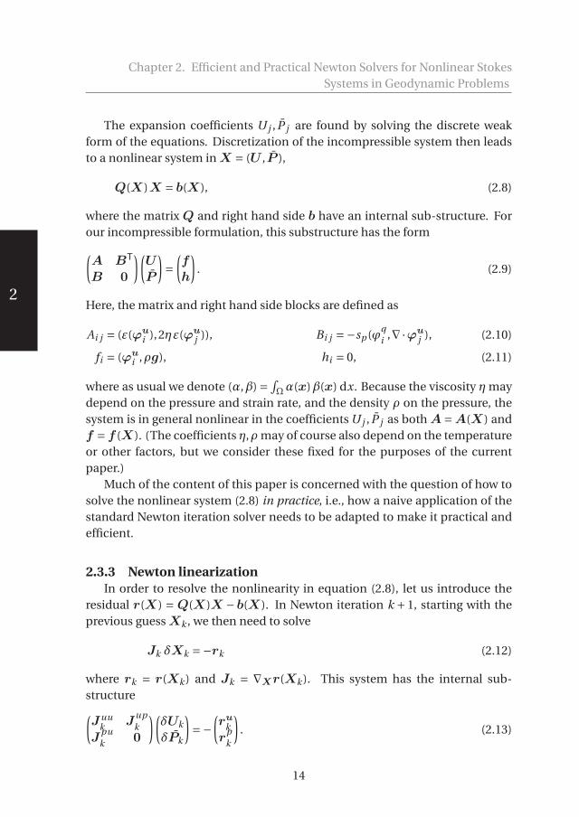
The expansion coefficients U j , P j are found by solving the discrete weakform of the equations. Discretization of the incompressible system then leadsto a nonlinear system in X = (U ,P ),
Q(X)X = b(X), (2.8)
where the matrix Q and right hand side b have an internal sub-structure. Forour incompressible formulation, this substructure has the form(A BT
B 0
)(UP
)=(fh
). (2.9)
Here, the matrix and right hand side blocks are defined as
Ai j = (ε(ϕui ),2ηε(ϕu
j )), Bi j =−sp (ϕqi ,∇·ϕu
j ), (2.10)
fi = (ϕui ,ρg), hi = 0, (2.11)
where as usual we denote (α,β) =∫Ωα(x)β(x) dx. Because the viscosity η maydepend on the pressure and strain rate, and the density ρ on the pressure, thesystem is in general nonlinear in the coefficients U j , P j as both A=A(X) andf = f (X). (The coefficients η,ρ may of course also depend on the temperatureor other factors, but we consider these fixed for the purposes of the currentpaper.)
Much of the content of this paper is concerned with the question of how tosolve the nonlinear system (2.8) in practice, i.e., how a naive application of thestandard Newton iteration solver needs to be adapted to make it practical andefficient.
2.3.3 Newton linearizationIn order to resolve the nonlinearity in equation (2.8), let us introduce the
residual r(X) = Q(X)X −b(X). In Newton iteration k + 1, starting with theprevious guess Xk , we then need to solve
Jk δXk =−rk (2.12)
where rk = r(Xk ) and Jk = ∇Xr(Xk ). This system has the internal sub-structure(Juu
k Jupk
Jpuk 0
)(δUk
δPk
)=−(rukr
pk
). (2.13)
14

530578-L-sub01-bw-Fraters530578-L-sub01-bw-Fraters530578-L-sub01-bw-Fraters530578-L-sub01-bw-FratersProcessed on: 10-4-2019Processed on: 10-4-2019Processed on: 10-4-2019Processed on: 10-4-2019 PDF page: 25PDF page: 25PDF page: 25PDF page: 25
2
2.3. Problem statement and numerical methods
After solving for δXk , we can compute Xk+1 = Xk +αk δXk where αk is astep length parameter that can be determined, for example, using a line search(Kelly, 1995; Nocedal and Wright, 1999).
There are a number of approaches to determining the entries of the matrixJk and to solving the resulting linear system. For example, in the geodynam-ics community alone, May et al. (2015) and Kaus et al. (2016) make use of aJacobian-free Newton-Krylov (JFNK) framework (see Knoll and Keyes (2004)),which essentially computes a finite difference approximation of J by evaluat-ing r at different values of its argument, and integrates this directly into thesolver so that the full Jacobian matrix is never built. On the other hand, Rudiet al. (2015) and Spiegelman et al. (2016) use the same approach as we will takehere and compute derivatives analytically or semi-analytically, except that Rudiet al. (2015) implemented this in a Jacobian-free manner.
Regardless of how exactly these derivatives are computed, the blocks of thelinear system for the Newton updates will have to have the following form(again omitting dependencies on quantities we consider frozen, such as thetemperature):(Juu
k
)i j =
∂
∂U j
(AkUk +BTPk −fk
)i
= (Ak )i j +(ε(ϕu
i ),2(∂η(ε(uk ), pk )
∂ε: ε(ϕu
j ))ε(uk )
), (2.14)
(J
upk
)i j= ∂
∂P j
(AkUk +BTPk −fk
)i
= BTi j +(ε(ϕu
i ),2(∂η(ε(uk ), pk )
∂pϕ
pj
)ε(uk )
),
= BTi j +(ε(ϕu
i ),2(∂η(ε(uk ), pk )
∂p
∂p
∂pϕ
pj
)ε(uk )
),
= BTi j + sp
(ε(ϕu
i ),2(∂η(ε(uk ), pk )
∂pϕ
pj
)ε(uk )
), (2.15)
(J
puk
)i j= ∂
∂U j(BUk −hk )i
= Bi j . (2.16)
It is easy to see that – as expected – the Newton system (2.13) reverts to the sim-ple Stokes problem if the viscosity does not depend on strain rate or pressure,i.e., if the system is linear.
As we will show below, while equation (2.12) (and its block structure (2.13))is the correct linearization of the (discretized) original, nonlinear system (2.3)
15
530578-L-sub01-bw-Fraters530578-L-sub01-bw-Fraters530578-L-sub01-bw-Fraters530578-L-sub01-bw-FratersProcessed on: 10-4-2019Processed on: 10-4-2019Processed on: 10-4-2019Processed on: 10-4-2019 PDF page: 26PDF page: 26PDF page: 26PDF page: 26
2
Chapter 2. Efficient and Practical Newton Solvers for Nonlinear StokesSystems in Geodynamic Problems
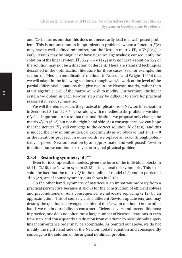
and (2.4), it turns out that this does not necessarily lead to a well-posed prob-lem. This is not uncommon in optimization problems where a function f (x)may have a well-defined minimizer, but the Hessian matrix Hk = ∇2 f (xk ) atearly iterates may be singular or have negative eigenvalues; consequently thesolution of the linear systemHk δxk =−∇ f (xk ) may not have a solution δxk orthe solution may not be a direction of descent. There are standard techniquesdescribed in the optimization literature for these cases (see, for example, thesection on “Hessian modification” methods in Nocedal and Wright (1999)) thatwe will adapt in the following sections, though we will work at the level of thepartial differential equations that give rise to the Newton matrix, rather thanat the algebraic level of the matrix we wish to modify. Furthermore, the linearsystem we obtain in each Newton step may be difficult to solve for practicalreasons if it is not symmetric.
We will therefore discuss the practical implications of Newton linearizationin Sections 2.3.4 and 2.3.5 below, along with remedies to the problems we iden-tify. It is important to stress that the modifications we propose only change thematrix Jk in (2.12) but not the right hand side. As a consequence, we can hopethat the iterates Xk still converge to the correct solution X of (2.8), and thisis indeed the case in our numerical experiments as we observe that ‖rk‖ → 0as the iterations proceed. In other words, we replace an exact (though poten-tially ill-posed) Newton iteration by an approximate (and well-posed) Newtoniteration, but we continue to solve the original physical problem.
2.3.4 Restoring symmetry of Juu
Even for incompressible models, given the form of the individual blocks in(2.14)–(2.16), the Newton system (2.13) is in general not symmetric. This is de-spite the fact that the matrix Q in the nonlinear model (2.8) and in particularA in (2.9) are of course symmetric, as shown in (2.10).
On the other hand, symmetry of matrices is an important property from apractical perspective because it allows for the construction of efficient solversand preconditioners. As a consequence, we advocate replacing (2.12) by anapproximation. This of course yields a different Newton update δxk and maydestroy the quadratic convergence order of the Newton method. On the otherhand, we retain our ability to construct efficient solvers and preconditioners;in practice, one does not often run a large number of Newton iterations in eachtime step, and consequently a reduction from quadratic to possibly only super-linear convergence order may be acceptable. As pointed out above, we do notmodify the right hand side of the Newton update equation and consequentlyconverge to the solution of the original nonlinear problem.
16

530578-L-sub01-bw-Fraters530578-L-sub01-bw-Fraters530578-L-sub01-bw-Fraters530578-L-sub01-bw-FratersProcessed on: 10-4-2019Processed on: 10-4-2019Processed on: 10-4-2019Processed on: 10-4-2019 PDF page: 27PDF page: 27PDF page: 27PDF page: 27
2
2.3. Problem statement and numerical methods
Specifically, then, we advocate for the following approximation of (2.14):
(Juu
k
)i j ≈ (Ak )i j +
(ε(ϕu
i ),(∂η(ε(uk ), pk )
∂ε: ε(ϕu
j ))ε(uk )
)+(ε(ϕu
j ),(∂η(ε(uk ), pk )
∂ε: ε(ϕu
i ))ε(uk )
).
This approximation ensures that the top left block in (2.13) is indeed symmet-ric, and as we will see below, this and the modification discussed in the nextsection will then allow for the construction of efficient, multigrid-based pre-conditioners and the use of the Conjugate Gradient method. Indeed, the mod-ification simply symmetrizes the second term in (2.14). In order to analyze theeffect of the underlying approximation, it is useful to rewrite the original termin (2.14) in sum notation:(ε(ϕu
i ),2(∂η(ε(uk ), pk )
∂ε: ε(ϕu
j ))ε(uk )
)=∫Ω
∑mn
ε(ϕui )mn
[∑pq
2∂η(ε(uk ), pk )
∂εpqε(ϕu
j )pq
]ε(uk )mn
=∫Ω
∑mn,pq
ε(ϕui )mnE(ε(uk ))mnpqε(ϕu
j )pq
where the rank-4 tensor E is defined as E(ε(u))mnpq =[
2ε(u)mn∂η(ε(u),p)
∂εpq
].
Clearly, the matrix Juuk is symmetric if the tensor E is symmetric, i.e., Emnpq =
Epqmn , but this is not always the case. (By its definition, we already haveEmnpq = Enmpq = Emnqp .) The modification we propose is equivalent to explic-itly symmetrizing this tensor, i.e., replacing Emnpq by E sym
mnpq = 12
(Emnpq +Epqmn
)and replacing the matrix in (2.14) by(Juu
k
)i j = (Ak )i j +
(ε(ϕu
i ),E sym(ε(uk )) ε(ϕuj ))
. (2.17)
It is instructive to consider whether there are cases in which the tensor E isalready symmetric, and replacing it by its symmetrized version consequentlydoes not change anything. Specifically, this is the case if the viscosity η(ε(u))can be written as a scalar function of the square of the strain rate, i.e., η(ε(u)) =f (‖ε(u)‖2) where ‖ε‖2 =∑i j ε
2i j . In this case, the chain rule implies that
∂η(ε(u))
∂εpq= f ′(‖ε(u)‖2)
∂‖ε(u)‖2
∂εpq= 2 f ′(‖ε(u)‖2) ε(u)pq .
17

530578-L-sub01-bw-Fraters530578-L-sub01-bw-Fraters530578-L-sub01-bw-Fraters530578-L-sub01-bw-FratersProcessed on: 10-4-2019Processed on: 10-4-2019Processed on: 10-4-2019Processed on: 10-4-2019 PDF page: 28PDF page: 28PDF page: 28PDF page: 28
2
Chapter 2. Efficient and Practical Newton Solvers for Nonlinear StokesSystems in Geodynamic Problems
We then have that E(ε(u))mnpq = 4 f ′(‖ε(u)‖2)ε(uk )mnε(u)pq , which satisfiesthe desired symmetry condition.
Furthermore, for incompressible materials, we have that trace ε(u) = divu=0, and in that case, the second invariant of the strain rate can be simplifiedto I2(ε(u)) = 1
2
[(trace ε(u))2 − trace (ε(u)2)
] = −12 trace (ε(u)2) = −1
2‖ε(u)‖2. Inother words, for incompressible materials, the second invariant is a function ofthe square of the norm of the strain rate, and consequently any material modelthat only depends on the second invariant then also satisfies the criteria forcases where the explicit symmetrization does not actually change anything. In-deed, many incompressible material models define the viscosity only in termsof the second invariant of the strain rate, see for example Schellart and Moresi(2013). (We note that the geodynamics literature uses varying definitions forthe second invariant. In contrast to the one used above, some papers use the
definition I2(ε(u)) = (12ε(u) : ε(u)
)1/2 = (12‖ε(u)‖2
)1/2– see, for example, Gerya
(2010, p. 56) or May et al. (2015). However, even with this convention the sec-ond invariant is a function of the square of the norm of the strain rate, and theconclusion above about material models that are functions of only the secondinvariant of the strain rate remains valid.)
We end by pointing out that the entire Jacobian remains non-symmetricsince, in general, Jup �= (Jpu)T because of the added term due to the deriva-tive of the viscosity with regard to the pressure (see (2.15) and (2.16)). We willcome back to this in Section 2.3.6.
2.3.5 Restoring well-posedness of the Newton step
The Stokes-like system (2.13) that arises from Newton linearization can onlybe well-posed if the top-left block is invertible. However, it turns out that thisis not always the case, as we will see shortly. It is important to realize, how-ever, that a lack of well-posedness of the Newton step is not equivalent to alack of well-posedness of the original, nonlinear problem from which it arises.Indeed, it is easy to conceive of situations where a Newton method applied tofinding solutions of one-dimensional equations f (x) = 0 fails because one ofthe intermediate iterates xk happens to land at a location where f ′(xk ) = 0 andthe next iteration fails because there is no δxk so that f ′(xk )δxk = − f (xk ). Inmultiple dimensions, and in particular in the case of the infinite dimensionaloperator from which the top-left matrix block Juu is derived, the situation isclearly more complex, but not much more complicated to understand.
18

530578-L-sub01-bw-Fraters530578-L-sub01-bw-Fraters530578-L-sub01-bw-Fraters530578-L-sub01-bw-FratersProcessed on: 10-4-2019Processed on: 10-4-2019Processed on: 10-4-2019Processed on: 10-4-2019 PDF page: 29PDF page: 29PDF page: 29PDF page: 29
2
2.3. Problem statement and numerical methods
To this end, recall that after the symmetrization discussed in the previoussection, the matrix Juu has entries
(Juu)i j =(ε(ϕu
i ),2η(ε(u))ε(ϕuj ))+(ε(ϕu
i ),E sym(ε(u))ε(ϕuj ))
= (ε(ϕui ),[2η(ε(u))I ⊗I +E sym(ε(u))
]︸ ︷︷ ︸=:H
ε(ϕuj )),
where the rank-4 tensor (I ⊗ I)i j kl = δi kδ j l maps a symmetric rank-2 tensoronto itself. A sufficient (though not necessary) condition for the matrix Juu tobe invertible (i.e., to have no zero eigenvalues) is if the corresponding differen-tial operator, −∇· [Hε(•)] is elliptic. This is the case if and only if the tensor H(as a map from rank-2 symmetric tensors to rank-2 symmetric tensors) has onlypositive eigenvalues, i.e., if ε : (Hε) > 0 for all symmetric, non-zero rank-2 ten-sors ε. (We provide a bit more mathematical background for this connectionbetween the coefficient H and the ellipticity of the corresponding differentialequation in Appendix 2.7.)
Informally, for a strain hardening material model, ∂η(ε(u))∂ε is positive, and
then so is 2η(ε(u))I⊗I+E sym(ε(u)) because E sym is a positive correction to thealready positive definite tensor 2ηI ⊗I . In other words, H would then be pos-itive as would the differential operator, and Juu would be an invertible matrix.The same would be true if the material model is strain weakening and if theamount of weakening is “small enough” because then the “small correction”E sym does not offset the positive definiteness of 2ηI⊗I . That said, we will needto be more formal with arguments as we are dealing with tensors instead ofscalars; the remainder of the section is therefore devoted to formalizing thesearguments and providing a solution to the problem.
Specifically, given the definitions above, the tensor H can be written as
H = 2η(ε(u))I ⊗I +E sym(ε(u))
= 2η(ε(u))I ⊗I +ε(u)⊗ ∂η(ε(u), p)
∂ε+ ∂η(ε(u), p)
∂ε⊗ε(u),
i.e., H is a rank-2 update of a multiple of the identity operator. The first of thesethree terms has all eigenvalues equal to 2η, and the other two terms then leadto a perturbation of two of these eigenvalues corresponding to eigendirections
that are spanned by ε(u) and ∂η(ε(u),p)∂ε . As mentioned above, unless a material’s
strain weakening rate is sufficiently small, these perturbations may be strongenough to make one or both of the perturbed eigenvalues negative, and in thiscase the Newton-step fails to be well-posed.
19

530578-L-sub01-bw-Fraters530578-L-sub01-bw-Fraters530578-L-sub01-bw-Fraters530578-L-sub01-bw-FratersProcessed on: 10-4-2019Processed on: 10-4-2019Processed on: 10-4-2019Processed on: 10-4-2019 PDF page: 30PDF page: 30PDF page: 30PDF page: 30
2
Chapter 2. Efficient and Practical Newton Solvers for Nonlinear StokesSystems in Geodynamic Problems
To avoid this, we introduce a tensor
H spd = 2η(ε(u))I ⊗I +αE sym(ε(u))
= 2η(ε(u))I ⊗I +α
[ε(u)⊗ ∂η(ε(u), p)
∂ε+ ∂η(ε(u), p)
∂ε⊗ε(u)
],
where 0 < α ≤ 1 is chosen in such a way that H spd is positive definite. Usingthis modified form of H spd at every quadrature point at which we perform theintegration of the bilinear form for the Newton matrix, we then build the matrixJuu used in the iteration. As before, since we do not change the right handside of the Newton update equation, we converge to the solution of the originalnonlinear problem.
Clearly, if α= 0, then H sym is the identity operator times 2η and has positiveeigenvalues. Because the eigenvalues depend continuously on α, there mustbe an α > 0 so that H spd is indeed positive definite. Ideally, to retain the con-vergence rate of Newton’s method, we would like to choose α= 1. We thereforepropose the following choice: we want to choose α so that (i) we have α= 1 if His already positive definite, (ii) α is as large as possible so that H spd is positivedefinite. In practice, however, we will also choose α small enough to avoid thecase where one of the eigenvalues of H spd is positive but very small comparedto 2η, to avoid the numerical difficulties resulting from trying to solve a linearproblem with a poorly conditioned matrix Juu .
It turns out that we can use the rank-2 update form of H and H spd to ex-plicitly compute the value of α. Let us abbreviate E sym = a ⊗b +b ⊗ a where
a = ε(u) and b = ∂η(ε(u),p)∂ε . Then it is clear that the (non-trivial) eigenvec-
tors of E sym must lie in the plane spanned by a,b, i.e., have the form v =cos(θ) a
‖a‖ + sin(θ) b‖b‖ . The two non-trivial eigenvalues of E sym are then the ex-
20

530578-L-sub01-bw-Fraters530578-L-sub01-bw-Fraters530578-L-sub01-bw-Fraters530578-L-sub01-bw-FratersProcessed on: 10-4-2019Processed on: 10-4-2019Processed on: 10-4-2019Processed on: 10-4-2019 PDF page: 31PDF page: 31PDF page: 31PDF page: 31
2
2.3. Problem statement and numerical methods
tremal values of the Rayleigh quotient
R(α) = v : (E sym : v)
=[
cos(θ)a
‖a‖ + sin(θ)b
‖b‖]
:
([a ⊗b +b ⊗a] :
[cos(θ)
a
‖a‖ + sin(θ)b
‖b‖])
= 2
[cos(θ)‖a‖+ sin(θ)
b : a
‖b‖][
cos(θ)b : a
‖a‖ + sin(θ)‖b‖]
= 2
[(b : a)cos(θ)2 +
((b : a)2
‖b‖‖a‖ +‖a‖‖b‖)
sin(θ)cos(θ)+ (b : a)sin(θ)2]
= 2
[(b : a)+
((b : a)2
‖b‖‖a‖ +‖a‖‖b‖)
sin(θ)cos(θ)
]= 2
[(b : a)+ 1
2
((b : a)2
‖b‖‖a‖ +‖a‖‖b‖)
sin(2θ)
]= 2
[b : a
‖a‖‖b‖ + 1
2
((b : a)2
‖b‖2‖a‖2 +1
)sin(2θ)
]‖a‖‖b‖.
Thus, the eigenvalues of E sym are given by[
2 b:a‖a‖‖b‖ ±
((b:a)2
‖b‖2‖a‖2 +1)]‖a‖‖b‖. In
other words, there is one positive eigenvalue λmax(E sym) =[
1+ b:a‖a‖‖b‖
]2 ‖a‖‖b‖and one negative or zero eigenvalue λmin(E sym) =−
[1− b:a
‖a‖‖b‖]2 ‖a‖‖b‖.
The only eigenvalue of H spd we have to worry about becoming negative istherefore the one associated with the (possibly) negative eigenvalue of E sym,
i.e., 2η(ε(u)) − α[
1− b:a‖a‖‖b‖
]2 ‖a‖‖b‖. This implies that we can choose the
damping factor α as follows to ensure positive semi-definiteness:
α=
⎧⎪⎨⎪⎩1 if
[1− b:a
‖a‖‖b‖]2 ‖a‖‖b‖ < 2η(ε(u))
2η(ε(u))[1− b:a
‖a‖‖b‖]2‖a‖‖b‖
otherwise.
In practice, we would like to stay well away from a zero eigenvalue and in-stead choose α as follows:
α=
⎧⎪⎨⎪⎩1 if
[1− b:a
‖a‖‖b‖]2 ‖a‖‖b‖ < csafety 2η(ε(u))
csafety2η(ε(u))[
1− b:a‖a‖‖b‖
]2‖a‖‖b‖otherwise,
(2.18)
where 0 ≤ csafety < 1 is a safety factor that ensures that the smaller eigenvalueof H spd is at least (1− csafety)2η and thus bounded away from zero. This com-putation is easily performed at every quadrature point during the assembly of
21

530578-L-sub01-bw-Fraters530578-L-sub01-bw-Fraters530578-L-sub01-bw-Fraters530578-L-sub01-bw-FratersProcessed on: 10-4-2019Processed on: 10-4-2019Processed on: 10-4-2019Processed on: 10-4-2019 PDF page: 32PDF page: 32PDF page: 32PDF page: 32
2
Chapter 2. Efficient and Practical Newton Solvers for Nonlinear StokesSystems in Geodynamic Problems
Juu . This procedure then guarantees that the resulting matrix is symmetricand positive definite, implying that the Newton direction is well defined.
It is again instructive to consider whether there are cases where we canalways choose α = 1, i.e., use the unmodified Newton step (possibly up tothe symmetrization discussed in the previous section). The simplest case is ifa : b = ‖a‖‖b‖ because in that case the definition of α in (2.18) always ends upin the first branch, regardless of the size of η(ε(u)). Given the definition of a,b,
this is specifically the case if ∂η(ε(u),p)∂ε is a positive multiple of ε(u). Similarly
to the discussion in the previous section, this is the case if η(ε(u)) = f (‖ε(u)‖2)and if f ′ ≥ 0, i.e., for a strain-hardening material. It is not difficult to show thatthis extends to the case where the viscosity is given by a non-decreasing func-tion η(ε(u)) = f (‖Pε(u)‖2) where P is an orthogonal projection applied to thestrain rate; an example is the operator that extracts the deviatoric componentof the strain rate.
A more interesting case is where the material exhibits strain weakening. Inthat case, intuitively the conditions in (2.18) imply that we can only choose α=1 if the material “weakens slowly enough”. Let us, for example, consider theclass of materials for which η(ε(u)) = η0 [I2(ε(u))]
1n −1. Such laws are typically
used to describe either diffusion (n = 1) or dislocation creep (n > 1), see Karato(2012). Indeed, we show in Appendix 2.8 that in these cases one has to alwayschoose α< 1 if n exceeds a certain threshold.
2.3.6 Algorithms for the solution of the nonlinear problemThe discussions of the previous sections show that a naive application of
Newton’s method may lead to matrices that are neither symmetric nor positivedefinite. Indeed, in some cases the equations for the Newton update may notbe well-posed at all (see, for example, the discussion in Appendix 2.8), even ifthe original, nonlinear model has all of these properties.
The remedies outlined above restore symmetry, positive definiteness, andwell-posedness, and consequently lend themselves for a practical implemen-tation. On the other hand, the resulting equations for the update are differ-ent from the ones obtained by linearizing the residual, and consequently wemay not be able to expect quadratic convergence of the resulting nonlinear it-eration. Indeed, this is what we will observe in the experiments we show inSection 2.4. Regardless, the modifications have to be incorporated into an ac-tual algorithm to solve the nonlinear problem. The algorithm we propose forthis – which is also the one implemented in the ASPECT code (Kronbichleret al., 2012; Heister et al., 2017) – is therefore outlined below. As for many other
22
530578-L-sub01-bw-Fraters530578-L-sub01-bw-Fraters530578-L-sub01-bw-Fraters530578-L-sub01-bw-FratersProcessed on: 10-4-2019Processed on: 10-4-2019Processed on: 10-4-2019Processed on: 10-4-2019 PDF page: 33PDF page: 33PDF page: 33PDF page: 33
2
2.3. Problem statement and numerical methods
nonlinear problems, it is not easy to universally achieve convergence, and theresulting algorithm is therefore complicated.
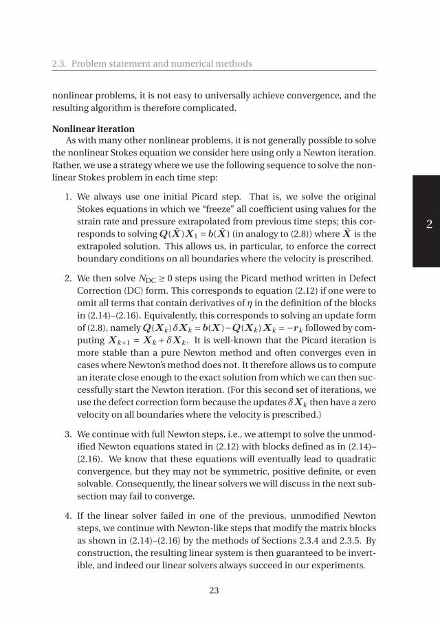
Nonlinear iterationAs with many other nonlinear problems, it is not generally possible to solve
the nonlinear Stokes equation we consider here using only a Newton iteration.Rather, we use a strategy where we use the following sequence to solve the non-linear Stokes problem in each time step:
1. We always use one initial Picard step. That is, we solve the originalStokes equations in which we “freeze” all coefficient using values for thestrain rate and pressure extrapolated from previous time steps; this cor-responds to solving Q(X)X1 = b(X) (in analogy to (2.8)) where X is theextrapoled solution. This allows us, in particular, to enforce the correctboundary conditions on all boundaries where the velocity is prescribed.
2. We then solve NDC ≥ 0 steps using the Picard method written in DefectCorrection (DC) form. This corresponds to equation (2.12) if one were toomit all terms that contain derivatives of η in the definition of the blocksin (2.14)–(2.16). Equivalently, this corresponds to solving an update formof (2.8), namely Q(Xk )δXk = b(X)−Q(Xk )Xk =−rk followed by com-puting Xk+1 = Xk +δXk . It is well-known that the Picard iteration ismore stable than a pure Newton method and often converges even incases where Newton’s method does not. It therefore allows us to computean iterate close enough to the exact solution from which we can then suc-cessfully start the Newton iteration. (For this second set of iterations, weuse the defect correction form because the updates δXk then have a zerovelocity on all boundaries where the velocity is prescribed.)
3. We continue with full Newton steps, i.e., we attempt to solve the unmod-ified Newton equations stated in (2.12) with blocks defined as in (2.14)–(2.16). We know that these equations will eventually lead to quadraticconvergence, but they may not be symmetric, positive definite, or evensolvable. Consequently, the linear solvers we will discuss in the next sub-section may fail to converge.
4. If the linear solver failed in one of the previous, unmodified Newtonsteps, we continue with Newton-like steps that modify the matrix blocksas shown in (2.14)–(2.16) by the methods of Sections 2.3.4 and 2.3.5. Byconstruction, the resulting linear system is then guaranteed to be invert-ible, and indeed our linear solvers always succeed in our experiments.
23
530578-L-sub01-bw-Fraters530578-L-sub01-bw-Fraters530578-L-sub01-bw-Fraters530578-L-sub01-bw-FratersProcessed on: 10-4-2019Processed on: 10-4-2019Processed on: 10-4-2019Processed on: 10-4-2019 PDF page: 34PDF page: 34PDF page: 34PDF page: 34
2
Chapter 2. Efficient and Practical Newton Solvers for Nonlinear StokesSystems in Geodynamic Problems
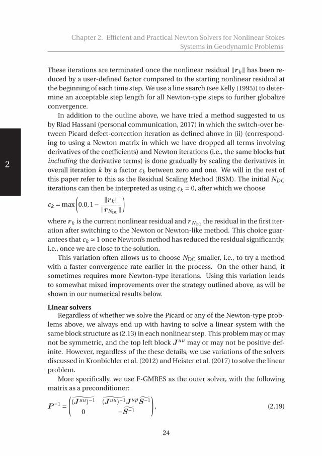
These iterations are terminated once the nonlinear residual ‖rk‖ has been re-duced by a user-defined factor compared to the starting nonlinear residual atthe beginning of each time step. We use a line search (see Kelly (1995)) to deter-mine an acceptable step length for all Newton-type steps to further globalizeconvergence.
In addition to the outline above, we have tried a method suggested to usby Riad Hassani (personal communication, 2017) in which the switch-over be-tween Picard defect-correction iteration as defined above in (ii) (correspond-ing to using a Newton matrix in which we have dropped all terms involvingderivatives of the coefficients) and Newton iterations (i.e., the same blocks butincluding the derivative terms) is done gradually by scaling the derivatives inoverall iteration k by a factor ck between zero and one. We will in the rest ofthis paper refer to this as the Residual Scaling Method (RSM). The initial NDC
iterations can then be interpreted as using ck = 0, after which we choose
ck = max
(0.0,1− ‖rk‖
‖rNDC‖)
where rk is the current nonlinear residual and rNDC the residual in the first iter-ation after switching to the Newton or Newton-like method. This choice guar-antees that ck ≈ 1 once Newton’s method has reduced the residual significantly,i.e., once we are close to the solution.
This variation often allows us to choose NDC smaller, i.e., to try a methodwith a faster convergence rate earlier in the process. On the other hand, itsometimes requires more Newton-type iterations. Using this variation leadsto somewhat mixed improvements over the strategy outlined above, as will beshown in our numerical results below.
Linear solversRegardless of whether we solve the Picard or any of the Newton-type prob-
lems above, we always end up with having to solve a linear system with thesame block structure as (2.13) in each nonlinear step. This problem may or maynot be symmetric, and the top left block Juu may or may not be positive def-inite. However, regardless of the these details, we use variations of the solversdiscussed in Kronbichler et al. (2012) and Heister et al. (2017) to solve the linearproblem.
More specifically, we use F-GMRES as the outer solver, with the followingmatrix as a preconditioner:
P −1 =(�(Juu)−1 �(Juu)−1JupS−1
0 −S−1
), (2.19)
24
530578-L-sub01-bw-Fraters530578-L-sub01-bw-Fraters530578-L-sub01-bw-Fraters530578-L-sub01-bw-FratersProcessed on: 10-4-2019Processed on: 10-4-2019Processed on: 10-4-2019Processed on: 10-4-2019 PDF page: 35PDF page: 35PDF page: 35PDF page: 35
2
2.3. Problem statement and numerical methods
where a tilde indicates an approximation of the matrix under the tilde, and S =Jpu(Juu)−1Jup is the Schur complement of the system. Specifically, motivatedby the discussions in Kronbichler et al. (2012) and Heister et al. (2017), we usethe following approximations for each of these blocks:
• �(Juu)−1: We approximate this matrix using either one multigrid cycle or afull solve with an approximation Juu of Juu that is constructed in a sim-ilar way as discussed in Kronbichler et al. (2012). In addition, becauseboth multigrid and the Conjugate Gradient method used here requireJuu to be symmetric and positive definite, we always apply the modi-fications of Sections 2.3.4 and 2.3.5, even if they are not applied to Juu
itself.
• S−1: This block is an approximation to the inverse of the Schur com-plement S = Jpu(Juu)−1Jup . Like for the original Stokes problem,the appropriate approximation is to use S−1 = M−1
p where (Mp )i j =(ϕ
pi , 1
η(ε(u))ϕpj ))
is the mass matrix on the pressure space scaled by the
inverse of the viscosity; the inversion of Mp is facilitated by a ConjugateGradient solve.
The approximation S−1 =M−1p is known to be good if Jpu = (Jup )T, see
Silvester and Wathen (1994). On the other hand, this is not the case if theviscosity depends on the pressure, given the additional term in (2.15).However, the difference between the two matrices is small if the viscositydoes not strongly depend on the pressure. This is, in fact, a commonlymade assumption, at least for deep Earth mantle models, though it maynot be valid for crustal models that employ pressure-dependent plasticitymodels.
It is conceivable that one can construct a better approximation S−1 forS−1 – leading to fewer outer F-GMRES iterations – by also incorporatingthe viscosity derivative terms somehow, but we did not pursue this direc-tion as it is tangential to the purpose of this paper.
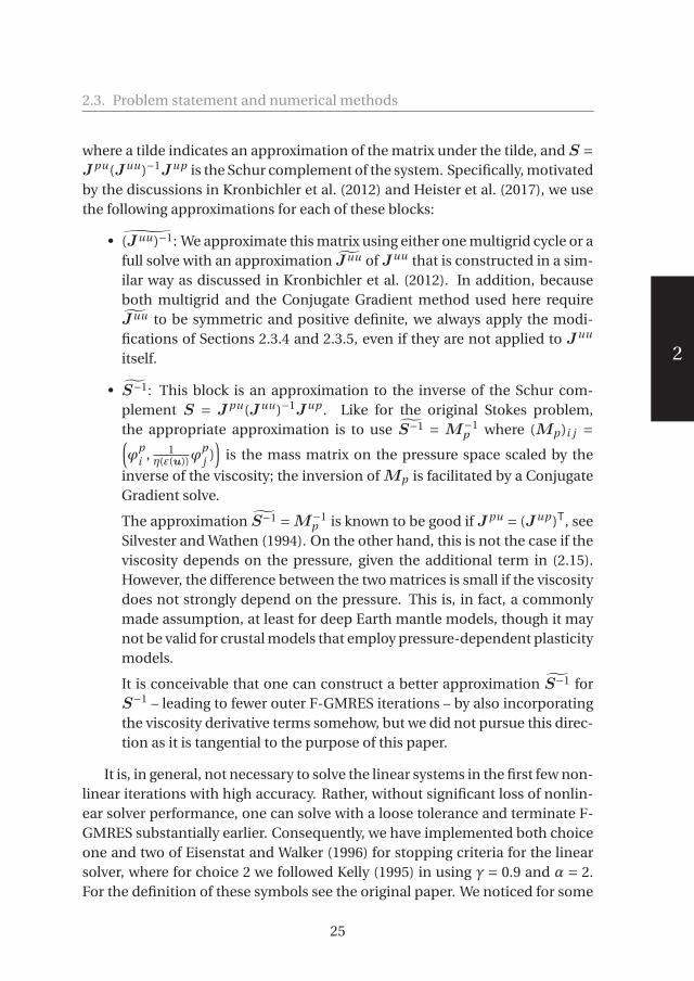
It is, in general, not necessary to solve the linear systems in the first few non-linear iterations with high accuracy. Rather, without significant loss of nonlin-ear solver performance, one can solve with a loose tolerance and terminate F-GMRES substantially earlier. Consequently, we have implemented both choiceone and two of Eisenstat and Walker (1996) for stopping criteria for the linearsolver, where for choice 2 we followed Kelly (1995) in using γ = 0.9 and α = 2.For the definition of these symbols see the original paper. We noticed for some
25

530578-L-sub01-bw-Fraters530578-L-sub01-bw-Fraters530578-L-sub01-bw-Fraters530578-L-sub01-bw-FratersProcessed on: 10-4-2019Processed on: 10-4-2019Processed on: 10-4-2019Processed on: 10-4-2019 PDF page: 36PDF page: 36PDF page: 36PDF page: 36
2
Chapter 2. Efficient and Practical Newton Solvers for Nonlinear StokesSystems in Geodynamic Problems
of the problems that the difference between these two approaches where sig-nificant, where the first choice allowed for a much loser tolerance. Eisenstatand Walker (1996) stated that choice one represents a direct relation betweenthe Newton right hand side F and its local linear model at the previous nonlin-ear iteration, while choice two is only an approximation of this. Therefore wehave chosen the first of these approaches for this paper.
Computation of derivativesImplementations of Newton solvers require concrete implementations of
the formulas for the derivatives ∂η(ε(u))∂ε and ∂η(ε(u))
∂p . These can be computed ei-ther using simple finite differencing approaches or analytically. Fortunately,even for relatively complicated material models, exact formulas for thesederivatives can be derived with modest effort. Examples for the material mod-els we consider in our numerical results below are provided in Appendix 2.8.
2.4 Numerical experiments using common benchmarksIn this section, let us illustrate the performance of the methods layed out
above, using several benchmarks that vary both in which specific elements ofthe solver they test as well as in the difficulty they present to solvers. In partic-ular, we will assess whether and how fast different variations of our algorithmsconverge. This includes ensuring that the nonlinear residual can be reduced toany small value desired. Furthermore, we will investigate optimal values andrelative trade-offs for a variety of parameters that affect the nonlinear solverscheme, as discussed in Section 2.3.6.
The benchmarks we describe here have all been used for similar purposesin the literature. Details of all of our experiments are, sometimes in a simplifiedform, also part of the ASPECT test suite. All codes necessary to run these ex-periments are available among the benchmarks included in ASPECT releasesstarting from version 2.1. The ASPECT repository can be found athttps://github.com/geodynamics/aspect.
2.4.1 Nonlinear channel flowThe simplest nonlinear Stokes flow one can think of is probably a gener-
alization of incompressible Poiseuille flow to include a strain-rate dependentviscosity. In it, one forces a fluid through a pipe or channel where the velocityis zero at the pipe sides and in- and outflow velocities are prescribed in sucha way that the result is a flow field parallel to the pipe axis and constant in thealong-pipe direction. The across-pipe variation of the velocity field can then
26
530578-L-sub01-bw-Fraters530578-L-sub01-bw-Fraters530578-L-sub01-bw-Fraters530578-L-sub01-bw-FratersProcessed on: 10-4-2019Processed on: 10-4-2019Processed on: 10-4-2019Processed on: 10-4-2019 PDF page: 37PDF page: 37PDF page: 37PDF page: 37
2
2.4. Numerical experiments using common benchmarks
be computed easily once a rheology law is chosen, leading to an analyticallyknown flow field from which the in- and outflow boundary conditions can alsobe drawn either via prescribed velocities or prescribed tractions.
A visualization of the solution can be found, for example, in Gerya (2010);Turcotte and Schubert (2002).
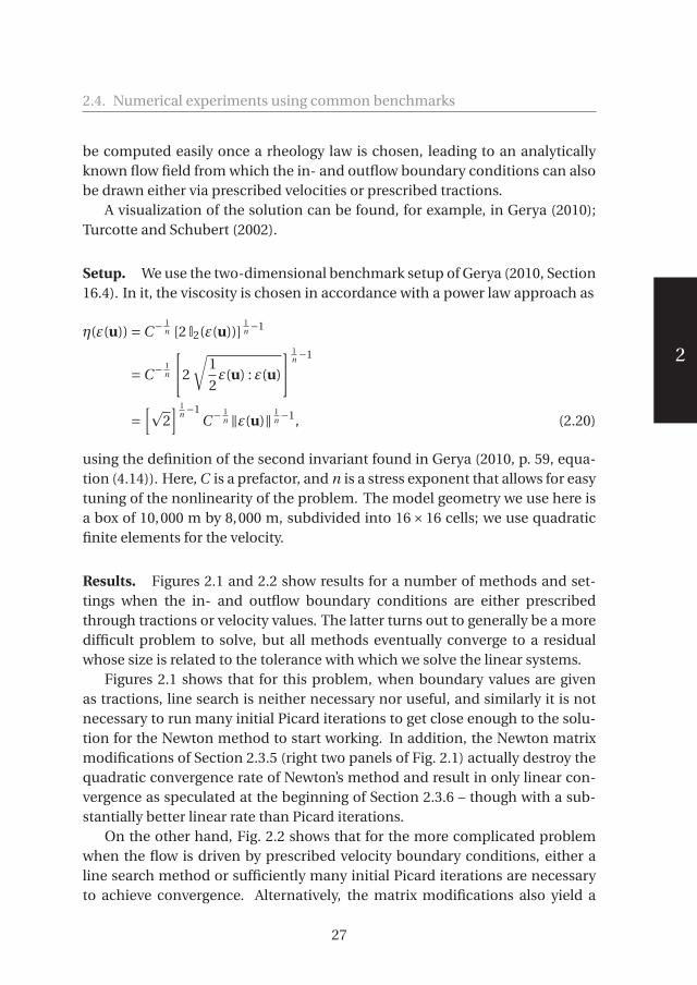
Setup. We use the two-dimensional benchmark setup of Gerya (2010, Section16.4). In it, the viscosity is chosen in accordance with a power law approach as
η(ε(u)) =C− 1n [2 I2(ε(u))]
1n −1
=C− 1n
[2
√1
2ε(u) : ε(u)
] 1n −1
=[�
2] 1
n −1C− 1
n ‖ε(u)‖ 1n −1, (2.20)
using the definition of the second invariant found in Gerya (2010, p. 59, equa-tion (4.14)). Here, C is a prefactor, and n is a stress exponent that allows for easytuning of the nonlinearity of the problem. The model geometry we use here isa box of 10,000 m by 8,000 m, subdivided into 16×16 cells; we use quadraticfinite elements for the velocity.
Results. Figures 2.1 and 2.2 show results for a number of methods and set-tings when the in- and outflow boundary conditions are either prescribedthrough tractions or velocity values. The latter turns out to generally be a moredifficult problem to solve, but all methods eventually converge to a residualwhose size is related to the tolerance with which we solve the linear systems.
Figures 2.1 shows that for this problem, when boundary values are givenas tractions, line search is neither necessary nor useful, and similarly it is notnecessary to run many initial Picard iterations to get close enough to the solu-tion for the Newton method to start working. In addition, the Newton matrixmodifications of Section 2.3.5 (right two panels of Fig. 2.1) actually destroy thequadratic convergence rate of Newton’s method and result in only linear con-vergence as speculated at the beginning of Section 2.3.6 – though with a sub-stantially better linear rate than Picard iterations.
On the other hand, Fig. 2.2 shows that for the more complicated problemwhen the flow is driven by prescribed velocity boundary conditions, either aline search method or sufficiently many initial Picard iterations are necessaryto achieve convergence. Alternatively, the matrix modifications also yield a
27
530578-L-sub01-bw-Fraters530578-L-sub01-bw-Fraters530578-L-sub01-bw-Fraters530578-L-sub01-bw-FratersProcessed on: 10-4-2019Processed on: 10-4-2019Processed on: 10-4-2019Processed on: 10-4-2019 PDF page: 38PDF page: 38PDF page: 38PDF page: 38
2
Chapter 2. Efficient and Practical Newton Solvers for Nonlinear StokesSystems in Geodynamic Problems
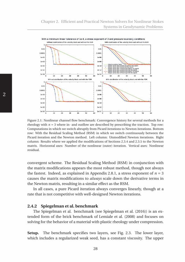
Figure 2.1: Nonlinear channel flow benchmark: Convergence history for several methods for arheology with n = 3 where in- and outflow are described by prescribing the traction. Top row:Computations in which we switch abruptly from Picard iterations to Newton iterations. Bottomrow: With the Residual Scaling Method (RSM) in which we switch continuously between thePicard iteration and the Newton method. Left column: Unmodified Newton iterations. Rightcolumn: Results where we applied the modifications of Sections 2.3.4 and 2.3.5 to the Newtonmatrix. Horizontal axes: Number of the nonlinear (outer) iteration. Vertical axes: Nonlinearresidual.
convergent scheme. The Residual Scaling Method (RSM) in conjunction withthe matrix modifications appears the most robust method, though not alwaysthe fastest. Indeed, as explained in Appendix 2.8.1, a stress exponent of n = 3causes the matrix modifications to always scale down the derivative terms inthe Newton matrix, resulting in a similar effect as the RSM.
In all cases, a pure Picard iteration always converges linearly, though at arate that is not competitive with well-designed Newton iterations.
2.4.2 Spiegelman et al. benchmarkThe Spiegelman et al. benchmark (see Spiegelman et al. (2016)) is an ex-
tended form of the brick benchmark of Lemiale et al. (2008) and focuses onsolving for the behavior of a material with plastic rheology under compression.
Setup. The benchmark specifies two layers, see Fig. 2.3. The lower layer,which includes a regularized weak seed, has a constant viscosity. The upper
28

530578-L-sub01-bw-Fraters530578-L-sub01-bw-Fraters530578-L-sub01-bw-Fraters530578-L-sub01-bw-FratersProcessed on: 10-4-2019Processed on: 10-4-2019Processed on: 10-4-2019Processed on: 10-4-2019 PDF page: 39PDF page: 39PDF page: 39PDF page: 39
2
2.4. Numerical experiments using common benchmarks
Figure 2.2: Nonlinear channel flow benchmark: Convergence history for several methods for arheology with n = 3 where in- and outflow are described by prescribing the velocity. Panels as inFig. 2.1.
layer has a viscosity given by the harmonic mean ηeff = η1ηp
η1+ηp. Here, η1 is the
background viscosity of the upper layer, and
ηp = A+B(plith +αp ′)2 I2(ε(u))
,
where plith is the depth dependent lithostatic pressure and p ′ = p −plith is thedynamic component of the total pressure. η1 can have three different val-ues: 1e23, 1e24 and 5e24 Pa s. For von Mises plasticity, one would chooseA =C ,B = 0 where C is the cohesion of the material; in this case, the viscosity isstrain-rate but not pressure dependent. For a depth-dependent von Mises-typemodel, one would choose A = C cos(φ),B = sin(φ),α = 0 where φ is the fric-tion angle; in this case, the viscosity depends on the static, lithospheric pres-sure but not the dynamic pressure component. Finally, Drucker-Prager plas-ticity fits this formula with A = C cos(φ),B = sin(φ),α = 1 where the viscositynow depends on both the strain rate and the (total) pressure p = plith +p ′. Wewill only consider the von Mises and Drucker-Prager cases of the Spiegelmanbenchmark because these are the most interesting ones.
The benchmark is completed by prescribing an inbound velocity (2.5, 5 and12.5 mm/yr) on the two sides of the geometry, requiring tangential flow at the
29

530578-L-sub01-bw-Fraters530578-L-sub01-bw-Fraters530578-L-sub01-bw-Fraters530578-L-sub01-bw-FratersProcessed on: 10-4-2019Processed on: 10-4-2019Processed on: 10-4-2019Processed on: 10-4-2019 PDF page: 40PDF page: 40PDF page: 40PDF page: 40
2
Chapter 2. Efficient and Practical Newton Solvers for Nonlinear StokesSystems in Geodynamic Problems
Figure 2.3: Spiegelman et al. benchmark: Depiction of the strain rate and velocity field (top),viscosity (bottom left) and the SPD factor α (bottom right) as a result of the deformation inducedby the prescribed horizontal velocity on the sides of the domain. The results shown here are forthe case where the velocities are 5mm/year (the color bar shows it in m/s, ηref = 1024 Pas, theangle of internal friction is 30◦ and the mesh consists of 1024×256 cells. This is one of the moredifficult cases (Drucker-Prager) of the benchmark, and the data shown here are the result ofsimulations that are only converged to a relative nonlinear residual of about 10−6.
bottom, and no stress at the top, allowing material to leave the domain. Thethree options for the inbound velocity and the three options for the referencebackground viscosity together form a set of nine test cases whose difficulty in-creases with velocity and reference background viscosity. In the original pa-per, an unstructured grid of stable Taylor-Hood elements was used. Based ontheir Fig. 1, the results shown there should, based on the length of the edges,correspond to a uniform ASPECT mesh that has been refined globally approx-imately 7 or 8 times (i.e., 512×128 or 1024×256 cells). This does not, however,account for details of the unstructured mesh used in Spiegelman et al. (2016).
Results. We compare the results of our Newton implementation to the resultsof Spiegelman et al. (2016) and the pre-existing Picard solver in ASPECT. Thevon Mises case results are quite similar to the results from Spiegelman et al.(2016); consequently, we will focus on the more difficult Drucker-Prager case.We have exhaustively explored the space of parameters affecting the nonlinearsolver (see Section 2.3.6) at different mesh resolutions. In general, we found
30

530578-L-sub01-bw-Fraters530578-L-sub01-bw-Fraters530578-L-sub01-bw-Fraters530578-L-sub01-bw-FratersProcessed on: 10-4-2019Processed on: 10-4-2019Processed on: 10-4-2019Processed on: 10-4-2019 PDF page: 41PDF page: 41PDF page: 41PDF page: 41
2
2.4. Numerical experiments using common benchmarks
Figure 2.4: Spiegelman et al. benchmark: A reproduction of three of the nine pressure dependentDrucker-Prager cases with a resolution of 64×16 cells (substantially coarser than the resolutionin the Spiegelman et al. (2016)). Top: Results for computations where linear systems are solvedwith a relative tolerance of 0.9. Bottom: With a tolerance of 10−8. The initial Picard iteration isalways solved to a linear tolerance of 10−16. Left to right: Different prescribed velocities of u0 =2.5, 5, and 12.5cm/year and different reference viscsocities of respectively ηref = 1023, 1024 and5×1024 Pa s . Horizontal axis: Number of the nonlinear (outer) iteration; vertical axis: Nonlinearresidual. DC Picard refers to a Defect Correction Picard iteration, see Section 2.3.6.
that higher mesh resolution (more refinement steps) made the problem moredifficult to solve. As expected, the benchmarks also become more difficult asthe prescribed velocity u0 at the boundary is increased, leading to a larger strainrate and more pronounced nonlinearity. This is visible in Fig. 2.3 where we alsoshow the viscosity and the α factor necessary to keep the matrix positive def-inite. This factor drops to approximately one half in the vicinity of the shearband – a result consistent with the theoretical considerations discussed in Ap-pendix 2.8.3.
Figures 2.4 and 2.5 show results obtained for 4 and 8 global mesh refine-ment steps, corresponding to meshes with 64×16 and 1024×256 cells, respec-tively. A comparison shows that the problem is indeed more difficult to solveon the finer meshes. Without enforcing the symmetry and positive definitenessof the top left block of the Jacobian, the linear solver converges quickly, but alsocrashes easily in a number of configurations because the matrix lacks the nec-essary structural properties; this is particularly the case for u0 = 12.5 mm/year.
31
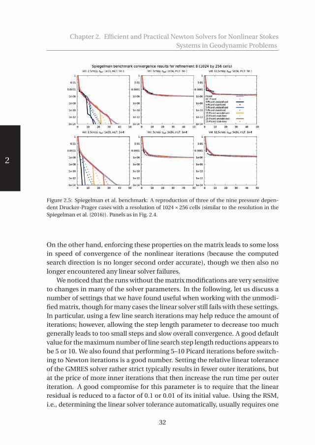
530578-L-sub01-bw-Fraters530578-L-sub01-bw-Fraters530578-L-sub01-bw-Fraters530578-L-sub01-bw-FratersProcessed on: 10-4-2019Processed on: 10-4-2019Processed on: 10-4-2019Processed on: 10-4-2019 PDF page: 42PDF page: 42PDF page: 42PDF page: 42
2
Chapter 2. Efficient and Practical Newton Solvers for Nonlinear StokesSystems in Geodynamic Problems
Figure 2.5: Spiegelman et al. benchmark: A reproduction of three of the nine pressure depen-dent Drucker-Prager cases with a resolution of 1024×256 cells (similar to the resolution in theSpiegelman et al. (2016)). Panels as in Fig. 2.4.
On the other hand, enforcing these properties on the matrix leads to some lossin speed of convergence of the nonlinear iterations (because the computedsearch direction is no longer second order accurate), though we then also nolonger encountered any linear solver failures.
We noticed that the runs without the matrix modifications are very sensitiveto changes in many of the solver parameters. In the following, let us discuss anumber of settings that we have found useful when working with the unmodi-fied matrix, though for many cases the linear solver still fails with these settings.In particular, using a few line search iterations may help reduce the amount ofiterations; however, allowing the step length parameter to decrease too muchgenerally leads to too small steps and slow overall convergence. A good defaultvalue for the maximum number of line search step length reductions appears tobe 5 or 10. We also found that performing 5–10 Picard iterations before switch-ing to Newton iterations is a good number. Setting the relative linear toleranceof the GMRES solver rather strict typically results in fewer outer iterations, butat the price of more inner iterations that then increase the run time per outeriteration. A good compromise for this parameter is to require that the linearresidual is reduced to a factor of 0.1 or 0.01 of its initial value. Using the RSM,i.e., determining the linear solver tolerance automatically, usually requires one
32
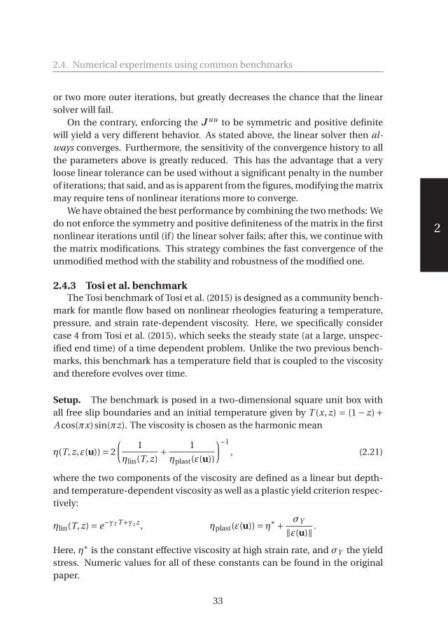
530578-L-sub01-bw-Fraters530578-L-sub01-bw-Fraters530578-L-sub01-bw-Fraters530578-L-sub01-bw-FratersProcessed on: 10-4-2019Processed on: 10-4-2019Processed on: 10-4-2019Processed on: 10-4-2019 PDF page: 43PDF page: 43PDF page: 43PDF page: 43
2
2.4. Numerical experiments using common benchmarks
or two more outer iterations, but greatly decreases the chance that the linearsolver will fail.
On the contrary, enforcing the Juu to be symmetric and positive definitewill yield a very different behavior. As stated above, the linear solver then al-ways converges. Furthermore, the sensitivity of the convergence history to allthe parameters above is greatly reduced. This has the advantage that a veryloose linear tolerance can be used without a significant penalty in the numberof iterations; that said, and as is apparent from the figures, modifying the matrixmay require tens of nonlinear iterations more to converge.
We have obtained the best performance by combining the two methods: Wedo not enforce the symmetry and positive definiteness of the matrix in the firstnonlinear iterations until (if) the linear solver fails; after this, we continue withthe matrix modifications. This strategy combines the fast convergence of theunmodified method with the stability and robustness of the modified one.
2.4.3 Tosi et al. benchmarkThe Tosi benchmark of Tosi et al. (2015) is designed as a community bench-
mark for mantle flow based on nonlinear rheologies featuring a temperature,pressure, and strain rate-dependent viscosity. Here, we specifically considercase 4 from Tosi et al. (2015), which seeks the steady state (at a large, unspec-ified end time) of a time dependent problem. Unlike the two previous bench-marks, this benchmark has a temperature field that is coupled to the viscosityand therefore evolves over time.
Setup. The benchmark is posed in a two-dimensional square unit box withall free slip boundaries and an initial temperature given by T (x, z) = (1− z)+A cos(πx)sin(πz). The viscosity is chosen as the harmonic mean
η(T, z,ε(u)) = 2
(1
ηlin(T, z)+ 1
ηplast(ε(u))
)−1
, (2.21)
where the two components of the viscosity are defined as a linear but depth-and temperature-dependent viscosity as well as a plastic yield criterion respec-tively:
ηlin(T, z) = e−γT T+γz z , ηplast(ε(u)) = η∗ + σY
‖ε(u)‖ .
Here, η∗ is the constant effective viscosity at high strain rate, and σY the yieldstress. Numeric values for all of these constants can be found in the originalpaper.
33

530578-L-sub01-bw-Fraters530578-L-sub01-bw-Fraters530578-L-sub01-bw-Fraters530578-L-sub01-bw-FratersProcessed on: 10-4-2019Processed on: 10-4-2019Processed on: 10-4-2019Processed on: 10-4-2019 PDF page: 44PDF page: 44PDF page: 44PDF page: 44
2
Chapter 2. Efficient and Practical Newton Solvers for Nonlinear StokesSystems in Geodynamic Problems
Results. The original paper does not contain convergence plots. Conse-quently, we can only compare between the methods available in our referenceimplementation. Specifically, these are: (i) A method whereby we solve the ad-vection equation, then the Stokes equation with frozen coefficients, and theniterate these two steps out until we have reached convergence for the currenttime step; we will refer to this scheme as “Picard” even though this stretches theterm (as, strictly speaking, a “Picard” iteration for the coupled system wouldsolve both the Stokes and advection problem linearized around the previoussolution; in our implementation, the Stokes system is linearized around thealready computed advection solution). In ASPECT, this scheme is called “it-erated advection and Stokes”. (ii) A method where we first solve the advectionequation and then do one Newton step on the nonlinear Stokes system; again,these two parts are iterated out in each time step. We will refer to this methodas “Newton”; in ASPECT, it is called “iterated advection and Newton Stokes”.
Figure . 2.6 shows results for this benchmark, where the horizontal axis indi-cates the number of the nonlinear iteration performed. Each spike correspondsto a time step starting at a large residual that is gradually decreased. A methodthat converges quickly shows a steeper decrease, requires fewer nonlinear iter-ations, and can consequently fit more time steps (spikes) into the same numberof nonlinear iterations. Because the computational effort is largely confined tobuilding and solving the linear systems, the horizontal axis also correspondsclosely to the elapsed wall time.
The different panels of the figure can be summarized as follows: (i) TheNewton method converges much faster than Picard iterations. For example,after the initial few time steps, the Newton method (with and without matrixstabilization) only requires two nonlinear iterations per time step, whereas thePicard iteration requires six. This also translates to a speed up in wall time ofaround the same factor. (ii) Matrix stabilization is not necessary for this bench-mark and in fact leads to a slight but not substantial degradation of perfor-mance. (iii) Convergence behavior can differ substantially between timesteps(both for Picard and Newton). (iv) For this experiment, the defect correctionform of the Picard iteration is slightly, but not substantially faster than the orig-inal Picard iteration.
2.4.4 A 3d subduction test caseIn order to verify that our implementation is not only applicable to aca-
demic benchmarks, but also to settings that occur in geodynamic modeling, letus consider a three-dimensional simulation of oceanic plate subduction. The
34

530578-L-sub01-bw-Fraters530578-L-sub01-bw-Fraters530578-L-sub01-bw-Fraters530578-L-sub01-bw-FratersProcessed on: 10-4-2019Processed on: 10-4-2019Processed on: 10-4-2019Processed on: 10-4-2019 PDF page: 45PDF page: 45PDF page: 45PDF page: 45
2
2.4. Numerical experiments using common benchmarks
Figure 2.6: Tosi et al. benchmark: Nonlinear Stokes residual (vertical axis) as a function of thenumber of the nonlinear solves. Each spike corresponds to one time step during which itera-tions start with a large residual that is gradually decreased until it reaches the desired nonlineartolerance of 10−5. No line search is used here. Top: The first 50 nonlinear iterations. Bottom:Nonlinear iteration 500–600. Left: Linear systems are solved to a relative Linear Tolerance (LT) of0.9. Right: With a linear tolerance of 0.01. In the top right panel, the results for the two Newtonvariations coincide.
model is inspired by the geodynamic setting of the Caribbean region, and sim-ulates a slab that subducts while the subducting plate has a motion oblique tothe trench which causes the slab to be dragged laterally through the mantle, amotion called slab dragging (Spakman et al., 2018).
Setup. We situate our test case in a Cartesian box with dimensions of 3000 kmin width and length and 1000 km in depth (see Fig. 2.7). The viscoplastic rheol-ogy includes dislocation creep, diffusion creep, and plasticity. The viscosity isthen given by
ηeff = max
(min
{(1
ηdiff+ 1
ηdisl
)−1
, ηplastic, ηmax
},ηmin
)(2.22)
35

530578-L-sub01-bw-Fraters530578-L-sub01-bw-Fraters530578-L-sub01-bw-Fraters530578-L-sub01-bw-FratersProcessed on: 10-4-2019Processed on: 10-4-2019Processed on: 10-4-2019Processed on: 10-4-2019 PDF page: 46PDF page: 46PDF page: 46PDF page: 46
2
Chapter 2. Efficient and Practical Newton Solvers for Nonlinear StokesSystems in Geodynamic Problems
Figure 2.7: A conceptual visualization of the 3d subduction test case setup. The red layer repre-sents the lithosphere, the yellow layer the upper mantle, and the green layer the lower mantle.The arrows indicate the lithospheric boundary velocity direction.
Figure 2.8: Right: The viscosity field of the 3d subduction test case after 3.55·106 years, just as thetip of the subducting slab starts to detach from the rest of the slab. In the left half, two isosurfacesshow where in the bottom half of the model the viscosity equals 3.25 ·1019 and 5.5 ·1019 Pas. Inthe right half, colors indicate the viscosity when restricted to areas where the viscosity is greaterthan 5 ·1019 Pas, i.e., to cold areas of the upper mantle, as well as the lower mantle.
36
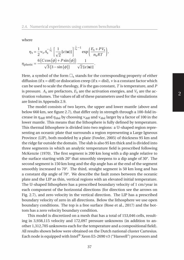
530578-L-sub01-bw-Fraters530578-L-sub01-bw-Fraters530578-L-sub01-bw-Fraters530578-L-sub01-bw-FratersProcessed on: 10-4-2019Processed on: 10-4-2019Processed on: 10-4-2019Processed on: 10-4-2019 PDF page: 47PDF page: 47PDF page: 47PDF page: 47
2
2.4. Numerical experiments using common benchmarks
where
ηx = 1
2νx A
− 1nx
x
[1�2‖ε(u)‖
] 1nx
−1
exp
(Ex +PVx
nxRT
),
ηplastic =6(C cos
(φ)+P sin
(φ))
�3(3− sin
(φ)) 1�
2‖ε(u)‖ .
Here, a symbol of the form �x stands for the corresponding property of eitherdiffusion (if x = diff) or dislocation creep (if x = disl), ν is a constant factor whichcan be used to scale the rheology, R is the gas constant, T is temperature, and Pis pressure. Ax are prefactors, Ex are the activation energies, and Vx are the ac-tivation volumes. The values of all of these parameters used for the simulationsare listed in Appendix 2.9.
The model consists of two layers, the upper and lower mantle (above andbelow 660 km, see figure 2.7), that differ only in strength through a 100-fold in-crease in ηdiff and ηdisl by choosing νdiff and νdisl larger by a factor of 100 in thelower mantle. This means that the lithosphere is fully defined by temperature.This thermal lithosphere is divided into two regions: a U-shaped region repre-senting an oceanic plate that surrounds a region representing a Large IgneousProvince (LIP), both modeled by a plate (Fowler, 2005) of thickness 95 km andthe ridge far outside the domain. The slab is also 95 km thick and is divided intothree segments in which an analytic temperature field is prescribed followingMcKenzie (1970). The first segment is 200 km long with a dip angle relative tothe surface starting with 20° that smoothly steepens to a dip angle of 30°. Thesecond segment is 150 km long and the dip angle has at the end of the segmentsmoothly increased to 70°. The third, straight segment is 50 km long and hasa constant dip angle of 70°. We describe the fault zones between the oceanicplate and the LIP as thin, vertical regions with an elevated initial temperature.The U-shaped lithosphere has a prescribed boundary velocity of 1 cm/year ineach component of the horizontal directions (for direction see the arrows onFig. 2.7), and zero velocity in the vertical direction. The LIP has a prescribedboundary velocity of zero in all directions. Below the lithosphere we use openboundary conditions. The top is a free surface (Rose et al., 2017) and the bot-tom has a zero velocity boundary condition.
This model is discretized on a mesh that has a total of 153,046 cells, result-ing in 3,938,115 velocity and 172,097 pressure unknowns (in addition to an-other 1,312,705 unknowns each for the temperature and a compositional field).All results shown below were obtained on the Dutch national cluster Cartesius.Each node is equipped with Intel® Xeon E5-2690 v3 (“Haswell”) processors and
37

530578-L-sub01-bw-Fraters530578-L-sub01-bw-Fraters530578-L-sub01-bw-Fraters530578-L-sub01-bw-FratersProcessed on: 10-4-2019Processed on: 10-4-2019Processed on: 10-4-2019Processed on: 10-4-2019 PDF page: 48PDF page: 48PDF page: 48PDF page: 48
2
Chapter 2. Efficient and Practical Newton Solvers for Nonlinear StokesSystems in Geodynamic Problems
Figure 2.9: The 3d subduction test case: Nonlinear convergence results for the Picard, DefectCorrection (DC) Picard, and Newton iterations. The horizontal axis shows time steps, with non-linear iterations depicted at 1
250 = 0.004 increments given that we allow at most 250 nonlineariterations per time step. The vertical axis represents the nonlinear relative residual.
has 24 cores; we used 10 nodes and 20 MPI processes per node. The modelis run with a Courant-Friedrichs-Lewy (CFL) number of 0.1 and the time stepsize is limited to grow by a maximum of 25% from one time step to the next.The time step sizes computed by all nonlinear solver methods used below areessentially identical.
The experiments in previous sections show that it is in general not neces-sary to solve the linear systems in defect correction schemes (i.e., the defectcorrect version of Picard iterations, as well as Newton iterations) particularlyaccurately. As a consequence, we only use a linear solver tolerance for thesemethods that requires a reduction of the linear residual in the F-GMRES solveby a factor of 0.1. On the other hand, the initial Picard iteration solves for thesolution, not an update, and consequently requires a substantially larger reduc-tion of the linear residual; we use a factor of 10−6 (the default value of ASPECT).
Results. We have performed this experiment using our implementation ofthe Newton method, as well as the Picard iteration and its defect correction(DC) variation. In the following, let us provide two perspectives on this com-parison.
First, Fig. 2.9 shows how all three methods reduce the nonlinear residualin each time step, for two selected periods of the simulation (from time steps75 to 100, and 275 to 300). In the early phases of the simulation, all methodsquickly converge the nonlinear residual to the desired tolerance of 10−6, thougheven here, the Newton method requires fewer iterations. Interestingly, startingaround time step 275 – corresponding to about 3.92 million years of model time
38

530578-L-sub01-bw-Fraters530578-L-sub01-bw-Fraters530578-L-sub01-bw-Fraters530578-L-sub01-bw-FratersProcessed on: 10-4-2019Processed on: 10-4-2019Processed on: 10-4-2019Processed on: 10-4-2019 PDF page: 49PDF page: 49PDF page: 49PDF page: 49
2
2.4. Numerical experiments using common benchmarks
Figure 2.10: The 3d subduction test case: Wall clock time necessary to compute up to a certaintime step for the Picard, Defect Correction (DC) Picard, and Newton iterations.
– the problem appears to become substantially more difficult to solve. Thistime corresponds to the break-off of the deeper part of the slab (the necking inFig. 2.8), which then rapidly sinks, and the increased velocity implies a largerstrain rate and consequently stronger nonlinearity. Indeed, as Fig. 2.9 shows,both variations of the Picard iteration are then no longer able to converge theresidual to the desired tolerance, even though we allow up to 250 iterations pertime step. Any results of these simulations must then necessarily be suspicious.On the other hand, the Newton iteration continues to rapidly converge. Thesedata therefore underline the stability and robustness of the Newton method,and illustrate that it can solve problems that are otherwise not solvable withreasonable effort.
A second perspective is shown in Fig. 2.10, where we plot the wall time nec-essary to solve the problem up to a given time step. The figure demonstratesthat our implementation of Newton’s method is approximately one third fasterthan the other two methods for the time steps shown. The difference becomesparticular notable after time step 170, where the subducting slab starts to thinunder its own gravity. We did not include data beyond time step 275 because,as discussed above, the Picard variants do not converge any more after thispoint. Consequently, even though the curves would substantially diverge af-ter this timestep due to the far larger number of nonlinear iterations taken bythe Picard variants, the solutions would no longer be comparable.
These models mostly use ASPECT’s default parameter values. It is possiblethat we could further optimize any of the methods shown by changing thesevalues. Furthermore, we have also so far not put much effort into optimizingthe efficiency of the Newton solver code itself. That said, both of these issues
39

530578-L-sub01-bw-Fraters530578-L-sub01-bw-Fraters530578-L-sub01-bw-Fraters530578-L-sub01-bw-FratersProcessed on: 10-4-2019Processed on: 10-4-2019Processed on: 10-4-2019Processed on: 10-4-2019 PDF page: 50PDF page: 50PDF page: 50PDF page: 50
2
Chapter 2. Efficient and Practical Newton Solvers for Nonlinear StokesSystems in Geodynamic Problems
are outside of the scope of the paper.
2.5 ConclusionsNewton’s method is generally considered the best method to solve nonlin-
ear systems, but it is also known to be difficult to make work in practice. In thiscontribution, we have demonstrated that a naive application of Newton lin-earization may lead to a system for the updates δXk that may be ill-posed evenif the original nonlinear problem is well-posed. We have shown how one canmodify the Newton system to guarantee a stable solution of the update equa-tions. Specifically, we have modified the partial differential operators that giverise to the Newton matrix so that the matrix is symmetric and positive definite.Importantly, however, we do not modify the right hand side of the Newton up-date equation, and consequently the iterates of the modified Newton methodstill converge to the solution of the original nonlinear problem. We have alsodescribed the globalization strategies necessary to guarantee that the Newtonmethod actually converges in nearly all cases, and demonstrated our methodsusing standard geodynamic benchmarks and a real application.
The results we have shown demonstrate that with this combination ofmethods, Newton’s method (with globalization approaches and stabilizationof the matrix) really is the better choice: It converges more rapidly, in fewer it-erations, is robust, and takes less computational time. Furthermore, it can beapplied to problems that are known to be very nonlinear and difficult to solve,such as the Spiegelman et al. (2016) benchmark. Finally, we have applied thismethod to a rheologically and geodynamically complex, three-dimensionalcase of oceanic subduction that is sufficiently nonlinear that the typical Picarditeration no longer converges in a reasonable number of steps. The Newtonmethod we have discussed here not only converges, but does so in relativelyfew steps and with substantial savings in wall clock time.
There are, of course, cases where a simple Picard solver would have beensufficient. In those cases, however, it is worth pointing out that using a Newtonmethod is not substantially more expensive than a Picard method: The assem-bly of the Newton matrix is marginally more complicated because of the termsinvolving the derivatives of the viscosity, but other than that the solution pro-cedure is the same between the two methods because of the structurally verysimilar matrices involved. Consequently, it is reasonable to advocate for alwaysusing a Newton method instead of Picard iterations.
40

530578-L-sub01-bw-Fraters530578-L-sub01-bw-Fraters530578-L-sub01-bw-Fraters530578-L-sub01-bw-FratersProcessed on: 10-4-2019Processed on: 10-4-2019Processed on: 10-4-2019Processed on: 10-4-2019 PDF page: 51PDF page: 51PDF page: 51PDF page: 51
2
2.6. Acknowledgments
2.6 AcknowledgmentsThe authors greatly appreciate the support by all developers of the ASPECT
code, and in particular by Juliane Dannberg, Rene Gassmöller, and Timo Heis-ter. WB would like to thank Denis Davydov, Andrew McBride, and Jean-PaulPelteret for helpful discussions about issues such as those discussed in Sec-tions 2.3.4 and 2.3.5 in the context of strain-weakening solid mechanics.
This work is funded by the Netherlands Organization for Scientific Research(NWO), as part of the Caribbean Research program, grant 858.14.070, as well asby the NWO project ‘Large scale finite element models of the Caribbean region:Newton vs. Picard nonlinear iterations’ with project number 15820.
We acknowledge computational support by the Netherlands Research Cen-tre for Integrated Solid Earth Science (ISES).
WB’s work was partially supported by the Computational Infrastructure inGeodynamics initiative (CIG), through the National Science Foundation underAward No. EAR-0949446 and The University of California – Davis; and by theNational Science Foundation under awards OCI-1148116 and OAC-1835673 aspart of the Software Infrastructure for Sustained Innovation (SI2) program (nowthe Cyberinfrastructure for Sustained Scientific Innovation, CSSI).
WS acknowledges support from the Research Council of Norway through itsCentres of Excellence funding scheme, project number 223272.
2.7 Appendix A: The connection between ellipticoperators, well-posedness of the Newton updateequation, and eigenvalues of coefficients
The discussion in Section 2.3.5 made use of the fact that a positive definitecoefficient H spd in the definition of the Juu block of the matrix implies that theunderlying differential operator is elliptic, and that consequently theJuu blockis invertible. Since this connection is not obvious unless one works daily withpartial differential equations, let us discuss this step in slightly more detail inthis appendix.
To this end, let us first note that we call an operator A acting on functionsu, v ∈ V (where V is a function space) bounded and coercive if there are con-stants c > 0,C <∞ so that the following two conditions are satisfied:
boundedness: ⟨u,A v⟩ ≤C ‖u‖V ‖v‖V ∀u, v ∈V ,
coercivity: ⟨u,A u⟩ ≥ c ‖u‖2V ∀u ∈V.
41

530578-L-sub01-bw-Fraters530578-L-sub01-bw-Fraters530578-L-sub01-bw-Fraters530578-L-sub01-bw-FratersProcessed on: 10-4-2019Processed on: 10-4-2019Processed on: 10-4-2019Processed on: 10-4-2019 PDF page: 52PDF page: 52PDF page: 52PDF page: 52
2
Chapter 2. Efficient and Practical Newton Solvers for Nonlinear StokesSystems in Geodynamic Problems
Here, ⟨·, ·⟩ is the inner (or duality) product in V . It is well known from the theoryof partial differential equations that such operators lead to unique solutions ofthe equation A u = f , see Brenner and Scott (2002).
In the context of second order partial differential operator – such as the onethat governs the top-left block of the Stokes problem –, an operator of the formA u =−div[Hε(u)] acting on a velocity field u ∈V = H 1
0 (Ω)d is said to be ellipticif there exists c1 > 0 so that
τ : (Hτ) ≥ c1‖τ‖2 (2.23)
for all symmetric tensors τ. Here, E is the rank-4 tensor that maps strainrates to stresses. For such operators, we have by integration by parts that⟨u,A v⟩ = (ε(u), Hε(v)) = ∫Ω ε(u) : [Hε(v)]. It is then easy to see that ellipticity
implies coercivity by recognizing that ‖v‖V = ‖v‖H 10 (Ω)d = (∫Ω |v|2 +∫Ω |∇v|2)1/2
and knowing that c2‖v‖V ≤ ‖ε(v)‖ ≤ c3‖v‖V for some constants c2 > 0, C3 <∞.In other words, if the coefficient H inside the differential operator satisfies
condition (2.23), then the associated operator is well posed and invertible. Thiscondition carries over to the case where we let V be a finite dimensional sub-space of H 1
0 (Ω)d – for example, the set of all finite element functions defined ona mesh.
The important realization is now that the constant c in (2.23) equals thesmallest eigenvalue of H where we consider H as an operator that maps a sym-metric tensor to a symmetric tensor. To see this, assume that H had a negativeor zero eigenvalue λ. Then, we can choose σ as the corresponding eigenvectorand obtain that σ : (Hσ) = σ : (λσ) = λ‖σ‖2 ≤ 0, in violation of (2.23). Conse-quently, (2.23) can only be satisfied if all eigenvalues of H are positive.
This argument proves that if all eigenvalues of H are positive, then A u =−div[Hε(u)] is elliptic and consequently coercive, and as a result the top leftblock Juu of the matrix is positive definite and invertible.
It may be of interest to note that the operator A may be invertible evenif it is not elliptic, i.e., it is only sufficient but not necessary that H only havepositive eigenvalues. However, it is much more difficult to specify the exactconditions that have to hold for H to ensure that A is invertible, and we will notattempt to do so here. This is particularly true if H = H(x) is spatially variablewith eigenvalues that may also be different from one location to another.
2.8 Appendix B: A look at some common rheologiesThe results of Section 2.3.4 and 2.3.5 were obtained for general rheologies in
which the viscosity is a function of the strain rate ε(u) and possibly the pressure
42

530578-L-sub01-bw-Fraters530578-L-sub01-bw-Fraters530578-L-sub01-bw-Fraters530578-L-sub01-bw-FratersProcessed on: 10-4-2019Processed on: 10-4-2019Processed on: 10-4-2019Processed on: 10-4-2019 PDF page: 53PDF page: 53PDF page: 53PDF page: 53
2
2.8. Appendix B: A look at some common rheologies
p. However, if we know the specific form of this dependence, we can say moreabout whether or not it is necessary to symmetrize the matrix, and/or whetherit is necessary to use a scaling factor α that is less than one. In the following, wewill consider some common rheologies from this perspective.
2.8.1 Power law rheologySome of the simplest rheology are of power law type where the viscosity is
defined as
η(ε(u)) = η− 1
n0
(√1
2ε(u) : ε(u)
) 1n −1
= η− 1
n0 2
12− 1
2n(‖ε(u)‖2) 1
2n − 12 ,
with n ≥ 1. The form on the right shows that the viscosity is a function of thesquare of the norm of the strain rate. This implies that the matrix is automat-ically symmetric and does not have to be explicitly symmetrized with the pro-cedure of Section 2.3.4.
Furthermore, we can compute the derivative of the viscosity with respect tothe strain rate and obtain
∂η(ε(u))
∂ε= η
− 1n
0 212− 1
2n
(1
2n− 1
2
)(‖ε(u)‖2) 12n − 1
2−12ε(u) = η(ε(u))
(1
n−1
)ε(u)
‖ε(u)‖2 .
Identifying a = ε(u) and b = ∂η(ε(u))∂ε as in Section 2.3.5, we see that the impor-
tant term in the scaling factor definition (2.18) is[1− b : a
‖a‖‖b‖]2
‖a‖‖b‖ = [1− (−1)]2∣∣∣∣ 1n −1
∣∣∣∣ η= 4
(1− 1
n
)η.
It is clear that this term grows with n towards a value of 4η and will eventuallyexceed its limit csafety2η as defined in (2.18). In particular, even if we choosecsafety = 1 (i.e., allow the smaller eigenvalue of H spd to be equal to zero, then thecondition will only be satisfied for n ≤ 2, i.e., if the strain weakening is not toopronounced. For smaller values of csafety, we can only choose α= 1 if n is evenless than that – for example, with csafety = 0.9, the condition is only satisfiedonly if n � 1.82.
It is interesting to note that the condition is independent of the the flowfield – what value α one has to choose is entirely decided by n and csafety,and α will be the same at every quadrature point at which we integrate thebilinear form. Indeed, for this class of material model, we need to chooseα= min
{12 csafety
nn−1 ,1
}.
43

530578-L-sub01-bw-Fraters530578-L-sub01-bw-Fraters530578-L-sub01-bw-Fraters530578-L-sub01-bw-FratersProcessed on: 10-4-2019Processed on: 10-4-2019Processed on: 10-4-2019Processed on: 10-4-2019 PDF page: 54PDF page: 54PDF page: 54PDF page: 54
2
Chapter 2. Efficient and Practical Newton Solvers for Nonlinear StokesSystems in Geodynamic Problems
2.8.2 Drucker-Prager rheologyFor Drucker-Prager rheologies, the viscosity in 2D is typically given by
η(ε(u)) = C cosφ+p sinφ
2√
12ε(u) : ε(u)
= C cosφ+p sinφ
2√
12
(‖ε(u)‖2)−1/2.
Here, C is the cohesion and φ the friction angle. As for the power-law case, theviscosity only depends on ‖ε(u)‖2 and we know that the resulting matrix willalways be symmetric.
By comparing the formula for η with the one from the power law rheologyabove, we see that up to a different (and possibly pressure dependent) pre-factor, the Prager-Drucker law corresponds to a power law with n =∞. Thus,we expect that we will have to choose α< 1 in (2.18). Indeed, we can computethat
∂η(ε(u))
∂ε=−η(ε(u))
ε(u)
‖ε(u)‖2 ,
which matches the corresponding formula for the power law with n =∞. Thus,
[1− b : a
‖a‖‖b‖]2
‖a‖‖b‖ = [1− (−1)]2 |−1| η= 4η,
which is of course never less than 2η and consequently always violates the nec-essary condition in (2.18) to choose α = 1. In other words, we can expect thatthe original Newton method will always lead to an ill-posed equation for theNewton update. On the other hand, (2.18) tells us that the choice
α= 1
2csafety
will always lead to a well-posed equation with csafety < 1.It is interesting to note that for both the power law rheology with large n
and the Prager-Drucker rheology, one always needs to choose α < 1. This im-plies that the equations that define our stabilized Newton update are never thederivative of the residual, and we can consequently not expect quadratic con-vergence. As the calculations above show, this has, in fact, nothing to do withthe concrete test case or setup: the choice of α does not depend on the valueof the strain rate or other solution variables at a given point, but is the samethroughout the entire domain.
44
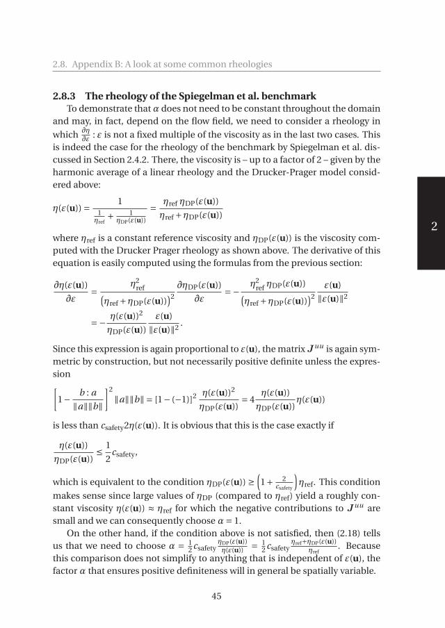
530578-L-sub01-bw-Fraters530578-L-sub01-bw-Fraters530578-L-sub01-bw-Fraters530578-L-sub01-bw-FratersProcessed on: 10-4-2019Processed on: 10-4-2019Processed on: 10-4-2019Processed on: 10-4-2019 PDF page: 55PDF page: 55PDF page: 55PDF page: 55
2
2.8. Appendix B: A look at some common rheologies
2.8.3 The rheology of the Spiegelman et al. benchmarkTo demonstrate that α does not need to be constant throughout the domain
and may, in fact, depend on the flow field, we need to consider a rheology in
which ∂η∂ε : ε is not a fixed multiple of the viscosity as in the last two cases. This
is indeed the case for the rheology of the benchmark by Spiegelman et al. dis-cussed in Section 2.4.2. There, the viscosity is – up to a factor of 2 – given by theharmonic average of a linear rheology and the Drucker-Prager model consid-ered above:
η(ε(u)) = 11
ηref+ 1
ηDP(ε(u))
= ηref ηDP(ε(u))
ηref +ηDP(ε(u))
where ηref is a constant reference viscosity and ηDP(ε(u)) is the viscosity com-puted with the Drucker Prager rheology as shown above. The derivative of thisequation is easily computed using the formulas from the previous section:
∂η(ε(u))
∂ε= η2
ref(ηref +ηDP(ε(u))
)2 ∂ηDP(ε(u))
∂ε=− η2
ref ηDP(ε(u))(ηref +ηDP(ε(u))
)2 ε(u)
‖ε(u)‖2
=− η(ε(u))2
ηDP(ε(u))
ε(u)
‖ε(u)‖2 .
Since this expression is again proportional to ε(u), the matrix Juu is again sym-metric by construction, but not necessarily positive definite unless the expres-sion[
1− b : a
‖a‖‖b‖]2
‖a‖‖b‖ = [1− (−1)]2 η(ε(u))2
ηDP(ε(u))= 4
η(ε(u))
ηDP(ε(u))η(ε(u))
is less than csafety2η(ε(u)). It is obvious that this is the case exactly if
η(ε(u))
ηDP(ε(u))≤ 1
2csafety,
which is equivalent to the condition ηDP(ε(u)) ≥(1+ 2
csafety
)ηref. This condition
makes sense since large values of ηDP (compared to ηref) yield a roughly con-stant viscosity η(ε(u)) ≈ ηref for which the negative contributions to Juu aresmall and we can consequently choose α= 1.
On the other hand, if the condition above is not satisfied, then (2.18) tellsus that we need to choose α = 1
2 csafetyηDP(ε(u))η(ε(u)) = 1
2 csafetyηref+ηDP(ε(u))
ηref. Because
this comparison does not simplify to anything that is independent of ε(u), thefactor α that ensures positive definiteness will in general be spatially variable.
45
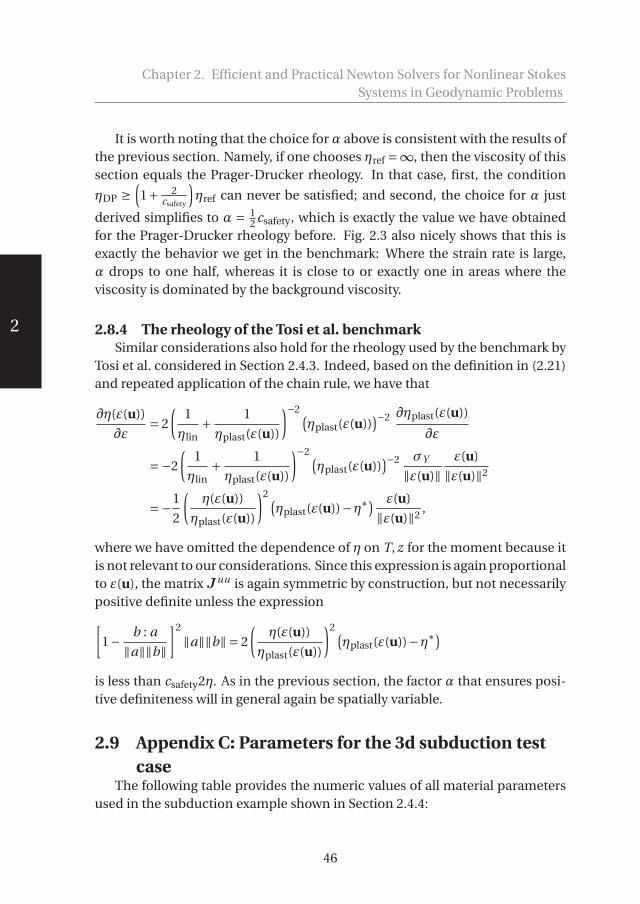
530578-L-sub01-bw-Fraters530578-L-sub01-bw-Fraters530578-L-sub01-bw-Fraters530578-L-sub01-bw-FratersProcessed on: 10-4-2019Processed on: 10-4-2019Processed on: 10-4-2019Processed on: 10-4-2019 PDF page: 56PDF page: 56PDF page: 56PDF page: 56
2
Chapter 2. Efficient and Practical Newton Solvers for Nonlinear StokesSystems in Geodynamic Problems
It is worth noting that the choice for α above is consistent with the results ofthe previous section. Namely, if one chooses ηref =∞, then the viscosity of thissection equals the Prager-Drucker rheology. In that case, first, the condition
ηDP ≥(1+ 2
csafety
)ηref can never be satisfied; and second, the choice for α just
derived simplifies to α = 12 csafety, which is exactly the value we have obtained
for the Prager-Drucker rheology before. Fig. 2.3 also nicely shows that this isexactly the behavior we get in the benchmark: Where the strain rate is large,α drops to one half, whereas it is close to or exactly one in areas where theviscosity is dominated by the background viscosity.
2.8.4 The rheology of the Tosi et al. benchmarkSimilar considerations also hold for the rheology used by the benchmark by
Tosi et al. considered in Section 2.4.3. Indeed, based on the definition in (2.21)and repeated application of the chain rule, we have that
∂η(ε(u))
∂ε= 2
(1
ηlin+ 1
ηplast(ε(u))
)−2 (ηplast(ε(u))
)−2 ∂ηplast(ε(u))
∂ε
=−2
(1
ηlin+ 1
ηplast(ε(u))
)−2 (ηplast(ε(u))
)−2 σY
‖ε(u)‖ε(u)
‖ε(u)‖2
=−1
2
(η(ε(u))
ηplast(ε(u))
)2 (ηplast(ε(u))−η∗
) ε(u)
‖ε(u)‖2 ,
where we have omitted the dependence of η on T, z for the moment because itis not relevant to our considerations. Since this expression is again proportionalto ε(u), the matrix Juu is again symmetric by construction, but not necessarilypositive definite unless the expression[
1− b : a
‖a‖‖b‖]2
‖a‖‖b‖ = 2
(η(ε(u))
ηplast(ε(u))
)2 (ηplast(ε(u))−η∗
)is less than csafety2η. As in the previous section, the factor α that ensures posi-tive definiteness will in general again be spatially variable.
2.9 Appendix C: Parameters for the 3d subduction testcase
The following table provides the numeric values of all material parametersused in the subduction example shown in Section 2.4.4:
46

530578-L-sub01-bw-Fraters530578-L-sub01-bw-Fraters530578-L-sub01-bw-Fraters530578-L-sub01-bw-FratersProcessed on: 10-4-2019Processed on: 10-4-2019Processed on: 10-4-2019Processed on: 10-4-2019 PDF page: 57PDF page: 57PDF page: 57PDF page: 57
2.9. Appendix C: Parameters for the 3d subduction test case
thermal conductivity (W m−1 K−1) 4specific heat capacity (J kg−1 K−1) 1250
reference temperature (K) 273.0reference densities (kg) 3300
initial viscosity (Pa s) 1020
cohesion C (Pa) 20 ·106
angle of internal friction φ (°) 30dislocation stress exponent ndisl 3
dislocation prefactor Adisl (Pa−n s−1) 3.12504 ·10−14
dislocation activation energy Edisl (J mol−1) 4.3 ·105
dislocation activation volume Vdisl (m−3 mol−1) 25 ·10−6
diffusion stress exponent ndiff 1diffusion prefactor Adiff (Pa−n s−1) 1.92 ·10−11
diffusion activation energy Ediff (J mol−1) 335 ·103
diffusion activation volume Vdiff (m−3 mol−1) 4 ·10−6
minimum viscosity ηmin (Pa s) 1019
maximum viscosity ηmax (Pa s) 1024
In addition, we choose dimensionless scaling factors νdisl = νdiff = 1 in theupper mantle, and νdisl = νdiff = 100 in the lower mantle.
47

530578-L-sub01-bw-Fraters530578-L-sub01-bw-Fraters530578-L-sub01-bw-Fraters530578-L-sub01-bw-FratersProcessed on: 10-4-2019Processed on: 10-4-2019Processed on: 10-4-2019Processed on: 10-4-2019 PDF page: 58PDF page: 58PDF page: 58PDF page: 58
530578-L-sub01-bw-Fraters530578-L-sub01-bw-Fraters530578-L-sub01-bw-Fraters530578-L-sub01-bw-FratersProcessed on: 10-4-2019Processed on: 10-4-2019Processed on: 10-4-2019Processed on: 10-4-2019 PDF page: 59PDF page: 59PDF page: 59PDF page: 59
3The Geodynamic World Builder: a solution forcomplex initial conditions in numericalmodelling

530578-L-sub01-bw-Fraters530578-L-sub01-bw-Fraters530578-L-sub01-bw-Fraters530578-L-sub01-bw-FratersProcessed on: 10-4-2019Processed on: 10-4-2019Processed on: 10-4-2019Processed on: 10-4-2019 PDF page: 60PDF page: 60PDF page: 60PDF page: 60
3
Chapter 3. The Geodynamic World Builder: a solution for complex initialconditions in numerical modelling
3.1 AbstractThe Geodynamic World Builder is an open source code library intended to
set up initial conditions for computational geodynamic models in both Carte-sian and Spherical geometries. The inputs for the JSON-style parameter fileare not mathematical, but rather a structured nested list describing tectonicfeatures, e.g. a continental, an oceanic or a subducting plate. Each of these tec-tonic features can be assigned a specific temperature profile (e.g. plate model)or composition label (e.g. uniform). For each point in space, the GeodynamicWorld Builder can return the composition and/or temperature. It is written inC++, but can be used in almost any language through its C and Fortran wrap-pers. Various examples of 2D and 3D subduction settings are presented. TheWorld builder comes with an extensive online User Manual.
3.2 IntroductionGeodynamic modelling has been used in the past four decades to help us
better understand the physical processes of Earth’s interior including large-scale mantle convection and plate tectonics, or detailed processes of crustal de-formation. Numerical modelling of geodynamic processes involves solving thepertinent partial differential equations (PDEs) of mass, momentum and energyconservation supplemented with rheological laws, material parameters andwith an equation of thermodynamic state relating, e.g., density, temperatureand pressure (e.g. Gerya, 2010; Schubert et al., 2001). In addition these PDEsmust be constrained by boundary conditions, which can be time-dependent,and by initial conditions which describe the starting model for solving the geo-dynamic problem at hand. For example, 3D initial models of a geometricallysimplified nature are often constructed for modelling of generic subductionevolution using plate boundaries and lithosphere domains that are parallel tothe sides of the (rectangular) model domain (e.g. Yamato et al., 2009; Stegmanet al., 2010b; Brune and Autin, 2013; Schellart and Moresi, 2013; Duretz et al.,2014; Holt et al., 2015; Leng and Gurnis, 2015; Naliboff and Buiter, 2015; Ki-raly et al., 2016; Schellart, 2017). When numerically simulating (regions of) theEarth, geometrically more complex initial models are required, e.g., involving
This paper has been submitted to Solid Earth as The Geodynamic World Builder: a solutionfor complex initial conditions in numerical modelling, M. Fraters, C. Thieulot, A. van den Bergand W. Spakman.
50
530578-L-sub01-bw-Fraters530578-L-sub01-bw-Fraters530578-L-sub01-bw-Fraters530578-L-sub01-bw-FratersProcessed on: 10-4-2019Processed on: 10-4-2019Processed on: 10-4-2019Processed on: 10-4-2019 PDF page: 61PDF page: 61PDF page: 61PDF page: 61
3
3.3. Geodynamic World Builder Philosophy
the starting plate-tectonic layout, initial trench geometry and slab shape foruse either instantaneous dynamics modelling or as initial model for modellingof subduction evolution (e.g. Alisic et al., 2012; Liu and Stegman, 2011; Jadamecand Billen, 2010, 2012; Chertova et al., 2014a; Billen and Arredondo, 2018; Zhouet al., 2018). Such initial model setups cannot be easily created, adapted, orshared with the community, nor easily transferred to another code. We presentin this paper a solution to these problems in the form of an open source codelibrary, the Geodynamic World Builder, which has been designed to be user-friendly, extensible, and portable across different platforms. We present thefirst stable version of the World Builder which focuses on creating geometricallycomplex 3D initial models (geometry, composition, and temperature) consist-ing of first-order plate tectonic features such as continental and oceanic plates,oceanic ridges and transform faults and 3D lithosphere subduction. These con-figured initial models are intended to help advance research into simulations ofinstantaneous dynamic modelling and of plate tectonic evolution with a widerange of geometric complexity.
3.3 Geodynamic World Builder Philosophy3.3.1 User Philosophy
In this section we describe the philosophy of how tectonic features such asplates, ridges, faults and slabs can be parameterized by lines and areas that im-plicitly define volumes to which temperature and composition can be assigned.A composition is a part of the model that is assigned a particular identifying la-bel and in addition an indicator which is given a value between 0 and 1. Thisindicator can be used by codes using the GWB output to ascribe physical prop-erties to different model regions.
To minimize user effort, the Geodynamic World Builder (GWB) utilizes a pa-rameterization of 3D structures by 2D coordinate input, by defining their (pro-jected) location on the surface. The GWB can be used to create initial modelsin Cartesian and spherical geometries.
User input files should be specified in JSON (json.org), which is aninternationally standardized language (ISO/IEC 21778). We use a relaxedform of JSON which allows comments, NaN’s and tailing commas to im-prove usability through RapidJSON (http://rapidjson.org/). The user in-puts coordinates and can assign particular properties to features such as ’lin-ear’ for a temperature profile, or ’uniform’ for the compositional makeup ofthe plate. Note that only a subset of the options is mentioned in this pa-per. We refer to the online Geodynamic World Builder Manual (https://geodynamicworldbuilder.github.io) for the complete listing.
51

530578-L-sub01-bw-Fraters530578-L-sub01-bw-Fraters530578-L-sub01-bw-Fraters530578-L-sub01-bw-FratersProcessed on: 10-4-2019Processed on: 10-4-2019Processed on: 10-4-2019Processed on: 10-4-2019 PDF page: 62PDF page: 62PDF page: 62PDF page: 62
3
Chapter 3. The Geodynamic World Builder: a solution for complex initialconditions in numerical modelling
The GWB uses a hierarchical overlay of features. This means that featuresdefined first are spatially overlain by features defined later in places where bothoverlap. The GWB recognizes two types of features: area features and line fea-tures, which will be explained in the following sections. A possible third type offeatures, point features, will be discussed in section 3.5.
Continental lithosphere plateA continental plate is an ’area feature’ in the GWB and is defined by its sur-
face perimeter and its thickness. The perimeter is specified as a list of pointswhich enclose the continental area. Within the defined volume of the conti-nental plate, the GWB offers various options for defining temperature valuesand compositions. For example, a continental plate can be assigned multiplelayers of different compositions and a linear geotherm that matches a prede-fined adiabatic mantle temperature at the base of the lithosphere. We note thatcontinental lithosphere with a variable thickness is a development for futurereleases of the GWB, but can be mimicked in the present version by specifyingcontiguous continental areas with different thickness. Also, continental topog-raphy is currently not explicitly implemented, but it can be achieved througha sticky air approach, where air is a composition of varying thickness atop themodel (Schmeling et al., 2008; Crameri et al., 2012).
Oceanic lithosphere plateLike the continental plate, the oceanic plate is parameterized as an area fea-
ture with a flat surface. We have implemented the ’plate model’ (e.g. Fowler,2005) for assigning an age-dependent temperature to oceanic lithosphere. Insection 3.4.1 we will show an example of a ridge-transform system with ridgejumps. The workaround for implementing oceanic bathymetry is the same asfor the continental lithosphere plate.
The mantleThe upper and lower mantle can also be parameterized as an area feature
that starts below the lithosphere or at the surface and is overlain by lithospherein a later building stage. This allows for defining a upper and lower mantle andto insert specific volumetric structures such as Large Low Shear wave VelocityProvinces (LLSVPs) at the core-mantle boundary. In the present version thesemantle features can be assigned a radially uniform, linear or adiabatic tem-perature profile. Future versions may include laterally varying temperature orcompositions, e.g. scaled from seismic tomography models (e.g. Steinbergeret al., 2015).
52

530578-L-sub01-bw-Fraters530578-L-sub01-bw-Fraters530578-L-sub01-bw-Fraters530578-L-sub01-bw-FratersProcessed on: 10-4-2019Processed on: 10-4-2019Processed on: 10-4-2019Processed on: 10-4-2019 PDF page: 63PDF page: 63PDF page: 63PDF page: 63
3
3.3. Geodynamic World Builder Philosophy
A subducting plateA subducting plate is a ’line feature’ in the GWB and is defined by the lo-
cation of the trench and one or more depth segments each describing a partof the geometry of the subducting slab. They are defined by a length and bythicknesses and dip angles at beginning and end of the slab segment. In se-quence, these segments can makeup a smoothly varying slab geometry whichcan for example flatten in the upper mantle transition zone, or may prescribea slab entering the lower mantle. Every point in the trench coordinate list de-fines a vertical section of the subducting plate that may consist of one or sev-eral slab segments. Both sections and segments can vary in length, dip an-gle or thickness. The length of a subducting slab is always computed as thelength along the top of the slab so that this can straightforwardly represent theamount of relative plate convergence during a certain period. The dip angle isdefined as the angle between the surface and the local plunge of the slab. Thedip angle is specified at the start and end point of each depth segment alongthe vertical section. Dip angles are linearly interpolated along a segment. Theoverall direction of slab dip can be to either side of the trench and is selectedby specifying for each subducting plate an additional point at the surface, the’dip-point’, at the slab dip-side of the trench segment. Slab dip is linearly in-terpolated between subsequent vertical slab segments. This parameterizationallows for constructing smoothly varying 3D slab morphology. Note that it isalso possible to give slabs a starting depth to configure detached slabs.
For each point at the surface of the slab the depth and the distance to thetrench, as measured along the surface, are available and can be used to assignslab temperatures, e.g., by using the McKenzie (1970) slab temperature model.
A faultTo allow for complicated fault shapes (e.g. listric faults), faults are also pa-
rameterized as line features. An important difference between faults and sub-ducting plates is that for subducting plates the trench defines the top of theplate at the plate boundary, while for faults the line feature defines the centerof the fault with respect to which a fault thickness can be defined.
3.3.2 Code philosophyThe following design principles define the Geodynamic World Builder:
1. A single text-based input file centered around plate tectonic terminology:as explained in Section 3.3.1. The particular syntax is specified in theonline manual and will be illustrated with examples below.
53

530578-L-sub01-bw-Fraters530578-L-sub01-bw-Fraters530578-L-sub01-bw-Fraters530578-L-sub01-bw-FratersProcessed on: 10-4-2019Processed on: 10-4-2019Processed on: 10-4-2019Processed on: 10-4-2019 PDF page: 64PDF page: 64PDF page: 64PDF page: 64
3
Chapter 3. The Geodynamic World Builder: a solution for complex initialconditions in numerical modelling
2. Code-, language-, and platform-independence: The GWB is designed tobe integrated in the different geodynamic codes through a simple inter-face. The library is written in C++, has official interfaces (wrappers) to Cand Fortran and it is possible to call the GWB from the command line.Note that the C wrapper enables calling the GWB from almost any otherlanguage like Python and Matlab. The code is continuously tested withevery change on the Linux, OSX and Windows operating systems.
3. Up-to-date user manual and code documentation. Manual and doxygenhttp://doxygen.nl/ code documentation provided through https://geodynamicworldbuilder.github.io.
4. Safe use in parallel codes: The GWB is split into two phases. The setupphase, encapsulated in the function create_world, is not thread safe butupon completion the generated "world object" is thread-safe and can beused to query temperature and compositions in parallel.
5. Readable and extensible code: Following ASPECT (Kronbichler et al.,2012; Heister et al., 2017) we use a plugin system for different parts ofthe code. Such plugins enable users to add functionalities such as platetectonic features or coordinate systems without knowledge of the rest ofthe code.
6. Version numbering: using Semantic Versioning 2.0.0 (https://semver.org). The input file should specify the major version number that mustmatch the version number of the used GWB. Before the release of ma-jor version 1, backwards incompatible changes may be made in minorversions, because they will be beta releases. This implies that the inputfiles for major version 0 also must contain the minor version number. Allthese features help ensuring reproducibility of results.
3.4 Using the World BuilderTo exemplify input files and to show the capabilities of the Geodynamic
World Builder, we show here three 2D examples, and two 3D examples of theGWB visualized through the standalone visualization application. This appli-cation creates so-called vtu files which can be visualized by programs like Par-aview (paraview.org). Furthermore, we show examples of GWB use with theSEPRAN (van den Berg et al., 2015), ELEFANT (Plunder et al., 2018) and AS-PECT codes. The annotated input files to create these models are presented inappendixes 3.8 to 3.13 and are part of the GWB repository.
54
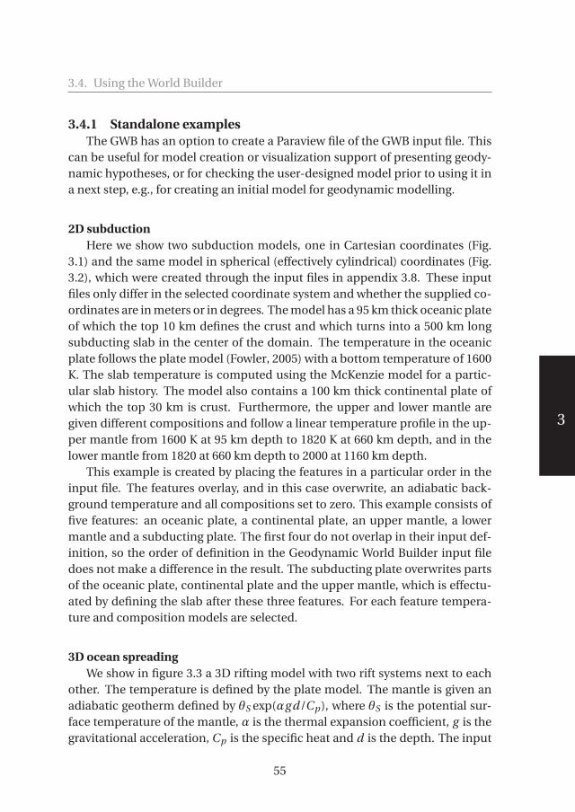
530578-L-sub01-bw-Fraters530578-L-sub01-bw-Fraters530578-L-sub01-bw-Fraters530578-L-sub01-bw-FratersProcessed on: 10-4-2019Processed on: 10-4-2019Processed on: 10-4-2019Processed on: 10-4-2019 PDF page: 65PDF page: 65PDF page: 65PDF page: 65
3
3.4. Using the World Builder
3.4.1 Standalone examplesThe GWB has an option to create a Paraview file of the GWB input file. This
can be useful for model creation or visualization support of presenting geody-namic hypotheses, or for checking the user-designed model prior to using it ina next step, e.g., for creating an initial model for geodynamic modelling.
2D subductionHere we show two subduction models, one in Cartesian coordinates (Fig.
3.1) and the same model in spherical (effectively cylindrical) coordinates (Fig.3.2), which were created through the input files in appendix 3.8. These inputfiles only differ in the selected coordinate system and whether the supplied co-ordinates are in meters or in degrees. The model has a 95 km thick oceanic plateof which the top 10 km defines the crust and which turns into a 500 km longsubducting slab in the center of the domain. The temperature in the oceanicplate follows the plate model (Fowler, 2005) with a bottom temperature of 1600K. The slab temperature is computed using the McKenzie model for a partic-ular slab history. The model also contains a 100 km thick continental plate ofwhich the top 30 km is crust. Furthermore, the upper and lower mantle aregiven different compositions and follow a linear temperature profile in the up-per mantle from 1600 K at 95 km depth to 1820 K at 660 km depth, and in thelower mantle from 1820 at 660 km depth to 2000 at 1160 km depth.
This example is created by placing the features in a particular order in theinput file. The features overlay, and in this case overwrite, an adiabatic back-ground temperature and all compositions set to zero. This example consists offive features: an oceanic plate, a continental plate, an upper mantle, a lowermantle and a subducting plate. The first four do not overlap in their input def-inition, so the order of definition in the Geodynamic World Builder input filedoes not make a difference in the result. The subducting plate overwrites partsof the oceanic plate, continental plate and the upper mantle, which is effectu-ated by defining the slab after these three features. For each feature tempera-ture and composition models are selected.
3D ocean spreadingWe show in figure 3.3 a 3D rifting model with two rift systems next to each
other. The temperature is defined by the plate model. The mantle is given anadiabatic geotherm defined by θS exp(αg d/Cp ), where θS is the potential sur-face temperature of the mantle, α is the thermal expansion coefficient, g is thegravitational acceleration, Cp is the specific heat and d is the depth. The input
55

530578-L-sub01-bw-Fraters530578-L-sub01-bw-Fraters530578-L-sub01-bw-Fraters530578-L-sub01-bw-FratersProcessed on: 10-4-2019Processed on: 10-4-2019Processed on: 10-4-2019Processed on: 10-4-2019 PDF page: 66PDF page: 66PDF page: 66PDF page: 66
3
Chapter 3. The Geodynamic World Builder: a solution for complex initialconditions in numerical modelling
Figure 3.1: The top figure shows the distribution of different compositions through the modeldomain. The oceanic crust composition is light blue, the oceanic lithosphere is dark blue, thecontinental crust is light green, the continental lithosphere is dark green, the upper mantle islight red and the lower mantle dark red. The bottom figure shows the temperature distributionin the model (in Kelvin).
file of this example consists of the definition of the mantle domain followed bytwo oceanic plates, which form the two ridge-plate systems. The two oceanicplates are exactly the same, except for the shifted ridge location. The input filefor this example can be found in Appendix 3.9.
3D subductionFigure 3.4 shows a 3D example defining a subduction geometry similar to
the one in Plunder et al. (2018). In this example the trench consists of threeconnected straight lines. To create a smooth transition between these sections,the user can choose to use a monotone spline interpolation between the co-ordinates given by the user. This example includes a linear temperature upperand lower mantle as described in the 2D subduction example. The 95 km thickoceanic plate and the 120 km thick continental plate features are both definedbefore the subducting plate feature, of which the trench is defined along theinterface between the two. The slab itself is 95 km thick and consists of four
56

530578-L-sub01-bw-Fraters530578-L-sub01-bw-Fraters530578-L-sub01-bw-Fraters530578-L-sub01-bw-FratersProcessed on: 10-4-2019Processed on: 10-4-2019Processed on: 10-4-2019Processed on: 10-4-2019 PDF page: 67PDF page: 67PDF page: 67PDF page: 67
3
3.4. Using the World Builder
Figure 3.2: The same as setup as in figure 3.1, but now in spherical geometry. The top figureshows the composition, the bottom figure shows the temperature.
Figure 3.3: The temperature field of the 3D two rift systems example. Material with a temperaturebelow 950 K has been omitted, in order to better show the rifts. Note the second rift system inthe background.
57

530578-L-sub01-bw-Fraters530578-L-sub01-bw-Fraters530578-L-sub01-bw-Fraters530578-L-sub01-bw-FratersProcessed on: 10-4-2019Processed on: 10-4-2019Processed on: 10-4-2019Processed on: 10-4-2019 PDF page: 68PDF page: 68PDF page: 68PDF page: 68
3
Chapter 3. The Geodynamic World Builder: a solution for complex initialconditions in numerical modelling
Figure 3.4: The temperature field of the 3D subduction example. Note the smooth transitionbetween the upper and lower part of the subduction system in the top figure and the curvedgeometry of the slab in the lower figure. For visualization purposes we have omitted the top 25km of the model in the top figure.
segments. One 200 km long segment which goes from a dip angle of 0◦ to 45◦,and one 400 km long segment which has an angle of 45◦, one 200 km long seg-ment which goes from 45◦ to 0◦ and one 100 km long segment, with constantdip angle of 0◦. The input file for this example can be found in Appendix 3.10.
3.4.2 Using the GWB with SEPRANSEPRAN is a general purpose finite element toolkit applied in engineering
problems as well as in development of 2D and 3D numerical models in geody-namics and planetary science (Chertova et al., 2012, 2014a; Cížková et al., 2012;van den Berg et al., 2015, 2019; Zhao et al., 2019). The model contains a litho-spheric slab subducting under an overriding plate as shown in Fig. 3.5. Onesided subduction is obtained in a self consistent way by the presence of a weakcrustal layer of uniform viscosity 1021 Pa·s as part of the top of the subducting
58

530578-L-sub01-bw-Fraters530578-L-sub01-bw-Fraters530578-L-sub01-bw-Fraters530578-L-sub01-bw-FratersProcessed on: 10-4-2019Processed on: 10-4-2019Processed on: 10-4-2019Processed on: 10-4-2019 PDF page: 69PDF page: 69PDF page: 69PDF page: 69
3
3.4. Using the World Builder
lithosphere. The mantle underlying the crust has a temperature and pressuredependent viscosity with an Arrhenius type parameterization representative ofdiffusion creep in olivine under upper mantle pressure and temperature con-ditions. Viscosity is modeled as a material property for the crustal layer mate-rial and the mantle material. Material transport is implemented using particletracers that are advected by the convective flow. The medium is described as amechanical mixture of materials with contrasting properties.
A 2D rectangular domain of 1000 km depth and 2000 km width is used. Theinitial thermal and composition state is created using the Fortran wrapper ofthe GWB library. The GWB tool is called in a loop over all nodal points of theFEM mesh to define the initial temperature field for the subsequent convectioncalculations. In a similar way the material distribution of the initial state is de-fined by calling the composition function of the GWB library in a program loopover particle tracers. The input file for this example can be found in Appendix3.11.
3.4.3 Using the GWB with ELEFANTELEFANT is a 2D/3D Finite Element code for geodynamic problems (Maf-
fione et al., 2015; Lavecchia et al., 2017; Thieulot, 2017; Plunder et al., 2018)written in Fortran. It principally relies on bi/tri-linear velocity-constant pres-sure elements and uses the Marker-in-Cell technique to track materials. In or-der to demonstrate the GWB flexibility of use a 3D double subduction setupwas created with the Fortran wrapper of the GWB (see Fig. 3.6): a compositionbetween 1 and 6 was then easily assigned to all markers (two different oceaniccrusts and oceanic lithospheres, one upper mantle and one lower mantle) anda temperature based on the McKenzie model (McKenzie, 1970) was prescribedonto the FE mesh, as shown in Fig. 3.7.
The domain is a Cartesian box with dimensions 2000×2000×800 km and theFinite Element mesh counts 120×120×50 = 720,000 elements. Each elementcontains 64 randomly distributed markers. Free slip boundary conditions areimposed at the bottom (z = 0), top (z = Lz ) and sides (y = 0 and y = Ly ) ofthe domain. The other two sides, x = 0 and x = Lx , are a mix of free slip (forz < 100km or z > 690km) and open boundary conditions (for 100 < z < 690 km)(Chertova et al., 2012). The input file for this example can be found in Appendix3.12.
3.4.4 Using the GWB with ASPECTASPECT is an open source community FEM designed for geodynamic prob-
lems (Heister et al., 2017; Kronbichler et al., 2012). The model which was run
59
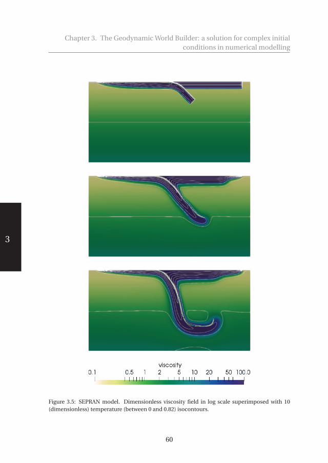
530578-L-sub01-bw-Fraters530578-L-sub01-bw-Fraters530578-L-sub01-bw-Fraters530578-L-sub01-bw-FratersProcessed on: 10-4-2019Processed on: 10-4-2019Processed on: 10-4-2019Processed on: 10-4-2019 PDF page: 70PDF page: 70PDF page: 70PDF page: 70
3
Chapter 3. The Geodynamic World Builder: a solution for complex initialconditions in numerical modelling
Figure 3.5: SEPRAN model. Dimensionless viscosity field in log scale superimposed with 10(dimensionless) temperature (between 0 and 0.82) isocontours.
60

530578-L-sub01-bw-Fraters530578-L-sub01-bw-Fraters530578-L-sub01-bw-Fraters530578-L-sub01-bw-FratersProcessed on: 10-4-2019Processed on: 10-4-2019Processed on: 10-4-2019Processed on: 10-4-2019 PDF page: 71PDF page: 71PDF page: 71PDF page: 71
3
3.4. Using the World Builder
1 do im=1 ,nmarker2 depth=Lz−zm(im)3 do imat =1 ,nmat4 c a l l composition_3d ( cworld ,xm(im) ,&5 ym(im) ,zm(im) ,&6 depth , imat−1, f l a g )7 i f ( f l a g ==imat ) then8 mat(im) =imat9 e x i t
10 end i f11 end do12 end do13
14 do ip =1 ,np15 depth=Lz−z ( ip )16 c a l l temperature_3d ( cworld , x ( ip ) , y ( ip ) ,&17 z ( ip ) , depth , gz , T( ip ) )18 end do
Figure 3.6: Example ELEFANT query routine using the GWB supplied Fortran wrappers compo-sition_3d() and temperature_3d(): a) a loop runs over all markers and determines for each thecomposition at its location; b) a loop runs over all grid points and the GWB returns its tempera-ture as a function of their spatial coordinates.
with ASPECT is a 3D Cartesian model of a curved subduction system similarto the plate-tectonic setting of the Lesser Antilles subduction of the easternCaribbean region. The lithosphere consists of a strong zero velocity Caribbeanupper plate, surrounded by an oceanic North American plate to the north andnortheast and the oceanic-continental South American plate to the south andsoutheast. In the model the North American and South American plates movewest at a average rate over the past 5 Ma of 1.4 cm/yr relative to the Caribbeanplate (Boschman et al., 2014). The Lesser Antilles trench curves around the eastand north of the Caribbean plate. To the south, the Caribbean plate is partiallydecoupled from the South American plate by a 50 km wide weak zone. To thenorthwest a 250 km wide weak zone, from the western end of the trench to thewestern edge of the model, partially decouples the North American plate fromthe Caribbean plate. Below the lithosphere the sidewalls are open (Chertovaet al., 2012, 2014a) allowing for horizontal in/out flow of mantle material. From660 km down a denser and more viscous material has been prescribed to delaysinking of the slab into the lower mantle. The top boundary is a free surface
61
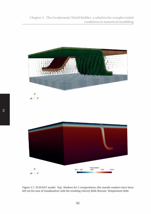
530578-L-sub01-bw-Fraters530578-L-sub01-bw-Fraters530578-L-sub01-bw-Fraters530578-L-sub01-bw-FratersProcessed on: 10-4-2019Processed on: 10-4-2019Processed on: 10-4-2019Processed on: 10-4-2019 PDF page: 72PDF page: 72PDF page: 72PDF page: 72
3
Chapter 3. The Geodynamic World Builder: a solution for complex initialconditions in numerical modelling
Figure 3.7: ELEFANT model. Top: Markers for 5 compositions (the mantle markers have beenleft out for ease of visualization) with the resulting velocity field; Bottom: Temperature field.
62

530578-L-sub01-bw-Fraters530578-L-sub01-bw-Fraters530578-L-sub01-bw-Fraters530578-L-sub01-bw-FratersProcessed on: 10-4-2019Processed on: 10-4-2019Processed on: 10-4-2019Processed on: 10-4-2019 PDF page: 73PDF page: 73PDF page: 73PDF page: 73
3
3.4. Using the World Builder
Figure 3.8: The 3D ASPECT Caribbean example after 2.5 million years of evolution. The topimage is a top view of the model, where the top 50 km is removed, and where the viscosity field isshown with the velocity field indicated by the arrows. The bottom two figures are cut outs of thetemperature field between 600 K and 1535 K, showing in colour the temperature (T) and witharrows the velocity fields, highlighting the velocity field in the slab and lithosphere.
(Rose et al., 2017) and the bottom boundary has a prescribed zero velocity. Theresult of about 2.5 million years of evolution is shown in figure 3.8.
The details of the setup are presented in Appendix 3.13.
63
530578-L-sub01-bw-Fraters530578-L-sub01-bw-Fraters530578-L-sub01-bw-Fraters530578-L-sub01-bw-FratersProcessed on: 10-4-2019Processed on: 10-4-2019Processed on: 10-4-2019Processed on: 10-4-2019 PDF page: 74PDF page: 74PDF page: 74PDF page: 74
3
Chapter 3. The Geodynamic World Builder: a solution for complex initialconditions in numerical modelling
3.4.5 PerformanceThe Finite Element mesh used in the example of section 3.4.4 is built in sev-
eral steps by ASPECT: the code starts with a regular grid and allows adaptivemesh refinement to take place one level at the time. Each step of this processcalls the GWB library. The first step generates a grid counting 28,000 elementsand reports a total setup time for the initial conditions of 3.6 seconds on 480MPI processes. The second step mesh counts 99,000 elements while the setupof the initial conditions took (cumulatively) 10 seconds. The third step sees thenumber of element jump to about 560,000 elements while its total (cumula-tive) time to setup the initial conditions remains low at about 36 seconds. Thisfigure represents about 0.7% of the total wall time of the first time step, and anegligible portion of the total wall time of the 20Myr-long simulation.
3.5 DiscussionWe presented the Geodynamic World Builder Version 0.2.0 as a tool for con-
structing 2D and 3D initial models of geodynamic settings involving crust/litho-sphere, plate boundaries, and subduction. The interface of the GWB with anumerical modelling code is based on a query of the modelling code to sup-ply temperature, density, or other information at a particular position. Thispaper discusses version 0.2.0 of the Geodynamic World Builder, which is con-sidered to be a beta version of the code. Input format and/or functionality maychange between minor versions and this will be documented on the website.From version 1.0.0, we will use Semantic Versioning 2.0.0 (https://semver.org/spec/v2.0.0.html), and backwards incompatible changes will only bemade in every major version of the code. Future improvements may for ex-ample include extra temperature or composition modules, e.g. derived fromtomographic models, new or improved features or even new output interfaces,e.g. velocity boundary conditions or initial topography. As an extension to areaand line features, adding point features are another possible improvement tothe Geodynamic World Builder. These can represent, for example, a sphericalweak seed or a plume. Because of a simple query interface it is in principle pos-sible to use the GWB in connection with existing numerical modelling codesused by the geodynamic community. The use of the GWB can also just be re-stricted to creating 2D or 3D geodynamic models/cartoons for, e.g., teachingpurposes or for illustrating a complex geodynamic setting.
3.6 Code availabilityThe code is freely available at https://geodynamicworldbuilder.github.
io under licence LGPLv2.1. All examples presented in this work are available ascookbooks in the code.
64

530578-L-sub01-bw-Fraters530578-L-sub01-bw-Fraters530578-L-sub01-bw-Fraters530578-L-sub01-bw-FratersProcessed on: 10-4-2019Processed on: 10-4-2019Processed on: 10-4-2019Processed on: 10-4-2019 PDF page: 75PDF page: 75PDF page: 75PDF page: 75
3
3.7. Acknowledgements
3.7 AcknowledgementsM.F. acknowledges constructive feedback from the ASPECT community,
and especially from T. Heister, W. Bangerth and R. Gassmöller. The authorsalso acknowledge constructive proofreading by R. Myhill, H. Brett and L. vande Wiel. MF and CT are indebted to the Computational Infrastructure for Geo-dynamics (CIG) for their recurring participation to the ASPECT hackathons,during which the foundation of this work was laid out. This work is fundedby the Netherlands Organization for Scientific Research (NWO), as part of theCaribbean Research program, grant 858.14.070 and partly supported by the Re-search Council of Norway through its Centres of Excellence funding scheme,project number 223272. Data visualization is carried out with ParaView soft-ware https://paraview.org/.
3.8 2D subduction examples3.8.1 Cartesian input file
1 {2 "version":"0.2",3 "cross section":[[0 ,0] ,[100 ,0]] ,4 "features":5 [6 // defining the oceanic plate7 {8 "model":"oceanic plate", "name":"oceanic plate",9 "coordinates":[[-1e3 ,-1e3] ,[1150e3 ,-1e3] ,[1150e3 ,1e3],[-1e3 ,1e3]],
10 "temperature models":11 [12 {"model":"plate model", "max depth":95e3, "bottom temperature":1600 ,13 "spreading velocity":0.005 ,14 "ridge coordinates":[[100e3 ,-1e3],[100e3 ,1e3]]}15 ],16 "composition models":17 [18 {"model":"uniform", "compositions":[0], "max depth":10e3},19 {"model":"uniform", "compositions":[1], "min depth":10e3,20 "max depth":95e3}21 ]22 },23 // defining a continental plate24 {25 "model":"continental plate", "name":"continental plate",26 "coordinates":[[1150e3 ,-1e3] ,[2001e3 ,-1e3] ,[2001e3 ,1e3] ,[1150e3 ,1e3]],27 "temperature models":28 [29 {"model":"linear", "max depth":95e3, "bottom temperature":1600}30 ],31 "composition models":32 [33 {"model":"uniform", "compositions":[2], "max depth":30e3},34 {"model":"uniform", "compositions":[3], "min depth":30e3,35 "max depth":65e3}36 ]37 },38 // defining the upper mantle
65

530578-L-sub01-bw-Fraters530578-L-sub01-bw-Fraters530578-L-sub01-bw-Fraters530578-L-sub01-bw-FratersProcessed on: 10-4-2019Processed on: 10-4-2019Processed on: 10-4-2019Processed on: 10-4-2019 PDF page: 76PDF page: 76PDF page: 76PDF page: 76
3
Chapter 3. The Geodynamic World Builder: a solution for complex initialconditions in numerical modelling
39 {40 "model":"mantle layer", "name":"upper mantle",41 "min depth":95e3, "max depth":660e3,42 "coordinates":[[-1e3 ,-1e3] ,[2001e3 ,-1e3] ,[2001e3 ,1e3],[-1e3 ,1e3]],43 "temperature models":44 [45 {"model":"linear", "min depth":95e3, "max depth":660e3,46 "top temperature":1600, "bottom temperature":1820}47 ],48 "composition models":[{"model":"uniform", "compositions":[4]}]49 },50 // defining the lower mantle51 {52 "model":"mantle layer", "name":"lower mantle",53 "min depth":660e3, "max depth":1160e3 ,54 "coordinates":[[-1e3 ,-1e3] ,[2001e3 ,-1e3] ,[2001e3 ,1e3],[-1e3 ,1e3]],55 "temperature models":56 [57 {"model":"linear", "min depth":660e3, "max depth":1160e3,58 "top temperature":1820, "bottom temperature":2000}59 ],60 "composition models":[{"model":"uniform", "compositions":[5]}]61 },62 // defining the subducting plate dipping towards the continental plate63 {64 "model":"subducting plate", "name":"Subducting plate",65 "coordinates":[[1150e3 ,-1e3] ,[1150e3 ,1e3]], "dip point":[2000e3 ,0],66 "segments":[{"length":200e3 , "thickness":[95e3], "angle":[0 ,45]} ,67 {"length":200e3 , "thickness":[95e3], "angle":[45]} ,68 {"length":200e3 , "thickness":[95e3], "angle":[45,0]} ,69 {"length":100e3 , "thickness":[95e3], "angle":[0]}] ,70 "temperature models":7172 {"model":"plate model", "density":3300, "plate velocity":0.01 }73 ],74 "composition models":75 [76 {"model":"uniform", "compositions":[0], "max distance slab top":10e3},77 {"model":"uniform", "compositions":[1], "min distance slab top":10e3 ,78 "max distance slab top":95e3 }79 ]80 }81 ]82 }
Listing 3.1: 2D Cartesian subduction example. The lines of green text (preceded by the doubleforward slashes) are comments and have no effect on the result.
3.8.2 Spherical input file
1 {2 "version":"0.2",3 "cross section":[[0 ,0] ,[10 ,0]] ,4 "features":5 [6 // defining the oceanic plate7 {8 "model":"oceanic plate", "name":"oceanic plate",9 "coordinates":[[-1,-1],[11.5,-1],[11.5,1],[-1,1]],
10 "temperature models":11 [12 {"model":"plate model", "max depth":95e3, "bottom temperature":1600 ,13 "spreading velocity":0.005 ,14 "ridge coordinates":[[1 , -1] ,[1 ,1]]}
66

530578-L-sub01-bw-Fraters530578-L-sub01-bw-Fraters530578-L-sub01-bw-Fraters530578-L-sub01-bw-FratersProcessed on: 10-4-2019Processed on: 10-4-2019Processed on: 10-4-2019Processed on: 10-4-2019 PDF page: 77PDF page: 77PDF page: 77PDF page: 77
3
3.8. 2D subduction examples
15 ],16 "composition models":17 [18 {"model":"uniform", "compositions":[0], "max depth":10e3},19 {"model":"uniform", "compositions":[1], "min depth":10e3,20 "max depth":95e3}21 ]22 },23 // defining a continental plate24 {25 "model":"continental plate", "name":"continental plate",26 "coordinates":[[11.5 , -1] ,[21 , -1] ,[21 ,1] ,[11.5 ,1]] ,27 "temperature models":28 [29 {"model":"linear", "max depth":95e3, "bottom temperature":1600}30 ],31 "composition models":32 [33 {"model":"uniform", "compositions":[2], "max depth":30e3},34 {"model":"uniform", "compositions":[3], "min depth":30e3,35 "max depth":65e3}36 ]37 },38 // defining the upper mantle39 {40 "model":"mantle layer", "name":"upper mantle",41 "min depth":95e3, "max depth":660e3,42 "coordinates":[[-1,-1],[21,-1],[21,1],[-1,1]],43 "temperature models":44 [45 {"model":"linear", "min depth":95e3, "max depth":660e3,46 "top temperature":1600, "bottom temperature":1820}47 ],48 "composition models":[{"model":"uniform", "compositions":[4]}]49 },50 // defining the lower mantle51 {52 "model":"mantle layer", "name":"lower mantle",53 "min depth":660e3, "max depth":1160e3 ,54 "coordinates":[[-1,-1],[21,-1],[21,1],[-1,1]],55 "temperature models":56 [57 {"model":"linear", "min depth":660e3, "max depth":1160e3,58 "top temperature":1820, "bottom temperature":2000}59 ],60 "composition models":[{"model":"uniform", "compositions":[5]}]61 },62 // defining the subducting plate dipping towards the continental plate63 {64 "model":"subducting plate", "name":"Subducting plate",65 "coordinates":[[[11.5 , -1] ,[11.5 ,1]] , "dip point":[20,0],66 "segments":[{"length":200e3 , "thickness":[95e3], "angle":[0 ,45]} ,67 {"length":200e3 , "thickness":[95e3], "angle":[45]} ,68 {"length":200e3 , "thickness":[95e3], "angle":[45,0]} ,69 {"length":100e3 , "thickness":[95e3], "angle":[0]}] ,70 "temperature models":7172 {"model":"plate model", "density":3300, "plate velocity":0.01 }73 ],74 "composition models":75 [76 {"model":"uniform", "compositions":[0], "max distance slab top":10e3},77 {"model":"uniform", "compositions":[1], "min distance slab top":10e3 ,78 "max distance slab top":95e3 }79 ]
67

530578-L-sub01-bw-Fraters530578-L-sub01-bw-Fraters530578-L-sub01-bw-Fraters530578-L-sub01-bw-FratersProcessed on: 10-4-2019Processed on: 10-4-2019Processed on: 10-4-2019Processed on: 10-4-2019 PDF page: 78PDF page: 78PDF page: 78PDF page: 78
3
Chapter 3. The Geodynamic World Builder: a solution for complex initialconditions in numerical modelling
80 }81 ]82 }
Listing 3.2: 2D Spherical subduction example. The lines of green text (preceded by the doubleforward slashes) are comments and have no effect on the result.
3.9 3D ocean spreading example input file1 {2 "version":"0.2",3 "features":4 [5 // defining one of the oceanic plates with a ridge6 {7 "model":"oceanic plate", "name":"oceanic plate A",8 "coordinates":[[-1e3 ,-1e3] ,[2001e3 ,-1e3] ,[2001e3 ,1000e3],[-1e3 ,1000 e3]],9 "temperature models":
10 [11 {12 "model":"plate model", "max depth":95e3, "spreading velocity":0.005 ,13 "ridge coordinates":[[1200e3 ,-1e3] ,[1200e3 ,1000 e3]]14 }15 ],16 "composition models":17 [18 {"model":"uniform", "compositions":[0], "max depth":10e3},19 {"model":"uniform", "compositions":[1], "min depth":10e3,20 "max depth":95e3}]21 },22 // defining the other oceanic plate with a ridge23 {24 "model":"oceanic plate", "name":"oceanic plate B",25 "coordinates":[[-1e3 ,1000e3] ,[2001e3 ,1000e3] ,[2001e3 ,2001e3],[-1e3 ,2001 e3
]],26 "temperature models":27 [28 {29 "model":"plate model", "max depth":95e3, "spreading velocity":0.005 ,30 "ridge coordinates":[[800e3 ,1000e3] ,[800e3 ,2000 e3]]31 }32 ],33 "composition models":34 [35 {"model":"uniform", "compositions":[0], "max depth":10e3},36 {"model":"uniform", "compositions":[1], "min depth":10e3,37 "max depth":95e3}]}3839 ]40 }
Listing 3.3: 3d ocean spreading example input file. The lines of green text (preceded by thedouble forward slashes) are comments and have no effect on the result.
3.10 3D subduction example input file1 {2 "version":"0.2",3 "coordinate system":{"model":"spherical", "depth method":"begin segment"},4 "cross section":[[0 ,0] ,[10 ,0]] ,5 "maximum distance between coordinates":0.01 ,6 "interpolation":"monotone spline",
68

530578-L-sub01-bw-Fraters530578-L-sub01-bw-Fraters530578-L-sub01-bw-Fraters530578-L-sub01-bw-FratersProcessed on: 10-4-2019Processed on: 10-4-2019Processed on: 10-4-2019Processed on: 10-4-2019 PDF page: 79PDF page: 79PDF page: 79PDF page: 79
3
3.10. 3D subduction example input file
7 "features":8 [9 // defining the upper mantle
10 {11 "model":"mantle layer", "name":"upper mantle",12 "min depth":95e3, "max depth":660e3,13 "coordinates":[[-1,-1],[41,-1],[41,-1],[-1,-1]],14 "temperature models":15 [16 {17 "model":"linear", "min depth":95e3 , "max depth":660e3 ,18 "top temperature":1600, "bottom temperature":182019 }20 ],21 "composition models":[{"model":"uniform", "compositions":[4]}]22 },23 // defining the lower mantle layer24 {25 "model":"mantle layer", "name":"lower mantle",26 "min depth":660e3, "max depth":1160e3 ,27 "coordinates":[[-1,-1],[41,-1],[41,-1],[-1,-1]],28 "temperature models":29 [30 {31 "model":"linear", "min depth":660e3, "max depth":1160e3,32 "top temperature":1820, "bottom temperature":200033 }34 ],35 "composition models":[{"model":"uniform", "compositions":[5]}]36 },37 // defining the oceanic plate38 {39 "model":"oceanic plate", "name":"oceanic plate",40 "coordinates":[[-1,-1],[-1,41],[15,41],[15,20],[5,10],[5,-1]],41 "temperature models":42 [{"model":"linear", "max depth":95e3 , "bottom temperature":1600}] ,43 "composition models":44 [45 {"model":"uniform", "compositions":[0], "max depth":10e3},46 {"model":"uniform", "compositions":[1], "min depth":10e3,47 "max depth":95e3}48 ]49 },50 // defining the continental plate51 {52 "model":"continental plate", "name":"continental plate",53 "coordinates":[[41 ,41] ,[15 ,41] ,[15 ,20] ,[5 ,10] ,[5 , -1] ,[41 , -1]] ,54 "temperature models":[{"model":"linear", "max depth":120e3,55 "bottom temperature":1600}] ,56 "composition models":57 [58 {"model":"uniform","compositions":[2], "max depth":30e3},59 {"model":"uniform","compositions":[3], "min depth":30e3,60 "max depth":120e3}61 ]62 },63 // defining the subducting plate64 {65 "model":"subducting plate", "name":"Subducting plate",66 "coordinates":[[15 ,41] ,[15 ,25] ,[5 ,5] ,[5 , -1]] , "dip point":[20,0],67 "segments":[{"length":200e3 , "thickness":[95e3], "angle":[0 ,45]} ,68 {"length":400e3 , "thickness":[95e3], "angle":[45]} ,69 {"length":200e3 , "thickness":[95e3], "angle":[45,0]} ,70 {"length":100e3 , "thickness":[95e3], "angle":[0]}] ,71 "temperature models":
69

530578-L-sub01-bw-Fraters530578-L-sub01-bw-Fraters530578-L-sub01-bw-Fraters530578-L-sub01-bw-FratersProcessed on: 10-4-2019Processed on: 10-4-2019Processed on: 10-4-2019Processed on: 10-4-2019 PDF page: 80PDF page: 80PDF page: 80PDF page: 80
3
Chapter 3. The Geodynamic World Builder: a solution for complex initialconditions in numerical modelling
72 [{"model":"plate model", "density":3300 , "plate velocity":0.05 }],73 "composition models":74 [75 {"model":"uniform", "compositions":[0], "max distance slab top":10e3},76 {"model":"uniform", "compositions":[1], "min distance slab top":10e3}77 ]78 }79 ]80 }
Listing 3.4: 3d subduction spreading example input file. The lines of green text (preceded by thedouble forward slashes) are comments and have no effect on the result.
3.11 SEPRAN 2D subduction1 {2 "version":"0.2",3 "cross section":[[0 ,0] ,[100 ,0]] ,4 "features":5 [6 // defining an oceanic plate on the left side of the model7 {8 "model":"oceanic plate", "name":"oceanic plate", "max depth":95e3,9 "coordinates":[[-1e3 ,-1e3] ,[1000e3 ,-1e3] ,[1000e3 ,1e3],[-1e3 ,1e3]],
10 "temperature models":11 [12 {13 "model":"plate model", "max depth":95e3, "bottom temperature":1600 ,14 "spreading velocity":0.01,15 "ridge coordinates":[[100e3 ,-1e3],[0e3 ,1e3]]16 }17 ],18 "composition models":19 [20 {"model":"uniform", "compositions":[0], "max depth":10e3}21 ]22 },23 // defining a weakzone oceanic plate at the first 100 km24 {25 "model":"oceanic plate", "name":"weak zone left", "max depth":95e3,26 "coordinates":[[-1e3 ,-1e3],[100e3 ,-1e3] ,[100e3 ,1e3],[-1e3 ,1e3]],27 "temperature models":28 [29 {30 "model":"linear", "max depth":95e3 , "bottom temperature":1600,31 "top temperature":157332 }33 ]34 },35 // defining a continental plate at the right side of the model36 {37 "model":"continental plate", "name":"continental plate", "max depth":95e3
,38 "coordinates":[[1000e3 ,-1e3] ,[2001e3 ,-1e3] ,[2001e3 ,1e3] ,[1000e3 ,1e3]],39 "temperature models":40 [41 {"model":"linear", "max depth":95e3, "bottom temperature":1600}42 ]43 },44 // defining an oceanic plate as weakzone at the rightmost side of the model45 {46 "model":"oceanic plate", "name":"weak zone right", "max depth":95e3 ,47 "coordinates":[[1900e3 ,-1e3] ,[2000e3 ,-1e3] ,[2000e3 ,1e3] ,[1900e3 ,1e3]],48 "temperature models":
70
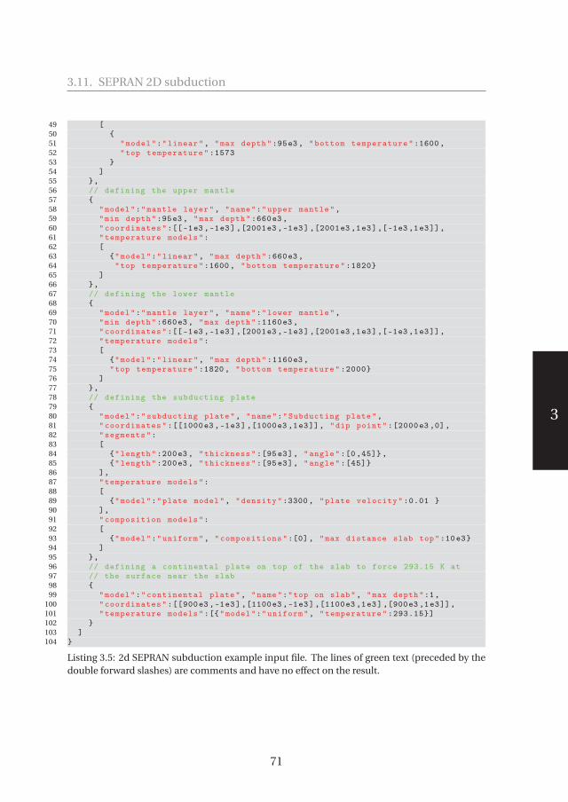
530578-L-sub01-bw-Fraters530578-L-sub01-bw-Fraters530578-L-sub01-bw-Fraters530578-L-sub01-bw-FratersProcessed on: 10-4-2019Processed on: 10-4-2019Processed on: 10-4-2019Processed on: 10-4-2019 PDF page: 81PDF page: 81PDF page: 81PDF page: 81
3
3.11. SEPRAN 2D subduction
49 [50 {51 "model":"linear", "max depth":95e3 , "bottom temperature":1600,52 "top temperature":157353 }54 ]55 },56 // defining the upper mantle57 {58 "model":"mantle layer", "name":"upper mantle",59 "min depth":95e3, "max depth":660e3,60 "coordinates":[[-1e3 ,-1e3] ,[2001e3 ,-1e3] ,[2001e3 ,1e3],[-1e3 ,1e3]],61 "temperature models":62 [63 {"model":"linear", "max depth":660e3,64 "top temperature":1600, "bottom temperature":1820}65 ]66 },67 // defining the lower mantle68 {69 "model":"mantle layer", "name":"lower mantle",70 "min depth":660e3, "max depth":1160e3 ,71 "coordinates":[[-1e3 ,-1e3] ,[2001e3 ,-1e3] ,[2001e3 ,1e3],[-1e3 ,1e3]],72 "temperature models":73 [74 {"model":"linear", "max depth":1160e3,75 "top temperature":1820, "bottom temperature":2000}76 ]77 },78 // defining the subducting plate79 {80 "model":"subducting plate", "name":"Subducting plate",81 "coordinates":[[1000e3 ,-1e3] ,[1000e3 ,1e3]], "dip point":[2000e3 ,0],82 "segments":83 [84 {"length":200e3 , "thickness":[95e3], "angle":[0 ,45]} ,85 {"length":200e3 , "thickness":[95e3], "angle":[45]}86 ],87 "temperature models":88 [89 {"model":"plate model", "density":3300, "plate velocity":0.01 }90 ],91 "composition models":92 [93 {"model":"uniform", "compositions":[0], "max distance slab top":10e3}94 ]95 },96 // defining a continental plate on top of the slab to force 293.15 K at97 // the surface near the slab98 {99 "model":"continental plate", "name":"top on slab", "max depth":1,
100 "coordinates":[[900e3 ,-1e3] ,[1100e3 ,-1e3] ,[1100e3 ,1e3],[900e3 ,1e3]],101 "temperature models":[{"model":"uniform", "temperature":293.15}]102 }103 ]104 }
Listing 3.5: 2d SEPRAN subduction example input file. The lines of green text (preceded by thedouble forward slashes) are comments and have no effect on the result.
71
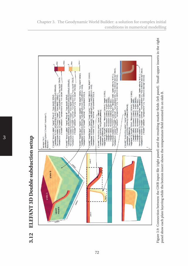
530578-L-sub01-bw-Fraters530578-L-sub01-bw-Fraters530578-L-sub01-bw-Fraters530578-L-sub01-bw-FratersProcessed on: 10-4-2019Processed on: 10-4-2019Processed on: 10-4-2019Processed on: 10-4-2019 PDF page: 82PDF page: 82PDF page: 82PDF page: 82
3
Chapter 3. The Geodynamic World Builder: a solution for complex initialconditions in numerical modelling
3.12
EL
EFA
NT
3DD
ou
ble
sub
du
ctio
nse
tup
Fig
ure
3.9:
Co
nn
ecti
on
bet
wee
nth
eG
WB
inp
ut
file
(rig
ht
pan
el)
and
the
resu
ltin
gm
arke
rfi
eld
s(l
eft
pan
el).
Smal
lup
per
inse
rts
inth
eri
ght
pan
elsh
owea
chp
late
laye
rin
gw
hile
the
bo
tto
min
sert
show
sth
ete
mp
erat
ure
fiel
dzo
om
edin
on
slab
B.
72

530578-L-sub01-bw-Fraters530578-L-sub01-bw-Fraters530578-L-sub01-bw-Fraters530578-L-sub01-bw-FratersProcessed on: 10-4-2019Processed on: 10-4-2019Processed on: 10-4-2019Processed on: 10-4-2019 PDF page: 83PDF page: 83PDF page: 83PDF page: 83
3
3.13. ASPECT 3d curved subduction
3.13 ASPECT 3d curved subduction1 {2 "version":"0.2",3 "potential mantle temperature":1500,4 "thermal expansion coefficient":2.0e-5,5 "maximum distance between coordinates":100000 ,6 "interpolation":"monotone spline",7 "surface temperature":293.15 ,8 "force surface temperature":true ,9 "coordinate system":{"model":"cartesian"},
10 "features":11 [12 // defining an oceanic plate for the North and South American plate13 {"model":"oceanic plate", "name":"NS American plate",14 "coordinates":[[1700e3 ,0] ,[1700e3 ,300e3] ,[1606e3 ,650e3],15 [1350e3 ,906e3] ,[1000e3 ,1000e3],[-1e3 ,1000 e3],16 [-1e3 ,1501 e3] ,[2501e3 ,1501 e3] ,[2501e3 ,-501e3],17 [-1e3 ,-501e3],[-1e3 ,-50e3] ,[2000e3 ,-50e3],18 [2000e3 ,0e3]],19 "temperature models":[{"model":"linear", "max depth":100e3}],20 "composition models":[{"model":"uniform", "compositions":[0],21 "max depth":30e3}]},2223 // Defining an oceanic plate for the Caribbean plate24 {"model":"oceanic plate", "name":"Caribbean plate",25 "coordinates":[[1700e3 ,300e3] ,[1689e3 ,422e3] ,[1658e3 ,539e3],26 [1606e3 ,650e3] ,[1536e3 ,749e3] ,[1450e3 ,836e3],27 [1350e3 ,906e3] ,[1239e3 ,958e3] ,[1122e3 ,989e3],28 [1000e3 ,1000e3],[650e3 ,1000e3],[-1e3 ,1000 e3],29 [-1e3 ,0e3] ,[1700e3 ,0e3]],30 "temperature models":[{"model":"linear", "max depth":100e3}],31 "composition models":[{"model":"uniform", "compositions":[1],32 "max depth":30e3}]},3334 // Defining a continental plate for the weak zone35 {"model":"continental plate", "name":"Carribean weak zone",36 "coordinates":[[-1e3 ,1000e3],[-1e3 ,750e3] ,[1536e3 ,749e3],37 [1450e3 ,836e3] ,[1350e3 ,906e3] ,[1239e3 ,958e3],38 [1122e3 ,989e3] ,[1000e3 ,1000e3] ,[650e3 ,1000 e3]],39 "temperature models":[{"model":"linear", "max depth":100e3}],40 "composition models":[{"model":"uniform", "compositions":[2],41 "max depth":30e3},42 {"model":"uniform", "compositions":[3],43 "min depth":30e3}]},4445 // Defining a mantle layer for the lower mantle46 {"model":"mantle layer", "name":"660", "min depth":660e3 ,47 "coordinates":[[-1e3 ,-500e3],[-501e3 ,2500e3] ,[2501e3 ,2500e3],48 [2501e3 ,-501e3]],49 "composition models":[{"model":"uniform", "compositions":[4]}]} ,5051 // Defining a subducting plate for the Lesser Antilles slab52 {"model":"subducting plate", "name":"Lesser Antilles slab",53 "coordinates":[[1700e3 ,0] ,[1700e3 ,300e3] ,[1606e3 ,650e3],54 [1350e3 ,906e3] ,[1000e3 ,1000e3] ,[650e3 ,1000 e3]],55 "dip point":[-1,-1],56 "min depth":0, "max depth":660e3,57 "segments":58 [59 {"length":300e3 , "thickness":[100e3], "angle":[0 ,50]},60 {"length":371e3 , "thickness":[100e3], "angle":[50]} ,61 {"length":275e3 , "thickness":[100e3], "angle":[50,0]},62 {"length":0e3, "thickness":[100 e3], "angle":[0]}63 ],
73

530578-L-sub01-bw-Fraters530578-L-sub01-bw-Fraters530578-L-sub01-bw-Fraters530578-L-sub01-bw-FratersProcessed on: 10-4-2019Processed on: 10-4-2019Processed on: 10-4-2019Processed on: 10-4-2019 PDF page: 84PDF page: 84PDF page: 84PDF page: 84
Chapter 3. The Geodynamic World Builder: a solution for complex initialconditions in numerical modelling
64 "sections":65 [66 {"coorindate":"0",67 "segments":68 [69 {"length":300e3 , "thickness":[100e3], "angle":[0,25]},70 {"length":371e3 , "thickness":[100e3], "angle":[50]} ,71 {"length":300e3 , "thickness":[100e3], "angle":[50 ,0]},72 {"length":50, "thickness":[100e3], "angle":[0]}73 ]74 },75 {"coorindate":"5",76 "segments":77 [78 {"length":300e3 , "thickness":[100e3], "angle":[0,25]},79 {"length":371e3 , "thickness":[100e3], "angle":[50]} ,80 {"length":50e3 , "thickness":[100e3], "angle":[50,0]} ,81 {"length":0, "thickness":[100e3], "angle":[0]}82 ]83 }84 ],85 "temperature models":86 [87 {"model":"plate model", "density":3300, "plate velocity":0.0144 ,88 "thermal conductivity":2.5, "thermal expansion coefficient":2e-5 }89 ],90 "composition models":91 [92 {"model":"uniform","compositions":[0], "min distance slab top":30e3}93 ]94 },9596 // Defining a continental plate for the weakzone between the Caribbean and97 // South America98 {"model":"continental plate","name":"South Weakzone",99 "coordinates":[[-1e3 ,0e3],[-1e3 ,-50e3] ,[2000e3 ,-50e3] ,[2000e3 ,0e3]],
100 "temperature models":[{"model":"linear", "max depth":100e3}],101 "composition models":102 [103 {"model":"uniform","compositions":[2], "max depth":30e3},104 {"model":"uniform", "compositions":[3], "min depth":30e3}]}105106 ]107 }
Listing 3.6: Input for the ASPECT example. The lines of green text (preceded by the doubleforward slashes) are comments and have no effect on the result.
74

530578-L-sub01-bw-Fraters530578-L-sub01-bw-Fraters530578-L-sub01-bw-Fraters530578-L-sub01-bw-FratersProcessed on: 10-4-2019Processed on: 10-4-2019Processed on: 10-4-2019Processed on: 10-4-2019 PDF page: 85PDF page: 85PDF page: 85PDF page: 85
4Assessing the geodynamics of strongly arcuatesubduction zones: the eastern Caribbeansubduction setting.
530578-L-sub01-bw-Fraters530578-L-sub01-bw-Fraters530578-L-sub01-bw-Fraters530578-L-sub01-bw-FratersProcessed on: 10-4-2019Processed on: 10-4-2019Processed on: 10-4-2019Processed on: 10-4-2019 PDF page: 86PDF page: 86PDF page: 86PDF page: 86
4
Chapter 4. Assessing the geodynamics of strongly arcuate subduction zones:the eastern Caribbean subduction setting.
4.1 SummaryIn this chapter I build on the accomplishments of Chapters 2 and 3 to create
a next step in numerical simulating the geodynamic evolution of natural sub-duction. The target natural system is that of strongly arcuate subduction whichis common on Earth. The eastern Caribbean Lesser-Antilles subduction systemis taken as the example system for 3D numerical simulation. I demonstrate forthis arcuate subduction system the geodynamical feasibility of westward di-rected trench-parallel slab transport through the mantle, i.e. slab dragging byNorth-American plate motion, of the northern slab segment while the easternslab is subducting at a mantle-stationary trench. The resistance of the ambientmantle against slab dragging as well as the lateral deformation of the arcuateslab create a complex 3-D stress field in the slab that deviates strongly fromthe classical view of slab-dip aligned orientation of slab stress. Slab draggingthus may reveal itself in the focal mechanisms of intermediate and deep earth-quakes. These characteristics of arcuate subduction are generic and may aswell apply to other arcuate subduction systems, such as Izu-Bonin-Marianasor the Aleutians-Alaska systems, where anomalous focal mechanisms of slabevents are observed. This chapter demonstrates the developed capabilities andcomputational feasibility towards assessing the 3D-complexity and geodynam-ics of natural subduction systems.
4.2 IntroductionNumerical three-dimensional (3D) thermo-mechanical modelling provides
a crucial means for investigating the geodynamic evolution of plate conver-gence involving lithosphere subduction. Particularly, subduction modelling fa-cilitates a way for creating quantitative links between crust-mantle processesand the various surface observations of plate convergence zones obtained fromgeological, seismological, or geodetic methods. Clearly, this requires the ca-pability of numerical simulation of natural subduction systems that are char-acterized by complex tectonic histories and 3D slab evolution. Advances inglobal mantle convection modelling have shown that plate motions and litho-sphere subduction can be sustained in a dynamically self-consistent way (e.g.
Assessing the geodynamics of strongly arcuate subduction zones: the eastern Caribbean sub-duction setting., M. Fraters, W. Spakman, C. Thieulot and D. van Hinsbergen, in preparation forpublication.
76

530578-L-sub01-bw-Fraters530578-L-sub01-bw-Fraters530578-L-sub01-bw-Fraters530578-L-sub01-bw-FratersProcessed on: 10-4-2019Processed on: 10-4-2019Processed on: 10-4-2019Processed on: 10-4-2019 PDF page: 87PDF page: 87PDF page: 87PDF page: 87
4
4.2. Introduction
Crameri and Tackley, 2015; Coltice and Shephard, 2017), but creating usefultectonic predictions for natural subduction is still difficult (Coltice and Shep-hard, 2017). When subduction modelling is restricted to a regional modellingdomain, it is easier to control governing plate motions through boundary con-ditions and impose initial model conditions derived from (paleo-)tectonic set-tings. Most investigations based on a regional model domain define an initial3D model in which plate boundaries are either parallel or perpendicular to therectangular boundaries (e.g. Stegman et al., 2006; Yamato et al., 2009; Burkettand Billen, 2010; Stegman et al., 2010a; van Hunen and Allen, 2011; Capitanioet al., 2011; Moresi et al., 2014; Schellart and Moresi, 2013; Duretz et al., 2014;Sternai et al., 2014; Magni et al., 2014; Pusok and Kaus, 2015; Capitanio et al.,2015; Kiraly et al., 2016; Sternai et al., 2016; Schellart, 2017; Pusok et al., 2018;Chertova et al., 2018; Gülcher et al., 2019). In this setup, subduction developsfrom an initially straight trench with trench-perpendicular plate convergenceand is controlled by the trench-perpendicular forcing of slab pull and conver-gent plate motions. Much less studies have attempted to simulate natural sub-duction by implementing constraints from the first-order inferences of, e.g.,governing trench-oblique plate motions, lithosphere structure and trench ge-ometry, or from plate-tectonic reconstructions (e.g. Billen and Gurnis, 2003; Liuand Stegman, 2011; Jadamec and Billen, 2010; Jadamec et al., 2013; Malatestaet al., 2013; Chertova et al., 2014b, 2018; Hu and Liu, 2016). This class of subduc-tion modelling, however, entails resolving the practical difficulty of construct-ing geometrically complex 3D initial models for the paleogeographic setting ofincipient subduction or for an advanced stage of subduction evolution.
The research we report here is in the realm of the latter modelling approachand assesses the geodynamics of natural subduction zones that are charac-terized by strongly trench-oblique plate convergence. We focus our investi-gation on the geodynamical processes involved in strongly arcuate subduc-tion. Prominent examples of such subduction systems are the major Aleutian-Alaska, Izu-Bonin-Marianas, or Andaman-Sumatra subduction zones. Theseare characterized by large absolute plate motions of the subducting plate atthe trench, ranging between 70-110 mm/yr, and by directions of plate con-vergence that vary from near trench-perpendicular (at the Alaska, Marianas,and east-Sumatra trenches, respectively) to strongly trench-oblique with de-partures from trench-perpendicular convergence by 60° to even 90° (e.g. Fig.S4 of Doubrovine et al. (2012)). Much smaller arcuate subduction systems withsignificant trench-parallel components of subducting plate motion occur in theMediterranean region. These systems involve low absolute plate motion of the
77

530578-L-sub01-bw-Fraters530578-L-sub01-bw-Fraters530578-L-sub01-bw-Fraters530578-L-sub01-bw-FratersProcessed on: 10-4-2019Processed on: 10-4-2019Processed on: 10-4-2019Processed on: 10-4-2019 PDF page: 88PDF page: 88PDF page: 88PDF page: 88
4
Chapter 4. Assessing the geodynamics of strongly arcuate subduction zones:the eastern Caribbean subduction setting.
subducting African plate to the NNE that varies between ~8 mm/yr for the east-dipping Gibraltar subduction in the western Mediterranean, to ~10 mm/yr forthe northwest-dipping Calabria subduction of the Central Mediterranean, to~12 mm/yr for NNE-dipping Aegean subduction of the Eastern Mediterranean.
The Lesser Antilles subduction of the eastern Caribbean region (Fig. 4.1A) isa strongly arcuate subduction system that is similar in geometry with the threemajor systems while it involves relatively small absolute motion of the subduct-ing North and South American plates of at present ~20 mm/yr in westward di-rection. The plate-tectonic setting, geometry, and evolution of the Lesser An-tilles subduction system are used here as a guide for our assessment of thegeodynamics of arcuate subduction that involves low subducting-plate mo-tion. Because it is unknown how arcuate subduction initializes, we focus ourresearch here on taking a more advanced evolution stage of established arcu-ate subduction as the starting point for modeling for which we create an ini-tial 3D model using our recently developed ’Geodynamic World Builder’ (GWB;version 0.1.0) (Fraters et al. 2019b, submitted to Solid Earth; Chapter 3). TheGWB is a versatile open-source software tool for the relatively easy constructionof geometrically intricate initial temperature-composition models for geody-namic modelling. It allows construction of complex 3D subduction geometriesas a starting point for generic modelling, for testing plate-tectonic evolutionscenarios, for investigating the evolution of natural subduction, or for the in-stantaneous dynamics of present-day subduction.
We employ the GWB to construct an approximation of the 3D geometry ofthe 3D Lesser Antilles subduction zone at ~10 Ma including overriding and sub-ducting plates. Our aim is two-fold. First, we experiment with various rheol-ogy and temperature settings of the initial model enabling local exploration ofthe model space for the style of subduction evolution. Particularly, we aim toobtain parameter settings for crust-mantle rheology such that a more or lessmantle-stationary eastern Lesser Antilles trench is obtained as is suggested byplate reconstructions in several mantle reference frames (Müller et al., 1999;Boschman et al., 2014). Second, we investigate the hypothesis that, while theeastern Lesser Antilles slab is mantle-stationary, the northern limb of the LesserAntilles subduction is subject to strong near trench-parallel lateral transport ofthe slab by the absolute motion of the North American plate, which is an ex-ample of slab dragging (Spakman et al., 2018). Our main purpose is to investi-gate how such an arcuate slab system develops from the interplay between 1)slab dragging forced by the absolute motion of the North and South Americanplates, 2) the almost not moving overriding Caribbean plate, 3) the vertically-
78
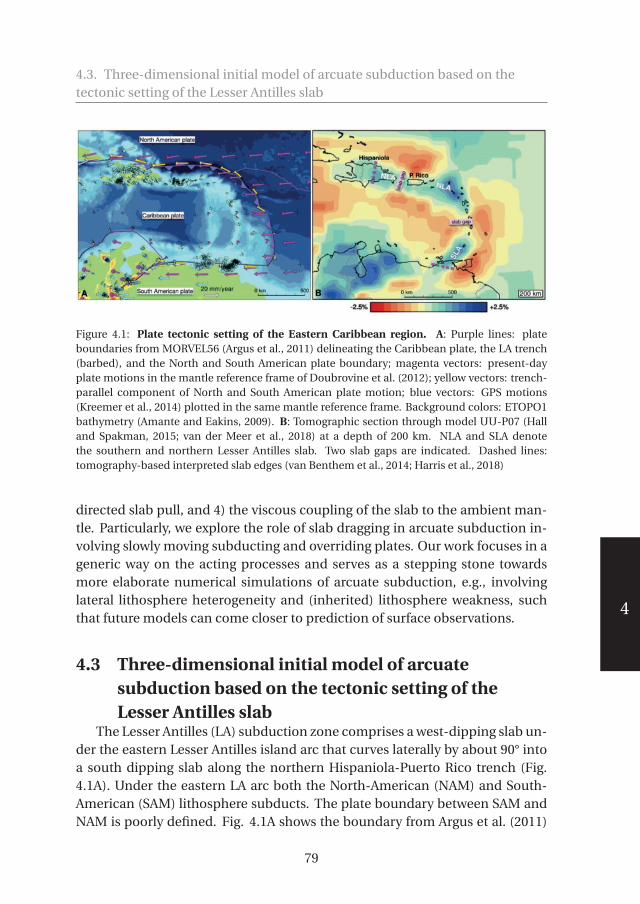
530578-L-sub01-bw-Fraters530578-L-sub01-bw-Fraters530578-L-sub01-bw-Fraters530578-L-sub01-bw-FratersProcessed on: 10-4-2019Processed on: 10-4-2019Processed on: 10-4-2019Processed on: 10-4-2019 PDF page: 89PDF page: 89PDF page: 89PDF page: 89
4
4.3. Three-dimensional initial model of arcuate subduction based on thetectonic setting of the Lesser Antilles slab
Figure 4.1: Plate tectonic setting of the Eastern Caribbean region. A: Purple lines: plateboundaries from MORVEL56 (Argus et al., 2011) delineating the Caribbean plate, the LA trench(barbed), and the North and South American plate boundary; magenta vectors: present-dayplate motions in the mantle reference frame of Doubrovine et al. (2012); yellow vectors: trench-parallel component of North and South American plate motion; blue vectors: GPS motions(Kreemer et al., 2014) plotted in the same mantle reference frame. Background colors: ETOPO1bathymetry (Amante and Eakins, 2009). B: Tomographic section through model UU-P07 (Halland Spakman, 2015; van der Meer et al., 2018) at a depth of 200 km. NLA and SLA denotethe southern and northern Lesser Antilles slab. Two slab gaps are indicated. Dashed lines:tomography-based interpreted slab edges (van Benthem et al., 2014; Harris et al., 2018)
directed slab pull, and 4) the viscous coupling of the slab to the ambient man-tle. Particularly, we explore the role of slab dragging in arcuate subduction in-volving slowly moving subducting and overriding plates. Our work focuses in ageneric way on the acting processes and serves as a stepping stone towardsmore elaborate numerical simulations of arcuate subduction, e.g., involvinglateral lithosphere heterogeneity and (inherited) lithosphere weakness, suchthat future models can come closer to prediction of surface observations.
4.3 Three-dimensional initial model of arcuatesubduction based on the tectonic setting of theLesser Antilles slab
The Lesser Antilles (LA) subduction zone comprises a west-dipping slab un-der the eastern Lesser Antilles island arc that curves laterally by about 90° intoa south dipping slab along the northern Hispaniola-Puerto Rico trench (Fig.4.1A). Under the eastern LA arc both the North-American (NAM) and South-American (SAM) lithosphere subducts. The plate boundary between SAM andNAM is poorly defined. Fig. 4.1A shows the boundary from Argus et al. (2011)
79

530578-L-sub01-bw-Fraters530578-L-sub01-bw-Fraters530578-L-sub01-bw-Fraters530578-L-sub01-bw-FratersProcessed on: 10-4-2019Processed on: 10-4-2019Processed on: 10-4-2019Processed on: 10-4-2019 PDF page: 90PDF page: 90PDF page: 90PDF page: 90
4
Chapter 4. Assessing the geodynamics of strongly arcuate subduction zones:the eastern Caribbean subduction setting.
while interpretations of seismic tomography suggest it coincides with a gap inthe slab that is imaged to depths of 200-300 km separating the southern LesserAntilles slab (SLA) from the northern Lesser Antilles (NLA) slab (Fig. 4.1B; vanBenthem et al., 2013; Harris et al., 2018). Another slab gap between Hispaniolaand Puerto Rico (Fig. 4.1B) was proposed by Harris et al. (2018), while Meighanet al. (2013) suggest vertical slab segmentation to the east of Puerto Rico. Thearcuate slab geometry is well delineated by slab seismicity to depths of ~200km (Harris et al., 2018) and in the upper mantle by seismic tomography vanBenthem et al. (2013); Harris et al. (2018).
In a plate motion frame relative to the Caribbean plate, the NAM plateconverges at present highly oblique at an angle of ~20° with the strike of thenorthern trench. This suggests a component of westward trench-parallel mo-tion of the NLA slab with respect to the Caribbean plate (van Benthem et al.,2014). Investigating actual slab motion through the mantle requires a man-tle frame of reference (e.g. Doubrovine et al. (2012)) to define the absoluteplate motion (APM) of the NAM and SAM subducting plates and that of theoverriding Caribbean plate. Along the eastern trench, the APM of the NAMand SAM plates is at present largely trench-perpendicular in the south and in-creasingly trench-oblique when going to the north, while the NAM plate movesnear trench-parallel along the northern trench (Fig. 4.1A). The Caribbean plateshows at present little motion in the mantle frame (Fig. 4.1A) while the smallGPS motions of the LA islands above the eastern LA slab imply that the east-ern LA trench may also be about mantle-stationary. This plate-tectonic settingin the mantle reference frame suggests that the NLA slab is at present beingtransported almost trench-parallel through the upper mantle by the APM ofthe NAM plate whereas the eastern LA slab is subducting at a mantle-stationarytrench.
The trench-parallel slab motion is an example of slab dragging, i.e., ’the pro-cess of lateral slab transport through the mantle that is forced by the absolutesurface motion of the subducting plate’ (Spakman et al., 2018). Slab draggingat a rate of 6-7 mm/yr has recently been documented for the Gibraltar slab ofthe western Mediterranean (Spakman et al. 2018), and at a trench-parallel rateof about 30 mm/yr for the Tonga-Kermadec slab (van de Lagemaat et al., 2018).The actual occurrence and effects of slab dragging on slab deformation duringarcuate subduction are here important targets of investigation.
We employ the GWB to reconstruct the 3D subduction zone geometry forsetting up an initial geometrical model that simulates 3D slab morphology at10 Ma and which implements overriding and subducting plates. By doing so
80

530578-L-sub01-bw-Fraters530578-L-sub01-bw-Fraters530578-L-sub01-bw-Fraters530578-L-sub01-bw-FratersProcessed on: 10-4-2019Processed on: 10-4-2019Processed on: 10-4-2019Processed on: 10-4-2019 PDF page: 91PDF page: 91PDF page: 91PDF page: 91
4
4.3. Three-dimensional initial model of arcuate subduction based on thetectonic setting of the Lesser Antilles slab
we avoid defining the poorly constrained paleogeographic and plate tectonicsetting of subduction initiation in the Paleogene(e.g. Pindell and Kennan, 2009;Boschman et al., 2014). Another advantage is that we can reduce the compu-tation time for such complex subduction models. The Caribbean plate hasbeen more or less mantle-stationary since the Paleogene (Müller et al., 1999;Boschman et al., 2014). Assuming that the eastern LA trench has also beenmantle-stationary, the simplest reconstruction for 10 Myr ago requires shiftingthe NAM plate, and thus the northern slab edge, to the east. Given the largeuncertainty of absolute plate motions (Doubrovine et al., 2012), we assumea mantle-stationary Caribbean plate and use the more accurate relative platemotion between the Caribbean and NAM for NAM of ~15 mm/yr during thepast 10 Myr (Boschman et al., 2014). We adopt this value for the west-directedAPM of both NAM and SAM. This choice keeps our approximation of the LesserAntilles subduction close enough to the actual system while our generic mod-elling can focus on assessing the dynamics of arcuate subduction at low APM ofthe subducting plate and close to the African APM involved in arcuate Mediter-ranean subduction systems.
Effectively, for the construction of the slab geometry at 10 Ma we estimatethe first-order geometrical characteristics (dip, length, curvature) of the tomo-graphically imaged slab of Harris et al. (2018) and remove 150 km from thewestern part of the slab. This leads to the slab geometry of Fig. 4.2. Impor-tantly, the 150 km eastward shift of the slab at 10 Ma is just an assumption andprovides a starting geometry. Modelling forward in time, the slab evolution mayshow if the resulting slab geometry at 0 Ma conforms to the tomographic ob-servation. For instance, this would provide a primary test of the hypothesis thatthe NLA slab is being entirely dragged westward by the APM of the NAM plate,instead of only partially, or not significantly.
A Cartesian model box is adopted with X-Y-Z dimensions of 2500 km × 2000km × 800 km. The initial model is built from six different GWB-features whichare assigned GWB-compositions for identification. The background tempera-ture is defined by the adiabatic geotherm θS exp(αg d/Cp ), where θS is the po-tential temperature of the mantle (1500 K), α is the thermal expansion coeffi-cient (2×10⁻⁵ K−1), g is the gravitational acceleration (m/s2), Cp is the specificheat (1250 J· kg−1 K−1) and d is the depth. When no composition label is de-fined, the background composition is assumed, i.e. the mantle. This holds forinstance for the lithospheric mantle of the tectonic plates. The initial modelconsists of the following parts:
• The North and South American plate, which are combined here into one
81

530578-L-sub01-bw-Fraters530578-L-sub01-bw-Fraters530578-L-sub01-bw-Fraters530578-L-sub01-bw-FratersProcessed on: 10-4-2019Processed on: 10-4-2019Processed on: 10-4-2019Processed on: 10-4-2019 PDF page: 92PDF page: 92PDF page: 92PDF page: 92
4
Chapter 4. Assessing the geodynamics of strongly arcuate subduction zones:the eastern Caribbean subduction setting.
Figure 4.2: Initial subduction model geometry and velocity boundary conditions. A: Regionscomposing the crust. The thickness of the Caribbean, NAM and SAM crust is 30 km and itsrheology is tunable separately from the lithospheric mantle. Weakness zones of tunable rhe-ology provide visco-plastic decoupling between the Caribbean and NAM and SAM plates. Thelithospheric mantle is configured as part of the mantle and shown in B. The NAM and SAM litho-sphere obtain uniform west pointing plate velocity which is imposed on the vertical model edgesand across the lithosphere thickness of 100 km. The top of the model is a dynamic free surface.B: Temperature view of the 3D lithosphere starting model. Temperature in the lithosphere in-creases linearly. In the slab, a temperature field is shown computed from the analytical solutionprovided by McKenzie (1970). Slabs with different initial temperature are used in experiments.The three transparent zones plotted on the slab and labeled w(est),c(entral), and e(ast), denotelocations of a priori inserted vertical slab weakness zones used for experimenting.
82

530578-L-sub01-bw-Fraters530578-L-sub01-bw-Fraters530578-L-sub01-bw-Fraters530578-L-sub01-bw-FratersProcessed on: 10-4-2019Processed on: 10-4-2019Processed on: 10-4-2019Processed on: 10-4-2019 PDF page: 93PDF page: 93PDF page: 93PDF page: 93
4
4.3. Three-dimensional initial model of arcuate subduction based on thetectonic setting of the Lesser Antilles slab
plate, North-South American (NSAM) plate, is given a thickness of 100km and a linear temperature profile from the surface temperature (293K) to the adiabatic temperature at the depth of 100 km. The crustal layeris represented by compositional layer 0 and is 30 km in thickness.
• The Caribbean plate only differs from the North-South American plate byits compositional label 1 for the crust.
• The LA trench together with the subducting slab is the next GWB-feature.The trench is defined by 12 trench points, interpolated by a monotonespline, that effectively describe 3 main lateral trench sectors: the east-ern trench, the curved trench, and the more or less EW-striking northerntrench (Fig. 4.2A). In each trench point the slab is parameterized by 4four depth segments along a vertical section. The first 3 segments obtainthe same dip variation while the 4th, deepest segment, varies in geomet-rical properties along the trench from SE to NW. The thickness of all slabsegments is equal to the thickness of the subducting North-South Amer-ican plate, i.e. 100 km. Laterally, the geometrical properties are linearlyinterpolated between the 12 vertical trench-slices. The first slab segmenthas a length of 150 km and starting-dip angle of 0°, i.e. parallel with thesurface, which increases linearly with depth to 25°. The second segment,also of 150 km, starts with a dip angle of 25° which linearly increases alongthe segment to 50°. The third segment has a length of 171 km and dipsuniformly at 50°. The last segment is of variable length but the dip anglein each trench slice changes linearly from 50° to 0°. In the eastern mainslab sector, from the SE slab edge to the beginning of the slab bend, thelength of the fourth depth segment varies from 300 km to 275 km. In thebend-sector, the length is 275 km and after the bend, i.e. the northernslab sector, the length varies from 275 to 50 km. The temperature in theplate is defined by the McKenzie (1970) temperature model and the top30 km of the slab has compositional label 0. The southern sector has thelargest slab length of 875 km and reaches the depth of 660 km at the tran-sition to the lower mantle. In 10 Myr of subduction evolution the lengthwould increase to ~1025 km which underestimates the ~1100 km of sub-duction since ~45 Ma (Boschman et al., 2014). This is done to avoid toostrong coupling between slab and lower mantle in all numerical models.Effects of possible deep upper-mantle anchoring of the slab (e.g. Uyedaand Kanamori, 1979; Heuret and Lallemand, 2005) will be tested in ex-periments with an increased viscosity in the deeper upper mantle.
83
530578-L-sub01-bw-Fraters530578-L-sub01-bw-Fraters530578-L-sub01-bw-Fraters530578-L-sub01-bw-FratersProcessed on: 10-4-2019Processed on: 10-4-2019Processed on: 10-4-2019Processed on: 10-4-2019 PDF page: 94PDF page: 94PDF page: 94PDF page: 94
4
Chapter 4. Assessing the geodynamics of strongly arcuate subduction zones:the eastern Caribbean subduction setting.
• To the west of the northern slab edge under Hispaniola, a 100 kmthick and 250 km wide lithosphere plate is defined with the same lin-ear geotherm as in the adjacent plates. The zone is extended to the eastwhere it partly replaces the Caribbean plate (top green zone of Fig. 4.2A).To west of the slab edge, this continental zone will serve as a weak zonedecoupling the North American and Caribbean plates whereas it definesa weak upper plate above the NLA slab. The continental segment is givena separate composition label 2 for the crust and composition label 3 forthe deeper lithosphere, which enables tuning the lithosphere rheologyseparately from the adjacent plates.
• A similar lithospheric weak zone of thickness 100 km and width 50 kmdecouples the South American plate from the Caribbean plate and theslab. Composition labels are the same as for the northern weak zone.
• The lower mantle below 660 km is separately defined with compositionlabel 4.
To test the effects of lateral rheological slab heterogeneity, e.g. subductedinherited weak zones, vertical segments of slab have been assigned a separatecompositional label 2 for the crustal part and label 3 for the lithospheric partof the slab, such that the rheology can be assigned to be weaker then the sur-rounding slab. Weak zones can be placed in three locations (Fig. 4.2B).
Depending on the compositional label, all model features can be assignedspecific material rheology. Rheology and slab temperature will be defined ineach numerical experiment leading to a complete definition of the initial con-ditions.
The details of how the model is setup through the GWB can be found inappendix 4.7.
4.4 Model setup4.4.1 Numerical model setup
Modelling the dynamic evolution of subduction requires numerically solv-ing the governing equations of continuum mechanics for which modern, opensource, parallel geodynamics codes are available, such as pTatin (May et al.,2015), LaMem (Kaus et al., 2016), Citcom(S) Zhong et al. (2000), Underworld 2(Mansour et al., 2019), or ASPECT (Kronbichler et al., 2012; Heister et al., 2017).In this thesis we use version 2.1.0-pre of ASPECT with some unmerged but pro-posed changed at the time of writing. The most significant changes are three
84

530578-L-sub01-bw-Fraters530578-L-sub01-bw-Fraters530578-L-sub01-bw-Fraters530578-L-sub01-bw-FratersProcessed on: 10-4-2019Processed on: 10-4-2019Processed on: 10-4-2019Processed on: 10-4-2019 PDF page: 95PDF page: 95PDF page: 95PDF page: 95
4
4.4. Model setup
added plugins. The first plugin is a boundary temperature model which pre-scribes the initial temperature to all boundaries, except for the surface, where afixed temperature is set. Secondly a mesh refinement model which allows to setminimum and maximum refinement levels between a pre-set minimum andmaximum temperature. Thirdly, a postprocessor which computes the maxi-mum shear stress. This is computed by first computing the eigenvalues andeigenvectors of the stress tensor. The direction of the maximum shear is thencomputed by subtracting the smallest eigenvector from the largest eigenvector.The magnitude is computed by subtracting smallest eigenvalue by the largesteigenvalue and dividing it by two. The exact setup can be found in appendix4.8, which shows the reference ASPECT input file.
Governing equationsThe mass, momentum and energy conservation equations are those of a
fluid under the Boussinesq approximation (Schubert et al., 2001):
−∇· (2ηε(u))+∇p = ρg in Ω, (4.1)
∇·u = 0 in Ω, (4.2)
ρ0Cp
(∂T
∂t+u ·∇T
)−∇·k∇T = ρH in Ω, (4.3)
∂ci
∂t+u ·∇ci = qi in Ω, i = 1. . .C (4.4)
where u is the velocity, p the pressure and T the temperature. The set of ad-vected quantities ci are called compositional fields and are used to track mate-rials. The coefficient are as follows: η is the viscosity, ρ the density, g the gravityvector and ε(·) denotes the (deviatoric) symmetric gradient operator definedby ε(v) = 1
2 (∇v+∇vT), Cp is the specific heat, k the thermal conductivity and His the internal heat production. Note that all coefficients that appear in theseequations can depend on the pressure, temperature, chemical composition,and the strain rate, thereby making these equations potentially nonlinear.
In our modelling we have used the default Finite Element type of ASPECT,i.e. the Q2 ×Q1 element (Gresho and Sani, 2000). Details of the Finite Elementdiscretization of the above equations can be found in Chapter 2 as well as inKronbichler et al. (2012); Heister et al. (2017). All simulations were performedwith the stabilized Newton solver, as described in Chapter 2, and run in par-allel on 480 threads on five nodes made from AMD EPYC 7451 24-Core Pro-cessors. Depending on the chosen set of rheological parameters simulationstook between 3 and 6 days to simulate 10 million years. In the reference model,
85
530578-L-sub01-bw-Fraters530578-L-sub01-bw-Fraters530578-L-sub01-bw-Fraters530578-L-sub01-bw-FratersProcessed on: 10-4-2019Processed on: 10-4-2019Processed on: 10-4-2019Processed on: 10-4-2019 PDF page: 96PDF page: 96PDF page: 96PDF page: 96
4
Chapter 4. Assessing the geodynamics of strongly arcuate subduction zones:the eastern Caribbean subduction setting.
the number of elements varies through time between 560000 and 660000. Thenumber of Stokes degrees of freedom (dofs) vary between 15 and 18 million, thenumber of temperature dofs between 4.7 and 5.7 million and the total numberof composition dofs between 23 and 28 million over a total simulation time of20 million years.
4.4.2 Boundary conditionsThe 6 geometrical boundaries of the regional model box comprise ten dif-
ferent boundary domains for defining boundary conditions: a top and bottomboundary, four side boundaries above 100 km depth and four side boundariesbelow 100 km depths. The top boundary is a (stabilized) free surface (Rose et al.,2017; Kaus et al., 2010; Quinquis et al., 2011). On the bottom boundary a zerovelocity boundary condition (no-slip) is defined. The four bottom side bound-aries are open boundaries (Chertova et al., 2012) which were implemented inASPECT by Anne Glerum (Glerum et al., 2018). The eastern and western topside boundaries are assigned velocity boundary condition (Dirichlet type) of1.5 cm/yr (or 3.0 cm/yr in some experiments), uniformly pointing to the westin most of the domain. At the Caribbean plate the boundary velocity is set tozero, and in the weak zones the velocity linearly increases from zero at the sideof the Caribbean plate to 1.5 (or 3.0 cm/yr) in the NSAM plate. To compensatefor the lower outflow in the southern weak zone, there is slightly less inflowon the south-east of the model. The north and south boundaries have for the xand y component an open boundary condition, where the z component is fixedto zero velocity. Temperature boundary conditions are set along the sides andbottom according to the initial model. For details on the boundary conditions,see the ASPECT input file in section 4.8.
4.4.3 Rheological modelFor the rheology we use a composite viscosity model consisting of three ef-
fective viscosities computed for each composition i as follows:
• the effective dislocation creep viscosity:
ηdsli = 1
2A− 1
ni εi
1−nini exp
(E∗i +PV ∗
i
ni RT
)• the effective diffusion creep viscosity:
ηdffi = 1
2A−1d
mini exp
(E∗i +PV ∗
i
RT
)86

530578-L-sub01-bw-Fraters530578-L-sub01-bw-Fraters530578-L-sub01-bw-Fraters530578-L-sub01-bw-FratersProcessed on: 10-4-2019Processed on: 10-4-2019Processed on: 10-4-2019Processed on: 10-4-2019 PDF page: 97PDF page: 97PDF page: 97PDF page: 97
4
4.4. Model setup
• the effective plastic viscosity:
ηpli = p sinφi + ci cosφi�
3(3+ sinφi ) 2εi
which is a commonly used formulation in geodynamics, based on theDrucker-Prager yield criterion (Glerum et al., 2018; Spiegelman et al.,2016).
In these equations εi is the square root of the second invariant of the strainrate tensor, R is the gas constant, and P and T are the pressure and temper-ature. The full pressure is used in these equations, including in the plasticity,and not the lithostatic pressure as in Chertova et al. (2014a). Although using thefull pressure in the plasticity has been shown to be potentially problematic forthe solvers (Spiegelman et al., 2016), we obtained convergence to a nonlinearnormalized tolerance level of 10−6 within the first few time steps.
We make use of the pre-existing "visco plastic" material model of ASPECT,which first separately computes the three viscosities and then combines themas follows:
1. a composite viscous viscosity is first computed through
ηvisc =(
1
ηdffi
+ 1
ηdsli
)−1
2. if the associated viscous stress 2ηvi sc εi exceeds the plastic yield strengththen the plastic viscosity ηpl is used instead of ηvi sc ;
3. if more than one compositional field is present at a given point, viscosi-ties are averaged with a harmonic scheme (Schmeling et al. (2008)).
Finally, in order to avoid too poorly conditioned matrices, the resulting ef-fective viscosities ηeff are bounded such that:
ηmin ≤ ηeff ≤ ηmax (4.5)
where ηmin and ηmax are user-chosen parameters that typically define a rangeof 5-6 orders of magnitude.
There are 5 materials in our model, each associated with density, thermaland rheological parameters. The rheological parameters of these materials arelisted in Table 4.1.
87
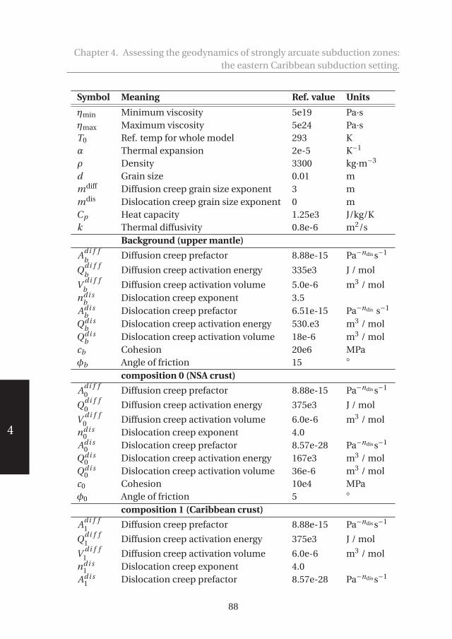
530578-L-sub01-bw-Fraters530578-L-sub01-bw-Fraters530578-L-sub01-bw-Fraters530578-L-sub01-bw-FratersProcessed on: 10-4-2019Processed on: 10-4-2019Processed on: 10-4-2019Processed on: 10-4-2019 PDF page: 98PDF page: 98PDF page: 98PDF page: 98
4
Chapter 4. Assessing the geodynamics of strongly arcuate subduction zones:the eastern Caribbean subduction setting.
Symbol Meaning Ref. value Units
ηmin Minimum viscosity 5e19 Pa·sηmax Maximum viscosity 5e24 Pa·sT0 Ref. temp for whole model 293 Kα Thermal expansion 2e-5 K−1
ρ Density 3300 kg·m−3
d Grain size 0.01 mmdiff Diffusion creep grain size exponent 3 mmdis Dislocation creep grain size exponent 0 mCp Heat capacity 1.25e3 J/kg/Kk Thermal diffusivity 0.8e-6 m2/s
Background (upper mantle)
Adi f fb Diffusion creep prefactor 8.88e-15 Pa−ndis s−1
Qdi f fb Diffusion creep activation energy 335e3 J / mol
V di f fb Diffusion creep activation volume 5.0e-6 m3 / mol
ndi sb Dislocation creep exponent 3.5
Adi sb Dislocation creep prefactor 6.51e-15 Pa−ndis s−1
Qdi sb Dislocation creep activation energy 530.e3 m3 / mol
Qdi sb Dislocation creep activation volume 18e-6 m3 / mol
cb Cohesion 20e6 MPaφb Angle of friction 15 ◦
composition 0 (NSA crust)
Adi f f0 Diffusion creep prefactor 8.88e-15 Pa−ndis s−1
Qdi f f0 Diffusion creep activation energy 375e3 J / mol
V di f f0 Diffusion creep activation volume 6.0e-6 m3 / mol
ndi s0 Dislocation creep exponent 4.0
Adi s0 Dislocation creep prefactor 8.57e-28 Pa−ndis s−1
Qdi s0 Dislocation creep activation energy 167e3 m3 / mol
Qdi s0 Dislocation creep activation volume 36e-6 m3 / mol
c0 Cohesion 10e4 MPaφ0 Angle of friction 5 ◦
composition 1 (Caribbean crust)
Adi f f1 Diffusion creep prefactor 8.88e-15 Pa−ndis s−1
Qdi f f1 Diffusion creep activation energy 375e3 J / mol
V di f f1 Diffusion creep activation volume 6.0e-6 m3 / mol
ndi s1 Dislocation creep exponent 4.0
Adi s1 Dislocation creep prefactor 8.57e-28 Pa−ndis s−1
88

530578-L-sub01-bw-Fraters530578-L-sub01-bw-Fraters530578-L-sub01-bw-Fraters530578-L-sub01-bw-FratersProcessed on: 10-4-2019Processed on: 10-4-2019Processed on: 10-4-2019Processed on: 10-4-2019 PDF page: 99PDF page: 99PDF page: 99PDF page: 99
4
4.4. Model setup
Qdi s1 Dislocation creep activation energy 223e3 m3 / mol
Qdi s1 Dislocation creep activation volume 18e-6 m3 / mol
c1 Cohesion 10e6 MPaφ1 Angle of friction 10 ◦
composition 2 (weakzone crust)
Adi f f2 Diffusion creep prefactor 8.88e-15 Pa−ndis s−1
Qdi f f2 Diffusion creep activation energy 375e3 J / mol
V di f f2 Diffusion creep activation volume 6.0e-6 m3 / mol
ndi s2 Dislocation creep exponent 4.0
Adi s2 Dislocation creep prefactor 8.57e-28 Pa−ndis s−1
Qdi s2 Dislocation creep activation energy 167e3 m3 / mol
Qdi s2 Dislocation creep activation volume 18e-6 m3 / mol
c2 Cohesion 10e4 MPaφ2 Angle of friction 5 ◦
composition 3 (weakzone lithosphere)
Adi f f3 Diffusion creep prefactor 8.88e-15 Pa−ndis s−1
Qdi f f3 Diffusion creep activation energy 335e3 J / mol
V di f f3 Diffusion creep activation volume 6.0e-6 m3 / mol
ndi s3 Dislocation creep exponent 3.8
Adi s3 Dislocation creep prefactor 6.51e-15 Pa−ndis s−1
Qdi s3 Dislocation creep activation energy 440e3 m3 / mol
Qdi s3 Dislocation creep activation volume 18e-6 m3 / mol
c3 Cohesion 10e6 MPaφ3 Angle of friction 10 ◦
composition 4 (lower mantle)
Adi f f4 Diffusion creep prefactor 8.88e-15 Pa−ndis s−1
Qdi f f4 Diffusion creep activation energy 335e3 J / mol
V di f f4 Diffusion creep activation volume 6.0e-6 m3 / mol
ndi s4 Dislocation creep exponent 3.5
Adi s4 Dislocation creep prefactor 6.51e-15 Pa−ndis s−1
Qdi s4 Dislocation creep activation energy 530e3 m3 / mol
Qdi s4 Dislocation creep activation volume 18e-6 m3 / mol
c4 Cohesion 20e6 MPaφ4 Angle of friction 15 ◦
Table 4.1: List of Parameters for the reference model
89

530578-L-sub01-bw-Fraters530578-L-sub01-bw-Fraters530578-L-sub01-bw-Fraters530578-L-sub01-bw-FratersProcessed on: 10-4-2019Processed on: 10-4-2019Processed on: 10-4-2019Processed on: 10-4-2019 PDF page: 100PDF page: 100PDF page: 100PDF page: 100
4
Chapter 4. Assessing the geodynamics of strongly arcuate subduction zones:the eastern Caribbean subduction setting.
4.5 ExperimentsMany dozens of experiments were needed in search for acceptable rheolog-
ical settings. The initial model, although geometrically constrained by present-day mantle structure, plate motions and tectonic evolution, requires definitionof the initial rheology and temperature field. Particularly, we searched for man-tle rheology, within acceptable bounds, that would allow for a smooth continu-ation of subduction from the starting model avoiding complications such as,e.g., immediate detachment/necking of the slab, or other strong changes inslab morphology. Such ’sudden’ slab morphology variation would be an abruptchange from the gradual 30-35 Myr of slab evolution leading to the arcuateslab geometry we reconstructed for 10 Ma. Moreover, strong slab morphologychanges would also not be consistent with the present-day tomographic obser-vation which provides a strong constraint on our modelling. Also, many modelexperiments were conducted to find rheology settings that would create a moreor less mantle-stationary trench during 10 Myr of model evolution while still al-lowing for gradual slab morphology change in the upper mantle depending on(weak, intermediate, or strong) rheology of the deeper upper mantle.
We present a selection of models that assess the geodynamics of arcuatesubduction in various ways. We have adopted one model as the referencemodel, relative to which we will discuss the effects of variations in initial modelgeometry, plate velocities, and model rheology. The selection of models pre-sented here is based on the parameters which were most influential on modelevolution, particularly, for obtaining ongoing subduction at a more or less sta-tionary eastern LA trench in this setup of arcuate subduction.
The variations of the reference model concern using a weaker and strongercrust of the NSAM plate and of plate boundary weak zones, variation of themantle strength and of slab temperature, addition of compositional weak zonesin the slab and the effect of doubling the NSAM plate velocity. The full set ofdiscussed models is shown in table 4.2.
4.5.1 The reference modelThe starting geometry of the reference model is discussed in section 4.2. Af-
ter ample experimentation we arrived at the rheology and temperature settings,as described in table 4.1. Starting point for the rheological parameters comefrom Gleason and Tullis (1995); Karato (2008); Hirth and Kohlstedt (2003). Thereference model rheology is tuned to provide a more or less stationary trench.Figure 4.3 shows the reference model after 10 Myr of simulation, presentedwith similar view angles as in figure 4.2 giving an overall impression of the flow
90

530578-L-sub01-bw-Fraters530578-L-sub01-bw-Fraters530578-L-sub01-bw-Fraters530578-L-sub01-bw-FratersProcessed on: 10-4-2019Processed on: 10-4-2019Processed on: 10-4-2019Processed on: 10-4-2019 PDF page: 101PDF page: 101PDF page: 101PDF page: 101
4
4.5. Experiments
Model name specificity
CFn_ppv15_pv15_nsaqds167e3_wzqds167e3_mvdf5.0e-6 Reference model ACFn_ppv15_pv15_nsaqds223e3_wzqds223e3_mvdf5.0e-6 Stronger NSA plate crust and weakzone
w.r.t. ref. model ACFn_ppv15_pv15_nsaqds111e3_wzqds111e3_mvdf5.0e-6 Weaker NSA plate crust and weakzone
w.r.t. ref. model ACFn_ppv15_pv15_nsaqds167e3_wzqds167e3_mvdf6.0e-6 Stronger mantle w.r.t. ref. model ACFn_ppv15_pv15_nsaqds167e3_wzqds167e3_mvdf4.0e-6 Weaker mantle w.r.t. ref. model ACFn_ppv30_pv15_nsaqds167e3_wzqds167e3_mvdf5.0e-6 Reference model B: Colder initial slab by
doubling the past slab velocityCFn_ppv30_pv15_nsaqds167e3_wzqds167e3_mvdf6.0e-6 Stronger mantle w.r.t. ref. model BCFn_ppv30_pv15_nsaqds167e3_wzqds167e3_mvdf4.0e-6 Weaker mantle w.r.t. ref. model BCFn_ppv30_pv30_nsaqds167e3_wzqds167e3_mvdf5.0e-6 Double the NSA plate velocity w.r.t. ref.
model BCFe_ppv15_pv15_nsaqds167e3_wcqds167e3_mvdf5.0e-6 Eastern slab weakzone w.r.t. ref. model ACFc_ppv15_pv15_nsaqds167e3_wcqds167e3_mvdf5.0e-6 Central slab weakzone w.r.t. ref. model ACFw_ppv15_pv15_nsaqds167e3_wcqds167e3_mvdf5.0e-6 Western slab weakzone w.r.t. ref. model A
Table 4.2: List of model runs used in this chapter. CF indicates where a slab weakness zoneis located (n for none, e for east, c for central and w for west), ppv is the past plate velocityused in the McKenzie model in mm/yr, pv is the plate velocity for the NSAm plate in mm/yr,nsaqds is the dislocation activation energy of the crustal part of the NSA plate and slab, wcqds isthe dislocation activation energy of the crustal part of the weak zones and mvdf is the diffusionactivation volume of the upper mantle.
field. Following the kinematic boundary condition on the model edges, theCaribbean plate remains stationary and without significant internal deforma-tion while the NSAM plate moves coherently west.
Figure 4.4 shows a top view of the reference model, where the colors indicatethe values of the strain rate at the surface. The strain rate is used for display asit allows to delineate the curved trench where high subduction-related strainrates occur. The black lines in the figure are for reference and show that theeastern trench moves slightly west. The observation of a near stationary east-ern trench is supported by figure 4.5, in which the red line shows that the loca-tion of subduction channel at the base of the lithosphere does not significantlymove over 10 Myr. The tip of the slab, however, does move a significant amount,as indicated by the black line, showing that subduction is active. Besides west-ward movement of the slab tip, part of the 150 km of plate convergence is takenup by the vertical sinking of the slab, increasing its curvature with depth, dueto the vertically directed gravitational pull. The stationary nature of the easterntrench can also be seen from the red line in figure 4.6 delineating the slab coreat the depth of 150 km and at 1 Myr of the simulation. In this figure we noticea strong difference with the NLA slab which exposes strong slab steepening,while the NLA trench does not appreciably move during 10 Myr of evolution
91

530578-L-sub01-bw-Fraters530578-L-sub01-bw-Fraters530578-L-sub01-bw-Fraters530578-L-sub01-bw-FratersProcessed on: 10-4-2019Processed on: 10-4-2019Processed on: 10-4-2019Processed on: 10-4-2019 PDF page: 102PDF page: 102PDF page: 102PDF page: 102
4
Chapter 4. Assessing the geodynamics of strongly arcuate subduction zones:the eastern Caribbean subduction setting.
Figure 4.3: The reference model at 10 Ma with similar viewing angles as in figure 4.2. Thevolume rendering is based on temperature while the colors indicate viscosity. In the top box,all temperatures below 600 K and above 1535 K have been made transparent, and in the bottomfigure only the temperatures above 1535 have been made transparent. The arrows and arrowcolors indicate velocity direction and magnitude, respectively.
(Fig. 4.4).We also note the high strain rate deformation that is visible at the surface
involving the upper-plate weak zone above the NLA slab (green in Fig. 4.2, top)which is broadening towards the south during modelled 10 Myr of evolution(Fig. 4.4). This may indicate an effect of arcuate subduction on upper platedeformation which concurs in location with the actually observed tectonic de-formation of upper plate, e.g. Calais et al. (2016). Investigating this furtherrequires more detailed modelling of upper plate structure and rheology whichis beyond our scope here.
The reference model exposes clearly the process of slab dragging. The NLAslab is being dragged to the west by the trench-parallel motion of the NAMplate. This can already be seen in figure 4.6 but is more clearly exposed in figure4.7. The movement of the western slab edge supports the model of "slab edgepush" van Benthem et al. (2014). In 10 Myr, the slab edge has been transportedwestward by about 100 km at the deep tip of the slab and by about 150 km atthe top, the latter conforming with the imposed plate velocity. This implies that
92
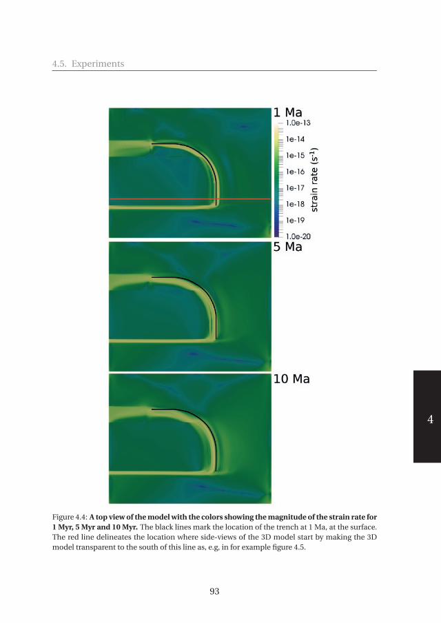
530578-L-sub01-bw-Fraters530578-L-sub01-bw-Fraters530578-L-sub01-bw-Fraters530578-L-sub01-bw-FratersProcessed on: 10-4-2019Processed on: 10-4-2019Processed on: 10-4-2019Processed on: 10-4-2019 PDF page: 103PDF page: 103PDF page: 103PDF page: 103
4
4.5. Experiments
Figure 4.4: A top view of the model with the colors showing the magnitude of the strain rate for1 Myr, 5 Myr and 10 Myr. The black lines mark the location of the trench at 1 Ma, at the surface.The red line delineates the location where side-views of the 3D model start by making the 3Dmodel transparent to the south of this line as, e.g, in for example figure 4.5.
93

530578-L-sub01-bw-Fraters530578-L-sub01-bw-Fraters530578-L-sub01-bw-Fraters530578-L-sub01-bw-FratersProcessed on: 10-4-2019Processed on: 10-4-2019Processed on: 10-4-2019Processed on: 10-4-2019 PDF page: 104PDF page: 104PDF page: 104PDF page: 104
4
Chapter 4. Assessing the geodynamics of strongly arcuate subduction zones:the eastern Caribbean subduction setting.
Figure 4.5: Viscosity and velocity evolution of the reference model through time. A view fromthe south to the north, where the southernmost 100 km of the model has been made transparent(see red line in figure 4.4) for location. The color scale indicates the viscosity, the arrow directionshow the the velocity direction and magnitude. Note that the arrows still point in their originalfull 3d direction and may therefore go in and out the plane of the section. The black line showsthe initial position of the slab at the base of the upper mantle and the red line shows the initialslab interface location at the base of the lithosphere.
much of the NLA slab is being dragged through the mantle, while this does nothappen for the eastern LA slab. The differential motion must be reflected inslab stress and deformation.
To investigate slab stress, we visualize the maximum shear stress magnitudeand direction in the slab in figures 4.8 and 4.9. In figure 4.8 the model is viewedtowards the north. At 1 Myr, the shear stress pattern in the NLA slab still showmuch high-amplitude variation which we attribute to a redistribution of stressrelative to the initial stage. Maximum shear stress patterns at 5 Myr and 10Myr show large similarity and show horizontal directions in the deep westernportion of the slab and away from the slab edge. This slab segment exposesoverall slab-strike parallel horizontal shear which may be explained by the ob-servation that the deep slab has moved less to the west than the top part of the
94

530578-L-sub01-bw-Fraters530578-L-sub01-bw-Fraters530578-L-sub01-bw-Fraters530578-L-sub01-bw-FratersProcessed on: 10-4-2019Processed on: 10-4-2019Processed on: 10-4-2019Processed on: 10-4-2019 PDF page: 105PDF page: 105PDF page: 105PDF page: 105
4
4.5. Experiments
Figure 4.6: Slab evolution through time for the reference model. A top view of the model wherethe surface colors indicate viscosity and where all of the model above 150 km and the tempera-tures beyond the range 600 to 1535 K have been made transparent. The arrows show the velocityfield. The red line shows the location of the slab in the reference model at the depth of 150 kmand at 1 Myr, and the black line show the location of the slab edge at 1 Myr.
95

530578-L-sub01-bw-Fraters530578-L-sub01-bw-Fraters530578-L-sub01-bw-Fraters530578-L-sub01-bw-FratersProcessed on: 10-4-2019Processed on: 10-4-2019Processed on: 10-4-2019Processed on: 10-4-2019 PDF page: 106PDF page: 106PDF page: 106PDF page: 106
4
Chapter 4. Assessing the geodynamics of strongly arcuate subduction zones:the eastern Caribbean subduction setting.
slab. Another contribution to slab deformation may be the resistance of themantle against slab dragging (Spakman et al., 2018) which here increases withdepth in the upper mantle. We will investigate the effect of mantle viscosityfurther below. In Fig. 4.8, the stress pattern in the eastern slab is seen in crosssectional view and exposes in the top half of the slab near vertical directionswhich concur with the observed vertical slab sinking of this slab segment. Infigure 4.9 the model is viewed in eastward direction and exposes the maximumshear stress pattern along strike of the eastern LA slab. Near the southern freeslab edge, we again observe the vertical shear directions of the upper part of theslab. No slab dragging occurs here and the slab sinks vertically between the sta-tionary trench and the deep portion of the slab that experiences the resistanceof increased mantle viscosity. Going to the north along the eastern LA slab, thedirection of the maximum shear stress turns quickly along slab-strike to a 45°angle with the dip direction which we attribute to the transition between therelatively stationary eastern LA slab and the NLA slab being dragged towardsthe west.
Our reference model generally shows maximum shear stress directions thathave a large slab-strike parallel component. This is in contrast with the classical’2D’ view of dip-aligned directions of slab stress (e.g. Houston, 2015). Impor-tantly, slab dragging in the geometrical framework of arcuate subduction offersan explanation for the observed but, as yet poorly explained, slab-strike paral-lel horizontal components of earthquake slip (e.g. Myhill, 2012; Houston, 2015;Christova, 2015), which deserves further exploration by numerical modelling.
4.5.2 The influence of the crustal rheology of the subducting plateThe crust of the NSAM plate is subducted along the LA trench. Its rheologi-
cal strength is tuned to lubricate the subduction channel but if stronger/weakerit may also cause strong shear coupling/decoupling with the overriding Caribbeanplate. In this experiment we change the strength of the subducting crust bychanging the activation energy of the dislocation creep relative to that of thereference model. This change is equally applied to crust of the ’green’ weakzones that serve to (de-)couple lateral plate motion (see figure 4.2, top). In fig-ure 4.10 the effects on plate coupling and slab evolution are shown for the east-ern LA slab. Between the strongest and weakest crust, the difference in positionof the base of the subduction channel is about 35 km. A stronger subductingcrust increases plate coupling and leads to trench advance accommodated byinternal EW-deformation of the overriding plate. A too weak crustal strengthleads to some slab rollback and increases the tendency of the slab to sink ver-tically and in the extreme case may lead to slab detachment. The tendency to
96
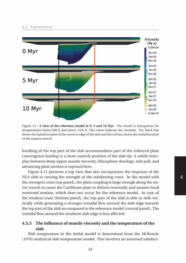
530578-L-sub01-bw-Fraters530578-L-sub01-bw-Fraters530578-L-sub01-bw-Fraters530578-L-sub01-bw-FratersProcessed on: 10-4-2019Processed on: 10-4-2019Processed on: 10-4-2019Processed on: 10-4-2019 PDF page: 107PDF page: 107PDF page: 107PDF page: 107
4
4.5. Experiments
Figure 4.7: A view of the reference model at 0, 5 and 10 Myr. The model is transparent fortemperatures below 600 K and above 1535 K. The colors indicate the viscosity. The black lineshows the initial location of the western edge of the slab and the red line shows the initial locationof the eastern trench.
buckling of the top part of the slab accommodates part of the enforced plateconvergence leading to a more easterly position of the slab tip. A subtle inter-play between deep-upper mantle viscosity, lithosphere rheology, slab pull, andadvancing plate motion is exposed here.
Figure 4.11 presents a top view that also incorporates the response of theNLA slab to varying the strength of the subducting crust. In the model withthe strongest crust (top panel), the plate coupling is large enough along the en-tire trench to cause the Caribbean plate to deform internally and assume localwestward motion, which does not occur for the reference model. In case ofthe weakest crust (bottom panel), the top part of the slab is able to sink ver-tically while generating a stronger toroidal flow around the slab edge towardsthe top part of the slab as compared to the reference model (central panel). Thetoroidal flow around the southern slab edge is less affected.
4.5.3 The influence of mantle viscosity and the temperature of theslab
Slab temperature in the initial model is determined from the McKenzie(1970) analytical slab temperature model. This involves an assumed subduct-
97

530578-L-sub01-bw-Fraters530578-L-sub01-bw-Fraters530578-L-sub01-bw-Fraters530578-L-sub01-bw-FratersProcessed on: 10-4-2019Processed on: 10-4-2019Processed on: 10-4-2019Processed on: 10-4-2019 PDF page: 108PDF page: 108PDF page: 108PDF page: 108
4
Chapter 4. Assessing the geodynamics of strongly arcuate subduction zones:the eastern Caribbean subduction setting.
Figure 4.8: Maximum shear stress through time. The direction and magnitude of maximumshear stress visualized by the cylinders as viewed from the south. For reference, a partially trans-parent colored mesh of figure 4.7 has been added.
98

530578-L-sub01-bw-Fraters530578-L-sub01-bw-Fraters530578-L-sub01-bw-Fraters530578-L-sub01-bw-FratersProcessed on: 10-4-2019Processed on: 10-4-2019Processed on: 10-4-2019Processed on: 10-4-2019 PDF page: 109PDF page: 109PDF page: 109PDF page: 109
4
4.5. Experiments
Figure 4.9: Maximum shear stress through time. The direction and magnitude of maximumshear stress visualized by the cylinders as viewed from the west. For reference, a partially trans-parent colored mesh of figure 4.7 has been added.
99

530578-L-sub01-bw-Fraters530578-L-sub01-bw-Fraters530578-L-sub01-bw-Fraters530578-L-sub01-bw-FratersProcessed on: 10-4-2019Processed on: 10-4-2019Processed on: 10-4-2019Processed on: 10-4-2019 PDF page: 110PDF page: 110PDF page: 110PDF page: 110
4
Chapter 4. Assessing the geodynamics of strongly arcuate subduction zones:the eastern Caribbean subduction setting.
Figure 4.10: Effects of variation of crustal strength. Three model results are shown for the east-ern LA slab that have been obtained for three different crustal strengths, as parameterized bythe dislocation activation energy (naqds; m3/mol). The black line lines up with the location ofthe tip of the slab and the red line lines up with the base of the subduction channel, both in themodel with strongest (223e3) crust.
ing plate velocity, called here the past plate velocity (ppv), that controls thedown-dip advection of slab temperature in the McKenzie model. Here wechange the reference model ppv value of 1.5 cm/yr to 3 cm/yr leading to acolder slab with an overall stronger slab rheology as can be seen in figure4.12. The stronger slab counteracts the tendency for slab buckling leading to aslightly straighter slab geometry as compared to the reference model slab 4.12.
In 6 modelling experiments, we combined these two initial slab-temperaturemodels with a mantle rheology that is weaker, or stronger than in the referencemodel. The overall strength of composite mantle viscosity was determined byonly changing the diffusion creep activation volume from the reference modelvalue of 5e-6 m3/mol by a value of 1e-6 m3/mol, keeping all other rheologi-
100
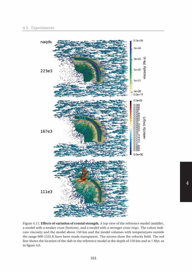
530578-L-sub01-bw-Fraters530578-L-sub01-bw-Fraters530578-L-sub01-bw-Fraters530578-L-sub01-bw-FratersProcessed on: 10-4-2019Processed on: 10-4-2019Processed on: 10-4-2019Processed on: 10-4-2019 PDF page: 111PDF page: 111PDF page: 111PDF page: 111
4
4.5. Experiments
Figure 4.11: Effects of variation of crustal strength. A top view of the reference model (middle),a model with a weaker crust (bottom), and a model with a stronger crust (top). The colors indi-cate viscosity and the model above 150 km and the model volumes with temperatures outsidethe range 600-1535 K have been made transparent. The arrows show the velocity field. The redline shows the location of the slab in the reference model at the depth of 150 km and at 1 Myr, asin figure 4.6.
101

530578-L-sub01-bw-Fraters530578-L-sub01-bw-Fraters530578-L-sub01-bw-Fraters530578-L-sub01-bw-FratersProcessed on: 10-4-2019Processed on: 10-4-2019Processed on: 10-4-2019Processed on: 10-4-2019 PDF page: 112PDF page: 112PDF page: 112PDF page: 112
4
Chapter 4. Assessing the geodynamics of strongly arcuate subduction zones:the eastern Caribbean subduction setting.
Figure 4.12: Effect of slab temperature. Figure layout as in figure 4.5. The left panels show thereference model, and the right panels show the ’cold’ model with a ppv of 3 cm/yr. The toppanels shows the temperature of the initial model, and the bottom panels shows the viscosity incolors and velocity in arrows after 10 Myr. See text for details.
cal settings of the reference model. In figure 4.13 six models are shown for thetwo levels of slab strength and 3 levels of mantle strength. The first notableeffect is that a stronger mantle provides more viscous resistance to westwardslab dragging as shown by the more eastward position of the slab near the 660as compared to the weaker mantle cases. The second effect is that the entireslab sinks to larger depth in weaker mantle which results from the decreasedviscous slab-mantle coupling. The difference in slab depth is 75-100 km be-tween the strongest and weakest mantle. The third effect is that the southernedge of the slab just above 660 km has moved 60 km more to the west in the caseof the weak mantle, as compared to the strong mantle. On the north side, theslab tip (of the south-dipping slab) is more or less at the same location. Lastly,the overall patterns of directions of maximum shear stress are comparable, butnot the magnitudes. The colder slab can carry larger-amplitude stress, while aweaker mantle allows for more slab deformation associated with higher levelsof slab stress.
These experiments demonstrate that slab dragging and the associated slabstress field are robust features with respect to the variations in slab tempera-ture and in overall mantle viscosity. In addition, slab morphology (seismolog-ical observations) and slab stress (earthquake mechanism observations) maybe important diagnostics for the dynamic state of arcuate subduction systemsthat involve slab dragging.
4.5.4 The influence of vertical weak zones in the slabThe Geodynamic World Builder facilitates making changes to the 3D initial
model. Here we replace a vertical slab segment by much weaker material (as
102

530578-L-sub01-bw-Fraters530578-L-sub01-bw-Fraters530578-L-sub01-bw-Fraters530578-L-sub01-bw-FratersProcessed on: 10-4-2019Processed on: 10-4-2019Processed on: 10-4-2019Processed on: 10-4-2019 PDF page: 113PDF page: 113PDF page: 113PDF page: 113
4
4.5. Experiments
Figure 4.13: Effect of mantle and slab strength. A north-directed view, as in figure 4.7, of 6slab models overlain by maximum shear stress directions as in figure 4.8. The left panels showmodels starting from the initial slab temperature of the reference model. The panels on the rightshow models computed with the colder initial slab of Fig. 4.12. The top row of panels showsmodels with a stronger overall upper mantle rheology defined by only changing the referencemodel diffusion creep activation volume to 6e-6 m3/mol, the center panels show models basedon the reference model rheology with a diffusion creep activation volume value of 5e-6 m3/mol,and the bottom panels show models having the weakest mantle resulting involving the diffusioncreep activation volume of 4e-6 m3/mol. The black and red lines are plotted at exactly the samelocation in each model for cross-reference.
indicated in Fig. 4.2) to test for slab deformation during subduction evolution.The vertical weak zone is implemented by replacing the crust and mantle rhe-ology of a specific GWB part of the slab by a much weaker rheology, decreas-ing the local slab strength by about 2 orders of magnitude. We inserted suchslab weakness at three different places. The results (3D viscosity and velocityfield) after 10 Myr of model evolution are shown in figure 4.14. The presenceof a weak zone in the slab does not have a large influence on the overall slabevolution. The weak zone is, to first order, advected with the stronger ambientslab. One cause for this is that at the surface, the lithosphere of the subduct-ing NSAM plate is defined to be rather strong (typically 1024-1025 Pas) whichdoes not allow for much lateral intra-plate deformation, implying that the lat-
103

530578-L-sub01-bw-Fraters530578-L-sub01-bw-Fraters530578-L-sub01-bw-Fraters530578-L-sub01-bw-FratersProcessed on: 10-4-2019Processed on: 10-4-2019Processed on: 10-4-2019Processed on: 10-4-2019 PDF page: 114PDF page: 114PDF page: 114PDF page: 114
4
Chapter 4. Assessing the geodynamics of strongly arcuate subduction zones:the eastern Caribbean subduction setting.
eral width of the weak zone in the top of the slab is largely preserved. Similarly,with increasing depth the strength of the weak zone slowly increases, followinga similar trend in the stronger adjacent slab, which causes that also in the deepupper mantle lateral slab deformation is hampered. More generally, this indi-cates that the lateral rheological strength of the subducting plate may stronglycontrol the lateral deformation of the slab during arcuate subduction.
Although the lateral slab deformation is restricted, we can observe variableslab sinking, i.e. associated with vertical slab deformation, that correlates withthe position of the inserted vertical weakness. This is best exposed by the lat-eral mantle velocity field under the Caribbean plate as can be inspected fromfigure 4.14 which exposes for each model different patterns of strong mantleflow towards the NLA slab. This flow is forced by the slab geometry change dueto differential vertical slab sinking as was observed in our reference model forthe NLA (Fig. 4.6) and SLA slabs (Fig. 4.5) and is amplified when the strength ofthe subducted crust is reduced (Fig. 4.10). A vertical weak zone in the slab leadsto sufficient decoupling of the adjacent slab segments to facilitate differentialslab sinking. Associated small slab geometry changes relative to the referencemodel slab (top panel; Fig. 4.6) can be identified in figure 4.14 where the redreference line follows the core of the reference slab. The closer the weak zoneis located towards the western slab, the more slab sinking is accommodatedby a laterally smaller segment of the slab. More detailed models and longermodel evolution are required to investigate if inherited slab weakness may leadto vertical slab segmentation resulting from differential vertical and/or hori-zontal slab motion, as proposed for the NLA slab (Harris et al., 2018). In con-trast, the eastern trench is not sensitive to the presence of a weak zone in theslab.
4.5.5 The influence of the subducting plate velocityIn this section we investigate the effect of doubling the NSAM plate velocity
to 3 cm/yr to investigate its role in the geodynamic evolution of the arcuateslab. The initial temperature model of the slab is based on a ppv of 3 cm/yr asin Fig. 4.12, while the overall rheological model is that of the reference model.The resulting model, called model B, is compared to a model A based on theNSAM velocity of 1.5 cm/yr and also on a ppv of 3 cm/yr. We compare the slabin model A at stages 10 Myr and 20 Myr with the slab in model B at 5 Myr and 10Myr of evolution, respectively, such that an equal amount of plate convergencehas occurred at each of the two stages of slab evolution.
Figure 4.15 shows the slab at these two comparable stages of evolution. Themain inference is that slab geometry at these two stages is highly comparable
104

530578-L-sub01-bw-Fraters530578-L-sub01-bw-Fraters530578-L-sub01-bw-Fraters530578-L-sub01-bw-FratersProcessed on: 10-4-2019Processed on: 10-4-2019Processed on: 10-4-2019Processed on: 10-4-2019 PDF page: 115PDF page: 115PDF page: 115PDF page: 115
4
4.5. Experiments
Figure 4.14: Effects of vertical weak zones in the slab. A top view of 4 models at 10 Myr, whichdiffer by the presence and location of a weak zone in the slab. The surface colors indicate viscos-ity and where all of models above 150 km and the temperatures outside the range 600 to 1535 Khave been made transparent. The arrows show the velocity field of the model. The curved redline shows the location of the slab without a weak zone.
105
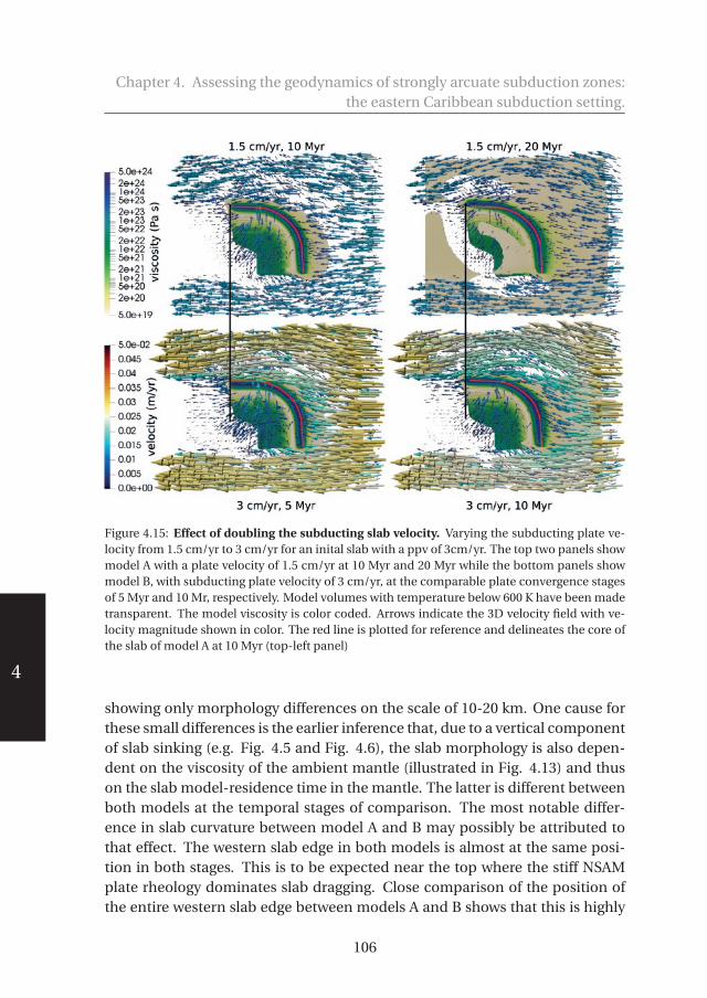
530578-L-sub01-bw-Fraters530578-L-sub01-bw-Fraters530578-L-sub01-bw-Fraters530578-L-sub01-bw-FratersProcessed on: 10-4-2019Processed on: 10-4-2019Processed on: 10-4-2019Processed on: 10-4-2019 PDF page: 116PDF page: 116PDF page: 116PDF page: 116
4
Chapter 4. Assessing the geodynamics of strongly arcuate subduction zones:the eastern Caribbean subduction setting.
Figure 4.15: Effect of doubling the subducting slab velocity. Varying the subducting plate ve-locity from 1.5 cm/yr to 3 cm/yr for an inital slab with a ppv of 3cm/yr. The top two panels showmodel A with a plate velocity of 1.5 cm/yr at 10 Myr and 20 Myr while the bottom panels showmodel B, with subducting plate velocity of 3 cm/yr, at the comparable plate convergence stagesof 5 Myr and 10 Mr, respectively. Model volumes with temperature below 600 K have been madetransparent. The model viscosity is color coded. Arrows indicate the 3D velocity field with ve-locity magnitude shown in color. The red line is plotted for reference and delineates the core ofthe slab of model A at 10 Myr (top-left panel)
showing only morphology differences on the scale of 10-20 km. One cause forthese small differences is the earlier inference that, due to a vertical componentof slab sinking (e.g. Fig. 4.5 and Fig. 4.6), the slab morphology is also depen-dent on the viscosity of the ambient mantle (illustrated in Fig. 4.13) and thuson the slab model-residence time in the mantle. The latter is different betweenboth models at the temporal stages of comparison. The most notable differ-ence in slab curvature between model A and B may possibly be attributed tothat effect. The western slab edge in both models is almost at the same posi-tion in both stages. This is to be expected near the top where the stiff NSAMplate rheology dominates slab dragging. Close comparison of the position ofthe entire western slab edge between models A and B shows that this is highly
106

530578-L-sub01-bw-Fraters530578-L-sub01-bw-Fraters530578-L-sub01-bw-Fraters530578-L-sub01-bw-FratersProcessed on: 10-4-2019Processed on: 10-4-2019Processed on: 10-4-2019Processed on: 10-4-2019 PDF page: 117PDF page: 117PDF page: 117PDF page: 117
4
4.6. Discussion and conclusions
comparable with differences in position at depth not exceeding 10 km. As weobserved earlier (Fig. 4.6 and Fig. 4.7), the deep slab tip of the western edge inthe reference model has been dragged by 50 km less to the west during 10 Myrof slab evolution. This is due to the mantle resistance against slab dragging andresistance of the slab against lateral deformation and the effect is similar for thestiffer slab of model A as can be inferred from Fig. 4.13 where the end-stages ofthe reference slab and the stiffer slab are highly comparable. The observationthat the western slab edge in model B, at 5 and 10 My, is almost at the same po-sition as in model A at 10 Myr and 20 Myr, respectively, leads to the importantimplication that doubling the absolute plate (dragging) motion of the subduct-ing plate effectively increases the mantle resistance against slab dragging in thedeeper upper mantle. We did not investigate the precise nature of the mantleresistance against slab dragging which can be a combination of the interactionof the base of the slab with the more viscous lower mantle and the viscous cou-pling between the slab and ambient upper mantle.
4.6 Discussion and conclusionsWe assessed first-order geodynamic characteristics of strongly arcuate sub-
duction systems for which we took the plate tectonic setting of the Lesser An-tilles subduction as the natural example. We took an advanced subductionstage as starting point which was the relatively well-constrained plate tectonicsetting of the Lesser Antilles trench at 10 Ma (e.g. van Benthem et al., 2014;Boschman et al., 2014). With the Geodynamic World Builder (Fraters et al.,2019b)(Chapter 3), we constructed the 3D slab following the arcuate trench-geometry and with a lateral slab curvature based on present-day tomography(Harris et al., 2018). The slab geometry is not necessarily correct but definesa starting point for modelling the evolution of arcuate subduction. Our nu-merical subduction experiments are conducted with the open source ASPECTcode and are particularly based on the implementation of composite nonlin-ear visco-plastic rheologies (Glerum et al., 2018) and on the faster and stableconvergence provided by the Newton method (Fraters et al., 2019a)(Chapter 2).
We particularly designed our experiments for a "90°"-arcuate subductionsetting that combines trench-perpendicular subducting-plate convergence ata mantle-stationary trench along one side of the system with trench-parallelsubducting-plate motion occurring at a mantle-stationary trench along theother side. This geodynamic setting defined the reference subduction modelfor which we showed in various experiments that the main dynamic features ofmodelled arcuate subduction evolution are robust with respect to realistic vari-ations of the kinematic settings and of the rheological crust-mantle properties.
107

530578-L-sub01-bw-Fraters530578-L-sub01-bw-Fraters530578-L-sub01-bw-Fraters530578-L-sub01-bw-FratersProcessed on: 10-4-2019Processed on: 10-4-2019Processed on: 10-4-2019Processed on: 10-4-2019 PDF page: 118PDF page: 118PDF page: 118PDF page: 118
4
Chapter 4. Assessing the geodynamics of strongly arcuate subduction zones:the eastern Caribbean subduction setting.
Foremost, our simulations of 10 Myr, in one case 20 Myr, of subduction evo-lution demonstrated that slab dragging, i.e. lateral transport of the lithosphereslab by the surface motion of the subducting plate, is a geodynamically feasi-ble process that leads to internal slab deformation but not necessarily to im-mediate slab tearing or destruction of the arcuate nature in other ways. Slabdragging is demonstrated for a large subduction system with an arcuate slabacross the entire upper mantle involving a more than ∼2000 km long trenchand for trench-parallel dragging velocities of 15 and 30 mm/yr during 10-20Myr, involving trench-parallel slab transport by 150-300 km for the top of theslab. Earlier assessments of the geodynamical feasibility of slab dragging con-cerned relative short (< 200 km) and laterally small (∼100 km) slab ’stumps’ be-ing dragged by the Pacific plate under the western NAM plate boundary (Pikseret al., 2012) and the isolated, about 200-300 km wide, Gibraltar slab across theupper mantle of the westernmost Mediterranean (Spakman et al., 2018). Here,the application to eastern Caribbean subduction demonstrates that the over-all slab geometry obtained after 10 My of evolution conforms with the tomo-graphic images of the present-day LA slab, which agrees with the hypothesisthat westward slab dragging, involving the slab across the entire upper-mantle,occurs along the northern LA trench.
A next key observation is that slab dragging is resisted by the slab and man-tle involving two dynamic effects. The first effect is the viscous mantle resis-tance against slab dragging, which was demonstrated in experiments using aweaker or stronger mantle rheology relative to the reference model. The sec-ond effect involves resistance of the slab itself against slab dragging. This ismore of a geometrical nature and is here caused by the geodynamic setting inwhich the northern slab is moving away from the eastern slab. This implies lat-erally distributed deformation of the slab which is associated with a complex3D stress field. We visualized the stress field by showing the magnitudes and di-rections of the maximum shear stress. For rheologically isotropic media, as wemodel here, such directions indicate candidate directions of earthquake fault-slip. We conclude from our experiments that slab dragging sets up a complexslab stress field characterized by strong deviations in the slab stress orienta-tion from the more classical view of maximum stress directions parallel to thetrench-perpendicular slab-dip plane. Particularly, we noticed horizontal slab-strike parallel maximum directions of shear stress in the northern slab whichwe relate to the bulk horizontal-shear deformation by 50 km across the entireupper-mantle slab that occurred during 10 Myr of slab dragging with 15 mm/yr.The generally off-dip directions of maximum shear stress explain observations
108

530578-L-sub01-bw-Fraters530578-L-sub01-bw-Fraters530578-L-sub01-bw-Fraters530578-L-sub01-bw-FratersProcessed on: 10-4-2019Processed on: 10-4-2019Processed on: 10-4-2019Processed on: 10-4-2019 PDF page: 119PDF page: 119PDF page: 119PDF page: 119
4
4.6. Discussion and conclusions
of slab-strike parallel slip components inferred from focal mechanisms of in-termediate and deep earthquakes (e.g. Giardini and Woodhouse, 1986; Myhilland Warren, 2012; Houston, 2015; Christova, 2015; Meighan et al., 2013).
Slab stress and deformation due to slab dragging are transmitted into theupper plate where it leads to crustal deformation (Spakman et al., 2018). Mod-elling the tectonic response to slab dragging was not our goal, but in our refer-ence model we did infer a first-order effect of upper plate deformation directlysouth of the northern trench, which concurs in location with the observed up-per plate deformation along the NLA plate boundary (e.g. Calais et al., 2016).
Our work realizes an important step towards the numerical simulation ofnatural subduction by demonstrating the (open source) capabilities and com-putational feasibility of assessing the first-order geodynamic features associ-ated with natural (arcuate) subduction such that the next step of detailed mod-elling of the tectonic evolution of the overlying crust is now within reach.
109

530578-L-sub01-bw-Fraters530578-L-sub01-bw-Fraters530578-L-sub01-bw-Fraters530578-L-sub01-bw-FratersProcessed on: 10-4-2019Processed on: 10-4-2019Processed on: 10-4-2019Processed on: 10-4-2019 PDF page: 120PDF page: 120PDF page: 120PDF page: 120
4
Chapter 4. Assessing the geodynamics of strongly arcuate subduction zones:the eastern Caribbean subduction setting.
4.7 Appendix A: GWB inputThe reference world builder input file is given in listing 4.1. Colder slabs are
made through higher velocity in the temperature model of the slab. Note thatthe notation of version 0.2.0 of the GWB would be a lot shorter. See listing 3.13for an example which is written for version 0.2.0 and which has a very similarinitial setting. The weak zones are created by adding one of the three listingsbetween the subducting slab and South Weakzone featrues: listing 4.2 for thewestern fault, listing 4.3 for the centeral fault and listing 4.4 for the eastern fault.
1 {2 "version":"0.1",3 "potential mantle temperature":1500,4 "thermal expansion coefficient":2.0e-5,5 "minimum points per distance":100000 ,6 "interpolation":"monotone spline",7 "coordinate system":{"cartesian":{}},8 "features":9 {
10 "oceanic plate":{"name":"NS American plate",11 "coordinates":12 [[1700e3 ,0] ,[1700e3 ,300e3] ,[1689e3 ,422e3] ,[1658e3 ,539e3],13 [1606e3 ,650e3] ,[1536e3 ,749e3] ,[1450e3 ,836e3] ,[1350e3 ,906e3],14 [1239e3 ,958e3] ,[1122e3 ,989e3] ,[1000e3 ,1000e3],[-1e3 ,1000e3],15 [-1e3 ,1501 e3] ,[2501e3 ,1501 e3] ,[2501e3 ,-501e3],[-1e3 ,-501e3],16 [-1e3 ,-50e3] ,[2000e3 ,-50e3] ,[2000e3 ,0e3]],17 "temperature model":{"name":"linear", "depth":100e3},18 "composition model":19 {"name":"constant layers", "depth":100e3,20 "layers":[{"compositions":[0], "thickness":30e3}]}},2122 "oceanic plate":{"name":"Caribbean plate",23 "coordinates":24 [[1700e3 ,300e3] ,[1689e3 ,422e3] ,[1658e3 ,539e3] ,[1606e3 ,650e3],25 [1536e3 ,749e3] ,[1450e3 ,836e3] ,[1350e3 ,906e3] ,[1239e3 ,958e3],26 [1122e3 ,989e3] ,[1000e3 ,1000e3],[650e3 ,1000e3],[-1e3 ,1000e3],27 [-1e3 ,0e3] ,[1700e3 ,0e3]],28 "temperature model":{"name":"linear", "depth":100e3},29 "composition model":30 {"name":"constant layers", "depth":100e3,31 "layers":[{"compositions":[1], "thickness":30e3}]}},3233 "continental plate":{"name":"Caribbean weak zone",34 "coordinates":35 [[-1e3 ,1000 e3],[-1e3 ,750e3] ,[1536e3 ,749e3] ,[1450e3 ,836e3],36 [1350e3 ,906e3] ,[1239e3 ,958e3] ,[1122e3 ,989e3] ,[1000e3 ,1000 e3],37 [650e3 ,1000 e3]],38 "temperature model":{"name":"linear", "depth":100e3},39 "composition model":40 {"name":"constant layers", "depth":100e3,41 "layers":[{"compositions":[2], "thickness":30e3},42 {"compositions":[3], "thickness":70e3}]}},4344 "mantle layer":{"name":"upper mantle", "top depth":100e3,45 "coordinates":46 [[-1e3 ,-500e3],[-501e3 ,2500 e3] ,[2501e3 ,2500 e3] ,[2501e3 ,-501e3]],47 "temperature model":{"name":"none"},48 "composition model":{"name":"none"}},4950 "mantle layer":{"name":"660", "top depth":660e3,51 "coordinates":
110

530578-L-sub01-bw-Fraters530578-L-sub01-bw-Fraters530578-L-sub01-bw-Fraters530578-L-sub01-bw-FratersProcessed on: 10-4-2019Processed on: 10-4-2019Processed on: 10-4-2019Processed on: 10-4-2019 PDF page: 121PDF page: 121PDF page: 121PDF page: 121
4
4.7. Appendix A: GWB input
52 [[-1e3 ,-500e3],[-501e3 ,2500 e3] ,[2501e3 ,2500 e3] ,[2501e3 ,-501e3]],53 "temperature model":{"name":"none"},54 "composition model":55 {"name":"constant", "depth":200e3, "compositions":[4]}} ,5657 "subducting plate":{"name":"Lesser Antilles slab",58 "coordinates":59 [[1700e3 ,0] ,[1700e3 ,300e3] ,[1689e3 ,422e3] ,[1658e3 ,539e3],60 [1606e3 ,650e3] ,[1536e3 ,749e3] ,[1450e3 ,836e3] ,[1350e3 ,906e3],61 [1239e3 ,958e3] ,[1122e3 ,989e3] ,[1000e3 ,1000e3] ,[650e3 ,1000 e3]],62 "reference point":[-1,-1],63 "starting depth":0, "maximum depth":660e3 ,64 "segments":65 {66 "all":[{"length":150e3 , "thickness":[100e3], "angle":[0 ,25]} ,67 {"length":150e3 , "thickness":[100e3], "angle":[25 ,50]} ,68 {"length":371e3 , "thickness":[100e3], "angle":[50]} ,69 {"length":300e3 , "thickness":[100e3], "angle":[50 ,0]},70 {"length":0, "thickness":[100e3], "angle":[0]}] ,71 "1":[{"length":150e3, "thickness":[100e3], "angle":[0,25]},72 {"length":150e3 , "thickness":[100e3], "angle":[25 ,50]} ,73 {"length":371e3 , "thickness":[100e3], "angle":[50]} ,74 {"length":275e3 , "thickness":[100e3], "angle":[50 ,0]},75 {"length":0, "thickness":[100e3], "angle":[0]}] ,76 "2":[{"length":150e3, "thickness":[100e3], "angle":[0,25]},77 {"length":150e3 , "thickness":[100e3], "angle":[25 ,50]} ,78 {"length":371e3 , "thickness":[100e3], "angle":[50]} ,79 {"length":275e3 , "thickness":[100e3], "angle":[50 ,0]},80 {"length":0, "thickness":[100e3], "angle":[0]}] ,81 "3":[{"length":150e3, "thickness":[100e3], "angle":[0,25]},82 {"length":150e3 , "thickness":[100e3], "angle":[25 ,50]} ,83 {"length":371e3 , "thickness":[100e3], "angle":[50]} ,84 {"length":275e3 , "thickness":[100e3], "angle":[50 ,0]},85 {"length":0, "thickness":[100e3], "angle":[0]}] ,86 "4":[{"length":150e3, "thickness":[100e3], "angle":[0,25]},87 {"length":150e3 , "thickness":[100e3], "angle":[25 ,50]} ,88 {"length":371e3 , "thickness":[100e3], "angle":[50]} ,89 {"length":275e3 , "thickness":[100e3], "angle":[50 ,0]},90 {"length":0e3, "thickness":[100 e3], "angle":[0]}] ,91 "5":[{"length":150e3, "thickness":[100e3], "angle":[0,25]},92 {"length":150e3 , "thickness":[100e3], "angle":[25 ,50]} ,93 {"length":371e3 , "thickness":[100e3], "angle":[50]} ,94 {"length":275e3 , "thickness":[100e3], "angle":[50 ,0]},95 {"length":0, "thickness":[100e3], "angle":[0]}] ,96 "6":[{"length":150e3, "thickness":[100e3], "angle":[0,25]},97 {"length":150e3 , "thickness":[100e3], "angle":[25 ,50]} ,98 {"length":371e3 , "thickness":[100e3], "angle":[50]} ,99 {"length":275e3 , "thickness":[100e3], "angle":[50 ,0]},
100 {"length":0, "thickness":[100e3], "angle":[0]}] ,101 "7":[{"length":150e3, "thickness":[100e3], "angle":[0,25]},102 {"length":150e3 , "thickness":[100e3], "angle":[25 ,50]} ,103 {"length":371e3 , "thickness":[100e3], "angle":[50]} ,104 {"length":275e3 , "thickness":[100e3], "angle":[50 ,0]},105 {"length":0, "thickness":[100e3], "angle":[0]}] ,106 "8":[{"length":150e3, "thickness":[100e3], "angle":[0,25]},107 {"length":150e3 , "thickness":[100e3], "angle":[25 ,50]} ,108 {"length":371e3 , "thickness":[100e3], "angle":[50]} ,109 {"length":275e3 , "thickness":[100e3], "angle":[50 ,0]},110 {"length":0, "thickness":[100e3], "angle":[0]}] ,111 "9":[{"length":150e3, "thickness":[100e3], "angle":[0,25]},112 {"length":150e3 , "thickness":[100e3], "angle":[25 ,50]} ,113 {"length":371e3 , "thickness":[100e3], "angle":[50]} ,114 {"length":275e3 , "thickness":[100e3], "angle":[50 ,0]},115 {"length":0, "thickness":[100e3], "angle":[0]}] ,116 "10":[{"length":150e3, "thickness":[100 e3], "angle":[0,25]} ,
111

530578-L-sub01-bw-Fraters530578-L-sub01-bw-Fraters530578-L-sub01-bw-Fraters530578-L-sub01-bw-FratersProcessed on: 10-4-2019Processed on: 10-4-2019Processed on: 10-4-2019Processed on: 10-4-2019 PDF page: 122PDF page: 122PDF page: 122PDF page: 122
4
Chapter 4. Assessing the geodynamics of strongly arcuate subduction zones:the eastern Caribbean subduction setting.
117 {"length":150e3 , "thickness":[100e3], "angle":[25 ,50]} ,118 {"length":371e3 , "thickness":[100e3], "angle":[50]} ,119 {"length":275e3 , "thickness":[100e3], "angle":[50 ,0]},120 {"length":0, "thickness":[100e3], "angle":[0]}] ,121 "11":[{"length":150e3, "thickness":[100 e3], "angle":[0,25]},122 {"length":150e3 , "thickness":[100e3], "angle":[25 ,50]} ,123 {"length":371e3 , "thickness":[100e3], "angle":[50]} ,124 {"length":50e3 , "thickness":[100e3], "angle":[50,0]} ,125 {"length":0, "thickness":[100e3], "angle":[0]}]126 },127 "temperature model":128 {"name":"plate model", "density":3300, "plate velocity":0.0150 ,129 "thermal conductivity":2.5, "thermal expansion coefficient":2e-5 },130 "composition model":131 {"name":"constant layers",132 "layers":[{"compositions":[0], "thickness":30e3},133 {"compositions":[0], "fractions":[0], "thickness":70e3}]}},134135 "continental plate":{"name":"South Weakzone",136 "coordinates":[[-1e3 ,0e3],[-1e3 ,-50e3] ,[2000e3 ,-50e3] ,[2000e3 ,0e3]],137 "temperature model":{"name":"linear", "depth":100e3},138 "composition model":{"name":"constant layers", "depth":100e3,139 "layers":[{"compositions":[2], "thickness":30e3},140 {"compositions":[3], "thickness":70e3}]}}141 }142 }
Listing 4.1: The reference GWB input file
1 "oceanic plate": {"name":"Compositional Western plate Fault",2 "coordinates":[[1239e3 ,958e3] ,[1122e3 ,989e3] ,[1232e3 ,1167e3]],3 "temperature model":{"name":"none"},4 "composition model":{"name":"constant layers",5 "layers":[{"compositions":[2], "thickness":30e3},6 {"compositions":[3], "thickness":70e3}]}},78 "subducting plate":{"name":"Compositional Western slab Fault",9 "coordinates":[[1239e3 ,958e3] ,[1122e3 ,989e3]], "reference point":[-1,-1],
10 "segments":{11 "all":[{"length":150e3 , "thickness":[100 e3], "angle":[0 ,25]} ,12 {"length":150e3 , "thickness":[100e3], "angle":[25 ,50]} ,13 {"length":371e3 , "thickness":[100e3], "angle":[50]} ,14 {"length":275e3 , "thickness":[100e3], "angle":[50 ,0]}]} ,15 "temperature model":{"name":"none"},16 "composition model":{"name":"constant layers",17 "layers":[{"compositions":[2], "thickness":30e3},18 {"compositions":[3], "thickness":70e3}]}},
Listing 4.2: The addition to the reference GWB input file needed to create the western slabweakzone.
1 "oceanic plate": {"name":"Compositional Western plate Fault",2 "coordinates":[[1536e3 ,749e3] ,[1450e3 ,836e3] ,[1635e3 ,932e3]],3 "temperature model":{"name":"none"},4 "composition model":{"name":"constant layers",5 "layers":[{"compositions":[2], "thickness":30e3},6 {"compositions":[3], "thickness":70e3}]}},78 "subducting plate":{"name":"Compositional Western slab Fault",9 "coordinates":[[1536e3 ,749e3] ,[1450e3 ,836e3]], "reference point":[-1,-1],
10 "segments":{11 "all":[{"length":150e3 , "thickness":[100 e3], "angle":[0 ,25]} ,12 {"length":150e3 , "thickness":[100e3], "angle":[25 ,50]} ,
112

530578-L-sub01-bw-Fraters530578-L-sub01-bw-Fraters530578-L-sub01-bw-Fraters530578-L-sub01-bw-FratersProcessed on: 10-4-2019Processed on: 10-4-2019Processed on: 10-4-2019Processed on: 10-4-2019 PDF page: 123PDF page: 123PDF page: 123PDF page: 123
4
4.8. Appendix B: ASPECT intput
13 {"length":371e3 , "thickness":[100e3], "angle":[50]} ,14 {"length":275e3 , "thickness":[100e3], "angle":[50 ,0]}]} ,15 "temperature model":{"name":"none"},16 "composition model":{"name":"constant layers",17 "layers":[{"compositions":[2], "thickness":30e3},18 {"compositions":[3], "thickness":70e3}]}},
Listing 4.3: The addition to the reference GWB input file needed to create the central slabweakzone.
1 "oceanic plate": {"name":"Compositional Western plate Fault",2 "coordinates":[[1689e3 ,422e3] ,[1658e3 ,539e3] ,[1867e3 ,532e3]],3 "temperature model":{"name":"none"},4 "composition model":{"name":"constant layers",5 "layers":[{"compositions":[2], "thickness":30e3},6 {"compositions":[3], "thickness":70e3}]}},78 "subducting plate":{"name":"Compositional Western slab Fault",9 "coordinates":[[1689e3 ,422e3] ,[1658e3 ,539e3]], "reference point":[-1,-1],
10 "segments":{11 "all":[{"length":150e3, "thickness":[100 e3], "angle":[0 ,25]} ,12 {"length":150e3 , "thickness":[100e3], "angle":[25 ,50]} ,13 {"length":371e3 , "thickness":[100e3], "angle":[50]} ,14 {"length":275e3 , "thickness":[100e3], "angle":[50 ,0]}]} ,15 "temperature model":{"name":"none"},16 "composition model":{"name":"constant layers",17 "layers":[{"compositions":[2], "thickness":30e3},18 {"compositions":[3], "thickness":70e3}]}},
Listing 4.4: The addition to the reference GWB input file needed to create the eastern slabweakzone.
4.8 Appendix B: ASPECT intput1 set World builder file = world/builder/file/location.wb2 set Output directory = aspect/output/dir/3 set Dimension = 34 set CFL number = 0.055 set Max nonlinear iterations = 506 set End time = 2e77 set Nonlinear solver scheme = iterated Advection and Newton Stokes8 set Timing output frequency = 09 set Max nonlinear iterations in pre -refinement = 0
10 set Pressure normalization = no11 set Nonlinear solver tolerance = 1e-612 set Maximum time step = 1000013 set Maximum relative increase in time step = 2514 set Maximum first time step = 1001516 subsection Solver parameters17 subsection Newton solver parameters18 set Max pre -Newton nonlinear iterations = 10019 set Nonlinear Newton solver switch tolerance = 1e-420 set Max Newton line search iterations = 021 set Maximum linear Stokes solver tolerance = 1e-122 set Use Newton residual scaling method = false23 set Use Newton failsafe = true24 set Stabilization preconditioner = SPD25 set Stabilization velocity block = SPD26 set Use Eisenstat Walker method for Picard iterations = true
113

530578-L-sub01-bw-Fraters530578-L-sub01-bw-Fraters530578-L-sub01-bw-Fraters530578-L-sub01-bw-FratersProcessed on: 10-4-2019Processed on: 10-4-2019Processed on: 10-4-2019Processed on: 10-4-2019 PDF page: 124PDF page: 124PDF page: 124PDF page: 124
4
Chapter 4. Assessing the geodynamics of strongly arcuate subduction zones:the eastern Caribbean subduction setting.
27 end28 end2930 subsection Geometry model31 set Model name = box with lithosphere boundary indicators32 subsection Box with lithosphere boundary indicators33 set X extent = 2500e334 set Y extent = 2000e335 set Z extent = 800e336 set Box origin Y coordinate = -500e337 set X repetitions = 2538 set Y repetitions = 2039 set Y repetitions lithosphere = 1040 set Z repetitions = 641 set Z repetitions lithosphere= 142 set Lithospheric thickness = 100e34344 end45 subsection Box46 set X extent = 396000047 set Y extent = 462000048 set Z extent = 66000049 set X repetitions = 650 set Y repetitions = 751 end52 subsection Ellipsoidal chunk53 set NE corner = -58:2654 set SW corner = -82:1455 set Depth = 70000056 set Semi -major axis = 637813757 set Eccentricity = 058 set East -West subdivisions = 459 set North -South subdivisions = 260 set Depth subdivisions = 161 end62 end6364 subsection Material model65 set Model name = visco plastic66 subsection Visco Plastic67 set Reference viscosity = 1.0 e2168 set Grain size = 0.0169 set Viscosity averaging scheme = harmonic70 set Minimum viscosity = 5e1971 set Maximum viscosity = 5e2472 set Reference temperature = 293 lith , lower mantle73 set Densities = 3300 3300, 330074 set Thermal expansivities = 2e-575 # Up M., NA C.,
CARBC , Wk C., Wk L., Lower Mantle76 set Prefactors for dislocation creep = 6.51e-15, 8.57e-28, 8.57e
-28, 8.57e-28, 6.51e-15, 6.51e-1677 set Stress exponents for dislocation creep = 3.5, 4.0,
4.0, 4.0, 3.8, 3.578 set Activation energies for dislocation creep = 530.e3, 167e3, 223.
e3, 167e3 , 440.e3 , 530.e379 set Activation volumes for dislocation creep = 18e-6, 36e-6, 18e
-6, 18e-6, 18e-6, 18e-680 set Prefactors for diffusion creep = 8.88e-15, 8.88e-15, 8.88e
-15, 8.88e-15, 8.88e-15, 8.88e-1581 set Activation energies for diffusion creep = 335e3 , 375e3 , 375
e3, 375e3, 335e3, 355e382 set Activation volumes for diffusion creep = 5.0e-6, 6.0e-6, 6.0e
-6, 6.0e-6, 6.0e-6, 6.0e-683
114
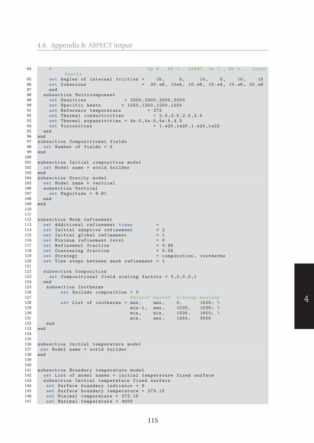
530578-L-sub01-bw-Fraters530578-L-sub01-bw-Fraters530578-L-sub01-bw-Fraters530578-L-sub01-bw-FratersProcessed on: 10-4-2019Processed on: 10-4-2019Processed on: 10-4-2019Processed on: 10-4-2019 PDF page: 125PDF page: 125PDF page: 125PDF page: 125
4
4.8. Appendix B: ASPECT intput
84 # Up M., NA C., CARBC , Wk C., Wk L., LowerMantle
85 set Angles of internal friction = 15, 5, 10, 5, 10, 1586 set Cohesions = 20.e6 , 10e4, 10.e6, 10.e4, 10.e6, 20.e687 end88 subsection Multicomponent89 set Densities = 3300 ,3300 ,3000 ,300090 set Specific heats = 1250 ,1250 ,1250 ,125091 set Reference temperature = 27392 set Thermal conductivities = 2.5 ,2.5 ,2.5 ,2.593 set Thermal expansivities = 4e-5,4e-5,4e-5 ,4.594 set Viscosities = 1.e20 ,1e20 ,1.e24 ,1e2295 end96 end97 subsection Compositional fields98 set Number of fields = 599 end
100101 subsection Initial composition model102 set Model name = world builder103 end104 subsection Gravity model105 set Model name = vertical106 subsection Vertical107 set Magnitude = 9.81108 end109 end110111112 subsection Mesh refinement113 set Additional refinement times =114 set Initial adaptive refinement = 2115 set Initial global refinement = 1116 set Minimum refinement level = 0117 set Refinement fraction = 0.95118 set Coarsening fraction = 0.05119 set Strategy = composition , isotherms120 set Time steps between mesh refinement = 1121122 subsection Composition123 set Compositional field scaling factors = 0,0,0,0,1124 end125 subsection Isotherms126 set Exclude composition = 0127 #minref maxref mintemp maxtemp128 set List of isotherms = max , max , 0, 1525; \129 min -1, max , 1525, 1535; \130 min , min , 1535, 1650; \131 min , max , 1650, 3000132 end133 end134135136 subsection Initial temperature model137 set Model name = world builder138 end139140141 subsection Boundary temperature model142 set List of model names = initial temperature fixed surface143 subsection Initial temperature fixed surface144 set Surface boundary indicator = 5145 set Surface boundary temperature = 273.15146 set Minimal temperature = 273.15147 set Maximal temperature = 4000
115

530578-L-sub01-bw-Fraters530578-L-sub01-bw-Fraters530578-L-sub01-bw-Fraters530578-L-sub01-bw-FratersProcessed on: 10-4-2019Processed on: 10-4-2019Processed on: 10-4-2019Processed on: 10-4-2019 PDF page: 126PDF page: 126PDF page: 126PDF page: 126
4
Chapter 4. Assessing the geodynamics of strongly arcuate subduction zones:the eastern Caribbean subduction setting.
148 end149 end150151 subsection Discretization152 set Use locally conservative discretization = false153 subsection Stabilization parameters154 set Use artificial viscosity smoothing = false155 set alpha = 2156 set beta = 0.078157 end158 end159160 subsection Boundary temperature model161 set Fixed temperature boundary indicators = 0,1,2,3,4,5,6,7,8,9162 end163164 subsection Boundary velocity model165 set Prescribed velocity boundary indicators = left lithosphere xyz:function ,
right lithosphere xyz:function , front lithosphere z:function , backlithosphere z:function
166 set Tangential velocity boundary indicators =167 set Zero velocity boundary indicators = bottom168 end169170 subsection Boundary traction model171 set Prescribed traction boundary indicators = front lithosphere: initial
lithostatic pressure , back lithosphere: initial lithostatic pressure ,left: initial lithostatic pressure , right: initial lithostatic pressure , back: initial lithostatic pressure , front: initial lithostatic pressure
172 end173174175 subsection Free surface176 set Free surface boundary indicators = outer177 end178179 subsection Boundary traction model180 subsection Initial lithostatic pressure181 set Representative point = 2000e3 ,750e3 ,375e3182 end183 end184185 subsection Free surface186 set Free surface stabilization theta = 0.75187 end188189 subsection Boundary velocity model190 subsection Function191 set Variable names = x,y,z,t192 set Function constants = velocity = -0.0150193 set Function expression = if(x > 1, if(y >= -300e3 ,velocity ,(abs(y+500
e3)/200e3)*0.25* velocity +0.75* velocity), if(y <= 750e3 && y >= 0, 0, if(y >= 1000e3 || y <= -50e3, velocity , if( y >= 750e3, (abs(y-750e3)/250e3)*velocity , (abs(y)/50e3)*velocity))));0;0
194 end195 end196197198 subsection Postprocess199 set List of postprocessors = visualization ,velocity statistics , composition
statistics , pressure statistics , temperature statistics200 subsection Visualization201 set Time between graphical output = 100e3202 set List of output variables = viscosity , density , strain rate ,depth ,
nonadiabatic pressure , spd factor , shear stress eigenvectors , maximum
116
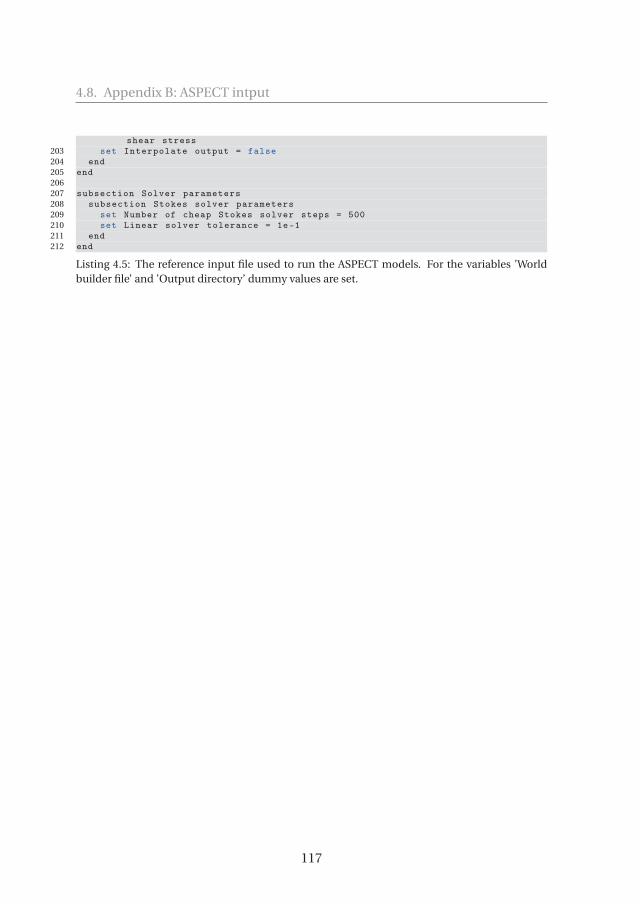
530578-L-sub01-bw-Fraters530578-L-sub01-bw-Fraters530578-L-sub01-bw-Fraters530578-L-sub01-bw-FratersProcessed on: 10-4-2019Processed on: 10-4-2019Processed on: 10-4-2019Processed on: 10-4-2019 PDF page: 127PDF page: 127PDF page: 127PDF page: 127
4.8. Appendix B: ASPECT intput
shear stress203 set Interpolate output = false204 end205 end206207 subsection Solver parameters208 subsection Stokes solver parameters209 set Number of cheap Stokes solver steps = 500210 set Linear solver tolerance = 1e-1211 end212 end
Listing 4.5: The reference input file used to run the ASPECT models. For the variables ’Worldbuilder file’ and ’Output directory’ dummy values are set.
117

530578-L-sub01-bw-Fraters530578-L-sub01-bw-Fraters530578-L-sub01-bw-Fraters530578-L-sub01-bw-FratersProcessed on: 10-4-2019Processed on: 10-4-2019Processed on: 10-4-2019Processed on: 10-4-2019 PDF page: 128PDF page: 128PDF page: 128PDF page: 128

530578-L-sub01-bw-Fraters530578-L-sub01-bw-Fraters530578-L-sub01-bw-Fraters530578-L-sub01-bw-FratersProcessed on: 10-4-2019Processed on: 10-4-2019Processed on: 10-4-2019Processed on: 10-4-2019 PDF page: 129PDF page: 129PDF page: 129PDF page: 129
5Conclusions and outlook
530578-L-sub01-bw-Fraters530578-L-sub01-bw-Fraters530578-L-sub01-bw-Fraters530578-L-sub01-bw-FratersProcessed on: 10-4-2019Processed on: 10-4-2019Processed on: 10-4-2019Processed on: 10-4-2019 PDF page: 130PDF page: 130PDF page: 130PDF page: 130
5
Chapter 5. Conclusions and outlook
In this thesis I have addressed several first-order issues that aim to con-tribute toward more efficient and effective modeling of 3D inherently compli-cated natural subduction settings. These issues define first steps opening up alarge scope of new research.
The research into implementing a Newton solver for ASPECT, as reportedin Chapter 2, was originally intended as a relatively straight-forward develop-ment. However, we identified a fundamental problem with solving the Stokesequations via a Newton solver as is used in many other FE or FD codes. Thisproblem is that the linearization for setting up the Newton method may leadto a singular matrix that prevents the solution of the Newton problem, whilethis does not occur for the usual linearization associated with Picard iteration.We have addressed this issue in an optimal manner, in the sense of fastest non-linear convergence while retaining numerical stability. This was achieved forsolving the incompressible Stokes equations, however, the singularity problemremains as yet unsolved for the compressible formulation, although we expectthat a similar approach in addressing the issue is feasible. Our solution to thesingularity problem is not restricted to ASPECT but also applicable to other FEand FD methods. Straightforward wall-time comparison between the Picardand Newton methods is problematic, because the computation time is prob-lem dependent and dependent on what nonlinear tolerance is adopted for theproblem. I have shown that for a complex 3D case, the Newton solver was sig-nificantly faster in terms of wall-time (see Chapter 2), which has been furtherenhanced by later code optimization. Currently, the Newton solver requiresderivative information related to the materials used. In the current ASPECTimplementation some material models allow for fast analytical evaluation ofderivatives whereas others require a significant amount time for computing thederivatives through finite difference. This is especially the case for the morecomplex material models such as visco-plasticity. Using analytic derivativescould lead also here to a considerable speed up of the Newton iteration.
In Chapter 3 I addressed the problem of how to create geometrically com-plex initial conditions for numerical modelling in a user-friendly, easily extend-able and easily modifiable way. To this end I developed an open source codelibrary, the Geodynamic World Builder (GWB), which allows for the creationand (Paraview) visualization of complex initial temperature and initial com-position model setups. This is realized through a simple text input-file, in theJSON language, in which users provide parameters defining tectonic featuresand their associated temperature and compositional models. The setup can beeasily changed from Cartesian to spherical coordinates and back. The library
120

530578-L-sub01-bw-Fraters530578-L-sub01-bw-Fraters530578-L-sub01-bw-Fraters530578-L-sub01-bw-FratersProcessed on: 10-4-2019Processed on: 10-4-2019Processed on: 10-4-2019Processed on: 10-4-2019 PDF page: 131PDF page: 131PDF page: 131PDF page: 131
5
has been designed to be easily integrated with geodynamic codes used by thegeodynamic modelling community. So far, it has already been successfully in-tegrated in two Fortran codes, ELEFANT and SEPRAN, and one C++ code, AS-PECT. As shown in both Chapters 3 and 4, the present version of the GWB isalready a versatile tool and ready for use but several possibilities for extensionsof this library are already envisaged. Examples are parameterization of topog-raphy/bathymetry, passive margins, variable crust and lithosphere thickness,or of mantle plumes and mantle tomography models, which all will be consid-ered in the near future. Other output possibilities can be plate velocities, forexample for use as boundary conditions. At the time that the GWB library be-comes integrated in more codes by the community and sees its user base grow,the amount of available features is expected to grow organically with the num-ber of users adding their features as were required for their own project. Whileusers and developers alike usually implement their own initial conditions fortheir specific setup and code, they have now the possibility to add it to a safeand backward-compatible numerical library for their later (re-)use, or for useby others.
In Chapter 4, I have used the advantages of the computational speedup andaccuracy of ASPECT offered by the Newton solver and the easy constructionof 3D initial conditions by the GWB, to advance research into the geodynam-ics of strongly arcuate subduction in which the slab may be dragged trench-parallel through the mantle by the surface motion of the subducting plate alongone segment of the curved trench. The plate-tectonic evolution of the stronglyarcuate eastern Caribbean subduction since 10 Ma provided the natural set-ting for this investigation. By varying various initial settings, boundary condi-tions, and parameters defining the model rheology, I demonstrated the geo-dynamic feasibility of trench-parallel dragging of the northern Lesser-Antilles(NLA) slab by plate motions between 1.5-3.0 cm/yr during the past 10 Myr and5 Myr respectively, corresponding to westward lateral slab transport of 150 km,while trench-perpendicular subduction along the eastern Lesser Antilles slabremained more or less trench stationary. The actual absolute plate motion ofthe North American plate along the NLA trench is about 2.0 cm/yr (Doubrovineet al. (2012)) and within the modelled range. The geodynamic setting impliesconsiderable internal deformation and shape change of the slab which occurson spatial scales relevant for the tectonic evolution of the plate boundary zone.In the common view, the stress field in the slab is dominantly aligned along theslab-dip direction. In the geodynamic setting of arcuate subduction where theplate convergence direction strongly changes along the trench, I generally in-
121

530578-L-sub01-bw-Fraters530578-L-sub01-bw-Fraters530578-L-sub01-bw-Fraters530578-L-sub01-bw-FratersProcessed on: 10-4-2019Processed on: 10-4-2019Processed on: 10-4-2019Processed on: 10-4-2019 PDF page: 132PDF page: 132PDF page: 132PDF page: 132
Chapter 5. Conclusions and outlook
ferred strong components of maximum shear stress oblique to dip-plane whichare associated with the along slab-strike deformation of the slab. This may linkto the occurrence of focal mechanisms of intermediate-depth and deep earth-quakes with slab-strike parallel components of displacements (e.g. Christova,2015) which cannot be explained by the classical "along-slab-dip" view on slabstress (e.g. Houston, 2015). Intermediate depth earthquakes in the LA slab alsoshow a strong variation of stress(-drop) directions (e.g. Meighan et al., 2013).I did not further investigate the particular relation between slab dragging andfocal mechanisms but regard this an important topic for future research.
The research of this chapter puts the spotlight on new possibilities and tar-gets for numerical subduction modelling. First, it gives new possibilities forsubduction modelling of complicated 3D subduction settings. The GWB fa-cilitates relatively easy construction of elaborate 3D initial models based thepaleo-tectonic setting of incipient subduction, or on more advanced stages ofsubduction constrained by plate tectonic reconstructions, or on the present-day plate-tectonic setting of a subduction zone for use in instantaneous dy-namics modelling. Constructing alternative starting models is equally facili-tated by the GWB and allows for easy implementation of alternative initial ge-ometries for hypothesis testing. The regional subduction models I developed inmy thesis, using ASPECT with the new Newton solver, required variable com-putation times on 480 MPI processes of 3-6 days providing model evolutiontimes of 10 Myr, mostly depending on the rheological complexity. Computa-tions were performed on a modern (2018) parallel cluster. This shows that evenmore refined models, e.g. of natural subduction, are within practical reach forwhich the rheological parameters of Chapter 4 may serve as a good startingpoint. Some material model improvements include incorporating elastic rhe-ology and the Peierls creep deformation mechanism, and generally allowing forcompressibility. Lastly, the feasible computation times and the use of the GWBmay lead to making large steps toward elaborate numerical simulation of nat-urally occurring subduction systems in which the interplay between slab pull,slab dragging, and the viscous slab-mantle coupling is a prime target of inves-tigation as well as how these coupled processes affect plate-tectonics and thetectonic deformation of the crust of subduction plate boundaries.
122

530578-L-sub01-bw-Fraters530578-L-sub01-bw-Fraters530578-L-sub01-bw-Fraters530578-L-sub01-bw-FratersProcessed on: 10-4-2019Processed on: 10-4-2019Processed on: 10-4-2019Processed on: 10-4-2019 PDF page: 133PDF page: 133PDF page: 133PDF page: 133
Bibliography
Alisic, L., Gurnis, M., Stadler, G., Burstedde, C., and Ghattas, O. (2012). Multi-scale dynamics and rheology of mantle flow with plates. J. Geophys. Res., 117.
Alzetta, G., Arndt, D., Bangerth, W., Boddu, V., Brands, B., Davydov, D.,Gassmöller, R., Heister, T., Heltai, L., Kormann, K., Kronbichler, M., Maier,M., Pelteret, J.-P., Turcksin, B., and Wells, D. (2018). The deal.II library, ver-sion 9.0. Journal of Numerical Mathematics, 26(4):173–183.
Amante, C. and Eakins, B. (2009). Etopo1 1 arc-minute global reliefmodel: Procedures, data sources and analysis. NOAA Technical Mem-orandum NESDIS NGDC-24. National Geophysical Data Center, NOAA.doi:10.7289/V5C8276M.
Argus, D. F., Gordon, R. G., and DeMets, C. (2011). Geologically current motionof 56 plates relative to the no-net-rotation reference frame. Geochemistry,Geophysics, Geosystems, 12(11).
Bangerth, W., Hartmann, R., and Kanschat, G. (2007). deal.II – a generalpurpose object oriented finite element library. ACM Trans. Math. Softw.,33(4):24/1–24/27.
Baumann, T., Kaus, B., and Popov, A. (2014). Constraining effective rheologythrough parallel joint geodynamic inversion. Tectonophysics, 631:197–211.
Billen, M. and Arredondo, K. (2018). Decoupling of plate-asthenosphere mo-tion caused by non-linear viscosity during slab folding in the transition zone.Phys. Earth. Planet. Inter., 281:17–30.
123

530578-L-sub01-bw-Fraters530578-L-sub01-bw-Fraters530578-L-sub01-bw-Fraters530578-L-sub01-bw-FratersProcessed on: 10-4-2019Processed on: 10-4-2019Processed on: 10-4-2019Processed on: 10-4-2019 PDF page: 134PDF page: 134PDF page: 134PDF page: 134
Bibliography
Billen, M. and Gurnis, M. (2003). Comparison of dynamic flow models for theCentral Aleutian and Tonga-Kermadec subduction zones. Geochem. Geo-phys. Geosyst., 4(4).
Boschman, L. M., van Hinsbergen, D. J., Torsvik, T. H., Spakman, W., and Pin-dell, J. L. (2014). Kinematic reconstruction of the caribbean region since theearly jurassic. Earth-Science Reviews, 138:102 – 136.
Brenner, S. C. and Scott, R. L. (2002). The Mathematical Theory of Finite Ele-ments. Springer, Berlin-Heidelberg-New York, second edition.
Brune, S. and Autin, J. (2013). The rift to break-up evolution of the Gulf of Aden:Insights from 3D numerical lithospheric-scale modelling. Tectonophysics,607:65–79.
Buiter, S., Schreurs, G., Albertz, M., Gerya, T., Kaus, B., Landry, W., le Pourhiet,L., Mishin, Y., Egholm, D., Cooke, M., Maillot, B., Thieulot, C., Crook, T., May,D., Souloumiac, P., and Beaumont, C. (2016). Benchmarking numerical mod-els of brittle thrust wedges. Journal of Structural Geology, 92:140–177.
Burkett, E. and Billen, M. (2010). Three-dimensionality of slab detachmentdue to ridge-trench collision: Laterally simultaneous boudinage versus tearpropagation. Geochem. Geophys. Geosyst., 11(11).
Burstedde, C., Wilcox, L. C., and Ghattas, O. (2011). p4est: Scalable algorithmsfor parallel adaptive mesh refinement on forests of octrees. SIAM Journal onScientific Computing, 33(3):1103–1133.
Calais, E., Symithe, S., de Lépinay, B. M., and Prépetit, C. (2016). Plate boundarysegmentation in the northeastern caribbean from geodetic measurementsand neogene geological observations. Comptes Rendus Geoscience, 348(1):42– 51. From past to current tectonics.
Capitanio, F., Faccenna, C., Zlotnik, S., and Stegman, D. (2011). Subduction dy-namics and the origin of Andean orogeny and the Bolivian orocline. Nature,480.
Capitanio, F., Replumaz, A., and Riel, N. (2015). Reconciling subduction dy-namics during tethys closure with large-scale asian tectonics: Insights fromnumerical modeling. Geochemistry, Geophysics, Geosystems, 16(3):962–982.
124

530578-L-sub01-bw-Fraters530578-L-sub01-bw-Fraters530578-L-sub01-bw-Fraters530578-L-sub01-bw-FratersProcessed on: 10-4-2019Processed on: 10-4-2019Processed on: 10-4-2019Processed on: 10-4-2019 PDF page: 135PDF page: 135PDF page: 135PDF page: 135
Bibliography
Chertova, M., Geenen, T., van den Berg, A., and Spakman, W. (2012). Usingopen sidewalls for modelling self-consistent lithosphere subduction dynam-ics . Solid Earth, 3:313–326.
Chertova, M., Spakman, W., Geenen, T., van den Berg, A., and van Hinsbergen,D. (2014a). Underpinning tectonic reconstructions of the western Mediter-ranean region with dynamic slab evolution from 3-D numerical modeling.J. Geophys. Res., 119:10.1002/ 2014JB011150.
Chertova, M. V., Spakman, W., and Steinberger, B. (2018). Mantle flow influenceon subduction evolution. Earth and Planetary Science Letters, 489:258 – 266.
Chertova, M. V., Spakman, W., van den Berg, A. P., and van Hinsbergen, D. J. J.(2014b). Absolute plate motions and regional subduction evolution. Geo-chemistry, Geophysics, Geosystems, 15(10):3780–3792.
Christova, C. (2015). Spatial distribution of the contemporary stress field inthe kurile wadati-benioff zone by inversion of earthquake focal mechanisms.Journal of Geodynamics, 83:1 – 17.
Cížková, H., van den Berg, A., spakman, W., and Matyska, C. (2012). The vis-cosity of the earth’s lower mantle inferred from sinking speed of subductedlithosphere. Phys. Earth. Planet. Inter.
Coltice, N. and Shephard, G. E. (2017). Tectonic predictions with mantle con-vection models. Geophysical Journal International, 213(1):16–29.
Crameri, F., Schmeling, H., Golabek, G., Duretz, T., Orendt, R., Buiter, S., May,D., Kaus, B., Gerya, T., and Tackley, P. (2012). A comparison of numericalsurface topography calculations in geodynamic modelling: an evaluation ofthe ’sticky air’ method. Geophy. J. Int., 189:38–54.
Crameri, F. and Tackley, P. J. (2015). Parameters controlling dynamicallyself-consistent plate tectonics and single-sided subduction in global mod-els of mantle convection. Journal of Geophysical Research: Solid Earth,120(5):3680–3706.
Dannberg, J., Eilon, Z., Faul, U., Gassmöller, R., Moulik, P., and Myhill, R. (2017).The importance of grain size to mantle dynamics and seismological observa-tions. Geochem. Geophys. Geosyst., 18:3034–3061.
Dannberg, J. and Gassmöller, R. (2018). Chemical trends in ocean islands ex-plained by plume-slab interaction. PNAS, 115(17):4351–4356.
125

530578-L-sub01-bw-Fraters530578-L-sub01-bw-Fraters530578-L-sub01-bw-Fraters530578-L-sub01-bw-FratersProcessed on: 10-4-2019Processed on: 10-4-2019Processed on: 10-4-2019Processed on: 10-4-2019 PDF page: 136PDF page: 136PDF page: 136PDF page: 136
Bibliography
Dannberg, J. and Heister, T. (2016). Compressible magma/mantle dynamics:3-D, adaptive simulations in ASPECT. Geophy. J. Int., 207:1343–1366.
Doubrovine, P. V., Steinberger, B., and Torsvik, T. H. (2012). Absolute plate mo-tions in a reference frame defined by moving hot spots in the pacific, atlantic,and indian oceans. J. Geophys. Res., 117(B9).
Duretz, T., Gerya, T., and Spakman, W. (2014). Slab detachment in laterally vary-ing subduction zones: 3-D numerical modeling. Geophys. Res. Lett., 41:1951–1956.
Eisenstat, S. C. and Walker, H. F. (1996). Choosing the forcing terms in an inex-act Newton method. SIAM Journal on Scientific Computing, 17(1):16–32.
Fowler, C. (2005). The Solid Earth: An Introduction to Global Geophysics. Cam-bridge University Press.
Fraters, M. R. T. (2014). Thermo-mechanically coupled subduction modellingwith ASPECT. Master’s thesis, Universiteit Utrecht, the Netherlands.
Fraters, M. R. T., Bangerth, W., Thieulot, C., and Spakman, W. (subm., 2019a).Efficient and practical newton solvers for nonlinear stokes systems in geody-namic problems. Geophy. J. Int.
Fraters, M. R. T., Thieulot, C., van den Berg, A. P., and Spakman, W. (subm.,2019b). The geodynamic world builder: a solution for complex initial condi-tions in numerical modelling. Solid Earth.
Fritzell, E., Bull, A., and Shephard, G. (2016). Closure of the Mongol-OkhotskOcean: Insights from seismic tomography and numerical modelling. Earthand Planetary Science Letters, 445:1–12.
Gerya, T. (2010). Dynamical instability produces transform faults at mid-oceanridges. Science, 329:1047–1050.
Giardini, D. and Woodhouse, J. (1986). Horizontal shear flow in the mantle be-neath the Tonga Arc. Nature.
Gleason, G. and Tullis, J. (1995). A flow law for dislocation creep of quartz ag-gregates determined with the molten salt cell. Tectonophysics, 247:1–23.
Glerum, A., Thieulot, C., Fraters, M., Blom, C., and Spakman, W. (2018). Im-plementing nonlinear viscoplasticity in ASPECT: benchmarking and appli-cations to 3D subduction modeling. Solid Earth, 9:267–294.
126

530578-L-sub01-bw-Fraters530578-L-sub01-bw-Fraters530578-L-sub01-bw-Fraters530578-L-sub01-bw-FratersProcessed on: 10-4-2019Processed on: 10-4-2019Processed on: 10-4-2019Processed on: 10-4-2019 PDF page: 137PDF page: 137PDF page: 137PDF page: 137
Bibliography
Gresho, P. and Sani, R. (2000). Incompressible flow and the Finite ElementMethod, vol II. John Wiley and Sons, Ltd.
Guermond, J.-L., Pasquetti, R., and Popov, B. (2010). Entropy viscosity for con-servation equations. V European Conference on Computational Fluid Dy-namic.
Guermond, J.-L., Pasquetti, R., and Popov, B. (2011). Entropy viscos-ity method for nonlinear conservation laws. J. Comp. Phys., pagedoi:10.1016/j.jcp.2010.11.043.
Gülcher, A. J., Beaussier, S. J., and Gerya, T. V. (2019). On the formation ofoceanic detachment faults and their influence on intra-oceanic subductioninitiation: 3d thermomechanical modeling. Earth and Planetary Science Let-ters, 506:195 – 208.
Hall, R. and Spakman, W. (2015). Mantle structure and tectonic history of SEAsia. Tectonophysics, 658:14–45.
Harris, C. W., Miller, M. S., and Porritt, R. W. (2018). Tomographic imagingof slab segmentation and deformation in the greater antilles. Geochemistry,Geophysics, Geosystems, 19(8):2292–2307.
Heister, T., Dannberg, J., Gassmöller, R., and Bangerth, W. (2017). High accuracymantle convection simulation through modern numerical methods. II: Real-istic models and problems. Geophysical Journal International, 210(2):833–851.
Heroux, M. and Willenbring, J. (2012). A new overview of the Trilinos project.Scientific Programming, 20:83–88.
Heuret, A. and Lallemand, S. (2005). Plate motions, slab dynamics and back-arcdeformation. Physics of the Earth and Planetary Interiors, 149(1-2):31–51.
Hirth, G. and Kohlstedt, D. (2003). Rheology of the upper mantle and the mantlewedge: A view from the experimentalists. in Inside the Subduction Factory,ed. J. Eiler, Geophysical Monograph American Geophysical Union, Washing-ton, D.C., 138:83–105.
Holt, A., Becker, T., and Buffett, B. (2015). Trench migration and overriding platestress in dynamic subduction models. Geophy. J. Int., 201:172–192.
127

530578-L-sub01-bw-Fraters530578-L-sub01-bw-Fraters530578-L-sub01-bw-Fraters530578-L-sub01-bw-FratersProcessed on: 10-4-2019Processed on: 10-4-2019Processed on: 10-4-2019Processed on: 10-4-2019 PDF page: 138PDF page: 138PDF page: 138PDF page: 138
Bibliography
Houston, H. (2015). 4.13 - deep earthquakes. In Schubert, G., editor, Treatise onGeophysics (Second Edition), pages 329 – 354. Elsevier, Oxford, second edi-tion edition.
Hu, J. and Liu, L. (2016). Abnormal seismological and magmatic processes con-trolled by the tearing south american flat slabs. Earth and Planetary ScienceLetters, 450:40 – 51.
Jadamec, M. and Billen, M. (2010). Reconciling surface plate motions with rapidthree-dimensional mantle flow around a slab edge. Nature, 465:338–341.
Jadamec, M. and Billen, M. (2012). The role of rheology and slab shape on rapidmantle flow: Three-dimensional numerical models of the Alaska slab edge.J. Geophys. Res., 117(B02304).
Jadamec, M., Billen, M., and Roeske, S. (2013). Three-dimensional numericalmodels of flat slab subduction and the Denali fault driving deformation insouth-central Alaska. Earth Planet. Sci. Lett., 376:29–42.
Karato, S. (2012). Deformation of Earth Materials: An Introduction to the Rheol-ogy of Solid Earth. Cambridge University Press.
Karato, S.-I. (2008). Deformation of Earth Materials. Cambridge UniversityPress.
Karato, S.-I. and Wu, P. (1993). Rheology of the Upper Mantle: A synthesis. Sci-ence, 260:771–778.
Kaus, B., Mühlhaus, H., and May, D. (2010). A stabilization algorithm for geody-namic numerical simulations with a free surface. Phys. Earth. Planet. Inter.,181:12–20.
Kaus, B., Popov, A., Baumann, T., Pusok, A., Bauville, A., Fernandez, N., andCollignon, M. (2016). Forward and Inverse Modelling of Lithospheric Defor-mation on Geological Timescales. NIC Symposium 2016, pages 299–307.
Kelly, C. T. (1995). Iterative methods for Linear and Nonlinear Equations. SIAM.
Kiraly, A., Capitanio, F., Funiciello, F., and Faccenna, C. (2016). Subduction zoneinteraction: Controls on arcuate belts. Geology.
Knoll, D. A. and Keyes, D. E. (2004). Jacobian-free Newton-Krylov methods: asurvey of approaches and applications. Journal of Computational Physics,193:357–397.
128

530578-L-sub01-bw-Fraters530578-L-sub01-bw-Fraters530578-L-sub01-bw-Fraters530578-L-sub01-bw-FratersProcessed on: 10-4-2019Processed on: 10-4-2019Processed on: 10-4-2019Processed on: 10-4-2019 PDF page: 139PDF page: 139PDF page: 139PDF page: 139
Bibliography
Kreemer, C., Blewitt, G., and Klein, E. (2014). A geodetic plate motion and globalstrain rate model. Geochemistry, Geophysics, Geosystems, 15(10):3849–3889.
Kronbichler, M., Heister, T., and Bangerth, W. (2012). High accuracy mantleconvection simulation through modern numerical methods . Geophy. J. Int.,191:12–29.
Lavecchia, A., Thieulot, C., Beekman, F., Cloetingh, S., and Clark, S. (2017).Lithosphere erosion and continental breakup: Interaction of extension,plume upwelling and melting. Earth Planet. Sci. Lett., 467:89–98.
Lemiale, V., Mühlhaus, H.-B., Moresi, L., and Stafford, J. (2008). Shear bandinganalysis of plastic models formulated for incompressible viscous flows. Phys.Earth. Planet. Inter., 171:177–186.
Leng, W. and Gurnis, M. (2015). Subduction initiation at relic arcs. Geo-phys. Res. Lett., 42:7014–7021.
Liu, L. and Stegman, D. (2011). Segmentation of the Farallon slab. Earth Planet.Sci. Lett., 311:1–10.
Maffione, M., Thieulot, C., van Hinsbergen, D., Morris, A., Plümper, O., andSpakman, W. (2015). Dynamics of intraoceanic subduction initiation: 1.Oceanic detachment fault inversion and the formation of supra-subductionzone ophiolites. Geochem. Geophys. Geosyst., 16:1753–1770.
Magni, V., Bouilhol, P., and van Hunen, J. (2014). Deep water recycling throughtime. Geochem. Geophys. Geosyst., 15:4203–4216.
Malatesta, C., Gerya, T., Crispini, L., Federico, L., and Capponi, G. (2013).Oblique subduction modelling indicates along-trench tectonic transport ofsediments. Nature Communications, 4.
Mansour, J., Kaluza, O., Giordani, J., Beucher, R., Farrington, R., Kennedy, G.,Moresi, L., , Mirko, A., and Sandiford, D. (2019). underworldcode/under-world2: v2.7.0b.
May, D., Brown, J., and Pourhiet, L. L. (2015). A scalable, matrix-free multigridpreconditioner for finite element discretizations of heterogeneous Stokesflow. Computer Methods in Applied Mechanics and Engineering, 290:496–523.
129

530578-L-sub01-bw-Fraters530578-L-sub01-bw-Fraters530578-L-sub01-bw-Fraters530578-L-sub01-bw-FratersProcessed on: 10-4-2019Processed on: 10-4-2019Processed on: 10-4-2019Processed on: 10-4-2019 PDF page: 140PDF page: 140PDF page: 140PDF page: 140
Bibliography
McKenzie, D. (1970). Temperature and potential temperature beneath islandarcs. Tectonophysics, 10(1):357–366.
Meighan, H., Pulliam, J., ten Brink, U., and López-Venegas, A. (2013). Seismicevidence for a slab tear at the Puerto Rico trench. Journal of GeophysicalResearch: Solid Earth, 118(6):2915–2923.
Moresi, L., Betts, P., Miller, M., and Cayley, R. (2014). Dynamics of continentalaccretion. Nature, 508:245–248.
Müller, R. D., Royer, J.-Y., Cande, S. C., Roest, W. R., and Maschenkov, S. (1999).Chapter 2 new constraints on the late cretaceous/tertiary plate tectonic evo-lution of the caribbean. In Mann, P., editor, Caribbean Basins, volume 4 ofSedimentary Basins of the World, pages 33 – 59. Elsevier.
Myhill, R. (2012). Slab buckling and its effect on the distributions and focalmechanisms of deep-focus earthquakes. Geophysical Journal International,192(2):837–853.
Myhill, R. and Warren, L. (2012). Fault plane orientations of deep earthquakesin the Izu-Bonin-Marianas subduction zone. J. Geophys. Res., 117(B06307).
Naliboff, J. and Buiter, S. (2015). Rift reactivation and migration during multi-phase extension. Earth Planet. Sci. Lett., 421:58–67.
Nocedal, J. and Wright, S. J. (1999). Numerical Optimization. Springer Series inOperations Research. Springer, New York.
Pikser, J., Forsyth, D., and Hirth, G. (2012). Along-strike translation of a fossilslab. Earth Planet. Sci. Lett., 331–332:315–321.
Pindell, J. and Kennan, L. (2009). Tectonic evolution of the Gulf of Mexico,Caribbean and northern South America in the mantle reference frame: anupdate. Geological Society, London, Special Publications, 328(1):1–55.
Plunder, A., Thieulot, C., and van Hinsbergen, D. (2018). The effect of obliquityon temperature in subduction zones: insights from 3D numerical modeling.Solid Earth, 9:759–776.
Pusok, A. and Kaus, B. (2015). Development of topography in 3D continentalcollision models. Geochem. Geophys. Geosyst., 16(1378–1400).
130

530578-L-sub01-bw-Fraters530578-L-sub01-bw-Fraters530578-L-sub01-bw-Fraters530578-L-sub01-bw-FratersProcessed on: 10-4-2019Processed on: 10-4-2019Processed on: 10-4-2019Processed on: 10-4-2019 PDF page: 141PDF page: 141PDF page: 141PDF page: 141
Bibliography
Pusok, A., Kaus, B., and Popov, A. (2018). The effect of rheological approxi-mations in 3-D numerical simulations of subduction and collision. Tectono-physics.
Quinquis, M. E., Buiter, S. J., and Ellis, S. (2011). The role of boundary con-ditions in numerical models of subduction zone dynamics. Tectonophysics,497:57–70.
Rose, I., Buffett, B., and Heister, T. (2017). Stability and accuracy of free surfacetime integration in viscous flows. Phys. Earth. Planet. Inter., 262:90–100.
Rudi, J., Malossi, A. C. I., Isaac, T., Stadler, G., Gurnis, M., Staar, P. W. J., Ineichen,Y., Bekas, C., Curioni, A., and Ghattas, O. (2015). An Extreme-Scale ImplicitSolver for Complex PDEs: Highly Hetrogeneous Flow in Earth’s Mantle. InProceedings of the International Conference for High Performance Comput-ing, Networking, Storage and Analysis, SC ’15, pages 5:1–5:12, New York, NY,USA. ACM.
Ruh, J. B., Gerya, T., and Burg, J.-P. (2013). High-resolution 3d numerical mod-eling of thrust wedges: Influence of décollement strength on transfer zones.Geochemistry, Geophysics, Geosystems, 14(4):1131–1155.
Schellart, W. and Moresi, L. (2013). A new driving mechanism for backarc ex-tension and backarc shortening through slab sinking induced toroidal andpoloidal mantle flow: Results from dynamic subduction models with anoverriding plate. J. Geophys. Res., 118:1–28.
Schellart, W. P. (2017). Andean mountain building and magmatic arc migrationdriven by subduction-induced whole mantle flow. Nature Communications,8.
Schmeling, H., Babeyko, A., Enns, A., Faccenna, C., Funiciello, F., Gerya, T., Go-labek, G., Grigull, S., Kaus, B., Morra, G., Schmalholz, S., and van Hunen, J.(2008). A benchmark comparison of spontaneous subduction models - To-wards a free surface. Phys. Earth. Planet. Inter., 171:198–223.
Schubert, G., Turcotte, D. L., and Olson, P. (2001). Mantle Convection in theEarth and Planets. Cambridge University Press.
Silvester, D. and Wathen, A. (1994). Fast Iterative Solution of Stabilised StokesSystems. Part II: Using general block preconditioners. SIAM J. Numer. Anal.,31(5):1352–1367.
131

530578-L-sub01-bw-Fraters530578-L-sub01-bw-Fraters530578-L-sub01-bw-Fraters530578-L-sub01-bw-FratersProcessed on: 10-4-2019Processed on: 10-4-2019Processed on: 10-4-2019Processed on: 10-4-2019 PDF page: 142PDF page: 142PDF page: 142PDF page: 142
Bibliography
Spakman, W., Chertova, M., van den Berg, A., and van Hinsbergen, D. (2018).Puzzling features of western Mediterranean tectonics explained by slab drag-ging. Nature Geoscience, 11:211–216.
Spiegelman, M., May, D., and Wilson, C. (2016). On the solvability of incom-pressible Stokes with viscoplastic rheologies in geodynamics. Geochem. Geo-phys. Geosyst., 17:2213–2238.
Stegman, D., Farrington, R., Capitanio, F., and Schellart, W. (2010a). A regime di-agram for subduction styles from 3-D numerical models of free subduction.Tectonophysics, 483:29–45.
Stegman, D., Freeman, J., Schellart, W., Moresi, L., and May, D. (2006). Influ-ence of trench width on subduction hinge retreat rates in 3-D models of slabrollback. Geochem. Geophys. Geosyst., 7(3).
Stegman, D., Schellart, W., and Freeman, J. (2010b). Competing influences ofplate width and far-field boundary conditions on trench migration and mor-phology of subducted slabs in the upper mantle. Tectonophysics, 483(1):46– 57. Convergent plate margin dynamics: New perspectives from structuralgeology, geophysics and geodynamic modelling.
Steinberger, B., Spakman, W., Japsen, P., and Torsvik, T. (2015). The key role ofglobal solid-earth processes in preconditioning greenland’s glaciation sincethe pliocene. Terra Nova, 27(1):1–8.
Sternai, P., Avouac, J.-P., Jolivet, L., Faccenna, C., Gerya, T., Becker, T. W., andMenant, A. (2016). On the influence of the asthenospheric flow on the tec-tonics and topography at a collision-subduction transition zones: Compari-son with the eastern tibetan margin. Journal of Geodynamics, 100:184 – 197.200 years of geodynamic modelling.
Sternai, P., Jolivet, L., Menant, A., and Gerya, T. (2014). Driving the upper platesurface deformation by slab rollback and mantle flow. Earth Planet. Sci. Lett.,405:110–118.
Thieulot, C. (2017). Analytical solution for viscous incompressible stokes flowin a spherical shell. Solid Earth, 8(6):1181–1191.
Tosi, N., Stein, C., Noack, L., Huttig, C., Maierova, P., Samuel, H., Davies, D., Wil-son, C., Kramer, S., Thieulot, C., Glerum, A., Fraters, M., Spakman, W., Rozel,A., and Tackley, P. (2015). A community benchmark for viscoplastic thermal
132

530578-L-sub01-bw-Fraters530578-L-sub01-bw-Fraters530578-L-sub01-bw-Fraters530578-L-sub01-bw-FratersProcessed on: 10-4-2019Processed on: 10-4-2019Processed on: 10-4-2019Processed on: 10-4-2019 PDF page: 143PDF page: 143PDF page: 143PDF page: 143
Bibliography
convection in a 2-D square box. Geochem. Geophys. Geosyst., 16(7):2175–2196.
Turcotte, D. L. and Schubert, G. (2002). Geodynamics. Cambridge UniversityPress.
Uyeda, S. and Kanamori, H. (1979). Back-arc opening and the mode of subduc-tion. Journal of Geophysical Research: Solid Earth, 84(B3):1049–1061.
van Benthem, S., Govers, R., Spakman, W., and Wortel, R. (2013). Tectonicevolution and mantle structure of the caribbean. Journal of Geophysical Re-search: Solid Earth, 118(6):3019–3036.
van Benthem, S., Govers, R., and Wortel, R. (2014). What drives microplate mo-tion and deformation in the northeastern caribbean plate boundary region?Tectonics, 33(5):850–873.
van de Lagemaat, S., van Hinsbergen, D., Kamp, P., and Spakman,W. (2018). Southwest Pacific Absolute Plate Kinematic Reconstruc-tion Reveals Major Cenozoic Tonga-Kermadec Slab Dragging. Tectonics,37:10.1029/2017TC004901.
van den Berg, A., Segal, G., and Yuen, D. (2015). SEPRAN: A Versatile Finite-Element Package for a Wide Variety of Problems in Geosciences. Journal ofEarth Science, 26(1):089–095.
van den Berg, A., Yuen, D., Umemoto, K., Jacobs, M., and Wentzcovitch, R.(2019). Mass-dependent dynamics of terrestrial exoplanets using ab initiomineral properties. Icarus, 317:412–426.
van der Meer, D. G., van Hinsbergen, D. J., and Spakman, W. (2018). Atlas of theunderworld: Slab remnants in the mantle, their sinking history, and a newoutlook on lower mantle viscosity. Tectonophysics, 723:309 – 448.
van Hunen, J. and Allen, M. B. (2011). Continental collision and slab break-off: A comparison of 3-d numerical models with observations. Earth andPlanetary Science Letters, 302(1):27 – 37.
van Keken, P., Currie, C., King, S., Behn, M., Cagnioncle, A., Hee, J., Katz, R.,Lin, S.-C., Parmentier, E., Spiegelman, M., and Wang, K. (2008). A commu-nity benchmark for subduction zone modelling. Phys. Earth. Planet. Inter.,171:187–197.
133

530578-L-sub01-bw-Fraters530578-L-sub01-bw-Fraters530578-L-sub01-bw-Fraters530578-L-sub01-bw-FratersProcessed on: 10-4-2019Processed on: 10-4-2019Processed on: 10-4-2019Processed on: 10-4-2019 PDF page: 144PDF page: 144PDF page: 144PDF page: 144
Bibliography
Yamato, P., Husson, L., Braun, J., Loiselet, C., and Thieulot, C. (2009). Influ-ence of surrounding plates on 3D subduction dynamics. Geophys. Res. Lett.,36(L07303).
Zhao, Y., de Vries, J., van den Berg, A., Jacobs, M., and van Westrenen, W. (2019).The participation of ilmenite-bearing cumulates in lunar mantle overturn.Earth Planet. Sci. Lett., 511:1–11.
Zhong, S., Zuber, M., Moresi, L., and Gurnis, M. (2000). The role of temperature-dependent viscosity and surface plates in spherical shell models of mantleconvection. J. Geophys. Res., 105(B5):11,063–11,082.
Zhou, X., Li, Z.-H., Gerya, T., Stern, R., Xu, Z., and Zhang, J. (2018). Subduc-tion initiation dynamics along a transform fault control trench curvature andophiolite ages. Geology, 46(7):607–610.
134

530578-L-sub01-bw-Fraters530578-L-sub01-bw-Fraters530578-L-sub01-bw-Fraters530578-L-sub01-bw-FratersProcessed on: 10-4-2019Processed on: 10-4-2019Processed on: 10-4-2019Processed on: 10-4-2019 PDF page: 145PDF page: 145PDF page: 145PDF page: 145
Summary
My thesis aims to resolve two main outstanding problems that occur whentrying to numerically simulate the 3D complexity of lithosphere subductionevolution through geological time: high computational cost to solve the asso-ciated non-linear systems accurately and the efficient constructing of compli-cated 3D initial conditions mimicking a subduction setting in the geologicalpast or at the present-day.
The first issue of high computational cost is mostly due to the required useof nonlinear rheologies which are needed to realistically include temperature-, pressure- and stress dependent material properties of rock deformation. Theresulting nonlinear Stokes equations require an iterative solving strategy, whichcan require a lot of iterations with the simple to implement Picard iteration.The Picard iteration is robust, but slow to converge. The convergence rate canbe greatly improved by using a Newton iteration, which may fail to convergeif the iteration solution far from the real solution, but will converge very fastwhen it is near the real solution. For very nonlinear systems of equations, acombination of both methods is optimal. We discovered that the linear systemproduced by the Newton iteration may in some cases not be solvable. We pro-vide a general remedy for this issue by forcing the system to be solvable at aminimum amount of convergence loss. We also show that this solution workswell for large 3D tectonic settings.
The second issue concerns setting up initial conditions for the geometriccomplexity of realistic 3D subduction settings involving creating 3D fields ofinitial temperature and of materials (e.g. crust, mantle, tectonic plates, faultsand weakness zones, 3D slab geometry). An initial condition may concern theearliest stage of a subduction or other geodynamic system as well as an ad-vanced stage, depending on our knowledge of the tectonic evolution. A simpleapproach to this, such as writing simple functions directly into the code, workswell enough for 2D cases and very simple 3D cases. With increasing complex-ity of the 3D geodynamic setting, it becomes however practically very difficultto set up and modify the initial conditions in this way. In this thesis, I devel-oped a more generic way for setting up initial numerical models leading to astand-alone code library called the Geodynamic World Builder (GWB), whichimplements this. We show that the code library is already successfully cou-pled to three different geodynamic codes. The new generic approach togetherwith the code library renders relatively easy initial-model construction as wellas modification of initial settings. In addition, it creates a platform to makeinitial setups reproducible for use in different geodynamic codes.
In the last main chapter, I use these new developments to investigate a
135

530578-L-sub01-bw-Fraters530578-L-sub01-bw-Fraters530578-L-sub01-bw-Fraters530578-L-sub01-bw-FratersProcessed on: 10-4-2019Processed on: 10-4-2019Processed on: 10-4-2019Processed on: 10-4-2019 PDF page: 146PDF page: 146PDF page: 146PDF page: 146
Summary
complicated and realistic 3D subduction evolution that resembles the easternCaribbean subduction setting since 10 Ma. The GWB allowed for flexible con-struction of the initial settings of tectonic plates, weakness zones, and 3D slabgeometry at 10 Ma, while the Newton solver allowed for obtaining modellingresults relatively fast, typically between 3 and 6 days depending on the rheo-logical complexity. The modelling results show that slab dragging, i.e. lateraltransport of the slab through the mantle by the trench-parallel motion of theNorth American plate, has a strong effect on the slab geometry and the slabstress field. Slab stress is displayed with the direction of maximum shear stressin the slab, which may align with potential fault slip directions of earthquakes.This shows that when slab dragging occurs major stress orientations are gener-ally not trench-perpendicular, as is usually perceived for slab stress.
By this research described in the three main chapters of my thesis, I real-ized important new steps towards numerical simulation of natural subductionsystems.
136
530578-L-sub01-bw-Fraters530578-L-sub01-bw-Fraters530578-L-sub01-bw-Fraters530578-L-sub01-bw-FratersProcessed on: 10-4-2019Processed on: 10-4-2019Processed on: 10-4-2019Processed on: 10-4-2019 PDF page: 147PDF page: 147PDF page: 147PDF page: 147
Summary in Dutch
Het doel van mijn proefschrift is om twee belangrijke openstaande proble-men op te lossen die voorkomen bij numeriek simuleren van complexe 3D in-teractie tussen de aardse tektonische platen en mantel processen: de compu-terkracht die het kost om de geassocieerde niet-lineaire systemen accuraat opte lossen en het efficiënt en reproduceerbaar maken van initiële condities voorhet nabootsen van subductie processen in het geologische verleden of het he-den.
Het eerste probleem, het probleem van de hoge rekenkosten komt voor-namelijk door het noodzakelijke gebruik van niet-lineaire rheologieën. Dezerheologiën zijn nodig voor het realistisch modelleren van temperatuur, druk enstress afhankelijkheden in gesteente. De resulterende niet-lineaire Stokes ver-gelijkingen vereisen een iteratieve oplossingsstrategie. Deze strategie vereist insommige gevallen echter heel veel iteraties met de standaard Picard methode,wat een iteratie is die simpel is om te implementeren maar in sommige geval-len heel langzaam naar de juiste oplossing convergeert. De convergentie snel-heid kan flink versneld worden door gebruik te maken van een Newton iteratie.Deze iteratie divergeert wanneer de iteratie ver van de echte oplossing is, maarconvergeert heel snel wanneer het dicht bij de werkelijke oplossing is. Voorsystemen die erg niet-lineair zijn is een combinatie van beide methoden opti-maal. We ontdekten echter dat het lineaire systeem dat voor de Newton iteratieopgelost dient te worden in sommige gevallen niet oplosbaar is. In hoofdstuktwee geven we een generieke oplossing voor dit probleem door het systeem teforceren om oplosbaar te blijven met een minimum hoeveelheid convergentieverlies. We laten ook zien dat dit goed werkt voor grote 3D tektonische proble-men.
Het tweede probleem heeft te maken met het opzetten van initiële condi-ties voor geometrisch complexe realistische 3D subductie zones. Dit vereist hetopzetten van 3D velden van initiële temperature en van materialen (e.g. korst,mantel, tektonische platen, breuken en zwakte zones, 3D subducerende pla-ten, etc.). Een initiële conditie kan de beginfase van een geodynamisch sys-teem behelzen, zoals een subductie systeem, maar ook latere fasen, afhanke-lijk van onze kennis van de tektonische evolutie. Een eenvoudige aanpak vandit probleem, zoals het schrijven van simpele functies direct in de code, werktprima voor zowel 2D als simpele 3D gevallen. Het word echter met toenemendecomplexiteit van de 3D geodynamische setting steeds moeilijker om de initiëlecondities op deze manier op te zetten en aan te passen. Voor dit proefschriftheb ik een meer generieke methode voor het opzetten van initiële conditiesvoor numerieke modellen ontwikkeld, wat heeft geleid tot een stuk software
137
530578-L-sub01-bw-Fraters530578-L-sub01-bw-Fraters530578-L-sub01-bw-Fraters530578-L-sub01-bw-FratersProcessed on: 10-4-2019Processed on: 10-4-2019Processed on: 10-4-2019Processed on: 10-4-2019 PDF page: 148PDF page: 148PDF page: 148PDF page: 148
Summary in Dutch
genaamd ’the Geodynamic World Builder’ or GWB, die de methode implemen-teert. We laten zien dat de software al succesvol gekoppeld is aan drie verschil-lende geodynamische modellen. Deze nieuwe generieke aanpak, samen metde software, maakt het relatief makkelijk om initiële condities voor modellen temaken en ze ook weer aan te passen. Deze aanpak zorgt ook voor een platformdie het mogelijk maakt om initiële modellen op te zetten in het ene platform enreproduceerbaar te maken voor verschillende andere geodynamische model-leerplatformen.
In hoofdstuk 4 gebruik ik deze nieuwe verbeteringen om een gecompli-ceerde en realistische 3D subductie evolutie te onderzoeken die goed overeen-komt met het oostelijk Caribisch gebied vanaf 10 miljoen jaar geleden. De GWBmaakt de flexibele constructie van initiële begin situaties van tektonische pla-ten, zwakte zones en 3D slab geometrie mogelijk. De geïmplementeerde New-ton iteratie zorgt er vervolgens voor dat de tijd die het kost om dit soort model-len voldoende accuraat voor 10 miljoen jaar door te rekenen relatief laag is. Om10 miljoen jaar door te rekenen in een model kost meestal tussen de 3 en 6 da-gen op 240 hyperthreading processors (CPU’s), afhankelijk van de rheologischecomplexiteit. De modellen laten ’slab dragging’ zien, wat een proces is waarbijde slab lateraal door de mantel getransporteerd wordt. De spanning word be-keken in de richting van maximale schuifspanning, die uitgelijnd kan zijn metmogelijke richtingen van breukslip van aardbevingen. Dit laat zien dat wan-neer de slab door de mantel gesleept wordt, de grote schuifspanningen overhet algemeen niet loodrecht op de trog staan, wat normaal gesproken gedachtwordt.
In dit proefschrift heb ik door middel van het onderzoek van de drie kern-hoofdstukken belangrijke nieuwe stappen gezet naar het numeriek simulerenvan natuurlijke subductie zones.
138
530578-L-sub01-bw-Fraters530578-L-sub01-bw-Fraters530578-L-sub01-bw-Fraters530578-L-sub01-bw-FratersProcessed on: 10-4-2019Processed on: 10-4-2019Processed on: 10-4-2019Processed on: 10-4-2019 PDF page: 149PDF page: 149PDF page: 149PDF page: 149
Acknowledgements
This thesis would not have been possible without the years of help and sup-port from colleagues, collaborators, friends and of course my family. I wouldvery much like to explicitly thank all those here.
First of all, I want to thank my promotor Wim Spakman who not only gaveme the opportunity to continue doing scientific research after my master thesisbut also gave me the freedom and trust to follow research directions I thoughtwhere important for the project and allowed me to set up collaborations withother universities. Always being available and willing to discuss problems, giveadvice and thinking up new solutions to problems has been very important tome.
Secondly, I would like to thank Cedric Thieulot (co-promotor) for involv-ing me in the development of ASPECT for my master’s thesis, and for all theyears of help and support both during my master thesis and PhD. You werealways there to help me when I got stuck on a problem and you gave me theconfidence to try to start the collaboration to implement a Newton solver inASPECT. Through the countless conversations, you gave me immense insightinto all kinds of problems related to geodynamics and geodynamic modellingand the structure of the scientific geodynamic modelling community.
I would also like to thank Wolfgang Bangerth (promotor) for, together withTimo Heister, creating the very open and welcoming community around theopen source code ASPECT, through which I was able to greatly improve anddevelop my skills and get to know many new amazing people. Furthermore,I would also like to thank you very much for the time, financial support andespecially the patience you had with me during my several visits to your lab toimplement a Newton solver in ASPECT. Your advice on the Geodynamic WorldBuilder project was greatly appreciated.
Douwe van Hinsbergen (promotor), I would like to thank you for all the ad-vice and help you have given me through the years. Your focus on the impor-tance of giving good presentations has inspired me since I joined the group asa master’s student. Your constant energy and flow of new ideas helped me tothink outside of the box and broaden my thinking of what we is possible andthe thinking up new interesting questions which are still unanswered.
Timo Heister, I would like to thank you as well for creating the ASPECT com-munity together with Wolfgang Bangerth which has been invaluable for my de-velopment. I really appreciated your help with the Newton solver and the WorldBuilder project and have learned much. This brings me to also thank the AS-PECT community as a whole, but especially the four maintainers of the project(Wolfgang Bangerth, Juliane Dannberg, Rene Gassmöller and Timo Heister) for
139

530578-L-sub01-bw-Fraters530578-L-sub01-bw-Fraters530578-L-sub01-bw-Fraters530578-L-sub01-bw-FratersProcessed on: 10-4-2019Processed on: 10-4-2019Processed on: 10-4-2019Processed on: 10-4-2019 PDF page: 150PDF page: 150PDF page: 150PDF page: 150
Acknowledgements
the welcoming community they created and continue to maintain and nour-ish, and also for trusting me to be a principal developer of the project. Specialthanks to CIG for inviting me every year to the ASPECT hackathon which hasenabled me to make the progress which resulted in this thesis.
I would also like to thank Magali Billen, for being very accommodatingand helpful in the transition phase between my PhD and post-doc, Arie vanden Berg for providing help with the mathematics behind the Newton solverand taking the time to implement and test the Geodynamic World Builder inSEPRAN, and Lydian Boschman for providing the data on tectonic reconstruc-tions used in the modelling of the Caribbean region. The very professional andpersonal technical support by Theo van Zessen en Lukas van de Wiel is also veryappreciated. Being able to just walk over to your offices and together quicklyfigure out problems has saved me a lot of time and stress.
I would also like to thank all my roommates for the interesting discussionsand the sharing of all the frustrations and successes. Especially the weekly (orsometimes daily) brexit (frustration) updates by Pete McPhee where greatly ap-preciated.
My paranymphs have also been invaluable over the years. Anne Glerum,when I met you I was starting my master’s thesis project. We together went onan exciting journey to discover (and eventually improve) this cool brand newmodelling code. Through the years you have helped and advised me, and to-gether we had our own journal clubs and of course music playlists on the Beast.It has always been fun to share the latest tricks, failures and discoveries withyou. Oscar Hover, although we had met before, our journey really started whenwe started as full-time board members of SIB-Utrecht (DUNSA-Utrecht). Be-sides thanking you for all your help, support and friendship through the years, Iwant to thank you for all the discussions since the beginning of our SIB-Utrechtboard year and helping with setting up with what in the end would become UC-MUN. This has given me the opportunity to reflect on a broad palette of issuesand to learn a set of skills otherwise difficult to obtain.
Having a supporting network outside the academic world, challenging andsupporting me on a whole different level has been very important for me in fin-ishing my PhD. This included acquiring presentation and organizational skills,learning to help and guide others, staying involved in current political discus-sion, forcing me every time to try and explain what I was doing for my PhDin an even more explainable way, and having very interesting non-academicprojects to work on and simply relax and party. Since I strongly believe this hadimmense value in my academic work, I would like to thank them hereby.
140

530578-L-sub01-bw-Fraters530578-L-sub01-bw-Fraters530578-L-sub01-bw-Fraters530578-L-sub01-bw-FratersProcessed on: 10-4-2019Processed on: 10-4-2019Processed on: 10-4-2019Processed on: 10-4-2019 PDF page: 151PDF page: 151PDF page: 151PDF page: 151
Acknowledgements
To start, I would like to thank Marjolein Bomhof, Jesse Bassant, Oscar Hoverand Roeland Smit for being part of the SIB-Utrecht board with me. All yourinspiring ideas, great conversations, getting us all through that difficult yearand the continued fun dinners, weekends trips to remote Dutch places and allyour support beyond the board year is greatly appreciated.
Within SIB-Utrecht it is a common saying that the most important thing youdo as a Board is making sure you have good successors. I am very proud andthankful for our successors on the Board of SIB-Utrecht. Thankful that theywere willing to invest a year in the society, and proud of what they achievedin that year. This allowed me to learn and grow even more. I am also verythankful for the society in general for all the opportunities to learn skills whichturned out to be useful in academics and all the great and diverse people I got tomeet. Being part of the committee which organizes the weekly lecture, invitingand hosting ministers, parliamentarians, journalist and academics, was a greatlearning experience, and I am thankful for all the interesting discussions on theorganization of lectures and current politics we had. In this regard, I would liketo especially thank Miriam Saridi and Damaz de Jong for their support, per-spective and collaboration on some of these great non-academic projects.
Last, but certainly not least, I would like to thank my family for their supportthrough the years. Especially my parents and my brothers who have helped andsupported me over the years and helped me overcome my learning difficulties.Without their support and encouragement, this thesis would never have beenwritten. Thank you for always being there for me.
141

530578-L-sub01-bw-Fraters530578-L-sub01-bw-Fraters530578-L-sub01-bw-Fraters530578-L-sub01-bw-FratersProcessed on: 10-4-2019Processed on: 10-4-2019Processed on: 10-4-2019Processed on: 10-4-2019 PDF page: 152PDF page: 152PDF page: 152PDF page: 152

530578-L-sub01-bw-Fraters530578-L-sub01-bw-Fraters530578-L-sub01-bw-Fraters530578-L-sub01-bw-FratersProcessed on: 10-4-2019Processed on: 10-4-2019Processed on: 10-4-2019Processed on: 10-4-2019 PDF page: 153PDF page: 153PDF page: 153PDF page: 153
Funding
This work is funded by the Netherlands Organization for Scientific Research(NWO), as part of the Caribbean Research program, grant 858.14.070. This workwas partly supported by the Research Council of Norway through its Centres ofExcellence funding scheme, project number 223272., the Netherlands ResearchCentre for Integrated Solid Earth Science (ISES), the Computational Infrastruc-ture in Geodynamics initiative (CIG), through the National Science Foundationunder Award No. EAR-0949446 and The University of California - Davis, and bythe National Science Foundation under awards OCI-1148116 and OAC-1835673as part of the Software Infrastructure for Sustained Innovation (SI2) program(now the Cyberinfrastructure for Sustained Scientific Innovation, CSSI).
143

530578-L-sub01-bw-Fraters530578-L-sub01-bw-Fraters530578-L-sub01-bw-Fraters530578-L-sub01-bw-FratersProcessed on: 10-4-2019Processed on: 10-4-2019Processed on: 10-4-2019Processed on: 10-4-2019 PDF page: 154PDF page: 154PDF page: 154PDF page: 154

530578-L-sub01-bw-Fraters530578-L-sub01-bw-Fraters530578-L-sub01-bw-Fraters530578-L-sub01-bw-FratersProcessed on: 10-4-2019Processed on: 10-4-2019Processed on: 10-4-2019Processed on: 10-4-2019 PDF page: 155PDF page: 155PDF page: 155PDF page: 155
Curriculum Vitae
3 october 1989 born in Wageningen (NL)
2002 - 2008 Pre-university education (WVO)Het Nieuwe Lyceum, Bilthoven, Netherlands
2008 - 2011 Bachelor in Earth SciencesUtrecht University, Utrecht, the NetherlandsBachelor thesis: Drainage history of the Margaritifer region on Mars
2010 - 2011 International diploma of geology of Imperial College LondonImperial College London, London, UKExchange year
2011 - 2014 Master in Earth Structure and DynamicsUtrecht University, Utrecht, the NetherlandsMaster Thesis: Coupling between surface and mantle with ASPECT
2014 - 2018 PhD candidateUtrecht University, Utrecht, the Netherlands
2019 Staff Research AssociateUC Davis, California, USA
I started using ASPECT in 2014 for my work on Thermo-mechanically cou-pled subduction modelling as part of my MSc thesis (Fraters, 2014). As a Masterand PhD student I was fortunate to attend 5 times, between 2014 and 2018, theCIG annual ASPECT Hackathon. At the time of writing I have contributed morethan 250 times to the code (which ranks me at #1 contributor after the official4 core maintainers). In 2017 I was granted the role of official core developer ofASPECT. This brought the responsibility of reviewing pull request (user contri-butions) of others developers and the right to merge them into the main code.Since I became an official developer of ASPECT, I have reviewed and mergedmore then 30 pull requests into ASPECT.
Implementing new features in ASPECT for my research also led me to con-tribute to deal.II itself: One related to a bug in the split string function and tworelated to adding a json input file parser. Finally, I am a co-author on two geo-dynamics articles published during my PhD:
1. A community benchmark for viscoplastic thermal convection in a 2Dsquare box, N. Tosi, C. Stein, L. Noack C. Hüttig 2 , P. Maierova, S.C.
145

530578-L-sub01-bw-Fraters530578-L-sub01-bw-Fraters530578-L-sub01-bw-Fraters530578-L-sub01-bw-FratersProcessed on: 10-4-2019Processed on: 10-4-2019Processed on: 10-4-2019Processed on: 10-4-2019 PDF page: 156PDF page: 156PDF page: 156PDF page: 156
Curriculum Vitae
Kramer , C. Thieulot, A. Glerum, M. Fraters, W. Spakman, A. Rozel andP. J. Tackley, Geochemistry, Geophysics, Geosystems, 16, 2015.
2. Implementing nonlinear viscoplasticity in ASPECT: benchmarking andapplications to 3D subduction modeling, A. Glerum, C. Thieulot, M. Fraters,C. Blom and W. Spakman, Solid Earth, 9, pp267-294, 2018.
Besides bug or documentation fixes, and the code contributions describedin the following chapters, I was also a contributor to the initial topography plu-gin system which allows the user to prescribe an initial topography on the sur-face of the computational domain either from digital elevation models or fromuser-input polygonal parameters and the ellipsoidal geometry model which al-lows the construction of ellipsoidal (e.g. WGS84) meshes in ASPECT.
During my PhD I have also (co-)supervised two master thesis projects. Thefirst project was by Constantijn Blom, with the title: ’State of the art numer-ical subduction modelling with ASPECT; thermo-mechanically coupled vis-coplastic compressible rheology, free surface, phase changes, latent’ (https://dspace.library.uu.nl/handle/1874/348133). The second project wasby Luuk Schuurmans titled ’Numerical modelling of overriding plate defor-mation and slab rollback in the Western Mediterranean’ (https://dspace.library.uu.nl/handle/1874/366408).
Finally, I have given the following scientific presentations during my PhD:
09/2014 Geomod: Thermo-mechanical subduction modeling with AS-PECT.
Poster
01/2015 SINK Symposium: From Kinematics to Dynamics in theCaribbean region.
talk
03/2015 CIG Webinar: From Kinematics to Dynamics int he CaribbeanRegion.
Talk
04/2015 EGU Spring meeting: Thermo-mechanically coupled subduc-tion.
talk
05/2015 CIG Research highlight: Thermo-mechanically coupled sub-duction modeling using ASPECT.
Article
08/2015 XIV International Workshop on Numerical Modelling of Man-tle and Lithosphere Dynamics: Two Applications of ASPECT toGeodynamics.
Poster
02/2016 Computational mathematic group presentation Texas A&M:From Kinematics to Dynamics in the Caribbean Region.
Talk
03/2016 NAC: Toward coupling deep driving processes to surface evolu-tion in the Caribbean region.
Poster
04/2017 EGU Spring Meeting: Coupling Lithosphere-Mantle Dynamicsto the Cenozoic Tectonic Evolution in the Caribbean Region.
Poster
146

530578-L-sub01-bw-Fraters530578-L-sub01-bw-Fraters530578-L-sub01-bw-Fraters530578-L-sub01-bw-FratersProcessed on: 10-4-2019Processed on: 10-4-2019Processed on: 10-4-2019Processed on: 10-4-2019 PDF page: 157PDF page: 157PDF page: 157PDF page: 157
Curriculum Vitae
08/2017 NetherMod (XV International Workshop on Numerical Mod-eling of Mantle and Lithosphere Dynamics): CouplingLithosphere-Mantle Dynamics to the Cenozoic Tectonic Evolu-tion in the Caribbean Region.
Poster
02/2018 Fort Collins Applied Math seminar: Efficient and Practical New-ton Solvers for Nonlinear Stokes Systems in Geodynamic Prob-lems.
Talk
03/2018 NAC: Coupling Lithosphere-Mantle Dynamics to the CenozoicTectonic Evolution in the Caribbean Region.
Poster
04/2018 EGU Spring Meeting: Efficient and Practical Newton Solvers forNonlinear Stokes Systems in Geodynamic Problems.
Poster
05/2018 CIG Webinar: Newton solver in ASPECT. Talk
147

530578-L-sub01-bw-Fraters530578-L-sub01-bw-Fraters530578-L-sub01-bw-Fraters530578-L-sub01-bw-FratersProcessed on: 10-4-2019Processed on: 10-4-2019Processed on: 10-4-2019Processed on: 10-4-2019 PDF page: 158PDF page: 158PDF page: 158PDF page: 158


UTRECHT STUDIES IN EARTH SCIENCES
Utrecht UniversityFaculty of GeosciencesDepartment of Earth Sciences
185ISSN 2211-4335
US
ES
18
5M
.R.T. Fraters – To
ward
s nu
merical m
od
elling
of n
atural su
bd
uctio
n system
s
Towards numerical modelling of natural subduction systems
With an application toEastern Caribbean subduction
M.R.T. Fraters
USES185-cover-Fraters.indd 1 03-04-19 07:28


