Towards a Principled Solution to SimulatedRobot Soccer

Aijun Bai, Feng Wu, and Xiaoping Chen

Department of Computer Science,University of Science and Technology of China,

{baj, wufeng}@mail.ustc.edu.cn, xpchen@ustc.edu.cn

Abstract. The RoboCup soccer simulation 2D domain is a very largetestbed for the research of planning and machine learning. It has com-peted in the annual world championship tournaments in the past 15years. However it is still unclear that whether more principled techniquessuch as decision-theoretic planning take an important role in the successfor a RoboCup 2D team. In this paper, we present a novel approachbased on MAXQ-OP to automated planning in the RoboCup 2D do-main. It combines the benefits of a general hierarchical structure basedon MAXQ value function decomposition with the power of heuristic andapproximate techniques. The proposed framework provides a principledsolution to programming autonomous agents in large stochastic domains.The MAXQ-OP framework has been implemented in our RoboCup 2Dteam, WrightEagle. The empirical results indicated that the agents de-veloped with this framework and related techniques reached outstandingperformances, showing its potential of scalability to very large domains.

Keywords: RoboCup, Soccer Simulation 2D, MAXQ-OP

1 Introduction

As one of oldest leagues in RoboCup, soccer simulation 2D has achieved greatsuccesses and inspired many researchers all over the world to engage themselvesin this game each year [5]. Hundreds of research articles based on RoboCup 2Dhave been published.1 Comparing to other leagues in RoboCup, the key feature ofRoboCup 2D is the abstraction made, which relieves the researchers from havingto handle low-level robot problems such as object recognition, communications,and hardware issues. The abstraction enables researchers to focus on high-levelfunctions such as cooperation and learning. The key challenge of RoboCup 2Dlies in the fact that it is a fully distributed, multi-agent stochastic domain withcontinuous state, action and observation space [8].

Stone et al. [9] have done a lot of work on applying reinforcement learn-ing methods to RoboCup 2D. Their approaches learn high-level decisions in akeepaway subtask using episodic SMDP Sarsa(λ) with linear tile-coding functionapproximation. More precisely, their robots learn individually when to hold theball and when to pass it to a teammate. Most recently, they extended their work

1 http://www.cs.utexas.edu/~pstone/tmp/sim-league-research.pdf

to a more general task named half field offense [6]. On the same reinforcementlearning track, Riedmiller et al. [7] have developed several effective techniquesfor learning mainly low-level skills in RoboCup 2D.

In this paper, we present an alternative approach based on MAXQ-OP [1] toautomated planning in the RoboCup 2D domain. It combines the main advan-tages of online planning and hierarchical decomposition, namely MAXQ. Theproposed framework provides a principled solution to programming autonomousagents in large stochastic domains. The key contribution of this paper lies inthe overall framework for exploiting the hierarchical structure online and theapproximation made for computing the completion function. The MAXQ-OPframework has been implemented in our team WrightEagle, which has been par-ticipating in annual competitions of RoboCup since 1999 and have got 3 cham-pions and 4 runners-up of RoboCup in recent 7 years.2 The empirical resultsindicated that the agents developed with this framework and the related tech-niques reached outstanding performances, showing its potential of scalability tovery large domains.

The remainder of this paper is organized as follows. Section 2 introduces somebackground knowledge. Section 3 describes the MAXQ-OP framework in detail.Section 4 presents the implementation details in the RoboCup 2D domain, andSection 5 shows the empirical evaluation results. Finally, Section 6 concludes thepaper with some discussion of future work.

2 Background

In this section, we briefly introduce the background, namely RoboCup 2D andthe MAXQ hierarchical decomposition methods. We assume that readers alreadyhave sufficient knowledge on RoboCup 2D. For MAXQ, we only describe somebasic concepts but refer [4] for more details.

2.1 RoboCup soccer simulation 2D

In RoboCup 2D, a central server simulates a 2-dimensional virtual soccer fieldin real-time. Two teams of fully autonomous agents connect to the server vianetwork sockets to play a soccer game over 6000 steps. A team can have up to12 clients including 11 players (10 fielders plus 1 goalie) and a coach. Each clientinteracts independently with the server by 1) receiving a set of observations;2) making a decision; and 3) sending actions back to the server. Observationsfor each player only contain noisy and local geometric information such as thedistance and angle to other players, ball, and field markings within its viewrange. Actions are atomic commands such as turning the body or neck to anangle, dashing in a given direction with certain power, kicking the ball to anangle with specified power, or slide tackling the ball.

2.2 MAXQ hierarchical decomposition

Markov decision processes (MDPs) have been proved to be a useful model forplanning under uncertainty. In this paper, we concentrate on undiscounted goal-

2 Team website: http://www.wrighteagle.org/2d

directed MDPs (also known as stochastic shortest path problems). It is shownthat any MDP can be transformed into an equivalent undiscounted negativegoal-directed MDP where the reward for non-goal states is strictly negative [2].So undiscounted goal-directed MDP is actually a general formulation.

The MAXQ technique decomposes a given MDP M into a set of sub-MDPsarranged over a hierarchical structure, denoted by {M0,M1, · · · ,Mn}. Each sub-MDP is treated as a distinct subtask. Specifically, M0 is the root subtask whichmeans solving M0 solves the original MDP M . An unparameterized subtask Mi

is defined as a tuple 〈Ti, Ai, R̃i〉, where:– Ti is the termination predicate that defines a set of active states Si, and a

set of terminal states Gi for subtask Mi.– Ai is a set of actions that can be performed to achieve subtask Mi, which

can either be primitive actions from M , or refer to other subtasks.– R̃i is the optional pseudo-reward function which specifies pseudo-rewards for

transitions from active states Si to terminal states Gi.It is worth pointing out that if a subtask has task parameters, then differentbinding of the parameters, may specify different instances of a subtask. Primitiveactions are treated as primitive subtasks such that they are always executable,and will terminate immediately after execution.

Given the hierarchical structure, a hierarchical policy π is defined as a setof policies for each subtask π = {π0, π1, · · · , πn}, where πi is a mapping fromactive states to actions πi : Si → Ai. The projected value function of policy π forsubtask Mi in state s, V π(i, s), is defined as the expected value after followingpolicy π at state s until the subtask Mi terminates at one of its terminal statesin Gi. Similarly, Qπ(i, s, a) is the expected value by firstly performing action Ma

at state s, and then following policy π until the termination of Mi. It is worthnoting that V π(a, s) = R(s, a) if Ma is a primitive action a ∈ A.

Dietterich [4] has shown that a recursively optimal policy π∗ can be found byrecursively computing the optimal projected value function as:

Q∗(i, s, a) = V ∗(a, s) + C∗(i, s, a), (1)

where

V ∗(i, s) =

{R(s, i) if Mi is primitivemaxa∈Ai

Q∗(i, s, a) otherwise, (2)

and C∗(i, s, a) is the completion function fot optimal policy π∗ that estimatesthe cumulative reward received with the execution of (macro-) action Ma beforecompleting the subtask Mi, as defined below:

C∗(i, s, a) =∑s′,N

γNP (s′, N |s, a)V ∗(i, s′), (3)

where P (s′, N |s, a) is the probability that subtask Ma at s terminates at states′ after N steps.

3 Online Planning with MAXQ

In this section, we explain in detail how our MAXQ-OP solution works. As men-tioned above, MAXQ-OP is a novel online planning approach that incorporatesthe power of the MAXQ decomposition to efficiently solve large MDPs.

Algorithm 1: OnlinePlanning()

Input: an MDP model with its MAXQ hierarchical structureOutput: the accumulated reward r after reaching a goalr ← 0;1

s← GetInitState();2

while s 6∈ G0 do3

〈v, ap〉 ← EvaluateState(0, s, [0, 0, · · · , 0]);4

r ← r+ ExecuteAction(ap, s);5

s← GetNextState();6

return r;7

3.1 Overview of MAXQ-OP

In general, online planning interleaves planning with execution and chooses thebest action for the current step. Given the MAXQ hierarchy of an MDP, M ={M0,M1, · · · ,Mn}, the main procedure of MAXQ-OP evaluates each subtask byforward search to compute the recursive value functions V ∗(i, s) and Q∗(i, s, a)online. This involves a complete search of all paths through the MAXQ hierarchystarting from the root task M0 and ending with some primitive subtasks at theleaf nodes. After the search process, the best action a ∈ A0 is chosen for theroot task based on the recursive Q function. Meanwhile, the best primitive actionap ∈ A that should be performed first is also determined. This action ap will beexecuted to the environment, leading to a transition of the system state. Then,the planning procedure starts over to select the best action for the next step.

As shown in Algorithm 1, state s is initialized by GetInitState and the func-tion GetNextState returns the next state of the environment after ExecuteActionis performed. It executes a primitive action to the environment and returns areward for running that action. The main process loops over until a goal statein G0 is reached. Obviously, the key procedure of MAXQ-OP is EvaluateState,which evaluates each subtask by depth-first search and returns the best actionfor the current state. Section 3.2 will explain EvaluateState in more detail.

3.2 Task Evaluation over Hierarchy

In order to choose the best action, the agent must compute a Q function foreach possible action at the current state s. Typically, this will form a search treestarting from s and ending with the goal states. The search tree is also known asan AND-OR tree where the AND nodes are actions and the OR nodes are states.The root node of such an AND-OR tree represents the current state. The searchin the tree is processed in a depth-first fashion until a goal state or a certainpre-determined fixed depth is reached. When it reaches the depth, a heuristic isoften used to evaluate the long term value of the state at the leaf node.

When the task hierarchy is given, it is more difficult to perform such a searchprocedure since each subtask may contain other subtasks or several primitiveactions. As shown in Algorithm 2, the search starts with the root task Mi andthe current state s. Then, the node of the current state s is expanded by tryingeach possible subtask of Mi. This involves a recursive evaluation of the subtasksand the subtask with the highest value is selected. As mentioned in Section 2,

Algorithm 2: EvaluateState(i, s, d)

Input: subtask Mi, state s and depth array dOutput: 〈V ∗(i, s), a primitive action a∗p〉if Mi is primitive then return 〈R(s,Mi),Mi〉;1

else if s 6∈ Si and s 6∈ Gi then return 〈−∞, nil〉;2

else if s ∈ Gi then return 〈0, nil〉;3

else if d[i] ≥ D[i] then return 〈HeuristicValue(i, s), nil〉;4

else5

〈v∗, a∗p〉 ← 〈−∞, nil〉;6

for Mk ∈ Subtasks(Mi) do7

if Mk is primitive or s 6∈ Gk then8

〈v, ap〉 ← EvaluateState(k, s, d);9

v ← v+ EvaluateCompletion(i, s, k, d);10

if v > v∗ then11

〈v∗, a∗p〉 ← 〈v, ap〉;12

return 〈v∗, a∗p〉;13

the evaluation of a subtask requires the computation of the value function forits children and the completion function. The value function can be computedrecursively. Therefore, the key challenge is to calculate the completion function.

Intuitively, the completion function represents the optimal value of fulfillingthe task Mi after executing a subtask Ma first. According to Equation 3, thecompletion function of an optimal policy π∗ can be written as:

C∗(i, s, a) =∑s′,N

γNP (s′, N |s, a)V π∗(i, s′), (4)

where

P (s′, N |s, a) =∑〈s,s1,...,sN−1〉 P (s1|s, π∗a(s)) · P (s2|s1, π∗a(s1))

· · ·P (s′|sN−1, π∗a(sN−1)).(5)

More precisely, 〈s, s1, . . . , sN−1〉 is a path from the state s to the terminal state s′

by following the optimal policy π∗a ∈ π∗. It is worth noticing that π∗ is a recursivepolicy constructed by other subtasks. Obviously, computing the optimal policyπ∗ is equivalent to solving the entire problem. In principle, we can exhaustivelyexpand the search tree and enumerate all possible state-action sequences startingwith s, a and ending with s′ to identify the optimal path. Obviously, this maybe inapplicable for large domains. In Section 3.3, we will present a more efficientway to approximate the completion function.

Algorithm 2 summarizes the major procedures of evaluating a subtask. Clearly,the recursion will end when: 1) the subtask is a primitive action; 2) the state isa goal state or a state outside the scope of this subtask; or 3) a certain depthis reached, i.e. d[i] ≥ D[i] where d[i] is the current forward search depth andD[i] is the maximal depth allowed for subtask Mi. It is worth pointing out, dif-ferent maximal depths are allowed for each subtask. Higher level subtasks mayhave smaller maximal depth in practice. If the subtask is a primitive action,the immediate reward will be returned as well as the action itself. If the search

Algorithm 3: EvaluateCompletion(i, s, a, d)

Input: subtask Mi, state s, action Ma and depth array dOutput: estimated C∗(i, s, a)

G̃a ← ImportanceSampling(Ga, Da);1

v ← 0;2

for s′ ∈ G̃a do3

d′ ← d;4

d′[i]← d′[i] + 1;5

v ← v + 1

|G̃a|EvaluateState(i, s′, d′);6

return v;7

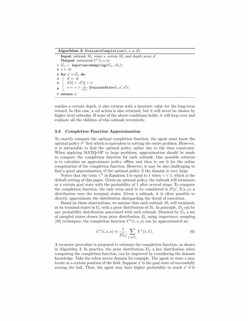
reaches a certain depth, it also returns with a heuristic value for the long-termreward. In this case, a nil action is also returned, but it will never be chosen byhigher level subtasks. If none of the above conditions holds, it will loop over andevaluate all the children of this subtask recursively.

3.3 Completion Function Approximation

To exactly compute the optimal completion function, the agent must know theoptimal policy π∗ first which is equivalent to solving the entire problem. However,it is intractable to find the optimal policy online due to the time constraint.When applying MAXQ-OP to large problems, approximation should be madeto compute the completion function for each subtask. One possible solutionis to calculate an approximate policy offline and then to use it for the onlinecomputation of the completion function. However, it may be also challenging tofind a good approximation of the optimal policy if the domain is very large.

Notice that the term γN in Equation 3 is equal to 1 when γ = 1, which is thedefault setting of this paper. Given an optimal policy, the subtask will terminateat a certain goal state with the probability of 1 after several steps. To computethe completion function, the only term need to be considered is P (s′, N |s, a)–adistribution over the terminal states. Given a subtask, it is often possible todirectly approximate the distribution disregarding the detail of execution.

Based on these observations, we assume that each subtask Mi will terminateat its terminal states in Gi with a prior distribution of Di. In principle, Di can beany probability distribution associated with each subtask. Denoted by G̃a a setof sampled states drawn from prior distribution Da using importance sampling[10] techniques, the completion function C∗(i, s, a) can be approximated as:

C∗(i, s, a) ≈ 1

|G̃a|

∑s′∈G̃a

V ∗(i, s′). (6)

A recursive procedure is proposed to estimate the completion function, as shownin Algorithm 3. In practice, the prior distribution Da–a key distribution whencomputing the completion function, can be improved by considering the domainknowledge. Take the robot soccer domain for example. The agent at state s maylocate in a certain position of the field. Suppose s′ is the goal state of successfullyscoring the ball. Then, the agent may have higher probability to reach s′ if it

directly dribbles the ball to the goal or passes the ball to some teammates whois near the goal, which is specified by the action a in the model.

3.4 Heuristic Search in Action Space

For some domains with large action space, it may be very time-consuming toenumerate all possible actions exhaustively. Hence it is necessary to introducesome heuristic techniques (including prune strategies) to speed up the searchprocess. Intuitively, there is no need to evaluate those actions that are not likelyto be better. In MAXQ-OP, this is done by implementing a iterative version ofSubtasks function which dynamically selects the most promising action to beevaluated next with the tradeoff between exploitation and exploration. Differentheuristic techniques can be used for different subtasks, such as A∗, hill-climbing,gradient ascent, etc. The discussion of the heuristic techniques is beyond thescope of this paper, and the space lacks for a detailed description of it.

4 Implementation in RoboCup 2D

It is our long-term effort to apply the MAXQ-OP framework to the RoboCup 2Ddomain. In this section, we present the implementation details of the MAXQ-OPframework in WrightEagle.

4.1 RoboCup 2D as an MDP

In this section, we present the technical details on modeling the RoboCup 2Ddomain as an MDP. As mentioned, it is a partially-observable multi-agent do-main with continuous state and action space. To model it as a fully-observablesingle-agent MDP, we specify the state and action spaces and the transition andreward functions as follows:

State Space We treat teammates and opponents as part of the environmentand try to estimate the current state with sequences of observations. Then, thestate of the 2D domain can be represented as a fixed-length vector, containingstate variables that totally cover 23 distinct objects (10 teammates, 11 oppo-nents, the ball, and the agent itself).

Action Space All primitive actions, like dash, kick, tackle, turn and turn neck,are originally defined by the 2D domain. They all have continuous parameters,resulting a continuous action space.

Transition Function Considering the fact that autonomous teammates andopponents make the environment unpredictable, the transition function is notobvious to represent. In our team, the agent assumes that all other players sharea same predefined behavior model: they will execute a random kick if the ballis kickable for them, or a random walk otherwise. For primitive actions, theunderlying transition model for each atomic command is fully determined bythe server as a set of generative models.

Reward Function The underlying reward function has a sparse property:the agent usually earns zero rewards for thousands of steps before ball scored orconceded, may causing that the forward search process often terminate without

Fig. 1. MAXQ task graph for WrightEagle

any rewards obtained, and thus can not tell the differences between subtasks. Inour team, to emphasize each subtask’s characteristic and to guarantee that posi-tive results can be found by the search process, a set of pseudo-reward functionsis developed for each subtask.

To estimate the size of the state space, we ignore some secondary variablesfor simplification (such as heterogeneous parameters and stamina information).Totally 4 variables are needed to represent the ball’s state including position(x, y) and velocity (vx, vy). In addition with (x, y) and (vx, vy), two more vari-ables are used to represent each player’s state including body direction db, andneck direction dn. Therefore the full state vector has a dimensionality of 136.All these state variables have continuous values, resulting a high-dimensionalcontinuous state space. If we discretize each state variable into 103 uniformlydistributed values in its own field of definitions, then we obtain a simplifiedstate space with 10408 states, which is extremely larger than domains usuallystudied in the literature.

4.2 Solution with MAXQ-OP

In this section, we describe how to apply MAXQ-OP to the RoboCup soccersimulation domain. Firstly, a series of subtasks at different levels are defined asthe building blocks of constructing the MAXQ hierarchy, listed as follows:– kick, turn, dash, and tackle: They are low-level parameterized primitive ac-

tions originally defined by the soccer server. A reward of -1 is assigned toeach primitive action to guarantee that the optimal policy will try to reacha goal as fast as possible.

– KickTo, TackleTo, and NavTo: In the KickTo and TackleTo subtask, the goalis to kick or tackle the ball to a given direction with a specified velocity,while the goal of the NavTo subtask is to move the agent from its currentlocation to a target location.

– Shoot, Dribble, Pass, Position, Intercept, Block, Trap, Mark, and Formation:These subtasks are high-level behaviors in our team where: 1) Shoot is tokick out the ball to score; 2) Dribble is to dribble the ball in an appropriatedirection; 3) Pass is to pass the ball to a proper teammate; 4) Position is tomaintain the teammate formation for attacking; 5) Intercept is to get the ballas fast as possible; 6) Block is to block the opponent who controls the ball;7) Trap is to hassle the ball controller and wait to steal the ball; 8) Mark is tomark related opponents; 9) Formation is to maintain formation for defense.

– Attack and Defense: Obviously, the goal of Attack is to attack opponents toscore while the goal of Defense is to defense against opponents.

– Root: This is the root task. It firstly evaluate the Attack subtask to seewhether it is ready to attack, otherwise it will try the Defense subtask.The graphical representation of the MAXQ hierarchical structure is shown

in Figure 1, where a parenthesis after a subtask’s name indicates this subtaskwill take parameters. It is worth noting that state abstractions are implicitlyintroduced by this hierarchy. For example in the NavTo subtask, only the agent’sown state variables are relevant. It is irrelevant for the KickTo and TackleTosubtasks to consider those state variables describing other players’ states. Todeal with the large action space, heuristic methods are critical when applyingMAXQ-OP. There are many possible candidates depending on the characteristicof subtasks. For instance, hill-climbing is used when searching over the actionspace of KickTo for the Pass subtask and A* search is used when searching overthe action space of dash and turn for the NavTo subtask.

As mentioned earlier, the method for approximating the completion functionis crucial for the performance when implementing MAXQ-OP. In RoboCup 2D,it is more challenging to compute the distribution because: 1) the forward searchprocess is unable to run into an sufficient depth due to the online time constraint;and 2) the future states are difficult to predict due to the uncertainty of the en-vironment, especially the unknown behaviors of the opponent team. To estimatethe distribution of reaching a goal, we used a variety techniques for differentsubtasks based on the domain knowledge. Take the Attack subtask for example.A so-called impelling speed is used to approximate the completion probability.It is formally defined as:

impelling speed(s, s′, α) =dist(s, s′, α) + pre dist(s′, α)

step(s, s′) + pre step(s′), (7)

where α is a given direction (called aim-angle), dist(s, s′, α) is the ball’s runningdistance in direction α from state s to state s′, step(s, s′) is the estimated stepsfrom state s to state s′, pre dist(s′) estimates final distance in direction α thatthe ball can be impelled forward starting from state s′, and pre step(s′) esti-mates the respective steps. The aim-angle in state s is determined dynamicallyby aim angle(s) function. The value of impelling speed(s, s′, aim angle(s)) in-dicates the fact that the faster the ball is moved in a right direction, the moreattack chance there would be. In practice, it makes the team attack more effi-cient. As a result, it can make a fast score within tens of steps in the beginningof a match. Different definitions of the aim angle function can produce substan-tially different attack styles, leading to a very flexible and adaptive strategy,particularly for unfamiliar teams.

5 Empirical Evaluation

To test how the MAXQ-OP framework affects our team’s final performance, wecompared three different versions of our team, including:– Full: This is exactly the full version of our team, where a complete MAXQ-

OP online planning framework is implemented as the key component.

Fig. 2. A selected scene from the final match of RoboCup 2011

– Random: This is nearly the same as Full, except that when the ball iskickable for the agent and the Shoot behavior finds no solution, the Attackbehavior randomly chooses a macro-action to perform between Pass andDribble with uniform probability.

– Hand-coded: This is similar to Random, but instead of a random selectionbetween Pass and Dribble, a hand-coded strategy is used. With this strategy,if there is no opponent within 3m from the agent, then Dribble is chosen;otherwise, Pass is chosen.

The only difference between Full, Random and Hand-coded is the local se-lection strategy between Pass and Dribble in the Attack behavior. In Full, thisselection is automatically based on the value function of subtasks (i.e. the so-lutions found by EvaluateState(Pass, ·, ·) and EvaluateState(Dribble, ·, ·) inthe MAXQ-OP framework). Although Random and Hand-coded have dif-ferent Pass-Dribble selection strategies, the other subtasks of Attack, includingShoot, Pass, Dribble, and Intercept, as that of Full, remain the same.

For each version, we use an offline coach (also known as a trainer) to inde-pendently run the team against the Helios11 binary (which has participated inRoboCup 2011 and won the second place) for 100 episodes. Each episode beginswith a fixed scene (i.e. the full state vector) taken from the final match we haveparticipated in of RoboCup 2011, and ends when: 1) our team scores a goal, de-noted by success; or 2) the ball’s x coordination is smaller than -10, denoted byfailure; or 3) the episode lasts longer than 200 cycles, denoted by timeout. Itis worth mentioning that although all of the episode begin with the same scene,none of them is identical due to the uncertainty of the environment.

The selected scene, which is originally located at cycle #3142 of that match, isdepicted in Figure 2 where white circles represent our players, gray ones representopponents, and the small black one represents the ball. We can see that our player10 was holding the ball at that moment, while 9 opponents (including goalie)were blocking just in front of their goal area. In RoboCup 2011, teammate 10passed the ball directly to teammate 11. Having got the ball, teammate 11decided to pass the ball back to teammate 10. When teammate 11 had movedto an appropriate position, the ball was passed again to it. Finally, teammate11 executed a tackle to shoot at cycle #3158 and scored a goal 5 cycles later.

Table 1 summarizes the test results showing that the Full version of ourteam outperforms both Random and Hand-coded with an increase of the

Table 1. Empirical results of WrightEagle in episodic scene test

Version Episodes Success Failure Timeout

Full 100 28 31 41Random 100 15 44 41

Hand-coded 100 17 38 45

Table 2. Empirical results of WrightEagle in full game test

Opponent Team Games Avg. Goals Avg. Points Winning Rate

BrainsStomers08 100 3.09 : 0.82 2.59 : 0.28 82.0± 7.5%Helios10 100 4.30 : 0.88 2.84 : 0.11 93.0± 5.0%Helios11 100 3.04 : 1.33 2.33 : 0.52 72.0± 8.8%Oxsy11 100 4.97 : 1.33 2.79 : 0.16 91.0± 5.6%

chance of sucess by 86.7% and 64.7% respectively. We find that although Full,Random and Hand-coded have the same hierarchical structure and subtasksof Attack, the local selection strategy between Pass and Dribble plays a key rolein the decision of Attack and affects the final performance substantially. It can beseen from the table that MAXQ-OP based local selection strategy between Passand Dribble is sufficient for the Attack behavior to achieve a high performance.Recursively, this is also true for other subtasks over the MAXQ hierarchy, suchas Defense, Shoot, Pass, etc. To conclude, MAXQ-OP is able to be the key tosuccess of our team in this episodic scene test.

We also tested the Full version of our team in full games against 4 bestRoboCup 2D opponent teams, namely BrainsStomers08, Helios10, Helios11 andOxsy11, where BrainStormers08 and Helios10 were the champion of RoboCup2008 and RoboCup 2010 respectively. In the experiments, we independently ranour team against the binary codes officially released by them for 100 games onexactly the same hardware. Table 2 summarizes the detailed empirical resultswith our winning rate, which is defined as p = n/N , where n is the number ofgames we won, and N is the total number of games. It can be seen from the tablethat our team with the implementation of MAXQ-OP substantially outperformsother tested teams. Specifically, our team had about 82.0%, 93.0%, 72.0% and91.0% of the chances to win BrainsStomers08, Helios10, Helios11 and Oxsy11respectively.

While there are multiple factors contributing to the general performance of aRoboCup 2D team, it is our observation that our team benefits greatly from theabstraction we made for the actions and states. The key advantage of MAXQ-OPin our team is to provide a formal framework for conducting the search processover a task hierarchy. Therefore, the team can search for a strategy-level solutionautomatically online by given the pre-defined task hierarchy. To the best of ourknowledge, most of the current RoboCup teams develop their team based onhand-coded rules and behaviors.

6 Conclusions

This paper presents a novel approach to automated planning in the RoboCup 2Ddomain. It benefits from both the advantage of hierarchical decomposition andthe power of heuristics. Barry et al. proposed an offline algorithm called DetH*[3] to solve large MDPs hierarchically by assuming that the transitions betweenmacro-states are totally deterministic. In contrast, we assume a prior distributionover the terminal states of each subtask, which is more realistic. The MAXQ-OP framework has been implemented in the team WrightEagle. The empiricalresults indicated that the agents developed with this framework and the relatedtechniques reached outstanding performances, showing its potential of scalabilityto very large domains. This demonstrates the soundness and stability of MAXQ-OP for solving large MDPs with the pre-defined task hierarchy. In the future,we plan to theoretically analyze MAXQ-OP with different task priors and try togenerate these priors automatically.

7 Acknowledgments

This work is supported by the National Hi-Tech Project of China under grant2008AA01Z150 and the Natural Science Foundation of China under grant 60745002and 61175057. The authors thank Haochong Zhang, Guanghui Lu, and MiaoJiang for their contributions to this work. We are also grateful to the anony-mous reviewers for their constructive comments and suggestions.

References

1. Bai, A., Wu, F., Chen, X.: Online planning for large MDPs with MAXQ decom-position (extended abstract). In: Proc. of 11th Int. Conf. on Autonomous Agentsand Multiagent Systems. Valencia, Spain (June 2012)

2. Barry, J.: Fast Approximate Hierarchical Solution of MDPs. Ph.D. thesis, Mas-sachusetts Institute of Technology (2009)

3. Barry, J., Kaelbling, L., Lozano-Perez, T.: Deth*: Approximate hierarchical so-lution of large markov decision processes. In: International Joint Conference onArtificial Intelligence. pp. 1928–1935 (2011)

4. Dietterich, T.G.: Hierarchical reinforcement learning with the MAXQ value func-tion decomposition. Journal of Machine Learning Research 13(1), 63 (May 1999)

5. Gabel, T., Riedmiller, M.: On progress in robocup: the simulation league showcase.RoboCup 2010: Robot Soccer World Cup XIV pp. 36–47 (2011)

6. Kalyanakrishnan, S., Liu, Y., Stone, P.: Half field offense in robocup soccer: Amultiagent reinforcement learning case study. RoboCup 2006: Robot Soccer WorldCup X pp. 72–85 (2007)

7. Riedmiller, M., Gabel, T., Hafner, R., Lange, S.: Reinforcement learning for robotsoccer. Autonomous Robots 27(1), 55–73 (2009)

8. Stone, P.: Layered learning in multiagent systems: A winning approach to roboticsoccer. The MIT press (2000)

9. Stone, P., Sutton, R., Kuhlmann, G.: Reinforcement learning for robocup soccerkeepaway. Adaptive Behavior 13(3), 165–188 (2005)

10. Thrun, S., Fox, D., Burgard, W., Dellaert, F.: Robust monte carlo localization formobile robots. Artificial intelligence 128(1-2), 99–141 (2001)