Toward Sustainable Electronic Beehive Monitoring ... · Abstract—Two algorithms are presented for...

Abstract—Two algorithms are presented for omnidirectional

bee counting from images to estimate forager traffic levels. An

audio processing algorithm is also presented for digitizing bee

buzzing signals with harmonic intervals into A440 piano note

sequences. The three algorithms were tested on samples

collected through four beehive monitoring devices deployed at

different apiaries in Northern Utah over extended periods of

time. On a sample of 378 images from a deployed beehive

monitoring device, the first algorithm for omnidirectional bee

counting achieved an accuracy of 73 percent. The second

algorithm for omnidirectional bee counting achieved an

accuracy of 80.5 percent on a sample of 1005 images with green

pads and an accuracy of 85.5 percent on a sample of 776

images with white pads. The note range detected by the

proposed audio processing algorithm on a sample of 3421.52

MB of wav data contained the first four octaves, with the

lowest note being A0 and the highest note being F#4.

Experimental results indicate that computer vision and audio

analysis will play increasingly more significant roles in

sustainable electronic beehive monitoring devices used by

professional and amateur apiarists.

Index Terms—computer vision; audio analysis, electronic

beehive monitoring, sustainable computing

I. INTRODUCTION

ince 2006 honeybees have been disappearing from many

amateur and commercial apiaries. This trend has been

called the colony collapse disorder (CCD) [1]. The high

rates of colony loss threaten to disrupt the world’s food

supply. A consensus is emerging among researchers and

practitioners that electronic beehive monitoring (EBM) can

help extract critical information on colony behavior and

phenology without invasive beehive inspections [2].

Continuous advances in electronic sensor and solar

harvesting technologies make it possible to transform

apiaries into ad hoc sensor networks that collect multi-

sensor data to recognize bee behavior patterns.

In this article, two algorithms are presented for

omnidirectional bee counting from images to estimate

Manuscript received July 2, 2016.

Vladimir. A. Kulyukin is with the Department of Computer Science of

Utah State University, Logan, UT 84322 USA (phone: 434-797-2451; fax:

435-791-3265; e-mail: [email protected]).

Sai Kiran Reka is with the Department of Computer Science of Utah

State University, Logan, UT USA 84322.

forager traffic levels. An audio processing algorithm is also

presented for digitizing bee buzzing signals with harmonic

intervals into A440 piano note sequences. The three

algorithms were tested on samples collected through four

beehive monitoring devices deployed at different apiaries in

Northern Utah over extended periods of time. When viewed

as time series, forager traffic estimates and note sequences

can be correlated with other timestamped data for pattern

recognition. It is probable that other musical instruments can

be used for obtaining note sequences so long as their notes

have standard frequencies detectable in a numerically stable

manner.

The standard modern piano keyboard is called the A440

88-keyboard, because it has eighty-eight keys where the

fifth A, called A4, is tuned to a frequency of 440 Hz [3].

The standard list of frequencies for an ideally tuned piano is

used for tuning actual instruments. For example, A#4, the

50-th key on the 88-key keyboard has a frequency of 466.14

Hz. In this article, the terms note and key are used

interchangeably.

Buzzing signals and images are captured by a solar-

powered, electronic beehive monitoring device (EBMD),

called BeePi. BeePi is designed for the Langstroth hive [4]

used by many beekeepers worldwide. Four BeePi EBMDs

were assembled and deployed at two Northern Utah apiaries

to collect 28 gigabytes of audio, temperature, and image

data in different weather conditions. Except for drilling

narrow holes in inner hive covers for temperature sensor

and microphone wires, no structural hive modifications are

required for deployment.

The remainder of this article is organized as follows. In

Section II, related work is reviewed. In Section III, the

hardware and software details of BeePi are presented and

collected data are described. In Section IV, the first

algorithm is presented for omnidirectional bee counting on

Langstroth hive landing pads. In Section V, the second

algorithm is presented for omnidirectional bee counting on

Langstroth hive landing pads. In Section VI, an audio

processing algorithm is proposed for digitizing buzzing

signals into A440 piano note sequences by using harmonic

intervals. In Section VII, an audio data analysis is presented.

In Section VIII, conclusions are drawn.

II. RELATED WORK

Beehives of all sorts and shapes have been monitored by

Toward Sustainable Electronic Beehive

Monitoring: Algorithms for Omnidirectional

Bee Counting from Images and Harmonic

Analysis of Buzzing Signals

Vladimir A. Kulyukin and Sai Kiran Reka

S

Engineering Letters, 24:3, EL_24_3_12

(Advance online publication: 27 August 2016)

______________________________________________________________________________________

Fig. 2. Covered BeePi camera.

Fig. 3. Solar panels on beehives.

humans for centuries. Gates collected hourly temperature

measurements from a Langstroth beehive in 1914 [5]. In the

1950’s, Woods placed a microphone in a beehive [6] and

identified a warbling noise in the range from 225 to 285 Hz.

Woods subsequently built Apidictor, an audio beehive

monitoring tool. Bencsik [7] equipped several hives with

accelerometers and observed increasing amplitudes a few

days before swarming, with a sharp change at the point of

swarming. Evans [8] designed Arnia, a beehive monitoring

system that uses weight, temperature, humidity, and sound.

The system breaks down hive sounds into flight buzzing,

fanning, and ventilating and sends SMS or email alerts to

beekeepers.

Several EBM projects have focused on swarm detection.

S. Ferrari et al. [9] assembled an ad hoc system for

monitoring swarm sounds in beehives. The system consisted

of a microphone, a temperature sensor, and a humidity

sensor placed in a beehive and connected to a computer in a

nearby barn via underground cables. The sounds were

recorded at a sample rate of 2 kHz and analyzed with

MATLAB and Cool Edit Pro. The researchers monitored

three beehives for 270 hours and observed that swarming

was indicated by an increase of the buzzing frequency at

about 110 Hz with a peak at 300 Hz when the swarm left the

hive. Another finding was that a swarming period correlated

with a rise in temperature from 33° C to 35° C with a

temperature drop to 32° C at the actual time of swarming.

Rangel and Seeley [10] investigated signals of honeybee

swarms. Five custom designed observation hives were

sealed with glass covers. The captured video and audio data

were monitored daily by human observers. The researchers

found that approximately one hour before swarm exodus,

the production of piping signals gradually increased and

ultimately peaked at the start of the swarm departure.

Meikle and Holst [11] placed four beehives on precision

electronic scales linked to data loggers to record weight for

over sixteen months. The researchers investigated the effect

of swarming on daily data and reported that empty beehives

had detectable daily weight changes due to moisture level

changes in the wood.

Bromenshenk et al. [12] designed and deployed bi-

directional, IR bee counters in their multi-sensor

SmartHive® system. The researchers found their IR

counters to be more robust and accurate than capacitance

and video-based systems. Since the IR counters required

regular cleaning and maintenance, a self-diagnostic program

was developed to check whether all of the emitters and

detectors were functioning properly and the bee portals were

not blocked by debris or bees.

III. SOLAR-POWERED ELECTRONIC BEEHIVE MONITORING

A. Hardware

A fundamental objective of the BeePi design is

reproducibility: other researchers and practitioners should

be able to replicate our results at minimum cost and time

commitments. Each BeePi consists of a raspberry pi

computer, a miniature camera, a solar panel, a temperature

sensor, a battery, a hardware clock, and a solar charge

controller.

The exact BeePi hardware components are shown in Fig.

1. We used the Pi Model B+ 512MB RAM models, Pi T-

Cobblers, half-size breadboards, waterproof DS18B20

digital temperature sensors, and Pi cameras (see Fig. 2). For

solar harvesting, we used the Renogy 50 watts 12 Volts

monocrystalline solar panels, Renogy 10 Amp PWM solar

charge controllers, Renogy 10ft 10AWG solar adaptor kits,

and the UPG 12V 12Ah F2 sealed lead acid AGM deep-

cycle rechargeable batteries. All hardware fits in a shallow

super, except for the solar panel that is placed on top of a

hive (see Fig. 3) or next to it (see Fig. 4).

Fig. 1. BeePi hardware components.

Two holes were drilled in the inner hive cover under a

super with the BeePi hardware for a temperature sensor and

a microphone. The temperature sensor chord was lowered

into the second deep super (the first deep super is the lowest

one) with nine frames of live bees to the left of frame 1. The



______________________________________________________________________________________

Fig. 4. BeePi in an overwintering beehive.

microphone chord was lowered into the second deep super

to the right of frame 9. More holes can be drilled if the

placements of the microphone and temperature sensors

should be changed.

The camera is placed outside to take static snapshots of

the beehive’s entrance, as shown in Fig. 2. A small piece of

hard plastic was placed above the camera to protect it from

the elements. Fig. 3 displays the solar panels on top of two

hives equipped with BeePi devices at the Utah State

University Organic Farm. The solar panels were tied to the

hive supers with bungee cords. It takes approximately 20

minutes to wire a BeePi monitor for deployment. Fig. 5

shows the first author wiring two such monitors at an apiary

in spring 2016.

Fig. 5. Wiring BeePi monitors for deployment .

B. Software

In each BeePi, all data collection is done on the raspberry

pi computer. The collected data is saved on a 25G sdcard

inserted into the pi. Data collection software is written in

Python 2.7. When the system starts, three data collection

threads are spawned. The first thread collects temperature

readings every 10 minutes and saves them into a text file.

The second thread collects 30-second wav recordings every

15 minutes. The third thread saves PNG pictures of the

beehive’s landing pad every 15 minutes.

A cronjob monitors the threads and restarts them after

hardware failures. For example, during a field deployment

the camera of one of the EBMDs stopped functioning due to

excessive heat. The cronjob would periodically restart the

PNG thread until the temperature went down and the camera

started functioning properly again.

C. Field Deployment

Three field deployments of BeePi devices have been

executed so far. The first deployment was on private

property in Logan, UT in early fall 2014. A BeePi was

placed into an empty hive and ran exclusively on solar

power for two weeks.

The second deployment was in Garland, UT in December

2014 – January 2015 in subzero temperatures. A BeePi in a

hive with overwintering bees is shown in Fig. 4. Due to

strong winter winds typical for Northern Utah, the solar

panel was placed next to the hive on an empty super and

tied down to a hive stand with bungee cords to ensure its

safety. The BeePi successfully operated for nine out of the

fourteen days of deployment exclusively on solar power.

Over 3 gigabytes of pictures, wav files, and temperature

readings were obtained during the nine operational days.

These field deployments indicate that electronic beehive

monitoring may be sustained by solar power.

IV. OMNIDIRECTIONAL BEE COUNTING: ALGORITHM 1

Visual estimates of forager traffic are used by professional

and amateur beekeepers to evaluate the health of a bee

colony. In electronic beehive monitoring, computer vision

can be used to estimate the amount of forager traffic from

captured images. A sample image is shown in Fig. 6.

Fig. 6. Image captured from the BeePi camera.

The vision-based bee counting algorithms presented in

this section and in Section V are omnidirectional, because

they do not distinguish incoming and outgoing bee traffic.

The reason why no directionality is integrated is two-fold.

First, a robust vision-based solution to directionality will

likely require video processing. Since the BeePi relies

exclusively on solar power, in situ video capture and storage

will drain the battery faster, thereby making EBM more

disruptive. Second, omnidirectional bee counting can still be

used as a valuable estimate of forager traffic so long as it

accurately counts bees on landing pads. All algorithms were

implemented in Java using the OpenCV 2 image processing

library (www.opencv.org).

Since the camera’s position is fixed, there is no need to

process the entire image. The image processing starts by

cropping a rectangular region of interest (ROI) where the

landing pad is likely to be. The ROI is made wider and

longer than the landing pad, because the camera may

occasionally swing up, down and sideways in stronger



______________________________________________________________________________________

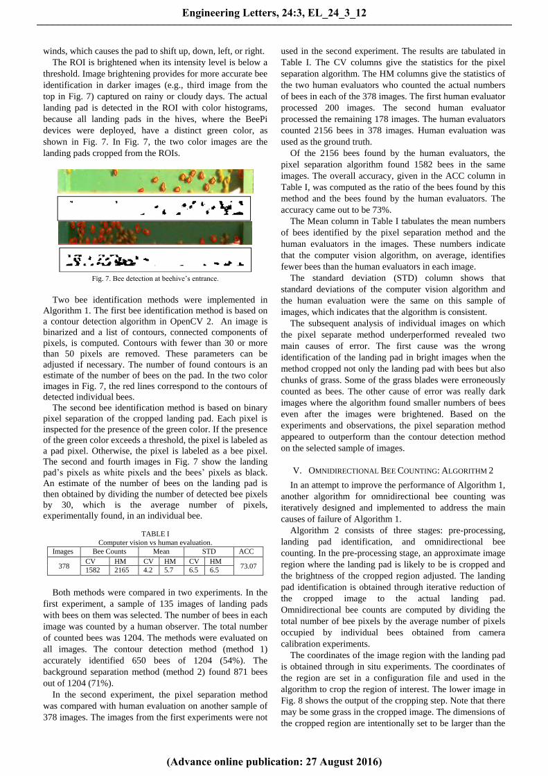
winds, which causes the pad to shift up, down, left, or right.

The ROI is brightened when its intensity level is below a

threshold. Image brightening provides for more accurate bee

identification in darker images (e.g., third image from the

top in Fig. 7) captured on rainy or cloudy days. The actual

landing pad is detected in the ROI with color histograms,

because all landing pads in the hives, where the BeePi

devices were deployed, have a distinct green color, as

shown in Fig. 7. In Fig. 7, the two color images are the

landing pads cropped from the ROIs.

Fig. 7. Bee detection at beehive’s entrance.

Two bee identification methods were implemented in

Algorithm 1. The first bee identification method is based on

a contour detection algorithm in OpenCV 2. An image is

binarized and a list of contours, connected components of

pixels, is computed. Contours with fewer than 30 or more

than 50 pixels are removed. These parameters can be

adjusted if necessary. The number of found contours is an

estimate of the number of bees on the pad. In the two color

images in Fig. 7, the red lines correspond to the contours of

detected individual bees.

The second bee identification method is based on binary

pixel separation of the cropped landing pad. Each pixel is

inspected for the presence of the green color. If the presence

of the green color exceeds a threshold, the pixel is labeled as

a pad pixel. Otherwise, the pixel is labeled as a bee pixel.

The second and fourth images in Fig. 7 show the landing

pad’s pixels as white pixels and the bees’ pixels as black.

An estimate of the number of bees on the landing pad is

then obtained by dividing the number of detected bee pixels

by 30, which is the average number of pixels,

experimentally found, in an individual bee.

TABLE I

Computer vision vs human evaluation.

Images Bee Counts Mean STD ACC

378 CV HM CV HM CV HM

73.07 1582 2165 4.2 5.7 6.5 6.5

Both methods were compared in two experiments. In the

first experiment, a sample of 135 images of landing pads

with bees on them was selected. The number of bees in each

image was counted by a human observer. The total number

of counted bees was 1204. The methods were evaluated on

all images. The contour detection method (method 1)

accurately identified 650 bees of 1204 (54%). The

background separation method (method 2) found 871 bees

out of 1204 (71%).

In the second experiment, the pixel separation method

was compared with human evaluation on another sample of

378 images. The images from the first experiments were not

used in the second experiment. The results are tabulated in

Table I. The CV columns give the statistics for the pixel

separation algorithm. The HM columns give the statistics of

the two human evaluators who counted the actual numbers

of bees in each of the 378 images. The first human evaluator

processed 200 images. The second human evaluator

processed the remaining 178 images. The human evaluators

counted 2156 bees in 378 images. Human evaluation was

used as the ground truth.

Of the 2156 bees found by the human evaluators, the

pixel separation algorithm found 1582 bees in the same

images. The overall accuracy, given in the ACC column in

Table I, was computed as the ratio of the bees found by this

method and the bees found by the human evaluators. The

accuracy came out to be 73%.

The Mean column in Table I tabulates the mean numbers

of bees identified by the pixel separation method and the

human evaluators in the images. These numbers indicate

that the computer vision algorithm, on average, identifies

fewer bees than the human evaluators in each image.

The standard deviation (STD) column shows that

standard deviations of the computer vision algorithm and

the human evaluation were the same on this sample of

images, which indicates that the algorithm is consistent.

The subsequent analysis of individual images on which

the pixel separate method underperformed revealed two

main causes of error. The first cause was the wrong

identification of the landing pad in bright images when the

method cropped not only the landing pad with bees but also

chunks of grass. Some of the grass blades were erroneously

counted as bees. The other cause of error was really dark

images where the algorithm found smaller numbers of bees

even after the images were brightened. Based on the

experiments and observations, the pixel separation method

appeared to outperform than the contour detection method

on the selected sample of images.

V. OMNIDIRECTIONAL BEE COUNTING: ALGORITHM 2

In an attempt to improve the performance of Algorithm 1,

another algorithm for omnidirectional bee counting was

iteratively designed and implemented to address the main

causes of failure of Algorithm 1.

Algorithm 2 consists of three stages: pre-processing,

landing pad identification, and omnidirectional bee

counting. In the pre-processing stage, an approximate image

region where the landing pad is likely to be is cropped and

the brightness of the cropped region adjusted. The landing

pad identification is obtained through iterative reduction of

the cropped image to the actual landing pad.

Omnidirectional bee counts are computed by dividing the

total number of bee pixels by the average number of pixels

occupied by individual bees obtained from camera

calibration experiments.

The coordinates of the image region with the landing pad

is obtained through in situ experiments. The coordinates of

the region are set in a configuration file and used in the

algorithm to crop the region of interest. The lower image in

Fig. 8 shows the output of the cropping step. Note that there

may be some grass in the cropped image. The dimensions of

the cropped region are intentionally set to be larger than the



______________________________________________________________________________________

actual landing pad to compensate for camera swings in

strong winds.

Fig. 8. Cropped landing pad (below) from original image (above).

Image brightness is dependent on the weather. Brightness

is maximal when the sun is directly above the beehive.

However, when the sun is obscured by clouds, captured

images tend to be darker. As experiments with Algorithm 1

described in Section IV showed, both cases had an adverse

effect on bee counting. To minimize this effect, image

brightness is dynamically adjusted to lie in (45, 95), i.e., the

brightness index should be greater than 45 but less than 95.

This range was experimentally found to yield optimal

results.

Fig. 9 illustrates how brightness adjustment improves

omnidirectional bee counts. The upper image on the right in

Fig. 9 shows a green landing pad extracted from the cropped

image on the left without adjusted brightness. The lower

image on the right in Fig. 9 shows a green pad extracted

from the same image with adjusted brightness. Only four

bees were identified in the upper image on the left whereas

in the lower image eight bees were identified, which is

closer to the twelve bees found in the original image by

human counters.

Fig. 9. Extraction of green pad with from image with adjusted brightness.

The three steps of the landing pad identification in the

cropped region, i.e., the output of the pre-processing stage,

are shown in Fig. 10. The first step in identifying the actual

landing pad in the approximate region cropped in the pre-

processing stage is to convert the pre-processed RGB image

to the Hue Saturation Value (HSV) format, where H and S

values are computed with Equation (1).

(1)

In (1), are the R, G, B values normalized by 255,

and

The value of V is set to . In the actual implementation,

the format conversion is accomplished with the cvtColor()

method of OpenCV. The inRange() method of OpenCV is

subsequently applied to identify the areas of green or white

pixels, the two colors in which the landing pads of our

beehives are painted.

Noise is removed through a series of erosions and

dilations. The white pixels in the output image represent

green or white color in the actual image and the black pixels

represent any color other than green or white.

Fig. 10. Landing pad identification steps: 1) HSV conversion; 2) color

range identification; 3) noise removal.

To further remove noise from the image and reduce it as

closely as possible to the actual landing pad, contours are

computed with the findContours() method of OpenCV and a

bounding rectangle is found for each contour. The bounding

contour rectangles are sorted in increasing order by the Y

coordinate, i.e., increasing rows. Thus, the contours in the

first row of the image will be at the start of the list. Fig. 11

shows the bounding rectangles for the contours computed

for the output image of step 3 in Fig. 10.

Fig. 11. Bounding rectangles of found contours.

Data analysis indicates that if the area of a contour is at

least half the estimated area of the landing pad, the contour

is likely to be part of the actual landing pad. On the other

hand, if the area of a contour is less than 20 pixels, that

contour is likely to be noise and should be discarded.

In the current implementation of the algorithm, the

estimated area of the green landing pad is set to 9000 pixels

and the estimated area of the white landing pad is set to

12000 pixels. These parameters can be adjusted for distance.

Using the above pixel area size filter, the approximate

location of the landing pad is computed by scanning through

all the contours in the sorted list and finding the area of each



______________________________________________________________________________________

contour. If the area is at least half the estimated size of the

landing pad of the appropriate color, the Y coordinate of the

contour rectangle is taken to be the average Y coordinate

and the scanning process terminates.

If the contour’s area is between 20 and half the estimated

landing pad area, the Y coordinate of the contour is saved.

Otherwise, the current contour is skipped and the next

contour is processed. When the first contour scan

terminates, the average Y coordinate, μ(Y), is calculated by

dividing the sum of the saved Y coordinates by the number

of the processed contour rectangles.

After μ(Y) is computed, a second scan of the sorted

contour rectangle list is performed to find all contours

whose height lies in [μ(Y)-H, μ(Y)+H], where H is half of

the estimated height of the landing pad for the appropriate

color.

While the parameter H may differ from one beehive to

another, as the alignment of the camera differs from one

hive to another, it can be experimentally found for each

beehive. For example, if the camera is placed closer to the

landing pad, then H will have a higher value and if the

camera is placed far from the landing pad, H will have a

lower value. In our case, H was set to 20 for green landing

pad images and to 25 and for white landing pad images.

Bounding rectangles are computed after the second scan

to enclose all points in the found contours, as shown in Fig.

12. To verify whether the correct landing pad area has been

identified, the area of the bounding rectangle is computed.

If the area of the bounding rectangle is greater than the

estimated area of the landing pad, the bounding rectangle

may contain noise, in which case another scan is iteratively

performed to remove noise by decreasing H by a small

amount of 2 to 4 units. In most of the cases, this extra scan

is not needed, because the landing pad is accurately found.

Fig. 12 illustrates the three steps of the contour analysis to

identify the actual landing pad.

Fig. 12. Contour analysis: 1) 1st contour scan; 2) 2nd contour scan; 3) pad

cropping.

Foreground and background pixels are separated on color.

Specifically, in the current implementation of the algorithm,

for green landing pads, the background is assumed to be

green and the foreground, i.e., the bees, is assumed to be

yellow; for white landing pads, the background is assumed

to be white and the foreground is assumed to be yellow.

All pixels with shades of green or white are set to 255 and

the remaining pixels are set to 0. Three rows of border

pixels of the landing pad image are arbitrarily set to 255 to

facilitate bee identification in the next step. Fig. 13 shows

the output of this stage. In Fig. 13, the green background is

converted to white and the foreground to black. Since noise

may be introduced, the image is de-noised through a series

of erosions and dilation with a 2 x 2 structuring element.

Fig. 13. Background and foreground separation.

To identify bees in the image, the image from the

previous stage is converted to grayscale and the contours are

computed again. Data analysis suggests that the area of an

individual bee or a group of bees vary from 20 to 3000

pixels. Therefore, if the area of a contour is less than 20

pixels or greater than 3000 pixels, the contour is removed.

The area of one individual bee is between 35 and 100

pixels, depending on the distance of the pi camera from the

landing pad. The green landing pad images were captured

by a pi camera placed approximately 1.5m above the

landing pad with the average area of the bee being 40

pixels.

On the other hand, the white landing pad images were

captured by a pi camera placed approximately 70cm above

the landing pad where the average area of an individual bee

is 100 pixels. To find the number of bees in green landing

pad images, the number of the foreground pixels, i.e., the

foreground area, is divided by 40 (i.e., the average bee pixel

area on green landing pads), whereas, for the white landing

pad images, the foreground area is divided by 100 (i.e., the

average bee pixel area on white landing pads). The result is

the most probable count of bees in the image. In the upper

image in Fig. 14, five bees are counted by the algorithm.

The lower image in Fig. 14 shows the found bees in the

original image.

Fig. 14. Omnidirectional bee counting.

A sample of 1005 green pad images and 776 white pad

images were taken from the data captured with two BeePi

EBMDs deployed at two Northern Utah apiaries. Each

image has a resolution of 720 x 480 pixels and takes 550KB

of space. To obtain the ground truth, six human evaluators

were recruited. Each evaluator was given a set of images

and asked to count bees in each image and record their

observations in a spread sheet. The six spread sheets were

subsequently combined into a single spread sheet.

Table II gives the ground truth statistics. The human

evaluators identified a total of 5,770 bees with an average of

5.7 bees per image in images with green landing pads. In

images with white landing pads, the evaluators identified a

total of 2,178 bees with a mean of 2.8 bees per image.

Table III summarizes the performance of the algorithm ex

situ on the same green and white pad images. The algorithm

identified 5,263 bees out of 5,770 in the green pad images

with an accuracy of 80.5% and a mean of 5.2 bees per

image. In the white pad images, the algorithm identified

2,226 bees out of 2,178 with an accuracy of 85.5% and an

average of 2.8 bees per image. The standard deviations of

the algorithm were slightly larger than those of the human

evaluators.



______________________________________________________________________________________

TABLE II

Ground truth statistics.

Pad Color Num Images Total Bees Mean STD

Green 1,005 5,770 5.7 6.8

White 776 2,178 2.8 3.4

TABLE III

Ex situ performance of algorithm 2.

Pad Color Num Images Total Bees Mean STD ACC

Green 1,005 5,263 5.2 7.6 80.5

White 776 2,178 2.8 4.1 85.5

Fig. 15. False positives.

Our analysis of the results identified both true negatives

and false positives. There appear to be fewer true negatives

than false positives. The main reason for true negatives is

the algorithm’s conservative landing pad identification,

which causes some actual bees to be removed from the

image.

The bees on the sides of the landing pad are also typically

removed from the image. Another reason for true negatives

is image skewness due to wind induced camera swings. If

the landing pad is skewed, then a part of the landing pad is

typically cropped out during the bounding rectangle

computation. In some images, some actual bees were

removed from images during image de-noising, which

resulted in lower bee counts compared to human counts.

False positives were primarily caused by occasional

shades, leaves, or blades of grass wrongly counted as bees.

Fig. 15 gives an example of false positives. A human

evaluator counted 9 bees in the upper image whereas the

algorithm counted 28 bees on the landing pad (lower image

in Fig. 15) cropped out of the upper image. The shade

pixels on the right end of the cropped landing pad were

counted as bees, which resulted in a much higher bee count

than the human evaluator’s count.

VI. AUDIO ANALYSIS OF BUZZING SIGNALS WITH

HARMONIC INTERVALS

Digitizing buzzing signals into A440 piano note

sequences is a method of obtaining a symbolic

representation of signals grounded in time. When viewed as

a time series, such sequences can be correlated with other

timestamped data such as estimates of forager bee traffic

levels or temperatures.

Bee buzzing audio signals were first processed with the

Fast Fourier Transform (FFT), as implemented in Octave

[11], to compute the FFT frequency spectrograms to identify

the A440 piano key notes. The quality of the computed

spectrograms was inadequate for reliable note identification

due to low volumes.

The second attempt, which also relied on Fourier

analysis, did not use the FFT. A more direct, although less

efficient, method outlined in Tolstov’s monograph [12] was

used. Tolstov’s method relies on periodic functions f(x) with

a period of 2π that have expansions given in (1).

Multiplying both sides of (1), separately, by cos(nx) and by

sin(nx), integrating the products from -π to π, and

regrouping, the equations in (2) are obtained for the Fourier

coefficients in the Fourier series of f(x). The interval of

integration can be defined not only on [-π, π] but also on [a,

a+2π] for some real number a, as in (3).

(1)

(2)

(3)

In many real world audio processing situations, when f(x)

is represented by a finite audio signal, it is unknown

whether the series on the right side of (1) converges and

actually equals the sum of f(x). Therefore, only the

approximate equality in (4) can be used. Tolstov’s method

defines constituent harmonics in f(x) by (5).

(4)

(5)

The proposed algorithm for detecting A440 piano notes

in beehive audio samples is based on Tolstov’s method and

implemented in Java. An A440 key K is represented as a

harmonic defined in (5). Since n in (5) is a non-negative

integer and note frequencies are real numbers, K is defined

in (6) as a set of harmonics where f is K’s A440 frequency

in Hz and b is a small positive integer that defines a band of

integer frequencies centered around K’s real frequency. For

example, the A440 frequency of A0 is 27.56 Hz. Thus, a set

of six integer harmonics, from h25(x) to h30(x), can be

defined to identify the presence of A0 in a signal, as in (7).

The presence of a key in a signal is done by thresholding

the absolute values of the Fourier coefficients or harmonic

magnitudes. Thus, a key is present in a signal if the set in

(6) is not empty for a given value of b and a given

threshold.



______________________________________________________________________________________

(6)

(7)

A Java class in the current implementation of the

algorithm takes wav files and generates LOGO music files

for the LOGO Music Player (LMP)

(www.terrapinlogo.com). Fig. 16 shows several lines from

an LMP file generated from a wav file. PLAY is a LOGO

function. The remainder of each line consists of the

arguments to this function in square brackets. A single pair

of brackets indicates a one-note chord; double brackets

indicate a chord consisting of multiple resulting notes.

Fig. 16. LMP instructions with A440 notes detected in wav files.

Fig. 17. Musical score of bee buzzing.

To visualize beehive music, the audio files generated by

the LMP can be converted into musical scores. Fig. 17 gives

one such score obtained with ScoreCloud Studio

(http://scorecloud.com) from an LMP file converted to midi.

VII. AUDIO DATA ANALYSIS

The audio digitization algorithm described in Section VI

was applied to the buzzing signals collected by a BeePi

device at the USU Organic Farm from 22:00 on July 4th,

2015 to 00:00 on July 7th, 2015.

Each signal was saved as a 30-second wav file. A total of

152 wav files were collected in this period, which amounted

to a total of 3421.52 MB of wav data. The digitization

algorithm described in Section VI was applied to these data

on a PC running Ubuntu 12.04 LTS.

The A440 piano keys were mapped to integers from 1 to

88 so that A0 was mapped to 1 and C8 to 88, according to

the standard A440 piano key frequency table [3]. In Fig. 19,

these key numbers correspond to the values on the X axes.

Each 24-hour period was split into 6 non-overlapping half-

open hour intervals: [0, 5), [5, 9), [9, 13), [13, 17), [17, 20),

[21, 0). The frequency counts of all notes detected at a

frequency of 44100 Hz were computed for each interval.

The detected spectrum contained only the first four

octaves with the lowest detected note being A0 (1) and the

highest F#4 (50). The buzzing frequencies appear to have a

cyclic pattern during a 24-hour period.

Fig. 18. A440 note frequency histogram for time interval 1 from 0:00 to

4:59; lowest detected note is A0 (1); highest detected note is C#3 (29).

From 0:00 to 4:59 (see Fig. 18), the detected notes mostly

ranged from A0 (1) to D#1 (7), with the two most frequent

notes being C#1 (5) and D1 (6). Note C#3 (29) was also

detected. The frequency counts of detected notes were low

and ranged from 1 to 6. The hive was mostly silent.

Fig. 19. A440 note histogram for time interval 2 from 5:00 to 8:59; lowest

detected note A0 is (1); highest detected note is (46).

From 5:00 to 8:59 (see Fig. 19) the detected note range

widened from A0 (1) to F#4 (46). The two most frequent

notes were D1 (6) and D#1 (7). The range of frequency

counts widened up to 170. The hive was apparently



______________________________________________________________________________________

becoming louder and less monotonous in sound.

Fig. 20. A440 note histogram for time interval 3 from 9:00 to 12:59; lowest

detected note is A#2 (2); highest detected note is C#4 (41).

From 9:00 to 12:59 (see Fig. 20) the note range slightly

narrowed from A0# (2) to C#4 (41). However, the note

range had three pronounced sub-ranges. The first sub-range

ran from A#0 (2) to A1 (13), with the two most frequent

notes being D#1 (7) and E1 (8). The second sub-range ran

from D#2 (19) to A2 (25), where the two most frequency

notes were F#2 (22) and G2 (23). The third sub-range ran

from (26) to D3 (30), with the two most frequent notes

being C3 (28) and C3# (29). The frequency count range

edged slightly upward to 180. Compared to the preceding

time interval from 5:00 to 8:59 the hive appeared to have

become louder and the overall audio spectrum shifted

higher, as exemplified by the two higher sub-ranges.

Fig.21. A440 note frequency histogram for time interval 4 from 13:00 to

16:59; lowest detected note is A0 (1); highest detected note is E4 (44).

From 13:00 to 16:59 (see Fig. 21) the detected note range

to ran from A0 (1) to E4 (44). The two most frequent notes

were C3 (28) and C#3 (29). There were also two

pronounced sub-ranges from C1 (4) to G#1 (12) and from

G2 (23) to D#3 (31). The lower sub-range carried over from

the previous time interval shown in Fig. 21. The most

frequent notes in the lower sub-range were D#1 (7) and E1

(8). The most frequent notes in the higher sub-range were

C3 (28) and C#3 (29). It is noteworthy that the frequency

count range also widened up to 1700.

Both sub-ranges detected in the preceding time interval

from 9:00 to 12:59 were still present. However, the lower

sub-range with peaks at D#1 (7) and E1 (8) was much less

pronounced than then higher sub-range with peaks at C3

(28) and C#3 (29). The audio spectrum appeared to have

shifted to the higher sub-range.

Fig. 22. A440 note frequency histogram for time interval 5 from 17:00 to

20:59; lowest detected note is A0 (1); highest detected note is A#4 (50).

From 17:00 to 20:59 (see Fig. 22) the range ran from A0

(1) to A#4 (50), with the two most frequent notes being C3

(28) and C3# (29). The frequency count range narrowed

down from 1700 in the preceding time interval to 690.

There were three sub-ranges. The first sub-range ran from

A0 (1) to B1 (15) with peaks at D1 (6), E1 (8) and G1 (11).

The second sub-range ran from D#2 (19) to A2 (25) with a

single peak at F2 (21). The third sub-range, the most

pronounced one, ran from A#2 (26) to D3 (30) with peaks at

C3 (28) and C#3 (29). Compared to the preceding time

interval from 13:00 to 16:59, the first sub-range widened

whereas the third sub-range remained the most prominent

one but its frequency counts were lower.

Fig. 23. A440 note frequency histogram for time interval time interval 6

from 21:00 to 23:59; lowest detected note is A0 (1); highest detected note is

F#3 (34).

From 21:00 to 23:59 (see Fig. 23), the detected note

range narrowed run from A0 (1) to F#3 (34). There were

three observable sub-ranges. The first sub-range ran from

A0 (1) to F#1 (10) and had peaks at C1 (4) and C#1 (5). The

second sub-range ran from A1 (13) to C2 (16) and had a

peak at A#1 (14). The third sub-range ran from F2 (21) to

C#3 (29) and had peaks at B2 (27) and C#3 (29). Compared

to the preceding time interval from 17:00 to 20:59 in Fig. 23

there was a sharp drop in the frequency count range from

690 to 30.



______________________________________________________________________________________

VIII. CONCLUSIONS

An electronic beehive monitoring device, called BeePi,

was presented. Four BeePi devices were assembled and

deployed in beehives with live bees over extended periods

of time in different weather conditions. The field

deployments demonstrate that it is feasible to use solar

power in electronic beehive monitoring. The presented

algorithms for omnidirectional bee counting and harmonic

analysis indicate that computer vision and audio analysis

will likely play increasingly more significant roles in

sustainable electronic beehive monitoring units used by

professional and amateur apiarists.

A. Computer Vision

Two computer vision algorithms for omnidirectional bee

counting on landing pads were implemented and tested. The

first algorithm consisted of two methods. The first method,

based on a contour detection algorithm, takes a binarized

image and estimates the bee counts as the number of

detected contours containing between 30 and 50 pixels.

The second method is based on the binary pixel

separation of the cropped landing pad into pad pixels and

bee pixels. An estimate of the number of bees on the landing

pad is obtained by dividing the number of the bee pixels by

30, which is the average number of pixels in an individual

bee.

The pixel separation method performed better than the

contour detection algorithm on a sample of 135 images. The

pixel separation algorithm was compared to the human

evaluation on another sample of 378 images with an

observed accuracy of 73%. Two main causes of error were

individual grass blades detected as bees in bright images

and dark images where some bees were not recognized.

The second algorithm for omnidirectional bee counting

on landing pads was implemented to address the

shortcomings of the first algorithm. The second algorithm

consists of three stages: pre-processing, landing pad

identification, and omnidirectional bee counting. In the pre-

processing stage, an approximate image region where the

landing pad is likely to be is cropped and the brightness of

the cropped image adjusted. The landing pad identification

is obtained through iterative reduction of the cropped image

to the actual landing pad. Omnidirectional bee counts are

computed by dividing the total number of bee pixels by the

average number of pixels occupied by individual bees.

Subsequent analysis of the results identified both true

negatives and false positives. The main cause of true

negatives is the algorithm’s conservative landing pad

identification, which causes some actual bees to be removed

from the image. Another cause of true negatives is image

skewness due to wind induced camera swings. If the landing

pad is skewed, then a part of the landing pad is typically

cropped out during the bounding rectangle computation.

False positives were primarily caused by occasional shades,

leaves, or blades of grass wrongly counted as bees.

A weakness of both algorithms for omnidirectional bee

counting is landing pad localization. Both algorithms

localize landing pads with row and column parameters in

configuration files. These parameters are hardcoded for each

particular monitoring unit and must be manually modified

when the unit is deployed in a different beehive. To address

this weakness, an algorithm is currently being designed to

localize landing pads in images automatically. The

algorithm has four run time logical steps: brightness

adjustment, pad skew detection, cluster classification, and

landing pad localization. The third run time step, i.e., cluster

classification, requires the offline computation of clusters to

improve the performance of histogram back project.

B. Audio Analysis

The algorithm was presented for digitizing bee buzzing

signals into A440 piano note sequences and for estimating

forager traffic levels from images. The algorithm for

digitizing buzzing signals converts the wav signals into

timestamped sequences of A440 piano notes by using

harmonic intervals. The detected note spectra contained the

first four octaves of the A440 piano.

Fig. 24. Upper bounds of frequency note count ranges for six time intervals.

The upper levels of frequency note counts exhibited a

cyclic pattern during a 24-hour period. Specifically, as

shown in Fig. 24, the upper bounds of the frequency count

ranges started at 6 in time interval 1, increased to 170 and

180 in intervals 3 and 4, sharply increased to 1700 in

interval 4 and then dropped to 690 and 30 in intervals 5 and

6, respectively.

It was also observed that the peaks in the frequency

counts, as the selected 24-hour time period progressed,

started in the first octave (D1), shifted higher to C3 and C#3

in the third octave, and returned back to the first octave in

time interval 6 at the end of the selected time period.

Several notes in the fourth octave, e.g., and F#4 C#4, were

also detected but their frequency counts are substantially

lower than those of the peaks in the first three octaves.

ACKNOWLEDGMENT

The first author expresses his gratitude to Neil Hattes

who jumpstarted this project by donating a raspberry pi

computer, a mother board, a temperature sensor, and a

monitor. All data collection software was originally

developed and tested on this equipment. The second author,

author contributed to this project pro bono. All bee

packages, bee hives, and beekeeping equipment used in this

study were personally funded by the first author.



______________________________________________________________________________________

REFERENCES

[1] B. Walsh. "A World without bees," Time, pp. 26-31, August 19, 2013.

[2] M. T. Sanford. "2nd international workshop on hive and bee

monitoring," American Bee Journal, December 2014, pp. 1351-1353.

[3] A440 piano key frequency table.

en.wikipedia.org/wiki/Piano_key_frequencies.

[4] Rev. L. L. Langstroth. Langstroth on the Hive and the Honey Bee: A

Bee Keeper's Manual. Dodo Press: UK, 2008; orig. published in

1853.

[5] B. N. Gates. "The temperature of the bee colony," United States

Department of Agriculture, Dept. Bull. No. 96, 1914.

[6] M.E.A. McNeil. "Electronic Beehive Monitoring," American Bee

Journal, August 2015, pp. 875 - 879.

[7] M. Bencsik, J. Bencsik, M. Baxter, A. Lucian, J. Romieu, and M.

Millet. "Identification of the honey bee swarming process by

analyzing the time course of hive vibrations," Computers and

Electronics in Agriculture, vol. 76, pp. 44-50, 2011.

[8] W. Blomstedt. "Technology V: Understanding the buzz with arnia."

American Bee Journal, October 2014, pp. 1101 - 1104.

[9] S. Ferrari, M. Silvab, M. Guarinoa, D. Berckmans. "Monitoring of

swarming sounds in bee hives for early detection of the swarming

period," Computers and Electronics in Agriculture. vol. 64, pp. 72 -

77, 2008.

[10] J. Rangel and T D. Seeley. "The signals initiating the mass exodus of

a honeybee swarm from its nest," Animal Behavior, vol. 76, pp. 1943 -

1952, 2008.

[11] W.G. Meikle and N. Holst. "Application of continuous monitoring of

honey bee colonies," Apidologie, vol. 46, pp. 10-22, 2015.

[12] Bromenshenk, J.J., Henderson, C.B., Seccomb, R.A., Welch, P.M.,

Debnam, S.E., & Firth, D.R. "Bees as biosensors: chemosensory

ability, honey bee monitoring systems, and emergent sensor

technologies derived from the pollinator syndrome." Biosensors, vol.

5, pp. 678-711, 2015.

[13] GNU Octave. https://www.gnu.org/software/octave.

[14] G.P. Tolstov. Fourier Series. Dover Publications: New York, 1962.

[15] Kulyukin, V., Putnam, M., & Reka, S. K. "Digitizing buzzing signals

into A440 piano note sequences and estimating forage traffic levels

from images in solar-powered, electronic beehive monitoring." In

Lecture Notes in Engineering and Computer Science: Proceedings of

The International MultiConference of Engineers and Computer

Scientists 2016, IMECS 2016, 16-18 March, 2016, Hong Kong, pp.

82-87.



______________________________________________________________________________________

Toward Sustainable Electronic Beehive Monitoring ... · Abstract—Two algorithms are presented for...

Documents

Transcript of Toward Sustainable Electronic Beehive Monitoring ... · Abstract—Two algorithms are presented for...