Toward Autonomous Robotic Containment Booms

Visual Servoing for Robust Inter-vehicle Docking of Surface Vehicles

Young-Ho Kim*, Sang-Wook Lee**,Hyun S. Yang***, and Dylan A. Shell*

*Department of Computer Science and Engineering,Texas A&M University, College Station,Texas,USA,

{yhkim,dshell}@cse.tamu.edu**Robotics Program,

Korea Advanced Institute of Science and Technology, Daejeon, S.Korea,{sangwook}@paradise.kaist.ac.kr

***Department of Computer Science,Korea Advanced Institute of Science and Technology, Daejeon, S.Korea,

{hsyang}@paradise.kaist.ac.kr

Abstract

Inter-vehicle docking is the problem of coordinating multiple robots to actively form andmaintain physical contact. It is an important capability for Autonomous Surface Vehicles (ASV)and is an essential part of a wide class of missions. This article considers one such mission: theemergency response and environmental protection problem of containing a floating pollutant.We propose a solution in which multiple robots autonomously navigate so as to surround thesurface matter. Before doing so, the robots dock with one another in order to secure specializedattachments designed to ensnare the contaminant. We describe the prototypical physical robotsystem developed to perform this task, and we detail the system architecture, sensing andcomputational hardware, control system, and visual processing pipeline.

While employing multiple ASVs maximizes spatial reconfigurability, it depends on the inter-robot docking capabilities being particularly reliable. But achieving robust docking is a sig-nificant technical challenge because the water continually induces external disturbances on thecontrol system. These disturbances are non-stationary and almost impossible to predict forunknown environments. Our system relies primarily on visual servoing within a control frame-work in which a variety of sensors are fused. Accurate disturbance measurements are obtainedthrough traditional sensor modeling and filtering techniques. As the environment is a prioriunknown, varies from trial to trial, and has proven difficult to model, we apply a model-freereinforcement learning algorithm, SARSA(λ), along with specialized initial conditions whichensure stable operation, and an exploration guidance approach that increases the speed of con-vergence. We adopt a two-loop control scheme for visual servoing to successfully make useof feature descriptors with various (and variable) computational times. We demonstrate thisapproach to the docking problem with autonomous ground vehicles and autonomous surfacevehicles. The results from several situations are compared, showing that disturbance rejectioncoupled with SARSA(λ) is an effective approach.

1

1 Introduction and Motivation

Since the burgeoning of the research area in the 1990’s, Autonomous Surface Vehicles (ASVs) havebeen studied extensively for use in industry, military, and scientific research settings [Bertram, 2008].Recent examples of missions for surface vehicles capable of autonomous navigation and way-pointfollowing include work in environmental monitoring [Wang et al., 2009], investigation of hazardousenvironments [Murphy et al., 2011], and rescue applications [Clauss et al., 2009]. This paperdescribes a containment problem which we believe to be a unique, novel, and important applicationdomain for ASVs. Two recent catastrophic events brought this area to light and motivated thepresent research:

Hebei Spirit oil spill On December 9th 2007, a collision between a barge and heavy tanker HebeiSpirit led to spill of crude oil off the coast of Taean, Chungcheonam Province, South Korea. Atotal of 10 800 tonnes of oil were spilled devastating coastal farms, fisheries, natural wetlandareas, and public beaches [BBC, 2007]. In all, a total of more than one million volunteersassisted in the clean-up effort. The clean-up was complicated by abnormal weather in thecritical, early stages of disaster recovery effort. This meant that the oil’s spread along thewest coast of the country took longer halt than otherwise would have been the case.

Deepwater Horizon oil spill An explosion on the Deepwater Horizon drilling platform killed 11men and injured 17 others on April 20th 2010. The uncapped sea-floor oil well resulted in be-tween 492 000 and 627 000 tonnes of oil spilling into the Gulf of Mexico [NOAA, 2010]. Duringthe four months following the explosion a variety of short-term efforts were attempted in orderto cap the well. (Although sometimes referred to as the 2010 oil spill, there were actuallyeight other oil spills that same year; the total number of oil spill disasters is astonishing.)

In the days immediately following both disasters, oil containment booms were deployed to corralthe floating oil. These booms are passive devices, usually consisting of multiple connected inflatablesections, which float on the water surface in order to form a physical barrier to contain floating con-taminants. Although the booms are not without limitations (cf., Grier [2010] and Doerffer [1992]),it has been claimed that deployment logistics—rather than quantity of boom—was the primarylimiting factor in the Deepwater Horizon spill containment effort [Sullivan, 2010]. In addition tothe established and documented best practices (see Chapter 6 of Fingas and Charles [2000]), theimportance of such containment booms has spurred academic interest from researchers (e.g., Fangand Wong [2001], and Fang and Wong [2006]).

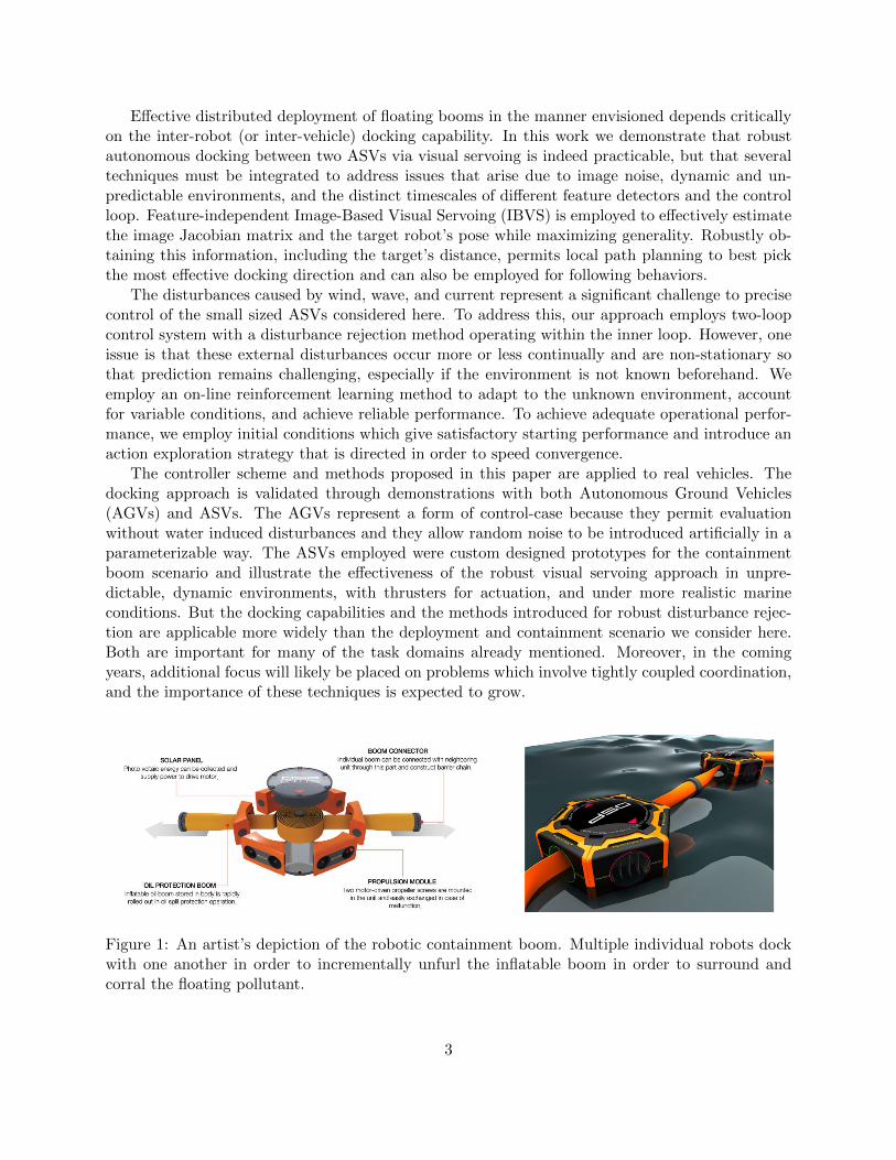
This paper describes a prototypical multi-robot system for deploying floating containmentbooms. We propose a distributed approach in which several ASVs incrementally form a chainaround the floating contaminant. Figure 1 is an artist’s rendering of the concept. Individualrobotic units are deployed in parallel and, potentially, in a number of different ways (e.g., eitherlaunched from a single vessel, thrown from several separate manned craft, released from the shore,or a combination of these options). Irrespective of their initial arrangement, the self-propelledunits maneuver in order to position themselves for maximum advantage. Next, a process of chainconstruction occurs. Pairs of robots dock with one another in an operation that causes their boomconnectors to interlock. As the units move apart, the connecting booms unreel to their full length.This chain formation process starts from one end and proceeds incrementally until the whole chainhas been formed. The units, physically coupled in this way, maintain the chain and their propulsionstill permits collective control of the barrier.

2

Effective distributed deployment of floating booms in the manner envisioned depends criticallyon the inter-robot (or inter-vehicle) docking capability. In this work we demonstrate that robustautonomous docking between two ASVs via visual servoing is indeed practicable, but that severaltechniques must be integrated to address issues that arise due to image noise, dynamic and un-predictable environments, and the distinct timescales of different feature detectors and the controlloop. Feature-independent Image-Based Visual Servoing (IBVS) is employed to effectively estimatethe image Jacobian matrix and the target robot’s pose while maximizing generality. Robustly ob-taining this information, including the target’s distance, permits local path planning to best pickthe most effective docking direction and can also be employed for following behaviors.

The disturbances caused by wind, wave, and current represent a significant challenge to precisecontrol of the small sized ASVs considered here. To address this, our approach employs two-loopcontrol system with a disturbance rejection method operating within the inner loop. However, oneissue is that these external disturbances occur more or less continually and are non-stationary sothat prediction remains challenging, especially if the environment is not known beforehand. Weemploy an on-line reinforcement learning method to adapt to the unknown environment, accountfor variable conditions, and achieve reliable performance. To achieve adequate operational perfor-mance, we employ initial conditions which give satisfactory starting performance and introduce anaction exploration strategy that is directed in order to speed convergence.

The controller scheme and methods proposed in this paper are applied to real vehicles. Thedocking approach is validated through demonstrations with both Autonomous Ground Vehicles(AGVs) and ASVs. The AGVs represent a form of control-case because they permit evaluationwithout water induced disturbances and they allow random noise to be introduced artificially in aparameterizable way. The ASVs employed were custom designed prototypes for the containmentboom scenario and illustrate the effectiveness of the robust visual servoing approach in unpre-dictable, dynamic environments, with thrusters for actuation, and under more realistic marineconditions. But the docking capabilities and the methods introduced for robust disturbance rejec-tion are applicable more widely than the deployment and containment scenario we consider here.Both are important for many of the task domains already mentioned. Moreover, in the comingyears, additional focus will likely be placed on problems which involve tightly coupled coordination,and the importance of these techniques is expected to grow.

Figure 1: An artist’s depiction of the robotic containment boom. Multiple individual robots dockwith one another in order to incrementally unfurl the inflatable boom in order to surround andcorral the floating pollutant.

3

The remainder of this paper is organized as follows: Section 2 describes the relationship betweenthis and existing work. Section 3 briefly describes the physical and logical system architecture.Section 4 explains the integrated visual servoing and control scheme. The experiments in Section 5demonstrate the performance with both ASV and AGV robots; the data are discussed in thatsection too. The final section, Section 6, concludes the paper.

2 Related Work

We are not aware of any prior work that considers autonomous deployment of booms, surfacepollutant containment, or incremental formation of tethered chains by surface vehicles. The conceptof distributed oil clean-up was recently proposed by Kakalis and Ventikos [2008]; while that workincludes conceptual pictures of “vacuum cleaner” like robots for collecting oil; we are not ableto assess the viability of that concept for use with physical robots. The approach we propose isbased on current oil spill management practice and is applicable to general containment of a varietyof matter (e.g., floating ice). Additionally, it can be sensible to deploy these boom devices as aprecautionary measure: their long-term effectiveness does not depend on significant movement orensuring wide-spread coverage.

The broad advantages that multi-robot systems have over single robot systems are directly ap-plicable to ASVs: viz. robustness through redundancy, performance speed-up through parallelism,expanded collective capability through synergy, and ability to exploit the distributed nature in-herent to certain tasks [Parker, 2008]. But within the literature there remain comparatively fewdemonstrations of multiple autonomous surface platforms. By way of examples: Benjamin etal. [2006] implement and demonstrate US Coast Guard mandated rules for prevention of collisions,and evaluate their implementation on multiple ASVs. Curcio et al. [2005] developed the SCOUT(Surface Craft for Undersea and Oceanographic Testing) surface vehicle as a platform for multiplevehicle operations algorithm testing, including underwater craft. The majority of multi-ASV workdoes not consider tightly-coupled coordination tasks where physical contact is necessary.

Within the broader autonomous marine vehicle literature, docking is an important instance inwhich a direct physical coupling is sought. Often underwater craft that explore the ocean floor,for example, may only recharge their batteries and transmit data when docked—either to a seabedstation or an ASV. Murarka et al. [2009] and Park et al. [2009] both use structured light for dockingtheir Autonomous Underwater Vehicle (AUV). The light serves as a reference signal which helpsthe robots approach the docking target. This is a particularly shrewd choice of positioning signalbecause the water’s filtering and attenuation can reduce the effect of external elements such assunlight, illumination changes, and artificial light, which cause interference on the surface. Thepresent study employs vision-based methods for inter-robot docking; we focus on the relationshipto work employing such methods in the remainder of this section. It is worth noting, however, thatalternative sensors have been used for docking (e.g., Kim et al. [2009] use RF signals), but thisleads to a new set of challenges.

Docking via Visual Servoing

Vision-based systems have been previously been shown to be effective for docking an ASV withan AUV. Martins et al. [2007] and Dunbabin et al. [2008] are good examples of coordinated ASVto AUV docking. That work makes creative use of their particular hardware: a vision camera is

4

fixed to the roof of the ASV and special angles are used to maximize detection of the AUV’s salientcolor. In this work, we are unable to use the same configuration since the robots we employ arehomogeneous and the focus on inter-robot docking means that no particular robot is privilegedso as to form a special drifting target. The solution employed in the present study—detailed inthe following section—is to employ visual feature descriptors and feature matching. This provedto be effective at accurately determining the distance to a target object and it was less sensitiveto lighting changes and more robust to scale variance than color segmentation (see Section 5.1).The majority of examples in the literature that successfully employ black and white, and colorsegmentation methods are for submerged operations (e.g., underwater line-following [Bibuli et al.,2008; El-Fakdi and Carreras, 2008]). The fundamental trade-off is that feature-based techniquesare more computationally expensive; the control architecture we employ, however, overcomes thelatency which arises from the slower detection and tracking.

Researchers attempting to perform visual servoing must address the issues of measurement noise,the limited computational time, and imperfect system models. There are two broad types of ap-proach: Position-Based Visual Servoing (PBVS) and Image-Based Visual Servoing (IBVS) [Hutchin-son et al., 1996]. Generally speaking, PBVS is robust to image noise but object information is re-quired to predict the object pose; PBVS is particularly sensitive to camera calibration and usuallyrequires a sophisticated model of the target (e.g., a CAD model). In contrast, IBVS does awaywith those requirements. It is largely robust to camera calibration error, but the image Jacobianmatrix depends on both the camera and the 3-D coordinates of the feature points. (Section 4.4describes how these elements are computed in the IBVS method we use.) SIFT [Lowe, 2004] basedtrackers, like those employed in this work, have been used in dynamic multi-vehicle settings be-fore. Most closely related is the system that Giesbrecht et al. [2009] developed as a step towardautonomous ground vehicle conveys. They address the problem of autonomously following a leaderand demonstrate this with on- and off-road vehicles. They face the same problem of comparativelyslow feature tracking, recognizing that obtaining data at the proper frequency is critical for thesystem to work well. Their approach is to reduced the search space so as to save computationaltime. Instead, this work uses an enhanced SIFT detector within a two-loop control architecture forcontrolling the ASV (see Section 4.2).

Modeling Environmental Disturbances via Reinforcement Learning

Prior work on ASV-to-AUV docking presumes that the latter is drifting on the water, and thewater itself is assumed to be calm. In this work we are concerned with docking quickly withboth a poor a priori understanding of the environment and potentially changing ocean conditions.Thus, the proposed method applies an on-line learning approach to the ASV control problem. Weillustrate how tabular SARSA(λ) [Sutton and Barto, 1998] will achieved convergence. Importantrelated work is the visual servoing control method of Martinez-Marin and Duckett [2005], who applyIBVS and reinforcement learning in a grasp positioning scenario. We believe Gaskett et al. [1999],who employed Q-learning and a neural network, were the first to apply reinforcement learning toAUVs. In contrast to our model-free approach, Pereira et al. [2008] employ a simplified model ofASV dynamics in order to perform station keeping with an under-actuated system. Fahimi [2007]develops sliding-mode control for ASVs, but relies of assuming disturbances are always of somemaximum amplitude. A learned model, like that which we employ, will likely result in betterperformance in a particular environment because the model can adapt to the structure of thatenvironment by learning that structure in situ.

5

Figure 2: Physical and logical architecture of the overall containment boom deployment system.

3 Physical System Architecture

We describe the overall architecture of an approach we envision for autonomous containment boomdeployment. Physically, the system consists of a single monitoring station and multiple autonomousrobots as shown in Figure 2. The monitoring station receives information about the spill config-uration and transmits target positions to each of the robots via wireless communication. Theseway-points (in GPS coordinates) are used both during initial positioning before the chain has beenformed and after booms are deployed to actively corral the floating oil. Each robot is autonomous,locally filtering and fusing several sensors, estimating properties of the environment, and capableof docking with other units without any external low-level guidance.

Each robot periodically transmits its estimated location back to the monitoring station so as toupdate the visual display; this information is used by the operator to assess the navigation progressof each unit with respect to the oil. The window in Figure 2 shows a simple interface in whicha region is selected with the mouse via rubber-band-like process. Target way-point locations arecomputed by dividing the circumference appropriately. Once satisfied with the relative position ofrobots and contaminant, the operator sends a chain formation command, which kicks off a processof docking around the perimeter. The robots dock in the following manner. An initially selectedrobot docks with the robot nearest to it along the boundary. Those two robots separate and theboom unfurls between them. Those two robots then hold their positions in order to become dockingtargets for their neighboring robots. The process continues until all the booms have been unfurled.Each robot adapts to its local environment, predicts its own position, and maintains its own status.When the docking operation is triggered, the robot which still has no boom unrolled is given onlythe GPS coordinate of the other unit. Although the error in this coordinate is too large for dockingdirectly, it is precise enough to allow the robot to get the target within its visual field of view.Visual servoing is used to obtain the precision necessary to complete the docking procedure.

The monitoring station manages information about the containment area but relies on eachrobot to autonomously perform its docking. Apart from the high-level directives, the stationserves to keep track of the overall scenario and watch the development of the chain. This paperdemonstrates that this architecture is logical and feasible because the robots can receive high-leveldocking commands and autonomously perform the necessary low-level controls to carry them out.

6

Figure 3: Autonomous Surface Vehicle designed as a prototype system in order to assess thefeasibility of a robotic containment boom deployment. These units are the primary platform usedfor implementation, development and validation of the robust visual servoing and docking behaviors.

Consequently, the bulk of the paper concentrates on visual servoing in order to dock in dynamic,unpredictable environments.

3.1 Prototype Hardware Units

The prototype ASV we developed is shown in Figure 3. This vehicle is the principal experimentalplatform for the development and testing of robust docking. Each ASV has three parts: an upperbody, a middle body and lower body. Upper body includes the main CPU, sensor board, andpower manager. The middle body add buoyancy to ensure that the ASV stays afloat. The lowerbody houses the motor driver and battery; these heavy components ensure the proper center ofgravity. The single camera is positioned at the midpoint of the front side pointing forward. Thetwo thrusters are positioned so that when both have equal power the unit moves forward, i.e., in

Figure 4: Test navigation of a single unit on a calm day.

7

the same direction as the camera is pointing. Figure 4 shows the wake pattern of the device whilenavigating. The hardware provides a selection of sensors which are ultimately fused in software toorder deal with unpredictable dynamic environments; environmental state estimation is managed bytwo micro-controllers (Atmega128, TMS320F28335) which mange sensors at a variety of samplingrates (a) GPS (66ch, DGPS): 500ms, (b) Compass (HMC6352, 2-axis): 250ms, (c) IMU (ADIS16350with 3-axis accelerometer and gyro): 100µs. The main CPU, an Intel core 2 duo at 1.8GHz, performsthe vision processing and manages high-level control.

Figure 5: Each robot’s controller software consists of two modules: the Control Logic Module andthe Vision Processing Module. The two switches labelled A and B permit separate activation anddeactivation of the modules. A sequence of switch settings allows robust docking with neighborrobots to be performed.

Figure 6: The Target Detection procedure within the Vision Processing Module follows a threestage pipeline, with each stage performed sequentially: (1) keypoints are extracted from the currentimage, (2) feature descriptors are computed for each keypoint, and (3) a match to the previous imageis found and outliers discarded.

8

4 Integrated Visual Servoing Control Scheme

Each robot runs controller software that is cleanly decomposed into two modules. Figure 5 showsthe two modules: the Control Logic Module, the Vision Processing Module, and their interactions.Three separate modes of behavior are realized by activating the modules in different ways via thetwo switches labelled A and B. The Control Logic Module is the primary procedure for controllingnavigation of the ASV. Its internal logic and novel integration of several components are describedin Section 4.2. The Visual Processing Module is responsible detecting and tracking other robots.

Initially the robot attempts to navigate toward the target as assigned to it by the monitoringstation. The Control Logic Module will operate in a global positioning mode, wherein input fromthe Vision Processing Module is unnecessary. Uncertainty due to imprecision in the GPS signalmeans that the robot cannot dock with that position information alone. Consequently, VisionProcessing Module must detect a target robot. After successful detection, the Vision ProcessingModule provides tracking information to the Control Logic Module, which it uses to navigate towardthe target. While doing this, other aspects of the control system (like disturbance compensation,for example) are operating concurrently.

4.1 The Vision Processing Module

The Vision Processing Module operates first in Target Detection mode and then transitions to theTarget Tracking mode during the final phase of tightly coupled docking. Figure 6 shows the se-quential pipeline involving three main procedures for the detection mode of operation: (1) keypointextraction; (2) feature descriptor computation, and (3) matching to a reference along with outlierremoval. Particular experiences and implementation choices are described for each of these next,along with the details of operation within the tracking mode.

Keypoint Extraction Given an input frame from the camera, the first operation is to extractfeatures for subsequent processing. Three requirements must be met: we must be able toidentify and extract features reliably, they must persist (or reoccur) across frames at least forsome short time-window, and processing must be efficient. These requirements become mostimportant when addressing the challenge of target detection under conditions arising fromsimultaneous target and camera motion in a dynamic environment. We implemented Rosenand Drummond’s FAST keypoint extractor. As shown in Rosten and Drummond [2006], themethod has the benefit of computational efficiency which enables high-speed corner detection.

Feature Descriptors The keypoints identified in the preceding step are particular points in theinput image. The property of invariance to changes in scale and orientation ensures thatsimilar views of the same scene will produce overlapping keypoint sets. A richer descriptorfor each keypoint must be computed in order to reliably associate the points between frames.Ideal feature descriptors will be maximally distinctive while being invariant to artefacts aris-ing from the camera and environment. In this work, robustness to changes in illuminationturned out to be especially important. We employed SIFT [Lowe, 2004] descriptors, which areinvariant to image translation, scaling and rotation, and partially invariant to illuminationchanges and robust to local geometric distortion.

Matching As a final process of target detection, a reference image’s feature points and an inputframe’s feature points must be correctly matched. This process is necessary in order to

9

estimate the target object’s position and to remove outliers. Iterative matching for eachpoint, while capable of finding the best possible matching, is computationally costly andwould adversely affect the performance of the entire vision pipeline. Computational savingsresult from selecting PROSAC [Ondrej Chum and Jiri Matas, 2005] over RANSAC (RandomSample Consensus) [Fischler and Bolles, 1981]. Significant speed results from exploiting alinear ordering structure for the matching, which requires assumptions that are reasonablymet in operation (a similarity measure must predict correctness of a match better than randomguessing).

Tracking The detection mode seeks to recognize, identify, and locate the target object by process-ing a single image in isolation. Since the detection mode considers all the pixels within theimage, significant processing cost (in terms of time) is incurred, which motivated our devel-opment of the tracking module. The tracking module is designed to exploit spatio-temporallocality: once the target object has been detected, the next target position is likely to be nearthe previous one. The system architecture includes a mechanism to permit smooth transitionfrom detection mode to tracking mode and back again. Figure 5 shows this with the symbolmarked Switch A; it obeys the following logic: when the target detection module succeeds indetermining the target object’s position, that information is provided to the tracking code forprocessing subsequent frames; if the target object is missed in target tracking mode, the visionprocessing is switched back to detection behavior as and when needed. Thus, the trackingmode serves to complement the detection mode. Our implementation uses a simple Mean-Shift Matching [Comaniciu et al., 2002] to track a target object. This method uses the colorhistogram of the object in the previous image to find the target object near the object’s pastposition. The simplicity of the method made it an attractive candidate for implementationand it proved to be adequate for the salient orange robots.

4.2 The Control Logic Module

The Control Logic Module is responsible for controlling the navigation of the ASV and is composedof the most critical elements of the control system. Figure 7 gives a graphical representation thecontroller. The figure shows three control loops: (1) the inner control loop, which is always active;(2) outer control loop-A, which is responsible for visual servo control and only active during thatmode of operation ; and (3) outer control loop-B, which is the global positioning control logic andis active while the robot is approaching the target from afar. Since exactly two control loops areactive at any one time, we term this a two-loop switching architecture. The two control loops areswitched when the robot is ready for docking.

The use of two loops permits the control system to minimize latency even though the timerequired for processing vision data can be significant. The visual servo control (marked as “outercontrol loop-A” reproduced in Figure 7) detects and recognizes a target objects and estimates anobject’s pose. It does this at comparatively slow speeds considering the dynamics of the robot.However, simultaneously, the tracker in the inner control loop (“inner control loop” in Figure 7)tracks the object at a high speed. A primary objective of the architecture was to abstract away theparticular choice of feature tracker and detector. This abstraction is only possible when the otherresponses of the system are not affected. Although not a perfectly clean abstraction, our approachenlarges the visual servo system’s feature independence and does permit multiple features to beused. The result is that the logic ultimately improves docking the target object because we were

10

Figure 7: A block diagrammatic overview of the Control Logic Module: three control loops arevisible. The inner loop is common and always active, but only one of the outer control loops is everactive at one time.

able to explore various feature choices.On the other hand, in global positioning mode (marked as “outer control loop-B” in Figure 7) is

applicable when approaching a target object from afar. Global position from the DGPS (DifferentialGlobal Positioning System) sensor has an uncertainty of almost ±3m in real environments. So thecontrol logic also helps in approaching the target object. The target’s position is communicatedfrom main station, and the outer control loop computes heading updates only at the GPS samplingfrequency (every 0.5s). The inner control loop (“inner control loop” in Figure 7) is able to applydisturbance rejection (along with reinforcement learning, as is explained at the next subsection)concurrently.

Thus, the inner control loop ensures accurate docking and way-point following. It managesto do this because of the box labelled “Local Position” in the block diagram, which includes adisturbance rejection mechanism (Compensator) to help overcome environmental dynamics. The“Compensator” employs high-frequency IMU data in order to address the effects of environmentaldisturbances, rather than relying on visual or GPS-based sensory feedback.

4.3 Disturbance Rejection

Figure 7 shows the inner control loop with a block labelled “compensator” which reduces theeffect of disturbances in an effort to maximize the range of circumstances in which the system

11

may robustly navigate. Navigation behavior is implemented through a combination of a traditionalcontrol scheme and Reinforcement Learning. The traditional control scheme involves a filteringapproach that is similar to that employed by Caccia et al. [2008]: we apply a state-space model ofthe Inertial Measurement Unit (IMU) and Kalman filter to estimate accelerations and deal withmeasurements’ noise characteristics since the measured accelerations contain errors such as drift.Even in relatively benign environments, prior work using Image-Based Visual Servoing for tracking(e.g., Aull [2009]) has emphasized the need for filtering of target locations. Ultimately, the approachwe employ relies on the use of linear accelerations to measure environmental disturbances.

In order to measure disturbance exerted by dynamic environments, a low-cost, strap-down,solid-state IMU is used in our system. The IMU consists of three accelerometers and three angularrate gyros. The three accelerometers measure linear accelerations in three perpendicular directionsand three gyros measure angular velocities in the same directions. The gyros are used to estimatethe robot’s attitude and the estimated attitude is applied to compensate for the local gravity inthe measured accelerations.

The local gravity can be calculated if its initial value or the robot’s initial orientation is known.In case of the former, using the given initial gravity and rotational angles obtained by the integrationof the angular velocities, the tri-axial components of the local gravity can be computed. In thelatter case, the attitude of the robot system is dependent on the initial orientation because theangular rates from the gyros are integrated to get the orientation angles of the robot system.Thus, the initial orientation of the robot system is needed to estimate accelerations from dynamicenvironments more correctly. Therefore, we adopt the former approach in our system.

4.3.1 Inertial Measurement Unit Model

To define the IMU model for detecting and hence rejecting disturbances, we choose a state vector

x =[xx

T xyT xz

T]T

(1)

where xm = [vm am bam ωm bωm]T is a state vector and vm, am, bam, ωm and bωm arevelocity, acceleration, acceleration bias, angular velocity, and angular velocity bias of the robotwith respect to the m-axis, where m ∈ {x, y, z}.

Using the state vector defined above, state-space equations for the IMU are given by [Farreland Barth, 1998; Grewal et al., 1991]:

x(k + 1) = x(k) + Gu(k) + n(k), (2)

y(k) = Hx(k) + v(k). (3)

(The details of these equations appear in Appendix A.)In the above equations, we assume all the process noises are uncorrelated with one another, and

accelerations and angular velocities along x-, y-, and z-axes can be observed independently. In orderto overcome the biased and non-stationary behavior of the IMU and to estimate the magnitudeof errors, the bias terms, bam and bωm related to the accelerometers and gyros, are modeled asundergoing a random walk and considered as states.

As the state-space equations show, the resulting process and measurement equations are alllinear, and the error states (bam and bωm) and their relevant true states (am and ωm) are coupledonly through the measurement equations but not process equations.

12

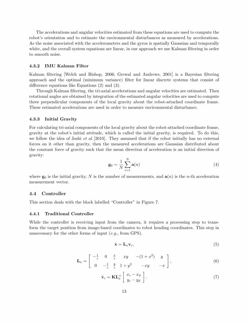
The accelerations and angular velocities estimated from these equations are used to compute therobot’s orientation and to estimate the environmental disturbances as measured by accelerations.As the noise associated with the accelerometers and the gyros is spatially Gaussian and temporallywhite, and the overall system equations are linear, in our approach we use Kalman filtering in orderto smooth noise.

4.3.2 IMU Kalman Filter

Kalman filtering [Welch and Bishop, 2006; Grewal and Andrews, 2001] is a Bayesian filteringapproach and the optimal (minimum variance) filter for linear discrete systems that consist ofdifference equations like Equations (2) and (3).

Through Kalman filtering, the tri-axial accelerations and angular velocities are estimated. Thenrotational angles are obtained by integration of the estimated angular velocities are used to computethree perpendicular components of the local gravity about the robot-attached coordinate frame.These estimated accelerations are used in order to measure environmental disturbance.

4.3.3 Initial Gravity

For calculating tri-axial components of the local gravity about the robot-attached coordinate frame,gravity at the robot’s initial attitude, which is called the initial gravity, is required. To do this,we follow the idea of Joshi et al. [2010]. They assumed that if the robot initially has no externalforces on it other than gravity, then the measured accelerations are Gaussian distributed aboutthe constant force of gravity such that the mean direction of acceleration is an initial direction ofgravity:

g0 =1

N

N∑i=1

a(n) (4)

where g0 is the initial gravity, N is the number of measurements, and a(n) is the n-th accelerationmeasurement vector.

4.4 Controller

This section deals with the block labelled “Controller” in Figure 7.

4.4.1 Traditional Controller

While the controller is receiving input from the camera, it requires a processing step to trans-form the target position from image-based coordinates to robot heading coordinates. This step inunnecessary for the other forms of input (e.g., from GPS).

x = Lxvc, (5)

Lx =

[−1

z 0 xz xy −(1 + x2) y

0 −1z

yz 1 + y2 −xy −x

], (6)

vc = KL+x

[xc − xdyc − yd

]. (7)

13

Equation (5) relates the image plane feature velocity x to the fixed camera velocity vc. Therelationship between the two relies on Lx, the image Jacobian which is shown in Equation (6), wherez is the target object’s depth. Since feature distance is computed from vision information, the Lx

can be calculated directly from known variables. The image plane feature position is (xc, yc). Thedesired feature position is (xd, yd). The traditional PID controller is constructed in Equation (7)where L+

x is Pseudo-inverse of Lx.

4.4.2 Reinforcement Learning

A variety of different learning methods exist within the reinforcement learning literature. Thepresent task requirements dictate that we address a control problem without a complete priormodel of the environment dynamics. Two additional (and inter-related) constraints direct thechoice of method: firstly, the requirement for reasonable actuator controls from the very beginning,and, secondly, a preference for rapid convergence. SARSA, named because it learns from thevariables abbreviated as (st, at, rt+1, st+1, at+1), is an algorithm which estimates a state-action–value function (or Q-function) for a given policy. SARSA is a popular application of the temporaldifference approach to address control problems. The algorithm forms an intermediate methodbetween TD(0) and the Monte-Carlo method being both model-free and capable of boot-strapping.Consideration of at+1 is what distinguishes SARSA from standard Q-Learning: the Q-values in theformer represent the values for the policy the learning agent follows including the consequences ofexploration, while the latter considers only the values from following a exploitation policy. Putanother way, in SARSA a policy describes the action selected in a particular state (st) with theaction performed in the next state (st+1) drawn from the same policy; thus, it is called an on-policymethod.

One advantage of SARSA is the ease with which it can be extended to allow eligibility tracesin the form of a method called SARSA(λ). An eligibility trace is additional information associatedwith each Q-value which records the visits to the associated state. The eligibility trace does thisin a time-decaying manner (we employ the notation e(s, a) below for this information). The tracevalue is interpreted as the degree to which a particular Q-value is suited for learning updates,which means the temporal difference information can update many values rather than a single one.Thus, SARSA(λ) has the advantage that learning time can be greatly accelerated over the standardSARSA method.

In the implementation and evaluation described below, we have introduced a new action selec-tion policy which augments a basic policy by imposing additional structure on the non-exploitativeactions. We term this “exploration guidance” because it uses the current Q-value maximum toinfluence exploration choices. In particular, we found that the vast majority of exploratory actionscan be drawn from boundary conditions that are essentially useless because they ignore the struc-ture already identified via the maximum Q-value. When appropriate initial conditions are used(as described below) exploration guidance tempers the actions that are selected so that reasonablecontrol is achieved throughout the learning process. Essentially, the method enforces a bound onthe difference between the exploration and the exploitation actions, via a parameter σe. So doingadds the additional requirement that there be a measure of difference between actions, which isquite natural in our control context. The algorithm, from Sutton and Barto [1998], is shown inAlgorithm 1 along with the modifications that add exploration guidance. The pseudo-code showshow an action selection based on the ε-greedy policy can use the σe guidance; treatment for ε-soft,or softmax variations are analogous.

14

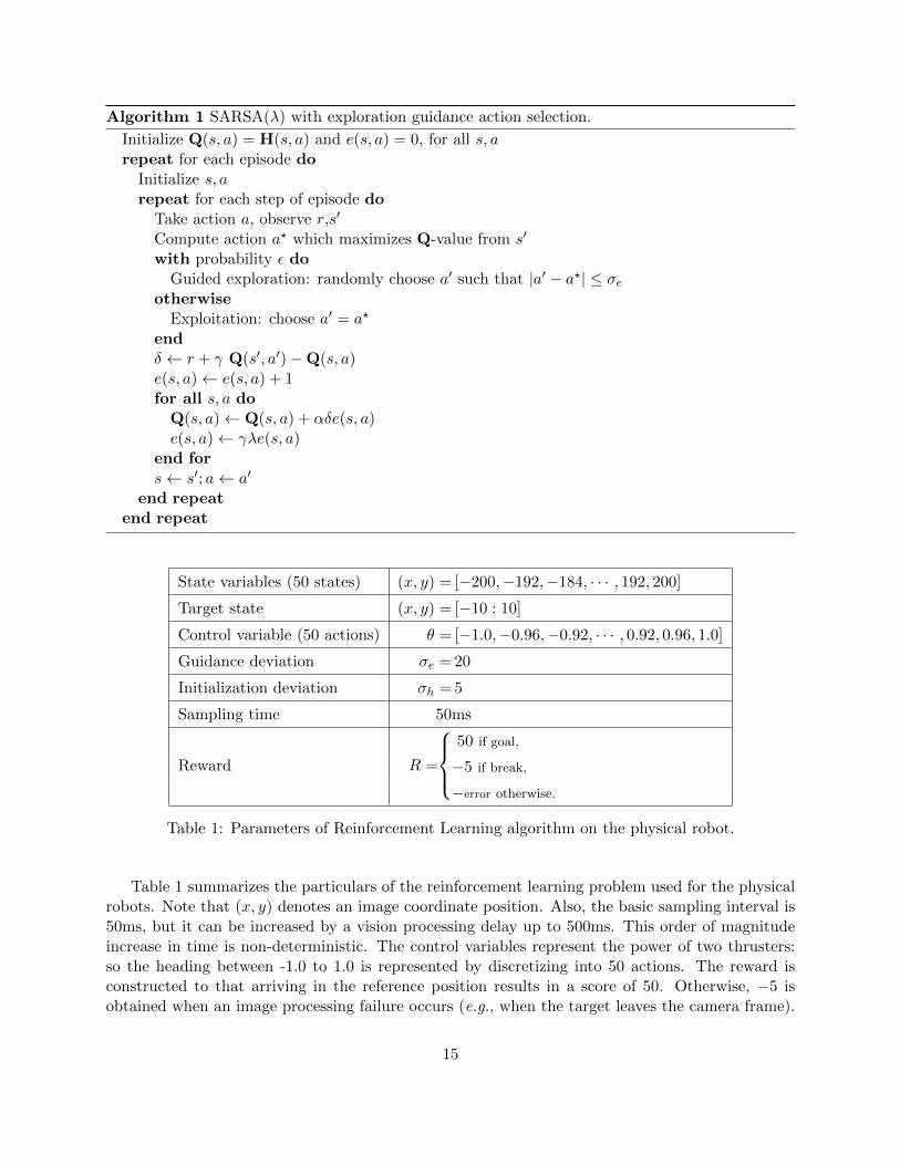
Algorithm 1 SARSA(λ) with exploration guidance action selection.

Initialize Q(s, a) = H(s, a) and e(s, a) = 0, for all s, arepeat for each episode do

Initialize s, arepeat for each step of episode do

Take action a, observe r,s′

Compute action a? which maximizes Q-value from s′

with probability ε doGuided exploration: randomly choose a′ such that |a′ − a?| ≤ σe

otherwiseExploitation: choose a′ = a?

endδ ← r + γ Q(s′, a′)−Q(s, a)e(s, a)← e(s, a) + 1for all s, a do

Q(s, a)← Q(s, a) + αδe(s, a)e(s, a)← γλe(s, a)

end fors← s′; a← a′

end repeatend repeat

State variables (50 states) (x, y) = [−200,−192,−184, · · · , 192, 200]

Target state (x, y) = [−10 : 10]

Control variable (50 actions) θ = [−1.0,−0.96,−0.92, · · · , 0.92, 0.96, 1.0]

Guidance deviation σe = 20

Initialization deviation σh = 5

Sampling time 50ms

Reward R =

50 if goal,

−5 if break,

−error otherwise.

Table 1: Parameters of Reinforcement Learning algorithm on the physical robot.

Table 1 summarizes the particulars of the reinforcement learning problem used for the physicalrobots. Note that (x, y) denotes an image coordinate position. Also, the basic sampling interval is50ms, but it can be increased by a vision processing delay up to 500ms. This order of magnitudeincrease in time is non-deterministic. The control variables represent the power of two thrusters:so the heading between -1.0 to 1.0 is represented by discretizing into 50 actions. The reward isconstructed to that arriving in the reference position results in a score of 50. Otherwise, −5 isobtained when an image processing failure occurs (e.g., when the target leaves the camera frame).

15

We have assumed that the camera is located and aligned so the central region of the imagecoincides with a straight heading. Using this information, an initial state-action table with reason-able starting values is constructed. This is done via a 50 × 50 matrix H composed to have valuesfor treatment of each control variable (−1.0 < A < 1.0, a total of 50 actions) in each possible state(−200 < S < 200, a total of 50 states). We impose the following natural relationship betweenactions and states: alignment means that the indices can be directly associated. For each state (acolumn in H) we assign values in the form of a Gaussian probability distribution across the actions(the row entries). The distribution has a constant standard deviation given by σh, but is shiftedso that the peak in column i falls in the ith position. Thus, the maximum values fall along thediagonal of H. As the number of episodes is increased and additional empirical data is obtained,the Q matrix adapts to better reflect the dynamic, unpredictable environment. The purpose of His to help achieve operational robustness in the early stages of learning.

To sum up, we have employed two approaches to apply reinforcement learning techniques toour problem: one is using guidance exploration SARSA(λ) to help speed convergence, the other isdesigning an initial H matrix for stability.

4.5 Disturbance Compensation

Algorithm 2 describes the simple logic that implements the disturbance compensation methodin software: essentially it consists of two concurrently executing control loops, each operatingat a time-scale dictated by their inputs, which are coupled through heading variables. Dm =[yx

T yyT yz

T]T

is the output of the disturbance model (in m/s2) as is described in Section 4.3and detailed in Appendix A. Since the IMU coordinate system is aligned with the image framecoordinates in our system, the model of environmental disturbances can be simplified by consideringthe accelerations along the first two axes (viz.

[yx

T,yyT]). In the algorithm, Rpos denotes the

horizontal reference position in camera coordinates (i.e., the center of image, in our configuration).Tpos represents the current estimate of the target object’s position and is produced by the visionprocessing pipeline as outlined in Section 4.1. From the reference position and the target’s positionwe directly compute a heading which we denote with θt. Also θd represents the robot’s desiredheading which is computed to offset estimated disturbances. Finally, xd is the robot’s desiredspeed which is similarly adjusted.

The control loops are shown as each of the two main functions: The Outer Controllerwhich updates θt by using the measured target object position. The other is Inner Controllerwhich counteracts the disturbance by using Dm(yx

T,yyT). The disturbance elements yx

T and yyT

are used because they have the primary influence on the heading and speed of the robot. The gaingx is used in computing θd as described in the algorithm, and it serves to normalize the output tobetween −1 and +1 radians. The robot’s speed, xd is adjusted by gy similarly.

5 Experiments

The environment used for the marine experiments that follow was a flowing river. The experimentalscenario is shown in Figure 8. The global positioning mode is employed to have the ASV approachthe target object and get it within range before detection of the target object and visual servoingcommences. The docking target was passive: floating on the surface not executing any motorcommands, which we feel can help in evaluating the proposed method. Once visual servoing mode

16

Algorithm 2 Disturbance compensation via two loop controller

Inputs:

Dm = Disturbance measurement[yx

T yyT yz

T]T

(acceleration along each axis)Rpos = Reference position [x] in camera coordinatesTpos = Target object position [x, y] in camera coordinates

Parameters:gx,y = The gain parameter of computing θd and xs = The robot’s pre-adjusted speed

Computed Values:θt = The direction to the target object by image processingθd = The robot’s desired headingxd = The robot’s desired speed

Function Outer Controller(Tpos, Rpos) (update θt when the vision is processed)θt = Rpos − Tpos(x)

Function Inner Controller(θt, Dm) (update θd and xd when the IMU is processed)θd = θt − gxDm(X)xd = s− gyDm(Y )

Figure 8: The evaluation scenario: flowing water with wind typical of unpredictable dynamicenvironments which are challenging to model.

17

is enabled the target object was reliably. ASV operates autonomously employing the controllerdescribed. Measurements were made of whether the ASVs docked; final docking was deemedto have been achieved only when contact was made between robots. Since we were unable toinstantaneously measure the flowing river, ground truth (e.g., with different degrees of disturbanceand noise) for evaluation purposes remained problematic. Thus, we also used the same controllers onground vehicles: with the AGVs we assume that ground is static easily characterizable environmentcompare to a choppy, flowing water surface. With the ground vehicles, synthetic noise was addedfor comparison to the no noise case. Although only an approximation, we believe this to be a goodpreliminary evaluation of the impact of the disturbance compensation mechanism. The final wetest we carried out was with ASVs in a realistic marine environment, and the results show thatthe proposed disturbance rejection, reinforcement learning, and two-loop controller permit dockingin unpredictable and dynamic environments. Moreover, comparison to the traditional controllerresults show the effectiveness of the disturbance rejection method.

5.1 Depth Estimation in Visual Servoing

Most image features have different processing times. Particularly, SIFT [Lowe, 2004] performswell in detecting and recognizing a target object in real environment. However, because of slowcomputation time, it is insufficient for uses that require real-time performance. In order to use it inreal environments, Giesbrecht et al. [2009] uses a SIFT tracker to track a moving object. To do so,the authors measured the processing time for the SIFT computation and calibrated their controlloop so as to use this as the underlying control period. A reduction in search space was necessaryin order to maximize the control frequency.

In this paper, we employ a two-loop control logic in order to have a feature-independent ap-proach. Thus, our system can use feature descriptors such as SIFT in addition to a robust matchingmethod. Generally feature descriptors are comparatively slow, but they can successfully estimatea target object’s pose and depth both of which are useful for dynamic docking as well as following.In the following experiments, the scale of the target object (as a function of distance) is given by ascale table. Consequently, depth information is produced from scale. Figure 9 shows the detectedimage height versus ground truth distance for both SIFT and our matching method. While bothmethods have agreement over their common range, SIFT can detect up to 200cm while the trackercan track the target object up to 500cm. When both run concurrently, SIFT takes 1000ms perframe while the tracker uses only 100ms on our hardware.

It can support the estimated scales of the target robots. SIFT can detect up to 200cm within1000ms, while simultaneously, the tracker can track the target object up to 500cm within 100mswith our hardware. Thus, various features can be used for target object detection and tracking inthe proposed control architecture. To overcome the feature descriptors’ slow speed, several trackerscan be used within the inner controller, which helps to compensate for the detection speed andassists in tracking long distances.

The results of the tests on the detection and tracking of target objects in real environments areshown in Figure 10. The scale size represents robot’s depth which is from produced from the scaletable.

18

Figure 9: Scale Estimation: detected target image height versus ground truth distance for the slowSIFT features compared and our implementation of a tracking method.

Figure 10: Target detection (white boxes) and tracking (red boxes) for the AGV and ASVs.Left: Target Detection at 1m. Middle: Target Tracking at 2m. Right: Target Tracking at 4m.

19

Figure 11: A “docking” test with autonomous ground vehicles. This scenario permits controlledevaluation of the role of environmental disturbances since the AGVs do not contend with the effectsof choppy, flowing water or wind.

5.2 Results of Autonomous Ground Vehicle

To evaluate the proposed method, one target AGV was placed 4m ahead of another AGV. Thetarget AGV was detected AGV. Figure 11 shows the approach of the docking AGV along with itstracking on the right. The utility of disturbance rejection was evaluated by comparing a traditionalPID (with Reinforcement Learning) controller with disturbance rejection to one without. Onthe ground, there is not enough noise to reject disturbance. So, injected Gaussian noise is usedto capture elements of a dynamic, unpredictable environment. In Figure 11, number 1 showscompletion of approach control, and number 2 shows detecting and tracking the target robot withdisturbance rejection. Finally, number 3 is docked with the target robot.

As a result, in Figure 12, the left figure shows the results of Reinforcement Learning withoutdisturbance rejection which does not have irregular rewards at any time. The right figure showsthose of Reinforcement Learning with disturbance rejection: observe both the increased meanreward function, the reduction in variance, and the significantly improved lower envelope. Thissuggests the disturbance rejection improves the learning process itself.

Moreover, in Figure 13, we present two types of noise conditions for both the PID and RL con-trollers (left and right, respectively). The “No Added Noise” condition reflects the natural noisewithin the robot system, i.e., but without additional noise being injected. The “Random Noise”condition includes the addition of Gaussian random noise (horizontal position error is sampled froma Normal distribution with σ = 20 pixels.) The plots show the response of the system under eachof these conditions along with a third line illustrating the effectiveness of the controllers under the“Random Noise” condition but with the disturbance rejection functionality enabled. By comparingthe relative amplitude of the oscillations it is straightforward to observe that the ReinforcementLearning controller follows the target more smoothly than the traditional PID controller. Addi-tionally, disturbance rejection helps to follow a target object more smoothly in both cases. Finally,

20

Figure 12: An illustration of the effectiveness of disturbance rejection on the learned state-actionmap (Q-values): the Q-value function landscape is flattened and smoothed. The left figure showsthe Q-values of the executed policy versus time in four separate trials for Reinforcement Learningwithout disturbance rejection on docking ground vehicles. The right figure is identical except withdisturbance rejection enabled. Significant variations both along individual trials and between trialsis readily observed. Nevertheless the disturbance rejection reduces the amplitude of the Q-valuevariation. (Since SARSA is an on-policy method, the Q-values represent estimates of returnedreward including both exploration and exploitation aspects.)

Figure 13: Evidence of increased stability in visual servoing control on ground vehicles. The verticalaxis represents the distance of the centroid of the target from the central line in the image (in numberof pixels); the horizontal axis denotes time in seconds. Smoothness of the target following behavior isreflected in the relative amplitudes. (Left: PID controller, Right: Reinforcement Learning controllercontroller).

21

Figure 14: An example USV pair docking test. (Compare the water surface to the calm day shownin Figure 4.)

the combined use of disturbance rejection and Reinforcement Learning is beneficial. (Note that inFigure 13, the vertical axis represents object positions relative to the center of input images so zerois the target reference, permitting one to interpret the required robot heading.)

5.3 Results of Autonomous Surface Vehicles

The previous section demonstrated that the techniques integrated into the control system areeffective for AGV docking. Next, the system was tested with our prototype ASVs in a real riverenvironment. The scenario as described above. As shown in Figure 14, one ASV detect the otherASV and then docks with it. The fourth frame of Figure 14 is the view of ASV from the initialposition.

Tests in which the ASV tries to dock to a drifting target robot at a distance of 4m away wereexecuted for different initial poses but same distance and the results are reported in Figure 15.The dotted lines on both the graphs are results of PID & RL without disturbance rejection (twodifferent initial positions). The solid lines are results of PID & RL with disturbance rejection (threedifferent initial positions). In general, the particular initial positions give repeated fluctuation. ThePID controller has more frequent and large oscillation compared to the Reinforcement Learningmethod. Moreover, disturbance rejection reduces these fluctuation, and reduces the time needed toapproach the other robot. The shorter execution times suggest additional robustness to fluctuations,as reaching stability implied faster recover. As the number of time is increased which is shown DR1to DR3, the docking time is reduced from around 7 seconds to 5 seconds. Moreover, based on theoscillation, the Reinforcement Learning with disturbance rejection shows the stable visual controllercompared to the traditional approach.

Evidence of increased stability in visual servoing control on ground vehicles. The vertical axis

22

Figure 15: Visual servoing control of Autonomous Surface Vehicles at real environment. Thevertical axis represents the distance of the centroid of the target from the central line in theimage (in number of pixels); the horizontal axis denotes time in seconds. (Left: PID controller,Right: Reinforcement Learning controller controller).

represents the distance of the centroid of the target from the central line in the image (in number ofpixels); the horizontal axis denotes time in seconds. Smoothness of the target following behavior isreflected in the relative amplitudes. (Left: PID controller, Right: Reinforcement Learning controllercontroller).

6 Conclusions

Ultimately, if ASVs are to fulfill important search, rescue, navigation, and inspection duties, thesevehicles need to detect and recognize objects fast and reliably, and they need to be able to operatein unpredictable and dynamic environments. This paper has described an approach with severalintegrated elements toward that end:

• Visual servoing is generally considers a single control loop. However, this work used a two-loop system with a switching structure that increases feature generality. The visual servoingcontroller uses numerous features such as color, templates, and local descriptors, all of whichhave different extraction speeds, yet all of which can be used without serious restriction.Attempting to attain feature-independence in visual servo control is a useful principle inorder to achieve robustness and a two-loop switched controller is an effective way to do this.

• Disturbance rejection-like stabilization at the shortest time-scale is beneficial in dynamicenvironments, but can require selection of computationally efficient techniques (like the mean-shift, in our case). Fusing data at the longest time-scale is likely to be problematic.

• Adaptability via on-line learning improves performance in non-stationary environments, butcareful choice of learning algorithm and choice of sub-problem is important. In this work

23

Figure 16: Tests with multiple tethered units.

it remains unclear how disturbance rejection affects the learning process. Both disturbancerejection and adaptation improve performance; their interplay is not yet clear.

This work has proposed an important multi-ASV application: that of autonomous robotic boomdeployment in order to corral floating pollutants. Our experience was that wind, waves, and watercurrents would pose a particular challenge for tasks that require tightly coupled coordination. Aprototype robotic system was constructed, and the plausibility of autonomous multi-ASV dock-ing demonstrated, including evaluation with test-trials with controlled noise conditions on groundvehicles.

6.1 Outlook and Future Work

Further development is necessary before the robotic containment boom idea can be declared feasible.An important mechanical consideration is the mechanism by which booms should reliably fastenafter the docking procedure. Possibly insights from the reconfigurable robotics community couldcontribute to that solution. Figure 16 shows some preliminary experiments that were conductedwith the units that had been tethered together. Exactly how to maneuver large groups of suchrobots remains an open question.

Future work could consider ways in which the disturbance rejection scheme can be extendedthrough a robust three-axis modeling that can help the system adapt to additional types of chal-lenging environments. This would address limitations of the current approach and likely improveperformance across a range of dynamic environments. Second, while currently employing twocontrol loops helps ameliorate the effects of delay in sensor processing, faster feature extractionmethods will naturally improve the quality of the control output and can simplify the controlleritself. For example, the separation between target detection and tracking is critical to the successof the current system because detection on its own would be too slow. Third, important questionsremain as to the rate of convergence when adaptive on-line learning methods are used in multi-vehicle scenarios. For example, when two robots are approaching one another in order to dock,it would be beneficial to have an estimate of their comparative stability as this could affect theservoing strategy employed.

24

A IMU Model

State-space equations for the IMU are given by

x(k + 1) = Φx(k) + Gu(k) + n(k), (8)

y(k) = Hx(k) + v(k), (9)

where Φ = diag(Φx,Φy,Φz) is the state transition matrix and is a block diagonal matrix thatconsists of the state transition matrices

Φm =

1 Ts 0 0 00 1 0 0 00 0 1 0 00 0 0 1 00 0 0 0 1

, (10)

of each axis, where Ts is the sampling interval. The input matrix, G = diag(Gx,Gy,Gz) is

a block diagonal matrix with the input matrices, Gm = [Ts 0 0 0 0]T. The measurementmatrix, H = diag(Hx,Hy,Hz) is also a block diagonal matrix having three m-axis input matrices,

Hm =

[0 1 1 0 00 0 0 1 1

].

y =[yx

T yyT yz

T]T

is an output vector that is a compound of each axis’s output vector,

ym = [am ωm]T. Here am and ωm mean measurements of the accelerometer and gyro with respect to

the m-axis. A system’s input vector, u =[gx + aFx gy + aFy gz + aFz

]T. consists of components

along each axis of the local gravity, gm and of the acceleration, aFm exerted by the robot’ driving

force. n =[nx

T nyT nz

T]T

means a process noise vector of unmodeled effects with the pro-

cess noise vectors of m-axis, nm = [nvm nam nbam nωm nbωm ]T, each element of which meansGaussian white noise corresponding to each element of the state vector and nvm ∼ N(0, Qvm),nam ∼ N(0, Qam), nbam ∼ N(0, Qbam), nωm ∼ N(0, Qωm), and nbωm ∼ N(0, Qbωm). A measurement

noise vector, v =[vx

T vyT vz

T]T

is made up of each measurement noise vector, vm = [vam vωm]T

of axes where vam and vωm are Gaussian white noises corresponding to each element of the outputvector, ~ym, and therefore these noise terms are defined by vam ∼ N(0, Ram), and vωm ∼ N(0, Rωm).

References

[Aull, 2009] Mark Aull. Visual servoing for an autonomous rendezvous and capture system. Intel-ligent Service Robotics, 2(3):131–137, July 2009.

[BBC, 2007] BBC. South Korea fights huge oil spill, December, 10 2007.http://news.bbc.co.uk/2/hi/asia-pacific/7135896.stm.

[Benjamin et al., 2006] Michael Benjamin, Joseph Curcio, John J. Leonard, and Paul Newman.Navigation of Unmanned Marine Vehicles in Accordance with the Rules of the Road. In Pro-ceedings of the IEEE International Conference on Robotics and Automation (ICRA’06), pages3581–3587, Orlando, FL, May 2006.

25

[Bertram, 2008] Volker Bertram. Unmanned Surface Vehicles – A Survey. In Proceedings of Skib-steknisk Selskab Meeting, Copenhagen, Denmark, March 2008.

[Bibuli et al., 2008] Marco Bibuli, Gabriele Bruzzone, Massimo Caccia, Giovanni Indiveri, andAlessandro A. Zizzari. Line following guidance control: Application to the Charlie unmannedsurface vehicle. In Proceeding of the IEEE International Conference on Intelligent Robots andSystems (IROS’08), pages 3641–3646, Nice, France, September 2008.

[Caccia et al., 2008] Massimo Caccia, Marco Bibuli, Riccardo Bono, and Gabriele Bruzzone. Ba-sic navigation, guidance and control of an Unmanned Surface Vehicle. Autonomous Robots,25(4):349–365, November 2008.

[Clauss et al., 2009] Gunther F. Clauss, Andre Kauffeldt, and Nils Otten. AGaPaS — AutonomousGalileo-Supported Rescue Vessel for Persons Overboard. In Proceedings of International Con-ference on Ocean, Offshore and Arctic Engineering (OMAE’09), Honolulu, Hawaii, May 2009.

[Comaniciu et al., 2002] Dorin Comaniciu, Peter Meer, and Senior Member. Mean shift: A robustapproach toward feature space analysis. IEEE Transactions on Pattern Analysis and MachineIntelligence, 24(5):603–619, May 2002.

[Curcio et al., 2005] Joseph Curcio, John Leonard, and Nicholas Patrikalakis. SCOUT—a lowcost autonomous surface platform for research in cooperative autonomy. In Proceedings of theMTS/IEEE Oceans Conference, pages 725–729, Washington D.C.,, September 2005.

[Doerffer, 1992] Jerzy Doerffer. Oil Spill Response in Marine Environment. Pergamon Press, NewYork, NY, 1992.

[Dunbabin et al., 2008] Matthew Dunbabin, Brenton Lang, and Brett Wood. Vision-based DockingUsing an Autonomous Surface Vehicle. In Proceedings of the IEEE International Conference onRobotics and Automation (ICRA’08), pages 26–32, Pasadena, CA, USA, May 2008.

[El-Fakdi and Carreras, 2008] Andres El-Fakdi and Marc Carreras. Policy gradient based Rein-forcement Learning for real autonomous underwater cable tracking. In Proceeding of the In-ternational Conference on Intelligent Robots and Systems (IROS’08), pages 3635–3640, Nice,France, September 2008.

[Fahimi, 2007] Farbod Fahimi. Sliding-Mode Formation Control for Underactuated Surface Vessels.IEEE Transactions on Robotics, 23(3):617–622, June 2007.

[Fang and Wong, 2001] Jianzhi Fang and Kau-Fui V. Wong. Optimization of an Oil Boom Ar-rangement. In Proceedings of Biennial International Conference on Oil Spills, Tampa, FL, March2001.

[Fang and Wong, 2006] Jianzhi Fang and Kau-Fui V. Wong. An advanced VOF algorithm for oilboom design. International Journal of Modelling and Simulation, 26(1), January 2006.

[Farrel and Barth, 1998] Jay A. Farrel and Matthew Barth. The Global Positioning System andInertial Navigation. McGraw-Hill, New York, USA, 1998.

[Fingas and Charles, 2000] Mervin F. Fingas and Jennifer Charles. The basics of oil spill cleanup.CRC Press, 2 edition, 2000.

26

[Fischler and Bolles, 1981] Martin A. Fischler and Robert C. Bolles. Random Sample Consensus:A Paradigm for Model Fitting with Applications to Image Analysis and Automated Cartography.Comm. of the ACM, 24(6):381–395, June 1981.

[Gaskett et al., 1999] Chris Gaskett, David Wettergreen, and Alexander Zelinsky. ReinforcementLearning applied to the control of an Autonomous Underwater Vehicle. In Proceedings of theAustralian Conference on Robotics and Automation (AUCRA99), pages 125–131, Brisbane, Aus-tralia, March 1999.

[Giesbrecht et al., 2009] Jared L. Giesbrecht, Hien K. Goi, Timothy D. Barfoot, and Bruce A.Francis. A vision-based robotic follower vehicle. Proceedings of the International Society forOptics and Photonics (SPIE), 7332:733210–1–733210–12, April 2009.

[Grewal and Andrews, 2001] Mohinder S. Grewal and Angus P. Andrews. Kalman Filtering: The-ory and Practice Using MATLAB. Wiley-Interscience, New York, USA, 2001.

[Grewal et al., 1991] Mohinder S. Grewal, Vinson D. Henderson, and Randy S. Miyasako. Applica-tion of Kalman Filtering to the Calibration and Alignment of Inertial Navigation Systems. IEEETransactions on Automatic Control, 36(1):4–13, January 1991.

[Grier, 2010] Peter Grier. Containment boom effort comes up short in BP oil spill. The ChristianScience Monitor, June, 11 2010.

[Hutchinson et al., 1996] Seth Hutchinson, Gregory D. Hage, and Peter I. Corke. A Tutorial onVisual Servo Contol. IEEE Transactions on Robotics and Automation, 12(5):651–670, October1996.

[Joshi et al., 2010] Neel Joshi, Sing Bing Kang, C. Lawrence Zitnick, and Richard Szeliski. Imagedeblurring using inertial measurement sensors. ACM Transactions on Graphics, 29(4):1–9, July2010.

[Kakalis and Ventikos, 2008] Nikolaos M.P Kakalis and Yiannis Ventikos. Robotic Swarm Conceptfor Efficient Oil Spill Confrontation. Journal of Hazardous Materials, 154(1–3):880–887, June2008.

[Kim et al., 2009] Myungsik Kim, Nak Young Chong, and Wonpil Yu. Robust DOA estimationand target docking for mobile robots. Intelligent Service Robotics, 2(1):41–51, January 2009.

[Lowe, 2004] David G. Lowe. Distinctive Image Features from Scale-Invariant Keypoints. Interna-tional Journal of Computer Vision, 60(2):91–110, January 2004.

[Martinez-Marin and Duckett, 2005] Tomas Martinez-Marin and Tom Duckett. Fast ReinforcementLearning for Vision-guided Mobile Robots. In Proceedings of the IEEE International Conferenceon Robotics and Automation (ICRA’05), pages 4170–4175, Barcelona, Spain, April 2005.

[Martins et al., 2007] Alfredo Martins, J. M. Almeida, H. Ferreira, H. Silva, N. Dias, A. Dias,Carlos Almeida, and E. P. Silva. Autonomous Surface Vehicle Docking Manoeuvre with VisualInformation. In Proceedings of the IEEE International Conference on Robotics and Automation(ICRA’07), pages 4994–4999, Roma, Italy, April 2007.

27

[Murarka et al., 2009] Aniket Murarka, Gregory Kuhlmann, Shilpa Gulati, Mohan Sridharan,Christopher Flesher, and William C. Stone. Vision-based Frozen Surface Egress: A DockingAlgorithm for the ENDURANCE AUV. In Proceedings of the International Symposium on Un-manned Untethered Submersible Technology (UUST), New Hampshire, USA, August 2009.

[Murphy et al., 2011] Robin R. Murphy, Eric Steimle, Michael Hall, Michael Lindemuth, DavidTrejo, Stefan Hurlebaus, Zenon Medina-Cetina, and Daryl Slocum. Robot-Assisted Bridge In-spection. Journal of Intelligent & Robotic Systems, pages 1–19, 2011.

[NOAA, 2010] NOAA. Deepwater Horizon MC252 Gulf Incident Oil Budget, August, 2 2010.http://www.noaanews.noaa.gov/stories2010/PDFs/DeepwaterHorizonOilBudget20100801.pdf.

[Ondrej Chum and Jiri Matas, 2005] Ondrej Chum and Jiri Matas. Matching with PROSAC—Progressive Sample Consensus. In Proceedings of the IEEE Computer Society Conference onComputer Vision and Pattern Recognition, pages 220–226, San Diego,USA, July 2005.

[Park et al., 2009] Jin-Yeong Park, Bong huan Jun, Pan mook Lee, and Junho Oh. Experiments onvision guided docking of an autonomous underwater vehicle using one camera. Ocean Engineering,36(1):48–61, January 2009.

[Parker, 2008] Lynne E. Parker. Multiple Mobile Robot Systems. In Bruno Siciliano and OussamaKhatib, editors, Handbook of Robotics, chapter 40. Springer, 2008.

[Pereira et al., 2008] Avind Pereira, Jnaneshwar Das, and Gaurav S. Sukhatme. An ExperimentalStudy of Station Keeping on an Underactuated ASV. In Proceedings of the IEEE Interna-tional Conference on Intelligent Robots and Systems (IROS’08), pages 3164–3171, Nice, France,September 2008.

[Rosten and Drummond, 2006] Edward Rosten and Tom Drummond. Machine learning for high-speed corner detection. In Proceedings of the European Conference on Computer Vision(ECCV’06), pages 430–443, Graz,Austria, May 2006.

[Sullivan, 2010] Gregory Sullivan. Miles of Oil Containment Boom Sit in Warehouse, Waiting forBP or U.S. to Use. Pajamas Media, June, 8 2010.

[Sutton and Barto, 1998] Richard S. Sutton and Andrew G. Barto. Reinforcement Learning: AnIntroduction. MIT Press, Cambridge, MA, USA, 1998.

[Wang et al., 2009] Jianhua Wang, Wei Gu, and Jianxin Zhu. Design of an autonomous surfacevehicle used for marine environment monitoring. In Proceedings of the International Conferenceon Advanced Computer Control, pages 405–0409, Los Alamitos, CA, USA, 2009.

[Welch and Bishop, 2006] Greg Welch and Gary Bishop. An introduction to the Kalman filter.Technical Report TR 95-041, University of North Carolina at Chapel Hill, July 2006.

28