TOWARD A SOFTWARE PIPELINING FRAMEWORK FOR MANY-CORE CHIPS by Juergen Ributzka

TOWARD A SOFTWARE PIPELINING FRAMEWORK

FOR MANY-CORE CHIPS

by

Juergen Ributzka

A thesis submitted to the Faculty of the University of Delaware in partialfulfillment of the requirements for the degree of Master of Science in Electrical andComputer Engineering

Spring 2009

c© 2009 Juergen RibutzkaAll Rights Reserved

TOWARD A SOFTWARE PIPELINING FRAMEWORK

FOR MANY-CORE CHIPS

by

Juergen Ributzka

Approved:Guang R. Gao, Ph.D.Professor in charge of thesis on behalf of the Advisory Committee

Approved:Gonzalo R. Arce, Ph.D.Chair of the Department of Electrical and Computer Engineering

Approved:Michael J. Chajes, Ph.D.Dean of the College of Engineering

Approved:Debra Hess Norris, M.S.Vice Provost for Graduate and Professional Education

DEDICATION

In memory of my grandfather.

iii

ACKNOWLEDGEMENTS

I would like to express my deepest gratitude to my advisor, Prof. Guang R.

Gao, who guided and supported me in my research and my decisions. I was very

fortunate to have full freedom in my research and I feel honored with the trust he

put in me. Under his guidance I acquired a vast set of skills and knowledge. This

knowledge was not limited to research only. I enjoyed the private conversations we

had and the wisdom he shared with me. Without his help and preparation, this

thesis would have been impossible.

I am also very grateful to Dr. Fred Chow. He believed I could do this project

and he offered me a unique opportunity, which made this thesis possible. Without

his help and the support of him and his coworkers at PathScale, I would not have

been able to finish this project successfully in such short time.

I would like to give thanks to all CAPSL members - my coworkers and friends.

Special thanks go to my mentor Dr. Shuxin Yang, who introduced me to Open64

and taught me with patience the internals of the compiler. Another coworker (and

a friend, first and foremost) I would like to mention is Joseph B. Manzano. He was

really always there for me when I needed help. He was the first one to give me

shelter when I arrived in the USA, and helped me until I found a place to stay. He

also continued to help me later with my research and provided valuable input to

improve my thesis. I would also like to thank Pam Vovchuk for the late hours and

weekends she spent reviewing and correcting my thesis.

I am very glad for all the new friends I found here. Some of them have

become my new family.

iv

Special thanks to Monica Lam, Bob Rau and Richard Huff for their research

on software pipelining and providing this great foundation for my work. Thanks go

also to the faculty and staff of the Electrical & Computer Engineering Department

of the University of Delaware.

My heart is still and will always be with my family back at home. Even

though an ocean separates us now and we are living on two different continents with

different time zones, I can still feel their love and concern for me. I am prosperous

because of the support they keep providing to me from far away.

v

TABLE OF CONTENTS

LIST OF FIGURES . . . . . . . . . . . . . . . . . . . . . . . . . . . . . . . viiiLIST OF TABLES . . . . . . . . . . . . . . . . . . . . . . . . . . . . . . . . xABBREVIATIONS . . . . . . . . . . . . . . . . . . . . . . . . . . . . . . . xiABSTRACT . . . . . . . . . . . . . . . . . . . . . . . . . . . . . . . . . . . xii

Chapter

1 INTRODUCTION . . . . . . . . . . . . . . . . . . . . . . . . . . . . . . 1

1.1 Architectural Walls and the Multi-/Many-Core Evolution . . . . . . . 11.2 System Software in the Multi-/Many-Core Area . . . . . . . . . . . . 51.3 Contributions . . . . . . . . . . . . . . . . . . . . . . . . . . . . . . . 6

2 BACKGROUND . . . . . . . . . . . . . . . . . . . . . . . . . . . . . . . 8

2.1 Open64 . . . . . . . . . . . . . . . . . . . . . . . . . . . . . . . . . . 8

2.1.1 History of Open64 . . . . . . . . . . . . . . . . . . . . . . . . 92.1.2 Overview of Open64 . . . . . . . . . . . . . . . . . . . . . . . 102.1.3 Software Pipelining In Open64 . . . . . . . . . . . . . . . . . . 18

2.2 SiCortex Multiprocessor . . . . . . . . . . . . . . . . . . . . . . . . . 202.3 Loop Scheduling . . . . . . . . . . . . . . . . . . . . . . . . . . . . . . 222.4 Problem Statement . . . . . . . . . . . . . . . . . . . . . . . . . . . . 26

3 METHODOLOGY . . . . . . . . . . . . . . . . . . . . . . . . . . . . . . 28

3.1 Data Dependence Graph . . . . . . . . . . . . . . . . . . . . . . . . . 283.2 Minimum Initiation Interval . . . . . . . . . . . . . . . . . . . . . . . 30

3.2.1 Resource Minimum Initiation Interval . . . . . . . . . . . . . . 30

vi

3.2.2 Recurrence Minimum Initiation Interval . . . . . . . . . . . . 32

3.3 Modulo Scheduling . . . . . . . . . . . . . . . . . . . . . . . . . . . . 333.4 Modulo Variable Expansion . . . . . . . . . . . . . . . . . . . . . . . 373.5 Register Allocation . . . . . . . . . . . . . . . . . . . . . . . . . . . . 383.6 Code Generation . . . . . . . . . . . . . . . . . . . . . . . . . . . . . 38

4 IMPLEMENTATION . . . . . . . . . . . . . . . . . . . . . . . . . . . . 41

4.1 Overview of the Framework . . . . . . . . . . . . . . . . . . . . . . . 414.2 Data Dependence Graph (DDG) . . . . . . . . . . . . . . . . . . . . . 444.3 Minimum Initiation Interval . . . . . . . . . . . . . . . . . . . . . . . 444.4 Modulo Scheduler . . . . . . . . . . . . . . . . . . . . . . . . . . . . . 464.5 Modulo Variable Expansion . . . . . . . . . . . . . . . . . . . . . . . 524.6 Register Allocator . . . . . . . . . . . . . . . . . . . . . . . . . . . . . 524.7 Code Generator . . . . . . . . . . . . . . . . . . . . . . . . . . . . . . 55

5 EXPERIMENTS . . . . . . . . . . . . . . . . . . . . . . . . . . . . . . . 57

5.1 Testbed . . . . . . . . . . . . . . . . . . . . . . . . . . . . . . . . . . 575.2 Results . . . . . . . . . . . . . . . . . . . . . . . . . . . . . . . . . . . 58

6 RELATED WORK . . . . . . . . . . . . . . . . . . . . . . . . . . . . . 687 CONCLUSION AND FUTURE WORK . . . . . . . . . . . . . . . . 71BIBLIOGRAPHY . . . . . . . . . . . . . . . . . . . . . . . . . . . . . . . . 73

vii

LIST OF FIGURES

1.1 MIPS Classic Pipeline . . . . . . . . . . . . . . . . . . . . . . . . . 2

1.2 POWER6 Pipeline . . . . . . . . . . . . . . . . . . . . . . . . . . . 3

1.3 Processor/Memory Performance Gap . . . . . . . . . . . . . . . . . 4

2.1 Open64 History . . . . . . . . . . . . . . . . . . . . . . . . . . . . . 11

2.2 WHIRL Example . . . . . . . . . . . . . . . . . . . . . . . . . . . . 14

2.3 Open64 Overview . . . . . . . . . . . . . . . . . . . . . . . . . . . . 17

2.4 Interaction between SWP and normal scheduler/register allocator . 19

2.5 SiCortex System-on-Chip Multiprocessor . . . . . . . . . . . . . . . 21

2.6 Reduction Loop (C-Code) . . . . . . . . . . . . . . . . . . . . . . . 23

2.7 Reduction Loop (Pseudo Assembly Code) . . . . . . . . . . . . . . 24

2.8 Reduction Loop Schedules . . . . . . . . . . . . . . . . . . . . . . . 25

3.1 Data Dependencies . . . . . . . . . . . . . . . . . . . . . . . . . . . 29

3.2 Data Dependency Graph . . . . . . . . . . . . . . . . . . . . . . . . 31

3.3 Recurrence Circuit Example . . . . . . . . . . . . . . . . . . . . . . 34

3.4 Modulo Scheduler . . . . . . . . . . . . . . . . . . . . . . . . . . . . 36

3.5 Modulo Variable Expansion . . . . . . . . . . . . . . . . . . . . . . 38

3.6 Code Generation Schemas . . . . . . . . . . . . . . . . . . . . . . . 40

viii

4.1 Reduction Loop (C-Code) . . . . . . . . . . . . . . . . . . . . . . . 41

4.2 Reduction Loop (Pseudo Assembly Code) . . . . . . . . . . . . . . 42

4.3 Software Pipelining Framework . . . . . . . . . . . . . . . . . . . . 44

4.4 Data Dependence Graph for Reduction Loop Example . . . . . . . 45

4.5 Resource Requirements . . . . . . . . . . . . . . . . . . . . . . . . . 46

4.6 Recurrence MII . . . . . . . . . . . . . . . . . . . . . . . . . . . . . 46

4.7 Modulo Scheduler . . . . . . . . . . . . . . . . . . . . . . . . . . . . 47

4.8 MinDist Pseudo Code . . . . . . . . . . . . . . . . . . . . . . . . . 49

4.9 Modulo Variable Expansion of the Example Code . . . . . . . . . . 53

4.10 Code Generation Schema . . . . . . . . . . . . . . . . . . . . . . . . 55

5.1 NAS Parallel Benchmark Speedup . . . . . . . . . . . . . . . . . . . 63

5.2 SPEC 2006 Speedup . . . . . . . . . . . . . . . . . . . . . . . . . . 66

ix

LIST OF TABLES

4.1 MinDist Table . . . . . . . . . . . . . . . . . . . . . . . . . . . . . . 50

4.2 Slack . . . . . . . . . . . . . . . . . . . . . . . . . . . . . . . . . . . 51

5.1 NAS Parallel Benchmarks . . . . . . . . . . . . . . . . . . . . . . . 59

5.2 SPEC 2006 Integer Benchmarks . . . . . . . . . . . . . . . . . . . . 60

5.3 SPEC 2006 Floating-Point Benchmarks . . . . . . . . . . . . . . . . 61

5.4 NAS Parallel Benchmarks Results (32 bit) . . . . . . . . . . . . . . 62

5.5 NAS Parallel Benchmark Results (64 bit) . . . . . . . . . . . . . . . 63

5.6 SPEC 2006 Results(32 bit) . . . . . . . . . . . . . . . . . . . . . . . 64

5.7 SPEC 2006 Results (64 bit) . . . . . . . . . . . . . . . . . . . . . . 65

x

ABBREVIATIONS

TN Temporary Name

GTN Global Temporary Name

FE Front-End

ME Middle-End

BE Back-End

CG Code Generator

SWP Software Pipelining

EBO Extended Block Optimizer

BB Basic Block

INL Inliner

VHO Very High Optimizer

LNO Loop Nest Optimizer

IPO Intra-Procedural Optimizer

IPA Intra-Procedural Analyzer

IPL Local Intra-Procedural Analyzer

WOPT Globale Optimizer

OP Operation/Instruction

GRA Global Register Allocator

LRA Local Register Allocator

IGLS Integrated GLobal Local Scheduler

xi

ABSTRACT

Current trends in high performance computing have produced two distinct

families of chips. The first one is called complex core, which consists of a few, very

architecturally sophisticated cores. The other chip family consists of many simple

cores, which lack the advanced features of the complex ones. The two ideological

camps have their examples in the current market. The Intel Core Duo family and

start-up efforts, like the Tilera 64 chip, are the vanguards for each camp. Currently,

complex cores have an advantage over the simple ones due to the fact that most of

the system software and applications are written for sequential machines. Moreover,

several compiler techniques are stagnant due to its sequential focus point. The rise

of complex and simple cores are disturbing the compiler research field and brought

back problems which have been ignored for more than three decades.

The major performance objectives for optimizing compilers have been, and

still are, loops. Among the most known and researched loop scheduling techniques is

software pipelining. Due to the rise of simple cores, many of the hardware features,

which supported more advanced software pipelining techniques, have been sacrificed

in the battle for more cores. Due to the comeback of the simple cores, we have to

rely on the original software pipelining techniques, which were developed over two

decades ago.

The software pipelining framework described in this thesis does not rely on

any special hardware support. It was implemented in PathScale’s EKOPath com-

piler for the SiCortex Multiprocessor architecture. The experimental results show

xii

a maximum speedup of 15%. The framework will be part of a production quality

compiler and it will be open-sourced to the community.

The main contributions of this thesis are:

• an implementation of a fast life-time sensitive modulo scheduler with limited

backtracking,

• a modulo variable expansion technique to compensate for a missing rotating

register file,

• a register allocator for modulo variable expanded kernels,

• a new code generator that compensates for missing hardware support,

• creation of an experimental testbed to analyse the performance of the software

pipelining framework.

xiii

Chapter 1

INTRODUCTION

During the 1990s and the beginning of the twenty-first century, major proces-

sor manufacturers increased their processors’ frequencies to achieve better perfor-

mance. Nevertheless, this direction proved to be a dead end since several architec-

tural limits were hit. These limits are known as the frequency, memory, and power

wall. Together, they led to the evolution of multi-/many-core architecture designs.

1.1 Architectural Walls and the Multi-/Many-Core Evolution

Most modern processors have pipelined functional units. The pipelines are

divided into several logical stages. In the beginning, a pipeline had a small amount

of stages (four to five stages - see Figure 1.1). The main objective of introducing the

pipeline concept was to execute one instruction every cycle. The frequency of the

pipeline is limited by the slowest stage. To increase the frequency of the pipeline,

complex stages are replaced by several simpler ones (see Figure 1.2). This has been

done to the extent that adding more stages can now hurt performance. Deeper

pipelines become very expensive performance wise, due to the fact that if a branch

instruction is misspredicted, the whole pipeline needs to be flushed. This problem

is known as the frequency wall.

In the nineteen eighties, processors started a frequency rally and a huge

performance gap between memory and processors appeared (see Figure 1.3). This

gap has not been closed until today. With increasing processor speed, more and

more cycles are wasted waiting for data from memory than are being used for actual

1

Figure 1.1: MIPS Classic Pipeline: This figure shows the rather simple RISC-likeprocessor pipeline of a MIPS processor. This processor has just six pipeline stages.Courtesy of MIPS Technologies, Inc. from [1].

useful computation. To mitigate this effect, a faster and smaller on-chip memory was

introduced, also known as cache. The cache is used to keep data from memory closer

to the processor, so that programs which are reusing data can take advantage of this

small, but very fast memory. Another, even faster, local memory is the register file.

Larger register files also allow to better hide the ever-increasing memory latency. An

increasing number of modern processors are integrating the memory controller into

the main CPU to save additional cycles when they access memory. Improving the

processor speed does not reduce the wall-clock time of the program if the memory

speed is the limiting factor [3]. This phenomenon is known as the memory wall.

The continuing advances in chip fabrication reduce feature sizes, which in

turn allow the processor manufactures to put more and more transistors on a chip.

Additionally, this allows manufacturers to increase the frequency of the processor.

These advantages, however, do not come for free. Leakage current has always been

a problem and improved fabrication methods have been able to reduce it. Unfor-

tunately, the problem becomes more severe when the frequency and the transistor

count are increased. Smaller transistors are prone to leak more current, and the

2

Figure 1.2: POWER6 Pipeline: This figure shows the sophisticated processorpipeline of the IBM POWER6 processor. This processor’s different pipelines areup to 33 stages long. Courtesy of IBM from [2].

number of transistors is increasing with every new processor generation. Thus, the

leakage current naturally grows as well, due to the increased number of transistors.

Furthermore, the increased frequency also produces more heat, which adds to the

leakage current. Highly packed transistors and high frequencies push the power den-

sity, the power dissipated per unit area, to critical values. This problem is known

as the power wall.

Improvements provided by frequency are still possible (e.g. the current IBM

POWER6 [2] and the upcoming POWER7 [5] chips). However, this requires sig-

nificant changes in design and materials, and provides only marginal performance

improvements. Due to all of these, a shift in the processor market took place during

the first decade of the twenty-first century. The big players in the industry, such

as AMD and Intel, introduced their multi-/ many-core chips. Thanks to combining

many simple cores in a single die, the transistors are better distributed. Moreover,

3

Figure 1.3: Processor/Memory Performance Gap: The idealised figure assumes a7% performance improvement per year for memory latency. A 35% improvementper year until 1986 and a 55% improvement until 2003 are assumed for the processorperformance. This figure is based on Figure 7.37 on page 554 from [4].

the frequency can be reduced while maintaining the same (peak) level of work. Fi-

nally, the complexity of the chip design remains relatively the same. Even though

many core chips (256 cores and more) [6] have been available for several years, most

of these are specialized, embedded processors which are not usable for desktop,

server and/or high performance computing.

A side effect of this shift is an increased number of multi-/many-core designs.

The many-/multi-core processors can be separated into two types. Type I is a

multi-core processor with a few rather complex cores, whereas type II is a many-

core processor with many simple cores. The current market trend seems to be to

incorporate more simple cores instead of using a fewer number of complex ones.

An example of this trend is reflected in the Cyclops-64 chip from IBM [7].

This chip has 160 thread units, a very fast chip interconnect network, and a three

level explicit memory hierarchy. The design of each thread unit is a very simple

one, i.e. they are single issue in-order execution pipelined processor cores. Another

example of this trend can be seen in the SiCortex MIPS based six core chip [8]. This

chip has rather simple cores (i.e. dual issue in-order execution pipelined) and very

low power consumption. This trend is not only seen in the CPU market, but also in

4

synergistic approaches such as integrated GPUs. A perfect example of this is Intels

Larrabee GPU chip [9] which consists of a large number of very simple x86 based

cores (based on the original Pentium P54C design) with vector enhancements.

1.2 System Software in the Multi-/Many-Core Area

This market shift has produced ripples across the entire software development

stack, with compilers being hit the hardest; some optimization techniques are not

even legal under these multi-threaded/multi-core environments [10]. Many of the

uniprocessor techniques do not produce enough performance gains in a multi-core

system. Of these techniques, loop instruction scheduling can be seen as one of the

crucial ones, when talking about gaining performance, especially when considering

that most of the applications time is spent in loops [11].

Existing work in the area of loop optimization and loop scheduling tries to

take advantage of the existing instruction level and thread level parallelism in a loop.

There are two different approaches to parallelize existing code. One is the addition of

pragmas or library calls to indicate thread level parallelism to the compiler. Another

approach is to automatically extract this thread level parallelism from loops. The

first approach is very common and is used widely in industry and academia. This

resulted in full grown frameworks like OpenMP [12] and MPI [13]. The second

approach is deemed to be a more difficult problem and past experience taught us

a bitter lesson about auto parallelization. Nevertheless, there are ongoing efforts in

academia to automatically extract thread-level parallelism for certain types of loops.

One of these techniques is Decoupled Software Pipelining (DSWP) [14]. Decoupled

Software Pipelining distributes the instructions of one loop iteration across several

cores and every core participates in all loop iterations, but it executes just a certain

part of the instructions. Another technique is Multi-Threaded Single Dimension

Software Pipelining (MT-SSP) [15]. Multi-Threaded Single Dimension Software

Pipelining increases instruction level parallelism by modulo scheduling loop nests.

5

Furthermore, it distributes the iterations of the loop across the cores, instead of the

instructions as DSWP does. Each core executes a whole loop iteration, but may not

participate in all loop iterations.

Software pipelining has evolved over the years and become more and more

dependent on advanced hardware features. Improvement of the original software

pipelining methods were neglected due to the prevalence of loop specific hardware

extensions. The core design simplification has the disadvantage that most of the

hardware support (rotating registers, predication, special branch instructions, etc)

for SWP is being phased out since it is seen as too expensive. This further compli-

cates the generation of efficient code for multi-/ many-cores. We must first re-address

the problem of efficient software pipelining for a single simple core, before we can

advance to multiple simple cores. Section 2.3 in Chapter 2 gives a more detailed

example of why software pipelining is of great importance for simple cores.

1.3 Contributions

The main contribution of this thesis is the design and implementation of a

software pipelining framework for many-core chips where each processing core has a

simple architecture. In particular, these contributions can be summarized as follows:

• an implementation of a modulo scheduler in a software pipelining framework.

The chosen scheduler provides two important features. The first feature is

a heuristic to reduce register lifetime. The target architecture provides only

a limited number of registers. Therefore, it is crucial to generate a schedule

which is fast and uses a small amount of registers. The second feature is

another heuristic which minimizes backtracking [16]. This and an optimized

search for a valid schedule reduces compilation time.

• an implementation of modulo variable expansion (MVE) [17]. This allows

efficient software pipelining on processors without rotating register files.

6

• a register allocator which is able to register allocate modulo variable expanded

kernels.

• a hardware independent framework that can generate code for modulo variable

expanded kernels.

• an experimental analysis of the implemented framework.

The thesis is designed as follows: Chapter 2 gives an introduction to the

Open64 compiler and its history. Furthermore, it introduces software pipelining in

general and its current implementation in Open64. Finally, it provides informa-

tion about the target architecture (SiCortex Multicore Processor) and this thesis’

problem statement. Chapter 3 gives a general explanation and extended review of

existing software pipelining techniques in the context of this thesis. Chapter 4 de-

scribes an actual implementation of these software pipelining techniques mentioned

in Chapter 3. Chapter 5 shows the experimental testbed and results for this software

pipelining framework on a SiCortex system. Chapter 6 presents other methods of

software pipelining applied to different architectures. Chapter 7 concludes the thesis

with a discussion about our findings and lays the plan out for possible improvements

to this framework.

7

Chapter 2

BACKGROUND

The work presented in this thesis was implemented in the Open64 compiler.

The Open64 compiler is an open sourced industrial compiler from SGI. Section 2.1

gives an introduction to the compiler and its history. This compiler supports several

target architectures. One of these targets is the SiCortex Multiprocessor. The

processor is described in more detail in Section 2.2. Section 2.3 gives a motivation

example why software pipelining is of great importance for simple core architectures.

Section 2.4 states the problems which need to be addressed in order to provide the

software pipelining feature for simple processor cores.

2.1 Open64

During the last decades, several compiler research projects [18, 19] have tried

to make a mark on the field. However, very few of them survived and even fewer have

grown into full frameworks [20, 21, 22]. Among these few is Open64. This former

commercial compiler has become an important platform for both academia and

industry. Its impacts can be seen in the fields of accelerator based high performance

computing [23, 24], production compilers for high performance platforms [25, 26],

embedded processing [27, 28] and several other academic and commercial research

endeavors [29, 30, 31, 32, 33].

8

2.1.1 History of Open64

In 1994 SGI started the development of the MIPSpro compiler [34] for the

R10000 chip. MIPSpro is based on and influenced by several compilers from indus-

try and academia. It can be seen as the fusion of two different branches of industrial

compilers. One branch came from MIPS, which SGI acquired in 1992 with its Ucode

compiler, and the other branch from SGI, with its Ragnarok compiler. The Rag-

narok compiler itself is based on the Cydrome Cydra compiler, which was licensed

by SGI. Additionally, the compiler has been extended with a loop nest optimizer and

intra-procedural analysis. In 1998 SGI started to re-target the MIPSpro compiler

to the Itanium architecture and changed the front-end to GCC. In 2000 the com-

piler was released under the GPL v2 and renamed to Pro64. In 2001 SGI dropped

the support for the compiler and the University of Delaware took over the compiler

as the new gate keeper under the name Open64. From 2001 to 2004 Intel funded

the Open Research Compiler (ORC) project [35], which was a collaboration be-

tween Intel, the Chinese Academy of Science, Tsinghua University and University

of Minnesota, to provide a leading open source compiler architecture with several

enhancements to the code generator (CG). In 2003 PathScale started to re-target

the compiler to the x86 architecture and shipped its first release in 2004. In 2005,

HP initiated the Osprey project, which combined the several diverting branches of

the Open64 compiler, including PathScale’s EKOPath compiler and Intel’s Open

Research Compiler (ORC). Over the years several new branches for different archi-

tectures appeared. One of them was the Nvidia CUDA compiler, which is based

on an earlier PathScale x86 compiler. Another is the SimpLight compiler for MIPS

and the SL processor, which is based on an earlier Open64 version. Under the um-

brella of HP’s Osprey project, all these diverting branches were integrated into the

upstream Open64 compiler in 2008. The Osprey project increased the number of

active contributors from industry and academia. The list of Open64 contributors

9

includes HP, PathScale, SimpLight Nanoeletronics, Nvidia, Google, Tsinghua Uni-

versity, China Academy of Science, Fudan University, University of Delaware, and

University of Huston, among others.

In 2005 PathScale (at this time part of QLogic) started to port the compiler

to the SiCortex Multiprocessor. With this step, Open64 went back to its roots and

became a MIPS compiler again. Unfortunately, SGI never open sourced the MIPS-

relevant parts of the MIPSpro compiler, like the fine tuned software pipeliner with

over five man years of development. This thesis will fill this gap and provide an

open source software pipeliner. Figure 2.1 shows the history of Open64 and its most

known branches.

2.1.2 Overview of Open64

Open64 is divided, like most modern compilers [36], into three distinct phases

- parsing, optimizing and code generation. These phases are handled by the com-

piler’s frond-ends, middle-end and back-ends respectively. This design allows for

several front-ends, one for each supported programming language; a single middle-

end for hardware independent optimizations; and several back-ends, one for each

supported architecture. Moreover, this increases portability of the framework to

different architectures and programming languages. To support a new program-

ming language or architecture, the programmer “just” has to add a new front-end

or back-end to the existing framework.

Currently, Open64 is distributed with front-ends for C, C++, and FOR-

TRAN, including extensions for OpenMP. The C and C++ front-ends are modified

versions of the GCC front-ends. These modifications enable them to interface with

the other parts of the Open64 compiler. The FORTRAN front-end was originally

designed and developed by Cray and later incorporated by SGI. The Cray front-

end is of special importance to the Open64 project, due to its wide support of the

10

Figure 2.1: Open64 History: This Figure shows the origin of Open64 and the severalbranches which have been created from it. There are more branches out there,but this Figure shows only the branches which have been merged back into theupstream Open64 repository. The figure is based on private slides from Fred Chowand additional information from Shin-Ming Liu and Sun Chan.

11

FORTRAN specification (F77, F90, F95, and partially F03) and additional Cray

extensions, which are still relevant for certain users.

Every front-end generates the same unified intermediate representation (IR).

The IR for Open64 is called Winning Hierarchical Intermediate Representation Lan-

guage (WHIRL) [37]. WHIRL is a programming language and architecture inde-

pendent IR. Even though it was designed with C, C++, FORTRAN and Java in

mind, it can also be extended to include other programming languages. Currently,

Open64 does not include a Java front-end, but ongoing work at Fudan University

will change this in future releases [38].

The WHIRL is the common interface for the whole middle-end. Having a

single IR during the whole compilation process allows for a cleaner, modular de-

sign. As a result, optimizations have to be programmed only once and they can be

reused throughout the compiler. Since the front-ends generate a unified IR, only a

single middle-end is required. WHIRL is divided into 5 different levels - Very High,

High, Mid, Low, and Very Low. Compilation starts at the highest WHIRL level,

which is generated by the front-end. The front-end generated WHIRL is processor

independent (see Figure 2.2 as an example). Instead, its target can be seen as an

abstract C machine that models the semantics of the C programming language. The

different optimization modules in the middle-end work only on a specific WHIRL

level. The transition from a higher WHIRL level to a lower WHIRL level is called

lowering. During this process, more and more high level language constructs are

replaced with low level constructs, which are closer to the supported operations of

the target machine. During the compilation the WHIRL level is lowered several

times, until we reach the lowest level. Since the lowest level only uses the target

architecture supported operations, the lower levels of the WHIRL are different for

each architecture. At the highest level, the WHIRL supports many high level con-

structs, the code is rather short, and the form of the IR is hierarchical. The body

12

of each Program Unit (PU) is represented as a block of statements. Statements are

represented in a tree-like form. During lowering, many high level constructs will

be replaced with a few low level constructs. This leads to code sequences that are

longer and of a “flattend” tree form. Although all optimizations could be performed

at the lowest level, they would have to work with longer code sequences, more code

variations, and less high level information. Therefore, an optimization is performed

on a higher level, when possible. It is also possible to translate back from WHIRL

to source code. The lower the WHIRL level, the lower the readability of the source

code. This is due to the different optimizations, which have been performed on the

IR.

The middle-end of Open64 is composed of the Lightweight Inliner (INL), the

Very High WHIRL Optimizer (VHO), the Inter-Procedural Optimizer (IPO)1, the

Loop Nest Optimizer (LNO) and the Global Scalar Optimizer (WOPT) (see Figure

2.3). The IPO and LNO optimization modules are optional during compilation. The

WOPT is further divided into the Pre-Optimizer (PREOPT) and Main-Optimizer

(MAINOPT).

The Lightweight Inliner (INL) is used right after the front-end, if the IPO

is not used. It works on the Very High WHIRL level and only on single files. In

addition to inlining functions, it also removes unused functions from header files.

The Very High WHIRL Optimizer (VHO) works at the Very High WHIRL

level and performs optimizations while lowering the IR to High WHIRL. These op-

timizations include general optimizations, like simple if-conversion, and FORTRAN

specific optimizations, like expansion of array section operations into loops.

The Inter-Procedural Optimizer (IPO) is an optional module which can be

used at any optimization level. If it is used, it is invoked before the LNO and it works

at the High WHIRL level. Source files are normally compiled and optimized as a

1 also known as Inter-Procedural Analyzer (IPA)

13

Figure 2.2: WHIRL Example: The left side shows a small function written in C.The right side shows the WHIRL tree, which has been generated by the Front-End(FE) for the given C code.

14

single entity without any information about other source files. Using the IPO, this

limitation is removed and the compiler is enabled to perform optimizations across

several source files. This process is also known as whole program optimization.

One of the most important optimizations is inlining. Others include dead function

elimination, inter-procedural constant propagation, dead code elimination, PU re-

ordering, and structure field reordering. The use of IPO fundamentally changes

the way programs are compiled. Source files are normally compiled as a single en-

tity. All optimizations are performed with the limited knowledge the compiler can

obtain from this single file. After all source files have been compiled and trans-

lated into object files, the linker combines them to the final executable. No more

optimizations are performed at this step by the linker. With IPO, this paradigm

changes. Now, every file is preprocessed and analyzed by the compiler with the

Local Inter-Procedural Optimizer (IPL). The information obtained by this IPL and

the intermediate representation (IR) of the source file are stored in a fake object

file. These fake object files do not contain any machine code and therefore cannot

be linked with the normal linker. After all files have been preprocessed, a fake linker

is invoked to combine these files. This linker is actually a compiler, which is able to

read the IR from the fake object files and performs the optimization and compilation

with the information of all files. After this process is completed, real object files are

emitted and finally combined by the real linker to the final executable.

The Loop Nest Optimizer (LNO) is also an optional module. It works on

the High-WHIRL and performs loop fusion, loop fission, loop interchange, blocking,

prefetching, etc. The way and the order in which these optimizations are applied

is based on the memory and cache parameters of the given architecture []. Even

though these optimizations are done with a particular architecture in mind, the

resulting IR is still hardware independent and can be run on any architecture. The

only difference might be a change in performance of the resulting application. Per

15

default, the Loop Nest Optimizer is only enabled for the highest optimization level.

The Global Scalar Optimizer (WOPT) is the heart of the middle-end and

is separated into two modules - Pre-Optimizer (PREOPT) and Main-Optimizer

(MAINOPT). The Global Scalar Optimizer works in conjunction with LNO and

IPO. The PREOPT is invoked before LNO (if LNO is used) and before the MAIN-

OPT. It is also used by the IPL to obtain the necessary summary information for

the IPO. The PREOPT works on the High WHIRL; MAINOPT works on the Mid

WHIRL. The PREOPT builds the control flow graph, performs alias analysis, and

transforms the WHIRL into Single Static Assignment (SSA) form [39, 40]. SSA form

enforces certain restrictions on variables, i.e. every variable can only be assigned

once. Before the transformation, uses of a variable could have many definitions.

By forcing a single definition per variable, dependencies are simplified and future

optimizations can be applied more efficiently. Open64 uses a modified version of

SSA called Hashed-SSA (HSSA) [41], which allows the representation of aliases and

indirect memory operations. The MAINOPT performs SSA based optimization like

Partial Redundancy Elimination (PRE) [42], Dead Store Elimination [43], Copy

Propagation, Constant Propagation [44], Value Numbering [41], Loop Canonicaliza-

tion [43], Loop Invariant Code Motion, Strength Reduction, etc.

In the back-end, the WHIRL is expanded from its tree-like form to straight

line assembly-like code and the WHIRL is no longer the main IR. This new IR

is called CGIR. The Code Generator (CG) performs optimizations like Extended

Block Optimization, Control Flow Optimization, If-Conversion, Loop Optimiza-

tion, Instruction Scheduling, and Register Allocation. Software Pipelining is a loop

scheduling technique and therefore performed in the Code Generator. Every ar-

chitecture has different behaviors, features and special loop support, which makes

software pipelining vary widely from architecture to architecture. All the changes

described in this thesis were performed in the CG.

16

Figure 2.3: Open64 Overview: The figure shows the several optimization modulesof the Open64 compiler and their corresponding WHIRL levels - Lightweight Inliner(INL), Very High WHIRL Optimizer (VHO), Inter-Procedural Optimizer (IPO),Loop Nest Optimizer (LNO), Global Scalar Optimizer (WOPT), and Code Gener-ator (CG)

17

2.1.3 Software Pipelining In Open64

Open64 targets several architectures and some of them already have software

pipelining support. This section will describe the interaction of software pipelining

with the normal scheduler of the compiler, why certain architectures do not have

software pipelining and also why the software pipeliner of other architectures cannot

be used for the SiCortex Multiprocessor.

The software pipeliner can be seen as an independent and also optional sched-

uler and register allocator for inner loops. The compiler decides during the code

generator’s (CG) loop optimization phase if an inner loop is suitable for software

pipelining. If a loop is amenable for SWP, then the compiler tries to software pipeline

the loop. This includes scheduling, register allocation, and code generation. After-

ward, only few to no optimizations are allowed to be performed on the software

pipelined code, in order to minimize changes to the optimized modulo schedule of

the loop. This is the reason why SWP is one of the last steps in the compiler, but it

needs to be done before the regular scheduler and register allocator. Since SWP is

optional, it has the luxury of failure. In this case, the normal scheduler and register

allocator will take care of the loop. Figure 2.1.3 shows the interaction between SWP

and the normal scheduler/register allocator.

When SGI released the compiler in 2000 for the Itanium architecture, it al-

ready included a software pipeliner. The Itanium processor, developed by Intel and

HP, has very sophisticated hardware support for loops in general, which also helps

software pipelining tremendously. Features like rotating register files, predication,

speculation, a huge register file, special branch instructions, etc. are very help-

ful for software pipelining. Moreover, they also change how software pipelining is

implemented and applied on these architectures.

Predication allows the compiler to convert control dependencies into data

dependencies [45]. Predication has two distinct, but very interesting impacts on

18

Figure 2.4: Interaction between SWP and normal scheduler/register allocator. Thisfigure shows the interaction between SWP and the normal scheduler (IntegratedGlobal Local Scheduler (IGLS)) and the register allocator (Global Register Allocator(GRA) and Local Register Allocator (LRA)). The figure is based on slides fromGuang R. Gao.

software pipelining. First, it allows the compiler to generate larger basic blocks

(BBs) via if-conversion [46]. This makes more loops suitable for software pipelin-

ing. Second, it helps to reduce code size for software pipelined loops. The software

pipeliner normally generates additional code for prologue and epilogue, which results

in larger code compared to the original loop. With predication and special branch

instructions, it is possible to simulate the prologue and epilogue code, resulting in

kernel-only code [47, 48, 49]. Without predication and these special branch instruc-

tions, we have to rely on the original code generation schema of prologue, kernel

and epilogue. Predication is supported by several other architectures, mostly in the

19

embedded area. The x86 architecture and the MIPS based SiCortex Multiprocessor

have no predication support and only a few conditional instructions, which allow

limited if-conversion. For these architectures, it is necessary to generate prologue

and epilogue code.

Speculation is another advanced feature of the Itanium architecture, which

allows the processor to perform certain operations speculatively without changing

the state of the memory or throwing exceptions. This is useful for software pipelining

of WHILE-LOOPS, where we do not know how many iterations are to be executed.

Without speculation, software pipelining these loops is very limited and deemed

not profitable. Since this feature is not available for the target architecture, only

software pipelining of DO-LOOPS is supported.

Rotating register files are one of the most important features for software

pipelining. Rotating registers help to remove false dependencies (anti- and output-

dependencies), allowing the scheduler to find a better schedule (see Section 3.2).

Without this feature, we have to unroll the kernel and perform register rotation

manually, resulting in larger code (see Section 3.4).

Since the existing software pipeliner in the Open64 compiler assumes these

sophisticated features, there has not been any software pipelining support in the

Open64 compiler for any processor other than Itanium. By adding a new soft-

ware pipelining framework to the Open64 compiler, other target architectures of

the Open64 compiler can benefit from having the software pipelining feature.

2.2 SiCortex Multiprocessor

SiCortex is a young computer company, which parted from the traditional

approach of most HPC vendors and designed a completely new system from the sil-

icon up, instead of using commodity hardware. Some of the major objectives were

to be extremely energy efficient, the system should be easy to use, and support com-

mon HPC programming standards so that existing programs can be easily ported

20

to the new system [8].

To enable the company to build their own chip in a very short time, they

decided to go with an existing architecture and bought a very low power IP core

for the processor from MIPS. Based on an enhanced and extended MIPS IP core,

a completely new chip was designed with six cores, two memory controllers, a PCI

Express interface, a DMA Engine and a proprietary chip interconnect to create a

cost efficient System-on-Chip (SoC) solution. Figure 2.5 shows a logical view of the

chip’s components.

Figure 2.5: SiCortex System-on-Chip Multiprocessor

The MIPS64 5KF Core’s register file is comprised of 32 64-bit integer reg-

isters, 32 64-bit floating-point registers, and several special purpose and control

registers. The L1 Data and L1 Instruction cache have been configured for 32 KB

each, with four-way set associativity and 32 byte cache lines. Each core is directly

connected to a 256 KB L2 unified shared cache segment - totaling to 1.5 MB L2

shared cache for the whole chip. The L2 cache is two-way set associative and has a

21

line size of 64 bytes. A central cache switch keeps the L2 cache segments coherent

and provides access to the memory system, I/O system and the DMA engine. The

core is compatible with the MIPS ABI’s n32 and n64 and the MIPS V ISA. The

MIPS64 5K manual [1] describes the instruction set, conventions and ABI, which

are used in this thesis. The timing of certain floating-point instructions differ from

the one described in the manual, due to enhancements of the floating-point unit

by SiCortex. The timing of integer instruction has not changed. The MIPS core

is an in-order, limited dual-issue processor. It can simultaneously issue one integer

instruction and one arithmetic floating point instruction, whereas any kind of mem-

ory operation can be seen as an integer instruction, because memory operations are

handled by the execution unit. The first version of the chip is running at 500 MHz,

later versions are running at 700 MHz [50].

2.3 Loop Scheduling

Normal straight-line scheduling techniques, like list scheduling [51] or hyper-

block scheduling (HBS) [52] do a sub-optimal job when it comes to loops. The

common approach is to unroll the loop several times to generate a larger loop body

for the scheduler and mitigate the overhead of the branch instruction and the pointer

update instructions. After this, straight-line scheduling is performed on the unrolled

loop. This method has two drawbacks. First, there might be not enough parallelism

in the unrolled loop to fully utilize the hardware, leading to a sub-optimal schedule.

Second, there is the draining of the pipeline at the end of every unrolled loop iteration

and the refilling at the next iteration block. Software pipelining (SWP) [17, 53, 54,

55, 56, 57] is able to mitigate or completely eliminate the drawbacks mentioned

above.

To illustrate the difference between these two scheduling techniques, consider

the following reduction loop example in Figure 2.6.

22

int i ;double sum = 0 . 0 ;

for ( i = 0 ; i < SIZE ; ++i ) {sum += a [ i ] ;

}

Figure 2.6: Reduction Loop (C-Code)

Figure 2.7a shows the resulting pseudo assembly code. This pseudo assembly

code is the internal representation of the Open64 code generator and is called code

generator intermediate representation (CGIR). This representation is very close to

the actual assembly instructions supported by the target architecture. In most cases,

there is a one-to-one mapping of CGIR instructions to assembly instructions. In the

early stage of CGIR, no registers have been assigned yet. Instead we use temporary

names (TNs), which will later be register allocated. During this process different

TNs may get the same register. TNs which are defined and used in the same basic

block (BB) are called local TNs. TNs which are defined and used in different BBs

are called global TNs (GTNs). The number in the brackets after a TN defines how

many iterations before this value has been produced. The instructions displayed in

Figure 2.7 are typical assembly instructions for the MIPS architecture. More details

about these instructions can be obtained from the MIPS manual [1].

Figure 2.7b shows the pseudo assembly code after recurrence breaking and

loop unrolling. In this example, the maximum unrolling factor has been limited to

four. In the actual compiler this loop would have been unrolled eight times. After

loop unrolling, unnecessary pointer updates are removed by the extended block

optimizer (EBO). The four pointer updates (daddiu) in Figure 2.7b are reduced to

a single pointer update and the offset of the load operations is adjusted (see Figure

2.7c).

Figure 2.8a shows a schedule, which has been obtained with HBS. Every

23

loop :TN243 :− ldc1 GTN238 [ 1 ] (0 x0 )

GTN241 :− add . d TN243 GTN241 [ 1 ]GTN238 :− daddiu GTN238 [ 1 ] (0 x8 )

:− bne GTN238 GTN239 ( lab : loop )

(a) original assembly code

loop :TN267 :− ldc1 GTN277 [ 1 ] (0 x0 )

GTN271 :− add . d TN267 GTN271 [ 1 ]TN274 :− daddiu GTN277 [ 1 ] (0 x8 )TN268 :− ldc1 TN274 (0 x0 )

GTN272 :− add . d TN268 GTN272 [ 1 ]TN275 :− daddiu TN274 (0 x8 )TN269 :− ldc1 TN275 (0 x0 )


GTN241 :− add . d TN270 GTN241 [ 1 ]GTN277 :− daddiu TN276 (0 x8 )


(b) after recurrence breaking and loop unrolling

loop :TN267 :− ldc1 GTN277 [ 1 ] (0 x0 )

GTN271 :− add . d TN267 GTN271 [ 1 ]TN268 :− ldc1 GTN277 [ 1 ] (0 x8 )





(c) after extended block optimization (EBO)

Figure 2.7: Reduction Loop (Pseudo Assembly Code)

24

iteration starts with loading the required data and finishes with processing them.

The loading and processing have been partially overlapped. This schedule uses 71%

of the available hardware resources2. Considering that the loop was unrolled four

times and the schedule needs eight cycles to finish one unrolled loop iteration, each

loop iteration is only two cycles long.

(a) Trace Schedule: This Figure shows theschedule obtained by Hyper Block Schedul-ing (HBS). In this example, the four timesunrolled loop is executed for three unrolledloop iterations. Overall, twenty-four cycles areneeded to execute twelve loop iterations. Thisschedule’s execution rate is two cycles per iter-ation. The execution rate is constant and doesnot change with the number of loop iterationsexecuted.

(b) Modulo Schedule: This Figure showsthe schedule obtained by software pipelin-ing (SWP). In this example, the four timesunrolled loop is executed for three unrolledloop iterations. Overall, twenty-one cycles areneeded to execute twelve loop iterations. Thisschedule’s execution rate is 1.75 cycles per it-eration. The execution rate is not constantand changes with the number of loop itera-tions executed.

Figure 2.8: Reduction Loop Schedules

Figure 2.8b shows a possible schedule obtained with software pipelining. Note

2 we assume the SiCortex Multiprocessor for this calculation as described in Sec-tion 2.2

25

the division of the schedule into prologue, kernel, and epilogue. The prologue is

necessary to fill the pipeline and is only issued once at the beginning of the loop.

The kernel represents the steady-state of the schedule, which keeps the pipeline

busy. The epilogue is also only issued once, but at the end of the loop to drain the

pipeline. The kernel simultaneously processes the data of the current iteration and

loads data for the next iteration. This schedule uses 100% of the available hardware

resources. For this schedule we ignore the prologue and the epilogue for the rate

calculation under the premise that we have a loop with a large number of iterations.

Considering that the loop was unrolled four times and the schedule needs six cycles

to finish one unrolled loop iteration, each loop iteration is now only 1.5 cycles long.

The actual cost depends on the number of iterations and can be calculated with the

following formula:

Definition 2.3.1. cycle

iteration= cycleP +cycleK×n+cycleE

n, where cycleP , cycleK , and cycleE

are the length of the prologue, kernel, and epilogue in cycles, respectively.

This small example shows that a loop-aware scheduler is necessary to take

advantage of the parallelism across iterations and to achieve better performance

for in-order execution architectures. Out-of-order execution architectures are less

affected, because their hardware will attempt to maximize pipeline / functional unit

utilization [58].

Chapter 3 gives a more detailed introduction into software pipelining tech-

niques and the necessary background knowledge associated with this topic. Readers

who are already familiar with the software pipelining basics may skip the chapter.

2.4 Problem Statement

Out-of-order execution allows processors to by-pass instructions which are

not ready for execution and would have otherwise stalled the processor. There

have been different approaches to achieve this goal (e.g. scoreboarding, Tomasulo

26

algorithm [59], and reorder buffer). These methods are able to increase performance,

but they also require sophisticated hardware implementations. In-order execution

architectures are more sensitive to a given schedule and require the compiler to

carefully consider the processor’s pipeline behavior. A compiler can fine-tune the

schedule for a specific processor, but sometimes it is not possible for the compiler

to determine an optimized schedule, because necessary information may only be

available during runtime. Section 2.3 has shown that software pipelining is one

possible loop scheduling technique, which allows us to narrow the performance gap

between in-order and out-of-order execution architectures.

Given the SiCortex Multiprocessor architecture with no special hardware

support for loop scheduling, the following problems need to be addressed:

• How to find an optimized schedule for loops, which also minimizes register

pressure and can be quickly obtained in a reasonable amount of time? One

possible solution will be presented in Section 4.4.

• How to handle overlapping lifetimes in the absence of a rotating register file?

A solution for this problem will be presented in Section 4.5.

• How to perform register allocation for a processor without a rotating register

file and with a small number of registers? An initial approach will be presented

in Section 4.6.

• How to generate code for a software pipelined loop in the absence of predica-

tion? A possible solution is shown in Section 4.7.

• What is the performance impact of the implemented software pipelining frame-

work? Results for the initial framework are given in Chapter 5.

27

Chapter 3

METHODOLOGY

The methodology for software pipelining frameworks has been well estab-

lished over the years. This chapter gives an extended review of software pipelining

techniques in the context of this thesis. In addition, this chapter also describes

existing techniques which do not rely on specific architectural features. As stated

in Section 1.3 these techniques are predominant because the advanced architectural

features are being phased out in current type II architectures.

The process of obtaining a modulo schedule inside the compiler can be divided

into six logical steps - Data Dependence Graph (DDG) creation, Minimum Initiation

Interval (MII) calculation, Modulo Scheduling (MS), Modulo Variable Expansion

(MVE), Register Allocation (RA), and Code Generation (CG).

3.1 Data Dependence Graph

The data dependence graph (DDG) is a representation of the various data

dependencies within a given set of instructions. The data dependencies are called

flow, anti, and output. Flow dependence is also known as a true dependence and the

anti and output as false dependences [60]. In the context of a hardware pipeline,

these dependencies correlate to read-after-write (RAW), write-after-read (WAR)

and write-after-write (WAW) hazards, respectively. Figure 3.1 shows an example

for each dependence type. Dependencies between registers are indicated with a solid

edge; dependencies between memory locations use a dashed edge. Each edge has

two values associated with it (e.g. <2,1>). The first value is called δ and represents

28

the latency between two instructions. The second value is called ω and represents

the iteration distance.

x← a + b

c← 2× x

(a) flow dependence(read-after-write)

b← x + a

x← c× d

(b) anti dependence(write-after-read)

x← a + b

x← c× d

(c) output dependence(write-after-write)

(d) flow dependenceexample

(e) anti dependenceexample

(f) output dependenceexample

Figure 3.1: Data Dependencies

Definition 3.1.1. Let DDG = G(V, E, δ, ω) be a cyclic directed graph, where

• V is the set of vertices of the graph G. Each vertex v ∈ V represents one

instruction of the loop L.

• E is the set of dependence edges. Each edge ek(u,v) ∈ E represents one depen-

dence between the vertices u ∈ V and v ∈ V . There may be more then one

edge ek(u,v) ∈ E between the same two vertices u and v.

• δk(u,v) is the latency in processor cycles between the two vertices u and v, and

is associated to the corresponding edge ek(u,v). The value of δ depends on the

architecture and which instructions u and v represent. It is a non-negative

number for RISC-like architectures. Negative numbers are possible for VLIW

and EPIC architectures [55].

29

• ωk(u,v) is the iteration distance between the two vertices u and v, and is associ-

ated with the corresponding edge ek(u,v). This means that u has a dependence

on v from ωk(u,v) previous iterations.

Figure 3.2a shows the C code of an example loop and Figure 3.2b shows

the corresponding pseudo assembly code. Figure 3.2c shows the DDG with all

dependencies for the given pseudo assembly code. For SWP, register anti- and

output-dependencies can be removed by register renaming. More details can be

found in Section 3.2 and 3.4. Figure 3.2d shows a pruned version of the DDG

without register anti- and output-dependencies.

3.2 Minimum Initiation Interval

Modulo scheduling (MS) requires a fixed initiation interval (II) for which it

tries to find a valid schedule. If MS cannot find a valid schedule for a given II, then

II is increased until MS can find a valid schedule. This process greatly increases

compilation time. To reduce the time spent searching for a valid schedule, it would

be helpful to have a lower bound from where we could start searching. The lower

bound for the II is called the minimum initiation interval (MII). There are two

factors which limit the execution rate of a loop. One is the resource usage of the

loop, the other is the critical recurrence circuit in the DDG. They are called resource

MII (ResMII) and recurrence MII (RecMII), respectively. The maximum of both

yields a possible, but not necessarily feasible, lower bound. Complex interactions

between data dependencies and resource restrictions may prevent a valid schedule

at MII. Nevertheless, it is a good starting point to find a schedule.

Definition 3.2.1. MII = max(ResMII, RecMII)

3.2.1 Resource Minimum Initiation Interval

The different resource requirements of all the instructions in a loop are

summed up, resulting in the total resource usage for a single loop iteration. The

30

void loop ( int ∗a , int s i z e ) {int i ;

for ( i = 2 ; i < s i z e ; ++i ) {a [ i ] += a [ i −2] ;

}

return ;}

(a) Example Loop (C Code)

l a b e l l o o p :OP 1 : TN245 :− lw TN240 [ 1 ] (0 x8 )OP 2 : TN246 :− addu TN246 [ 2 ] TN245OP 3 : :− sw TN246 TN240 [ 1 ] (0 x8 )OP 4 : TN240 :− daddiu TN240 [ 1 ] (0 x4 )OP 5 : :− bne TN240 TN241 ( l a b e l l o o p )

(b) Example Loop (Pseudo Assembly Code)

(c) DDG (with all dependencies) (d) DDG (without register anti- andoutput-dependencies)

Figure 3.2: Data Dependency Graph

31

resource which is used the most - the critical resource - defines the Resource Min-

imum Initiation Interval (ResMII). The actual result may not be an integer value,

because there may be more than one functional unit for a given resource. The exact

value can be calculated using a bin-packing algorithm. Unfortunately, optimal bin-

packing algorithms are NP complete and would greatly increase compilation time.

Also the way the resource requirements of an instruction are defined can add ad-

ditional complexity (e.g. the resource requirements may be described on a pipeline

stage granularity or on a functional unit granularity). In most cases, a higher and

more abstract description of the resource usage is desireable and sufficient. Since

we only use MII to find a good starting point to search for a valid schedule and

ResMII ignores dependencies between instructions, it is very unlikely to actually

find a schedule at the exact ResMII value. An approximate value for ResMII is

good enough.

3.2.2 Recurrence Minimum Initiation Interval

Recurrence Minimum Initiation Interval (RecMII) is the limitation of the ex-

ecution rate of the loop due to dependence cycles in the DDG. Dependence cycles

impose additional restrictions on the operations, which are part of this cycle. As-

sume a dependence cycle c (elementary circuit 1 c) in a DDG, where the sum of

all δ’s is delay(c) and the sum of all ω’s is distance(c). For all operations of this

elementary circuit c, each operation needs to be scheduled delay(c) cycles later then

the same operation of distance(c) iterations later. Since the initiation interval (II)

for one iteration is fixed, the following constraint must be satisfied:

Definition 3.2.2. delay(c)− II × distance(c) ≤ 0

1 An elementary circuit is defined as a path where every vertex is only visitedonce, with the exception that the last vertex is the same as the first.

32

Based on this constraint upon II, RecMII is defined as the worst case of all

elementary circuits c of the DDG. Thus, RecMII can be defined as:

Definition 3.2.3. RecMII = max∀c∈C

⌈

delay(c)

distance(c)

⌉

, where delay(c) is the sum of all

δ’s and distance(c) is the sum of all ω’s in the elementary circuit c.

Anti- and output-dependencies have a negative effect on RecMII, because

they create elementary circuits in the DDG. For every flow dependence in a loop

between a producer and a consumer operation, there exists an anti-dependence be-

tween the consumer and the producer operation. Moreover, every operation (which

produces a result) is output-dependent onto itself. This creates unnecessary depen-

dence cycles in the DDG and limits the execution rate of the loop. Register anti-

and output-dependencies can be eliminated by register renaming. In hardware this

can be done with a rotating register file [47]. If we do not have the hardware sup-

port, we can simulate it with modulo variable expansion (MVE) (see Section 3.4).

Figure 3.3 shows a simplified example of how these false dependencies can hinder a

more efficient schedule. Figure 3.3b shows all the dependencies for the given pseudo

assembly code in Figure 3.3a. Figure 3.3c shows the pruned DDG without anti-

and output- dependencies for registers. Figures 3.3d and 3.3e show the resulting

schedule for each case. The false dependencies create the recurrence circuits in the

DDG, which are clearly the limiting factors in this example. By removing these de-

pendencies, it is now possible for the modulo scheduler to overlap more instructions

and therefore increase instruction level parallelism (ILP). On the other hand, this

might also increase register pressure.

3.3 Modulo Scheduling

Software pipelining of loops can be done with several different methods. A

very well-known scheduling method is modulo scheduling [17, 53, 16, 54, 55, 57, 61,

62]. Modulo scheduling is different than other scheduling methods. One important

33

TN100 :− op1 . . .. . . :− op2 TN100

(a) Pseudo Assembly Code

(b) DDG (with all dependencies) (c) DDG (w/o register anti- and output-dependencies)

(d) Schedule (with all dependencies) (e) Schedule (w/o register anti- and output-dependencies)

Figure 3.3: Recurrence Circuit Example

34

difference is that the schedule length is already fixed before scheduling. Modulo

scheduling picks any one of the instructions it needs to schedule, based on heuris-

tics. There are as many different heuristic methods out there as different modulo

scheduling techniques. The problem of finding a schedule is an NP complete one.

Good heuristics are very important to reduce the search time and still find a very

good schedule. Some heuristics calculate the order in which the instructions are

scheduled once before scheduling. Other heuristics adapt the order during schedul-

ing, while other scheduling methods employ backtracking. This means instructions

which have already been scheduled are allowed to be removed from the schedule

and will be rescheduled. The general idea of modulo scheduling, normally, is to pick

one instruction at a time based on heuristics. Some methods also pick more than

one instruction at a time, to guarantee that they are scheduled closely together [63].

After an instruction has been picked for scheduling, it may be possible to schedule

it in a certain range. The range is limited by dependencies imposed upon it by other

instructions. Another limiting factor is the available resources in this range. The

range is scanned for free resources which are needed by the instruction. The search

direction may also depend on heuristics or it may be fixed. If there are no free re-

sources available in the given range, then certain modulo scheduling techniques give

up and try a higher initiation interval (II). Other techniques force the instruction

to be scheduled at a certain cycle and all instructions which violate dependencies or

use part of the required resources are unscheduled. This process is repeated until a

valid schedule can be obtained. If no schedule can be found after a certain time, the

scheduler gives up and tries a higher II. During the scheduling process, instructions

may be moved around the backedge. This is an important difference when com-

pared to normal straight-line scheduling techniques. It means that instructions of

different iterations are performed at the same time. This increases instruction level

parallelism (ILP), but may also increase register pressure. The final schedule is the

35

software pipelined kernel. Instructions in a kernel belong to a stage. A kernel may

have more than one stage; the number of stages depends on how often an instruction

has been moved around the backedge. Figure 3.4 shows an example of how a mod-

ulo schedule may look and how the kernel is built from that. Figure 3.4a shows the

schedule for one loop iteration, which has been obtained by the modulo scheduler

for the reduction loop in Section 1. The first thing to note is that the schedule is

longer than the initiation interval. The instructions that are in the first II cycles

(cycles one to six) belong to stage one of the kernel. The instructions in the second

II cycles (cycles seven to twelve) belong to stage two of the kernel. The kernel in

Figure 3.4b shows all instructions of the schedule, but there is one important differ-

ence in the modulo schedule shown in Figure 3.4a. The modulo schedule shows the

instructions for one loop iteration, whereas the kernel shows the partial schedule for

two loop iterations. Since there are two stages in this kernel, two loop iterations are

overlapped. Stage one starts a new loop iteration, whereas stage two finishes a loop

iteration. The time needed to finish one loop iteration is 2 × II cycles, but every

II cycle a new iteration is started and an old one is finished. Figure 3.4c shows the

modulo reservation table for the modulo schedule.

(a) Modulo Schedule

(b) Kernel (c) Modulo Reservation Table

Figure 3.4: Modulo Scheduler

36

3.4 Modulo Variable Expansion

The schedule generated by the modulo scheduler (MS) ignores all register

anti- and output-dependencies. When the target architecture does not support

rotating registers, modulo variable expansion (MVE) has to be applied to guarantee

the correctness of the schedule. The following example shows why MVE is necessary

to generate correct code. The example is based on the recurrence circuit example

from Section 3.2. Figure 3.5a shows the schedule from Figure 3.3e, but with register

assignment instead of only showing the OP number. OP1 writes register r1 and

OP2 reads register r1. As the schedule shows, OP1 in cycle two of iteration two

overwrites the value in register r1, before OP2 in cycle three of iteration one can read

the value. As a result, OP2 will read incorrect values from register r1 in all iterations.

This error happens because we ignored the output dependence on OP1 in the DDG

during scheduling. As was mentioned earlier in Section 3.2, these dependencies can

be ignored if register renaming is performed. Figure 3.5b shows the same schedule,

but after register renaming. Now, there are two registers used to prevent overwriting

of register r1 during iteration two. This schedule now creates correct results. The

execution rate of the loop can be increased by ignoring false dependencies. On the

other hand, the register usage and the code size have increased, because now two

different kernels are necessary due to different register names. If the lifetime of a

value is longer then the initiation interval (II), then the lifetime overlaps with itself

and needs register renaming. How often the kernel needs to be unrolled depends

solely on the longest lifetime.

Definition 3.4.1. kunroll = max∀lt∈LT

⌈

lt

II

⌉

, where LT is the set of lifetimes of the

modulo scheduled loop L.

37

(a) Execution without modulo variable expan-sion

(b) Execution with modulo variable expansion

Figure 3.5: Modulo Variable Expansion

3.5 Register Allocation

Register Allocation (RA) for software pipelined loops tends to be more com-

plex when special hardware features like rotating register files are involved. In the

absence of these features, a normal register allocation approach can be presumed.

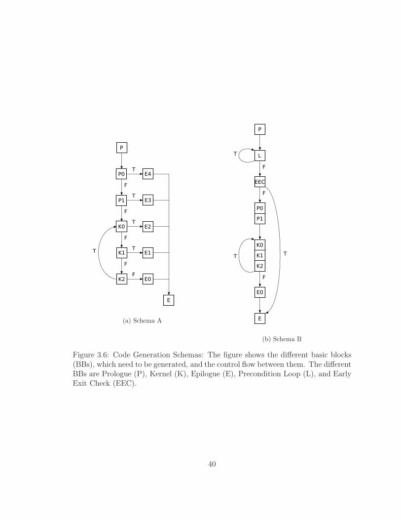
3.6 Code Generation

The code generation for software pipelined loop has a wide variety of schemas

it can use depending on the available architectural features. Architectures which

support predication and special branch instructions, like the Itanium architecture,

allow the generation of kernel-only code [49]. There is no need for the code generator

to create additional code for the prologue and the epilogue, which allows the gen-

eration of very compact code. Another feature, which may affect code generation,

is rotating registers. If rotating registers are present, the kernel does not need to

be unrolled for modulo variable expansion (MVE). This also allows more compact

code. If this feature is not present, then there are several ways the code generator

can create code. One important factor we have to consider, is that there may be

more than one kernel version, due to MVE. Furthermore, the number of iterations

might not be known during compile time, which means the loop can exit at any of

38

the prologues or kernels. Due to the different register assignments in the prologues

and kernels, a dedicated epilogue has to be crafted for every possible case, resulting

in larger code. Another way to circumvent this problem is to generate a copy of

the loop before the software pipelined loop. This loop copy has to run for a certain

amount of iterations, so that it is guaranteed that the SWP loop will always exit at

the last kernel. Thus, only one epilogue is needed. Even though we have duplicated

the loop, the code size may still be smaller, because we got rid of different epilogue

versions. Figure 3.6 shows the two different code generation schemas mentioned

above. The are other possible variations of these schemas which can be used to

generate code that performs better or reduces code size. A list of possible schemas

for code generation can be found here [48].

39

(a) Schema A

(b) Schema B

Figure 3.6: Code Generation Schemas: The figure shows the different basic blocks(BBs), which need to be generated, and the control flow between them. The differentBBs are Prologue (P), Kernel (K), Epilogue (E), Precondition Loop (L), and EarlyExit Check (EEC).

40

Chapter 4

IMPLEMENTATION

The software pipelining framework was implemented in the PathScale EKOPath

compiler for the SiCortex Multiprocessor architecture. This chapter will explain the

different modules which have been used or implemented to enable software pipelining

for simple core architectures. During this whole chapter the same example loop will

be used and the transformations of every module to it will be shown. The reduction

loop, already introduced in Section 1, will be used as an example. Figure 4.1 shows

the reduction loop C code and Figure 4.2 shows the various transformation of the

corresponding pseudo assembly code before software pipelining.

int i ;double sum = 0 . 0 ;

for ( i = 0 ; i < SIZE ; ++i ) {sum += a [ i ] ;

}

Figure 4.1: Reduction Loop (C-Code)

4.1 Overview of the Framework

The software pipelining framework in the PathScale EKOPath compiler (a

commercial x86 and MIPS compiler based on Open64) is part of a multi-level opti-

mization framework for loops. Starting at the outer level we have the general loop

optimization framework, which analyzes the different loops, one at a time, starting

41

loop :TN243 :− ldc1 GTN238 [ 1 ] (0 x0 )



(a) original assembly code

loop :TN267 :− ldc1 GTN277 [ 1 ] (0 x0 )

GTN271 :− add . d TN267 GTN271 [ 1 ]TN274 :− daddiu GTN277 [ 1 ] (0 x8 )TN268 :− ldc1 TN274 (0 x0 )



GTN241 :− add . d TN270 GTN241 [ 1 ]GTN277 :− daddiu TN276 (0 x8 )


(b) after recurrence breaking and loop unrolling

loop :TN267 :− ldc1 GTN277 [ 1 ] (0 x0 )






(c) after extended block optimization (EBO)

Figure 4.2: Reduction Loop (Pseudo Assembly Code)

42

at the innermost loop level. Even though we only optimize the innermost loop level,

it is also necessary to check the outer loop levels. This is necessary because we may

fully unroll an inner loop during loop optimization, which makes the innermost loop

level disappear. Loops are divided into two categories - DO-LOOPS and WHILE-

LOOPS. These two categories are further sub-divided, depending on the properties

of the loop we would like to optimize. One of the most important criteria is the

number of basic blocks (BBs). Most advanced loop optimization techniques, like

software pipelining, can only be performed on a single BB. It is possible to perform

software pipelining on WHILE-LOOPS, but it requires special hardware support.

Since the current implementation targets a processor which does not support spec-

ulation, software pipelining is not performed on WHILE-LOOPS. Multi-BB loops

are also not supported by the current software pipeliner and are therefore scheduled

with the Hyper-Block Scheduler (HBS).

If the loop optimization framework finds a suitable loop for software pipelin-

ing, further optimizations are performed before the loop is finally passed on to the

software pipelining framework. These include loop unrolling, recurrence breaking,

induction variable removal, load store elimination and extended block optimization

(EBO). After all these optimizations and transformations have been performed, the

software pipelining framework is invoked to do the scheduling, register allocation

and code generation of the loop.

The first step is the calculation of the data dependence graph (DDG), fol-

lowed by the calculation of the minimum initiation interval (MII). Then the modulo

scheduler uses this information to find a schedule. If successful, modulo variable

expansion (MVE) and then register allocation (RA) are performed. If register al-

location fails, the framework gives up and the loop is restored to its original form.

Otherwise, we continue with the final step - code generation (CG) (see Figure 4.3).

43

Figure 4.3: Software Pipelining Framework

4.2 Data Dependence Graph (DDG)

Data dependence graph calculation is an integral part of every compiler.

Since there is already a DDG framework, which can generate cyclic DDGs for the

Itanium software pipeliner, there was no need to reimplement it in the context of

this thesis. The current DDG framework can calculate non-cyclic DDGs for single-

and multiple-BBs. Cyclic DDGs, on the other hand, can only be generated for single

BBs. The DDG which is generated for software pipelining does not have anti- or

output-dependencies for registers, because they can be removed by register renaming

(see Section 3.2 and 3.4). Figure 4.4 shows the DDG for the reduction loop example

in Figure 4.2c.

4.3 Minimum Initiation Interval

After the DDG for the loop has been obtained, the resource- and recurrence-

minimum initiation intervals are calculated. The resource minimum initiation in-

terval (ResMII) is calculated by simply adding up the resource requirements of all

instructions in the loop. The example loop uses four different instructions - load

44

Figure 4.4: Data Dependence Graph for Reduction Loop Example

double word to floating-point register (ldc1), floating-point double word addition

(add.d), unsigned integer double word addition (daddiu) and branch if not equal

(bne). The resource requirements for the different instructions are displayed in Fig-

ures 4.5a to 4.5d. The total resource requirements for the whole loop are shown

in Figure 4.5e. To calculate ResMII, each resource is checked and the maximum

resource usage defines ResMII. Issue Slots requires twelve resources, but there are

two of this type available. Therefore the resource requirements for Issue Slot are six

(12/2). The Execution Unit also requires six resources (6/1). The Multiply/Divide

Unit does not have any requirements. The Floating-Point Unit requires four re-

sources (4/1). The resources Issue Slot and Execution Unit are the limiting factors

in this example, resulting in a ResMII of six.

The recurrence minimum initiation interval (RecMII) calculation in this com-

piler is based on Monica Lam’s method [53], by first finding all the elementary

circuits (also known as strongly connected components (SCC)) in the DDG using

Tarjan’s algorithm [64] and then solving the all-points longest path problem for each

SCC with Floyd’s algorithm [65]. Figure 4.6 shows all the elementary circuits of the

45

(a) Ressource Requirements for ldc1 (b) Resource Requirements for add.d

(c) Resource Requirements for daddiu (d) Resource Requirements for bne

(e) Resource Requirements for the Loop

Figure 4.5: Resource Requirements: Issue Slot (Is), Execution Unit (Ex), Multi-ply/Divide Unit (MD), Floating-Point Unit (FP)

DDG. The resulting individual recurrence initiation intervals are four (4/1), four

(4/1), four (4/1), four (4/1), and one (1/1). Thus, RecMII for this example loop is

four.

Figure 4.6: Recurrence MII

The combination of ResMII and RecMII yield a MII of six.

46

4.4 Modulo Scheduler

The modulo scheduler is the most important, and also the most compile time

consuming, part of the framework. In general, a modulo scheduler tries to place the

instructions of one loop iteration, one at a time, into free issue slots, considering the

dependence and resource constraints. Figure 4.7a shows one possible schedule for

the reduction loop example from Figure 4.2. The corresponding modulo reservation

table (MRT) is shown in Figure 4.7b. Since the processor is dual-issue capable, there

are two issue slots displayed in the MRT. Ex represents the Execution Unit, MD

the Multiply/Divide Unit and FP the Floating-Point Unit. The branch instruction

of this architecture cannot be dual-issued and can also only have one instruction

in the delay slot. Therefore, the branch instruction occupies both issue slots when

it is issued and one issue slot in the cycle after. The resulting kernel has 2 stages

and is shown in Figure 4.7c. The current modulo scheduler implementation is based

(a) ModuloSchedule

(b) Modulo Reservation Table (c) Kernel

Figure 4.7: Modulo Scheduler

on Huff’s Lifetime-Sensitive Modulo Scheduler [16]. Huff’s modulo scheduler idea

is based on his slack-scheduling framework. Each instruction may have a certain

freedom when it can be scheduled. His entire framework is built around the notion

of instruction scheduling freedom - or ”slack” for short. The slack of one instruction

is defined as the difference of its latest and earliest starting time.

47

First, two new instructions are introduced to the loop - start and stop. Start

and stop are two fake instructions, which are used in the following calculations

and during scheduling. They will be removed after the scheduler is finished. All

instructions of the loop depend on start and therefore start needs to be scheduled

in cycle 0. Stop, on the other hand, depends on all instructions of the loop. Stop is

scheduled like any other instruction of the loop.

The earliest (Estart) and latest (Lstart) time are calculated with the help of

the minimum distance relation.

Definition 4.4.1. MinDist(x,y) is the minimum number of cycles (possibly nega-

tive) by which x must precede y in any feasible schedule, or −∞ if there is no path

in the dependence graph from x to y [16].

MinDist is an all-pairs longest-paths problem, but can be converted to a all-

pairs shortest-paths problem, by negating the weight of each arc. Afterwards the

values on the first diagonal are set to zero. Figure 4.8 shows the pseudo code for

the MinDist calculation. The resulting MinDist matrix for the example loop can be

seen in Table 4.1.

If the first diagonal of the MinDist matrix is not set to zero yet, the given II

value can be verified. The values on the diagonal specify the schedule distance in

cycles of each operation to itself. Positive values in the diagonal indicate that the

calculated II is incorrect and too small. All values on the diagonal should be zero or

negative. After the verification, all the values on the first diagonal are set to zero.

Estart and Lstart can then be computed with the help of the MinDist relation.

The formulas for Estart and Lstart are defined as follows:

Definition 4.4.2. Estart(x) = MinDist(START, x) and

Lstart(x) = Lstart(STOP )−MinDist(x, STOP ), where x is any given operation

of the loop and START/STOP denote the two fake operations.

48

/∗ I n i t i a l i z e the minimum d i s t an c e matrix to −INFINITY ∗/

/∗ Set arc we igh t s ∗/for each ope ra t i on i o f the loop {

for each su c c e s s o r j o f ope ra t i on i {MinDist ( i , j ) =

max ( MinDist ( i , j ) , l a t ency ( i , j ) − omega ( i , j ) ∗ I I ) ;}

/∗ Every OP has a dependence to START and STOP with weight 0 ∗/MinDist (START, i ) = 0 ;MinDist ( i ,STOP) = 0 ;

}

/∗ Floyd−Warshal l Al l−Pairs Sho r t e s t Path Algorithm ∗/for each ope ra t i on k o f the loop {

for each ope ra t i on i o f the loop {for each ope ra t i on j o f the loop {

MinDist ( i , j ) =max ( MinDist ( i , j ) , MinDist ( i , k ) + MinDist (k , j ) ) ;

}}

}

for each ope ra t i on i o f the loop {MinDist ( i , i ) = 0 ;

}

Figure 4.8: MinDist Pseudo Code

The earliest and latest possible starting time is calculated for every instruc-

tion, as well as the slack, which is just the difference of the former two. Table 4.2

shows the Estart, the Lstart and the Slack for the example loop.

Furthermore, it is calculated which hardware resources are in high demand.

This information is later needed for the scheduling heuristic. Then the scheduler

begins to schedule one instruction at a time. A heuristic decides which instruction

needs to be scheduled next. This is done by assigning a priority to each instruction,

which depends on the current slack of the instruction and on the critical hardware

resource requirements. After an instruction has been chosen by the heuristic, we

49

Table 4.1: MinDist Table: This table shows the minimum distance relation in matrixform. The numbers in the first row and in the first column represent the OP numbersof the loop. OP 0 and OP 11 are the two fake operations START and STOP,respectively. The numbers inside the matrix show if there is a dependence betweentwo operations and what the minimum distance between these two operations hasto be. A −∞ indicated that there is no dependence between the two operations.

OP 0 1 2 3 4 5 6 7 8 9 10 11

0 0 0 3 0 3 0 3 0 3 0 1 31 −∞ 0 3 −∞ −∞ −∞ −∞ −∞ −∞ −∞ −∞ 32 −∞ −∞ 0 −∞ −∞ −∞ −∞ −∞ −∞ −∞ −∞ 03 −∞ −∞ −∞ 0 3 −∞ −∞ −∞ −∞ −∞ −∞ 34 −∞ −∞ −∞ −∞ 0 −∞ −∞ −∞ −∞ −∞ −∞ 05 −∞ −∞ −∞ −∞ −∞ 0 3 −∞ −∞ −∞ −∞ 36 −∞ −∞ −∞ −∞ −∞ −∞ 0 −∞ −∞ −∞ −∞ 07 −∞ −∞ −∞ −∞ −∞ −∞ −∞ 0 3 −∞ −∞ 38 −∞ −∞ −∞ −∞ −∞ −∞ −∞ −∞ 0 −∞ −∞ 09 −∞ -5 -2 -5 -2 -5 -2 -5 -2 0 1 110 −∞ −∞ −∞ −∞ −∞ −∞ −∞ −∞ −∞ −∞ 0 011 −∞ −∞ −∞ −∞ −∞ −∞ −∞ −∞ −∞ −∞ −∞ 0

need to check if there are free resources in the modulo reservation table, between the

latest and earliest starting times. The search direction, which decides if we want

to place an instruction later or earlier, is based on another heuristic, which tries

to minimize register lifetime. More details about the heuristic can be found in the

paper [16]. If the scheduler cannot find free resources, it is forced to choose a time

slot. This time slot may violate dependence constraints and/or resource constraints.

Instructions which have already been scheduled and violate any of the dependence

constraints will be unscheduled, including all its successors and predecessors. If there

are not enough free resources to schedule the selected instruction, other instructions

which use the same resources or relevant resources will be unscheduled until the

scheduler can place the new instruction. After an instruction has been placed,

the earliest and latest starting times and slack are recalculated, because the newly

50

Table 4.2: Slack: OP 0 and OP 11 are the two fake operations START and STOP,respectively.

OP Estart Lstart Slack

0 0 2 21 0 2 22 3 5 23 0 2 24 3 5 25 0 2 26 3 5 27 0 2 28 3 5 29 0 4 410 1 5 411 3 5 2

placed instruction may have affected the earliest and/or latest starting times of other

instructions. The formula for updating Estart/Lstart is given below:

Definition 4.4.3. Estart = max(Estart(x), t + MinDist(y, x)) and

Lstart = max(Lstart(x), t −MinDist(x, y)), where y is the currently placed OP

and t is the scheduled cycle.

This step is repeated until the scheduler is able to schedule all instructions.

This is not always possible for a given II. Every instruction has a budget. Every

time an instruction is scheduled, the budget is decreased. If the budget of one

instruction is depleted, the modulo scheduler gives up and tries another II. To

reduce compilation time, the search space for a schedule is first pruned by searching

for a valid schedule with exponential increasing steps for II. Then a binary search

is performed in this pruned search space.

51

4.5 Modulo Variable Expansion

The modulo scheduler scheduled the instructions on the premise that there

are no anti- or output-dependencies for registers. To guarantee this, a unique Tem-

porary Name (TN)1 set for every iteration needs to be provided. Register renaming

is performed according to [17, 53]. First, the lifetime of every TN is calculated.

The longest lifetime determines how often the kernel has to be unrolled. Then, the

kernel is unrolled and every loop iteration gets a new TN set assigned (see Figure

4.9).

4.6 Register Allocator

After modulo variable expansion, the lifetime of every TN is recalculated.

The register allocator, which is based on [47], is provided with the start cycle,

end cycle, ω value and α value of every TN. The start cycle defines when the TN

has been defined by an instruction. The end cycle is determined by instructions

which use the TN and the corresponding ω value. ω defines the iteration distance

as described in Section 3.1. α defines if a value is live-out of the loop. The α

value shows, as for ω, at which iteration the value has been produced. First, all

loop-invariant TNs are register allocated, thus reducing the available register set.

Then the loop-variant TNs are allocated. The lifetimes are sorted by start and end

cycle. Then an interference matrix of the lifetimes is calculated. Every lifetime is

initialized with the remaining free register set. Lifetimes are allocated by picking the

first free register in the remaining register set. Then the register is removed from

all interfering lifetimes’ register sets. This process is continued until all TNs are

register allocated (unless there are no more free registers). Registers are chosen by

the “First Fit” approach as described in [47], but with the extension that caller-save

registers are used first, and callee-save registers are used only if necessary.

1 TNs are the internal representation of the compiler for any type of operand orresult of an instruction

52

TN mapping :TN239 −> TN280 , TN280 ( loop i nva r i an t )TN241 −> TN295 , TN296TN267 −> TN285 , TN286TN268 −> TN283 , TN284TN269 −> TN293 , TN294TN270 −> TN297 , TN298TN271 −> TN281 , TN282TN272 −> TN287 , TN288TN273 −> TN289 , TN290TN277 −> TN291 , TN292

Kernel 1 :TN282 :− add . d TN286 [ 1 ] TN281 [ 1 ]TN283 :− ldc1 TN292 [ 1 ] (0 x8 )TN285 :− ldc1 TN292 [ 1 ] (0 x0 )TN288 :− add . d TN284 [ 1 ] TN287 [ 1 ]TN290 :− add . d TN294 [ 1 ] TN289 [ 1 ]TN291 :− daddiu TN292 [ 1 ] (0 x20 )TN293 :− ldc1 TN292 [ 1 ] (0 x10 )TN296 :− add . d TN298 [ 1 ] TN295 [ 1 ]

:− bne TN291 [ 0 ] TN280 [ 0 ]TN297 :− ldc1 TN292 [ 1 ] (0 x18 )

Kernel 2 :TN281 :− add . d TN285 [ 0 ] TN282 [ 0 ]TN284 :− ldc1 TN291 [ 0 ] (0 x8 )TN286 :− ldc1 TN291 [ 0 ] (0 x0 )TN287 :− add . d TN283 [ 0 ] TN288 [ 0 ]TN289 :− add . d TN293 [ 0 ] TN290 [ 0 ]TN292 :− daddiu TN291 [ 0 ] (0 x20 )TN294 :− ldc1 TN291 [ 0 ] (0 x10 )TN295 :− add . d TN297 [ 0 ] TN296 [ 0 ]

:− bne TN292 [ 0 ] TN280 [ 0 ]TN298 :− ldc1 TN291 [ 0 ] (0 x18 )

Figure 4.9: Modulo Variable Expansion of the Example Code

53

This register allocator is only applicable to software-pipelined kernels and is

independent of the code generator’s normal register allocators, which are the local

register allocator (LRA) and the global register allocator (GRA).

Minor changes in LRA and GRA are needed to support software pipelining.

In particular, LRA and GRA must preserve the register assignment made by the

software pipeliner. In the case of LRA, LRA is simply not run for the software-

pipelined basic blocks. For GRA, the problem is harder. In the past, a non-open-

sourced version of software pipelining used regions to delimit basic blocks which are

register-allocated by the software pipeliner. GRA would allocate all basic blocks

except those in the region. ”Glue copies” are inserted at region boundaries to rec-

oncile register assignment differences across the boundary. These copies are normal

register copies that have partial register assignment. It is up to GRA to make the

copy redundant by allocating the same register to both sides. Redundant copies are

removed afterwards by the extended block optimizer (EBO). If GRA cannot allocate

the same register to both sides, the glue copy becomes a real copy.

In the current implementation, instead of using regions, GRA is modified to

handle partial register allocation made by earlier phases such as software pipelining.

In a partial allocation, some but not all variables have assigned registers. When

GRA runs, it builds live-ranges for all global variables as usual. In the coloring

step, GRA detects those live-ranges that have assigned registers and prioritizes

them first, so that when they are colored, GRA can always color them with their

assigned register. In addition, for local variables (those spanning one basic block)

with assigned registers, GRA removes their registers from the allocation set for

that basic block, thus preserving the allocation to these local variables. With these

modifications, GRA can handle partial allocations with minimal changes to the GRA

algorithm.

54

4.7 Code Generator

The code generator performs the final step in the software pipelining frame-

work. There are several ways the final code can be generated. A list of several code

generation schemas can be found here [48]. The approach used in this framework

is based on the paper mentioned above, with one additional optimization for archi-

tectures with static branch prediction. Figure 4.10a shows the control flow graph

(CFG), which will be created for the example loop. Prologues, kernels and epilogues

(a) Control Flow Graph (b) BB Content

Figure 4.10: Code Generation Schema

are marked with P, K and E, respectively. Jump blocks are marked with JB. Arrows

show the control flow between the BBs. T or F on the arrows indicates if the branch

is taken (T) or if it is a fall-through (F). The small number next to the BB indicates

the actual order of the BBs in the assembly file. The example loop has a kernel with

two stages and the kernel needs to be unrolled two times for MVE. Furthermore,

one prologue stage and one epilogue stage are needed.

55

The first BB (P) contains copies for loop-invariant variables and falls through

to the BB (P0), which starts the first loop iteration. If the loop has just one iteration,

then we jump to P0’s designated epilogue BB (E2). Otherwise, we continue with

K0. The BBs K0 and K1 represent the unrolled kernel. Each BB uses a different

register set. The targeted architecture uses static branch prediction, which assumes

that every branch is taken. That is the reason why the branches between the kernel

BBs are forward jumps instead of fall-throughs. Every kernel BB follows a jump

block (except the last one). If the loop is finished, then the kernel BB K0 falls

through to its jump block, which only contains an unconditional branch to the

kernel’s designated epilogue BB. Every kernel BB needs its own epilogue, because

every kernel uses a different register set. Instead of the jump blocks, it is possible

to insert the epilogues themselves, but for cache performance reasons this thesis

introduces the jump block.

Figure 3.6b shows the content of the BBs in more detail. A and B represent

the two different stages of the kernel. The number indicates which register set is

used.

56

Chapter 5

EXPERIMENTS

To test the new software pipelining framework, we used two testbeds with

distinct requirements. One testbed is an extensive collection of simple test cases,

commercial and academic applications, and compiler validation suites, among oth-

ers. This testbed is used to test the correctness of the generated code. The other

testbed is composed of the NAS Parallel Benchmarks [66, 67, 68] and the SPEC

2006 benchmark suite [69], and is used to test the performance of the generated

code.

The first testbed is beyond the scope of this thesis. However, the current

software pipelining framework has already passed this testbed successfully. Results

for the second testbed are described in this chapter.

5.1 Testbed

The software pipelining framework was tested on a SiCortex Multiprocessor

system [8]. The system used for the experiments is an internal testing system and

not available on the market. The test system is very similar to the SC072-PDS

and consists of one System Service Processor (SSP) and four compute nodes. The

SSP is an AMD Athlon 3000+ processor with 1 GB of main memory. The compute

nodes are SiCortex Multiprocessors ICE9B V1.0 FPU V0.1 with 8 GB of main

memory each. Each SiCortex Multiprocessor has six cores and runs at 500 Mhz.

The main difference between the SC072-PDS and the test system is that the test

system only has four SiCortex Multiprocessor chips, instead of twelve. The operating

57

system running on the SSP is Red Hat Enterprise Linux. The compute nodes run a

modified version of Gentoo Linux for MIPS. Each processor has a peak performance

of 1 GFLOP - amounting to 6 GFLOPs for one chip. Newer versions of the chip

run at 700 MHz and provide 8.4 GFLOPs of peak performance [50].

The software pipelining framework was implemented in a development version

of the PathScale EKOPath compiler for the SiCortex Multiprocessor architecture.

The development version is a beta version of the upcoming PathScale EKOPath

compiler release version 3.3.

The NAS Parallel Benchmarks and the SPEC 2006 Benchmarks were chosen

to measure the performance impact. The NAS Parallel Benchmarks are a small

set of kernels, which are used to evaluate the performance of parallel computers.

The benchmarks are also relatively small, which makes them easier to analyze and

instrument. For the purpose of this thesis, we use the serial version of the NAS

Parallel benchmarks and run them on only one processor. By doing so, we can

eliminate any overhead and fluctuations due to cross-processor synchronizations.

The SPEC 2006 Benchmark Suite became a industry standard to evaluate

the performance of computer systems. The suite consists of several integer and

floating-point benchmarks of real world applications with real world testing data to

stress the cpu and the memory system. The suite is also used by compiler vendors

to evaluate and compare their compiler against other compiler vendors.

Table 5.1 lists and briefly describes the different benchmarks of the NAS

Parallel Benchmarks version 3.3. Table 5.2 and Table 5.3 explain briefly the several

integer and floating-point benchmarks of the SPEC 2006 benchmark suite.

5.2 Results

The NAS Parallel Benchmarks (serial version 3.3) were compiled with the

class A test size for the 32 and 64 bit ABI. The only flags passed to the compiler

were -O3 -ipa. Test results were obtained for all benchmarks expect the 32 bit

58

Table 5.1: NAS Parallel Benchmarks

Benchmark Description

BT BT is a solver of the 3-D compressible Navier-Stokesequations.

CG CG is a program that uses the conjugate gradient methodto find the smallest eigenvalue of a sparse matrix.

DC DC performs data cube operations on a large arithmeticdata set to test data movement across memory hierar-chies of grid machines.

EP EP is an Embarrassingly Parallel program that estab-lishes the reference point for the peak performance of thesystem.

FT FT is a 3-D Fast Fourier Transform (FFT) kernel.IS IS is integer sort, which tests integer computation speed

and communication performance.LU LU is another Computational Fluid Dynamics applica-

tion (BT and SP are also used for CFD applications)which uses symmetric Successive over-relaxation to findsolutions of the Navier-Stokes equations in 3-D.

MG MG calculates the solution of the 3-D scalar Poissonequation using a V-Cycle MultiGrid method. It is usedto test near and far data movements.

SP SP is similar to BT but it uses a Beam-Warming approx-imate factorization.

UA UA solves a heat transfer problem on an unstructuredmesh.

59

Table 5.2: SPEC 2006 Integer Benchmarks


400.perlbench A modified version of Perl v5.8.7. It consists of SpamAssassin, an email indexer and the SPEC’s specdiff tool.

401.bzip2 A modified version of bzip2 v1.0.3 which does most of itswork in memory rather than doing it in I/O.

403.gcc A simplified version of GNU GCC 3.2 that generates codefor Opteron architectures.

429.mcf An implementation of the network simplex algorithm. Itis used for vehicle scheduling.

445.gobmk A simulation of the game of Go.456.hmmer A bio informatics application. It is a protein sequencer

which uses profile hidden Markov models.458.sjeng A chess simulator.462.libquantum The simulation of the Shor’s polynomial-time factoriza-

tion algorithm running on a quantum computer.464.h264ref A model implementation of a video encoder

(H.264/AVC) which encodes a videostream with 2parameter sets.

471.omnetpp A modeling of a large ethernet campus network using theOMNet++ discrete event simulator.

473.astar A 2D map path finder library. It includes the well-knownA* algorithm.

483.xalancbmk A modified clone for an XML to many format converter(i.e. Xalan-C++).

60

Table 5.3: SPEC 2006 Floating-Point Benchmarks


410.bwaves Computes 3D transonic transient laminar viscous flow.416.gamess A quantum chemical computations simulator.433.milc Program used to generate gauge fields for lattice gauge

theory programs.434.zeusmp A simulator of astrophysical phenomena using computa-

tional fluid dynamics principles.435.gromacs A molecular dynamics simulator for the protein

Lysozyme in a solution.436.cactusADM A solver for the Einstein evolution equations.437.leslie3d Computational Fluid Dynamics program for large Eddy

simulations444.namd Simulator for biomolecular systems.447.dealII A library written in C++ for adaptive finite elements

and error estimation.450.soplex A solver that uses the simplex algorithm and sparse linear

algebra.453.povray A simplified version of a famous ray tracer.454.calculix An application for finite element code used for linear and

nonlinear 3D structural applications.459.GemsFDTD A solver for 3D Maxwell equations using the FDTD

method.465.tonto A quantum chemistry package.470.lbm Simulates incompressible fluids using the Lattice Boltz-

mann Method in 3D.481.wrf A weather simulator with variable time and space param-

eters.482.sphinx3 The Carnegie Mellon University’s speech recognition sys-

tem.

61

Table 5.4: NAS Parallel Benchmarks Results (32 bit)

w/o SWP w/ SWPBenchmark Time (s) Time (s) Speedup

BT 813.27 812.79 1.00CG 50.45 43.75 1.15DC n/a n/a n/aEP 210.83 207.48 1.02FT 103.26 110.53 0.93IS 14.78 14.73 1.00LU 919.88 918.91 1.00MG 37.87 40.23 0.94SP 918.87 898.31 1.02UA 490.49 490.70 1.00

version of DC. The verification for this benchmark failed. This was not a problem

of SWP, but of the used beta compiler in general. The tests were run twice - once

with software pipelining disabled for the baseline and once with software pipelining

enabled. Table 5.4 shows the results for the 32 bit version of the benchmark. The

results for the 64 bit version are shown in Table 5.5. The speedup for both ABI

testruns is displayed in Figure 5.1.

The SPEC 2006 Benchmarks Suite was also compiled for the 32 and 64 bit

ABI. The only flags passed to the compiler were -O3 -ipa. Test results were obtained

for all benchmarks expect for 483.xalancbmk and 416.gamess. 483.xalancbmk is not

SWP related, and 416.gamess failed due to a wrong data dependence graph. The

tests were run twice - once with software pipelining disabled for the baseline and

once with software pipelining enabled. Table 5.6 shows the results for the 32 bit

version of the benchmark. The results for the 64 bit version are shown in Table 5.7.

The speedup for both ABI testruns is displayed in Figure 5.2.

Experimental results show that even though the framework has a maximum

improvement of 15% for the 32bit CG benchmark, it also has some performance

62

Table 5.5: NAS Parallel Benchmark Results (64 bit)

w/o SWP w/ SWPBenchmark Time (s) Time (s) Speedup

BT 824.37 831.29 0.99CG 44.24 43.36 1.02DC 32674.21 31605.34 1.03EP 214.59 209.41 1.02FT 110.04 109.46 1.01IS 14.72 14.71 1.00LU 911.44 914.25 1.00MG 38.93 41.42 0.94SP 912.90 886.63 1.03UA 490.20 487.40 1.01

Figure 5.1: NAS Parallel Benchmark Speedup

63

Table 5.6: SPEC 2006 Results(32 bit)

w/o SWP w/ SWPBenchmark Time (s) SPEC Ratio Time (s) SPEC Ratio Speedup

400.perlbench 9219.20 1.06 9326.90 1.05 0.99401.bzip2 9237.30 1.04 9202.90 1.05 1.00403.gcc 5944.70 1.35 5944.90 1.35 1.00429.mcf 5131.70 1.78 5086.10 1.79 1.01445.gobmk 7272.10 1.44 7097.70 1.48 1.02456.hmmer 9811.60 0.95 9940.60 0.94 0.99458.sjeng 8349.50 1.45 8309.30 1.46 1.00462.libquantum 7441.80 2.78 7422.30 2.79 1.00464.h264ref 10494.50 2.11 10632.10 2.08 0.99471.omnetpp 4066.50 1.54 4099.40 1.52 0.99473.astar 4659.60 1.51 4691.80 1.50 0.99483.xalancbmk n/a n/a n/a n/a n/a410.bwaves 8072.50 1.68 7981.30 1.70 1.01416.gamess n/a n/a n/a n/a n/a433.milc 4436.70 2.07 4428.80 2.07 1.00434.zeusmp 7598.40 1.20 7250.90 1.26 1.05435.gromacs 6121.40 1.17 6086.20 1.17 1.01436.cactusADM 7096.90 1.68 7043.60 1.70 1.01437.leslie3d 9639.00 0.98 9557.40 0.98 1.01444.namd 5706.50 1.41 5706.00 1.41 1.00447.dealII 6937.10 1.65 6970.20 1.64 1.00450.soplex 5504.80 1.52 5501.90 1.52 1.00453.povray 3646.60 1.46 3677.00 1.45 0.99454.calculix 6301.00 1.31 6348.90 1.30 0.99459.GemsFDTD 7795.60 1.36 8043.40 1.32 0.97465.tonto 9908.60 0.99 10084.60 0.98 0.98470.lbm 7843.70 1.75 7874.70 1.74 1.00481.wrf 10461.90 1.07 10552.70 1.06 0.99482.sphinx3 12889.90 1.51 12322.50 1.58 1.05Total 201589.10 201184.10 1.00

64

Table 5.7: SPEC 2006 Results (64 bit)

w/o SWP w/ SWPBenchmark Time (s) SPEC Ratio Time (s) SPEC Ratio Speedup

400.perlbench 9703.10 1.01 9978.80 0.98 0.97401.bzip2 10919.00 0.88 10943.40 0.88 1.00403.gcc 8046.00 1.00 8046.00 1.00 1.00429.mcf 6264.90 1.46 6211.80 1.47 1.01445.gobmk 7469.70 1.40 7693.60 1.36 0.97456.hmmer 9694.40 0.96 9811.20 0.95 0.99458.sjeng 8375.40 1.44 8544.00 1.42 0.98462.libquantum 7408.50 2.80 7465.10 2.78 0.99464.h264ref 13059.00 1.69 13626.00 1.62 0.96471.omnetpp 4471.90 1.40 4471.90 1.40 1.00473.astar 4737.20 1.48 4755.30 1.48 1.00483.xalancbmk n/a n/a n/a n/a n/a410.bwaves 8189.20 1.66 8090.60 1.68 1.01416.gamess n/a n/a n/a n/a n/a433.milc 4731.60 1.94 4689.80 1.96 1.01434.zeusmp 7683.10 1.18 7358.80 1.24 1.04435.gromacs 6264.70 1.14 6109.80 1.17 1.03436.cactusADM 6996.50 1.71 7034.40 1.70 0.99437.leslie3d 9785.30 0.96 9702.70 0.97 1.01444.namd 5734.10 1.40 5732.40 1.40 1.00447.dealII 8819.00 1.30 8711.40 1.31 1.01450.soplex 5673.60 1.47 5663.40 1.47 1.00453.povray 3968.70 1.34 4064.80 1.31 0.98454.calculix 6534.10 1.26 6382.50 1.29 1.02459.GemsFDTD 7936.80 1.34 8110.20 1.31 0.98465.tonto 10085.50 0.98 10550.50 0.93 0.96470.lbm 8260.30 1.66 8270.40 1.66 1.00481.wrf 10538.60 1.06 10697.00 1.04 0.99482.sphinx3 13343.90 1.46 12870.00 1.51 1.04Total 214694.10 215585.80 1.00

65

Figure 5.2: SPEC 2006 Speedup

degradation for other benchmarks. However, this degradation is not significant.

In general, the improvement from SWP depends on how much time each program

spends in loops, and what percentage of those loops can be software-pipelined.

Even among software-pipelined loops, small loops tend to exhibit larger percentage

improvement than large loops. Loops with a small number of iterations are not

screened out during run-time and therefore exhibit the overhead of the prologue and

epilogue. There are three main reasons why the results for the other benchmarks

are not better.

First, some of the main loops in these applications have calls to mathematical

operations, such as logarithms, exponentiation, etc, which are not inlined by the

Inter-Procedural Optimizer (IPO). This results in loops which have multiple basic

blocks for which the software pipeliner has no support. Normally, such functions

are intrinsics or macros in different architectures and libraries. In these cases, the

actual operation code is replaced by a short sequence of ISA instructions or with the

body of the operation itself (in the case of macros or inline functions respectively).

66

Second, some of the kernels in these applications have a very high register

usage which in turn increases register pressure. Since register spilling has not been

implemented for the software pipeliner, this limits the number of loops which can

be successfully software-pipelined. Hence, many optimizing opportunities are lost

due to the high register pressure being prevalent in the bigger kernels.

Third, the target architecture supports only one outstanding L1 cache miss.

All other following loads or stores must hit in L1 cache, otherwise the processor

will stall until the data of the first cache miss has been transfered to L1 cache. The

current target description does not model this behavior correctly, resulting in a non-

optimal schedule with unexpected stalls. Furthermore, prefetch instructions, which

should prevent or reduce L1 cache misses, are ignored by the target architecture if

there is already an outstanding L1 cache miss. Due to this, wrong latencies and

resource requirements are passed on to the software pipeliner, preventing it from

generating a better schedule.

Even with these limitations, the current implementation still delivers some

marginal performance improvement without degrading the overall performance pic-

ture. The maximum performance gain was seen to be 15 percent. On the other

hand, the maximum performance degradation was seen to be 7 percent. The soft-

ware pipeliner has reached production-quality and will be released by SiCortex this

April.

67

Chapter 6

RELATED WORK

There are several scheduling techniques under the umbrella of software pipelin-

ing. One of the best known techniques, and the most researched one, is modulo

scheduling. Optimal methods [70, 71, 57] have been researched and proposed, but

their high computational complexity due to NP-completeness prevents their use in

mainstream compilers. Nevertheless, they are an important instrument to validate

heuristic based modulo schedulers. Well known heuristic methods are Iterative Mod-

ulo Scheduling (IMS) [54, 55], Slack Modulo Scheduling (Slack) [16], Swing Modulo

Scheduling (SMS) [62], Hypernode Reduction Modulo Scheduling (HRMS) [61], and

others [72, 57, 73, 17, 53]. A comparison of several heuristic based modulo scheduling

techniques can be found here [74].

Iterative Modulo Scheduling (IMS) schedules instructions iteratively in order

given by the priority function which considers the height of the instruction in the

DDG. If an instruction can’t be placed in the partial schedule, the algorithm back-

tracks, unschedules already placed instructions and tries a different placement of

the instructions. This approach does not try to shorten lifetimes and may produce

schedules with higher register pressure than other lifetime-sensitive methods.

Slack Modulo Scheduling (Slack) schedules operations also based on a priority

function. The priority function considers the slack of an instruction and if the

instruction is using a critical hardware resource. The slack is simply the difference

of the earliest and latest starting times of a given instruction, which does change

68

during the scheduling process. Furthermore, it uses additional heuristics and a bi-

directional scheduling approach to shorten register-lifetime. If an instruction cannot

be placed in the partial schedule, then the conflicting instructions and its successors

and predecessors are removed from the schedule.

Swing Modulo scheduling (SMS) schedules a sorted list of instructions with-

out any backtracking, making this method less computationally expensive. The

instructions are sorted depending on the recurrence circuit they belong to and the

RecMII which is associated with it. Additional heuristics are applied to produce a

schedule with low register pressure.

Hypernode Reduction Modulo Scheduling (HRMS) uses a preordering phase

which sorts the instructions before scheduling. Elementary circuits are converted

during this process to hypernodes, starting with the circuit with the largest RecMII.

Nodes which are converted to hypernodes are added to the scheduling list. After

the preordering phase, the instructions are scheduled without backtracking.

The original MIPSpro compiler’s software pipeliner [57] employs modulo

scheduling and performs a binary search to reduce compilation time. The modulo

scheduler uses a branch-and-bound approach with several different sorting heuris-

tics for the priority list. The framework also uses modulo variable expansion (MVE)

and the register allocator supports register spilling for software pipelined kernels.

Furthermore, it performs memory bank optimization, which is specific to the MIPS

R8000 chip. Reservoir Labs licensed the MIPSpro compiler from SGI and provides

it as a closed-source compiler under the name Blackbird for the embedded market

[75]. This compiler contains the original software pipeliner for MIPS and is used by

Tilera for their MIPS-based chips [76].

All the methods mentioned above were designed for single core processors.

The two following modulo scheduling methods try to address this issue. Unfortu-

nately they still require certain hardware support, but they are a step toward a

69

software pipelining framework for many-core processors.

One of these techniques is Decoupled Software Pipelining (DSWP) [14]. De-

coupled Software Pipelining distributes the instructions of one loop iteration across

several cores and every core participates in all loop iterations, but it executes just a

certain part of the instructions. Another technique is Multi-Threaded Single Dimen-

sion Software Pipelining (MT-SSP) [15]. Multi-Threaded Single Dimension Software

Pipelining increases instruction level parallelism by modulo scheduling loop nests.

Furthermore, it distributes the iterations of the loop across the cores, instead of the

instructions as DSWP does. Each core executes a whole loop iteration, but may not

participate in all loop iterations.

70

Chapter 7

CONCLUSION AND FUTURE WORK

We have laid out the foundation of the software pipelining framework and

run it through our test harness to provide a robust implementation. We hope other

target architectures of the Open64 compiler will benefit from having the software

pipelining feature and we welcome any contributions from the Open64 community

to further enhance our open-sourced SWP framework.

An important area of improvement is to increase the percentage of loops

that can be software-pipelined, since many important loops could not be software-

pipelined because we were running out of registers. We hope to achieve this by

adding register spilling to the software pipelining framework.

Another important problem we need to address is the correct scheduling of

cache misses. Currently, the Open64 compiler assumes that every load is a hit in

L1 cache. We need to identify before the software pipelining framework which loads

are likely to miss and adjust their load latency and resource requirements. In this

way, not only the modulo scheduler, but also the normal list scheduler can take

advantage of this information to generate a better schedule. Only minor changes to

the software pipelining framework will be necessary in this case.

Further steps include the generation of a preconditioning loop to filter out

loops with a small number of iterations, in order to reduce the overhead of SWP for

these loops. This also enables new code generation schemas, which may reduce the

code size of the generated SWP schedule.

71

We also plan to implement other modulo scheduling techniques and verify

the results against an integer linear programming based scheduler, as it has been

done before for the MIPSpro compiler [57].

72

BIBLIOGRAPHY

[1] MIPS Technologies, Inc., 1225 Charleston Road, Mountain View, CA 94043-1353. MIPS64TM5KTMProcessor Core Family Software Users Manual, May2002.

[2] Han Q. Le, W. J. Starke, J. S. Fields, Francis P. O’Connell, D. Q. Nguyen,B. J. Ronchetti, Wolfram M. Sauer, Eric M. Schwarz, and Mike T. Vaden.IBM POWER6 microarchitecture. IBM Journal of Research and Development,51(6):639–662, 2007.

[3] William A. Wulf and Sally A. McKee. Hitting the Memory Wall: Implicationsof the Obvious. SIGARCH Comput. Archit. News, 23(1):20–24, 1995.

[4] John L. Hennessy and David A. Patterson. Computer Organization and De-sign: The Hardware/Software Interface. Morgan Kaufmann Publishers Inc.,San Francisco, CA, USA, 3rd edition, 2007.

[5] Ashlee Vance. IBM’s eight-core Power7 chip to clock in at 4.0GHz.http://www.theregister.co.uk/2008/07/11/ibm_power7_ncsa/, July2008.

[6] Roland Piquepaille. A thousand processors on one chip.http://blogs.zdnet.com/emergingtech/index.php?p=207, April 2006.

[7] Juan del Cuvillo, Weirong Zhu, Ziang Hu, and Guang R. Gao. TiNy Threads:a Thread Virtual Machine for the Cyclops-64 Cellular Architecture. In FifthWorkshop on Massively Parallel Processing (WMPP), April 2005.

[8] M. Reilly, L. C. Stewart, J. Leonard, and D. Gingold. SiCortex TechnicalSummary. 2006.

[9] Larry Seiler, Doug Carmean, Eric Sprangle, Tom Forsyth, Michael Abrash,Pradeep Dubey, Stephen Junkins, Adam Lake, Jeremy Sugerman, RobertCavin, Roger Espasa, Ed Grochowski, Toni Juan, and Pat Hanrahan. Larrabee:a many-core x86 architecture for visual computing. In SIGGRAPH ’08: ACMSIGGRAPH 2008 papers, pages 1–15, New York, NY, USA, 2008. ACM.

73

http://www.theregister.co.uk/2008/07/11/ibm_power7_ncsa/

http://blogs.zdnet.com/emergingtech/index.php?p=207

[10] Jaejin Lee, David A. Padua, and Samuel P. Midkiff. Basic compiler algorithmsfor parallel programs. SIGPLAN Not., 34(8):1–12, 1999.

[11] John L. Hennessy, David A. Patterson, and Andrea C. Arpaci-Dusseau. Com-puter Architecture: A Quantitative Approach. Morgan Kaufmann, 4th edition,2007.

[12] Leonardo Dagum and Ramesh Menon. OpenMP: an industry standard API forshared-memory programming. IEEE Computational Science & Engineering,5(1):46–55, 1998.

[13] Marc Snir, Steve W. Otto, David W. Walker, Jack J. Dongarra, and StevenHuss-Lederman. MPI: The complete reference. MIT Press, Cambridge, MA,USA, 1995.

[14] Guilherme Ottoni, Ram Rangan, Adam Stoler, and David I. August. Auto-matic Thread Extraction with Decoupled Software Pipelining. In MICRO 38:Proceedings of the 38th annual IEEE/ACM International Symposium on Mi-croarchitecture, pages 105–118, Washington, DC, USA, 2005. IEEE ComputerSociety.

[15] Alban Douillet and Guang R. Gao. Software-Pipelining on Multi-Core Archi-tectures. In Proceedings of the 16th International Conference on Parallel Ar-chitecture and Compilation Techniques, pages 39–48, Washington, DC, USA,2007. IEEE Computer Society.

[16] Richard A. Huff. Lifetime-Sensitive Modulo Scheduling. In PLDI ’93: Pro-ceedings of the ACM SIGPLAN 1993 Conference on Programming LanguageDesign and Implementation, pages 258–267, New York, NY, USA, 1993. ACM.

[17] Monica S. Lam. Software Pipelining: An Effective Scheduling Technique forVLIW Machines. In PLDI ’88: Proceedings of the ACM SIGPLAN 1988 Con-ference on Programming Language Design and Implementation, pages 318–328,New York, NY, USA, 1988. ACM.

[18] University of Tsukuba - High Performance ComputingSystem (HPCS) Laboratory. Omni OpenMP Compiler.http://www.hpcs.cs.tsukuba.ac.jp/omni-openmp.

[19] The SUIF Group. SUIF Compiler System. http://suif.stanford.edu.

[20] GCC Team. GCC, the GNU Compiler Collection. http://gcc.gnu.org.

74

http://www.hpcs.cs.tsukuba.ac.jp/omni-openmp

http://suif.stanford.edu

http://gcc.gnu.org

[21] University of Delaware - Computer Architecture and Parallel Sys-tems Laboratory (CAPSL). Open64 - The Open Research Compiler.http://www.open64.net.

[22] LLVM Developer. Low Level Virtual Machine (LLVM). http://llvm.org.

[23] NVIDIA Corporation. NVIDIA Compute Unified Device Architecture (CUDA).http://www.nvidia.com/cuda.

[24] NVIDIA Corporation. NVIDIA CUDA Compute Unified Device ArchitectureProgramming Guide, 2nd edition, June 2008.

[25] PathScale, LLC. http://www.pathscale.com.

[26] HP. http://www.hp.com.

[27] SimpLight Nanoelectronics, Ltd. http://www.simplnano.com.

[28] Qualcomm Inc. http://www.qualcomm.com/.

[29] Vinodha Ramasamy, Robert Hundt, Dehao Chen, and Wenguang Chen.Feedback-Directed Optimizations with Estimated Edge Profiles from HardwareEvent Sampling. 1st Open64 Workshop at CGO, April 2008.

[30] Hucheng Zhou, Xing Zhou, Tianwei Sheng, Dehao Chen, Jianian Yan, Shin-ming Liu, Wenguang Chen, and Weimin Zheng. A Practical Stride PrefetchingImplementation in Global Optimizer. 1st Open64 Workshop at CGO, April2008.

[31] Gautam Chakrabarti and Fred Chow. Structure Layout Optimizations in theOpen64 Compiler: Design, Implementation and Measurements. 1st Open64Workshop at CGO, April 2008.

[32] Subrato K. De, Anshuman Dasgupta, Sundeep Kushwaha, Tony Linthicum,Susan Brownhill, Sergei Larin, and Taylor Simpson. Development of an EfficientDSP Compiler Based on Open64. 1st Open64 Workshop at CGO, April 2008.

[33] Cody Addison, James LaGrone, Lei Huang, and Barbara Chapman. OpenMP3.0 Tasking Implementation in OpenUH. 2nd Open64 Workshop at CGO,March 2009.

[34] Silicon Graphics Inc. MIPSpro Compiler.http://www.sgi.com/products/software/irix/tools/mipspro.html.

[35] ORC - Open Research Compiler for Itanium Processor Family.http://ipf-orc.sourceforge.net.

75

http://www.open64.net

http://llvm.org

http://www.nvidia.com/cuda

http://www.pathscale.com

http://www.hp.com

http://www.simplnano.com

http://www.qualcomm.com/

http://www.sgi.com/products/software/irix/tools/mipspro.html

http://ipf-orc.sourceforge.net

[36] Richard M. Stallman and the GCC Developer Community. GNU CompilerCollection Internals. Free Software Foundation, Inc., 2008.

[37] Silicon Graphics, Inc. WHIRL Intermediate Language Specification, 2000.

[38] Keqiao Yang, Zhemin Yang, Zhiwei Cao, Zeng Huang, Di Wang, Min Yang,and Binyu Zang. Opencj: A research Java static compiler based on Open64.2nd Open64 Workshop at CGO, March 2009.

[39] Ron Cytron, Jeanne Ferrante, Barry K. Rosen, Mark N. Wegman, and Frank K.Zadeck. An efficient method of computing static single assignment form. InProceedings of the 16th ACM SIGPLAN-SIGACT symposium on Principles ofprogramming languages (POPL ’89), pages 25–35, New York, NY, USA, 1989.ACM.

[40] Ron Cytron, Jeanne Ferrante, Barry K. Rosen, Mark N. Wegman, and Frank K.Zadeck. Efficiently computing static single assignment form and the controldependence graph. ACM Transactions on Programming Languages and Systems(TOPLAS), 13(4):451–490, 1991.

[41] Fred Chow, Sun Chan, Shin-Ming Liu, Raymond Lo, and Mark Streich. Effec-tive Representation of Aliases and Indirect Memory Operations in SSA Form.LECTURE NOTES IN COMPUTER SCIENCE, pages 253–267, 1996.

[42] Fred Chow, Sun Chan, Robert Kennedy, Shin-Ming Liu, Raymond Lo, andPeng Tu. A new algorithm for partial redundancy elimination based on SSAform. In Proceedings of the ACM SIGPLAN 1997 conference on Programminglanguage design and implementation, pages 273–286. ACM New York, NY,USA, 1997.

[43] Shin-Ming Liu, Raymond Lo, and Fed Chow. Loop induction variable canoni-calization in parallelizing compilers. In Parallel Architectures and CompilationTechniques, 1996., Proceedings of the 1996 Conference on, pages 228–237, 1996.

[44] Mark N. Wegman and Frank K. Zadeck. Constant propagation with condi-tional branches. ACM Transactions on Programming Languages and Systems(TOPLAS), 13(2):181–210, Apr 1991.

[45] Intel Corporation. IntelR© Itanium R© Architecture Software Developers Manual,2006.

[46] Y. Choi, A. Knies, L. Gerke, and T. F. Ngai. The Impact of If-Conversionand Branch Prediction on Program Execution on the IntelR© ItaniumR© Proces-sor. In International Symposium on Microarchitecture: Proceedings of the 34

76

th annual ACM/IEEE international symposium on Microarchitecture: Austin,Texas, volume 1, pages 182–191, 2001.

[47] Bob R. Rau, Minsuk Lee, Parthasarathy P. Tirumalai, and Michael S.Schlansker. Register Allocation for Software Pipelined Loops. In Proceedingsof the ACM SIGPLAN 1992 conference on Programming language design andimplementation, pages 283–299. ACM New York, NY, USA, 1992.

[48] Bob R. Rau, Michael S. Schlansker, and Parthasarathy P. Tirumalai. CodeGeneration Schema For Modulo Scheduled Loops. In Microarchitecture, 1992.MICRO 25., Proceedings of the 25th Annual International Symposium on, pages158–169, 1992.

[49] Intel. Intel R©Itanium R©Architecture Software Developers Manual - Volume 1:Application Architecture, 2nd edition, January 2006.

[50] SiCortex, Inc., Three Clock Tower Place, 01754 Maynard, Massachusetts.SC072-PDS.

[51] T. C. Hu. Parallel Sequencing and Assembly Line Problems. Operations Re-search, 9(6):841–848, 1961.

[52] S.A. Mahlke, D.C. Lin, W.Y. Chen, R.E. Hank, and R.A. Bringmann. EffectiveCompiler Support for Predicated Execution Using the Hyperblock. In Proceed-ings of the 25th annual international symposium on Microarchitecture, pages45–54. IEEE Computer Society Press Los Alamitos, CA, USA, 1992.

[53] Monica S. Lam. A Systolic Array Optimizing Compiler. Kluwer Academic Pub,1989.

[54] Bob R. Rau. Iterative Modulo Scheduling: An Algorithm for Software Pipelin-ing Loops. In MICRO 27: Proceedings of the 27th Annual International Sym-posium on Microarchitecture, pages 63–74, New York, NY, USA, 1994. ACM.

[55] Bob R. Rau. Iterative Modulo Scheduling. Technical report, Hewlett Packard,November 1995.

[56] Roy F. Touzeau. A Fortran Compiler for the FPS-164 Scientific Computer.In SIGPLAN Symposium on Compiler Construction, volume 19, pages 48–57.ACM, June 1984.

[57] John Ruttenberg, Guang R. Gao, Arthur Stoutchinin, and W. D. Lichtenstein.Software Pipelining Showdown: Optimal vs. Heuristic Methods in a Production

77

Compiler. In Proceedings of the ACM SIGPLAN 1996 conference on Program-ming language design and implementation, pages 1–11. ACM New York, NY,USA, 1996.

[58] William M. Johnson. Superscalar Microprocessors Design. Prentice Hall PTR,December 1990.

[59] Robert M. Tomasulo. An Efficient Algorithm for Exploiting Multiple Arith-metic Units. IBM Journal of Research and Development, 11(1):25–33, 1967.

[60] Randy Allen and Ken Kennedy. Optimizing Compilers for Modern Architec-tures. Morgan Kaufmann, 2002.

[61] Josep Llosa, Mateo Valero, Eduard Ayguade, and Antonio Gonzalez. Hypern-ode Reduction Modulo Scheduling. In MICRO 28: Proceedings of the 28th An-nual International Symposium on Microarchitecture, pages 350–360, Los Alami-tos, CA, USA, 1995. IEEE Computer Society Press.

[62] Josep Llosa, Antonio Gonzalez, Eduard Ayguade, and Mateo Valero. SwingModulo Scheduling: A Lifetime-Sensitive Approach. In PACT, volume 96,pages 20–23.

[63] Javier Zalamea, Josep Llosa, Eduard Ayguade, and Mateo Valero. Improvedspill code generation for software pipelined loops. SIGPLAN Not., 35(5):134–144, 2000.

[64] Robert E. Tarjan. Depth-First Search and Linear Graph Algorithms. SIAMJournal on Computing, 1:146–160, 1972.

[65] Robert W. Floyd. Algorithm 97: Shortest Path. Communications of the ACM,5(6), 1962.

[66] D. H. Bailey, E. Barszcz, J. T. Barton, D. S. Browning, R. L. Carter, L. Dagum,R. A. Fatoohi, P. O. Frederickson, T. A. Lasinski, R. S. Schreiber, et al. TheNAS parallel benchmarks. International Journal of High Performance Com-puting Applications, 5(3):63, 1991.

[67] M.A. Frumkin and L. Shabanov. Arithmetic Data Cube as a Data IntensiveBenchmark. National Aeronautics and Space Administration, 2003.

[68] H. Feng, R.F. Van der Wijngaart, R. Biswas, and C. Mavriplis. UnstructuredAdaptive (UA) NAS Parallel Benchmark, Version 1.0. NASA Technical ReportNAS-04-006, 2004.

78

[69] J. L. Henning. SPEC CPU2006 benchmark descriptions. ACM SIGARCHComputer Architecture News, 34(4):1–17, 2006.

[70] Eric R. Altman and Guang R. Gao. Optimal Modulo Scheduling ThroughEnumeration. International Journal of Parallel Programming, 26(3):313–344,1998.

[71] A. E. Eichenberger, E. S. Davidson, and S. G. Abraham. Optimum ModuloSchedules for Minimum Register Requirements. In Proceedings of the 9th in-ternational conference on Supercomputing, pages 31–40. ACM New York, NY,USA, 1995.

[72] Paul Feautrier. Fine-Grain Scheduling under Resource Constraints. LECTURENOTES IN COMPUTER SCIENCE, pages 1–1, 1995.

[73] Amod K. Dani, V. Janaki Ramanan, and Ramaswamy Govindarajan. Register-Sensitive Software Pipelining. In Procs. of the Merged 12th International Par-allel Processing and 9th International Symposium on Parallel and DistributedSystems, April 1998.

[74] Josep M. Codina, Josep Llosa, and Antonio Gonzalez. A Comparative Studyof Modulo Scheduling Techniques. In ICS ’02: Proceedings of the 16th Inter-national Conference on Supercomputing, pages 97–106, New York, NY, USA,2002. ACM.

[75] Reservoir Labs Inc. Blackbird - HPEC Compiler.http://www.reservoir.com/blackbird.php.

[76] Wikipedia. Open64. http://en.wikipedia.org/wiki/Open64.

79

http://www.reservoir.com/blackbird.php

http://en.wikipedia.org/wiki/Open64

TOWARD A SOFTWARE PIPELINING FRAMEWORK FOR MANY-CORE CHIPS by Juergen Ributzka

Documents

Transcript of TOWARD A SOFTWARE PIPELINING FRAMEWORK FOR MANY-CORE CHIPS by Juergen Ributzka